$O(1)$ benchmarking of precise rotation in a spin-squeezed Bose-Einstein condensate

Abstract

Benchmarking a high-precision quantum operation is a big challenge for many quantum systems in the presence of various noises as well as control errors. Here we propose an $O(1)$ benchmarking of a dynamically corrected rotation by taking the quantum advantage of a squeezed spin state in a spin-1 Bose-Einstein condensate. Our analytical and numerical results show that tiny rotation infidelity, defined by $1-F$ with $F$ the rotation fidelity, can be calibrated in the order of $1/N^{2}$ by only several measurements of the rotation error for $N$ atoms in an optimally squeezed spin state. Such an $O(1)$ benchmarking is possible not only in a spin-1 BEC but also in other many-spin or many-qubit systems if a squeezed or entangled state is available.

I Introduction

High-precision quantum operations are among the most important building blocks for practical quantum computing and quantum information processing Nielsen and Chuang (2002), as well as for entanglement-enhanced quantum sensing beyond the standard quantum limit Giovannetti et al. (2004); Xu et al. (2019); Ma et al. (2011); Bao et al. (2020); Duan et al. (2000); Pu and Meystre (2000). Characterizing the precision of such quantum operations remains challenging in various physical systems, such as trapped ions, Nitrogen-vacancy centers in diamond, quantum dots in semiconductor, superconducting quantum interference devices, Rydberg atoms in optical tweezers, and ultracold atomic gases Gaebler et al. (2012a); Kawakami et al. (2016); Fogarty et al. (2015); Levine et al. (2019); Nemirovsky and Sagi (2021). More efficient and reliable calibrations and benchmarkings of a precise quantum operation are still in demand, particularly for many-qubit or many-particle systems.

A naive method to measure the precision of a quantum operation, e.g., a quantum gate which is described by the gate fidelity Bowdrey et al. (2002); Wang et al. (2008); Nielsen (2002), is to repeat the operation $N$ times and then calculate the fidelity through quantum process tomography Wu et al. (2013). The standard deviation of the fidelity average generally reduces as $1/\sqrt{N}$. To benchmark a precise quantum operation with a fidelity of $99.9\%$, a million repetitions are usually needed. This is extremely time- and resource-consuming. Improved methods such as randomized benchmarking and its variants are proposed and experimentally realized recently in superconducting quantum interference device, Nitrogen-vacancy centers, and Rydberg atoms, and so on Knill et al. (2008); Zhang et al. (2016); Gaebler et al. (2012b). By performing $N$ consecutive random but carefully designed quantum operations, the standard deviation of the operation fidelity may reduce as $1/N$. For instance, Xu et al. proved that the gate fidelity is above $99.95\%$ by performing roughly $10^{3}$ random operations for a single qubit realized in Rydberg/neutral atoms trapped in optical tweezers Sheng et al. (2018). With this method, it is demonstrated that at least $N$ repeated quantum operations are demanded in order to confirm that the fidelity is above $1-(1/N)$.

To further reduce the repetition number of a precise quantum operation, we propose in this paper a single precise quantum operation to achieve the fidelity with a standard deviation at the level of $1/N^{2}$ for $N$ entangled particles. With analytical method and numerical simulations, we illustrate this idea by calibrating a precise dynamically corrected rotation (DCR) in an atomic spin-1 Bose-Einstein condensate (BEC) with $N=10^{4}$ ⁸⁷Rb atoms. The rotation error, for a single collective rotation of $N$ atom spins, scales as $\sim 1/N$ for a squeezed spin (entangled) state without noise. Importantly, the rotation infidelity is proportional to the square of rotation error and thus scales as $1/N^{2}$. In the presence of typical laboratory noise ($\sim$ 0.1 mG) and control imperfection ($\sim$ 1%), the rotation infidelity is still in the order of $1/N^{2}$. This efficient calibration method, with a single operation only, can be straightforwardly extended to other many-qubit systems with an entangled quantum state, besides its immediate applications in an atomic spin-1 BEC which has demonstrated paramount potential in entanglement-enhanced quantum sensing Stamper-Kurn and Ueda (2013); Kawaguchia and Uedaa (2012); Law et al. (1998); Yi et al. (2002); Hamley et al. (2012).

II Dynamically corrected rotation of a spin-1 BEC

We consider a precise rotation of the collective spin of a spin-1 ⁸⁷Rb BEC Xu et al. (2017). The initial state is an optimal squeezed spin state (SSS) with the optimal squeezing direction along $z$-axis and the mean spin direction on $-y$-axis. We adopt the total atom number $N=10,000$ Luo et al. (2017). A strong bias magnetic field $B_{0}=1$ G along $z$-axis is applied to suppress the stay magnetic field noise in the $x$-$y$ plane and to provide a well-defined quantization axis of the system. For such a strong bias field, the second order Zeeman effect, which is about $72$ Hz at $1$ G, must be well controlled. In fact, an additional microwave field is usually employed to cancel the second order Zeeman term in precise spin rotation. To rotate the condensate spin, a driving field $B_{x}(t)$, which oscillates at a frequency close to the Larmor frequency, is applied along $x$-axis for a certain period $\tau$. As showed in Fig. 1(a) and (b), the condensate spin of the SSS rotates an angle of $\pi$ around $x$-axis, and the mean spin changes from $-y$ to $y$ direction.

The time-dependent Hamiltonian governing the above rotation is

$$H(t)=c_{2}{\bf J}^{2}+\omega_{0}J_{z}+\Omega_{x}\cos(\omega t)J_{x}$$

where $c_{2}<0$ is the ferromagnetic spin exchange coupling strength, $\omega_{0}=\gamma B_{0}=2\pi\times 0.7$ MHz at $B_{0}=1$ G is the Larmor frequency with $\gamma$ the gyromagnetic ratio of a ⁸⁷Rb atom, $\Omega_{x}=\omega/40$ is the Rabi frequency of a RF field coupled to the condensate atoms, and $J_{\alpha}=\sum_{i=1}^{N}s_{i\alpha}$ ($\alpha=x,y,z$) is the collective spin of the condensate with $s_{i\alpha}$ the atomic spin-1 matrix for the i-th atom and $N$ the total atom number. We have set $\hbar=1$. To obtain this many body Hamiltonian, we have adopted the single-mode approximation which assumes three spin components share the same spatial wave function Law et al. (1998); Yi et al. (2002). We have also neglected the weak magnetic dipole-dipole interaction between atoms since the corresponding time scale is far longer than a spin rotation time $\tau\sim 2\pi/\Omega_{x}$ (or the trapping potential is spherical). Here we employ the one-axis rotation, instead of the two-axis one, in order to simplify the experimental apparatus and avoid the fine tuning of these driving fields simultaneously perpendicular to each other and to the bias magnetic field.

Adopting the one-axis rotation has two important consequences. One is that the effective Rabi frequency is halved thus $\pi$ pulse duration doubled, due to the relation $\Omega_{x}\cos(\omega t)e^{-i\omega t}\approx(\Omega_{x}/2)$ if we drop the fast oscillating term with a frequency $2\omega$. The other is the introduction of the Bloch-Siegert shift, which takes into account of the second order correction of the fast oscillation term and effectively reduces the resonant frequency from $\omega=\omega_{0}$ to $\omega=\omega_{0}-\Delta_{BS}$ with $\Delta_{BS}\approx\Omega_{x}^{2}/(16\omega)$ Bloch and Siegert (1940). Although it is usually ignored in many driving two-level quantum systems, the $\Delta_{BS}$ must be explicitly included here because of the required high precision of the spin rotation. Given ${\Omega_{x}}/{\omega}=1/40$, it is easy to check that the relative error of rotation direction is roughly ${\Omega_{x}}/(16\omega)\approx 0.16\%$ which is already larger than the rotation accuracy $0.1\%$. After taking into account of these two effects, the on-resonance Hamiltonian becomes $H_{e}=(\Omega_{x}/2)J_{x}$ in a rotating reference frame defined by $U_{R}=\exp[-it(c_{2}{\bf J}^{2}+\omega J_{z})]$. A $\pi$ pulse is realized if $\Omega_{x}t=2\pi$, i.e., $t=\tau$.

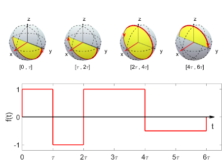
Figure 1: Sequence of DCR. The driving field is $\Omega_{x}(t)=\Omega_{x}f(t)\cos(\omega t)$, where the signs of $f(t)$ denote a clockwise and counterclockwise rotation, respectively. The spin is rotated by $\pi$ in the periods $[0,\tau]$, $[\tau,2\tau]$, and $[4\tau,6\tau]$ ($\tau={2\pi}/{\Omega_{x}}$) under the rotating wave approximation, but by $2\pi$ in the period $[2\tau,4\tau]$.

Once we consider a real situation in a BEC experiment, the Hamiltonian for our model must include various noise sources in the laboratory and becomes

$$H_{n}(t) = c_{2}{\bf J}^{2}+\omega_{0}J_{z}+(\Omega_{x}+\epsilon)\cos(\omega t)J_{x}$$ (1)

$$+\gamma(b_{x}J_{x}+b_{y}J_{y}+b_{z}J_{z}).$$

where $\omega=\omega_{0}-\Delta_{BS}$ to satisfy the resonant condition, $b_{x,y,z}$ are the three components of a stray magnetic field in the laboratory. We also include explicitly the control error $\epsilon$ caused by the fluctuation of the radio-frequency or microwave power and the finite bandwidth of the control field. We note that the magnetic field noise and the control error are modeled as ensemble white noise, which implies that the stray magnetic field $b_{x,y,z}$ and the control error $\epsilon$ are fixed for a single experiment run but distribute randomly and uniformly from run to run, i.e., $b_{x,y,z}\in[-b_{c},b_{c}]$ and $\epsilon\in[-\epsilon_{c},\epsilon_{c}]$ with $b_{c}$ and $\epsilon_{c}$ the respective cutoff.

It is straightforward to obtain the effective Hamiltonian  Takegoshi et al. (2015) with the stray magnetic field and the control error in the rotating reference frame defined by $U_{R}$

$$H_{n} \approx \frac{\Omega_{x}}{2}J_{x}+\left[\frac{\epsilon}{2}+\left(\frac{\Omega_{x}}{4\omega}\right)\left(\gamma b_{z}+\frac{\Omega_{x}^{2}}{32\omega}\right)\right]J_{x}$$ (2)

$$+\left[\gamma b_{z}-\frac{\epsilon}{2}\left(\frac{\Omega_{x}}{4\omega}\right)\right]J_{z},$$

under the conditions $\{\gamma b_{c}/\Omega_{x},\epsilon_{c}/\Omega_{x},\Omega_{x}/\omega\}\ll 1$. We further write down the evolution operator $U_{n}=\exp{(-i\tau H_{n})}\approx$ $\exp{[-i\pi(1+\epsilon/\Omega_{x})J_{n}]}$ where $J_{n}\approx J_{x}+2\gamma b_{z}/\Omega_{x}J_{z}$. It is obvious that the relative error of rotation angle is $\theta_{\parallel}\approx\epsilon/\Omega_{x}$ and the relative error of rotation direction $\theta_{\perp}\approx 2\gamma b_{z}/\Omega_{x}$. Clearly, this imperfect naive rotation (NR) deviates linearly from an ideal $\pi$ pulse, due to the control error $\epsilon$ and the stray magnetic field $b_{z}$. The rotation error exceeds 1% if $\epsilon_{c}/\Omega_{x}\sim 1\%$ or $\gamma b_{c}/\Omega_{x}\sim 1\%$.

To realize a more precise $\pi$ rotation, we adopt the DCR, which is inspired by the dynamically corrected gate originally designed to suppress static noises, e.g., $b_{x,y,z}$ Khodjasteh and Viola (2009a, b); Khodjasteh et al. (2010); Wimperis (1994); West et al. (2010); Kestner et al. (2013); Wang et al. (2012); Rong et al. (2014); Zeng and Barnes (2018). It is straightforward to prove that the time-dependent control error is canceled as well by the specific DCR pulse sequence shown in Fig. 1. In fact, the evolution operator for the DCR cycle is $U_{DCR}\approx\exp{\{-i\pi[1+\theta_{\parallel}]J_{n}^{\prime}\}}$ with $\theta_{\parallel}\approx 7\Omega_{x}^{2}/(256\omega^{2})+\gamma b_{z}/(2\omega)-4\pi(\gamma b_{z}/\Omega_{x})^{2}$ and $J_{n}^{\prime}=J_{x}-(4\pi\gamma b_{z}\epsilon/\Omega_{x}^{2})J_{y}+[4\pi\gamma b_{z}\epsilon/\Omega_{x}^{2}-\epsilon/(4\omega)]J_{z}$. One immediately finds $\theta_{\parallel}$ and $\theta_{\perp}$ are smaller than that in the NR, indicating the DCR is more accurate (see in Append. A).

To verify the above analytical results from the Magnus expansion theory, we carry out numerical simulations with the time-dependent Hamiltonian Eq. (1). For the DCR, the driving amplitude $\Omega_{x}$ (and the corresponding Bloch-Siegert shift $\Delta_{BS}$) becomes time-dependent as shown in Fig. 1. Since the relative fluctuation $|\Delta J_{\perp}/\langle{\mathbf{J}}\rangle|=1/\sqrt{N}=1\%$ for a coherent spin state with $N=10^{4}$, it is impossible to justify the high accuracy of the DCR. We thus employ an SSS whose relative fluctuation is in the order of $1/N=0.01\%$ Kitagawa and Ueda (1993a); Degen et al. (2017); Ma et al. (2011). Initially, we set the average spin $J_{0}=\langle{\bf J}\rangle$ along $-y$-axis and the optimal squeezing direction along $z$ direction. Once the NR or DCR pulses are finished, we calculate the observables $\langle J_{z}\rangle$ and $\Delta J_{z}=\sqrt{\langle J_{z}^{2}\rangle-\langle J_{z}\rangle^{2}}$. The rotation error (precision) is measured by the ratio of the two experimental observables to the average spin $J_{0}$ which should point along $y$-axis after the rotation. $\langle J_{z}\rangle/J_{0}$ denotes the deviation of the spin direction from the ideal one, and $\Delta J_{z}/J_{0}$ the quantum fluctuation of the spin. We note that the spin fluctuation along $x$ direction, $\Delta J_{x}$, is very large (in the order of $N$) and not useful in quantum sensing.

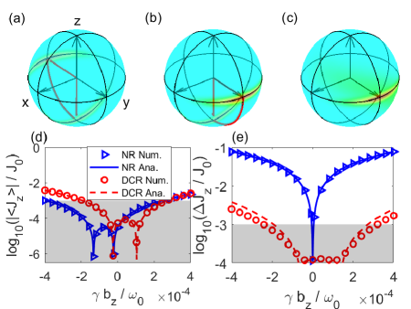
Figure 2: Rotation of the SSS. (a) The initial state with the average spin along $-y$-axis and the optimal squeezing in $z$ direction is rotated around $x$-axis. (b) The SSS is rotated to the final $y$ direction. (c) Comparison of the ideal SSS and the evolved final state with error. (d) Dependence of the average spin direction deviation on the magnetic field noise $b_{z}$. (e) Spin fluctuation. Panels (d) and (e) show numerical results after NR (blue triangles) and DCR (red circles), and analytical results after NR (blue solid line) and DCR (red dashed line). Other parameters are $N=10^{4}$, $\omega_{0}=\gamma B_{0}$ with $B_{0}=1$ G, $b_{x,y}=0$, $\epsilon=0$, and $J_{0}\approx 0.58N$.

We compare the NR and DCR of the condensate spin at different stray field $b_{z}$ in Fig. 2. We have set $b_{x,y}=0$ and $\epsilon=0$ for a clear comparison. For the spin average, $\langle J_{z}\rangle/J_{0}$, we observe that the deviation from the ideal direction is below 0.1% if the magnetic field noise is within 0.2 mG, either for the NR or the DCR. For the spin fluctuation $\Delta J_{z}/J_{0}$, the minima of both the NR and the DCR are close to the initial value of $1/N$. However, the DCR performs much robust against the field noise than the NR in general. To reach the precision of 0.1%, the DCR requires the magnetic noise below 0.2 mG but the NR requires much smaller noise. As shown also in Fig. 2 the numerical results are in good agreement with the analytical ones. It is lengthy but straightforward to obtain the analytical results for $\langle J_{z}\rangle/J_{0}$ and $\Delta J_{z}/J_{0}$ (Details of the derivation are in Append. A).

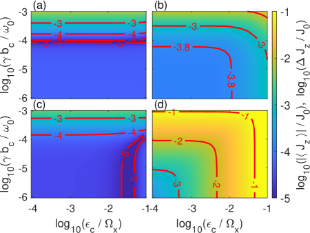
Figure 3: (a) Deviation of the spin direction $\log_{10}(|\langle J_{z}\rangle|/J_{0})$ and (b) spin fluctuation $\log_{10}(\Delta J_{z}/J_{0})$ after the DCR with an initial SSS. (c) and (d) are the same but after the NR. Obviously, the DCR performs more robust against the stray field noise and the control error than the NR, both for the deviation of the spin direction and for the spin fluctuation. Under realistic experiment conditions $b_{c}\sim 0.1$ mG (i.e., $\gamma b_{c}/\omega_{0}\sim 10^{-4}$) and $\epsilon/\Omega_{x}\sim 0.01$, the precision of the DCR is well below 0.1%. Each datum is averaged over $10^{6}$ random realizations.

In Fig. 3 we present numerical results of the deviation of the spin direction and the spin fluctuation after the DCR for various cutoff noise strength $b_{c}$ and control error $\epsilon_{c}$. For comparison, we also show the same results after the NR. As illustrated in Fig. 3(a) and (b), the deviation of the spin direction and the spin fluctuation are small with the stray field noise and the control error. In particular, they are both below 0.1% if the control error is smaller than $0.01\Omega_{x}$ and the stray field within 0.1 mG. However, the NR errors shown in Fig 3(c) and (d) are rather large, making the NR impossible to estimate the fidelity beyond the standard quantum limit. This is why we adopt the DCR to take the quantum-entanglement advantage of the SSS. We note that the numerical results agree well with the analytical ones which are detailed in Append. A.

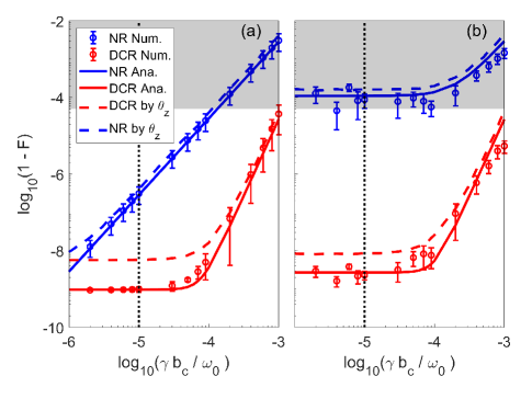
Figure 4: Dependence of the rotation infidelity $1-F$ on the cutoff of the stray magnetic field for (a) $\epsilon_{c}=0$ and (b) $\epsilon_{c}/\Omega_{x}=0.01$. In (a) and (b), the analytical results (solid lines) agree well with the numerical ones (circles with error bars) for DCR (lower) and NR (upper). The dashed lines denote the estimated rotation infidelity by $\theta_{z}$ for DCR (lower) and NR (upper). Each numerical datum is averaged over $5$ runs of random fields and the standard deviation is denoted by error bars. The vertical and the horizontal boundaries mark the reported $b_{c}=0.01$ mG and the infidelity $1-F=5\times 10^{-5}$, respectively Rong et al. (2015).

III $O(1)$ benchmarking of a precise rotation

With such a robust and high precision DCR at hand, we compare it with other single-particle quantum operations. The precision of most quantum operations are usually characterized by the operation infidelity, $1-F$, with $F$ the fidelity between the ideal operation and the realized one. After an analytical derivation, we find the rotation infidelity

$$1-F=1-\left|\frac{\sin{(\frac{3\theta}{2})}}{3\sin{\frac{\theta}{2}}}\right|$$ (3)

where the fidelity $F=|\rm Tr(U^{\dagger}X)|/\sqrt{\rm Tr(U^{\dagger}U)\rm Tr(X^{\dagger}X)}$ with $U$ the evolution operator, $X$ the ideal $\pi$-rotation operator, and the rotation error $\theta$ defined by $\exp(-i\theta J_{n})=U^{\dagger}X$. The rotation infidelity, $1-F\approx\theta^{2}/3$ if $\theta\ll 1$. One immediately obtains the rotation infidelity once one knows $\theta$ which may be calculated theoretically, simulated numerically, or estimated (measured) experimentally (More details are in Append. B).

We present the rotation infidelity after the DCR (and the NR) in Fig. 4. The numerical results are simulated by evolving the system under the time-dependent Hamiltonian Eq. (1). The analytical ones are straightforwardly calculated with the time-independent effective Hamiltonian Eq. (2) and the application of the DCR pulse sequence. As shown in Fig. 4, the numerical and the analytical results agree well, implying that the effective Hamiltonian is an excellent approximation to the real one if the stray magnetic field and the control error are small. As the stray field decreases from $\sim 1$ mG, the rotation infidelity decreases sharply in the form of $\left({\gamma b_{c}}/{\omega_{0}}\right)^{2}$ for the NR and $\left({\gamma b_{c}}/{\omega_{0}}\right)^{4}$ for the DCR. At an extremely small stray field, the infidelity reaches a plateau which stems from the high order terms beyond the Bloch-Siegert shift. Compared to the NR, the rotation infidelity after the DCR is several orders of magnitude smaller if the stray magnetic field lies in the range $b_{c}\in[0.01,1]$ mG. In fact, the DCR infidelity at the most stable laboratory field $b_{c}\sim 0.01$ mG is roughly one thousandth times the reported lowest gate infidelity in Nitrogen-vacancy centers in diamond Eto et al. (2013); Rong et al. (2015), indicating the great potential of the spinor BEC systems in precise quantum operations.

Benchmarking such a small rotation infidelity is a big challenge. However, by noticing the independence of the small rotation error $\theta$ on the atom number $N$ for the DCR, we may make full use of the advantages of many-body entanglement states, e.g. spin squeezed states, to estimate (measure) $\theta$ precisely and calculate the single-particle rotation infidelity $1-F$ with Eq. (3). To estimate efficiently the small rotation error $\theta$, we suggest $\theta\approx\theta_{z}=J_{z}/J_{0}$ where $J_{z}$ after the DCR is measured experimentally for an initial SSS with optimal squeezing along $z$-axis. As illustrated in Fig. 4, the rotation infidelity derived from $\theta_{z}$ agrees well with that from $\theta$, except the region with extremely tiny rotation infidelity $1-F<10^{-8}$. Such a limitation originates from the spin squeezing limit of the quantum state, which is in the order of $1/(3N^{2})\sim 10^{-8}$ for $N=10^{4}$ Kitagawa and Ueda (1993a). This limitation may be lower than $10^{-8}$ by increasing the atom number in a spin-1 BEC.

We remark that only several measurements of the rotation error are enough to obtain a pretty good estimation of the rotation infidelity with the spin-squeezed quantum state, as shown in Fig. 4. This $O(1)$ measurement requirement greatly relieves the experimental efforts and contrasts sharply to the quantum process tomography and the randomized benchmarking, which require $O(1/(1-F)^{2})$ and $O(1/(1-F))$ (equivalent) measurements, respectively Rong et al. (2015); Wu et al. (2013). Such a huge benefit comes from the accurate estimation of the rotation error and thus the rotation infidelity with the spin-squeezed quantum state, manifesting the quantum supremacy of entangled quantum states over the separable ones. Of course, one may carry out more experimental measurements with the spin-squeezed state to benchmark even lower rotation infidelity beyond the spin squeezing limit $1/(3N^{2})$.

IV Conclusion and discussion

In conclusion, we propose an $O(1)$ benchmarking method for a precise single-spin rotation with the error derived from the precisely measured rotation error by utilizing a squeezed spin state. With analytical calculations and numerical simulations, we show that a DCR decouples almost perfectly a spin-1 BEC from its magnetic noise environment when performing a $\pi$ rotation. The rotation infidelity after a DCR approaches $10^{-8}$ for $10^{4}$ atoms at the lowest laboratory magnetic field noise of $\sim 0.01$ mG and a relative control error of $\sim 1\%$. For such a high-precision rotation, it is viable to benchmark it by only several measurements with a squeezed spin state in a spin-1 BEC. Although our example focuses on a precise $\pi$ rotation, the $O(1)$ benchmarking is in principle applicable to an arbitrary rotation with a squeezed spin state, which may be prepared in a spin-1 BEC or a many-qubit system like trapped ions, superconducting qubits, Nitrogen-vacancy centers and neutral atoms in optical tweezers Kitagawa and Ueda (1993b); Caves (1981); Wineland et al. (1992).

The preparation of a spin squeezed state under current experimental condition has been discussed theoretically Xu et al. (2017); Huang et al. (2021). We notice two recent advances in spinor BECs. (i) Zou et al. demonstrated spin squeezing in $10^{4}$ atoms 18 dB below the standard quantum limit (SQL) which is the limit for a coherent spin state Zou et al. (2018). (ii) Single-atom level counting was reported via a combination of Stern-Gerlach separation and fluorescence imaging Evrard et al. (2021). By adopting both techniques, it is possible to implement the $O(1)$ benchmarking in spinor BEC experiments, at least at the level of $1-F\sim 10^{-6}$ since the spin squeezing has not reached perfectly the Heisenberg limit (which is 40 dB below the SQL). In addition, entanglement states were generated and high fidelity rotations realized in Nitrogen-vacancy centers experiments Xu et al. (2017); Rong et al. (2015); Xie et al. (2021); Liu et al. (2011); Yang et al. (2012), indicating that our method may also be applicable in these many-qubit systems in principle, though the size of qubits is quite limited.

Appendix A The Average Hamiltonian

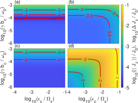
Figure 5: Same as Fig. 3 except for analytical results.

The spin-1 Bose-Einstein condensate (BEC) Hamiltonian under the single mode approximation is

$$H_{n}(t) = c_{2}{\bf J}^{2}+\omega_{0}J_{z}+(\Omega_{x}+\epsilon)\cos(\omega t)J_{x}$$ (4)

$$+\gamma(b_{x}J_{x}+b_{y}J_{y}+b_{z}J_{z}),$$

where $c_{2}<0$ is the ferromagnetic spin exchange coupling strength, $\omega_{0}=\gamma B_{0}$ is the Larmor frequency in a magnetic field $B_{0}$ with $\gamma$ the gyromagnetic ratio, $\Omega_{x}$ is the Rabi frequency of a RF field (carrier frequency $\omega$) coupled to the condensate atoms, and $J_{\alpha}=\sum_{i=1}^{N}s_{i\alpha}$ ($\alpha=x,y,z$) is the collective spin of the condensate with $s_{i\alpha}$ the atomic spin-1 matrix for the i-th atom and $N$ the total atom number. The control error $\epsilon$ and the magnetic field noise $b_{x,y,z}$ are fixed for a single experiment run, but they change for the next. In a typical spin-1 BEC experiment, $\{\gamma b_{x,y,z}/\Omega_{x},\epsilon/\Omega_{x},\Omega_{x}/\omega\}\ll 1$.

By employing a rotating reference frame defined by $U_{R}=\exp{\{-it(\omega J_{z}+c_{2}{\bf J}^{2})}$, the Hamiltonian becomes

$$H_{R}(t) = \gamma b_{z}J_{z}+[(\Omega_{x}+\epsilon)\cos(\omega t)+\gamma b_{x}]$$ (5)

$$\times[\cos(\omega t)J_{x}+\sin(\omega t)J_{y}]$$

$$+\gamma b_{y}[-\sin(\omega t)J_{x}+\cos(\omega t)J_{y}].$$

The average Hamiltonian with Magnus expansion to the second order in a period of $\tau_{0}=2\pi/\omega$ is Takegoshi et al. (2015)

$$\overline{H}_{n} \approx \left(\frac{\Omega_{x}}{2}+\frac{\epsilon}{2}+\frac{\gamma b_{z}\Omega_{x}}{4\omega}+\frac{\Omega_{x}^{3}}{128\omega^{2}}\right)J_{x}$$ (6)

$$+(\gamma b_{z}-\frac{\epsilon\Omega_{x}}{8\omega})J_{z},$$

which is nothing but Eq. (2). Note that the Bloch-Siegert shift has been included and the third and higher order terms are neglected.

Next we consider the effective evolution operator for the pulse sequence, dynamically corrected rotation (DCR). The effective Hamiltonians $\overline{H}_{k}$ during $[k-1,k]\tau$ $(k=1,2,\cdots,6)$ are

$$\overline{H}_{1} = \overline{H}_{n},$$

$$\overline{H}_{2} \approx -\left(\frac{\Omega_{x}}{2}+\frac{\epsilon}{2}+\frac{\gamma b_{z}\Omega_{x}}{4\omega}+\frac{\Omega_{x}^{3}}{128\omega^{2}}\right)J_{x}$$

$$+(\gamma b_{z}-\frac{\epsilon\Omega_{x}}{8\omega})J_{z},$$

$$\overline{H}_{3,4} = \overline{H}_{n},$$

$$\overline{H}_{5,6} \approx -\left(\frac{\Omega_{x}}{4}+\frac{\epsilon}{2}+\frac{\gamma b_{z}\Omega_{x}}{8\omega}+\frac{\Omega_{x}^{3}}{1024\omega^{2}}\right)J_{x}$$ (7)

$$+(\gamma b_{z}-\frac{\epsilon\Omega_{x}}{16\omega})J_{z}.$$

It is straightforward to calculate the effective evolution operator for the DCR

$$U_{DCR} = e^{(-i2\tau\overline{H}_{5})}e^{(-i2\tau\overline{H}_{1})}e^{(-i\tau\overline{H}_{2})}e^{(-i\tau\overline{H}_{1})}$$

$$\approx e^{\left[-i\pi(1+\theta_{\parallel})J_{\bf n}\right]},$$

with

$$\theta_{\parallel} = \frac{7\Omega_{x}^{2}}{256\omega^{2}}+\frac{\gamma b_{z}}{2\omega}-\frac{4\pi(\gamma b_{z})^{2}}{\Omega_{x}^{2}},$$

$$J_{\bf n} = J_{x}-\frac{4\pi\gamma b_{z}\epsilon}{\Omega_{x}^{2}}J_{y}+\left(\frac{4\pi\gamma b_{z}\epsilon}{\Omega_{x}^{2}}-\frac{\epsilon}{4\omega}\right)J_{z}.$$

Again we have neglected the third and higher order terms.

With the evolution operator above, one can straightforwardly calculate experimental observables, such as the spin average $\langle{J_{i}}\rangle=\text{Tr}\left(\rho_{0}U^{\dagger}{J_{i}}U\right)$ and its fluctuation $\Delta{J_{i}}=\sqrt{\text{Tr}\left(\rho_{0}U^{\dagger}{J_{i}^{2}}U\right)-\langle{J_{i}}\rangle^{2}}$ with $i=x,y,z$ for an initial spin state $\rho_{0}$. The results with $\epsilon=0$ are shown in Fig. 2, which agree well with the numerical ones. The results with $\epsilon\neq 0$ are shown in Fig. 5, which are also close to the numerical ones shown in Fig. 3.

Appendix B Rotation Infidelity

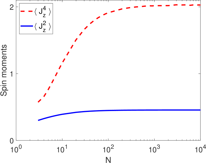
Figure 6: The minimum spin moments of $\langle J_{z}^{2}\rangle$ and $\langle J_{z}^{4}\rangle$ as a function of particle number $N$ for an optimal two-axis spin squeezed state.

Same as a quantum gate fidelity Wang et al. (2008), the rotation fidelity for a spin-1 BEC is defined as

$$F_{N} = \frac{\left|\text{Tr}\left(U^{\dagger}X\right)\right|}{2N+1}=\left|\frac{\sin\left(\left(2N+1\right)\frac{\theta}{2}\right)}{(2N+1)\sin\left(\frac{\theta}{2}\right)}\right|$$ (9)

where $U=U_{NR}=\exp{(-i\tau\overline{H}_{n})}$ for the NR, $U=U_{DCR}$ for the DCR, and $X=\exp{({-i\pi J_{x}})}$ for an ideal $\pi$ rotation operator around the $x$-axis. We have used that the product of two rotation operators is also a rotation operator, i.e., $U^{{\dagger}}X=\exp(-i\theta J_{n})$ with $J_{n}$ and $\theta$ given by

$$J_{n} = \frac{1}{\sin(\theta/2)}\left(\cos{\frac{\phi}{2}}J_{x}-c\sin{\frac{\phi}{2}}J_{y}+b\sin{\frac{\phi}{2}}J_{z}\right),$$

$$\cos\left(\frac{\theta}{2}\right) = a\sin\left(\frac{\phi}{2}\right),$$

for a rotation operator $U=\exp(-i\phi J_{\phi})$ and $J_{\phi}=aJ_{x}+bJ_{y}+cJ_{z}$ with $a^{2}+b^{2}+c^{2}=1$.

To fairly compare with single atom’s rotation fidelity in other systems, it is easy to derive the rotation fidelity for a single spin-1 atom from Eq. (9), by setting $N=1$,

$$F=\frac{2\cos{\theta}+1}{3}\approx 1-\frac{\theta^{2}}{3}$$ (10)

if $\theta$ is small. From the above function, one immediately obtains the average and the fluctuation of the rotation fidelity

$$F_{\rm avg} = \overline{1-\theta^{2}/3}=1-\frac{(\Delta\theta)^{2}+(\bar{\theta}\,)^{2}}{3},$$ (11)

$$(\Delta F)^{2} = \frac{1}{9}\left[\overline{\theta^{4}}-(\overline{\theta^{2}}\;)^{2}\right]$$ (12)

$$= \frac{1}{9}\left[\overline{\theta^{4}}-\left((\Delta\theta)^{2}+(\bar{\theta}\,)^{2}\right)^{2}\right]$$

where $\bar{x}$ is the average of $x$. To calibrate the infidelity to an accuracy $\varepsilon\ll 1$, we need to guarantee that $1-F_{\rm avg}<\varepsilon$ and $\Delta F<\varepsilon$. As shown in the above equation, $1-F_{\rm avg}$ and $\Delta F$ depends solely on the small error angle $\theta$ which can be estimated experimentally.

To accurately measure the error angle $\theta$, one may take advantage of the squeezed spin state (SSS) in a spin-1 BEC. A crude estimation is $\theta\approx\theta_{z}=J_{z}/J_{0}$ for the designed initial SSS. Under this approximation, we find

$$F_{\rm avg} = 1-\frac{(\Delta J_{z})^{2}+\langle J_{z}\rangle^{2}}{3J_{0}^{2}},$$

$$\Delta F = \frac{1}{3J_{0}^{2}}\;\sqrt{\langle J_{z}^{4}\rangle-\left[(\Delta J_{z})^{2}+\langle J_{z}\rangle^{2}\right]^{2}}\quad.$$ (13)

The spin moments above can be measured precisely in experiments. It is well known that, for an optimal SSS with $N$ atoms, $\Delta J_{z}/J_{0}\sim 1/N$ and $\langle J_{z}\rangle=0$ with optimal squeezing along $z$-axis Kitagawa and Ueda (1993b).

For the optimal SSS we employ, we calculate the moments of the condensate spin $J_{z}$. As shown in Fig. 6, $\langle J_{z}\rangle=0$, $\langle J_{z}^{2}\rangle\approx 0.5$, and $\langle J_{z}^{4}\rangle\approx 2$ for $N>10^{2}$. From Eq. (B) one immediately finds that $1-F_{\rm avg}$ and $\Delta F$ are both in the order of $1/N^{2}$, indicating that $O(1)$ benchmarking at the level of $1/N^{2}$ is possible if other noises, such as the stray magnetic field and the control error, are well under control with the DCR.

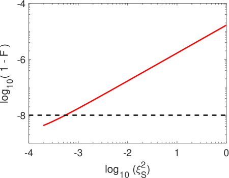
Figure 7: Dependence of infidelity on spin squeezing parameters. The horizontal dashed line denotes the value of $1-F=1/N^{2}$ with $N=10^{4}$.

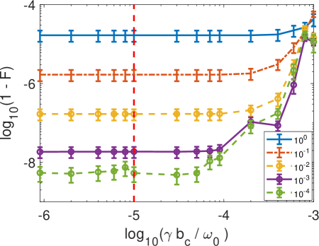
Figure 8: Dependence of infidelity on stray magnetic noises with relative control error $\epsilon_{c}/\Omega_{x}=0.01$ after DCR. The spin squeezing parameter of initial SSS are $1$ (blue solid line), $10^{-1}$ (red dash-dotted line), $10^{-2}$ (yellow dashed line with circles), $10^{-3}$ (purple solid line with circles), $10^{-4}$ (green dashed line with circles), from top to bottom. Each datum is averaged over $5$ random realizations and the error bars are the standard deviation (halved for a clear view). The vertical red dashed line marks the position $b_{c}=0.01$ mG.

In real experiments, initial state often deviates from the optimal SSS. According to Eq. (B), the infidelity after a perfect rotation is

$$1-F_{\rm avg}=\frac{N\xi_{S}^{2}}{6J_{0}^{2}},$$ (14)

in the case of zero stray magnetic noises (thus $\langle J_{z}\rangle=0$). The spin squeezing parameter $\xi_{S}^{2}=(\Delta J_{z})^{2}/(N/2)$ was originally introduced by Kitagawa and Ueda Kitagawa and Ueda (1993a). The result is plotted in Fig. 7. As shown clearly in the figure, the infidelity reaches $\sim 1/N^{2}$ when $\xi_{S}^{2}$ is smaller than $10^{-3}$. With the presence of magnetic noise and control error, numerical simulations of initial states with various $\xi_{S}^{2}$ are shown in Fig. 8. Obviously, the infidelities at small noises agree well with the prediction of Eq. (14), indicating that $O(1)$ benchmarking is possible if the squeezing parameter is smaller than $10^{-3}$.

To estimate $\theta$ more accurately, one may repeat the experiment to measure $\theta_{n}$ with the optimal squeezing axis of the initial SSS along different directions. In this way, the rotation fidelity becomes more accurate. However, it still scales as $1/N^{2}$.

To calibrate an arbitrary rotation $R(\alpha,{\bf k})$ with $\alpha$ the rotation angle and ${\bf k}$ the rotation axis, one may prepare the initial SSS under the conditions both ${\bf n}_{0}\perp{\bf k}$ and ${\bf s}_{0}\perp{\bf k}$ where ${\bf n}_{0}$ and ${\bf s}_{0}$ are the average spin direction and the optimal squeezing direction of the initial state. Here $R(\alpha,{\bf k})$ stands for a $3\times 3$ special orthogonal rotation matrix. Correspondingly, the measurement direction becomes ${\bf s}_{f}=R(\alpha,{\bf k}){\bf s}_{0}$ after the rotation.

References

- Nielsen and Chuang (2002) M. A. Nielsen and I. Chuang, Am. J. Phys. 70, 558 (2002).
- Giovannetti et al. (2004) V. Giovannetti, S. Lloyd, and L. Maccone, Science 306, 1330 (2004).
- Xu et al. (2019) P. Xu, S. Yi, and W. Zhang, Phys. Rev. Lett. 123, 073001 (2019).
- Ma et al. (2011) J. Ma, X. Wang, C. Sun, and F. Nori, Phys. Rep. 509, 89 (2011).
- Bao et al. (2020) H. Bao, J. Duan, S. Jin, X. Lu, P. Li, W. Qu, M. Wang, I. Novikova, E. E. Mikhailov, K. F. Zhao, K. Mølmer, H. Shen, and Y. Xiao, Nature 581, 159 (2020).
- Duan et al. (2000) L.-M. Duan, A. Sørensen, J. I. Cirac, and P. Zoller, Phys. Rev. Lett. 85, 3991 (2000).
- Pu and Meystre (2000) H. Pu and P. Meystre, Phys. Rev. Lett. 85, 3987 (2000).
- Gaebler et al. (2012a) J. P. Gaebler, A. M. Meier, T. R. Tan, R. Bowler, Y. Lin, D. Hanneke, J. D. Jost, J. P. Home, E. Knill, D. Leibfried, and D. J. Wineland, Phys. Rev. Lett. 108, 260503 (2012a).
- Kawakami et al. (2016) E. Kawakami, T. Jullien, P. Scarlino, D. R. Ward, D. E. Savage, M. G. Lagally, V. V. Dobrovitski, M. Friesen, S. N. Coppersmith, M. A. Eriksson, and L. M. K. Vandersypen, Proc. Natl. Acad. Sci. USA 113, 11738 (2016).
- Fogarty et al. (2015) M. A. Fogarty, M. Veldhorst, R. Harper, C. H. Yang, S. D. Bartlett, S. T. Flammia, and A. S. Dzurak, Phys. Rev. A 92, 022326 (2015).
- Levine et al. (2019) H. Levine, A. Keesling, G. Semeghini, A. Omran, T. T. Wang, S. Ebadi, H. Bernien, M. Greiner, V. Vuletić, H. Pichler, and M. D. Lukin, Phys. Rev. Lett. 123, 170503 (2019).
- Nemirovsky and Sagi (2021) J. Nemirovsky and Y. Sagi, Phys. Rev. Res. 3, 013113 (2021).
- Bowdrey et al. (2002) M. D. Bowdrey, D. K. Oi, A. Short, K. Banaszek, and J. Jones, Phys. Lett. A 294, 258 (2002).
- Wang et al. (2008) X. Wang, C.-S. Yu, and X. Yi, Phys. Lett. A 373, 58 (2008), ISSN 0375-9601.
- Nielsen (2002) M. A. Nielsen, Phys. Lett. A 303, 249 (2002).
- Wu et al. (2013) Z. Wu, S. Li, W. Zheng, X. Peng, and M. Feng, J. Chem. Phys 138, 024318 (2013).
- Knill et al. (2008) E. Knill, D. Leibfried, R. Reichle, J. Britton, R. B. Blakestad, J. D. Jost, C. Langer, R. Ozeri, S. Seidelin, and D. J. Wineland, Phys. Rev. A 77, 012307 (2008).
- Zhang et al. (2016) C. Zhang, X.-C. Yang, and X. Wang, Phys. Rev. A 94, 042323 (2016).
- Gaebler et al. (2012b) J. P. Gaebler, A. M. Meier, T. R. Tan, R. Bowler, Y. Lin, D. Hanneke, J. D. Jost, J. P. Home, E. Knill, D. Leibfried, and D. J. Wineland, Phys. Rev. Lett. 108, 260503 (2012b).
- Sheng et al. (2018) C. Sheng, X. He, P. Xu, R. Guo, K. Wang, Z. Xiong, M. Liu, J. Wang, and M. Zhan, Phys. Rev. Lett. 121, 240501 (2018).
- Stamper-Kurn and Ueda (2013) D. M. Stamper-Kurn and M. Ueda, Rev. Mod. Phys. 85, 1191 (2013).
- Kawaguchia and Uedaa (2012) Y. Kawaguchia and M. Uedaa, Phys. Rep. 520, 253 (2012).
- Law et al. (1998) C. K. Law, H. Pu, and N. P. Bigelow, Phys. Rev. Lett. 81, 5257 (1998).
- Yi et al. (2002) S. Yi, O. E. Müstecaplıoğlu, C. P. Sun, and L. You, Phys. Rev. A 66, 011601(R) (2002).
- Hamley et al. (2012) C. D. Hamley, C. S. Gerving, T. M. Hoang, E. M. Bookjans, and M. S. Chapman, Nat. Phys. 8, 305 (2012).
- Xu et al. (2017) P. Xu, H. Sun, S. Yi, and W. Zhang, Sci. Rep. 7, 14102 (2017).
- Luo et al. (2017) X. Y. Luo, Y. Q. Zou, L. N. Wu, Q. Liu, M. F. Han, M. K. Tey, and L. You, Science 355, 620 (2017).
- Bloch and Siegert (1940) F. Bloch and A. Siegert, Physical Review 57, 522 (1940).
- Takegoshi et al. (2015) K. Takegoshi, N. Miyazawa, K. Sharma, and P. K. Madhu, J. Chem. Phys. 142 (2015).
- Khodjasteh and Viola (2009a) K. Khodjasteh and L. Viola, Phys. Rev. Lett. 102, 080501 (2009a).
- Khodjasteh and Viola (2009b) K. Khodjasteh and L. Viola, Phys. Rev. A 80, 032314 (2009b).
- Khodjasteh et al. (2010) K. Khodjasteh, D. A. Lidar, and L. Viola, Phys. Rev. Lett. 104, 090501 (2010).
- Wimperis (1994) S. Wimperis, J. Magn. Reson., Ser. A 109, 221 (1994).
- West et al. (2010) J. R. West, D. A. Lidar, B. H. Fong, and M. F. Gyure, Phys. Rev. Lett. 105, 230503 (2010).
- Kestner et al. (2013) J. P. Kestner, X. Wang, L. S. Bishop, E. Barnes, and S. Das Sarma, Phys. Rev. Lett. 110, 140502 (2013).
- Wang et al. (2012) X. Wang, L. S. Bishop, J. Kestner, E. Barnes, K. Sun, and S. Das Sarma, Nat. Commun. 3, 997 (2012).
- Rong et al. (2014) X. Rong, J. Geng, Z. Wang, Q. Zhang, C. Ju, F. Shi, C.-K. Duan, and J. Du, Phys. Rev. Lett. 112, 050503 (2014).
- Zeng and Barnes (2018) J. Zeng and E. Barnes, Phys. Rev. A 98, 012301 (2018).
- Kitagawa and Ueda (1993a) M. Kitagawa and M. Ueda, Phys. Rev. A 47, 5138 (1993a).
- Degen et al. (2017) C. L. Degen, F. Reinhard, and P. Cappellaro, Rev. Mod. Phys. 89, 035002 (2017).
- Rong et al. (2015) X. Rong, J. Geng, F. Shi, Y. Liu, K. Xu, W. Ma, F. Kong, Z. Jiang, Y. Wu, and J. Du, Nat. Commun. 6 (2015).
- Eto et al. (2013) Y. Eto, H. Ikeda, H. Suzuki, S. Hasegawa, Y. Tomiyama, S. Sekine, M. Sadgrove, and T. Hirano, Phys. Rev. A 88, 031602(R) (2013).
- Kitagawa and Ueda (1993b) M. Kitagawa and M. Ueda, Phys. Rev. A 47, 5138 (1993b).
- Caves (1981) C. M. Caves, Phys. Rev. D 23, 1693 (1981).
- Wineland et al. (1992) D. J. Wineland, J. J. Bollinger, W. M. Itano, F. L. Moore, and D. J. Heinzen, Phys. Rev. A 46, R6797 (1992).
- Huang et al. (2021) L.-G. Huang, F. Chen, X. Li, Y. Li, R. Lü, and Y.-C. Liu, NPJ Quantum Inf. 7, 168 (2021).
- Zou et al. (2018) Y. Q. Zou, L. N. Wu, Q. Liu, X. Y. Luo, S. F. Guo, J. H. Cao, M. K. Tey, and L. You, Proc. Natl Acad. Sci. 115, 6381 (2018).
- Evrard et al. (2021) B. Evrard, A. Qu, J. Dalibard, and F. Gerbier, Science 373, 1340 (2021).
- Xie et al. (2021) T. Xie, Z. Zhao, X. Kong, W. Ma, M. Wang, X. Ye, P. Yu, Z. Yang, S. Xu, P. Wang, Y. Wang, F. Shi, and J. Du, Sci. Adv. 7, eabg9204 (2021).
- Liu et al. (2011) Y. C. Liu, Z. F. Xu, G. R. Jin, and L. You, Phys. Rev. Lett. 107, 013601 (2011).
- Yang et al. (2012) W. L. Yang, Z. Q. Yin, Q. Chen, C. Y. Chen, and M. Feng, Phys. Rev. A 85, 022324 (2012).