Interpretable Survival Analysis for Heart Failure Risk Prediction

Abstract

Survival analysis, or time-to-event analysis, is an important and widespread problem in healthcare research. Medical research has traditionally relied on Cox models for survival analysis, due to their simplicity and interpretability. Cox models assume a log-linear hazard function as well as proportional hazards over time, and can perform poorly when these assumptions fail. Newer survival models based on machine learning avoid these assumptions and offer improved accuracy, yet sometimes at the expense of model interpretability, which is vital for clinical use. We propose a novel survival analysis pipeline that is both interpretable and competitive with state-of-the-art survival models. Specifically, we use an improved version of survival stacking to transform a survival analysis problem to a classification problem, ControlBurn to perform feature selection, and Explainable Boosting Machines to generate interpretable predictions. To evaluate our pipeline, we predict risk of heart failure using a large-scale EHR database. Our pipeline achieves state-of-the-art performance and provides interesting and novel insights about risk factors for heart failure.

1 Introduction

Predicting individualized risk of developing a disease or condition, e.g. heart failure, is a classical and important problem in medical research. While this risk modeling is sometimes accomplished using classification models, healthcare data often contains many right-censored samples: patients who are lost to followup before the end of the prediction window. Classification models cannot directly handle such censored data; instead, these samples are often discarded, losing valuable signal. Moreover, the classification approach requires fixing a specific risk window (e.g., whether a patient has developed heart failure in the first five years after their initial visit), and cannot exploit the time-to-event signal.

Survival analysis, in contrast, handles right-censoring by modeling the time until a patient develops a condition as a continuous random variable $T$ in order to estimate the survival curve $P(T>t)$. Survival analysis tasks have typically been modeled using Cox proportional hazards models (Cox, 1972), which assume that the log of the hazard function is a linear function of patient covariates plus a time-dependent intercept, resulting in proportional hazards over time. Cox models account for right-censored data by optimizing the partial likelihood

$$L(\beta)=\prod_{i=1}^{K}\frac{\exp(x_{i}^{\top}\beta)}{\sum_{j\in R(t_{i})}\exp(x_{j}^{\top}\beta)},$$ (1)

where $K$ denotes the number of uncensored event times $t_{1}\leq t_{2}\leq\cdots\leq t_{K}$ and $R(t_{i})=\{j:t_{j}\geq t_{i}\}$ represents the risk set of patients that have not passed away yet at time $t_{i}$. Since the sum in the denominator of Eq. (1) is over all patients in $R(t_{i})$ regardless of censoring, Cox models can learn signal from both censored and uncensored patients. Cox models have become the standard in survival analysis due to their simplicity, interpretability, and natural handling of time-to-event data with censoring.

Naturally, the machine learning community has proposed many models that improve risk prediction accuracy past Cox models. For example, the package scikit-survival (Pölsterl, 2020) contains several machine learning models for survival analysis, most of which do not assume a log-linear hazard function. Further, some recent machine learning approaches deal with right-censored data by adopting pseudovalues or pseudo-observations (Andersen and Pohar Perme, 2010), which requires that an estimator for the survival curve on the complete data is available, e.g. through the Kaplan-Meier estimator. Pseudovalues have enabled researchers to use machine learning regression models for survival analysis, further increasing the role of machine learning in the community.

One application of such survival analysis methods is heart failure risk prediction (Chicco and Jurman, 2020; Newaz et al., 2021; Fahmy et al., 2021; Panahiazar et al., 2015). Heart failure occurs when the heart loses the ability to relax or contract normally, leading to higher pressures within the heart or the inability to provide adequate output to the body. Heart failure is projected to affect over 6 million individuals in the U.S., is often fatal (i.e., it is mentioned in 13.4% of death certificates), and costs society over 30 billion dollars, all in the United States alone (CDC, 2023). Luckily, heart failure can often be prevented with preventive therapy if those at high risk can be identified in advance (Tsao et al., 2022). Machine learning models can help identify those at high risk better than traditional survival analysis models by offering improved discrimination. Nonetheless, one of the main roadblocks preventing machine learning approaches from becoming widely adopted in medical practice, including in heart failure risk prediction, is their black-box nature.

Interpretable machine learning methods hold the promise of delivering both high accuracy and interpretability, and thus have the potential to promote the adoption of machine learning methods in practice. Post-hoc explainability methods such as SHapley Additive exPlanations (SHAP) (Lundberg and Lee, 2017) and Local Interpretable Model-agnostic Explanations (LIME) (Ribeiro et al., 2016) are widely used, but provide potentially limited intelligibility as post-hoc methods (Kumar et al., 2020; Van den Broeck et al., 2022; Alvarez-Melis and Jaakkola, 2018; Rahnama and Boström, 2019). Further, Explainable Boosting Machines (Lou et al., 2013) have gained popularity due to their inherent interpretability as a generalized additive model (Hastie, 2017) and state-of-the-art accuracy.

To handle right-censored data, learn from time-to-event signal, and increase model interpretability, we present a complete pipeline to perform interpretable survival analysis without the need to estimate survival times. Specifically, we present an improved, scalable version of survival stacking (Craig et al., 2021), which generates classification training samples from the risk sets of the underlying survival analysis problem without having to estimate survival times (like pseudovalues do). Additionally, to reduce feature correlation that can hurt interpretability, we use ControlBurn (Liu et al., 2021) for (nonlinear) feature selection. ControlBurn prunes a forest of decision trees, thereby selecting important risk factors from a potentially large collection of candidate features. After survival stacking and feature selection, we use Explainable Boosting Machines (Lou et al., 2013) to generate trustworthy yet accurate survival predictions with both global and local explanations.

To evaluate our pipeline, we study heart failure risk prediction using electronic health record (EHR) data from a large hospital network with over 350,000 patients. Our experimental results show that our pipeline can predict heart failure more accurately than traditional survival analysis models and is comparable to other state-of-the-art machine learning models, while providing intelligibility. Our models both validate known risk factors for incident heart failure and identify novel risk factors.

2 Related Work

Several previous works have explored nonlinear extensions to classical survival models such as Cox proportional hazards models. A popular approach is to use the Cox partial likelihood as a loss function for common machine learning models, such as generalized additive models (Hastie and Tibshirani, 1995; Utkin et al., 2022), boosting (Ridgeway, 1999), support vector machines (Van Belle et al., 2007), and deep neural networks (Katzman et al., 2018). While generalized additive models are interpretable, using the Cox partial likelihood inherently enforces a proportional hazards assumptions, which might not be met in practice. Other works discard the proportional hazards assumption and instead use machine learning methods to estimate the survival curve, popular examples including Random Survival Forests (Ishwaran et al., 2008), RNN-Surv (Giunchiglia et al., 2018), and DeepHit (Lee et al., 2018). However, these models’ lack of interpretability is a challenge for implementation in clinical practice.

Other related works have explored casting survival analysis to a binary classification or regression problem. Most notably, the use of pseudo-values (Andersen and Pohar Perme, 2010) enables converting a survival analysis problem to a regression problem by directly predicting Kaplan-Meier estimates of the survival curve. Using pseudo-values does not require a proportional hazards assumption, and has been paired with various regression models in previous works (Rahman et al., 2021; Zhao and Feng, 2019; Rahman and Purushotham, 2022b, a; Feng and Zhao, 2021). Perhaps most similar to our paper, PseudoNAM (Rahman and Purushotham, 2021) combines pseudo-values with Neural Additive Models (Agarwal et al., 2021) for interpretable survival analysis. While PseudoNAM provides a straightforward solution for interpretable survival analysis (but without potentially important interaction terms), it could be biased when censoring is not independent of the covariates (Binder et al., 2014), a common situation in medical applications that censor on death. Instead of pseudo-values, our paper uses survival stacking (Craig et al., 2021) to cast survival analysis as a classification problem, which avoids such bias.

3 Methods

We present a complete pipeline for interpretable and accurate survival analysis. We use improved survival stacking, feature selection via ControlBurn (Liu et al., 2021), and interpretable classification via Explainable Boosting Machines (Lou et al., 2013) for our pipeline, which is summarized in Figure 1. We present each part of our pipeline in more detail in the proceeding subsections. For more background on survival analysis, see Appendix A.

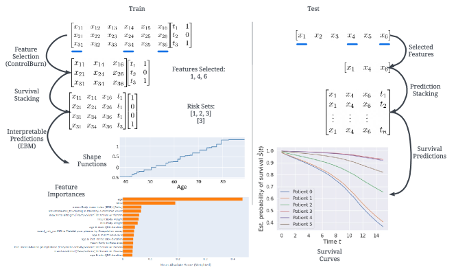
Figure 1: A summary of our interpretable survival analysis pipeline. During training (left), we use ControlBurn for feature selection (Section 3.3), survival stacking with subsampling to cast the survival data to classification data (Algorithm 1), and EBMs for generating feature importances and shape plots (Section 3.2). At test time (right), we use Survival Prediction (Algorithm 2) to generate survival curves using the trained ControlBurn and EBM models.

3.1 Survival Stacking

As discussed in Section 1, survival analysis is often a better solution for risk prediction than fixed-time classification, as survival analysis naturally handles censoring and incorporates time-to-event signal. However, much more research in machine learning, including interpretable machine learning, has focused on classification models. Thus, casting a survival analysis problem to an equivalent classification problem would enable the use of such state-of-the-art classification models.

We describe an improved version of survival stacking (Craig et al., 2021) that allows for the use of binary classification models for survival analysis. We assume survival data $\{(X_{i},T_{i},\delta_{i})\}_{i=1}^{n}$ where $X_{i}$ is a vector of covariates, $T_{i}$ is the time when the event of interest occurs (e.g. getting heart failure), and $\delta_{i}$ is the censoring indicator, indicating whether, at time $T_{i}$, patient $i$ reaches the event of interest or is lost to future observation before developing the condition. For each event time $t$ observed in the original data set, survival stacking adds all samples $X_{i}$ in the corresponding risk set $R(t)=\{i:T_{i}\geq t\}$ to a new “stacked” data set. For sample $i\in R(t)$, the corresponding binary label in the stacked data set is $0$ if $T_{i}>t$, and $1$ if $T_{i}=t$. Additionally, an extra covariate is added to the stacked data set representing the time $t$ which defines the risk set $R(t)$. Survival stacking works because training a binary classifier on the survival stacked data estimates the hazard function $\lambda(t\mid X)$ (the instantaneous risk conditioned on surviving until time $t$), which can be used to generate survival curves (see Appendix A). An example of survival stacking on a smaller data set can be found in (Craig et al., 2021).

We use an improved version of survival stacking in our pipeline, which is outlined in Algorithm 1. Specifically, we make two modifications to survival stacking as in (Craig et al., 2021) to better scale to large survival data sets. First, instead of defining a one-hot-encoded categorical variable to represent time, we define a single continuous time feature. This choice reduces the number of features, aiding computational efficiency and interpretability. Second, stacking increases the number of samples quadratically, potentially creating computational hardships as well as a severe class imbalance in the case of a high censoring rate. We perform random undersampling of the majority class samples $\{i:T_{i}>t\}\subset R(t)$ to mitigate this issue.

3.1.1 Survival Stacking Prediction

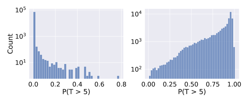
Figure 2: Distribution of predicted survival probabilities $S(t\mid X_{i})=P(T_{i}>t)$ at $t=5$ across test patients. The left plot shows the survival probabilities using Eq. (2) as in (Craig et al., 2021), while the right plot shows Eq. (5). Our survival prediction method gives a reasonable distribution, while the method from (Craig et al., 2021) is incorrectly skewed torwards 0.

After training a classification model $f$ on survival stacked data, we must convert the model’s predicted probabilities to survival curves for patients during inference. In (Craig et al., 2021), the survival curve $S(t\mid X)=P(T>t\mid X)$ is estimated using

$$\hat{S}(t\mid X)=\prod_{t_{k}\leq t}\Big{(}1-f(X\mathbin{\|}t_{k})\Big{)}.$$ (2)

where $\mathbin{\|}$ represents concatenation to add the extra time covariate from survival stacking. The motivation for Eq. (2) is that if the time variable $T$ is assumed to be discrete, taking on only the observed times $t_{1},\ldots,t_{k}$ in the training set, then, assuming without loss of generality $t_{1}\leq t_{2}\leq\cdots\leq t_{k}\leq t$, $S(t\mid X)$ can be written as the product of conditional survival probabilities up until time $t$:

$$S(t\mid X)=P(T>t\mid X)=\prod_{t_{k}\leq t}\Big{(}1-\lambda(t_{k}\mid X)\Big{)}$$ (3)

see Appendix LABEL:(Suresh et al., 2022) for details. This motivates Eq. (2) since the binary classifier $f$ estimates the hazard function $\lambda(t\mid X)$ with survival stacking. However, the estimate in Eq. (2) can become unstable in large sample, as demonstrated in Figure 2. Further, we use a continuous time feature in our survival stacking algorithm, implying that this discrete time assumption may not be suitable. Thus, we propose a different method for predicting the survival curve, which is summarized in Algorithm 2. We first predict the cumulative hazard function $\Lambda(t\mid X)=\int_{0}^{t}\lambda(s\mid X)ds$ using Monte Carlo integration at $n$ uniform continuously sampled times $t_{1},\ldots,t_{n}\leq t$:

$$\hat{\Lambda}(t\mid X)=\frac{t}{n}\sum_{i=1}^{n}f(X\mathbin{\|}t_{i}).$$ (4)

After estimating $\Lambda(t\mid X)$, we can naturally estimate $S(t\mid X)$ using

$$\hat{S}(t\mid X)=\exp\left(-\hat{\Lambda}(t\mid X)\right).$$ (5)

Using this estimator is possible since we used a continuous time feature in survival stacking, which allows for such Monte Carlo integration.

Algorithm 1 Survival Stacking With Subsampling

1:  Input: Survival data $(X_{1},T_{1},Y_{1}),\ldots,$           $(X_{n},T_{n},Y_{n})$, sampling ratio $\gamma$.

2:  Output: Classification data.

3:  $\text{event\_times}\leftarrow\{T_{i}:Y_{i}=1\}$, $\text{samples}\leftarrow[~{}]$.

4:  for $t$ in event_times do

5:     samples $\mathrel{+}=$ $\{(X_{i}\mathbin{\|}T_{i},1):T_{i}=t,Y_{i}=1\}$.

6:     risk_set = uniform random sample with               probability $\gamma$ from $\{i:T_{i}>t\}$.

7:     samples $\mathrel{+}=\{(X_{i}\mathbin{\|}T_{i},0):i\in\text{risk\_set}\}$.

8:  return  samples.

Algorithm 2 Survival Prediction

1:  Input: Fitted classification model $f$, survival data test sample $X$, prediction time $t$.

2:  Output: Estimated survival probability             $\hat{S}(t\mid X)=P(T>t\mid X)$.

3:  Sample $t_{1},\ldots,t_{n}$ uniformly from $(0,t]$.

4:  Estimate CHF via Monte Carlo integration:             $\hat{\Lambda}(t\mid X)=\frac{t}{n}\sum_{i=1}^{n}f(X\mathbin{\|}t_{i})$.

5:  return  $\hat{S}(t\mid X)=\exp(-\hat{\Lambda}(t\mid X))$.

3.2 Explainable Boosting Machines

Explainable Boosting Machines (EBMs) (Lou et al., 2012) are specific instances of Generalized Additive Models (GAMs) with interaction terms (Hastie, 2017; Lou et al., 2013):

$$\begin{split}g(\mathbb{E}[y])=\beta_{0}&+f_{1}(x_{1})+f_{2}(x_{2})+\cdots\\ &+f_{p}(x_{p})+\sum_{i,j}f_{i,j}(x_{i},x_{j}),\end{split}$$ (6)

where $g$ denotes a link function (e.g. identity for regression tasks and logistic for classification). The $f_{i}$’s are called the univariate shape functions, or ‘main effects’, whereas the $f_{i,j}$’s encode the interaction terms between features $x_{i}$ and $x_{j}$ and are known as the ‘interaction effects’ or ‘2D shape functions’. EBMs fit these shape functions by applying cyclic gradient boosting on shallow decision trees, see (Lou et al., 2013) for technical details. This process includes a crucial purification process (Lengerich et al., 2020) that ensures that each $f_{i}(x_{i})$ encodes the full and sole effects of feature $x_{i}$ to the target in the model, and similarly so for higher-order terms, so that they form a functional ANOVA decomposition. As a result, shape functions do not necessarily show marginalised effects, unlike partial dependence plots (PDPs). Without purification, encoding the sole effect is not guaranteed, as an identifiability issue would arise: the contribution of $x_{i}$ could be moved freely between its main effect and its interaction terms without changing the model predictions (Lengerich et al., 2020).

EBMs provide interpretability via the plotting of main effects and interaction terms, as well as feature importances by averaging the absolute contributions of a feature to the target over all samples (Nori et al., 2019). Perhaps surprisingly, EBMs achieve comparable performance to state-of-the-art tabular prediction methods while providing more interpretability (Nori et al., 2021; Lou et al., 2012; Kamath and Liu, 2021). They have been applied to a wide variety of fields, including high-risk applications in healthcare (Lengerich et al., 2022; Bosschieter et al., 2022; Sarica et al., 2021; Qu et al., 2022).

3.3 Feature Selection

One challenge for interpretable classification models is feature correlation, especially when the data set is high-dimensional. In particular, feature importance scores can be split between correlated features, resulting in potentially biased feature importance rankings (Liu et al., 2021). This problem is rather common in electronic health record (EHR) data, which often contains many highly correlated features. For example, healthcare data typically includes features for a patient’s height, weight, and BMI, which are highly correlated. Additionally, generating multiple features from a single feature’s time series, such as a patient’s average and last measured value of a lab test, typically resulting in correlated features. We thus consider feature selection as an important part in the interpretable survival analysis pipeline.

We choose to use ControlBurn (Liu et al., 2021) for feature selection, which is specifically designed to mitigate the bias induced by the correlated features. ControlBurn builds a forest of shallow trees and uses a LASSO model (Tibshirani, 1996) to prune trees, keeping only the features that are left in the unpruned trees. This process is similar to the traditional linear LASSO model, but is capable of capturing nonlinear relationships through ensembles of decision trees before pruning. ControlBurn has been shown to be efficient and outperform other feature selection methods on data with correlated features (Liu et al., 2021, 2022), making it a good option for large-scale healthcare data sets.

Since ControlBurn performs feature selection through classification, using the survival stacked data set discussed in Section 3.1 to perform feature selection is a natural choice. However, in some cases, it may be too computationally expensive to build the survival stacked data set before doing feature selection if both the number of samples and number of features are large. In such large data cases, a reasonable alternative is to fix a future time $t$ and perform feature selection using classification data at the fixed time $t$.

4 Experiments

4.1 Data

We evaluate our interpretable survival analysis pipeline through a large-scale study of incident heart failure risk prediction. Specifically, we gather EHR data from a large-scale hospital network (name censored for anonymity) for a total of $n=363,398$ patients and $p=1,590$ features. Additional information about cohort selection and characteristics are provided in Appendix B.

4.2 Setup

For preprocessing, we standardize continuous features across the observed entries and use mean imputation (equivalent to 0-imputation after standardization), while we use one-hot encoding for categorical features. Then, for feature selection, we contrast ControlBurn (discussed in Section 3.3) and linear LASSO (Tibshirani, 1996). We apply an 80/20 train-test split, and evaluate models with 5 trials each with different random seeds. The models we run are a Cox proportional hazards model (CoxPH, (Cox, 1972)), Random Survival Forest (RSF, (Ishwaran et al., 2008)), Logistic Regression (LogReg), XGBoost (Chen and Guestrin, 2016), and an Explainable Boosting Machine (EBM, (Lou et al., 2013; Nori et al., 2019)). Note that LogReg, XGBoost, and the EBM are fit on the stacked data built using Algorithm 1. All models are evaluated through the cumulative/dynamic AUC and integrated Brier score as defined in scikit-survival (Pölsterl, 2020).

4.3 Interpretable Survival Analysis Pipeline Performance

We now evaluate the predictive performance of our interpretable survival analysis pipeline, as summarized in Figure 1, showing the results in Table 1.

Table 1: A comparison of survival analysis models in terms of time-dependent AUC and Brier score for various feature selection strategies. Logistic regression, XGBoost, and EBM models are run using survival stacking as described in Section 3. Errors denote standard deviations over 9 trials across 3 different feature sets generated through different random seeds.

Metric	Feature Selection	CoxPH	CoxPH + Int	RSF	LogReg	XGBoost	EBM
AUC	Lasso (k = 10)	$0.799\pm 0.005$	$0.817\pm 0.000$	$0.807\pm 0.003$	$0.804\pm 0.002$	$0.817\pm 0.001$	$\bm{0.821\pm 0.001}$
	Lasso (k = 50)	$0.815\pm 0.003$	-	$0.805\pm 0.009$	$0.815\pm 0.002$	$0.829\pm 0.001$	$\bm{0.834\pm 0.001}$
	ControlBurn (k = 10)	$0.799\pm 0.005$	$0.810\pm 0.003$	$0.812\pm 0.004$	$0.799\pm 0.002$	$\bm{0.819\pm 0.002}$	$\bm{0.823\pm 0.002}$
	ControlBurn (k = 50)	$0.814\pm 0.005$		$0.806\pm 0.017$	$0.814\pm 0.003$	$\bm{0.832\pm 0.001}$	$\bm{0.834\pm 0.001}$
Brier	Lasso (k = 10)	$\bm{0.033\pm 0.002}$	$\bm{0.034\pm 0.000}$	$\bm{0.034\pm 0.001}$	$\bm{0.036\pm 0.001}$	$\bm{0.036\pm 0.001}$	$\bm{0.036\pm 0.001}$
	Lasso (k = 50)	$\bm{0.033\pm 0.001}$	-	$\bm{0.035\pm 0.001}$	$\bm{0.035\pm 0.001}$	$\bm{0.035\pm 0.001}$	$\bm{0.035\pm 0.001}$
	ControlBurn (k = 10)	$\bm{0.034\pm 0.002}$	$\bm{0.034\pm 0.000}$	$\bm{0.034\pm 0.001}$	$\bm{0.036\pm 0.001}$	$\bm{0.036\pm 0.001}$	$\bm{0.035\pm 0.001}$
	ControlBurn (k = 50)	$\bm{0.033\pm 0.001}$	-	$\bm{0.034\pm 0.001}$	$\bm{0.036\pm 0.001}$	$\bm{0.035\pm 0.001}$	$\bm{0.035\pm 0.001}$

There are several key observations from Table 1. First, there is a noticeable increase in AUC going from 10 to 50 features. This demonstrates that using more features significantly boosts model discrimination, even though smaller feature sets are more often used in clinical practice. For AUC, EBMs achieve the best performance, slightly better than XGBoost. This aligns with previous research that suggests that EBMs achieve comparable performance with state-of-the-art models. Additionally, this demonstrates that our survival stacking approach can be used with classification models to achieve performance at least as good as the performance of survival models. For feature selection, in conjunction with such state-of-the-art models, ControlBurn slightly outperforms LASSO. For an additional experiment comparing ControlBurn and LASSO, see Appendix D. Lastly, all models have small and roughly equivalent Brier scores, indicating good calibration.

4.4 Interpretability Results

We present interpretable results generated by the EBM model after using ControlBurn to select $50$ features. The 15 most important features, along with their importance scores, are shown in Figure 7 in Appendix C. The “time” feature represents the time variable generated during the survival stacking, defining the risk sets.

4.4.1 Individual Shape Functions

We show the shape functions of age, BMI, max serum creatinine value, and the time variable in Figure 3. Each shape function represents the corresponding feature’s individual contribution to heart failure risk hazard on a log-odds scale, adjusted for all other features. Note that an EBM’s (i.e., a GAM’s) shape functions differ from partial dependence plots as generated by e.g. SHAP (Lundberg and Lee, 2017), which performs marginalization. We make several key observations from the shape functions in Figure 3, which we discuss one by one.

Figure 3: The EBM’s shape functions for Age, BMI, max creatinine value, and time.

Shape function of Age

The (log odds) contribution of age to the HF hazard appears to be a near-linear function, steadily increasing from $-0.5$ to $>1.3$. This increase is very significant on a log-odds scale, and further highlights the importance of Age (along with its large feature importance in Figure 7 in the Appendix). This is aligned with prior data on the association between age and heart failure incidence (Khan et al., 2019).

Shape function of BMI

Perhaps surprisingly, the shape function of BMI is not strictly increasing, but seems to slightly drop after hitting a BMI of 30. One possible explanation might be that patients with a BMI of 30 or over are often advised to make lifestyle changes (e.g., increased exercise) upon being classified as obese (BMI threshold of 30), perhaps slightly mitigating the adverse effects of a high BMI. However, the risk seems to increase monotonically again once a BMI of 33 is reached.

Shape function of Creatinine

Given that high creatinine values indicate abnormal renal function, and that kidney dysfunction is a major risk factor for heart failure, a monotonically increasing function might be expected. We indeed observe such monotonicity, although it is unclear why there appear to be increases in risk at the specific values 1.2 and 1.4.

Shape function of Time

While the shape function for Time might not yield a direct clinical interpretation, it does demonstrate the effects of survival stacking. Recall that the size of $R(t)=\{j:T_{j}\geq t\}$ monotonically decreases with respect to $t$; thus, the probability of being the next patient to get heart failure, i.e. the hazard function, should increase over time.

4.4.2 Interaction Terms

In addition to the individual shape functions, we also find that there are very strong interaction terms influencing one’s risk of heart failure. In Figure 4, we plot two interaction terms with noticeably strong signal. Each interaction plot is a heatmap, showing regions in the interaction space that most strongly contribute to prediction.

First, age and the QRS duration (i.e., the time interval for the heart ventricles to be electrically activated) are important features on their own (evidenced by the fact they are selected during feature selection), but their interaction is also crucial: having a wide QRS is a stronger risk factor for younger people than older people. There are several biologically plausible mechanisms to explain this observed interaction.

For one, widening of the QRS complex can occur during either normal aging of the heart’s conduction system or with progressive ventricular enlargement and/or dysfunction. Thus, QRS prolongation may be more closely related to the pathophysiologic progression of heart failure in younger patients. Alternatively, the predominant phenotype of heart failure transitions from heart failure with a reduced to a preserved ejection fraction with increasing age. QRS duration has been more clearly linked to morbidity and mortality in heart failure with a reduced ejection fraction and is even a viable therapeutic target (i.e., cardiac resynchronization therapy).

Second, the interaction term between age and the T-wave axis appears important for prediction. Here, the abnormal electrical signal (the T-wave axis) is more predictive among younger patients. Note that while the QRS duration and T-wave axis are related, all interaction terms are also corrected for all other individual and interaction terms. We pick the last measured values for the QRS duration and T-wave axis given that these are often used in practice.

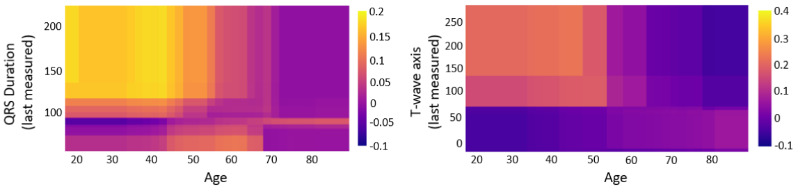
Figure 4: The EBM’s shape functions for the interaction terms between (1) age and the QRS duration last measured, and (2) age and the T-wave axis last measured.

5 Discussion

5.1 Machine learning insights

The results in Table 1 seem to suggest that state-of-the-art classification models can outperform ‘traditional’ survival models in terms of AUC when included in our pipeline, while the Brier scores are comparable. Furthermore, the EBM seems to slightly outperform XGBoost, while the EBM is an interpretable model, suggesting the EBM might be an appropriate choice for survival stacked data as well as tabular data more generally. This suggests that the pipeline encompassing (efficient) survival stacking, feature selection, and an interpretable model with interaction terms is appropriate for healthcare applications.

5.2 Clinical insights

The ControlBurn feature selection model as well as the EBM feature importances shed light onto the most important risk factors for heart failure. First, we find that age is the most important risk factor, aligning with existing clinical understanding. Our study also identifies novel risk factors for incident heart failure. We found alkaline phosphatase levels and platelet count, both markers of liver dysfunction, are also predictors of increased risk of heart failure. Other important risk factors are BMI, urea nitrogen, QRS duration, T-wave axis, and creatinine.

We also identify novel interactions between age and electrocardiographic (EKG) features (QRS duration and T-wave axis) that have not been identified in prior heart failure literature (as far as we are aware). The interactions between age and these EKG features suggest that abnormal EKG results may be predictive of increased heart failure risk when present in younger patients.

Lastly, and perhaps surprisingly, ControlBurn did not pick up gender and race as important risk factors. This is interesting because this might suggest that gender and race have limited signal for predicting heart failure after controlling for other clinical features that may be more proximal to incident heart failure.

Limitations

While the addition of subsampling helps survival stacking better scale to large data sets, there is still a significant challenge in terms of memory when building the survival stacked data set. In our heart failure experiments, our training survival stacked data set has approximately 20.7 million rows from an initial training cohort of about 290,000 patients when using $\gamma=0.01$ for subsampling. For data sets larger than ours, it is possible that the data would have trouble fitting into memory without significantly more computational resources, in which case additional methodology such as mini-batching might be helpful. Additionally, we note that our data set comes from a single healthcare system; we have added relevant data characteristics in Table 2 for reference. Our results could be more robustly tested through experiments on additional healthcare systems.

6 Conclusions

We propose a novel pipeline for interpretable survival analysis that includes efficient survival stacking, feature selection through ControlBurn, and interpretable yet accurate predictions through EBMs. We show that this pipeline outperforms survival models such as the Cox model and Random Survival Forests, while also yielding interpretable results including feature importances and shape functions describing the individual and joint contributions of features to prediction. Our pipeline validates current understanding of heart failure, while also identifying novel risk factors for incident heart failure. We hope that our pipeline is useful to the community for healthcare applications more broadly.

Appendix A Survival Analysis

Survival analysis aims to estimate the distribution of a time-to-event variable $T$ for some event of interest. In the context of healthcare, survival analysis typically involves predicting if and when a patient will develop some condition or disease. Formally, survival data for patient $i$ comes in the form $(X_{i},T_{i},\delta_{i})$, where $X_{i}$ is a vector of covariate values, $T_{i}$ is the time when the event occurs, and $\delta_{i}$ is the censoring indicator, which indicates if, at time $T_{i}$, patient $i$ develops the condition of interest or is lost to future observation without developing the condition. Survival analysis aims to estimate the probability that patient $i$ survives (that is, does not develop the condition of interest) by time $t$, $S(t\mid X_{i})=P(T_{i}>t\mid X_{i})$. Estimating $S(t\mid X_{i})$ is important for healthcare, as it can identify at-risk patients and help healthcare professionals provide appropriate treatments or risk reduction strategies.

Survival models typically aim to predict the hazard function $\lambda(t\mid X_{i})$, which represents the instantaneous risk (probability) at time $t$ given $T_{i}>t$. For example, Cox models fit a log-linear function for the hazard function:

$$\lambda(t\mid X_{i})=\lambda_{0}(t)\exp(X_{i}^{T}\beta).$$ (7)

After estimating the hazard function, the survival probability $S(t\mid X_{i})$ can be estimated by using the relationship

$$S(t\mid X_{i})=\exp(-\Lambda(t\mid X_{i})),$$ (8)

where $\Lambda(t\mid X_{i})=\int_{0}^{t}\lambda(s\mid X_{i})ds$ is the cumulative hazard function. See (Jenkins, 2005) for more details.

A.1 Survival Curves With Discrete Times

The survival probability $S(t\mid X)=P(T>t\mid X)$ represents the probability that a patient survives past time $t$, typing assuming that $T$ is continuous. However, sometimes it is reasonable to assume that $T$ is discrete, i.e. that patients can only reach the event of interest at a finite set of times. This is sometimes referred to as discrete-time modeling, see (Suresh et al., 2022).

In such cases, we can derive $S(t\mid X)$ as a function of the hazard function $\lambda$ without the integral present in Eq. (8). The result uses the following theorem:

Theorem A.1.

Let $X$ be a discrete random variable, and let $t_{1}\leq t_{2}$ be in the support of $X$. Then

$$P(X>t_{2})=P(X>t_{2}\mid X>t_{1})P(X>t_{1})$$ (9)

Proof A.2.

$$P(X>t_{2} \mid X>t_{1})P(X>t_{1})$$ (10)

$$=\frac{P(X>t_{2},X>t_{1})}{P(X>t_{1})}P(X>t_{1})$$ (11)

$$=P(X>t_{2})$$ (12)

Now, let $T$ have finite support, then by recursively applying Theorem A.1 to all times $t_{1},\ldots,t_{k}\leq t$ in the support of $T$, we have

$$S(t\mid X)=P(T>t\mid X)$$ (13)

$$=P(T>t_{1}\mid X)\prod_{i=1}^{k}P(T>t_{i+1}|T>t_{i},X)$$ (14)

Additionally, when $T$ has finite support, the hazard function can be written as

$$\lambda(t\mid X)=P(T=t\mid T\geq t,X).$$ (15)

Thus, we have

$$S(t\mid X)=P(T>t\mid X)$$ (16)

$$=P(T>t_{1}\mid X)\prod_{i=1}^{k}P(T>t_{i+1}|T>t_{i},X)$$ (17)

$$=\prod_{i=1}^{k}P(T>t_{i}|T\geq t_{i},X)$$ (18)

$$=\prod_{i=1}^{k}\Big{(}1-\lambda(t_{i}\mid X)\Big{)},$$ (19)

as in Eq. (3). For further investigation, see (Suresh et al., 2022).

Appendix B Cohort Details

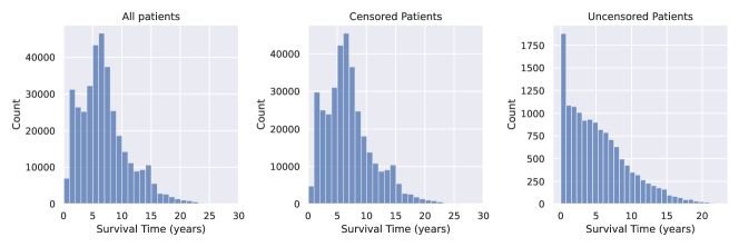
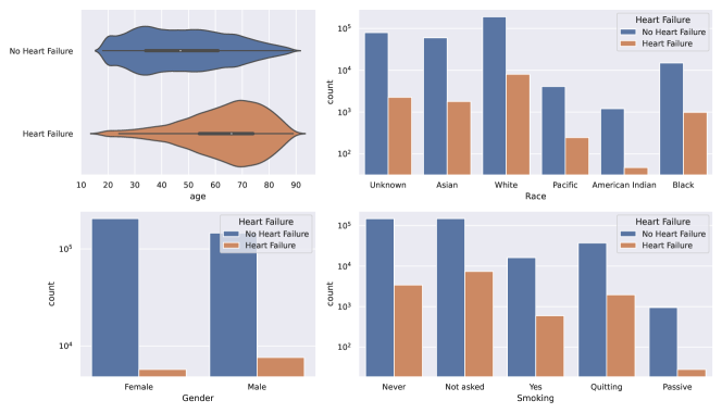
Figure 5: Additional figures to illustrate cohort characteristics. Top: distribution of survival time for patients in our cohort, for all patients, censored patients, and uncensored (heart failure) patients. Bottom: plots showing the relationship between heart failure and the demographic features in the cohort.

We evaluate our interpretable survival analysis pipeline through a large-scale study of incident heart failure risk prediction. Specifically, we gather EHR data from a large-scale hospital network (name censored for anonymity) for a total of $n=363,398$ patients and $p=1,590$ features. Data characteristics of our cohort are given in Table 2, and an additional cohort exploratory data analysis is in Appendix B.4.

Table 2: Heart Failure Cohort Statistics. More details on each individual feature is found in Table LABEL:tab:cohort_stats_all_fts.

Summary	Total Features By Type	Gender	Race	Age
$n=363398$	Measurements: 1203	Male: 42.1%	White: 54.6%	18-29: 15.8%
$p=1590$	Conditions: 115	Female: 57.9%	Asian: 17.0%	30-44: 28.5%
HF Prevalence: 3.7%	Drugs: 268		Black: 4.4%	45-59: 26.6%
	Demographics: 4		Other: 1.5%	60-74: 20.8%
			Unknown: 22.5%	$\geq 75$: 8.3%

B.1 Filtering and Censoring

We consider patients above the age of 18 with at least 3 years of continuous observation in the healthcare system. We set the index date, i.e. the prediction date, for each patient as 2 years after the start of continuous observation, and use any data prior to the index date as the raw input data. Additionally, we only consider patients with an index date before January 1, 2018 to allow for a sufficient follow-up period. Lastly, we exclude patients who developed HF prior to their index date.

For censoring, we right-censor patients at the time of death as well as at the last known encounter time if one of these occurs before a heart failure diagnosis. Additionally, since we set the index date as the earliest date with 2 years of prior observation, our cohort includes patients with long observation periods. Therefore, we also apply right-censoring at 15 years for patients that have not already been censored or had heart failure, which censors an additional 4.5% of patients in our cohort.

B.2 Data Extraction and Features

The EHR data that we use to construct our cohort is stored in the OMOP Common Data Model (CDM), an open community data standard for storing EHR data (Hripcsak et al., 2015). Thus, our data extraction pipeline is easily applicable to any EHR database stored using the OMOP CDM. Below we list the feature types that we extract, along with the OMOP CDM table that the features come from.

• Measurements: vital signs and lab measurements from the measurements table. For each measurement, we generate features for the min, max, mean, standard deviation, last observed value, and count of observed values over the patient’s historical data prior to the index date.

• Conditions: binary features indicating whether or not a patient has had the given condition at any point before the index date, coming from the condition occurrence table.

• Medications: similar to conditions, but for prescriptions and over-the-counter drugs, coming from the drug exposure table.

• Demographics: features include the patient’s age, gender, and race from the person table, and smoking history from the observation table.

Altogether, this yields 1590 features observed in the data set. These features capture current as well as historical data for patients at their index dates, which is an improvement over heart failure models that only use patient data at the index date (Khan et al., 2019; Ahmad et al., 2017).

B.3 Heart Failure Labeling

We generate survival labels $(T_{i},\delta_{i})$ for each patient $i$. The time $T_{i}$ represents the patient’s event time, which is either the time the patient gets heart failure ($\delta_{i}=1$), or the time they are lost to followup ($\delta_{i}=0$). We determine whether or not a patient got heart failure using a curated OMOP CDM concept set, which defines all concepts in the raw data associated with heart failure diagnosis. This concept set was verified by clinicians, but given the large sample size, a small mislabeling risk cannot be ruled out.

B.4 Cohort Statistics

For a list of all cohort features and their $10^{\textnormal{th}},25^{\textnormal{th}},50^{\textnormal{th}},75^{\textnormal{th}}$, and $90^{\textnormal{th}}$ percentiles, please see Table LABEL:tab:cohort_stats_all_fts. Additionally, in Figure 5, we show additional plots to visualize the distribution of survival time as well as the demographic features in the cohort.

Appendix C Additional Experiment Details

We use the following packages for our experiments:

• InterpretML: for EBM implementation (Nori et al., 2019).

• scikit-survival: for Cox models, as well as for calculating time-dependent AUC and brier metrics (Pölsterl, 2020).

• pysurvival: for Random Survival Forest implementation (Fotso et al., 2019–).

• scikit-learn: for logistic regression as well as LASSO for feature selection (Pedregosa et al., 2011).

• XGBoost: for running XGBoost (Chen and Guestrin, 2016).

Additionally, we use the following hyperparameters for our models:

• EBM: We use outer_bags=25 and inner_bags=10 to ensure robustness, and further use max_bins=64, interactions=20, max_rounds=5000 for expressivity.

• XGBoost: We use default hyperparameters.

• LogReg: The saga solver is used, motivated by the high-dimensionality of our data.

• CoxPH: we use the default hyperparameters from scikit-survival.

• RSF: we use the default hyperparameters in pysurvival: max_features=sqrt, min_node_size=10, sample_size_pct=0.63.

Appendix D Feature Selection

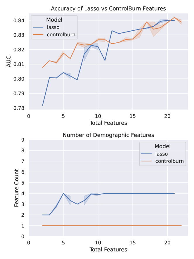
Figure 6: Comparison of linear LASSO and ControlBurn for feature selection. Each model is run for 30 regularization parameters, with each run consisting of 5 trials with different random seeds. Each trial is evaluated by running an XGBoost model on the selected features. For categorical features, if any of the one hot encoded features are selected, all are included and are collectively counted as 1 feature. The left plot shows the AUC for 5-year risk prediction for each model. The right plot shows what types of features are being selected. Errors represent standard error across trials if multiple trials result in the same number of features.

We assess the ability of ControlBurn (discussed in Section 3.3) and the linear LASSO (Tibshirani, 1996) to select useful features for predicting heart failure. Since the survival stacked data contains not only many samples but also many features, we run feature selection on a 5-year heart failure classification task as a proxy for the full survival analysis problem. We compare the performance of ControlBurn and LASSO by evaluating the performance of an XGBoost model trained using the selected features. The results as a function of the number of features selected are shown in Figure 6.

The top plot in Figure 6 demonstrates that ControlBurn selects better features than LASSO in terms of the resulting 5-year risk predictions when the number of features is roughly less than 10. When the number of features increases past 10, the methods perform similarly. The bottom plot in Figure 6 helps explain the difference between ControlBurn and LASSO in terms of what types of features are being selected. Evidently, ControlBurn selects measurement features more often, while LASSO first selects demographic features before selecting more measurement features. Since ControlBurn performs comparably to LASSO overall, and better for smaller feature sets, this suggests that demographic features such as gender and race, which the LASSO model selects, may provide no more signal than additional measurement features. One possible explanation for this behavior is that the demographic features might provide more linear signal and are thus selected by LASSO. On the other hand, the measurement features often appear to contain comparatively stronger nonlinear signal, see e.g. Figure 7, which ControlBurn tends to capture. These results demonstrate the utility of ControlBurn for selecting an appropriate subset of features for nonlinear prediction models, especially when generating small feature sets.

Appendix E Additional Experiment Results

Along with the shape functions and interaction terms shown in Figures 3 and 4, we present the most important features by global feature importance in Figure 7. Age appears to be the most important feature, while the feature importance plot also recognises other traditional risk factors as discussed in depth in Section 5.

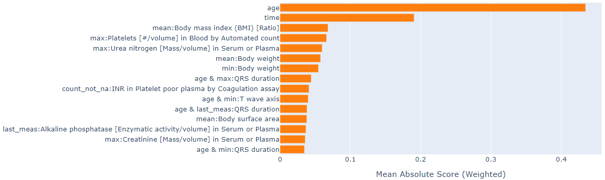
Figure 7: The EBM’s feature importances, measured through averaging the feature’s absolute contributions to risk over all samples. Age is a significantly better predictor than the other features. Additionally, most interaction terms include age, suggesting age is also an important feature in combination with other features after accounting for its individual contribution.

Table 3: This table shows the $10^{\textnormal{th}},25^{\textnormal{th}},50^{\textnormal{th}},75^{\textnormal{th}}$, and $90^{\textnormal{th}}$ percentiles of all features picked up by at least one feature selection method.

Percentile	10${}^{\textnormal{th}}$	25${}^{\textnormal{th}}$	50${}^{\textnormal{th}}$	75${}^{\textnormal{th}}$	90${}^{\textnormal{th}}$
last_meas:Pulse rate	60.00	66.00	75.00	84.00	94.00
mean:Prothrombin time (PT)	11.67	12.60	13.60	14.70	17.08
min:Venous oxygen saturation measurement	45.00	63.00	73.00	84.10	93.20
count_not_na:Aspartate aminotransferase measurement	1.00	1.00	1.00	1.00	3.00
mean:Urea nitrogen [Mass/volume] in Serum or Plasma	8.50	11.00	14.00	17.00	22.00
min:Diastolic blood pressure	57.00	63.00	70.00	78.00	84.00
mean:Thyroid stimulating hormone measurement	0.72	1.10	1.65	2.43	3.42
cond:Gastroesophageal reflux disease	0.00	0.00	0.00	0.00	0.00
max:Cholesterol.total/Cholesterol in HDL [Mass Ratio] in Serum or Plasma	3.20	51.00	115.00	150.00	183.00
mean:Oxygen [Partial pressure] in Arterial blood	82.12	119.05	177.92	231.00	283.36
mean:Erythrocyte distribution width [Ratio] by Automated count	12.50	13.00	13.60	14.50	16.00
mean:Chloride [Moles/volume] in Serum or Plasma	99.50	101.43	103.00	105.00	107.00
max:Triglyceride [Moles/volume] in Serum or Plasma	50.00	70.00	104.00	160.00	241.00
max:Glomerular filtration rate/1.73 sq M.predicted	57.00	60.00	66.00	102.00	120.00
in Serum, Plasma or Blood by Creatinine-based formula (MDRD)
count_not_na:Chloride [Moles/volume] in Serum or Plasma	1.00	1.00	2.00	4.00	11.00
max:Base excess measurement	0.30	0.80	1.90	3.70	6.20
min:T wave axis	-10.00	10.00	30.00	48.00	68.00
last_meas:Triglyceride [Moles/volume] in Serum or Plasma	48.00	66.00	97.00	146.00	215.00
count_not_na:Thyroid stimulating hormone measurement	1.00	1.00	1.00	1.00	1.00
mean:High density lipoprotein measurement	36.00	43.00	53.00	66.00	79.00
mean:Basophils/100 leukocytes in Blood by Automated count	0.10	0.27	0.40	0.60	0.90
last_meas:Creatine kinase.MB [Mass/volume] in Blood	0.50	0.71	1.58	3.19	10.50
last_meas:Glucose [Mass/volume] in Serum or Plasma	84.00	91.00	100.00	116.00	145.00
mean:Hemoglobin A1c/Hemoglobin.total in Blood	5.00	5.30	5.70	6.30	7.67
last_meas:Q-T interval corrected	391.00	404.00	419.00	436.00	455.00
min:Prothrombin time (PT)	11.30	12.20	13.10	13.90	14.90
mean:Carbon dioxide, total [Moles/volume] in Serum or Plasma	23.25	25.00	27.00	28.50	30.00
min:Body weight	1888.00	2160.00	2560.00	3040.00	3555.20
last_meas:Left ventricular Ejection fraction	53.20	57.70	62.10	66.30	70.20
min:Body surface area	1.54	1.67	1.84	2.04	2.22
max:Left ventricular Ejection fraction	54.20	58.00	62.70	67.00	70.70
max:Platelets [#/volume] in Blood by Automated count	173.00	208.00	252.00	309.00	385.00
min:Urea nitrogen [Mass/volume] in Serum or Plasma	6.00	9.00	12.00	16.00	20.00
mean:Creatinine [Mass/volume] in Serum or Plasma	0.65	0.76	0.90	1.07	1.26
std:P wave axis	2.12	4.60	9.37	17.79	31.11
count_not_na:Venous oxygen saturation measurement	1.00	1.00	1.00	2.00	5.00
std:Sodium [Moles/volume] in Serum or Plasma	0.58	1.15	2.00	2.83	3.67
min:Erythrocyte distribution width [Ratio] by Automated count	12.30	12.70	13.30	14.00	15.00
min:Chloride measurement, blood	101.00	105.00	108.00	111.00	113.00
max:Cholesterol in LDL [Mass/volume] in Serum or Plasma by Direct assay	72.00	91.00	114.00	139.00	165.00
max:Glucose [Mass/volume] in Serum or Plasma	87.00	95.00	110.00	146.00	200.00
last_meas:Lymphocytes/100 leukocytes in Blood by Automated count	9.10	15.70	24.10	31.80	38.30
std:Q-T interval corrected	0.00	0.00	0.00	6.59	16.74
mean:P-R Interval	136.00	148.00	162.00	180.00	198.00
count_not_na:INR in Platelet poor plasma by Coagulation assay	1.00	1.00	2.00	4.00	9.00
mean:Systolic blood pressure	106.00	113.50	123.00	133.33	144.33
mean:Body height	61.00	63.00	66.00	69.00	72.00
last_meas:Venous oxygen saturation measurement	51.00	67.22	76.00	86.40	94.30
min:Cholesterol [Mass/volume] in Serum or Plasma	130.00	152.00	178.00	204.00	231.00
max:QRS duration	78.00	84.00	90.00	100.00	112.00
std:Glucose [Mass/volume] in Serum or Plasma	2.12	7.07	16.26	28.20	46.05
drug:aspirin 325 MG Oral Tablet	0.00	0.00	0.00	0.00	0.00
mean:Globulin [Mass/volume] in Serum	2.50	2.90	3.40	3.80	4.20
mean:Glucose [Mass/volume] in Serum or Plasma	86.00	93.00	103.50	121.00	147.00
std:Pulse rate	2.83	5.29	8.12	11.31	14.96
max:Globulin [Mass/volume] in Serum	2.60	3.00	3.50	4.00	4.50
max:Hemoglobin [Mass/volume] in Blood	11.60	12.70	13.70	14.80	15.70
last_meas:Cholesterol non HDL [Mass/volume] in Serum or Plasma	79.00	96.00	121.00	149.00	177.00
min:Oxygen saturation measurement	28.00	42.00	61.00	79.00	91.00
max:Lactate [Mass/volume] in Blood	0.69	0.96	1.42	2.18	3.28
min:R-R interval by EKG	556.00	667.00	800.00	923.00	1053.00
last_meas:Thyroid stimulating hormone measurement	0.71	1.10	1.64	2.41	3.40
min:Vancomycin [Mass/volume] in Serum or Plasma –trough	3.10	5.40	8.30	12.00	16.48
std:Oxygen [Partial pressure] in Venous blood	0.21	2.48	7.07	14.62	28.24
max:Creatinine measurement	0.68	0.80	1.00	2.98	2100.00
max:Monocytes [#/volume] in Blood by Manual count	0.20	0.40	0.70	1.30	2.17
max:Body height	61.22	63.00	66.00	69.02	72.00
last_meas:INR in Platelet poor plasma by Coagulation assay	1.00	1.00	1.10	1.20	1.40
cond:Atrial fibrillation	0.00	0.00	0.00	0.00	0.00
mean:Anion gap in Serum or Plasma	5.00	6.22	7.73	9.00	11.00
count_not_na:Low density lipoprotein measurement	1.00	1.00	1.00	1.00	1.00
mean:Diastolic blood pressure	63.50	69.00	75.00	81.00	87.00
last_meas:Prothrombin time (PT)	11.60	12.50	13.50	14.50	16.70
last_meas:Creatinine measurement	0.67	0.80	1.00	1.92	1980.00
max:Cholesterol [Mass/volume] in Serum or Plasma	138.00	160.00	186.00	215.00	244.00
std:Urea nitrogen [Mass/volume] in Serum or Plasma	0.58	1.41	2.79	4.24	6.45
min:Creatinine [Mass/volume] in Serum or Plasma	0.60	0.70	0.82	1.00	1.20
mean:Body weight	1929.47	2208.00	2616.00	3100.55	3625.07
min:Creatinine measurement	0.66	0.80	1.00	1.85	1904.90
max:Urea nitrogen [Mass/volume] in Serum or Plasma	9.00	12.00	15.00	20.00	27.00
min:Creatine kinase [Enzymatic activity/volume] in Serum or Plasma	31.00	54.00	93.00	183.00	477.00
count_not_na:Glucose measurement, blood	1.00	1.00	1.00	3.00	7.00
max:T wave axis	4.00	20.00	39.00	58.00	86.00
mean:Calcium [Mass/volume] in Serum or Plasma	8.28	8.65	9.00	9.35	9.60
last_meas:Leukocytes [#/volume] in Specimen by Automated count	4.50	5.60	7.00	9.00	11.60
mean:Venous oxygen saturation measurement	54.15	68.00	76.42	85.60	93.50
min:Body height	61.00	63.00	66.00	69.00	72.00
drug:hydrochlorothiazide 25 MG Oral Tablet	0.00	0.00	0.00	0.00	0.00
min:Pulse rate	55.00	61.00	69.00	78.00	88.00
std:QRS axis	2.08	4.24	8.33	14.59	24.75
min:Left ventricular Ejection fraction	52.24	57.10	61.70	66.00	70.00
count_not_na:Calcium [Mass/volume] in Serum or Plasma	1.00	1.00	2.00	4.00	11.00
max:Systolic blood pressure	109.00	118.00	129.00	142.00	156.00
mean:Measurement of venous partial pressure of carbon dioxide	34.05	38.60	43.10	47.40	51.50
min:Hemoglobin level estimation	10.00	11.80	13.10	14.30	15.30
last_meas:QRS duration	76.00	82.00	90.00	98.00	110.00
count_not_na:Urea nitrogen [Mass/volume] in Serum or Plasma	1.00	1.00	2.00	4.00	11.00
min:Leukocytes [#/volume] in Blood by Automated count	3.78	4.35	4.97	7.30	10.60
last_meas:Alkaline phosphatase [Enzymatic activity/volume]	50.00	61.00	78.00	99.00	127.00
in Serum or Plasma
min:P wave axis	0.00	23.00	43.00	59.00	70.00
last_meas:Platelets [#/volume] in Blood by Automated count	153.00	191.00	233.00	281.00	338.00
mean:Leukocytes [#/volume] in Blood by Automated count	4.00	4.46	5.12	8.10	11.50
max:Monocytes/100 leukocytes in Blood by Automated count	5.10	6.50	8.10	10.40	13.40
max:Thyroid stimulating hormone measurement	0.73	1.12	1.67	2.46	3.50
max:Lymphocytes [#/volume] in Blood by Automated count	1.00	1.39	1.85	2.42	3.22
min:Alkaline phosphatase [Enzymatic activity/volume] in Serum or Plasma	46.00	57.00	72.00	90.00	113.00
last_meas:Erythrocyte distribution width [Ratio] by Automated count	12.50	13.00	13.60	14.40	15.90
mean:Body mass index (BMI) [Ratio]	20.76	23.02	26.11	30.12	35.01
count_not_na:P wave axis	1.00	1.00	1.00	2.00	4.00
mean:Pulse rate	61.00	67.80	75.00	83.33	91.80
count_not_na:Hemoglobin level estimation	1.00	1.00	1.00	1.00	4.00
mean:Fractional oxyhemoglobin in Arterial blood	94.30	96.25	97.30	97.90	98.40
mean:Lymphocytes/100 leukocytes in Blood by Automated count	9.78	15.40	23.20	30.90	37.30
age	26.00	34.00	48.00	62.00	73.00
max:Body surface area	1.57	1.70	1.88	2.08	2.27
mean:QRS duration	77.89	82.67	90.00	98.00	109.00
mean:T wave axis	1.00	16.00	35.00	52.00	73.50
mean:MCHC [Mass/volume] by Automated count	32.70	33.30	33.90	34.40	34.80
min:INR in Platelet poor plasma by Coagulation assay	1.00	1.00	1.10	1.10	1.20
std:Bilirubin.direct [Mass/volume] in Serum or Plasma	0.00	0.00	0.05	0.14	0.71
mean:Cholesterol [Mass/volume] in Serum or Plasma	135.93	157.00	182.00	209.00	235.00
last_meas:Body weight	1923.20	2208.00	2620.80	3104.00	3632.00
mean:Body surface area	1.56	1.68	1.86	2.06	2.25
max:MCHC [Mass/volume] by Automated count	32.90	33.60	34.20	34.80	35.30
min:Sodium [Moles/volume] in Serum or Plasma	132.00	135.00	137.00	139.00	141.00
min:Aspartate aminotransferase [Enzymatic activity/volume] in Serum or Plasma	13.00	17.00	21.00	27.00	37.00
last_meas:Systolic blood pressure	104.00	112.00	122.00	134.00	147.00
max:Q-T interval corrected	395.00	408.00	423.00	442.00	463.20
min:MCHC [Mass/volume] by Automated count	32.20	32.90	33.60	34.20	34.60
max:Basophils [#/volume] in Blood by Automated count	0.01	0.02	0.04	0.06	0.10
last_meas:QRS axis	-28.00	-2.00	27.00	55.00	74.00
max:Myoglobin [Presence] in Serum or Plasma	25.00	32.00	46.00	82.00	194.00
last_meas:Anion gap in Serum or Plasma	5.00	6.00	8.00	9.00	11.00
mean:Chloride measurement, blood	104.00	106.73	109.75	112.33	114.67
last_meas:Body temperature	97.20	97.60	98.00	98.40	98.70
std:Prothrombin time (PT)	0.14	0.41	0.80	1.68	4.62
max:Thyroxine (T4) free [Mass/volume] in Serum or Plasma	0.90	1.00	1.20	1.37	1.60
last_meas:T wave axis	-1.00	16.00	35.00	53.00	74.00
std:Cholesterol.total/Cholesterol in HDL [Mass Ratio] in Serum or Plasma	43.99	61.17	79.08	97.72	116.04
min:QRS duration	76.00	82.00	88.00	96.00	106.00
min:Chloride [Moles/volume] in Serum or Plasma	97.00	100.00	102.00	104.00	106.00
mean:Creatinine measurement	0.67	0.80	1.00	2.80	1980.00
min:Thyrotropin [Units/volume] in Serum or Plasma	0.48	0.89	1.39	2.10	3.06
drug:1 ML hydromorphone hydrochloride 2 MG/ML Injection	0.00	0.00	0.00	0.00	0.00
max:Body weight	1964.74	2243.40	2663.16	3160.51	3700.20
mean:Q-T interval corrected	392.00	405.00	419.50	436.00	453.50
min:aPTT in Platelet poor plasma by Coagulation assay	25.10	27.20	29.80	32.80	36.80
max:Creatinine [Mass/volume] in Serum or Plasma	0.70	0.80	0.97	1.13	1.40
mean:Glomerular filtration rate/1.73 sq M.predicted	55.00	60.00	60.00	60.00	60.00
[Volume Rate/Area] in Serum, Plasma or Blood by CKD-EPI
min:Hematocrit [Volume Fraction] of Blood	30.00	35.00	38.70	42.00	45.00
last_meas:Globulin [Mass/volume] in Serum	2.50	2.90	3.40	3.80	4.20
min:Body temperature	96.80	97.30	97.70	98.10	98.50
last_meas:Creatinine [Mass/volume] in Serum or Plasma	0.64	0.75	0.90	1.10	1.30
min:Eosinophils [#/volume] in Blood by Automated count	0.00	0.02	0.08	0.16	0.30
max:Body mass index (BMI) [Ratio]	21.10	23.44	26.63	30.78	35.87
drug:fentanyl 0.05 MG/ML Injection	0.00	0.00	0.00	0.00	1.00
drug:2 ML ondansetron 2 MG/ML Injection	0.00	0.00	0.00	0.00	1.00
last_meas:Urea nitrogen [Mass/volume] in Serum or Plasma	8.00	11.00	14.00	17.00	22.00
min:Eosinophils/100 leukocytes in Blood by Automated count	0.00	0.20	1.00	2.10	3.70

References

- Agarwal et al. (2021) Rishabh Agarwal, Levi Melnick, Nicholas Frosst, Xuezhou Zhang, Ben Lengerich, Rich Caruana, and Geoffrey E Hinton. Neural additive models: Interpretable machine learning with neural nets. Advances in Neural Information Processing Systems, 34:4699–4711, 2021.
- Ahmad et al. (2017) Tanvir Ahmad, Assia Munir, Sajjad Haider Bhatti, Muhammad Aftab, and Muhammad Ali Raza. Survival analysis of heart failure patients: A case study. PloS one, 12(7):e0181001, 2017.
- Alvarez-Melis and Jaakkola (2018) David Alvarez-Melis and Tommi S Jaakkola. On the robustness of interpretability methods. arXiv preprint arXiv:1806.08049, 2018.
- Andersen and Pohar Perme (2010) Per Kragh Andersen and Maja Pohar Perme. Pseudo-observations in survival analysis. Statistical methods in medical research, 19(1):71–99, 2010.
- Binder et al. (2014) Nadine Binder, Thomas A Gerds, and Per Kragh Andersen. Pseudo-observations for competing risks with covariate dependent censoring. Lifetime data analysis, 20:303–315, 2014.
- Bosschieter et al. (2022) Tomas M Bosschieter, Zifei Xu, Hui Lan, Benjamin J Lengerich, Harsha Nori, Kristin Sitcov, Vivienne Souter, and Rich Caruana. Using interpretable machine learning to predict maternal and fetal outcomes. arXiv preprint arXiv:2207.05322, 2022.
- CDC (2023) CDC. Heart failure, 2023. URL https://www.cdc.gov/heartdisease/heart_failure.htm.
- Chen and Guestrin (2016) Tianqi Chen and Carlos Guestrin. Xgboost: A scalable tree boosting system. In Proceedings of the 22nd acm sigkdd international conference on knowledge discovery and data mining, pages 785–794, 2016.
- Chicco and Jurman (2020) Davide Chicco and Giuseppe Jurman. Machine learning can predict survival of patients with heart failure from serum creatinine and ejection fraction alone. BMC medical informatics and decision making, 20(1):1–16, 2020.
- Cox (1972) David R Cox. Regression models and life-tables. Journal of the Royal Statistical Society: Series B (Methodological), 34(2):187–202, 1972.
- Craig et al. (2021) Erin Craig, Chenyang Zhong, and Robert Tibshirani. Survival stacking: casting survival analysis as a classification problem. arXiv preprint arXiv:2107.13480, 2021.
- Fahmy et al. (2021) Ahmed S Fahmy, Ethan J Rowin, Warren J Manning, Martin S Maron, and Reza Nezafat. Machine learning for predicting heart failure progression in hypertrophic cardiomyopathy. Frontiers in cardiovascular medicine, 8:647857, 2021.
- Feng and Zhao (2021) Dai Feng and Lili Zhao. Bdnnsurv: Bayesian deep neural networks for survival analysis using pseudo values. arXiv preprint arXiv:2101.03170, 2021.
- Fotso et al. (2019–) Stephane Fotso et al. PySurvival: Open source package for survival analysis modeling, 2019–. URL https://www.pysurvival.io/.
- Giunchiglia et al. (2018) Eleonora Giunchiglia, Anton Nemchenko, and Mihaela van der Schaar. Rnn-surv: A deep recurrent model for survival analysis. In Artificial Neural Networks and Machine Learning–ICANN 2018: 27th International Conference on Artificial Neural Networks, Rhodes, Greece, October 4-7, 2018, Proceedings, Part III 27, pages 23–32. Springer, 2018.
- Hastie and Tibshirani (1995) Trevor Hastie and Robert Tibshirani. Generalized additive models for medical research. Statistical methods in medical research, 4(3):187–196, 1995.
- Hastie (2017) Trevor J Hastie. Generalized additive models. In Statistical models in S, pages 249–307. Routledge, 2017.
- Hripcsak et al. (2015) George Hripcsak, Jon D Duke, Nigam H Shah, Christian G Reich, Vojtech Huser, Martijn J Schuemie, Marc A Suchard, Rae Woong Park, Ian Chi Kei Wong, Peter R Rijnbeek, et al. Observational health data sciences and informatics (ohdsi): opportunities for observational researchers. In MEDINFO 2015: eHealth-enabled Health, pages 574–578. IOS Press, 2015.
- Ishwaran et al. (2008) Hemant Ishwaran, Udaya B Kogalur, Eugene H Blackstone, and Michael S Lauer. Random survival forests. 2008.
- Jenkins (2005) Stephen P Jenkins. Survival analysis. Unpublished manuscript, Institute for Social and Economic Research, University of Essex, Colchester, UK, 42:54–56, 2005.
- Kamath and Liu (2021) Uday Kamath and John Liu. Explainable artificial intelligence: An introduction to interpretable machine learning. Springer, 2021.
- Katzman et al. (2018) Jared L Katzman, Uri Shaham, Alexander Cloninger, Jonathan Bates, Tingting Jiang, and Yuval Kluger. Deepsurv: personalized treatment recommender system using a cox proportional hazards deep neural network. BMC medical research methodology, 18(1):1–12, 2018.
- Khan et al. (2019) Sadiya S Khan, Hongyan Ning, Sanjiv J Shah, Clyde W Yancy, Mercedes Carnethon, Jarett D Berry, Robert J Mentz, Emily O’Brien, Adolfo Correa, Navin Suthahar, et al. 10-year risk equations for incident heart failure in the general population. Journal of the American College of Cardiology, 73(19):2388–2397, 2019.
- Kumar et al. (2020) I Elizabeth Kumar, Suresh Venkatasubramanian, Carlos Scheidegger, and Sorelle Friedler. Problems with shapley-value-based explanations as feature importance measures. In International Conference on Machine Learning, pages 5491–5500. PMLR, 2020.
- Lee et al. (2018) Changhee Lee, William Zame, Jinsung Yoon, and Mihaela Van Der Schaar. Deephit: A deep learning approach to survival analysis with competing risks. In Proceedings of the AAAI conference on artificial intelligence, volume 32, 2018.
- Lengerich et al. (2020) Benjamin Lengerich, Sarah Tan, Chun-Hao Chang, Giles Hooker, and Rich Caruana. Purifying interaction effects with the functional anova: An efficient algorithm for recovering identifiable additive models. In International Conference on Artificial Intelligence and Statistics, pages 2402–2412. PMLR, 2020.
- Lengerich et al. (2022) Benjamin J Lengerich, Rich Caruana, Mark E Nunnally, and Manolis Kellis. Death by round numbers and sharp thresholds: how to avoid dangerous ai ehr recommendations. medRxiv, 2022.
- Liu et al. (2021) Brian Liu, Miaolan Xie, and Madeleine Udell. ControlBurn: Feature selection by sparse forests. In Proceedings of the 27th ACM SIGKDD Conference on Knowledge Discovery & Data Mining, pages 1045–1054, 2021.
- Liu et al. (2022) Brian Liu, Miaolan Xie, Haoyue Yang, and Madeleine Udell. Controlburn: Nonlinear feature selection with sparse tree ensembles. arXiv preprint arXiv:2207.03935, 2022.
- Lou et al. (2012) Yin Lou, Rich Caruana, and Johannes Gehrke. Intelligible models for classification and regression. In Proceedings of the 18th ACM SIGKDD international conference on Knowledge discovery and data mining, pages 150–158, 2012.
- Lou et al. (2013) Yin Lou, Rich Caruana, Johannes Gehrke, and Giles Hooker. Accurate intelligible models with pairwise interactions. In Proceedings of the 19th ACM SIGKDD international conference on Knowledge discovery and data mining, pages 623–631. ACM, 2013.
- Lundberg and Lee (2017) Scott M Lundberg and Su-In Lee. A unified approach to interpreting model predictions. Advances in neural information processing systems, 30, 2017.
- Newaz et al. (2021) Asif Newaz, Nadim Ahmed, and Farhan Shahriyar Haq. Survival prediction of heart failure patients using machine learning techniques. Informatics in Medicine Unlocked, 26:100772, 2021.
- Nori et al. (2019) Harsha Nori, Samuel Jenkins, Paul Koch, and Rich Caruana. Interpretml: A unified framework for machine learning interpretability. arXiv preprint arXiv:1909.09223, 2019.
- Nori et al. (2021) Harsha Nori, Rich Caruana, Zhiqi Bu, Judy Hanwen Shen, and Janardhan Kulkarni. Accuracy, interpretability, and differential privacy via explainable boosting. In International Conference on Machine Learning, pages 8227–8237. PMLR, 2021.
- Panahiazar et al. (2015) Maryam Panahiazar, Vahid Taslimitehrani, Naveen Pereira, and Jyotishman Pathak. Using ehrs and machine learning for heart failure survival analysis. Studies in health technology and informatics, 216:40, 2015.
- Pedregosa et al. (2011) Fabian Pedregosa, Gaël Varoquaux, Alexandre Gramfort, Vincent Michel, Bertrand Thirion, Olivier Grisel, Mathieu Blondel, Peter Prettenhofer, Ron Weiss, Vincent Dubourg, et al. Scikit-learn: Machine learning in python. the Journal of machine Learning research, 12:2825–2830, 2011.
- Pölsterl (2020) Sebastian Pölsterl. scikit-survival: A library for time-to-event analysis built on top of scikit-learn. The Journal of Machine Learning Research, 21(1):8747–8752, 2020.
- Qu et al. (2022) Yanji Qu, Xinlei Deng, Shao Lin, Fengzhen Han, Howard H Chang, Yanqiu Ou, Zhiqiang Nie, Jinzhuang Mai, Ximeng Wang, Xiangmin Gao, et al. Using innovative machine learning methods to screen and identify predictors of congenital heart diseases. Frontiers in Cardiovascular Medicine, 8:2087, 2022.
- Rahman and Purushotham (2021) Md Mahmudur Rahman and Sanjay Purushotham. Pseudonam: A pseudo value based interpretable neural additive model for survival analysis. UMBC Student Collection, 2021.
- Rahman and Purushotham (2022a) Md Mahmudur Rahman and Sanjay Purushotham. Fair and interpretable models for survival analysis. In Proceedings of the 28th ACM SIGKDD Conference on Knowledge Discovery and Data Mining, pages 1452–1462, 2022a.
- Rahman and Purushotham (2022b) Md Mahmudur Rahman and Sanjay Purushotham. Pseudo value-based deep neural networks for multi-state survival analysis. arXiv preprint arXiv:2207.05291, 2022b.
- Rahman et al. (2021) Md Mahmudur Rahman, Koji Matsuo, Shinya Matsuzaki, and Sanjay Purushotham. Deeppseudo: Pseudo value based deep learning models for competing risk analysis. In Proceedings of the AAAI Conference on Artificial Intelligence, volume 35, pages 479–487, 2021.
- Rahnama and Boström (2019) Amir Hossein Akhavan Rahnama and Henrik Boström. A study of data and label shift in the lime framework. arXiv preprint arXiv:1910.14421, 2019.
- Ribeiro et al. (2016) Marco Tulio Ribeiro, Sameer Singh, and Carlos Guestrin. Model-agnostic interpretability of machine learning. arXiv preprint arXiv:1606.05386, 2016.
- Ridgeway (1999) Greg Ridgeway. The state of boosting. Computing science and statistics, pages 172–181, 1999.
- Sarica et al. (2021) Alessia Sarica, Andrea Quattrone, and Aldo Quattrone. Explainable boosting machine for predicting alzheimer’s disease from mri hippocampal subfields. In Brain Informatics: 14th International Conference, BI 2021, Virtual Event, September 17–19, 2021, Proceedings 14, pages 341–350. Springer, 2021.
- Suresh et al. (2022) Krithika Suresh, Cameron Severn, and Debashis Ghosh. Survival prediction models: an introduction to discrete-time modeling. BMC medical research methodology, 22(1):207, 2022.
- Tibshirani (1996) Robert Tibshirani. Regression shrinkage and selection via the lasso. Journal of the Royal Statistical Society: Series B (Methodological), 58(1):267–288, 1996.
- Tsao et al. (2022) Connie W Tsao, Aaron W Aday, Zaid I Almarzooq, Alvaro Alonso, Andrea Z Beaton, Marcio S Bittencourt, Amelia K Boehme, Alfred E Buxton, April P Carson, Yvonne Commodore-Mensah, et al. Heart disease and stroke statistics—2022 update: a report from the american heart association. Circulation, 145(8):e153–e639, 2022.
- Utkin et al. (2022) Lev V Utkin, Egor D Satyukov, and Andrei V Konstantinov. Survnam: The machine learning survival model explanation. Neural Networks, 147:81–102, 2022.
- Van Belle et al. (2007) Vanya Van Belle, Kristiaan Pelckmans, Johan Suykens, and Sabine Van Huffel. Support vector machines for survival analysis. In Proc. of the Third International Conference on Computational Intelligence in Medicine and Healthcare (CIMED2007), 2007.
- Van den Broeck et al. (2022) Guy Van den Broeck, Anton Lykov, Maximilian Schleich, and Dan Suciu. On the tractability of shap explanations. Journal of Artificial Intelligence Research, 74:851–886, 2022.
- Zhao and Feng (2019) Lili Zhao and Dai Feng. Dnnsurv: Deep neural networks for survival analysis using pseudo values. arXiv preprint arXiv:1908.02337, 2019.