On a model of online analog computation in the cell with absolute functional robustness: algebraic characterization, function compiler and error control
Abstract
The Turing completeness of continuous Chemical Reaction Networks (CRNs) states that any computable real function can be computed by a continuous CRN on a finite set of molecular species, possibly restricted to elementary reactions, i.e. with at most two reactants and mass action law kinetics. In this paper, we introduce a more stringent notion of robust online analog computation, and Absolute Functional Robustness (AFR), for the CRNs that stabilize the concentration values of some output species to the result of one function of the input species concentrations, in a perfectly robust manner with respect to perturbations of both intermediate and output species. We prove that the set of real functions stabilized by a CRN with mass action law kinetics is precisely the set of real algebraic functions. Based on this result, we present a compiler which takes as input any algebraic function (defined by one polynomial and one point for selecting one branch of the algebraic curve defined by the polynomial) and generates an abstract CRN to stabilize it. Furthermore, we provide error bounds to estimate and control the error of an unperturbed system, under the assumption that the environment inputs are driven by -Lipschitz functions.
keywords:
Analog computation, online computation, robustness, stabilization, algebraic functions, chemical reaction networks.1 Introduction
1.1 Background
Chemical Reaction Networks (CRNs) are a standard formalism used in chemistry and biology to model complex molecular interaction systems at various levels of abstraction. In the perspective of systems biology, they are a central tool to analyze the high-level functions of the cell in terms of their low-level molecular interactions. In that perspective, the Systems Biology Markup Language (SBML) [23] is a common format to exchange CRN models and build CRN model repositories, such as Biomodels.net [5] which contains thousands of CRN models of a large variety of cell biochemical processes. In the perspective of synthetic biology, they constitute a target programming language to implement in chemistry new functions either in vitro, e.g. using DNA polymers [26], or in living cells using plasmids [10] or in artificial vesicles using proteins [8].
The mathematical theory of CRNs was introduced in the late 70’s, on the one hand, by Feinberg in [15], by focusing on robust perfect adaptation (RPA) properties, Absolute Concentration Robustness (ACR) [28] and multi-stability analyses [9]; and on the other hand, by Érdi and Tóth by characterizing the set of Polynomial Ordinary Differential Equation systems (PODEs) that can be defined by CRNs with mass action law kinetics, using dual-rail encoding for negative variables [17, 11, 25, 12].
More recently, a computational theory of CRNs was investigated by formally relating their Boolean, discrete, stochastic and differential semantics in the framework of abstract interpretation [14], and by studying the computational power of CRNs under those different interpretations [7, 6, 12].
In particular, under the continuous semantics of CRNs interpreted by ODEs, the Turing-completeness result established in [12] states that any computable real function, i.e. computable by a Turing machine with an arbitrary precision given in input, can be computed by a continuous CRN on a finite set of molecular species, using elementary reactions with at most two reactants and mass action law kinetics. This result uses the following notion of analog computation of a non-negative real function computed by a CRN, where the result is given by the concentration of one species, , and the error is controlled by the concentration of one second species, :
Definition 1
[12] A function is CRN-computable if there exist a CRN over some molecular species , and a polynomial defining their initial concentration values, such that for all there exists some (necessarily unique) function such that and for all :
, is decreasing and .
From the theoretical point of view of computability, the control of the error which is explicitly represented in the above definition by the auxiliary variable , is necessary to decide when the result is ready for a requested precision, and to mathematically define the function computed by a CRN, if any.
From a practical point of view however, precision is of course an irrelevant issue since chemical reactions are stochastic in nature and a more important criterion than the precision of the result is the stability of the result and its robustness with respect to molecular concentration perturbations. With this provision to omit error control, the Turing-completeness result of continuous CRNs was immediately used in [12] to design a compilation pipeline to implement any mathematical elementary function in abstract chemistry. This compiler, implemented in our CRN modeling, analysis and synthesis software Biocham111https://lifeware.inria.fr/biocham4/ [2], generates a CRN over a finite set of abstract molecular species, through several symbolic computation steps, mainly composed of polynomialization [20], quadratization [19] and lazy dual-rail encoding of negative variables. A similar approach is undertaken in the CRN system [29], also related to [3].
It is worth remarking that in the definition above, and in our implementation in Biocham, the input is defined by the initial concentration of the input species which can be consumed by the synthesized CRN to compute the result. This marks a fundamental difference with many natural CRNs which perform a kind of online computation by adapting the response to the time evolution of the input. This is the case for instance of the ubiquitous MAPK signaling network which computes an input/output function well approximated by a Hill function of order 4.9 [22], while our synthesized CRNs to compute the same function consume their input and do not correctly adapt to change of the input value during computation [20].
1.2 Contributions
In this paper222This paper is an extended version of a previous communication at CMSB 2022 published in [18]. The main new results added to the conference proceedings are the introduction of the notion of Absolute Functional Robustness (AFR) and the mathematical analysis of the approximation error done in this new computation model by stabilization. The latter is reported in a new section of the paper devoted to error control. The computational results presented here have been obtained with a Biocham notebook available in different formats at https://lifeware.inria.fr/wiki/Main/Software#CMSB22., we introduce a new notion of online computation for continuous CRNs, by opposition to our previous static notion of computation of the result of a function for any initially given input [12]. We thus study open CRNs with species partitioned into input, intermediate and output species. The input species are supposed to be driven by the environment while the intermediate and output species are governed by the reactions of the CRN. We are interested to understand what relation can be imposed between the input and output species. Our main theorem shows that the set of input/output functions stabilized online by a CRN with mass action law kinetics, is precisely the set of real algebraic functions.
Example 2
We can illustrate this result with a simple example. Let us consider a cell that produces a receptor, , which is transformed in an active form, , when bound to an external ligand , and which stays active even after unbinding:
| (1) |
The differential semantics with mass action law of unitary rate constant is the Polynomial Ordinary Differential Equation (PODE):
| (2) |
where here and thereafter, denotes the natural multiplication. At steady state, all the derivatives are null and by eliminating , we immediately obtain the polynomial equation: . Thinking of this simple CRN as a kind of signal processing with the ligand as input and the active receptor as output, it is thus possible to find a polynomial relation between the input and the output. In this case, this relation entirely defines the function computed by the CRN:
For a given concentration of ligand, this is the only stable state of the system, independently of the initial concentrations of or . This is why we say that the CRN stabilizes the function .
Such functions, for which there exists a polynomial relation between the inputs and output, are called algebraic functions in mathematics. We show here that they characterize the set of input/output functions stabilized by CRNs with mass action law kinetics.
Furthermore, our constructive proof provides a compilation algorithm to generate a stabilizing CRN for any real algebraic curve, i.e. any curve defined by the zeros of some polynomial. We present the main symbolic transformations steps of this new compiler implemented in Biocham, and its main differences with the previous compilation scheme, in particular concerning the quadratization problem to solve [19, 20].
Then in the last Sec. 6, we provide error bounds to estimate and control the error of an unperturbed system when we suppose that the rate of change of the input functions are bounded, that is, the concentrations of the input species cannot change arbitrarily fast. Mathematically, we will provide error bounds for -Lipschitz environement input functions.
1.3 Related works
The computational framework adopted in this article is a clarification and refinement of the one already envisioned by the first author in [21]. The purpose of this previous work was to evolve a biochemically plausible CRN capable of stabilizing the logarithm of its input. Since the logarithm is not an algebraic function, we now know that the result was bound to be an approximation, which was not known at that time.
Our work may also be related to the notion of Absolute Concentration Robustness (ACR) developed by Feinberg [28]. A CRN species is said to display ACR if it has the same concentration on every stable point of the system. More generally, we introduce here the notion of Absolute Functional Robustness (AFR) for CRNs in which one output species stabilizes a function of CRN inputs on a particular domain, if we have for every equilibrium point inside that domain.
A recent work by Fletcher & al. presents results very close to ours. In [16], the authors propose a Lyapunov computational framework for computing real numbers with CRNs, and show that the set of numbers that are equilibrium points of such systems is exactly the set of algebraic numbers. An interesting result of this paper is the proof that these equilibrium points are locally exponentially stable, a result we will use in Sec. 6 on error control. While their method analyzes a CRN starting from a unique initial condition and computing a single number, we propose here a framework where the input species may freely evolve in a domain , hence computing not a number but a function: , and show that only algebraic functions can be computed in this manner. Moreover, we give a CRN compiler taking as input the polynomial representation of any algebraic function , and giving as output one elementary CRN certified to stabilize .
Our CRN compiler can also be compared to the CRN synthesis results of Buisman & al. who present in [1] a method to implement any algebraic expression by an abstract CRN333The terminology of “algebraic functions” used in the title of [1] refers in fact to its restriction to algebraic expressions.. They rely on a direct expression of the function and a compilation process that mimics the composition of the elementary algebraic operations. We improve their results in three directions. First, our compilation pipeline is able to generate stabilizing CRNs for any algebraic function, including those algebraic functions that cannot be defined by algebraic expressions, such as the Bring radical (see Ex. 17). Second, our theoretical framework shows that the general set of algebraic functions precisely characterizes the set of functions that can be stably computed online by a CRN. Third, the quadratization and lazy-negative optimization algorithms presented in this paper allow us to generate more concise CRNs. On the example given in section 3.4 of [1] for the quadratic expression
used to find the root of a polynomial of second order, our compiler generates a CRN of species (including the inputs) and reactions, while their CRN following the syntax of the expression uses species and reactions. Moreover, our generated CRN of smaller size includes dual-rail variables to give correct answers for the negative values of .
Our theory may also present some similarities with the field of linear filters. Filters are usually used to process signals that oscillate around a rest value (usually ) and are usually studied through their response to sinusoidal inputs. There are however two crucial differences between our theory and linear filters. First, due to the presence of bi-molecular reactions, our systems are generally not linear. Second, the main focus of linear filter theory is the transient behaviour, while we are more interested by the equilibrium states of the system, and by the view of the equilibrium space as a function from the inputs to the output.
2 Definitions and main theorem
For this article, we denote single chemical species with lower case letters and set of species with upper case letters, e.g. . Moreover, we will use for the input species, for the output and for the intermediate ones. By abuse of notation, we will use the same symbol for the variables of the ODEs, the chemical species and their concentrations, the context being sufficient to remove any ambiguity.
2.1 Chemical reaction networks
A chemical reaction with mass action law kinetics is composed of a multiset of reactants, a multiset of products and one rate constant. Such a reaction can be written as follows:
| (3) |
where is the rate constant, and the multisets are represented by linear expressions in which the (stoichiometric) coefficients give the multiplicity of the species in the multisets, here 2 for the product , the coefficients equal to 1 being omitted. In this example, the velocity of the reaction is the product , i.e. the rate constant times the concentration of the reactants, and .
In this paper, we consider elementary CRNs with at most two reactant per reaction and mass action law kinetics only. The Turing-completeness of this setting [12] shows that there is no loss of generality with that restriction. It is also well known that the other kinetics, such as Michaelis-Menten or Hill kinetics, can be derived by quasi-steady state or quasi-equilibrium reductions of more complex CRNs with mass action kinetics [27].
However here, we study the case where some species, called environment input species, are driven by the environment. Their concentrations thus do not depend on the CRN under study. It is worth noting that this notion of open CRN with species concentrations imposed by the environment is of course instrumental in biological systems and their models, and has its own dedicated option in the Systems Biology Markup Language (SBML): boundaryCondition = true [24].
Definition 3
The differential semantics of an open CRN with a distinguished set of environment input species , is defined by the usual ODEs for the output and intermediate species (respectively and ) and the time-function of the environment input .
| (4) | ||||
This choice of modelling where the inputs are pulled out of the influence of the CRN may have several explanations. It may be due to a scale separation between the different concentrations (one of the species is so abundant that the CRN essentially do not modify its concentration), to a scale separation of volume (e.g. a compartment within a cell and a freely diffusive small molecule) or to an active mechanism ensuring perfect adaptation (e.g. the input is produced and consumed by some external reactions faster than the CRN itself, thus locking its concentration).
2.2 Stabilization
We are interested in the case where one particular species of the CRN, called the output, has a unique stable state for every possible value of the inputs. This means that if the inputs are constant functions, the output will always converge to this stable state, hence ensuring robustness to small perturbations of both the auxiliary and output variables. The output thus encodes a particular kind of robust computation of a function which we shall call stabilization. Of course, if the inputs are not constant functions, it is impossible for the output to follow exactly a moving target as it needs some time to perform the online computation. We will nonetheless provide in section 6 some guarantee about the error of the output provided some regularity condition of the inputs: namely that they are -Lipschitz. We can then ensure that under some conditions and for closed domain of , we have where the precision depends on , and a kinetic turnover parameter .
Definition 4
We say that an open CRN over a set of species with environment inputs of cardinality and distinguished outputs , stabilizes the function , with , over the domain if:
-
1.
the restriction of the domain to the slice is of plain dimension , and
-
2.
the Polynomial Initial Value Problem (PIVP) given by the differential semantic with constant input species and the initial conditions is such that:
This definition is extended to functions of in by dual-rail encoding [11, 12]: for a CRN over the species we ask that for all initial conditions and constant inputs in the validity domain .
Let be the set of functions stabilized by a CRN.
Several remarks are in order. A first remark concerns the fact that we ask for a domain of plain dimension , i.e. non-null measure in . That constraint is imposed in order to benefit from a strong form of robustness: there exists an open volume containing the desired equilibrium point such that it is the unique attractor in this space. Hence in this setting, minor perturbations of and are always corrected. This requirement of an isolated equilibrium point also impedes from hiding information in the initial conditions. The following example illustrates the crucial importance of that condition on the dimension of the domain
Example 5
The following PODE is constructed in such a way that goes exponentially to while and remain equal to and respectively.
| (5) |
One might think that this PODE stabilizes the cosine as we have for any value of . But cosine is not an algebraic function, and indeed, the only requirement for this PODE to be at steady state is: , meaning that there exist equilibrium points for any value of and . So this PODE does not stabilize the cosine function. The reason is that the cosine computation is encoded in the initial state. It is only for the domain where and that the computation works, but this domain is of null measure in which breaks the first condition of Def. 4.
A second remark is that as the inputs may vary with time, so can the desired output target: . In practice, what we ask is that the dynamics of the ODE for the slice of the domain defined by fixing the inputs, have a unique attractor satisfying . But as we do not impose any constraint on the other variables (), we cannot speak of an equilibrium point, since the dynamics on the other variables may not stabilize (e.g. oscillations, divergence, etc.). We can nevertheless define a notion of partial equilibrium:
Definition 6
is a partial equilibrium point of a system with distinguished species if, fixing the environment inputs at the trajectory initialized at is such that
A third remark is that our definition implies that all the partial stable states of the domain verified the relation . This property is strongly reminiscent of the notion of ACR, but instead of a constant value, it is a computational relation that is verified for all steady states. . This leads us to propose an alternative definition based on a notion of Absolute Functional Robustness that we prove equivalent.
Definition 7
A CRN with distinguished inputs , output and intermediate species displays Absolute Functional Robustness (AFR) of the function on the domain if for all choices of in , there exist a partial stable equilibrium point included in an open subset of and verifying: .
Proposition 8
A CRN displays AFR of on if and only if it stabilizes on .
Proof. Suppose that a CRN stabilizes on , then for each possible value of , there is a unique partial equilibrium point by definition of stabilization. This point verifies and given the requirement on the rank of we can find an open interval of containing this point. Therefore the CRN displays AFR.
Suppose now that a CRN displays AFR for function in domain . Let us fix some value for the environment inputs . By definition of AFR, there exists a partial stable point and this point is unique because of the functional relation . As this point is stable and unique in the slice of the domain where belongs, it is the unique attractor of all trajectories of the model. Since this is true for all , the CRN does stabilize function . \qed
In other words, as long as we stay in the domain of the definition, the system is constantly trying to impose a relation with some characteristic time of relaxation . What is interesting is that as soon as the inputs are varying with a characteristic time that is slower than , the output will follow those variations, hence preserving our desired property up to an error coming from the delay. An open CRN stabilizing is thus effectively performing a form of robust online computation of this function..
It is worth remarking also that in a synthetic biology perspective, it is in principle possible to use a time-rescaling to modify the value of . While a small allows for a faster adaptation, this usually comes at the expense of a greater energetic cost as the proteins turn-over tends to increase.
The precise study of the error committed by such a system is the subject of section 6.
2.3 Algebraic curves and algebraic functions
In mathematics, an algebraic curve (or surface) is the zero set of a polynomial in two (or more) variables. It is a usual convention in mathematics to speak indifferently of the polynomial and the curve it defines, seen as the same object. For instance, is seen as the unit circle.
Any polynomial can be expressed as a product of irreducible polynomials, i.e. polynomials that cannot be further factorized, up to a constant :
The ’s are called the components of , and the multiplicity of . We say that is in reduced form if all the components have multiplicity one, . This is justified by one important result of algebraic geometry: in an algebraic closed field, such as the complex numbers , the set of points of an algebraic curve given with their multiplicity, suffices to define the polynomial in reduced form. This makes algebraic geometry an elegant and powerful theory.
In our computational setting, we need however a less ambiguous relation and the picture is slightly more complicated. To a given algebraic function , we can associate a canonical polynomial up to a multiplicative factor provided that we impose to be of minimal degree (that is of multiplicity ). In the other direction, a given polynomial , even if its multiplicity is everywhere may have several solutions for a given (think of the unit circle), hence possibly defining several functions. To select a particular one and remove any ambiguity, it is however sufficient to provide one point of any of this function. Then, we can use the implicit function theorem to recover the whole function until we reach a branch point, that is a point at which the number of solutions changes. Our relation is thus far from being to . To a given function there are an infinity of choices for , and there are an infinity of points along a curve that gives the same function. Nevertheless, once given a polynomial and one solution point away from a branching point, any ambiguity disappears and one can associate a unique function:
Definition 9
A function is algebraic if there exists a polynomial of variables such that:
| (6) |
and , is a point of multiplicity 1.
Let us denote by the set of real algebraic functions. We shall prove the following central theorem:
Theorem 10
The set of functions stabilized by a CRN with mass action law kinetics is the set of algebraic real functions:
Example 11
The branch points of the unit circle polynomial are . If we provide an additional point on the curve, e.g. , one can define the function that contains it and that goes from one branch point to the other one, here:
Fig. 1 detailed in a latter section shows the flow diagram used in this example by the CRN synthesized by our compiler to stabilize that function.
Similarly in the case of the sphere defined by the polynomial , the branch curve is the whole unit circle contained in the plane . And giving the point is enough to define the whole surface corresponding to the down part of the sphere inside the branch-curve circle.
3 Proof
Lemma 12
Proof. Suppose that is an algebraic real function and let denote the canonical polynomial (that is the polynomial of lower degree)along with its multiplicative constant . We have . Let us choose a vector in the domain of .
Then, when the inputs are the PODE
| (7) |
is such that is an equilibrium point. By choosing the sign such that, locally is negative above and positive below, we ensure that this point is stable.
The fact that the polynomial has to change the sign across the equilibrium point is due to the fact that the canonical polynomial is of minimal degree, hence it has to be in reduced form and the multiplicity of every branch of the curve is one: the sign cannot be the same on both sides of the curve.
It is worth remarking that any ODE system made of elementary mathematical functions can be transformed in a polynomial ODE system [20], hence one can wonder why we restrict here to polynomial expressions. This comes from the condition that asks that the domain be of plain dimension in Def. 4. The polynomialization of an ODE system may indeed introduce constraints between the initial concentrations which is precisely what is forbidden by the requirement upon .
Now, let us note and , with values if the sets are empty. We know that is not empty because a polynomial can only have a finite number of zeros. Moreover, for all , the only attractor in the interval verifies . This concludes the proof if we simply want to construct a PODE.
If we want to construct an elementary CRN, we have to tackle two difficulties, similarly to [12]. First the variables may become negative while concentration cannot. And second, we have to quadratize the PODE in order to obtain elementary reactions. For all variables that are not bound to be positive, the dual-rail encoding consists in splitting the variable into two positive variables corresponding to the positive and negative parts . Then, all positive monomials can be dispatched to the derivative of the positive part and all negative ones to the derivative of the negative part (but with a positive sign). We finally add the catalytic degradation , with a rate: fast elaborated to ensure that the product is bounded by a fixed constant, this imply that one of the two variables ( or ) stays close to zero as described in [12] (Definition 8 and Theorem 3.). Crucially, this construction does not modify the behavior of the variable , ensuring that all stable points of the original system are preserved.
Lemma 13
Proof. Let us suppose that is a function stabilized by a mass action CRN interpreted through the differential semantics. The idea is to use the characterization of functions that are solution of a Polynomial Initial Value Problem given in [4] (called projectively polynomial in the vocabulary of the paper). Indeed, Theorem 3 in that paper states that if a function is the solution of a PIVP, then there exist and a polynomial of variables such that: . The proof rely on the successive elimination of the other variables of the PODE until the equations are only about and its derivatives. If variables are thus eliminated, will have (at most) variables.
By invoking this theorem on the output variable, to eliminate all the intermediate variables, we obtain a single equation of the form:
| (8) |
Here is the characterization of extracted from the system but not yet the polynomial defining the algebraic curve of .
Then, the idea is to use the fact that for all , is a partial equilibrium point of the system, that is:
(Recall that we cannot use the term of equilibrium point as we do not know the behaviour of the intermediate species.)
Injecting this definition of a partial equilibrium point in the characterization of (equation (8)), we obtain:
| (9) |
There are now two cases. Either is not trivial and effectively defines the surface of equilibrium points: this gives a polynomial for , hence is algebraic. Either is the uniformly null polynomial. But in this case, every points in the plane may be a stable point and the domain of the definition of stabilization is reduced to a single point, yet we asked it to be of non-null measure. Therefore, is not trivial and is algebraic. \qed
4 Compilation pipeline for generating stabilizing CRNs
The proof of lemma 12 is constructive and provides a method to transform any algebraic function defined by a polynomial and one point, in an abstract CRN that stabilizes it. This is implemented with a command
stabilize_expression(Expression, Output, Point)
with three arguments:
- Expression:
-
For a more user friendly interface, we accept in input more general algebraic expressions than polynomials; the non polynomial parts are detected and transformed by introducing new variable/species to compute their values;
- Output:
-
a name of the Output species different from the input;
- Point:
-
a point on the algebraic curve that is used to determine the branch of the curve to stabilize by choosing the sign in front of .
Similarly to our previous pipeline for compiling any elementary function in an abstract CRN that computes it [20, 19, 12], our compilation pipeline for generating stabilizing CRNs follows the same sequence of symbolic transformations:
-
1.
polynomialization
-
2.
stabilization
-
3.
quadratization
-
4.
dual-rail encoding
-
5.
CRN generation
yet with some important differences.
4.1 Polynomialization
This optional step has been added just to obtain a more user friendly interface, since polynomials may sometimes be cumbersome to manipulate. The first argument thus admits algebraic expressions instead of being limited to polynomials.
The rewriting simply consists in detecting all the non-polynomial terms of the form or in the initial expression and replace them by new variables, hence obtaining a polynomial.
Then to compute the variables that just have been introduced, we perform the following basic operations on each of them to recover polynomiality:
and recursively call stabilize_expression on these new expressions
with the introduced variable (here ) as desired output.
4.2 Stabilization
To select the branch of the curve to stabilize, it is sufficient to choose the sign in front of the polynomial in equation (7). such that at the designated point, the second derivative of is positive. For this, we use a formal derivation to compute the sign of the polynomial, and reverse the sign if necessary.
4.3 Quadratization
The quadratization of the PODE is an optional transformation which aims at generating elementary reactions, i.e. reactions having at most two reactants each, that are fully decomposed and more amenable to concrete implementations with real biochemical molecular species. It is worth noting that the quadratization problem to solve here is a bit different from the one of our original pipeline studied in [19] since we want to preserve a different property of the PODE. It is necessary here that the introduced variables stabilize on their target value independently of their initial concentrations. While it was possible in our previous framework to initialize the different species with a precise value given by a polynomial of the input, this is no more the case here as the domain has to be of plain dimension.
The variables introduced by quadratization correspond to monomials of order higher than that can thus be separated as the product of two variables corresponding to monomials of lower order: and . Those variables can be either present in the original polynomial or introduced variables. The following set of reactions:
gives the associated ODE:
| (10) |
for which the only stable point satisfies: .
Furthermore as before, we are interested in computing a quadratic PODE of minimal dimension. In [19], we gave an algorithm in which the introduced variables were always equal to the monomial they compute, whereas in our online stabilization setting, this is true only when . For instance, if we replaced by in equation (10), the system would no longer adapt to changes of the input. To circumvent this difficulty, it is possible to modify the PIVP and use it as input of our previous algorithm to take this constraint and still obtain the minimal set of variables. In our previous computation setting, the derivatives of the different variables where simply the derivatives of the associated monomials computed in the flow generated by the initial ODE. In Alg. 1, we construct an auxiliary ODE containing twice as many variables, the derivatives of which being built to ensure that the solution is correct. The idea is that the actual variables are of the form and the variables exist only to construct the solution. To compute quadratic monomials with a term present in the derivatives of the variables (the “true” variables), one can either add two variables to the solution set or add a single variable. As can be seen on the lines 5 and 9 of Alg. 1, variables require that the corresponding is in the solution set.
Input: A PODE of the form , with to compute
Output: A set of monomials to quadratize the input.
This variant of the quadratization problem studied in [19] has the same theoretical complexity, as shown by the following proposition:
Theorem 14
The quadratization problem of a PODE for stabilizing a function and minimizing the number of variables is NP-hard.
Proof. The proof proceeds by reduction of the vertex covering of a graph as in [19], theorem 2. Let us consider the graph with vertex set and edge set . And let us study the quadratization of the PODE with input variables and output variable such that the computes . The (only) derivative is:
| (11) |
The idea is then to derive an optimal covering of from a quadratization of (11) minimizing the number of species. That quadratization is composed of monomials of the form or . Let us start with an empty set , for each monomial of the form we add the nodes to the set while for each monomial of the form we add either or to . Then defines an optimal covering of as by construction of (11), each edge has one of its nodes in and is minimal otherwise there would exist a better quadratization. This proves that there exist a reduction from vertex covering to the quadratization and thus that finding an optimal monomial quadratization is NP-hard. \qed
It is worth remarking that the proof no longer works if the introduction of variables corresponding to polynomials is allowed. Indeed the system (11) can be quadratized with a single new variable: . The complexity of quadratization using variables for polynomials is still an open problem.
The encoding of this problem in MAXSAT given in [19] and the solution preserving heuristics described in [20] still here with the slight modification mentioned above concerning the introduction of new variables. Alg. 1, when invoked with an optimal search for , is nevertheless not guaranteed to generate optimal solutions, because of the auxiliary variables noted . Despite those theoretical limitations, the CRNs generated by Alg. 1 are particularly concise, as shown in the example section below and already mentioned above for the compilation of algebraic expressions compared to [1],
4.4 Lazy dual-rail encoding
Our CRN encodes variables using the concentrations of chemical species that are, by nature, positive quantities. As in our original compilation pipeline [12], it is thus necessary to modify our PODE in order to impose that no variable may become negative. This is possible through a lazy version of dual-rail encoding. First by detecting the variable that are or may become negative and then by splitting them between a positive and negative part, thus implementing a dual-rail encoding of the variable: . Positive terms of the original derivative are associated to the derivative of and negative terms to the one of and a fast mutual degradation term is finally associated to both derivative in order to impose that one of them stays close to zero [12].
4.5 CRN generation
The same back-end compiler as in our original pipeline is used, i.e. introducing one reaction for each monomial. It is worth remarking that this may have for effect to aggregate in one reaction several occurrences of a same monomial in the ODE system [13].
5 Examples
Example 15
As a first example, we can study the unit circle: . The stabilizing CRN for the upper part of the circle can be obtain in Biocham by invoking the following command:
stabilize_expression(x^2+y^2-1, y, [x=0, y=1]).
A.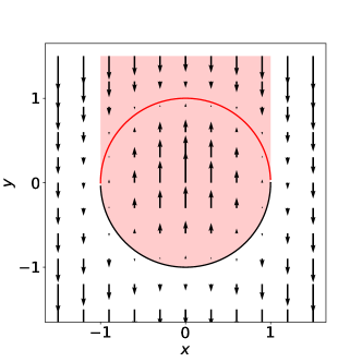 B.
B.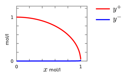
Example 16
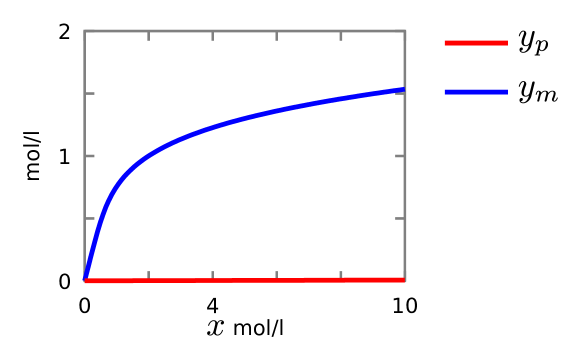
Even rather involved algebraic curves need surprisingly few species and reactions to be stabilized. This is the case of the serpentine curve, or anguinea, defined by the polynomial for which we choose the point to enforce stability. The compilation process takes less than 100ms on a typical laptop444An Ubuntu 20.04, with an Intel Core i6, GHz x cores and GB of memory.. The generated CRN reproduces the anguinea curve on the variable, as shown in Fig. 2. It is composed of the following species and reactions:
| (13) |
Example 17
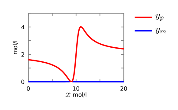
In the field of real analysis, the Bring radical of a real number is defined as the unique real root of the polynomial: . The Bring radical is an algebraic function of that cannot be expressed by any algebraic expression.
The stabilizing CRN generated by our compilation pipeline is composed of species (), where (resp. ) is the variable introduced to stabilized (resp. ) and the and subscripts represent the positive and negative parts of a signed variable, and reactions presented in model 14. A dose-response diagram of that CRN is shown in Fig. 3.
| (14) |
Example 18
To generate the CRN that stabilize the Hill function of order 5, we can use the
expression along with the point .
Our compilation pipeline generates the following model with species and
reactions:
| , | , |
| , | , |
| , | , | , |
| , | , | , |
all kinetics being mass action law with unit rate. The are auxiliary variables corresponding to the following expressions:
The production and degradation of may be surprising, but looking at all the reactions implying both and , we can see that their sum follow the equation hence ensuring that the sum of the two is driven back to , independently of their initial concentrations. It is worth remarking that another way of reaching the same result would be to directly build-in conservation laws into our CRN, hence using both steady state and invariant laws to define our steady state which however would make us sensitive to the initial concentrations.
6 Error control
An important aspect of our framework that we still do not have talked about is the ability to determine the error between the target function and the output of our synthesized CRN. Upon this section, we will adopt the following point of view. On the one hand, the system is supposed to be noiseless, meaning that both the auxiliary and the output variables exactly follow the PODE without any perturbations. On the other hand, the inputs are supposed to be driven by the environment in a way that we do not know in advance, thus fully determining the target function . We would like to have an estimation of the error between the output of the CRN and the target function:
| (15) |
Of course, this is possible only by assuming some regularity property of the input. For example, if we work with non-continuous input functions, just after a singularity of the inputs, the error may be arbitrarily large. But this does not seems fair as our output, as a solution of a PODE, will always be continuous. But even continuous functions are too liberal, since one can construct function that goes arbitrarily fast from one value to another, once again making our CRN unable to follow the pace.
To avoid this, we shall suppose that the inputs have a given maximal rate of change, or to say it mathematically, that all the input functions are -Lipschitz for a given : . Lipschitz functions are differentiable almost everywhere, and for each time where the inputs are differentiable, we have:
| (16) |
While this may seem a stringent requirement, it is actually quite natural to suppose that the concentration of chemical species cannot increase or decrease arbitrarily fast.
6.1 General case
For the sake of clarity, we shall derive the equations for a function of one variable and shall suppose without loss of generality that the input is differentiable everywhere.
To generalize to the case of functions of several variables, it is sufficient to sum the derivatives of with respect to all variables, thus providing an over approximation of the derivative with respect to any unitary vector.
To handle cases where the inputs is not differentiable everywhere, the argument we give here can be derived on every interval where the input is differentiable and the whole solution can be recovered by continuity.
We shall also focus on the mathematical framework of PODE where the output may be directly linked to the inputs and will study the case where we have to introduce variables to quadratize the polynomial later. Hence, given an input and a CRN stabilizing the output on the function . By definition, we have the polynomial of the curve . We thus have:
| (17) |
where , is a multiplicative constant that do not modify the stabilized function but allows for a faster convergence by increasing the kinetic turnover of the CRN. It is worth noting that due to the time varying inputs, equation 17 is technically a non-autonomous ODE, without modifying our reasoning.
We define the error as . Note that we define a signed error and allow to be negative. Differentiating with respect to time, we obtain:
| (18) |
The main unknown in this equation is but, let us remark that by its very definition, is null when . We can thus introduce a new polynomial that will be important for our error control:
| (19) |
Note that this is not an approximation but a definition of . A good property of is that it has to be positive in order to stabilize the desired branch, this explain why the symbol on the left hand side of the previous equation is replaced by a minus sign on the right.
Using the fact that has a well defined sign and that is Lipschitz and thus , equation (18) allows us to bound the derivative of . Gathering the upper and lower bounds in a single differential inequation we have:
| (20) |
This inequality is our central result as it allows to determine the sign of and thus the flow of the error. If the left hand side is positive, is increasing and if the right hand side is negative it is decreasing. In the third case, that is if the left and right hand side have different signs, we are not able to determine the sign of . Thus, this inequality (20) separates the space in different regions. The ones where the derivative is positive or negative for sure, and the one where we cannot determine its sign. These three regions are delimited by the two curves where the right and left hand side vanished that is:
| (21) |
A consequence of the flow of the differential inequation is that a system that start in the inner region where the sign is unknown will always stays in this region whatever the variation of the input, hence giving us an upper and lower bound on the output. The important parameter controlling this region is the ratio between the Lipschitz coefficient of the input and the kinetic turn-over since the error results from a kind of race between the target function controlled by , and the output controlled by . An interesting consequence is that the bounding becomes tighter when the input function stabilizes and decreases. The precise form of this region can be directly deduced from the polynomial .
This brings us to the notion of online control of the errorsout. If we are, when searching for a particular precision for the output given a constraint on the input to be Lipschitz, ensuring that . Looking on equation (21), we have to bound the right hand side. For this, we have to find a minimum to and a maximum to . To prevent these quantities from diverging on the boundaries of their domain, let us restrict ourself to a closed region .
Proposition 19
Proposition 20
For input functions that are -Lipschitz and a system in a closed region , we can define the quantity:
| (22) |
ensuring that for , we have: . That is, as soon as the precision is reached, it will be conserved at all time.
Before showing on an example the derivation of the stable region. Let us have a last glance on the equation (18) to discuss the transient response if the system start outside of the stable region defines by equation (21). Assuming that the system is nonetheless in the domain and will not diverge or reach another branch of the algebraic curve. The transient regime is important when the last term of equation (20) is negligible and thus, we will consider the case where , that is the inputs are fixed. The main argument now is that we have suppose that the polynomial was of multiplicity for the branch we want to stabilize, or said otherwise: is such that for all initial conditions , is not a root of . The direct consequence of this remark is that, at least locally around the solution, the convergence toward the stable region is always exponential with a characteristic time of the order of . A more rigorous proof of this assertion can be found in [16].
To sum up the behavior of a stabilizing CRN when the input functions are -Lipschitz. We first have a transient response of exponential decay toward the desired target function. And once the system enter into a region the shape of which is defined by and the width by the ratio , we know for sure that it will remains in this bounded region.
This gives a mitigate result for the precision, on one side we first have a fast increase in precision when the system is far from the target function because the exponential decay means that we gain one bit of precision at each time step (up to a multiplicative factor). But once we have reached the bounded region, as , each supplementary bit of precision asks for a factor in the kinetic turn-over which may represent a high energetic cost.
Example 21
To clarify the general case above, we will first develop our framework on the simplest case: . Thus , and we have:
| (23) | ||||
| (24) | ||||
| (25) |
We can then rewrite inequation (20) for this particular case:
| (26) |
Or taking directly the boundaries given by equation (21): . This gives a bounding interval for the output function:
| (27) |
The idea is that while the exact behaviour of the output is unknown without adding more constraints on the input, we can at least ensure this permissive bounding on the system as presented in figure 4A.
A. 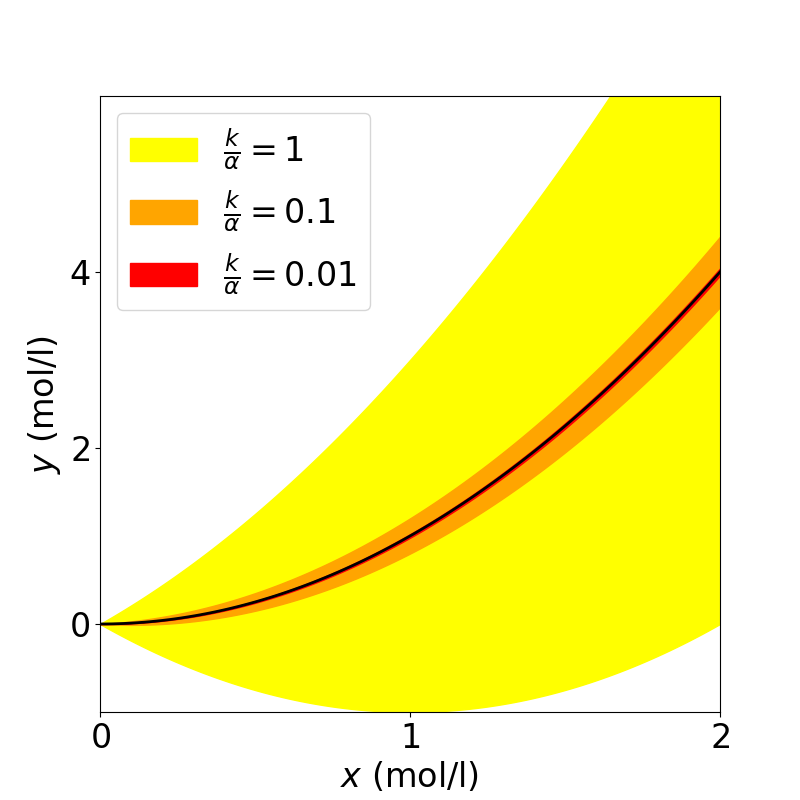 B.
B. 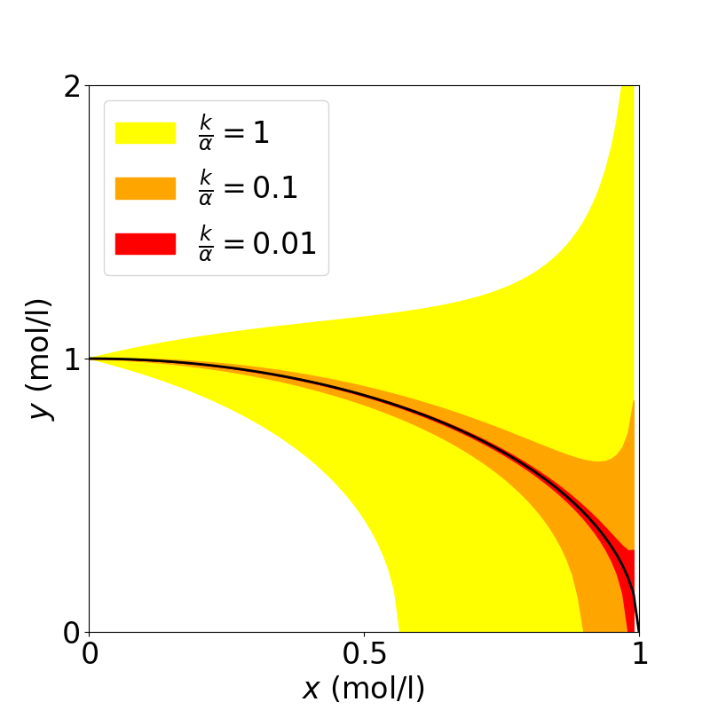
Example 22
Now we will look at the error control for the CRN stabilizing the circle already presented in example 15. We can easily derived the following relations for the main quantities:
| (28) |
Let us make a pause on the roots of () to note that they are all on the lower branch of the circle and thus outside of the domain . Hence validating the fact that we have an exponential convergence for all points inside the domain.
Now inserting the computed quantities into the general case equation (21), we have:
| (29) |
Solving this quadratic equation, we obtain the upper and lower error bounds which gives us a bounding for the output when the input is -Lipschitz:
| (30) |
As can be seen on figure 4B., a peculiar behaviour of this inequality is that there exists a region near where the lower bound is undefined. Intuitively, this is linked to the possibility, when close from the monodromy point of crossing the lower branch of the circle and from there the flow will drive the system to as it is no more on the domain (see fig. 1).
While these regions may appear quite large, they corresponds to a powerful notion of error control in the sense that they ensure a given precision for any k-Lipschitz input functions, which is a small constraint. Moreover, in practice, the error observed for typical input functions like offset sine waves are far smaller than the bounds given by our analysis.
6.2 Error control with intermediate species
Our main tool to transform the ODE so that they are amenable to a CRN implementation is through the introduction of new variables. This rises the question of how the final error is affected by this kind of transformation. We will not provide a full analysis of this phenomena in the general case but will build an intuition upon two basic examples corresponding to the two main cases where we have to introduce new variables: the quadratization when dealing with monomial of degree higher than and the polynomialization when the expression provided by the user is not directly a polynomial.
Example 23
We will start with the simplest case of quadratization taking as our direct case and as the chained case.
For the direct case we just repeat the computation of the previous subsections and immediately obtain:
| (31) |
For the quadratized case, we rely on the computation of the square case to obtain:
| (32) | ||||
and we can see that the first error term is the same as the one of the direct case why all the other ones are supplementary errors introduced by the quadratization, meaning that the quadratization is a net source of errors. This was expected as it introduces delay along the computation so that the output is less reactive to a variation of the input. The supplementary error introduced by the quadratization is especially important when and increasing the importance of the ratio between the regularity of the input and the kinetic turnover for quadratized systems.
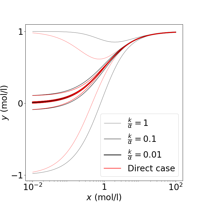
Example 24
A more involved case is the stabilization of the Hill function . While this case may seem somehow artificial as the direct implementation is possible and shows a better bounding on the error. The CRN with one variable added is actually simpler to implement when going to higher order hill functions and may effectively be produced by our algorithm depending on the way the expression is provided to the compiler (see example 2).
The simplest way to stabilize a hill function is thus through a direct implementation:
| (33) |
computing the error in this case is easy and we obtain:
| (34) |
But another path is to introduce the inverse of the hill function and use it to construct the desired output:
| (35) |
In this case, the error on is exactly the same as the computation of the direct path but this error is then passed on giving us a final error on the output:
| (36) |
which is, once again, strictly worse than the direct case as can be seen on figure 5. The error in the direct and indirect path are similar when the input is far from but in the region near the threshold of the hill function, the error of the indirect case may be far larger than the direct case. Moreover, it is impossible to increase to mitigate this effect as both cases scale similarly with respect to the kinetic turnover.
To conclude this section, using intermediate species to perform the computation is always detrimental in terms of error control. The two main sources of error being the amplification of intermediate errors and the computational delay making the output less sensitive to fast variations of the input functions.
While the first kind of errors may be handle through an increase of the kinetic turnover, which is important because of there prevalence in the quadratization scheme. The second kind cannot be reduced except by a better choice during the reduction of the expression to be compiled.
For now, our polynomialization algorithm does not incorporate any form of choice based on the scaling of the error but it could be interesting to see, when several polynomialization or quadratization are possible, if we could determine the ones producing the tighter region for the final output.
7 Conclusion and perspectives
We have introduced a notion of Absolute Functional Robustness for CRNs that compute a real function online, in the sense that the concentration of one output species continuously stabilizes to the result of some function of the input species concentrations, whatever changes are applied to the molecular concentrations within the domain of definition of the function. We have shown that the set of real functions that can be continuously stabilized by a CRN with mass action law kinetics is precisely the set of real algebraic functions.
Furthermore, by restricting the changes of the inputs to continuous changes with a rate bounded by some constant, i.e. by restricting to environment inputs driven by -Lipschitz functions, we were able to bound the error on the output by an analytic expression which can in principle be used to control the error.
While our main theorem focuses on CRNs at steady states, some important aspects of signal processing are linked to the timings of the signals. Our CRN stabilization framework relies on ratios between molecular production and degradation, and the error analysis we have done relates the possible multiplication of both terms by some factor to the characteristic time of relaxation, with . It is thus worth remarking in this respect that high value of filter out the high frequency noise of the inputs, while small values result in a more accurate output, yet at the expense of a higher molecular turnover.
These theoretical results open a whole research avenue for both the understanding of the structure of natural CRNs that allow cells to adapt to their environment, and for the design of artificial CRNs to implement in chemistry high-level functions that have to be maintained in moving environments. For these reasons, our online computational framework seems better suited than our earlier definition of functions computed by a CRN with fixed initial conditions [12], to both the formal study of natural CRNs in the perspective of systems biology, and the design of robust artificial CRNs in the perspective of synthetic biology.
The CRN compiler of algebraic functions we have implemented in Biocham according to these principles, automatically generates an abstract CRN. Implementing that abstract CRN with a concrete CRN using with real enzymes, as done e.g. in [8] for the making of protocellular biosensors, may depend on a non trivial way of the different choices made during the steps of polynomialization, dual-rail encoding and quadratization, rendering the final abstract CRN prone to a concrete implementation, or not. Taking into account a catalog of concrete enzymatic reactions earlier on in our compilation pipeline, i.e. during the polynomialization, quadratization and dual-rail encoding steps, is a particularly interesting challenge. First, from the point of view of the potential applications in the biomedical and environment domains, to guide search towards concrete economical solutions, but also from the point of view of the computational complexity of the computer algebra problems that need to be solved in our compilation scheme, e.g. for guiding search in our quadratization problem shown NP-hard in [19] and currently solved in practice using a MAXSAT solver.
Acknowledgments.
We are grateful to Amaury Pouly and Sylvain Soliman for preliminary discussions on this work, to the reviewers for their very insigthful comments, and to ANR-20-CE48-0002 Difference and Inria AEx GRAM grants for partial support.
References
- [1] H. J. Buisman, H. M. M. ten Eikelder, P. A. J. Hilbers, and A. M. L. Liekens. Computing algebraic functions with biochemical reaction networks. Artificial Life, 15(1):5–19, 2009.
- [2] Laurence Calzone, François Fages, and Sylvain Soliman. BIOCHAM: An environment for modeling biological systems and formalizing experimental knowledge. Bioinformatics, 22(14):1805–1807, 2006.
- [3] Luca Cardelli, Mirco Tribastone, and Max Tschaikowski. From electric circuits to chemical networks. Natural Computing, 19, 2020.
- [4] David C. Carothers, G. Edgar Parker, James S. Sochacki, and Paul G. Warne. Some properties of solutions to polynomial systems of differential equations. Electronic Journal of Differential Equations, 2005(40):1–17, 2005.
- [5] Vijayalakshmi Chelliah, Camille Laibe, and Nicolas Novère. Biomodels database: A repository of mathematical models of biological processes. In Maria Victoria Schneider, editor, In Silico Systems Biology, volume 1021 of Methods in Molecular Biology, pages 189–199. Humana Press, 2013.
- [6] Ho-Lin Chen, David Doty, and David Soloveichik. Deterministic function computation with chemical reaction networks. Natural computing, 7433:25–42, 2012.
- [7] Matthew Cook, David Soloveichik, Erik Winfree, and Jehoshua Bruck. Programmability of chemical reaction networks. In Anne Condon, David Harel, Joost N. Kok, Arto Salomaa, and Erik Winfree, editors, Algorithmic Bioprocesses, pages 543–584. Springer Berlin Heidelberg, Berlin, Heidelberg, 2009.
- [8] Alexis Courbet, Patrick Amar, François Fages, Eric Renard, and Franck Molina. Computer-aided biochemical programming of synthetic microreactors as diagnostic devices. Molecular Systems Biology, 14(4), 2018.
- [9] Gheorghe Craciun and Martin Feinberg. Multiple equilibria in complex chemical reaction networks: II. the species-reaction graph. SIAM Journal on Applied Mathematics, 66(4):1321–1338, 2006.
- [10] X. Duportet, L. Wroblewska, P. Guye, Y. Li, J. Eyquem, J. Rieders, G. Batt, and R. Weiss. A platform for rapid prototyping of synthetic gene networks in mammalian cells. Nucleic Acids Research, 42(21), 2014.
- [11] Péter Érdi and János Tóth. Mathematical Models of Chemical Reactions: Theory and Applications of Deterministic and Stochastic Models. Nonlinear science : theory and applications. Manchester University Press, 1989.
- [12] François Fages, Guillaume Le Guludec, Olivier Bournez, and Amaury Pouly. Strong Turing Completeness of Continuous Chemical Reaction Networks and Compilation of Mixed Analog-Digital Programs. In CMSB’17: Proceedings of the fiveteen international conference on Computational Methods in Systems Biology, volume 10545 of Lecture Notes in Computer Science, pages 108–127. Springer-Verlag, September 2017.
- [13] François Fages, Steven Gay, and Sylvain Soliman. Inferring reaction systems from ordinary differential equations. Theoretical Computer Science, 599:64–78, September 2015.
- [14] François Fages and Sylvain Soliman. Abstract interpretation and types for systems biology. Theoretical Computer Science, 403(1):52–70, 2008.
- [15] Martin Feinberg. Mathematical aspects of mass action kinetics. In L. Lapidus and N. R. Amundson, editors, Chemical Reactor Theory: A Review, chapter 1, pages 1–78. Prentice-Hall, 1977.
- [16] Willem Fletcher, Titus H Klinge, James I Lathrop, Dawn A Nye, and Matthew Rayman. Robust real-time computing with chemical reaction networks. In Unconventional Computation and Natural Computation: 19th International Conference, UCNC 2021, Espoo, Finland, October 18–22, 2021, Proceedings 19, pages 35–50. Springer, 2021.
- [17] V. Hárs and J. Tóth. On the inverse problem of reaction kinetics. In M. Farkas, editor, Colloquia Mathematica Societatis János Bolyai, volume 30 of Qualitative Theory of Differential Equations, pages 363–379, 1979.
- [18] Mathieu Hemery and François Fages. Algebraic biochemistry: a framework for analog online computation in cells. In CMSB’22: Proceedings of the twentieth international conference on Computational Methods in Systems Biology, volume 13447 of Lecture Notes in Computer Science. Springer-Verlag, September 2022.
- [19] Mathieu Hemery, François Fages, and Sylvain Soliman. On the complexity of quadratization for polynomial differential equations. In CMSB’20: Proceedings of the eighteenth international conference on Computational Methods in Systems Biology, Lecture Notes in Computer Science. Springer-Verlag, September 2020.
- [20] Mathieu Hemery, François Fages, and Sylvain Soliman. Compiling elementary mathematical functions into finite chemical reaction networks via a polynomialization algorithm for ODEs. In CMSB’21: Proceedings of the nineteenth international conference on Computational Methods in Systems Biology, volume 12881 of Lecture Notes in Computer Science. Springer-Verlag, September 2021.
- [21] Mathieu Hemery and Paul François. In silico evolution of biochemical log-response. The Journal of Physical Chemistry B, 2019.
- [22] Chi-Ying Huang and James E. Ferrell. Ultrasensitivity in the mitogen-activated protein kinase cascade. PNAS, 93(19):10078–10083, September 1996.
- [23] Michael Hucka et al. The systems biology markup language (SBML): A medium for representation and exchange of biochemical network models. Bioinformatics, 19(4):524–531, 2003.
- [24] Sarah M. Keating, Dagmar Waltemath, Matthias König, Fengkai Zhang, Andreas Dräger, Claudine Chaouiya, Frank T. Bergmann, Andrew Finney, Colin S. Gillespie, Tomás Helikar, Stefan Hoops, Rahuman S. Malik-Sheriff, Stuart L. Moodie, Ion I. Moraru, Chris J. Myers, Aurélien Naldi, Brett G. Olivier, Sven Sahle, James C. Schaff, Lucian P. Smith, Maciej J. Swat, Denis Thieffry, Leandro Watanabe, Darren J. Wilkinson, Michael L. Blinov, Kimberly Begley, James R. Faeder, Harold F. Gómez, Thomas M. Hamm, Yuichiro Inagaki, Wolfram Liebermeister, Allyson L. Lister, Daniel Lucio, Eric Mjolsness, Carole J. Proctor, Karthik Raman, Nicolas Rodriguez, Clifford A. Shaffer, Bruce E. Shapiro, Joerg Stelling, Neil Swainston, Naoki Tanimura, John Wagner, Martin Meier-Schellersheim, Herbert M. Sauro, Bernhard Palsson, Hamid Bolouri, Hiroaki Kitano, Akira Funahashi, Henning Hermjakob, John C. Doyle, Michael Hucka, Richard R. Adams, Nicholas A. Allen, Bastian R. Angermann, Marco Antoniotti, Gary D. Bader, Jan Cervený, Mélanie Courtot, Chris D. Cox, Piero Dalle Pezze, Emek Demir, William S. Denney, Harish Dharuri, Julien Dorier, Dirk Drasdo, Ali Ebrahim, Johannes Eichner, Johan Elf, Lukas Endler, Chris T. Evelo, Christoph Flamm, Ronan MT Fleming, Martina Fröhlich, Mihai Glont, Emanuel Gonçalves, Martin Golebiewski, Hovakim Grabski, Alex Gutteridge, Damon Hachmeister, Leonard A. Harris, Benjamin D. Heavner, Ron Henkel, William S. Hlavacek, Bin Hu, Daniel R. Hyduke, Hidde Jong, Nick Juty, Peter D. Karp, Jonathan R. Karr, Douglas B. Kell, Roland Keller, Ilya Kiselev, Steffen Klamt, Edda Klipp, Christian Knüpfer, Fedor Kolpakov, Falko Krause, Martina Kutmon, Camille Laibe, Conor Lawless, Lu Li, Leslie M. Loew, Rainer Machne, Yukiko Matsuoka, Pedro Mendes, Huaiyu Mi, Florian Mittag, Pedro T. Monteiro, Kedar Nath Natarajan, Poul MF Nielsen, Tramy Nguyen, Alida Palmisano, Jean-Baptiste Pettit, Thomas Pfau, Robert D. Phair, Tomas Radivoyevitch, Johann M. Rohwer, Oliver A. Ruebenacker, Julio Saez-Rodriguez, Martin Scharm, Henning Schmidt, Falk Schreiber, Michael Schubert, Roman Schulte, Stuart C. Sealfon, Kieran Smallbone, Sylvain Soliman, Melanie I. Stefan, Devin P. Sullivan, Koichi Takahashi, Bas Teusink, David Tolnay, Ibrahim Vazirabad, Axel Kamp, Ulrike Wittig, Clemens Wrzodek, Finja Wrzodek, Ioannis Xenarios, Anna Zhukova, and Jeremy Zucker. SBML level 3: an extensible format for the exchange and reuse of biological models. Molecular Systems Biology, 16(8):1–21, August 2020.
- [25] K. Oishi and E. Klavins. Biomolecular implementation of linear i/o systems. IET Systems Biology, 5(4):252–260, 2011.
- [26] Lulu Qian, David Soloveichik, and Erik Winfree. Efficient turing-universal computation with DNA polymers. In Proc. DNA Computing and Molecular Programming, volume 6518 of LNCS, pages 123–140. Springer-Verlag, 2011.
- [27] Lee A. Segel. Modeling dynamic phenomena in molecular and cellular biology. Cambridge University Press, 1984.
- [28] Guy Shinar and Martin Feinberg. Structural sources of robustness in biochemical reaction networks. Science, 327(5971):1389–1391, 2010.
- [29] Marko Vasic, David Soloveichik, and Sarfraz Khurshid. CRN++: Molecular programming language. In Proc. DNA Computing and Molecular Programming, volume 11145 of LNCS, pages 1–18. Springer-Verlag, 2018.