Abstract

Data preprocessing is a crucial part of any machine learning pipeline, and it can have a significant impact on both performance and training efficiency. This is especially evident when using deep neural networks for time series prediction and classification: real-world time series data often exhibit irregularities such as multi-modality, skewness and outliers, and the model performance can degrade rapidly if these characteristics are not adequately addressed. In this work, we propose the EDAIN (Extended Deep Adaptive Input Normalization) layer, a novel adaptive neural layer that learns how to appropriately normalize irregular time series data for a given task in an end-to-end fashion, instead of using a fixed normalization scheme. This is achieved by optimizing its unknown parameters simultaneously with the deep neural network using back-propagation. Our experiments, conducted using synthetic data, a credit default prediction dataset, and a large-scale limit order book benchmark dataset, demonstrate the superior performance of the EDAIN layer when compared to conventional normalization methods and existing adaptive time series preprocessing layers.

1 INTRODUCTION

There are many steps required when applying deep neural networks or, more generally, any machine learning model, to a problem. First, data should be gathered, cleaned, and formatted into machine-readable values. Then, these values need to be preprocessed to facilitate learning. Next, features are designed from the processed data, and the model architecture and its hyperparameters are chosen. This is followed by parameter optimisation and evaluation using suitable metrics. These steps may be iterated several times.

A step that is often overlooked in the literature is preprocessing (see, for example, Koval,, 2018), which consists in operations used to transform raw data in a format that is suitable for further modeling, such as detecting outliers, handling missing data and normalizing features. Applying appropriate preprocessing to the data can have significant impact on both performance and training efficiency (Cao et al.,, 2018; Nawi et al.,, 2013; Passalis et al.,, 2020; Sola and Sevilla,, 1997; Tran et al.,, 2021). However, determining the most suitable preprocessing method usually requires a substantial amount of time and relies on iterative training and performance testing. Therefore, the main objective of this work is to propose a novel efficient automated data preprocessing method for optimising the predictive performance of neural networks, with a focus on normalization of multivariate time series data.

1.1 Preprocessing multivariate time series

Let $\mathcal{D}=\left\{\mathbf{X}^{(i)}\in\mathbb{R}^{d\times T},\ i=1,\dots,N\right\}$ denote a dataset containing $N$ time series, where each time series $\mathbf{X}^{(i)}\in\mathbb{R}^{d\times T}$ is composed of $T$ $d$-dimensional feature vectors. The integers $d$ and $T$ refer to the feature and temporal dimensions of the data, respectively. Also, we use $\mathbf{x}^{(i)}_{t}\in\mathbb{R}^{d},\ t=1,\dots,T$ to refer to the $d$ features observed at timestep $t$ in the $i$-th time series. Before feeding the data into a model such as a deep neural network, it is common for practitioners to perform $z$-score normalization (see, for example, Koval,, 2018) on $\mathbf{x}^{(i)}_{t}=(x^{(i)}_{t,1},\dots,x^{(i)}_{t,d})\in\mathbb{R}^{d}$, obtaining

$$\tilde{x}^{(i)}_{t,k}=\frac{x^{(i)}_{t,k}-\mu_{k}}{\sigma_{k}},\ k=1,\dots,d,$$ (1)

where $\mu_{k}$ and $\sigma_{k}$ denote the mean and standard deviation of the measurements from the $k$-th predictor variable. Another commonly used method is min-max scaling, where the observations for each predictor variable are transformed to fall in the value range $[0,1]$ (see, for example, Koval,, 2018). In this work, we refer to these conventional methods as static preprocessing methods, as the transformation parameters are fixed statistics that are computed through a single sweep of the training data. Most of these transformations only change the location and scale of the observations, but real-world data often contains additional irregularities such as skewed distributions, outliers, extreme values, heavy tails and multiple modes (Cao et al.,, 2023; Nawi et al.,, 2013), which are not mitigated by transformations such as $z$-score and min-max normalization. Employing static normalization in such cases may lead to sub-optimal results, as demonstrated in Passalis et al., (2020, 2021); Tran et al., (2021) and in the experiments on real and synthetic data in Section 4 of this work.

In contrast, better results are usually obtained by employing adaptive preprocessing methods (see, for example Lubana et al.,, 2021; Passalis et al.,, 2020, 2021; Tran et al.,, 2021), where the preprocessing is integrated into the deep neural network by augmenting its architecture with additional layers. Both the transformation parameters and the neural network model parameters are then jointly optimised in an end-to-end fashion as part of the objective function of interest. The main contribution of this this paper belongs to this class of methods: we propose a novel adaptive normalization approach, called EDAIN (Extended Deep Adaptive Input Normalization), which can appropriately handle irregularities in the input data, without making any assumption on their distribution.

1.2 Contributions

The main contribution of our work is EDAIN, displayed in Figure 1, a neural layer that can be added to any neural network architecture for preprocessing multivariate time series. This method complements the shift and scale layers proposed in DAIN (Passalis et al.,, 2020, described in details in Section 2) with an adaptive outlier mitigation sublayer and a power transform sublayer, used to handle common irregularities observed in real-world data, such as outliers, heavy tails, extreme values and skewness.

Additionally, our EDAIN method can be implemented in two versions, named global-aware and local-aware, suited to unimodal and multi-modal data respectively. Furthermore, we propose a computationally efficient variation of EDAIN, trained via the Kullback-Leibler divergence, named EDAIN-KL. Like EDAIN, this method can normalize skewed data with outliers, but in an unsupervised fashion, and can be used in conjunction with non-neural-network models.

EDAIN is described in details in Section 3, after a discussion on related methods in Section 2. The proposed methodology is extensively evaluated on synthetic and real-world data in Section 4, followed by a discussion on its performance and a conclusion. An open-source implementation of the EDAIN layer, along with code for reproducing the experiments, is available in the GitHub repository marcusGH/edain_paper.

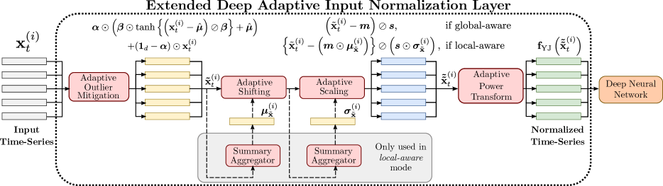
Figure 1: Architecture of the proposed EDAIN (Extended Deep Adaptive Input Normalization) layer. The layout and color choices of the diagram are based on Figure 1 from Passalis et al., (2020).

2 RELATED WORK

Several works consider adaptive normalization methods, but they all apply the normalization transformation to the outputs of the inner layers within the neural network, known as activations in the literature. A well-known example of these transformations is batch normalization (Ioffe and Szegedy,, 2015), which applies $z$-score normalization to the output of each inner layer, but several alternatives and extensions exist (see, for example, Huang et al.,, 2023; Lubana et al.,, 2021; Yu and Spiliopoulos,, 2023). To the best of our knowledge, there are only three other methods where the deep neural network is augmented by inserting the adaptive preprocessing layer as the first step, transforming the data before it enters the network: the Deep Adaptive Input Normalization (DAIN) layer Passalis et al., (2020), the Robust Deep Adaptive Input Normalization (RDAIN) layer Passalis et al., (2021), and the Bilinear Input Normalization (BIN) layer Tran et al., (2021). We will describe the DAIN layer in more detail in the next paragraph, as this method resembles our proposed EDAIN method the most.

The DAIN layer normalizes each time series $\mathbf{X}^{(i)}$ using three sublayers: each time series is first shifted, then scaled, and finally passed through a gating layer that can suppress irrelevant features. The unknown parameters are the weight matrices $\mathbf{W}_{a}$, $\mathbf{W}_{b}$, $\mathbf{W}_{c}\in\mathbb{R}^{d\times d}$, and the bias term $\mathbf{d}\in\mathbb{R}^{d}$, and are used for the shift, scale, and gating sublayer, respectively. The first two layers together, perform the operation

$$\tilde{\mathbf{x}}_{t}^{(i)}=\left(\mathbf{x}_{t}^{(i)}-\mathbf{W}_{a}\mathbf{a}^{(i)}\right)\oslash\mathbf{W}_{b}\mathbf{b}^{(i)},$$ (2)

where $\mathbf{x}_{t}^{(i)}\in\mathbb{R}^{d}$ is the input feature vector at timestep $t$ of time series $i$, $\oslash$ denotes element-wise division, and $\mathbf{a}^{(i)}\in\mathbb{R}^{d}$ and $\mathbf{b}^{(i)}\in\mathbb{R}^{d}$ are summary statistics that are computed for the $i$-th time series as follows:

$$\mathbf{a}^{(i)}=\frac{1}{T}\sum^{T}_{t=1}\mathbf{x}_{t}^{(i)},\ \mathbf{b}^{(i)}=\sqrt{\frac{1}{T}\sum^{T}_{t=1}\left(\mathbf{x}^{(i)}_{t}-\mathbf{W}_{a}\mathbf{a}^{(i)}\right)^{2}}.$$ (3)

In Equation (3), the power operations are applied element-wise. The third sublayer, the gating layer, performs the operation

$$\tilde{\tilde{\mathbf{x}}}_{t}^{(i)}=\tilde{\mathbf{x}}^{(i)}_{t}\odot S\left(\mathbf{W}_{c}\mathbf{c}^{(i)}+\mathbf{d}\right).$$ (4)

Here, $\odot$ is the element-wise multiplication operator, $S:\mathbb{R}^{d}\to\mathbb{R}^{d}$ denotes the logistic function applied element-wise, and $\mathbf{c}^{(i)}$ is the summary statistic

$$\mathbf{c}^{(i)}=\frac{1}{T}\sum^{T}_{t=1}\tilde{\mathbf{x}}_{t}^{(i)}.$$ (5)

The final output of the DAIN layer is thus

$$\tilde{\tilde{\mathbf{X}}}^{(i)}=\left[\tilde{\tilde{\mathbf{x}}}^{(i)}_{1},\dots,\tilde{\tilde{\mathbf{x}}}^{(i)}_{T}\right]\in\mathbb{R}^{d\times T}.$$ (6)

In the RDAIN layer proposed by Passalis et al., (2021), a similar 3-stage normalization pipeline as that of the DAIN layer is used, but a residual connection across the shift and scale sublayers is also introduced. The BIN layer (Tran et al.,, 2021) has two sets of linear shift and scale sublayers that work similarly to the DAIN layer, which are applied across columns and rows of each time series $\mathbf{X}^{(i)}\in\mathbb{R}^{d\times T}$. The output of the BIN layer is a trainable linear combination of the two.

In real world applications, data often present additional irregularities, such as outliers, extreme values, heavy tails and skewness, which the aforementioned adaptive preprocessing methods are not designed to handle. Therefore, this work proposes EDAIN, a layer which comprises two novel sublayers that can appropriately treat skewed and heavy-tailed data with outliers and extreme values, resulting in significant improvements in performance metrics on real and simulated data. Also, the DAIN, RDAIN and BIN adaptive preprocessing methods are only primarily designed to handle multi-modal and non-stationary time series, which are common in financial forecasting tasks (Passalis et al.,, 2020). They do this by making the shift and scale parameters a parameterised function of each $\mathbf{X}^{(i)}$, allowing a transformation specific to each time series data point, henceforth referred to as local-aware preprocessing. However, these normalization schemes do not necessarily preserve the relative ordering between time series data points, which can degrade performance on unimodal datasets. As discussed in the next section, we address this drawback by proposing a novel global-aware version for our proposed EDAIN layer, which preserves ordering by learning a monotonic transformation. It must be remarked that the EDAIN layer can also be fitted in local-aware fashion, to address multi-modality when present, providing additional flexibility when modelling real-world data.

3 EXTENDED DEEP ADAPTIVE INPUT NORMALIZATION

In this section, we describe in detail the novel EDAIN preprocessing layer, which can be added to any deep learning architecture for time series data. EDAIN adaptively applies local transformations specific to each time series, or global transformations across all the observed time series $\mathbf{X}^{(i)},\ i=1,\dots,N$ in the dataset $\mathcal{D}$. These transformations are aimed at appropriately preprocessing the data, mitigating the effect of skewness, outliers, extreme values and heavy-tailed distributions. This section discusses in details the different sublayers of EDAIN, its global-aware and local-aware versions, and training strategies via stochastic gradient descent or Kullback-Leibler divergence minimization.

An overview of the EDAIN layer’s architecture is shown in Figure 1. Given some input time series $\mathbf{X}^{(i)}\in\mathbb{R}^{d\times T}$, each feature vector $\mathbf{x}^{(i)}_{t}\in\mathbb{R}^{d}$ is independently transformed sequentially in four stages: an outlier mitigation operation $\mathbf{h}_{1}:\mathbb{R}^{d}\rightarrow\mathbb{R}^{d}$, a shift operation: $\mathbf{h}_{2}:\mathbb{R}^{d}\rightarrow\mathbb{R}^{d}$, a scale operation: $\mathbf{h}_{3}:\mathbb{R}^{d}\rightarrow\mathbb{R}^{d}$, and a power transformation operation: $\mathbf{h}_{4}:\mathbb{R}^{d}\rightarrow\mathbb{R}^{d}$.

Outlier mitigation sublayer.

In the literature, it has been shown that an appropriate treatment of outliers and extreme values can increase predictive performance (Yin and Liu,, 2022). The two most common ways of doing this are omission and winsorization (Nyitrai and Virág,, 2019). The former corresponds to removing the outliers from further analysis, whereas the latter seeks to replace outliers with a censored value corresponding to a given percentile of the observations. In this work we propose the following smoothed winsorization operation obtained via the $\tanh(\cdot)$ function:

$$\breve{\mathbf{x}}_{t}^{(i)}=\bm{\beta}\odot\tanh\left\{\left(\mathbf{x}_{t}^{(i)}-\hat{\bm{\mu}}\right)\oslash\bm{\beta}\right\}+\hat{\bm{\mu}},$$ (7)

where the parameter $\bm{\beta}\in[\beta_{\text{min}},\infty)^{d}$ controls the range to which the measurements are restricted to, and $\hat{\bm{\mu}}\in\mathbb{R}^{d}$ is the global mean of the data, considered as a fixed constant. In this work, we let $\beta_{\text{min}}=1$. Additionally, we consider a ratio of winsorization to apply to each predictor variable, controlled by an unknown parameter vector $\bm{\alpha}\in[0,1]^{d}$, combined with the smoothed winsorization operator (7) via a residual connection. This gives the following adaptive outlier mitigation operation for an input time series $\mathbf{x}_{t}^{(i)}\in\mathbb{R}^{d}$:

$$\mathbf{h}_{1}\left(\mathbf{x}_{t}^{(i)}\right)=\bm{\alpha}\odot\breve{\mathbf{x}}_{t}^{(i)}+\left(\bm{1}_{d}-\bm{\alpha}\right)\odot\mathbf{x}_{t}^{(i)},$$ (8)

where $\bm{1}_{d}$ is a $d$-dimensional vector of ones. Both $\bm{\alpha}$ and $\bm{\beta}$ are considered as unknown parameters as part of the full objective function optimised during training.

Shift and scale sublayers.

The adaptive shift and scale layer, combined, perform the operation

$$\mathbf{h}_{3}\left\{\mathbf{h}_{2}\left(\mathbf{x}_{t}^{(i)}\right)\right\}=(\mathbf{x}_{t}^{(i)}-\bm{m})\oslash\bm{s},$$ (9)

where the unknown parameters are $\bm{m}\in\mathbb{R}^{d}$ and $\bm{s}\in(0,\infty)^{d}$. Note that the EDAIN scale and shift sublayers generalise $z$-score scaling, which does not treat $\bm{m}$ and $\bm{s}$ as unknown parameters, but it sets them to the mean and standard deviation instead:

$$\bm{m}=\frac{1}{NT}\sum^{N}_{i=1}\sum^{T}_{t=1}\mathbf{x}_{t}^{(i)},$$ (10)

and

$$\bm{s}=\sqrt{\frac{1}{NT}\sum^{N}_{i=1}\sum^{T}_{t=1}\left(\mathbf{x}_{t}^{(i)}-\bm{m}\right)^{2}},$$ (11)

where the power operations are applied element-wise.

Power transform sublayer.

Many real-world datasets exhibit significant skewness, which is often corrected using power transformations (Schroth and Muma,, 2021), such as the commonly used Box-Cox transformation (Box and Cox,, 1964). One of the main limitations of the Box-Cox transformation is that it is only valid for positive values. A more general alternative which is more widely applicable is the Yeo-Johnson (YJ) transform (Yeo and Johnson,, 2000):

$$f_{\textrm{YJ}}^{\lambda}(x)=\left\{\begin{array}[]{ll}\frac{(x+1)^{\lambda}-1}{\lambda}&\textrm{if }\lambda\neq 0,\ x\geq 0,\\ \log(x+1)&\textrm{if }\lambda=0,\ x\geq 0,\\ \frac{(1-x)^{2-\lambda}-1}{\lambda-2}&\textrm{if }\lambda\neq 2,\ x<0,\\ -\log(1-x)&\textrm{if }\lambda=2,\ x<0.\end{array}\right.$$ (12)

The transformation $f_{\textrm{YJ}}^{\lambda}$ only has one unknown parameter, $\lambda\in\mathbb{R}$, and it can be applied to any $x\in\mathbb{R}$, not just positive values (Yeo and Johnson,, 2000). The power transform sublayer of EDAIN simply applies the transformation in Equation (12) along each dimension of the input time series $\mathbf{X}^{(i)}$. That is, for each $i=1,\dots,N$ and $t=1,\dots,T$, the sublayer outputs

$$\mathbf{h}_{4}\left(\mathbf{x}_{t}^{(i)}\right)=\left[f^{\lambda_{1}}_{\textrm{YJ}}\left(x_{t,1}^{(i)}\right),\dots,f^{\lambda_{d}}_{\textrm{YJ}}\left(x_{t,d}^{(i)}\right)\right],$$ (13)

where the unknown quantities to be optimised are the power parameters $\bm{\lambda}=(\lambda_{1},\dots,\lambda_{d})\in\mathbb{R}^{d}$.

3.1 Global- and local-aware normalization

For highly multi-modal and non-stationary time series data, Passalis et al., (2020, 2021) and Tran et al., (2021) observed significant performance improvements when using local-aware preprocessing methods, as these allow forming a unimodal representation space from predictor variables with multi-modal distributions. Therefore, we also propose a local-aware version of the EDAIN layer in addition to the global-aware version we presented earlier. In the local-aware version of EDAIN, the shift and scale operations also depend on a summary representation of the current time series $\mathbf{X}^{(i)}$ to be preprocessed:

$$\mathbf{h}_{3}\left\{\mathbf{h}_{2}\left(\mathbf{x}_{t}^{(i)}\right)\right\}=\left\{\mathbf{x}_{t}^{(i)}-\left(\bm{m}\odot\bm{\mu}_{\mathbf{x}}^{(i)}\right)\right\}\oslash\left(\bm{s}\odot\bm{\sigma}_{\mathbf{x}}^{(i)}\right).$$ (14)

The summary representations $\bm{\mu}_{\mathbf{x}}^{(i)},\bm{\sigma}_{\mathbf{x}}^{(i)}\in\mathbb{R}^{d}$, are computed through a reduction along the temporal dimension of each time series $\mathbf{X}^{(i)}$ (cf. Figure 2):

$$\bm{\mu}_{\mathbf{x}}^{(i)}=\frac{1}{T}\sum^{T}_{t=1}\mathbf{x}^{(i)}_{t},\ \bm{\sigma}_{\mathbf{x}}^{(i)}=\sqrt{\frac{1}{T}\sum^{T}_{t=1}\left(\mathbf{x}^{(i)}_{t}-\bm{\mu}_{\mathbf{x}}^{(i)}\right)^{2}},$$ (15)

where the power operations are applied element-wise in (15). The outlier mitigation and power transform sublayers remain the same for the local-aware version, except the $\hat{\bm{\mu}}$ statistic in Equation (7) is no longer fixed, but rather the mean of the input time series:

$$\hat{\bm{\mu}}^{(i)}=\frac{1}{T}\sum_{t=1}^{T}\mathbf{x}_{t}^{(i)}.$$ (16)

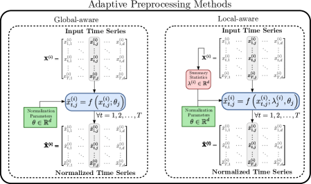
Figure 2: Visual comparison of the local- and global-aware versions of adaptive preprocessing schemes.

Order preservation.

Adaptive local-aware preprocessing methods work well on multi-modal data such as financial forecasting datasets (Passalis et al.,, 2020, 2021; Tran et al.,, 2021). However, as we will experimentally demonstrate in the next section, local-aware preprocessing methods might perform worse than conventional methods such as $z$-score normalization when applied to unimodal data. This is because local-aware methods are not order preserving, since the shift and scale amount is different for each time series. In many applications in which the features have a natural and meaningful ordering, it would be desirable to have

$$\tilde{x}^{(i)}_{t,k}<\tilde{x}^{(j)}_{t,k}\ \mathrm{if}\ x^{(i)}_{t,k}<x^{(j)}_{t,k},$$ (17)

for all $i,j\in\{1,\dots,N\}$, $t=1,\dots,T$ and $k=1,\dots,d$, where $\tilde{\mathbf{X}}^{(i)}$ denotes the output of a transformation with $\mathbf{X}^{(i)}$ as input. This property does not necessarily hold for the local-aware methods (DAIN, RDAIN, BIN, and local-aware EDAIN). For unimodal features, the qualitative interpretation of the predictor variables might dictate that property (17) should be maintained (for example, consider the case of credit scores for a default prediction application, cf. Section 4.2).

As a solution, the proposed global-aware version of the proposed EDAIN layer does not use any time series specific summary statistics, which makes each of the four sublayers monotonically non-decreasing. This ensures that property (17) is maintained by the global-aware EDAIN transformation, providing additional flexibility for applications on real world data where ordering within features should be preserved.

3.2 Optimising the EDAIN layer

The output of the proposed EDAIN layer is obtained by feeding the input time series $\mathbf{X}^{(i)}$ through the four sublayers in a feed-forward fashion, as shown in Figure 1. The output is then fed to the deep neural network used for the task at hand. Letting $\mathbf{W}$ denote the weights of the deep neural network model, the weights of both the deep model and the EDAIN layer are simultanously optimised in an end-to-end manner using stochastic gradient descent, with the update equation:

$$\Delta\left(\bm{\alpha},\bm{\beta},\bm{m},\bm{s},\bm{\lambda},\mathbf{W}\right)=\\ -\eta\bigg{(}\eta_{1}\frac{\partial\mathcal{L}}{\partial\bm{\alpha}},\eta_{1}\frac{\partial\mathcal{L}}{\partial\bm{\beta}},\eta_{2}\frac{\partial\mathcal{L}}{\partial\bm{m}},\eta_{3}\frac{\partial\mathcal{L}}{\partial\bm{s}},\eta_{4}\frac{\partial\mathcal{L}}{\partial\bm{\lambda}},\frac{\partial\mathcal{L}}{\partial\mathbf{W}}\bigg{)},$$ (18)

where $\eta\in(0,\infty)$ is the base learning rate, whereas $\eta_{1},\dots,\eta_{4}$ correspond to sublayer-specific corrections to the global learning rate $\eta$. As Passalis et al., (2020) observed when training their DAIN layer, the gradients of the unknown parameters for the different sublayers might have vastly different magnitudes, which prevents a smooth convergence of the preprocessing layer. Therefore, they proposed using separate learning rates for the different sublayers. We therefore introduce corrections $\eta_{\ell}\in\mathbb{R},\ \ell=\{1,2,3,4\}$ as additional hyperparameters that modify the learning rates for each of the four different EDAIN sublayers.

Furthermore, note that computing the fixed constant $\hat{\bm{\mu}}$ in the outlier mitigation sublayer (7) would require a sweep on the entire dataset before training the EDAIN-augmented neural network architecture, which could be computationally extremely expensive. As a solution to circumvent this issue, we propose to calculate $\hat{\bm{\mu}}$ iteratively during training, updating it using a cumulative moving average estimate at each forward pass of the sublayer. We provide more details on this in Section 1 of the supplementary material.

3.3 EDAIN-KL

In addition to the EDAIN layer, we also propose another novel preprocessing method, named EDAIN-KL (Extended Deep Adaptive Input Normalization, optimised with Kullback-Leibler divergence). This approach uses a similar neural layer architecture as the EDAIN method, but modifies it to ensure the transformation is invertible. Its unknown parameters are then optimised with an approach inspired by normalizing flows (see, for example, Kobyzev et al.,, 2021).

The EDAIN-KL layer is used to transform a Gaussian base distribution $\mathbf{Z}\sim\mathcal{N}(\bm{0},I_{dT})$ via a composite function $\mathbf{g}_{\bm{\theta}}=\mathbf{h}_{1}^{-1}\circ\mathbf{h}_{2}^{-1}\circ\mathbf{h}_{3}^{-1}\circ\mathbf{h}_{4}^{-1}$ comprised of the inverses of the operations in the EDAIN sublayers, applied sequentially with parameter $\bm{\theta}=(\bm{\alpha},\bm{\beta},\bm{m},\bm{s},\bm{\lambda})$. The parameter $\bm{\theta}$ is chosen to minimize the KL-divergence between the resulting distribution $\mathbf{g}_{\bm{\theta}}(\mathbf{Z})$ and the empirical distribution of the dataset $\mathcal{D}$:

$$\hat{\bm{\theta}}=\operatorname*{argmin}_{\bm{\theta}}\mathrm{KL}\left\{\mathcal{D}\ ||\ \mathbf{g}_{\bm{\theta}}(\mathbf{Z})\right\}.$$ (19)

Note that we apply all the operations in reverse order, compared to the EDAIN layer, because we use $\mathbf{g}_{\bm{\theta}}$ to transform a base distribution $\mathbf{Z}$ into a distribution that resembles the training dataset $\mathcal{D}$. To normalize the dataset after fitting the EDAIN-KL layer, we apply

$$\mathbf{g}^{-1}_{\hat{\bm{\theta}}}=\mathbf{h}_{4}\circ\mathbf{h}_{3}\circ\mathbf{h}_{2}\circ\mathbf{h}_{1}$$ (20)

to each $\mathbf{X}^{(i)}\in\mathbb{R}^{d\times T}$, similarly to the EDAIN layer. The main advantage of the EDAIN-KL approach over standard EDAIN is that it allows training in an unsupervised fashion, separate from the deep model. This enables its usage for preprocessing data in a wider set of tasks, including non-deep-neural-network models. An exhaustive description of the EDAIN-KL method is provided in Section 2 of the supplementary material.

4 EXPERIMENTAL EVALUATION

For evaluating the proposed EDAIN layer we consider a synthetic dataset, a large-scale default prediction dataset, and a large-scale financial forecasting dataset. We compare the two versions of the EDAIN layer (global-aware and local-aware) and the EDAIN-KL layer to $z$-score normalization, to the DAIN (Passalis et al.,, 2020) layer and to the BIN (Tran et al.,, 2021) layer. For all experiments, we use a recurrent neural network (RNN) model composed of gated recurrent unit (GRU) layers, followed by a classifier head with fully connected layers. Categorical features, when present, are passed through an embedding layer, whose output is combined with the output of the GRU layers and then fed to the classifier head. Full details on the model architectures, optimization procedures, including learning rates and number of epochs, can be found in Section 3 of the supplementary material and in the code repository associated with this work.

4.1 Synthetic Datasets

Before considering real-world data, we evaluate our method on synthetic data, where we have full control over the data generating process. To do this, we develop a synthetic time series data generation algorithm which allows specifying arbitrary unnormalized probability density functions (PDFs) for each of the $d$ predictor variables. It then generates $N$ time series of the form $\mathbf{X}^{(i)}\in\mathbb{R}^{d\times T}$, along with $N$ binary response variables ${y}^{(i)}\in\{0,1\}$. We present a detailed description of the algorithm in Section 4 of the supplementary material.

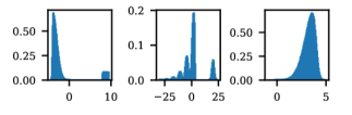
Figure 3: Histogram across timesteps $t=1,\dots,T$ of the $d=3$ predictor variables from the synthetic data.

For our experiments, we generated $N_{\mathcal{D}}=100$ datasets, each with $N=50\,000$ time series of length $T=10$ and dimensionality $d=3$. The three predictor variables were configured to be distributed as follows:

$$f_{1}(x)= \ 10\cdot\Phi_{\mathcal{N}}\left\{10\left(x+4\right)\right\}\cdot p_{\mathcal{N}}(x+4)$$

$$+\mathbb{I}_{(8,9.5)}(x)\cdot e^{x-8}/10,$$ (21)

$$f_{2}(x)= \left\{\begin{array}[]{ll}20\cdot p_{\mathcal{N}}(x-20),&\textrm{ if }x>\pi,\\ e^{x/6}\cdot\left\{10\sin(x)+10\right\},&\textrm{ if }x\leq\pi,\end{array}\right.$$ (24)

$$f_{3}(x)= \ 2\cdot\Phi_{\mathcal{N}}\left\{-4(x-4)\right\}\cdot p_{\mathcal{N}}(x-4),$$ (25)

where $p_{\mathcal{N}}(\cdot)$ and $\Phi_{\mathcal{N}}(\cdot)$ denote the PDF and cumulative distribution function (CDF) of the standard normal distribution, and $\mathbb{I}_{\mathcal{A}}(\cdot)$ is the indicator function on the set $\mathcal{A}$. Samples from the dataset are visualised in Figure 3. We train and evaluate a RNN model with the architecture described earlier on each of the $N_{\mathcal{D}}$ datasets using a 80%-20% train-validation split. Our results are presented in Table 1, where the binary cross-entropy (BCE) loss and the accuracy on the validation set are used as evaluation metrics.

From our experiments on the synthetic datasets, we observe that the model performance is more unstable when no preprocessing is applied, as seen from the increased variance in Table 1. We also observe that $z$-score normalization only gives minor performance improvements when compared to no preprocessing, aside from reducing the variance. As we have perfect information about the underlying data generation mechanism from Equations (21), (24) and (25), we also compared our methods to what we refer to as CDF inversion, where each observation is transformed by the CDF of its corresponding distribution, and then transformed via $\Phi_{\mathcal{N}}^{-1}(\cdot)$, giving predictor variables with standard normal distributions. We also apply this method to the real-world datasets in Section 4.2 and Section 4.3, but since the true PDFs are unknown in those settings, we estimate the CDFs using quantiles from the distribution of the training data. Out of all the methods not using information about the underlying data generation mechanism, the global-aware version of EDAIN demonstrates superior performance. It also almost performs as well as CDF inversion, which is able to perfectly normalize each predictor variable via its data generation mechanism. Finally, we observe that the local-aware methods perform even worse than no preprocessing: this might be due to the ordering not being preserved, as discussed in Section 3.1.

Preprocessing method	BCE loss	Binary accuracy (%)
No preprocessing	$0.1900\pm 0.0362$	$91.68\pm 1.68$
$z$-score normalization	$0.1873\pm 0.0108$	$91.73\pm 0.65$
CDF inversion	$\underline{0.1627\pm 0.0094}$	$\underline{92.89\pm 0.55}$
EDAIN-KL	$0.1760\pm 0.0094$	$92.24\pm 0.59$
EDAIN (local-aware)	$0.2099\pm 0.0095$	$90.71\pm 0.57$
EDAIN (global-aware)	$\mathbf{0.1636\pm 0.0086}$	$\mathbf{92.83\pm 0.51}$
BIN	$0.2191\pm 0.0103$	$90.36\pm 0.59$
DAIN	$0.2153\pm 0.0146$	$90.48\pm 0.78$

Table 1: Experimental results on synthetic data, with 95% normal confidence intervals $(\mu\pm 1.96\sigma)$ calculated across $N_{\mathcal{D}}=100$ datasets. The gold-standard method for this simulation (CDF inversion) is underlined.

4.2 Default Prediction Dataset

The first real-world dataset we consider is the publicly available default prediction dataset published by American Express (Howard et al.,, 2022), which contains data from $N=458\,913$ credit card customers. For each customer, a vector of $d=188$ aggregated profile features has been recorded at $T=13$ different credit card statement dates, producing a multivariate time series of the form $\mathbf{X}^{(i)}\in\mathbb{R}^{d\times T},\ i=1,2,\dots,N$. Given $\mathbf{X}^{(i)}$, the task is to predict a binary label $y^{(i)}\in\{0,1\}$ indicating whether the $i$-th customer defaulted at any point within 18 months after the last observed data point in the time series. A default event is defined as not paying back the credit card balance amount within 120 days after the latest statement date (Howard et al.,, 2022). Out of the $d=188$ features, only the 177 numerical variables are preprocessed.

To evaluate the different preprocessing methods, we perform 5-fold cross validation, which produces evaluation metrics for five different 20% validation splits. The evaluation metrics we consider are the validation BCE loss and a metric that was proposed by Howard et al., (2022) for use with this dataset, and we refer to it as the Amex metric. This metric is calculated as $M=0.5\cdot(G+D)$, where $D$ is the default rate captured at 4% (corresponding to the proportion of positive labels captured within the highest-ranked 4% of the model predictions) and $G$ is the normalized Gini coefficient (see Section 5 of the supplementary material and, for example, Lerman and Yitzhaki,, 1989).

Preprocessing method	BCE loss	Amex metric
No preprocessing	$0.3242\pm 0.0148$	$0.6430\pm 0.0195$
$z$-score normalization	$0.2213\pm 0.0039$	$0.7872\pm 0.0068$
CDF inversion	$0.2215\pm 0.0040$	$0.7861\pm 0.0072$
EDAIN-KL	$0.2218\pm 0.0040$	$0.7858\pm 0.0060$
EDAIN (local-aware)	$0.2245\pm 0.0035$	$0.7813\pm 0.0057$
EDAIN (global-aware)	$\mathbf{0.2199\pm 0.0034}$	$\mathbf{0.7890\pm 0.0078}$
BIN	$0.2237\pm 0.0038$	$0.7829\pm 0.0064$
DAIN	$0.2224\pm 0.0035$	$0.7847\pm 0.0054$

Table 2: Experimental results on the Amex default prediction dataset, with 95% normal asymptotic confidence intervals $(\mu\pm 1.96\sigma)$ calculated across folds.

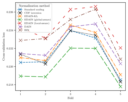
Figure 4: BCE cross-validation loss across different folds in the Amex default prediction dataset.

Our results are reported in Table 2. From the table, it can be inferred that neglecting the preprocessing step deteriorates the performance significantly. Moreover, we observe that the local-aware methods (local-aware EDAIN, BIN, and DAIN) all perform worse than $z$-score normalization. This might be because the data in the dafault prediction dataset is mostly distributed around one central mode, and the local-aware methods discard this information in favour of forming a common representation space. Another possible reason is that the local-aware methods do not preserve the relative ordering between data points $\mathbf{X}^{(i)}$ as per Equation (17), which might be detrimental for these types of datasets. As discussed in the previous section, predictor variables such as credit scores may be present in the dataset, which should only be preprocessed via monotonic transformations. From the results presented in Table 2, we can also conclude that the proposed global-aware version of the EDAIN layer shows superior average performance when compared to all alternative preprocessing methods. Additionally, it must be remarked that most of the variance in the methods’ performance arise from the folds themselves, as seen in Figure 4, and the global-aware EDAIN method consistently shows superior performance across all cross-validation folds when compared to the other methods.

4.3 Financial Forecasting Dataset

For evaluating the proposed methods, we also considered a limit order book (LOB) time series dataset (FI-2010 LOB Ntakaris et al.,, 2018), used as a benchmark dataset in Passalis et al., (2020) and Tran et al., (2021). The data was collected across 10 business days in June 2010 from five Finnish companies (Ntakaris et al.,, 2018), and it was cleaned and features were extracted based on the pipeline of Kercheval and Zhang, (2015). This resulted in $N=453\,975$ vectors of dimensionality $d=144$. The task is predicting whether the mid price will increase, decrease or remain stationary with a prediction horizon of $H=10$ timesteps, where a stock is labelled as stationary if the mid price changes by less than 0.01%. More details on the FI-2010 benchmark dataset can be found in Ntakaris et al., (2018).

For training, we use the anchored cross-validation scheme of Ntakaris et al., (2018). We sequentially increase the size of the training set, starting with a single day and extending it to nine days, while reserving the subsequent day for evaluation in each iteration, obtaining nine different evaluation folds. For evaluating the model performance, we look at the Cohen’s $\kappa$ (Artstein and Poesio,, 2008) and macro-$F_{1}$ score, obtained by averaging class-specific $F_{1}$ scores across the three possible outcomes (increase, decrease or stationary).

Preprocessing method	Cohen’s $\kappa$	Macro-$F_{1}$-score
No preprocessing	$0.0035\pm 0.0049$	$0.2859\pm 0.0228$
$z$-score normalization	$0.2772\pm 0.0550$	$0.5047\pm 0.0403$
CDF inversion	$0.3618\pm 0.0598$	$0.5798\pm 0.0373$
EDAIN-KL	$0.2870\pm 0.0642$	$0.5104\pm 0.0519$
EDAIN (local-aware)	$\mathbf{0.3836\pm 0.0554}$	$\mathbf{0.5946\pm 0.0431}$
EDAIN (global-aware)	$0.2820\pm 0.0706$	$0.5111\pm 0.0648$
BIN	$0.3670\pm 0.0640$	$0.5889\pm 0.0479$
DAIN	$0.3588\pm 0.0506$	$0.5776\pm 0.0341$

Table 3: Experimental results on the FI-2010 LOB dataset, with 95% normal asymptotic confidence intervals $(\mu\pm 1.96\sigma)$ calculated across 9 anchored folds.

We can draw several conclusions from the results reported in Table 3. Firstly, employing some form of preprocessing is essential, as not applying any preprocessing gives $\kappa$ values close to 0, which is what is expected to occur by random guessing. Secondly, applying a local-aware normalization scheme (local-aware EDAIN, BIN and DAIN) greatly improves performance when compared to conventional preprocessing methods such as $z$-score scaling. Our third observation is that the proposed local-aware EDAIN method outperforms both BIN and DAIN on average. Finally, we note that most of the variability in the evaluation metrics arises from the folds themselves, similarly to the default prediction example (cf. Figure 4).

5 CONCLUSION

In this work, we proposed EDAIN, an adaptive data preprocessing layer which can be used to augment any deep neural network architecture that takes multivariate time series as input. EDAIN has four adaptive sublayers (outlier mitigation, shift, scale, and power transform). It also has two versions (local-aware and global-aware), which apply local or global transformations to each time series. Also, we proposed a computationally efficient variant of EDAIN, optimised via the Kullback-Leibler divergence, named EDAIN-KL. The EDAIN layer’s ability to increase the predictive performance of the deep neural network was evaluated on a synthetic dataset, a default prediction dataset, and a financial forecasting dataset. On all datasets considered, either the local-aware or global-aware version of the proposed EDAIN layer consistently demonstrated superior performance.

In Section 4.3, we observed that the local-aware preprocessing methods gave significantly better performance than the global-aware version of EDAIN and $z$-score normalization. However, in Section 4.1 and Section 4.2 the opposite is observed, with the global-aware version of EDAIN demonstrating superior performance and the local-aware methods being outperformed by $z$-score normalization. We hypothesize these differences occur because local-aware methods do not preserve the relative ordering between observations, while the global-aware EDAIN method does. In the financial forecasting dataset, which is highly multi-modal, it appears that the observations’ feature values relative to their mode are more important than their absolute ordering. Such considerations should be taken into account when deciding what adaptive preprocessing method is most suitable for application on new data.

There are several directions for future work. Passalis et al., (2021) observed that the performance improvements from DAIN differed greatly between different deep neural network architectures. Therefore, the effectiveness of EDAIN with other architectures could be further explored as only GRU-based RNNs were considered in this work. Additionally, with the proposed EDAIN method, one has to manually decide whether to apply local-aware or global-aware preprocessing. This drawback could be eliminated by extending the proposed neural layer to apply both schemes to each feature and adaptively learning which version is most suitable. Another common irregularity in real-world data is missing values (Nawi et al.,, 2013; Cao et al.,, 2018). A possible direction would be to extend EDAIN with an adaptive method for treating missing values that makes minimal assumptions on the data generation mechanism (for example, Cao et al.,, 2018).

 

Supplementary Materials
Extended Deep Adaptive Input Normalization for Preprocessing Time Series Data for Neural Network

 

Appendix A MEAN ESTIMATION IN THE OUTLIER MITIGATION LAYER

The $\hat{\bm{\mu}}\in\mathbb{R}^{d}$ vector in Equation (2) is an estimate of the mean of the data, and it is used to ensure the smoothed winsorization operation is centered. When using the local-aware version of the EDAIN layer, it is the mean of the input time series data point:

$$\hat{\bm{\mu}}^{(i)}=\frac{1}{T}\sum_{t=1}^{T}\mathbf{x}_{t}^{(i)}.$$ (26)

In the global-aware version of EDAIN, we consider $\hat{\bm{\mu}}\in\mathbb{R}^{d}$ a fixed quantity, estimating the global mean of the data. As mentioned in the main paper, the $\hat{\bm{\mu}}$ estimate is iteratively computed during training using a cumulative moving average estimate at each forward pass of the sublayer. To do this, we keep track of the current estimated average at forward pass $n=1,2,3,\dots$, denoted $\hat{\bm{\mu}}^{(n)}$, and when we process an input time series $\mathbf{X}^{(i)}$, we apply the update:

$$\hat{\bm{\mu}}^{(n+1)}=\frac{nT\cdot\hat{\bm{\mu}}^{(n)}+\sum^{T}_{t=1}\mathbf{x}_{t}^{(i)}}{(n+1)T}.$$ (27)

We also initialise $\hat{\bm{\mu}}^{(0)}=\mathbf{0}$.

Appendix B EDAIN-KL

The EDAIN-KL layer has a very similar architecture to the EDAIN layer (cf. Section 3 in the main paper), but the unknown parameters are learned via a different optimization procedure. Unlike the EDAIN layer, the EDAIN-KL layer is not attached to the deep neural network during training, but rather training in isolation before training the neural network. This is done by establishing an invertible mapping to transform a standard normal distribution into a distribution that resembles that of our training dataset. Then, after the EDAIN-KL weights have been optimized, we use the layer in reverse to normalize the time series from the training dataset before passing them to the neural network.

B.1 Architecture

Aside from the outlier mitigation sublayer, the EDAIN-KL layer has an identical architecture to the global-aware EDAIN layer. The outlier mitigation transformation has been simplified to ensure its inverse is analytic. Additionally, the layer no longer supports local-aware mode, as this would make the inverse intractable. The EDAIN-KL transformations are:

(outlier mitigation) $$\mathbf{h}_{1}\left(\mathbf{x}^{(i)}_{t}\right)=\bm{\beta}\odot\tanh\left\{(\mathbf{x}^{(i)}_{t}-\hat{\bm{\mu}})\oslash\bm{\beta}\right\}+\hat{\bm{\mu}}$$ (28)

(shift) $$\mathbf{h}_{2}\left(\mathbf{x}^{(i)}_{t}\right)=\mathbf{x}^{(i)}_{t}-\bm{m}$$ (29)

(scale) $$\mathbf{h}_{3}\left(\mathbf{x}^{(i)}_{t}\right)=\mathbf{x}^{(i)}_{t}\oslash\bm{s}$$ (30)

(power transform) $$\mathbf{h}_{4}\left(\mathbf{x}^{(i)}_{t}\right)=\left[f^{\lambda_{1}}_{\textrm{YJ}}\left(x^{(i)}_{t,1}\right),\quad\cdots,\quad f^{\lambda_{d}}_{\textrm{YJ}}\left(x^{(i)}_{t,d}\right)\right],$$ (31)

where $f^{\lambda_{i}}_{\textrm{YJ}}(\cdot)$ is defined in the main paper in Equation (3).

B.2 Optimisation through Kullback-Leibler divergence

The optimisation approach used to train the EDAIN-KL method is inspired by normalizing flows (see, for example, Kobyzev et al.,, 2021). Before describing the approach, we provide a brief overview of related notation and some background on the concept behind normalizing flows. After this, we describe how the EDAIN-KL layer itself can be treated as an invertible bijector to fit into the normalizing flow framework. In doing so, we derive analytic and differentiable expressions for certain terms related to the EDAIN-KL layer.

B.2.1 Brief background on normalizing flow

The idea behind normalizing flows is taking a simple random variable, such as a standard Gaussian, and transforming it into a more complicated distribution, for example, one that resembles the distribution of a given real-world dataset. Consider a random variable $\mathbf{Z}\in\mathbb{R}^{d}$ with a known and analytic expression for its PDF $p_{\mathbf{z}}:\mathbb{R}^{d}\rightarrow{\mathbb{R}}$. We refer to $\mathbf{Z}$ as the base distribution. We then define a parametrised invertible function $\mathbf{g}_{\bm{\theta}}:\mathbb{R}^{d}\rightarrow{\mathbb{R}^{d}}$, also known as a bijector, and use this to transform the base distribution into a new probability distribution: $\mathbf{Y}=\mathbf{g}_{\bm{\theta}}(\mathbf{Z})$. By increasing the complexity of the bijector $\mathbf{g}_{\bm{\theta}}$ (for example, by using a deep neural network), the transformed distribution $\mathbf{Y}$ can grow arbitrarily complex as well. The PDF of the transformed distribution can then be computed using the change of variable formula (Kobyzev et al.,, 2021), where

$$p_{\mathbf{Y}}(\mathbf{y})=p_{\mathbf{Z}}(\mathbf{g}_{\bm{\theta}}^{-1}\left(\mathbf{y}\right))\cdot\left|\det\mathbf{J}_{\mathbf{Y}\rightarrow{\mathbf{Z}}}\left(\mathbf{y}\right)\right|=p_{\mathbf{Z}}(\mathbf{g}_{\bm{\theta}}^{-1}\left(\mathbf{y}\right))\cdot\left|\det\mathbf{J}_{\mathbf{Z}\rightarrow{\mathbf{Y}}}\left(\mathbf{g}^{-1}_{\bm{\theta}}(\mathbf{y})\right)\right|^{-1},$$ (32)

and where $\mathbf{J}_{\mathbf{Z}\rightarrow{\mathbf{Y}}}$ is the Jacobian matrix for the forward mapping $\mathbf{g}_{\bm{\theta}}:\mathbf{z}\mapsto\mathbf{y}$. Taking logs on both sides of Equation (32), it follows that

$$\log p_{\mathbf{Y}}(\mathbf{y})=\log p_{\mathbf{Z}}(\mathbf{g}_{\bm{\theta}}^{-1}\left(\mathbf{y}\right))-\log\left|\det\mathbf{J}_{\mathbf{Z}\rightarrow{\mathbf{Y}}}\left(\mathbf{g}_{\bm{\theta}}^{-1}\left(\mathbf{y}\right)\right)\right|.$$ (33)

One common application of normalizing flows is density estimation (Kobyzev et al.,, 2021). Given a dataset $\mathcal{D}=\{\mathbf{y}^{(i)}\}_{i=1}^{N}$ with samples from some unknown, complicated distribution, we want to estimate its PDF. This can be done with likelihood-based estimation, where we assume the data points $\mathbf{y}^{(1)},\mathbf{y}^{(2)},\dots,\mathbf{y}^{(N)}$ come from, say, the parametrised distribution $\mathbf{Y}=\mathbf{g}_{\bm{\theta}}(\mathbf{Z})$ and we optimise $\bm{\theta}$ to maximise the data log-likelihood,

$$\log p(\mathcal{D}|\bm{\theta})=\sum_{i=1}^{N}\log p_{\mathbf{Y}}(\mathbf{y}^{(i)}|\bm{\theta})\stackrel{{\scriptstyle\eqref{eq:logDetJac}}}{{=}}\sum^{N}_{i=1}\log p_{\mathbf{Z}}\left(\mathbf{g}_{\bm{\theta}}^{-1}\left(\mathbf{y}^{(i)}\right)\right)-\log\left|\det\mathbf{J}_{\mathbf{Z}\rightarrow{\mathbf{Y}}}\left(\mathbf{g}_{\bm{\theta}}^{-1}\left(\mathbf{y}^{(i)}\right)\right)\right|.$$ (34)

It can be shown that this is equivalent to minimising the KL-divergence between the empirical distribution $\mathcal{D}$ and the transformed distribution $\mathbf{Y}=\mathbf{g}_{\bm{\theta}}(\mathbf{Z})$ (see, for example, Kobyzev et al.,, 2021):

$$\operatorname*{argmax}_{\bm{\theta}}\log p(\mathcal{D}|\bm{\theta}) =\operatorname*{argmax}_{\bm{\theta}}\sum_{i=1}^{N}\log p_{\mathbf{Y}}\left(\mathbf{y}^{(i)}\big{|}\bm{\theta}\right)=\operatorname*{argmin}_{\bm{\theta}}\mathrm{KL}\left\{\mathcal{D}\ ||\ \mathbf{g}_{\bm{\theta}}(\mathbf{Z})\right\}.$$ (35)

When training a normalizing flow model, we want to find the parameter values $\bm{\theta}$ that minimize the above KL-divergence. This is done using back-propagation, where the criterion $\mathcal{L}$ is set to be the negation of Equation (34). That is, the loss becomes the negative log likelihood of a batch of samples from the training dataset. To perform optimisation with this criterion, we need to compute all the terms in Equation (34), and this expression needs to be differentiable because the back-propagation algorithm uses the gradient of the loss with respect to the input data. We therefore need to find

1. an analytic and differentiable expression for the inverse transformation $\mathbf{g}_{\bm{\theta}}^{-1}\left(\cdot\right)$,

2. an analytic and differentiable expression for the PDF of the base distribution $p_{\mathbf{Z}}(\cdot)$, and

3. an analytic and differentiable expression for the log determinant of the Jacobian matrix for $\mathbf{g}_{\bm{\theta}}$, that is, $\log\left|\det\mathbf{J}_{\mathbf{Z}\rightarrow{\mathbf{Y}}}\right|$.

We will derive these three components for our EDAIN-KL layer in the next section, where we extensively use the following proposition (Kobyzev et al.,, 2021, see, for example,):

Proposition B.1.

Let $\mathbf{g}_{1},\dots,\mathbf{g}_{n}:\mathbb{R}^{d}\rightarrow{\mathbb{R}^{d}}$ all be bijective functions, and consider the composition of these functions, $\mathbf{g}=\mathbf{g}_{n}\circ\mathbf{g}_{n-1}\cdots\circ\mathbf{g}_{1}$. Then, $\mathbf{g}$ is a bijective function with inverse

$$\mathbf{g}^{-1}=\mathbf{g}_{1}^{-1}\circ\cdots\circ\mathbf{g}_{n-1}^{-1}\circ\mathbf{g}_{n}^{-1},$$ (36)

and the log of the absolute value of the determinant of the Jacobian is given by

$$\log\left|\det\mathbf{J}_{\mathbf{g}^{-1}}(\cdot)\right|=\sum_{i=1}^{N}\log\left|\det\mathbf{J}_{\mathbf{g}_{i}^{-1}}(\cdot)\right|.$$ (37)

B.2.2 Application to EDAIN-KL

Like with the EDAIN layer, we want to compose the outlier mitigation, shift, scale and power transform transformations into one operation, which we do by defining

$$\mathbf{g}_{\bm{\theta}}=\mathbf{h}_{1}^{-1}\circ\mathbf{h}_{2}^{-1}\circ\mathbf{h}_{3}^{-1}\circ\mathbf{h}_{4}^{-1},$$ (38)

where $\bm{\theta}=(\bm{\beta},\bm{m},\bm{s},\bm{\lambda})$ are the unknown parameters and $\mathbf{h}_{1},\dots,\mathbf{h}_{4}$ are defined in Equations (28), (29), (30) and (31), respectively. Notice how we apply all the operations in reverse order, compared to the EDAIN layer. This is because we will use $\mathbf{g}_{\bm{\theta}}$ to transform our base distribution $\mathbf{Z}$ into a distribution that resembles the training dataset, $\mathcal{D}$, not the other way around. Then, to normalize the dataset after fitting the EDAIN-KL layer, we apply

$$\mathbf{g}_{\bm{\theta}}^{-1}=\mathbf{h}_{4}\circ\mathbf{h}_{3}\circ\mathbf{h}_{2}\circ\mathbf{h}_{1}$$ (39)

to each time series data point, similar to the EDAIN layer. It can be shown that all the transformations defined in Equations (28), (29), (30) and (31) are invertible, of which a proof is given in the next subsection. Using Lemma B.1, it thus follows that $\mathbf{g}_{\bm{\theta}}$, as defined in Equation (38), is bijective and that its inverse is given by Equation (39). Since we already have analytic and differentiable expressions for $\mathbf{h}_{1}$, $\mathbf{h}_{2}$, $\mathbf{h}_{3}$ and $\mathbf{h}_{4}$ from Equations (28), (29), (30) and (31), it follows that $\mathbf{g}_{\bm{\theta}}^{-1}$, as defined in Equation (39), is an analytic and differentiable expression, so part (i) is satisfied.

We now move onto deciding what our base distribution should be. As we validated experimentally in Section 4.1 of the main paper, Gaussianizing the input data could increase the performance of deep neural networks (depending on the data generating process). Therefore, we let the base distribution be the standard multivariate Gaussian distribution

$$\mathbf{Z}\sim\mathcal{N}(\mathbf{0}_{d},\mathbf{I}_{d}),$$ (40)

whose PDF $p_{\mathbf{Z}}(\cdot)$ has an analytic and differentiable expression, so part $(\textrm{ii})$ is satisfied.

In the next subsection, we will derive part (iii): an analytic and differentiable expression for the log of the determinant of the Jacobian matrix of $\mathbf{g}_{\bm{\theta}}$, $\log\left|\det\mathbf{J}_{\mathbf{Z}\rightarrow{\mathbf{Y}}}\right|$. Once that is done, parts (i), (ii) and (iii) are satisfied, so $\bm{\theta}$ can be optimised using back-propagation using the negation of Equation (34) as the objective. In other words, we can optimise $\bm{\theta}$ to maximise the likelihood of the training data under the assumption that it comes from the distribution $\mathbf{Y}=\mathbf{g}_{\bm{\theta}}(\mathbf{Z})$. This is desirable, as if we can achieve a high data likelihood, the samples $\mathcal{D}=\{\mathbf{y}^{(i)}\}_{i=1,2,\dots,N}$ will more closely resemble a standard normal distribution after being transformed by $\mathbf{g}_{\bm{\theta}}^{-1}$. Also recall that multivariate time series data are considered in this work, so the “$\mathbf{y}$”-samples will be of the form $\mathbf{X}^{(i)}\in\mathbb{R}^{d\times T}$.

B.2.3 Derivation of the inverse log determinant of the Jacobian

Recall that the EDAIN-KL architecture is a bijector composed of four other bijective functions. Using the result in Equation (B.1), we get

$$\log\left|\det\mathbf{J}_{\mathbf{Z}\rightarrow{\mathbf{Y}}}(\cdot)\right|=\sum^{4}_{i=1}\log\left|\det\mathbf{J}_{\mathbf{h}_{i}^{-1}}(\cdot)\right|.$$ (41)

Considering the transformations in Equations (28), (29), (30) and (31), we notice that all the transformations happen element-wise, so for $i\in\{1,2,3,4\}$, we have $\left[\frac{\partial\mathbf{h}_{i}^{-1}(\mathbf{x})}{\partial x_{k}}\right]_{j}=0$ for $k\neq j$. Therefore, the Jacobians are diagonal matrices, implying that the determinant is the product of the diagonal entries, giving

$$\log\left|\det\mathbf{J}_{\mathbf{Z}\rightarrow{\mathbf{Y}}}(\mathbf{x})\right|=\sum^{4}_{i=1}\log\left|\prod_{j=1}^{d}\left[\frac{\partial\mathbf{h}_{i}^{-1}(\mathbf{x})}{\partial x_{j}}\right]_{j}\right|=\sum^{4}_{i=1}\sum_{j=1}^{d}\log\left|\frac{\partial h_{i}^{-1}\left(x_{j};\theta_{j}^{(i)}\right)}{\partial x_{j}}\right|,$$ (42)

where in the last step we used the fact that $h_{1},h_{2},h_{3}$ and $h_{4}$ are applied element-wise to introduce the notation $h_{i}(x_{j};\theta^{(i)}_{j})$. This means, applying $\mathbf{h}_{i}$ to some vector where the $j$th element is $x_{j}$, and the corresponding $j$th transformation parameter takes the value $\theta^{(i)}_{j}$. For example, for the scale function $\mathbf{h}_{3}(\mathbf{x})=\mathbf{x}\oslash\bm{s}$, we have $h_{3}(x_{j};\lambda_{j})=\frac{x_{j}}{s_{j}}$. From Equation (42), we know that we only need to derive the derivatives for the element-wise inverses, which we will now do for each of the four transformations, also demonstrating that each transformation is bijective.

Shift.

We first consider $h_{2}(x_{j};m_{j})=x_{j}-m_{j}$. Its inverse is $h_{2}^{-1}(z_{j};m_{j})=z_{j}+m_{j}$, and it follows that

$$\log\left|\frac{\partial h_{2}^{-1}(z_{j};m_{j})}{\partial z_{j}}\right|=\log 1=0.$$ (43)

Scale.

We now consider $h_{3}(x_{j};s_{j})=\frac{x_{j}}{s_{j}}$, whose inverse is $h_{3}^{-1}(x_{j};s_{j})={z_{j}}{s_{j}}$. It follows that

$$\log\left|\frac{\partial h_{3}^{-1}(z_{j};s_{j})}{\partial z_{j}}\right|=\log\left|{s_{j}}\right|.$$ (44)

Outlier mitigation.

We now consider $h_{1}(x_{j};\beta_{j})=\beta_{j}\tanh\left\{\frac{(x_{j}-\hat{\mu}_{j})}{\beta_{j}}\right\}+\hat{\mu}_{j}$. Its inverse is

$$h_{1}^{-1}(z_{j};\beta_{j})=\beta\tanh^{-1}\left\{\frac{z_{j}-\hat{\mu}_{j}}{\beta_{j}}\right\}+\hat{\mu}_{j}.$$ (45)

It follows that

$$\log\left|\frac{\partial h_{1}^{-1}(z_{j};\beta_{j})}{\partial z_{j}}\right|=\log\left|\frac{1}{1-\left(\frac{z_{j}-\hat{\mu}_{j}}{\beta_{j}}\right)^{2}}\right|=-\log\left|1-\left(\frac{z_{j}-\hat{\mu}_{j}}{\beta_{j}}\right)^{2}\right|.$$ (46)

Power transform.

By considering Equation (31), it can be shown that for fixed $\lambda$, negative inputs are always mapped to negative values and vice versa, which makes the Yeo-Johnson transformation invertible. Additionally, in $\mathbf{h}_{4}(\cdot)$ the Yeo-Johnson transformation is applied element-wise, so we get

$$\mathbf{h}_{4}^{-1}(\mathbf{z})=\left[\left[f_{\textrm{YJ}}^{\lambda_{1}}\right]^{-1}\bigg{(}z_{1}\bigg{)},\quad\left[f_{\textrm{YJ}}^{\lambda_{2}}\right]^{-1}\bigg{(}z_{2}\bigg{)},\quad\cdots,\quad\left[f_{\textrm{YJ}}^{\lambda_{d}}\right]^{-1}\bigg{(}z_{d}\bigg{)}\right],$$ (47)

where it can be shown that the inverse Yeo-Johnson transformation for a single element is given by

$$\left[f_{\textrm{YJ}}^{\lambda}\right]^{-1}\bigg{(}z\bigg{)}=\left\{\begin{array}[]{ll}(z\lambda+1)^{1/\lambda}-1,&\textrm{if }\lambda\neq 0,z\geq 0;\\ e^{z}-1,&\textrm{if }\lambda=0,z\geq 0;\\ 1-\left\{1-z(2-\lambda)\right\}^{1/(2-\lambda)},&\textrm{if }\lambda\neq 2,z<0;\\ 1-e^{-z},&\textrm{if }\lambda=2,z<0.\end{array}\right.$$ (48)

The derivative with respect to $z$ then becomes

$$\frac{\partial\left[f_{\textrm{YJ}}^{\lambda}\right]^{-1}(z)}{\partial z}=\left\{\begin{array}[]{ll}(z\lambda+1)^{(1-\lambda)/\lambda},&\textrm{if }\lambda\neq 0,z\geq 0;\\ e^{z},&\textrm{if }\lambda=0,z\geq 0;\\ \left\{1-z(2-\lambda)\right\}^{(\lambda-1)/(2-\lambda)},&\textrm{if }\lambda\neq 2,z<0;\\ e^{-z},&\textrm{if }\lambda=2,z<0.\end{array}\right.$$ (49)

It follows that

$$\log\left|\frac{\partial\left[f_{\textrm{YJ}}^{\lambda}\right]^{-1}(z)}{\partial z}\right|=\left\{\begin{array}[]{ll}\frac{1-\lambda}{\lambda}\log(z\lambda+1),&\textrm{if }\lambda\neq 0,z\geq 0;\\ z,&\textrm{if }\lambda=0,z\geq 0;\\ \frac{\lambda-1}{2-\lambda}\log\left\{1-z(2-\lambda)\right\},&\textrm{if }\lambda\neq 2,z<0;\\ -z,&\textrm{if }\lambda=2,z<0,\end{array}\right.$$ (50)

which we use as the expression for $\log\left|\frac{\partial h_{4}^{-1}\left(z_{j};\lambda_{j}\right)}{\partial z_{j}}\right|$ for $z=z_{1},\dots,z_{d}$.

Combining these expressions, we get an analytical and differentiable form for $\log\left|\det\mathbf{J}_{\mathbf{Z}\rightarrow{\mathbf{Y}}}(\mathbf{x})\right|$, as required.

Appendix C EXPERIMENTAL EVALUATION DETAILS ON MODELS AND TRAINING

In this section, we provide details on the specific RNN model architectures used for evaluation in Section 4 of the main paper. We then cover the optimization procedures used for the three datasets, including details such as number of training epochs, learning rates and choice of optimizers. Then, we list the learning rate modifiers used for the different adaptive preprocessing layers, and explain how these were selected.

C.1 Deep Neural Network Model Architectures

Synthetic dataset.

The GRU RNN architecture consisted of two GRU cells with a dimensionality of 32 and dropout layer with dropout probability $p=\frac{1}{5}$ between these cells. This was followed by a linear feed-forward neural network with 3 fully-connected layers, separated by ReLU activation functions, of 64, 32 and 1 units, respectively. The output was then passed through a sigmoid layer to produce a probability $p\in(0,1)$.

Default prediction dataset.

We use a RNN sequence model, with a classifier head, for all our experiments with the default prediction dataset. It consists of two stacked GRU RNN cells, both with a hidden dimensionality of 128. Between these cells, there is a dropout layer with the dropout probability of $p=20\%$. For the 11 categorical features present in the dataset, we pass these through separate embedding layers, each with a dimensionality of 4. The outputs of the embedding layers are then combined with the output of the last GRU cell, after it has processed the numeric columns, and the result is passed to the linear classifier head. The classifier head is a conventional linear neural network consisting of 2 linear layers with 128 and 64 units each, respectively, and separated by ReLU activation functions. The output is then fed through a linear layer with a single output neuron, followed by a sigmoid activation function to constrain the output to be a probability in the range $(0,1)$. The described architecture was chosen because it worked well in our initial experiments.

Financial forecasting dataset.

For the FI-2010 LOB dataset, we use a similar GRU RNN model as with the Amex dataset, but change the architecture slightly to match the RNN model used by Passalis et al., (2020). This was done to make the comparison between the proposed EDAIN method and their DAIN method more fair, seeing as they also used the LOB dataset to evaluate DAIN. Instead of using two stacked GRU cells, we use one with 256 units. We also do not need any embedding layers because all the predictor variables are numeric. The classifier head that follows the GRU cells consists of one linear layer with 512 units, followed by a ReLU layer and a dropout layer with a dropout probability of $p=0.5$. The output layer is a linear layer with 3 units, as we are classifying the multivariate time series into one of three classes, $\mathcal{C}=\{\textrm{decrease},\textrm{stationary},\textrm{increase}\}$. These outputs are then passed to a softmax activation function such that the output is a probability distribution over the three classes and sums to 1: $\left[\textrm{softmax}(\mathbf{y})\right]_{j}={e^{y_{j}}}/{\sum^{k}_{i=1}e^{y_{i}}},\ j=1,2,\dots,k$. In our case, we have $k=3$.

C.2 Optimization Procedures

Synthetic dataset.

For the synthetic dataset, all the $N_{\mathcal{D}}$ generated datasets were separated into 80%-20% train-validation splits, and the metrics reported in Table 1 of the main paper are based on metrics computed for model performance on the validation splits. The training was done using the Adam optimizer proposed by Kingma and Ba, (2015) using a base learning rate of $\eta=10^{-3}$ and the model was trained for 30 epochs. We also used a multi-step learning rate scheduler with decay $\gamma=\frac{1}{10}$ at the 4th and 7th epoch. Additionally, an early stopper was used on the validation loss with a patience of 5. The model was trained using binary cross-entropy loss, and the batch size was 128.

Default prediction dataset.

To evaluate the different preprocessing methods on this dataset, we perform 5-fold cross validation, which gives evaluation metrics for five different 20% validation splits. For training, we used a batch size of 1024. This was chosen to give a good trade-off between the time required to train the model and predictive performance. This model was also optimised with the Adam optimizer proposed by Kingma and Ba, (2015). The learning rate was also set to $\eta=10^{-3}$ after testing what learning rate from the set $H=\{10^{-1},10^{-2},10^{-3},10^{-4}\}$ gave the most stable convergence. The momentum parameters $\beta_{1}$ and $\beta_{2}$ were set to their default values according to the PyTorch implementation of the optimizer (Paszke et al.,, 2019). We also used a multi-step learning rate scheduler, with the step size set to $\gamma=\frac{1}{10}$. For the milestones (corresponding to the epoch indices at which the learning rate changes), we first tuned the first step based on observing the learning rate curve during training; then, we set the step epoch to ensure the performance did not change too rapidly. This was done until we got milestones at 4 and 7. We also used an early stopper based on the validation loss, with the patience set to $p_{\textrm{patience}}=5$ as this worked well in our initial experiments. The maximum number of training epochs was set to 40.

Financial forecasting dataset.

As discussed in the main paper, we use an anchored cross-validation scheme for training, which gives 9 different train-validation splits based on the 10 days of training data available. The targets are ternary labels $y_{1},y_{2},\dots,y_{N}\in\{0,1,2\}$, denoting whether the mid-price decreased, remained stationary, or increased, and the output of the model is probability vectors $\mathbf{p}_{1},\mathbf{p}_{2},\dots,\mathbf{p}_{N}\in(0,1)^{3}$. For optimising the model parameters, we use the cross-entropy loss function, defined as

$$\mathcal{L}(\mathbf{p}_{i},y_{i})=-\sum^{2}_{c=0}\mathbb{I}_{\{y_{i}=c\}}\log\left(p_{i,c}\right),$$ (51)

where $p_{i,c}$ denotes the predicted probability of class $c$ for the $i$th input sample. We used a batch size of 128, and used the RMSProp optimizer proposed by Hinton and Tieleman, (2012) to be consistent with the experiments by Passalis et al., (2020). The base learning rate was set to $\eta=10^{-4}$. No learning rate scheduler nor early stoppers were used: this was done to best reproduce the methodology used by Passalis et al., (2020). Despite not using any early stoppers, all the metrics were computed based on the model state at the epoch where the validation loss was lowest. This was because the generalization performance started to decline in the middle of training in most cases. At each training fold, the model was trained for 20 epochs.

C.3 Sublayer Learning Rate Modifiers

C.3.1 Synthetic dataset

For the synthetic data, we use the learning rate modifier $\eta^{\prime}=10^{-1}$ for all sublayers of all adaptive preprocessing layers (BIN, DAIN, and EDAIN), while as mentioned in Section C.2, the base learning rate is $\eta=10^{-3}$.

C.3.2 Default prediction dataset

The BIN method proposed by Tran et al., (2021) and the DAIN method proposed by Passalis et al., (2020) have both never been applied to the American Express default prediction dataset before, so their hyperparameters are tuned for this dataset. We also tune the two versions of EDAIN. For all these experiments, we run a grid-search with different combinations of the hyperparameters, specifically the learning rate modifiers, using the validation loss from training a single model for 10 epochs on a 80%-20% split of the training dataset. We then pick the combination giving the lowest validation loss. We now provide details on the grids used for each of the different preprocessing layers, and what learning rate modifiers gave the best performance.

BIN.

We used the grids:

$H_{\beta}=\{10,1,10^{-1},10^{-2},10^{-6}\}$,

$H_{\gamma}=\{10,1,10^{-1},10^{-2},10^{-6}\}$, and

$H_{\lambda}=\{10,1,10^{-1},10^{-2},10^{-6}\}$.

The combination giving the lowest average cross-validation loss was found to be $\eta_{\beta}=10$, $\eta_{\gamma}=1$, and $\eta_{\lambda}=10^{-6}$, giving 0.2234.

DAIN.

We used the grids:

$H_{\textrm{shift}}=\{10,1,10^{-1},10^{-2},10^{-3},10^{-4}\}$ and

$H_{\textrm{scale}}=\{10,1,10^{-1},10^{-2},10^{-3},10^{-4}\}$.

The combination giving the lowest average cross-validation loss was found to be $\eta_{\textrm{shift}}=1$ and $\eta_{\textrm{scale}}=1$, giving $0.2216$.

Global-aware EDAIN.

We used the grids:

$H_{\textrm{scale}}=H_{\textrm{shift}}=H_{\textrm{outlier}}=H_{\textrm{pow}}=\{100,10,1,10^{-1},10^{-2},10^{-3}\}$.

The combination giving the lowest average cross-validation loss was found to be $\eta_{\textrm{shift}}=10^{-2}$, $\eta_{\textrm{scale}}=10^{-2}$, $\eta_{\textrm{outlier}}=10^{2}$, and $\eta_{\textrm{pow}}=10$, giving $0.2190$.

Local-aware EDAIN.

We used the grids:

$H_{\textrm{scale}}=H_{\textrm{shift}}=\{1,10^{-1},10^{-2}\}$ and $H_{\textrm{outlier}}=H_{\textrm{pow}}=\{10,1,10^{-1},10^{-2},10^{-3}\}$.

The combination giving the lowest average cross-validation loss was found to be $\eta_{\textrm{shift}}=1$, $\eta_{\textrm{scale}}=1$, $\eta_{\textrm{outlier}}=10$, and $\eta_{\textrm{pow}}=10$, giving $0.2243$.

EDAIN-KL.

Note that due to numerical gradient errors in the power transform layers occurring for some choices of power transform learning rates, the values considered are all low to avoid these errors. We used the grids

$H_{\textrm{outlier}}=\{100,10,1,10^{-1},10^{-2},10^{-3}\}$,

$H_{\textrm{scale}}=\{100,10,1,10^{-1},10^{-2},10^{-3}\}$,

$H_{\textrm{shift}}=\{100,10,1,10^{-1},10^{-2},10^{-3}\}$, and

$H_{\textrm{pow}}=\{10^{-7}\}$

The combination giving the lowest average cross-validation loss was found to be $\eta_{\textrm{shift}}=10$, $\eta_{\textrm{scale}}=10$, $\eta_{\textrm{outlier}}=10^{2}$, and $\eta_{\textrm{pow}}=10^{-7}$, giving $0.2208$.

C.3.3 Financial forecasting dataset

The BIN method proposed by Tran et al., (2021) and the DAIN method proposed by Passalis et al., (2020) have already been applied to the LOB dataset before, but only DAIN has been applied with the specific GRU RNN architecture we are using. Therefore, the learning rate modifiers found by Passalis et al., (2020) will be used as-is ($\eta_{\textrm{shift}}=10^{-2},\eta_{\textrm{scale}}=10^{-8}$), and the learning rate modifiers for the remaining methods will be tuned. The details of this are presented here. For all the learning rate tuning experiments, we used the first day of data from the FI-2010 LOB for training and the data from the second day for validation. We then pick the combination giving the highest validation Cohen’s $\kappa$-metric.

BIN.

We used the grids:

$H_{\beta}=\{10,1,10^{-1},10^{-2},10^{-6},10^{-8}\}$,

$H_{\gamma}=\{10,1,10^{-1},10^{-2},10^{-6},10^{-8}\}$, and

$H_{\lambda}=\{10,1,10^{-1},10^{-2},10^{-6},10^{-8}\}$.

The combination giving the highest $\kappa$ was found to be $\eta_{\beta}=1$, $\eta_{\gamma}=10^{-8}$, and $\eta_{\lambda}=10^{-1}$, giving $\kappa=0.3287$.

Global-aware EDAIN.

We used the grids:

$H_{\textrm{scale}}=H_{\textrm{shift}}=H_{\textrm{outlier}}=H_{\textrm{pow}}=\{10,10^{-1},10^{-3},10^{-6}\}$.

The combination giving the highest $\kappa$ was found to be $\eta_{\textrm{shift}}=10$, $\eta_{\textrm{scale}}=10$, $\eta_{\textrm{outlier}}=10^{-6}$, and $\eta_{\textrm{pow}}=10^{-3}$, giving $\kappa=0.2788$.

Local-aware EDAIN.

We used the grids:

$H_{\textrm{scale}}=\{10^{-1},10^{-4},10^{-8}\}$,

$H_{\textrm{shift}}=\{10^{-1},10^{-2}\}$,

$H_{\textrm{outlier}}=\{10,1,10^{-1},10^{-2},10^{-3},10^{-5},10^{-7}\}$, and

$H_{\textrm{pow}}=\{10,1,10^{-1},10^{-2},10^{-3},10^{-5},10^{-7}\}$.

The combination giving the highest $\kappa$ was found to be $\eta_{\textrm{shift}}=10^{-2}$, $\eta_{\textrm{scale}}=10^{-4}$, $\eta_{\textrm{outlier}}=10$, and $\eta_{\textrm{pow}}=10$, giving $\kappa=0.3859$.

EDAIN-KL.

$H_{\textrm{scale}}=\{10^{-1},10^{-4},10^{-7}\}$,

$H_{\textrm{shift}}=\{10^{-1},10^{-2}\}$,

$H_{\textrm{outlier}}=\{10,1,10^{-1},10^{-2},10^{-3},10^{-5},10^{-7}\}$, and

$H_{\textrm{pow}}=\{10^{-2},10^{-3},10^{-5},10^{-7}\}$.

The combination giving the highest $\kappa$ was found to be $\eta_{\textrm{shift}}=10^{-2}$, $\eta_{\textrm{scale}}=10^{-4}$, $\eta_{\textrm{outlier}}=10$, and $\eta_{\textrm{pow}}=10^{-3}$, giving $\kappa=0.2757$.

C.4 Description of Computing Infrastructure

All experiments were run on a Asus ESC8000 G4 server with the following specifications:

• two 16-core CPUs of model Intel(R) Xeon(R) Gold 6242 CPU @ 2.80GHz,

• 896 GiB of system memory,

• eight GPUs of model NVIDIA GeForce RTX 3090, each with $24\,576~{}\textrm{MiB}$ of video memory (VRAM).

Appendix D SYNTHETIC DATA GENERATION ALGORITHM

To help with designing preprocessing methods that can increase the predictive performance as much as possible, we propose a synthetic data generation algorithm that gives full control over how the variables are distributed, through only needing to specify an unnormalized PDF function for each variable. This allows synthesizing data with distributions having the same irregularities as that seen in real-world data. Additionally, the covariance structure of the generated data can be configured to resemble that of real-world multivariate time series, which most often have significant correlation between the predictor variables. Along with each time series generated, we also create a response $y\in\{0,1\}$ that is based on the covariates, allowing for supervised classification tasks.

The main input to the data generation procedure is the time series length, $T\in\mathbb{N}$, and the number of features, $d\in\mathbb{N}$. For each predictor variable $j=1,2,\dots,d$, we also specify an unnormalized PDF, $f_{j}:\mathbb{R}\rightarrow{\mathbb{R}}_{+}$. The data generation procedure then generates a multivariate time series covariate $\mathbf{X}\in\mathbb{R}^{d\times T}$ and a corresponding response $y\in\{0,1\}$ in three steps. Note that this procedure is repeated $N$ times to, say, generate a dataset of $N$ time series. An overview of the the three steps of the data generation algorithm is shown in Figure 5. Each row in the three matrices corresponds to one predictor variable and the column specifies the timestep.

$$\qquad\qquad\qquad\bigg{\downarrow}\quad U_{j,t}=\Phi_{\mathcal{N}}\left(N_{j,t}\big{/}\sqrt{\Sigma^{\prime}_{jT+t,jT+t}}\right)$$

$$\qquad\qquad\qquad\bigg{\downarrow}\quad X_{j,t}=\widehat{F^{-1}_{j}}\left(U_{j,t}\right)\qquad\forall t=1,2,\dots,T$$

Figure 5: High-level overview of the proposed synthetic data generation algorithm.

In the first step in Equation (52), we generate Gaussian random variables that have a similar covariance structure to a multivariate time series. This ensures the covariates’ covariance more closely resemble that of real-world sequence data. In the second step, shown in Equation (53), we convert the Gaussian random variables into uniform random variables using the inverse normal CDF, after standardizing each variable. In this step, we also form the response through a linear combination of unknown parameters $\bm{\beta}$ and the uniform random variables. This ensures there is some mutual information between the response and the covariates that are generated in the final step. In step 3, shown in Equation (54), we form the final covariates using the provided PDFs $f_{1},f_{2},\dots,f_{d}$. This is done by estimating each PDF’s inverse CDF using numerical methods, and transforming the uniform random variables with these. This makes the samples come from a distribution matching that of the provided PDFs. Moreover, in Equations (52), (53), and (54) we use random variable notation for each of the steps, but in practice, all the transformations are applied on samples from these.

D.1 Step 1: Generating random variables with a time series covariance structure

One approach to reproducing the covariance structure of a multivariate time series is to assume that each of the $d$ individual time series follow a moving average model, which is a common type of theoretical time series (Hyndman and Athanasopoulos,, 2018). With this model, the covariate at timestep $t$ takes the form

$$X_{t}=c-\sum^{q}_{j=0}\theta_{j}\epsilon_{t-j},$$ (55)

where $c\in\mathbb{R}$ is a constant, $\epsilon_{0},\epsilon_{1},\dots$ are uncorrelated random variables with zero mean and finite variance $\sigma_{\epsilon}\in\mathbb{R}$. Also, $\theta_{0}=-1$ and $\theta_{1},\dots,\theta_{q}\in(-1,1)$ are the unknown parameters. Under this model, Hyndman and Athanasopoulos, (2018) state that the covariance between a sample from timestep $t$ and a sample from $\tau\in\mathbb{Z}$ timesteps into the future is

$$s_{\tau}=\textrm{cov}\{X_{t},X_{t+\tau}\}=\sigma_{\epsilon}^{2}\sum^{q-\tau}_{j=0}\theta_{j}\theta_{j+\tau}.$$ (56)

We will not be generating our covariates using the model in Equation (55) as this would make it infeasible to get samples that are distributed according to arbitrary PDFs. However, we can use the covariance formula from Equation (56) to set the covariance between each pair of variables generated. To do this, we first specify the parameters $q$, $\sigma_{\epsilon}$, and $\theta_{0},\dots,\theta_{q}$ for each of the $d$ predictor variables. Then, we stack the Gaussian random variables $N_{1,1},N_{1,2},\dots,N_{2,1},N_{2,2},\dots,N_{d,T}$ in Equation (52) row-wise so that they form a $dT$-long vector. Let $\Sigma\in\mathbb{R}^{dT\times dT}$ denote the covariance matrix of this $dT$-long Gaussian multivariate random variable. While still thinking of each $T$-length row as its own univariate time series, we fill out the entries in $\Sigma$ based on Equation (56), using the parameters specified for each of the $d$ time series. The remaining entries of $\Sigma$ are randomly initialised with samples from $\mathcal{N}(\mu=0,\sigma=\sigma_{\textrm{cor}})$, where $\sigma_{\textrm{cor}}$ is a hyperparameter for the data synthesis, with the motivation being to create some cross-dependence between each time series. In order to use $\Sigma$ as a valid covariance matrix for sampling from the $dT$-dimensional multivariate normal distribution, it needs to be symmetric positive semi-definite. The $\Sigma$ matrix we have constructed so far has no guarantee of satisfying this. Therefore, we use the algorithm proposed by Higham, (1988) to find the symmetric positive semi-definite matrix $\Sigma^{\prime}\in\mathbb{R}^{dT\times dT}$ that is closest to $\Sigma$ according to the Frobenius norm. More details on this procedure can be found in Higham, (1988). After this, we generate a $dT$-dimensional sample $\mathbf{N}\sim\mathcal{N}(\mathbf{0},\Sigma^{\prime})$ and imagine “unrolling” this into a $d\times T$ matrix where we have a $T$-timestep-long time series in each row, just as in Equation (52).

D.2 Step 2: Forming the response

Before forming the response $y$, we need to convert the Gaussian random variables generated in step 1 into uniform random variables. By the probability integral transform, if a normal random variable is passed through its inverse CDF-function, a uniform random variable is obtained. Therefore, we do this for each of the normal random variables, as shown in the transition between Equation (52) and Equation (53), giving $d$ time series of uniform random variables, each of length $T$.

To form the response, we randomly sample a noise term $\zeta\sim\mathcal{N}(0,\sigma_{\zeta}^{2})$ and set

$$Y=\mathbb{I}\left(\sum^{d}_{j=1}\sum^{T}_{t=1}\beta_{j,t}U_{j,t}+\zeta>\frac{1}{2}\right).$$ (57)

The idea behind this is to make sure each variable contributes to the response, but the contribution of each variable might differ and some might be completely irrelevant, just like in real-world data. Note that the noise term $\zeta$ is regenerated for each multivariate time series $\mathbf{X}\in\mathbb{R}^{d\times T}$ we generate, while the parameters $\bm{\beta}\in\mathbb{R}^{d\times T}$ are held fixed for each time series generated as part of a synthetic dataset. When synthesizing a new dataset of say $N$ samples, we first generate one set of $\bm{\beta}\in\mathbb{R}^{d\times T}$ unknown parameters with $\beta_{1,1},\dots,\beta_{d,T}\stackrel{{\scriptstyle\textsc{iid}}}{{\sim}}\mathcal{N}\left(\frac{1}{dT},\sigma_{\beta}^{2}\right)$, where $\sigma_{\beta}$ is another hyperparameter for the dataset synthesis. The mean $\frac{1}{dT}$ was set to ensure the dataset generated is balanced, that is, the ratio between true and false labels is equal.

D.3 Step 3: Transforming the variables based on provided PDFs

The third step of the data generation procedure involves taking samples from uniformly distributed random variables $U_{j,t}\sim\textrm{U}[0,1]$ and transforming them using the inverse CDF of the corresponding specified PDF, $f_{j}$, which results in a sample from the distribution specified by $f_{j}$. To do this, we need to estimate the inverse CDF function $\widehat{F^{-1}_{j}}(\cdot)$ using only $f_{j}$. This is done by evaluating $f_{j}$ on a fine-grid of values $\mathcal{X}=\{A_{j},A_{j}+\delta,A_{j}+2\delta,\dots,B_{j}\}$, where $A_{j}$, $B_{j}$, and $\delta$ are additional hyperparameters specified in conjunction with the PDF $f_{j}$. Then we use trapezoidal numerical integration (see, for example, Atkinson,, 1989) to estimate $\widehat{F_{j}}(x)=\int_{-\infty}^{x}f_{j}(x^{\prime})dx^{\prime}$ for all $x\in\mathcal{X}$. Since the provided PDFs are unnormalized, we normalize the CDF estimates by dividing them by $\widehat{F_{j}}(B_{j})$. To get $\widehat{F_{j}^{-1}}(\cdot)$, we create an inverse look-up table that maps the $\widehat{F_{j}}(x)$-values to the corresponding $x$-values. When implementing this procedure, the look-up table is cached to ensure the integration only needs to be done once for each $x\in\mathcal{X}$. Then, to evaluate $\widehat{F^{-1}_{j}}(u)$ for some $u\in(0,1)$, we perform a binary search (see, for example, Cormen et al.,, 2001) on the look-up table to find the smallest $x\in\mathcal{X}$ such that $\widehat{F_{j}}(x)\geq u$, which can efficiently be done since the values are already in sorted order because CDFs are monotonically increasing.

D.4 Hyperparameters for Synthetic Dataset Generation

Here we present the hyperparameters used when synthesizing the irregular data we used for the experiments in Section 4.1 of the main paper. We used the following bounds for the three PDFs: $(A_{1},B_{1})=(-8,10)$, $(A_{2},B_{2})=(-30,30)$, and $(A_{3},B_{3})=(-1,7)$. The $\theta$s were all configured with $q=3$, and we used

$$\bm{\Theta}=\begin{bmatrix}\bm{\theta}_{1}\\ \bm{\theta}_{2}\\ \bm{\theta}_{3}\end{bmatrix}=\begin{bmatrix}-1&\frac{1}{2}&-\frac{1}{5}&\frac{4}{5}\\ -1&\frac{3}{10}&\frac{9}{10}&0\\ -1&\frac{4}{5}&\frac{3}{10}&-\frac{9}{10}\end{bmatrix}.$$ (58)

The standard deviations were set to $\sigma_{\textrm{cov}}=1.4$, $\sigma_{\eta}=\frac{1}{2}$, and $\sigma_{\beta}=2$.

Appendix E THE AMEX METRIC

Here we explain how to compute the Amex metric introduced in Section 4.2 of the main paper, which is calculated as the mean of the default rate captured at 4%, denoted $D$, and the normalized Gini coefficient, referred to as $G$. Assume we have made predictions $p_{1},p_{2},\dots,p_{N}$ for each of the $N$ customers, and assume these predicted default probabilities have been sorted in non-increasing order. Also assume they have associated normalized weights $w_{1},w_{2},\dots,w_{N}$ such that $\sum_{i=1}^{N}w_{i}=1$. To compute $D$, we take the predictions $p_{1},p_{2},\dots,p_{\omega}$ captured within the highest-ranked 4% of our predictions considering the weights $w_{1},w_{2},\dots,w_{N}$. Then, we look at the default rate within these predictions, normalized by the overall default rate. In other words,

$$D=\frac{\sum^{\omega}_{i=1}y_{i}}{\sum^{N}_{i=1}y_{i}},\textrm{ where }\omega\textrm{ is the highest integer such that }\sum^{\omega}_{i=1}w_{i}\leq 0.04.$$ (59)

We now describe how to compute $G$, which requires computing the Gini coefficient in two ways for $k\in\{0,1\}$. From Lerman and Yitzhaki, (1989), we know the Gini coefficient can be computed as

$$G_{k}=2\sum^{N}_{j=1}w_{i^{(k)}_{j}}\left(\frac{p_{i^{(k)}_{j}}-\overline{p}}{\overline{p}}\right)\left(\hat{F}_{i^{(k)}_{j}}-\overline{F}\right),$$ (60)

where $\hat{F}_{i^{(k)}_{j}}={w_{i^{(k)}_{j}}}\big{/}{2}+\sum^{j+1}_{\ell=1}w_{i^{(k)}_{\ell}}$ and $\overline{p}=\sum^{N}_{j=1}w_{i^{(0)}_{j}}p_{i^{(0)}_{j}}=\sum^{N}_{j=1}w_{i^{(1)}_{j}}p_{i^{(1)}_{j}}$ and $\overline{F}=\sum^{N}_{j=1}w_{i^{(0)}_{j}}\hat{F}_{i^{(0)}_{j}}=\sum^{N}_{j=1}w_{i^{(1)}_{j}}\hat{F}_{i^{(1)}_{j}}$. To compute the normalized Gini coefficient, we first sort the predictions in non-decreasing order by the true labels $y_{1},y_{2},\dots,y_{N}$, and denote this ordering $i^{(0)}_{1},i^{(0)}_{2},\dots,i^{(0)}_{N}$. Let $G_{0}$ denote the result of computing equation (60) with this sorting. Then we sort the values by the predicted probabilities $p_{1},p_{2},\dots,p_{N}$ in non-decreasing order, denoting this ordering as $i^{(1)}_{1},i^{(1)}_{2},\dots,i^{(1)}_{N}$. Let the value of equation (60) computed with this ordering be denoted $G_{1}$. The normalized Gini coefficient is then $G=G_{1}/G_{0}$, which is what we use in the final metric

$$\textrm{Amex metric}=\frac{1}{2}\left(G+D\right)=\frac{1}{2}\left(\frac{G_{1}}{G_{0}}+D\right).$$ (61)

References

- Artstein and Poesio, (2008) Artstein, R. and Poesio, M. (2008). Inter-coder agreement for computational linguistics. Computational Linguistics, 34(4):555–596.
- Atkinson, (1989) Atkinson, K. E. (1989). An Introduction to Numerical Analysis. John Wiley & Sons, New York, second edition.
- Box and Cox, (1964) Box, G. E. P. and Cox, D. R. (1964). An analysis of transformations. Journal of the Royal Statistical Society. Series B (Methodological), 26(2):211–252.
- Cao et al., (2018) Cao, W., Wang, D., Li, J., Zhou, H., Li, L., and Li, Y. (2018). Brits: Bidirectional recurrent imputation for time series. In Bengio, S., Wallach, H., Larochelle, H., Grauman, K., Cesa-Bianchi, N., and Garnett, R., editors, Advances in Neural Information Processing Systems, volume 31. Curran Associates, Inc.
- Cao et al., (2023) Cao, Z., Gao, X., Chang, Y., Liu, G., and Pei, Y. (2023). Improving synthetic CT accuracy by combining the benefits of multiple normalized preprocesses. Journal of Applied Clinical Medical Physics, page e14004.
- Cormen et al., (2001) Cormen, T. H., Leiserson, C. E., Rivest, R. L., and Stein, C. (2001). Introduction to Algorithms. The MIT Press, 2nd edition.
- Higham, (1988) Higham, N. J. (1988). Computing a nearest symmetric positive semidefinite matrix. Linear Algebra and its Applications, 103:103–118.
- Hinton and Tieleman, (2012) Hinton, G. and Tieleman, T. (2012). Lecture 6.5-rmsprop: Divide the gradient by a running average of its recent magnitude. COURSERA: Neural Networks for Machine Learning, 4:26–31.
- Howard et al., (2022) Howard, A., Bera, A., Xu, D. W., Vashani, H., Hayatbini, N., and Dane, S. (2022). American Express – Default Prediction. https://kaggle.com/competitions/amex-default-prediction. Accessed: 2023-06-09.
- Huang et al., (2023) Huang, L., Qin, J., Zhou, Y., Zhu, F., Liu, L., and Shao, L. (2023). Normalization Techniques in Training DNNs: Methodology, Analysis and Application. IEEE Transactions on Pattern Analysis & Machine Intelligence, 45(08):10173–10196.
- Hyndman and Athanasopoulos, (2018) Hyndman, R. J. and Athanasopoulos, G. (2018). Forecasting: principles and practice, 2nd edition. OTexts, Melbourne, Australia. Accessed: 29-08-2023.
- Ioffe and Szegedy, (2015) Ioffe, S. and Szegedy, C. (2015). Batch normalization: Accelerating deep network training by reducing internal covariate shift. In Bach, F. and Blei, D., editors, Proceedings of the 32nd International Conference on Machine Learning, volume 37 of Proceedings of Machine Learning Research, pages 448–456, Lille, France. PMLR.
- Kercheval and Zhang, (2015) Kercheval, A. N. and Zhang, Y. (2015). Modelling high-frequency limit order book dynamics with support vector machines. Quantitative Finance, 15(8):1315–1329.
- Kingma and Ba, (2015) Kingma, D. P. and Ba, J. (2015). Adam: A method for stochastic optimization. In Bengio, Y. and LeCun, Y., editors, 3rd International Conference on Learning Representations, ICLR 2015, San Diego, CA, USA, May 7-9, 2015, Conference Track Proceedings.
- Kobyzev et al., (2021) Kobyzev, I., Prince, S. J., and Brubaker, M. A. (2021). Normalizing flows: An introduction and review of current methods. IEEE Transactions on Pattern Analysis and Machine Intelligence, 43(11):3964–3979.
- Koval, (2018) Koval, S. I. (2018). Data preparation for neural network data analysis. In 2018 IEEE Conference of Russian Young Researchers in Electrical and Electronic Engineering (EIConRus), pages 898–901.
- Lerman and Yitzhaki, (1989) Lerman, R. I. and Yitzhaki, S. (1989). Improving the accuracy of estimates of Gini coefficients. Journal of Econometrics, 42(1):43–47.
- Lubana et al., (2021) Lubana, E. S., Dick, R., and Tanaka, H. (2021). Beyond batchnorm: Towards a unified understanding of normalization in deep learning. In Ranzato, M., Beygelzimer, A., Dauphin, Y., Liang, P., and Vaughan, J. W., editors, Advances in Neural Information Processing Systems, volume 34, pages 4778–4791. Curran Associates, Inc.
- Nawi et al., (2013) Nawi, N. M., Atomi, W. H., and Rehman, M. (2013). The effect of data pre-processing on optimized training of artificial neural networks. Procedia Technology, 11:32–39. 4th International Conference on Electrical Engineering and Informatics, ICEEI 2013.
- Ntakaris et al., (2018) Ntakaris, A., Magris, M., Kanniainen, J., Gabbouj, M., and Iosifidis, A. (2018). Benchmark dataset for mid-price forecasting of limit order book data with machine learning methods. Journal of Forecasting, 37(8):852–866.
- Nyitrai and Virág, (2019) Nyitrai, T. and Virág, M. (2019). The effects of handling outliers on the performance of bankruptcy prediction models. Socio-Economic Planning Sciences, 67:34–42.
- Passalis et al., (2021) Passalis, N., Kanniainen, J., Gabbouj, M., Iosifidis, A., and Tefas, A. (2021). Forecasting financial time series using robust deep adaptive input normalization. Journal of Signal Processing Systems, 93(10):1235–1251.
- Passalis et al., (2020) Passalis, N., Tefas, A., Kanniainen, J., Gabbouj, M., and Iosifidis, A. (2020). Deep adaptive input normalization for time series forecasting. IEEE Transactions on Neural Networks and Learning Systems, 31(9):3760–3765.
- Paszke et al., (2019) Paszke et al., A. (2019). Pytorch: An imperative style, high-performance deep learning library. In Advances in Neural Information Processing Systems 32, pages 8024–8035. Curran Associates, Inc.
- Schroth and Muma, (2021) Schroth, C. and Muma, M. (2021). Real elliptically skewed distributions and their application to robust cluster analysis. IEEE Transactions on Signal Processing, 69:3947–3962.
- Sola and Sevilla, (1997) Sola, J. and Sevilla, J. (1997). Importance of input data normalization for the application of neural networks to complex industrial problems. IEEE Transactions on Nuclear Science, 44:1464 – 1468.
- Tran et al., (2021) Tran, D. T., Kanniainen, J., Gabbouj, M., and Iosifidis, A. (2021). Data normalization for bilinear structures in high-frequency financial time-series. In 2020 25th International Conference on Pattern Recognition (ICPR), pages 7287–7292.
- Yeo and Johnson, (2000) Yeo, I.-K. and Johnson, R. A. (2000). A new family of power transformations to improve normality or symmetry. Biometrika, 87(4):954–959.
- Yin and Liu, (2022) Yin, S. and Liu, H. (2022). Wind power prediction based on outlier correction, ensemble reinforcement learning, and residual correction. Energy, 250:123857.
- Yu and Spiliopoulos, (2023) Yu, J. and Spiliopoulos, K. (2023). Normalization effects on deep neural networks. Foundations of Data Science, 5(3):389–465.