Nonasymptotic Convergence Rate of Quasi-Monte Carlo: Applications to Linear Elliptic PDEs with Lognormal Coefficients and Importance Samplings
Abstract
This study analyzes the nonasymptotic convergence behavior of the quasi-Monte Carlo (QMC) method with applications to linear elliptic partial differential equations (PDEs) with lognormal coefficients. Building upon the error analysis presented in (Owen, 2006), we derive a nonasymptotic convergence estimate depending on the specific integrands, the input dimensionality, and the finite number of samples used in the QMC quadrature. We discuss the effects of the variance and dimensionality of the input random variable. Then, we apply the QMC method with importance sampling (IS) to approximate deterministic, real-valued, bounded linear functionals that depend on the solution of a linear elliptic PDE with a lognormal diffusivity coefficient in bounded domains of , where the random coefficient is modeled as a stationary Gaussian random field parameterized by the trigonometric and wavelet-type basis. We propose two types of IS distributions, analyze their effects on the QMC convergence rate, and observe the improvements.
keywords:
Quasi-Monte Carlo , Importance sampling , Finite elements , Partial differential equations with random data , Lognormal diffusion , WaveletsMSC:
[2020] 65C05 , 65N50 , 65N22 , 35R601 Introduction
The quasi-Monte Carlo (QMC) method computes the expectation of a random variable using deterministic low-discrepancy sequences. The QMC method offers a convergence rate of for , surpassing the Monte Carlo convergence rate of . However, the effectiveness of the QMC method depends on the regularity of the integrand and the integration dimension. The integrand variation and integration dimension dictate the classical upper bound for the QMC method, known as the Koksma–Hlawka inequality [36].
Concerns about the quality of point sets arise as the integration dimension increases [34, 52, 29, 13]. For instance, the Halton sequence may exhibit pathological behavior in certain dimensions; thus, researchers have proposed remedies [12, 42].
Despite these challenges, the QMC method has been successful in relatively high dimensions due to the “low effective dimension” [50, 51]. This notion first arose from the analysis of variance (ANOVA) decomposition in [9]. Several studies have aimed to apply various approaches to minimize the effective dimension, particularly in financial applications [7, 6, 49]. Nevertheless, an equivalence theorem in [53], an extension of the worst-case integration error analysis in [44], stated that no decomposition method (includes Brownian bridge, principal component analysis, etc.) is consistently superior to other methods in terms of different payoff functions. Nonetheless, considering the exact forms of the payoff function, the authors of [24] introduced the linear transformation method, exploiting the nonuniqueness of the covariance matrix decomposition to find the most important dimensions. The design of the transformation matrix’s columns optimizes the variance contribution of each random variable.
In addition to the effective dimension, the regularity of the integrand also affects the QMC integration. In finance applications, option pricing problems can sometimes involve discontinuous functions. The orthogonal transformation was proposed in [54] to transform the discontinuity, involving a linear combination of the random variables, to become parallel to the axes. The authors of [25] discussed the connection between orthogonal and linear transformation methods. The authors in [20] characterized the “QMC-friendly” axis-parallel discontinuity and explicitly derived the convergence rate for integrands with such discontinuities, supported by numerical experiments. Although the optimal QMC convergence rates are not recovered, the superiorities to the MC methods are shown.
Conditioning is a well-known approach to reduce variance, but it can also improve the smoothness [19, 55, 7, 4]. In [18], the authors demonstrated that, under certain conditions, all terms from the ANOVA decomposition except the one with the highest order have infinite smoothness. In addition, in [14], the conditions under which preintegration works were provided. In [31], the authors proposed preintegrating in a subspace comprising a linear combination of random input variables. Moreover, previous studies [26, 5] exploited the regularity with Fourier transformation when the original function exhibits non-smoothness.
A partial differential equation (PDE) with random coefficients is another application in which the QMC method accelerates the convergence of computing the statistical properties of a quantity of interest (QoI), often taking the form of a functional of the PDE solution. In [47], the authors proved that the QMC worst-case error is independent of the dimension if the integrand belongs to a class of weighted Sobolev spaces. Another study [35] considered the weights of the form “product and order dependent” to minimize the worst-case error and provide a fast method to design the lattices according to the weights. The dimension-independent worst-case QMC errors of elliptic PDEs with affine uniform and lognormal coefficients were analyzed in [30] and [17]. In the latter case, the space is equipped with additional weight functions. Moreover, in [22, 27], the authors considered the “product weights” in the weighted space and lattice rule design. More recent studies [16] and [43] have considered the median-of-the-mean QMC estimator using lattice rule (without specific design) and digital sequence, respectively.
Despite the careful analysis of the asymptotic convergence rates in the literature, the ideal QMC convergence rate is not always observed in practice. In this work, we aim to study the nonasymptotic convergence behavior of the QMC method and explain the often observed suboptimal convergence rates.
Specifically, certain integration problems involve integrand domains different from , such as the integration with respect to (w.r.t) the Gaussian measure on . The inverse cumulative distribution function (CDF) transformation is applied for compatibility with QMC methods. However, this transformation often introduces singularities at the boundaries. The work [39] characterized the boundary singularity with the boundary growth rate and made connections with the asymptotic QMC convergence rate. Particularly, the author provided examples of integrands which blow up at boundaries but still lead to optimal QMC convergence rate. Building on this work, we aim to analyze the nonasymptotic QMC convergence rate for some examples involving lognormal random variables to explain the observed suboptimal rates. Last, the importance sampling (IS) is a well-known method for variance reduction. We also aim to discover the extent to which IS with certain proposal distributions improves the convergence rate.
Some recent publications have delved into the realm of QMC methods for potentially unbounded integrands. One study [15] combined the robust mean estimator with QMC sampling. In parallel, the work [21] and [37] studied the QMC method with IS. While these studies provided valuable insights into the asymptotic convergence rate, they did not address the nonasymptotic behaviors frequently observed in real-world scenarios. In contrast, our work contributes to developing a convergence rate model for QMC methods with a finite number of samples. This innovative approach offers potential pathways to enhance the practically-observed convergence rate.
The paper is organized as follows. Section 2 discusses the nonasymptotic convergence rate. Next, Section 3 presents the convergence rate analysis for two examples: the expectation of a lognormal random variable and elliptic PDEs with lognormal coefficients. Then, Section 4 evaluates the effects of two kinds of IS distributions. Section 5 details the numerical results. Finally, Section 6 presents the conclusions.
2 Nonasymptotic convergence rate for the randomized QMC method
This section follows the proofs in [39] and accordingly modifies them to establish the nonasymptotic results. First, we introduce the notation. We are interested in the following integration problem:
| (1) |
where . We let be a point set in .
The QMC estimator for the integrand is given by
| (2) |
where the is a predesigned deterministic low-discrepancy sequence [36, 11]. A notion to describe how well the points in are uniformly distributed is the star discrepancy , given by
| (3) |
where , which is the difference of the measure of and the proportion of points that belong to this set, where denotes the tensor product of each dimension, i.e. . We expect a small difference for an evenly distributed point set. For some low-discrepancy sequences with fixed length , we have
| (4) |
where the exponent of the log term becomes for an infinite sequence [36, 11].
In this work we consider functions with a continuous mixed first-order derivative. The variation in the Hardy–Krause sense can be computed as follows:
| (5) |
where is the cardinality of the set , denotes a point in with for , and otherwise. For the set , the mixed derivative is explicitly given by
where the continuity ensures that the order of differentiation can be switched while maintaining derivative invariance.
The Koksma–Hlawka inequality provides an error estimate for the QMC method, given by
| (6) |
where is the variation of in the Hardy–Krause sense.
However, the use of a deterministic point set yields biased results. Randomization techniques have been introduced to address this problem, giving rise to the randomized QMC (RQMC) unbiased estimator [32]:
| (7) |
where is the th deterministic QMC quadrature point, represents the th randomization, and denotes the randomization operation. An example of such an operation is the random shift, where are i.i.d. sampled from uniform distribution and , with the modulo taken component-wise. This random shift approach is easy to implement and provides an unbiased integral estimator. Apart from the unbiasedness, the randomization also provides an convenient access to the estimator variance.
In this work, we consider specifically the problem of evaluating the integral
| (8) | ||||
where denotes the function composition, , the inverse CDF of -dimensional standard normal distribution, and represents its probability density function. Section 3 presents two concrete examples of . Before we analyze such an integrand, we study the behavior of uniform random variables.
2.1 Some properties of the uniform distribution
Lemma 1 introduces a useful property of the uniform distribution.
Lemma 1 (A bound for an -dimensional uniform random variable).
Let each in the sequence be uniformly distributed over . Define as the event for and . Then, we have
| (9) |
where stands for “infinitely often.”
The sequence in Lemma 1 is not necessarily independent, as is the case for the RQMC method, where the points are desired to exhibit a negative correlation [56]. Lemma 1 is a slight modification of Lemma 4.1 in [39], where the minimum condition is removed. The proof follows [39], except we corrected an upper bound.
Proof.
Let . We have
| (10) |
where denotes a chi-squared distribution with degrees of freedom and denotes the gamma function evaluated at . Now, we use the upper bound derived in [46] for the incomplete gamma function:
| (11) |
where
| (12) |
with . Then, we can bound (10) by
| (13) |
The last expression in (13) is summable, for , yielding . Thus, by the Borel–Cantelli lemma,
∎
Remark 1 (Results in earlier literature).
Lemma 4.1 in [39] states a stronger result, namely that
| (14) |
However, the additional condition
leads to a conclusion that is different from the statement (14). Specifically, if we assume are independently and identically distributed (i.i.d.) and define the event . We choose for simplicity. Then,
For example, when ,
Remark 2 (The nonunique constant ).
The constant in Lemma 1 is not determined uniquely. Nevertheless, we retain this constant in the estimation model.
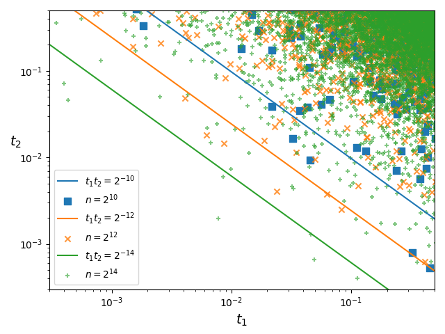
The event , as defined in the above proof, only occurs finitely many times almost surely. The origin is bounded away in this sense. Through symmetry arguments, we can similarly show that all the corners are bounded away from the following hyperbolic set:
| (15) |
where we use the boundary case instead of from Lemma 1. We also set to exclude trivial cases.
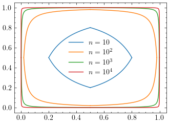
From Lemma 1, we see that the uniform distribution samples “diffuse” to the corner at a certain rate.
Figure 2 plots the samples from the uniform distribution and the corresponding reference boundaries . The samples approach the corner when size increases and a small portion of samples lie outside their corresponding reference boundaries.
2.2 Integrand with infinite variation
We are often interested in integrands with infinite variation, for which the Koksma–Hlawka inequality (6) is not informative. However, cases remain where the QMC methods work. The study [20] considered discontinuities inside the integration domain and proved that the convergence rate is still superior to the Monte Carlo method as long as some axes are parallel to the discontinuity interface. Another study [39] explored integrands that blow up at the boundary of and derived convergence rates based on a boundary growth condition. We are interested in the latter case. Following the work [39], the set was introduced to split the integration domain and the Sobol’ low-variation extension [48] extends from to . The extension depends on and through the hyperbolic set , but we suppress these dependences for the sake of simpler notations. Though the original name in the literatrue states “low-variation”, we assure the readers that the extension indeed has finite variation. For completeness, we provide the details here.
To this end, some notations need to be introduced. For an index set , denotes its complement . The notation is used to denote the point , where for and for , “concatenating” the vectors and . For simplicity, we assume the derivative of the integrand exists in , for . Given an anchor point and using the fundamental theorem of calculus, we obtain
| (16) |
The Sobol’ low-variation extension is given by
| (17) |
Following [39, 48], we apply a three-epsilon argument to bound the integration error. Recalling the notations on the exact integration (1) and QMC estimation (2), we bound:
| (18) | ||||
Observe that and coincide in . Moreover, we have
| (19) |
Using the above inequalities, we obtain the following finite upper bound for the RQMC method:
| (20) | ||||
Notice that the above bound (20) depends on the value of , which is used to construct the set in Equation (15). When , this becomes the classical Koksma–Hlawka inequality, and when , the hyperbolic set vanishes and the right hand side becomes . For , the asymptotic upper bound also reduces to the Koksma–Hlawka inequality, as .
To examine the behavior of the difference and the variation as the set grows when increases, we assume the following boundary growth condition (in the nonasymptotic case) outside the set .
Assumption 1 (Nonasymptotic boundary growth condition).
For the integrand , we assume the following boundary growth condition (21)
| (21) |
for a given constant , and . The inequality holds component-wise.
In Assumption 1, we emphasize the dependence , which is crucial in the following nonasymptotic analysis. For now, we consider an anisotropic integrand.
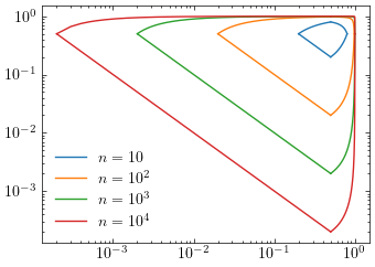
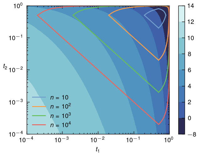
Example 1 (An anisotropic integrand).
| (22) |
As is often the case, the function 22 in our example is not isotropic w.r.t. the coordinates. Figure 3 provides an illustration of the sets with and the contour of the function 22 on the log scale. The value of may not be constant for .
This finding motivates the determination of an upper bound of the following term:
in dimension , which is equivalent to the following optimization problem:
| (23) | ||||
for a given . We define as the optimizer of (23) and
| (24) |
for . In one dimension, the point is explicitly given by . For , and is determined by solving the optimization problem (23).
Following the proof of Lemma 5.1 in [39], for an integrand satisfying the boundary growth condition (21), the difference of the integrand and its Sobol’ low-variation extension is bounded by
| (25) |
where . Notice that the power has a dependence on the specific choice of . Consider the optimization problem (23), we further consider the bound of with the only dependence on in Lemma 2.
Lemma 2 (A bound for the difference of the integrand and its Sobol’ low-variation extension).
From Lemma 2, following Lemma 5.4 and the proof of Theorem 5.5 in [39], we have
| (27) |
and
| (28) |
for finite and . Now, we have obtained the ingredients to present the nonasymptotic upper bound for the RQMC upper bound.
Theorem 3 (Nonasymptotic QMC error estimate).
For a continuous integrand on , whose mixed first-order derivative exists, the expected integration for the RQMC method with a quadrature size of satisfies
| (29) |
where , and and are finite constants that depend on and .
Proof.
Theorem 3 is the contribution of this work to the nonasymptotic QMC error estimate model. We observe that the convergence rate of the RQMC method depends on , which depends on the QMC quadrature size .
Remark 3 (Nonasymptotics rather than singularity).
In some cases, for instances, the two examples considered in the next Section 3, both integrands exhibit singularities at the boundary. However, the value of from (24) converges to 0 as . In this situation, the convergence rate for the RQMC method becomes the optimal asymptotic rate for , in the presence of the singularities and hence infinite variations. However, the optimal convergence rate may not be observed for a finite sample size , as may not converge to 0, resulting a suboptimal convergence rate indicated by Theorem 3. The next section illustrates the nonasymptotics with two concrete examples.
3 Two examples of infinite variation integrands
This section delves into two typical integration examples: the expectation estimate of lognormal random variables and the QoIs relating to the solution of elliptic PDEs with lognormal coefficients. These examples shed light on the intricate nature of infinite variation integrands.
3.1 Lognormal random variable
We first analyze the integration problem (1), where , , and applies the inverse standard normal distribution CDF component-wise. The partial derivative of w.r.t. is given by
| (31) |
Next, we consider the case where for . We use the following approximation:
| (32) | ||||
The case where can be derived similarly due to symmetry:
| (33) |
(see [45], Chapter 3.9, for instance).
Using the approximation of (33), we can simplify the partial derivative of as
| (34) |
We define to simplify the notation, and the term behaves like for any as . To check the boundary growth condition (21), it remains to study the local growth behavior of the term
| (35) |
Lemma 4 (First-order Taylor approximation).
The function satisfies the following bound:
| (36) |
where , .
Proof.
Notice that as for . Theorem 3 indicates that the QMC method achieves the asymptotic convergence rate .
Let us now consider the optimization problem (23):
| (41) | ||||
for a given . The Lagrangian is given by
| (42) | ||||
3.2 Elliptic partial differential equations with lognormal coefficients
We consider an elliptic PDE on a Lipschitz domain , in the following form:
| for , | (45a) | ||||
| (45b) | |||||
with almost all , where belongs to a complete probability space tuple . The differential operators and are taken w.r.t. the spatial variable , and is the outward normal derivative operator. We explore the equations in (45) in the weak form. For a suitable functional space (e.g., ), we seek such that
| (46) |
where denotes the inner product. The QoI is given in the following general form:
| (47) |
where , denotes the dual space of . We are interested in computing . The integrand in (1) is given by .
We consider , which takes the following form:
| (48) |
with and are i.i.d. samples from , . Moreover, we define , for .
From [17], an upper bound for the derivative of w.r.t. the random variable is given by
| (49) |
The derivative of the integrand is as follows:
| (50) | ||||
where we apply the approximation of (32) as approaches 0, where . Unlike the example in Section 3.1, the considered integrand has singularities when and . Due to the symmetry in each dimension, we only need to consider the singularity at 0. To investigate the local growth behavior of the derivative, we define
| (51) |
Similar to the analysis in Section. 3.1, we apply a first-order Taylor approximation. We take the logarithm of both sides of (51):
| (52) |
Thus, for
| (53) |
we have
| (54) |
where
Similarly, we can determine as follows:
| (55) |
and .
In this section, we have considered two concrete examples with unbounded variation and applied the theory developed in Section 2 to analyze their convergence rates. Consistent with the theory, the convergence rate can be improved by increasing the sample size . However, whether we can further enhance the convergence rate by modifying the sample distribution and placing more points near the singular corners is unclear. In the next section, we discuss the effects of importance sampling.
4 Importance sampling
This section provides two kinds of IS proposal distributions and analyzes their effects on the convergence rate.
4.1 First proposal distribution
This section proposes a Gaussian distribution with scaled variance to distribute more samples closer to the corners. This kind of IS was studied in [28] for multivariate functions that belong to certain Sobolev spaces, where the worst-case integration error was analyzed and optimized.
Let , which are the two integrands considered in Section 3. We introduce the component-wise multiplication notation , such that when . The integral of over is
| (56) | ||||
where , , and is the -dimensional standard normal distribution density. The integrand with IS is given by
| (57) | ||||
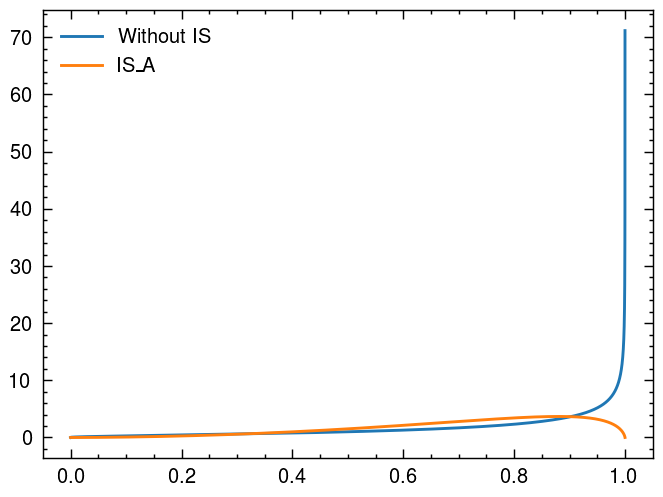
where we define and . The function no longer has the singularity at the boundaries for , . Figure 4 illustrates the one-dimensional integrand with and without IS in Example 1.
Let us define for the simplicity of notations. We will analyze the mixed first-order derivative . Specifically, we have
| (58) | ||||
We have
| (59) |
and
| (60) | ||||
Notice that , for all . In Example 1 (i.e., when ), we have
| (61) |
By combining equations (58) to (61), we have
| (62) | ||||
where we have substituted by to focus on the boundary growth condition at the singularity. Before further analysis, we now analyze the derivative in Example 2.
In Example 2, , we apply the following upper bound of :
| (63) |
Combining equations (58) to (60) and (63), we obtain
| (64) | ||||
where we use the approximation and omit the term , as . We observe that the upper bound (64) shares similar structures with (62). We will analyze the upper bound (64) in detail and show later that the conclusions will apply to (62) of Example 1 as well.
Similar to the analysis in Section 3.1, we have
| (65) |
where . Notice that as . Thus,
| (66) |
The term being greater than or equal to ensures the term in the convergence model (29), which happens when
| (67) |
which is guaranteed by and a finite such that . For the optimality condition in Example 1 we can simply replace in (67) with . Finite for imply finite (via the hyperbolic set (15)), thus the rate is achievable with a finite , in contrast to the asymptotic optimal rates in (44) and (55).
Nevertheless, modifying changes the variance of the integrand . Thus, we aim to determine the optimal by minimizing the variance of :
| (68) |
which is equivalent to finding the minimizer for the second-order moment of , as :
| (69) | ||||
When the analytic solution is unavailable, we aim to find an approximate optimizer using samples. Specifically, we minimize the following objective function
| (70) |
In practice, the number in the pilot run does not exceed the number of simulations samples.
4.2 Second proposal distribution
This section considers another IS proposal distribution. We will only analyze Example 2 for brevity, as the case for Example 1 can be derived similarly. Inspired by the beta distribution, we propose the following distribution :
| (71) |
with the constant . The reason to propose such a distribution is the ease of computing the CDF and its inverse :
| (72) |
| (73) |
Next, we apply IS to compute the integral . Using the density , we can write
| (74) | ||||
In Example 2, , and we introduce
| (75) |
Similar to the last section, a possible choice of the parameter can be determined by minimizing the second-order moment of :
| (76) | ||||
Again, we seek an optimizer based on ensembles when the analytical solution is unavailable.
Next, we study the mixed first-order derivative of :
| (77) | ||||
where . We have
| (78) |
and
| (79) | ||||
where we define and . We only consider the case where for simplicity, as other cases can be induced by symmetry. We have
| (80) |
and
| (81) | ||||
Combining (63) and (78) to (81), we obtain
| (82) | ||||
We apply the change of variable for and continue the analysis as follows:
| (83) | ||||
where in the last inequality we use,
with . Compared to the case without IS (), an improved regularity of is achieved for , as the exponent becomes larger, i.e., , when . Moreover, the condition for ensures the convergence rate, which requires
| (84) |
Similar to the optimality condition (67) in the first proposal distribution, and sufficiently large and finite for all and thus sufficiently large and finite are required for the convergence rate.
5 Numerical results
This section tests the convergence rates of the two examples we have considered, compares them with the analysis, and demonstrates how IS improves the rates.
5.1 Lognormal random variable expectation
We approximate the expectation of a lognormal random variable, that is,
where are i.i.d. . The expectation is analytically given by
We test the convergence of the root mean squared error (RMSE) of the RQMC method using the Sobol’ sequence. The RMSE for QMC is computed as follows:
| (85) |
where and .
With the nested uniform scrambling (Owen’s scrambling) employed as the randomization, the convergence rate for the RMSE is if the integrand has Lipschitz-continuous mixed first-order derivatives [38]. However, the integrand has a singularity at 0 and thus does not have this property. In both examples presented in this work, we opt for the random linear scramble [33, 23] as the randomization. This randomization incurs lower computational cost compared to Owen’s scrambling while still yielding the same variance for the RQMC estimator. (For instance, refer to Definition 6 of [40] or Section 6.12 of [10]).
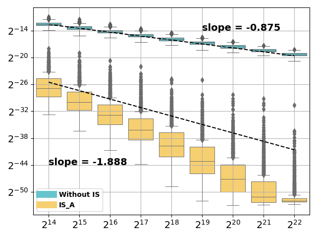
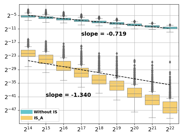
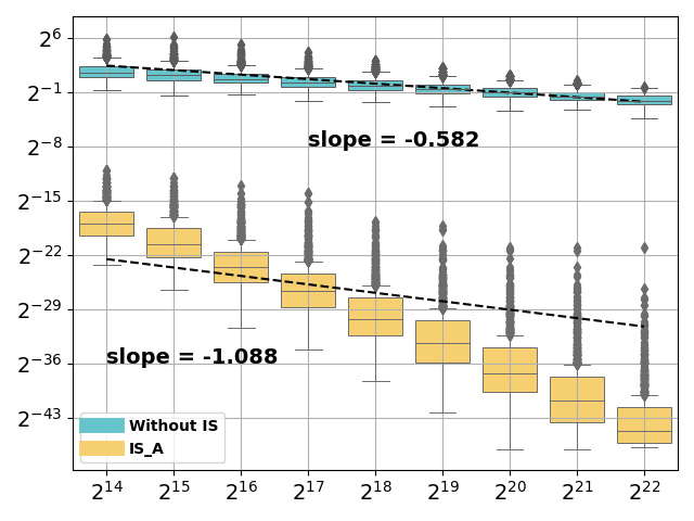
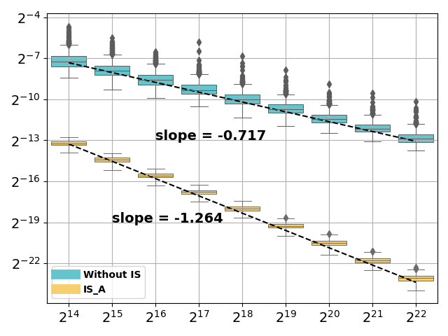
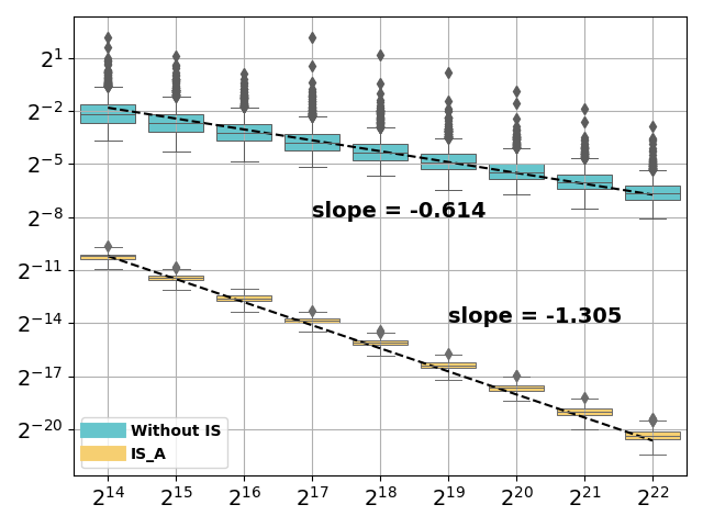
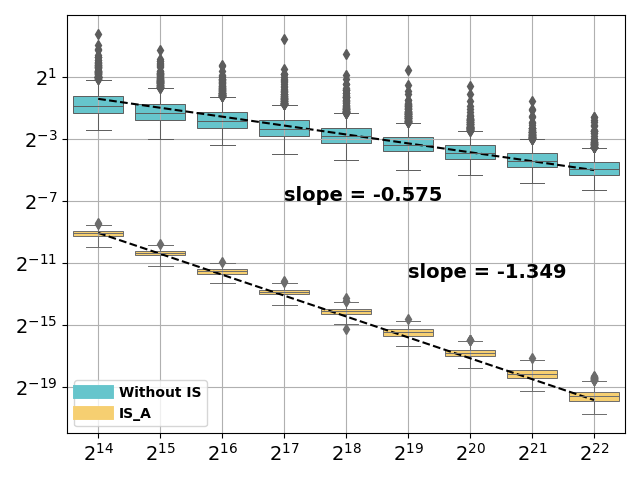
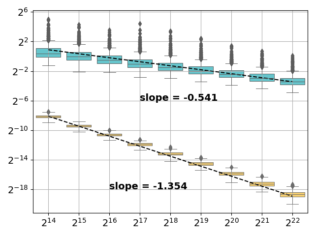
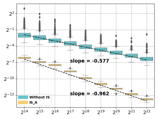
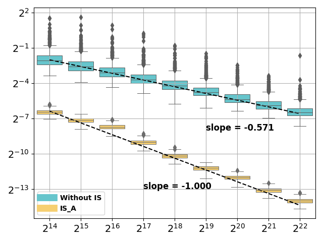
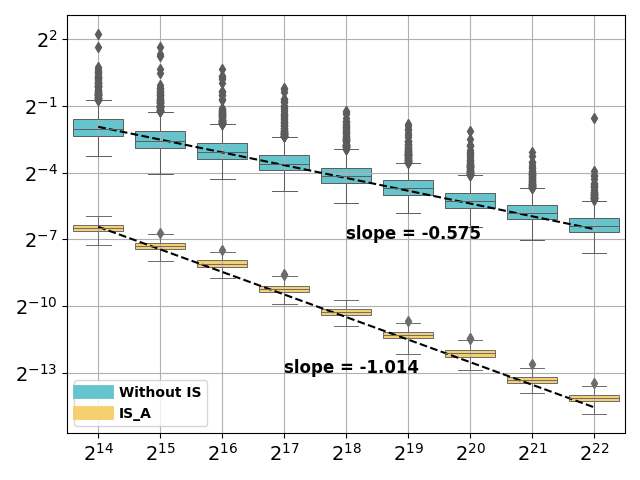
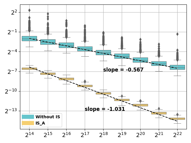
Figures 5, 6, and 7 plot the convergence of the RMSE for the original integrand and the integrand with importance sampling, . Each data point in these figures is RQMC estimator with the number of randomizations . Each boxplot consists of 10,000 samples. As can be observed, the IS significantly reduces the RMSE and improves the convergence rate.
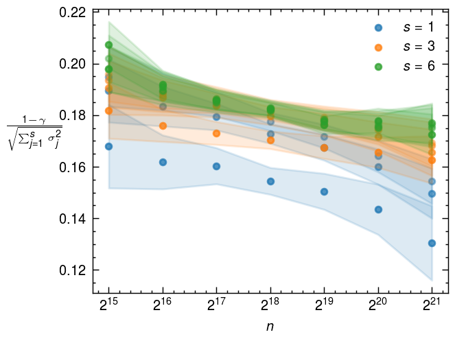
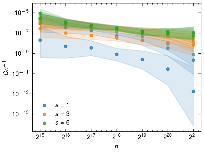
Tables 1, 2, and 3 provide the measured convergence rates and the value . For the same sample size , the convergence rate decreases as increases. The value exhibits similarity in magnitude for all cases in each dimension setting and increases as the dimension increases. Figure 8 plots the values (left) and with the corresponding 95% confidence intervals. The variation within each group is also observed to be smaller than the values across groups.
| Conv. Rate | Conv. Rate with IS | ||
|---|---|---|---|
| 1.0 | 0.875 | 1.888 | 0.125 |
| 2.0 | 0.719 | 1.340 | 0.141 |
| 3.0 | 0.582 | 1.088 | 0.139 |
| Conv. Rate | Conv. Rate with IS | ||
|---|---|---|---|
| (1.0, 1.0, 1.0) | 0.717 | 1.264 | 0.163 |
| (2.0, 1.0, 1.0) | 0.614 | 1.305 | 0.158 |
| (2.0, 1.4, 1.0) | 0.575 | 1.349 | 0.161 |
| (2.0, 1.7, 1.0) | 0.541 | 1.354 | 0.162 |
| cases | Conv. Rate | Conv. Rate with IS | |
|---|---|---|---|
| I | 0.577 | 0.962 | 0.173 |
| II | 0.571 | 1.000 | 0.175 |
| III | 0.575 | 1.014 | 0.174 |
| IV | 0.567 | 1.031 | 0.178 |
5.2 Elliptic partial differential equations with lognormal coefficient
We first specify the settings of this example. The QoI is the weighted integration of the solution over the entire domain , that is,
where , , denotes the convolution operator, is the indicator function, , and represents the Gaussian density function in with mean and covariance . The PDE problem (45a) is solved with DEAL.II [1], using the finite element on a 1616 mesh.
Recall that the coefficient involved in the PDE model (45) is given by,
where the basis are the eigenfunctions to the following Matérn covariance kernel:
| (86) |
where we chose and . In addition, is the Gamma function, and is the modified Bessel function of the second kind. Let and be the Fourier coefficients and trigonometric functions in the Fourier expansion of the covariance kernel on an extended domain , respectively, with . The extension is needed to ensure the positivity of the Fourier coefficients [3]. We let
| (87) | ||||
Apart from the trigonometric-basis expansions, we also apply Meyer wavelet functions to construct the basis (for a detailed analysis and instructions, see Section 4 in [3]).
To validate the proposed convergence model (55), we also considered the following coefficient:
| (88) |
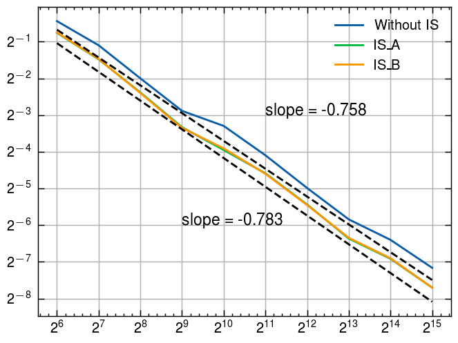
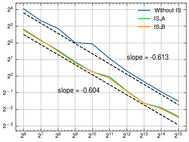
where we generated six samples of within each dimension setting. In the first sample, . In the second and third samples, are i.i.d. sampled from the uniform distribution . In the last three samples, the values of the first three cases are multiplied component-wise by 2. Figure 9 plots the deteriorated rate against . The convergence rate is measured between and number of samples, with one RQMC estimator of randomizations. In all considered cases, the rate exhibits an almost linear dependence on . Unlike Example 1, the effect of dimensions on the convergence rates is not obvious in both cases, which was unexpected because the QMC points quality deteriorates in higher dimensions. One possible reason for this observation lies in Equation (49), where we applied the upper bounds for and its derivatives, which conceals the effective dimension.
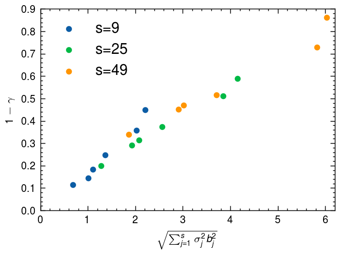
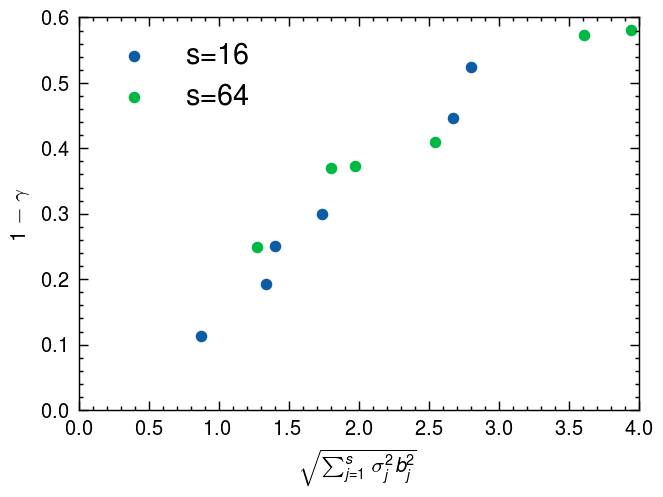
Figure 10 compares the norm of the basis and between trigonometric and wavelet-type bases. The trigonometric basis is optimal in approximating the random field in the sense. However, the basis norm, which appears in the convergence model (55) and (29) is the primary interest. Ideally, is desired to converge fast as increases to reduce the effective dimension. In the nonasymptotic QMC convergence model for elliptic PDEs (55), the value is expected to be small for a fixed dimension . We observed that the values of the wavelet-type basis in the plotted range are smaller than those of the trigonometric basis. The localization properties of the wavelet-type basis make it even more favorable when the function is restricted on since .
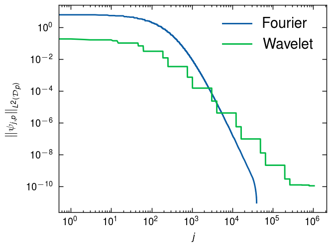
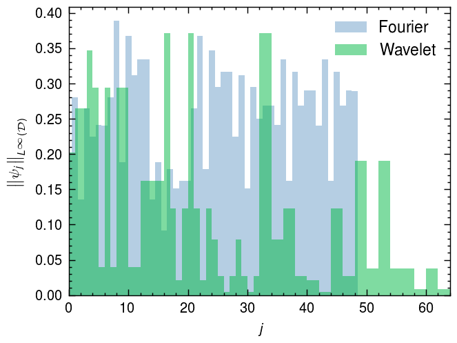
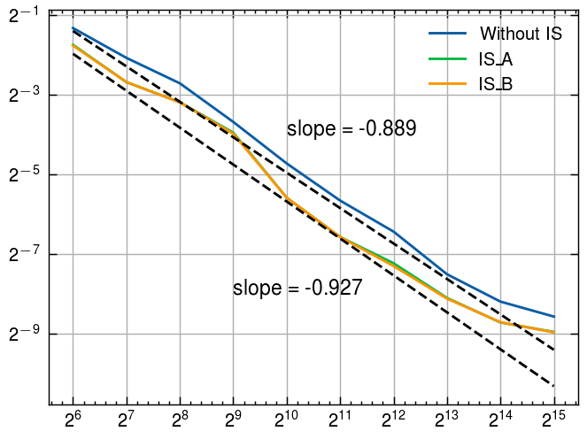
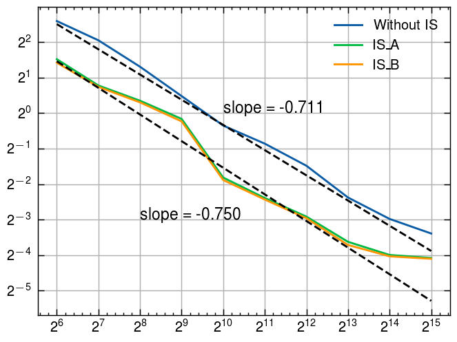
Figure 11 plots the convergence of the RMSE for the original integrand and the integrand with IS , where the wavelet-type basis is used for two variance settings and two dimension settings. In all cases, both types of IS improve the integrand regularity, reducing the RMSE and improving the convergence rate. Furthermore, the effectiveness of the IS is more significant when the dimension is smaller, as IS has more limitations in higher dimensions to not increase the variance. Moreover, when the original integrand has a larger the IS works better because in (66) becomes larger and in (83) becomes smaller.
6 Conclusion
In this work, we study the nonasymptotic QMC convergence rate model for functions with finite-dimensional inputs. Specifically, we focus on the expectation of a lognormal random variable and an elliptic PDE problem characterized by lognormal coefficients. Drawing upon the hyperbolic set introduced in the work of Owen [39], we subdivided the integration domain. This division allowed us to split the QMC integration error into two distinct contributions, namely: and . This method replaces the right-hand side of the Koksma–Hlawka inequality , which is infinite for the unbounded functions considered in this work, with two finite terms.
Our primary contribution through this work has been deriving an upper bound for the integrand derivative via an optimization problem, denoted as (23). With this in place, we applied it within the convergence model, culminating in deriving the nonasymptotic QMC convergence rate model. In our quest to verify the proposed model, we presented numerical examples for the two problems above. Moreover, the analytical procedures delineated here can find relevance in varied integration challenges, one notable instance being the option pricing problem within financial scenarios.
In addition to the above, our work also involved applying two IS distributions, leading us to evaluate their potential to enhance integrand regularity. Notably, despite the distinct support of these distributions, their influence on the integrand appeared broadly analogous.
However, there remain areas that we have not explored in depth. For instance, we have yet to derive the constant within the hyperbolic set. Delving into its dependence on dimensionality and integrand characteristics could be a promising trajectory for subsequent studies. Moreover, future inquiries could also encompass the random field’s truncation error, where wavelets demonstrate a superior edge over the trigonometric basis, as indicated in [2]. Furthermore, examining a multilevel setting with adaptivity, as hinted at in [8], could be beneficial.
Lastly, it is worth noting our choice to employ the Sobol’ sequence instead of exploring weighted spaces or designing lattice rules (e.g., [30], [17]). The latter could reduce the worst-case integration error for specific function spaces, potentially leading to a dimension-independent outcome given certain conditions. This combination of lattice rules and nonasymptotic analysis remains a compelling avenue for future exploration.
7 Acknowledgement
This publication is based on work supported by the Alexander von Humboldt Foundation and the King Abdullah University of Science and Technology (KAUST) office of sponsored research (OSR) under Award No. OSR-2019-CRG8-4033. This work utilized the resources of the Supercomputing Laboratory at King Abdullah University of Science and Technology (KAUST) in Thuwal, Saudi Arabia. The authors thank Christian Bayer, Fabio Nobile and Erik von Schwerin for fruitful discussions. We are also grateful to Arved Bartuska and Michael Samet for proofreading this manuscript. Their suggestions significantly improve the paper’s readibility. We acknowledge the use of the following open-source software packages: deal.II [1].
References
- [1] D. Arndt, W. Bangerth, B. Blais, T. C. Clevenger, M. Fehling, A. V. Grayver, T. Heister, L. Heltai, M. Kronbichler, M. Maier, P. Munch, J.-P. Pelteret, R. Rastak, I. Thomas, B. Turcksin, Z. Wang, and D. Wells, The deal.II library, version 9.2, Journal of Numerical Mathematics, 28 (2020), pp. 131–146.
- [2] M. Bachmayr, A. Cohen, R. DeVore, and G. Migliorati, Sparse polynomial approximation of parametric elliptic PDEs. Part II: lognormal coefficients, ESAIM: Mathematical Modelling and Numerical Analysis, 51 (2017), pp. 341–363.
- [3] M. Bachmayr, A. Cohen, and G. Migliorati, Representations of Gaussian random fields and approximation of elliptic PDEs with lognormal coefficients, Journal of Fourier Analysis and Applications, 24 (2018), pp. 621–649.
- [4] C. Bayer, C. Ben Hammouda, and R. Tempone, Numerical smoothing with hierarchical adaptive sparse grids and quasi-Monte Carlo methods for efficient option pricing, Quantitative Finance, 23 (2023), pp. 209–227.
- [5] C. Bayer, C. B. Hammouda, A. Papapantoleon, M. Samet, and R. Tempone, Optimal damping with hierarchical adaptive quadrature for efficient Fourier pricing of multi-asset options in Lévy models, ArXiv, abs/2203.08196 (2022).
- [6] C. Bayer, C. B. Hammouda, and R. Tempone, Numerical smoothing and hierarchical approximations for efficient option pricing and density estimation, arXiv: Computational Finance, (2020).
- [7] C. Bayer, M. Siebenmorgen, and R. Tempone, Smoothing the payoff for efficient computation of basket option prices, Quantitative Finance, 18 (2016), pp. 491–505.
- [8] J. Beck, Y. Liu, E. von Schwerin, and R. Tempone, Goal-oriented adaptive finite element multilevel Monte Carlo with convergence rates, Computer Methods in Applied Mechanics and Engineering, 402 (2022), p. 115582.
- [9] R. E. Caflisch, W. J. Morokoff, and A. B. Owen, Valuation of mortgage backed securities using Brownian bridges to reduce effective dimension, vol. 24, Department of Mathematics, University of California, Los Angeles, 1997.
- [10] J. Dick, F. Y. Kuo, and I. H. Sloan, High-dimensional integration: the quasi-monte carlo way, Acta Numerica, 22 (2013), pp. 133–288.
- [11] J. Dick and F. Pillichshammer, Digital nets and sequences: discrepancy theory and quasi-Monte Carlo integration, Cambridge University Press, 2010.
- [12] G. Y. Dong and C. Lemieux, Dependence properties of scrambled Halton sequences, Mathematics and Computers in Simulation, 200 (2022), pp. 240–262.
- [13] M. Gerber and N. Chopin, Sequential quasi Monte Carlo, Journal of the Royal Statistical Society: Series B (Statistical Methodology), 77 (2015), pp. 509–579.
- [14] A. D. Gilbert, F. Y. Kuo, and I. H. Sloan, Preintegration is not smoothing when monotonicity fails, in Advances in Modeling and Simulation: Festschrift for Pierre L’Ecuyer, Springer, 2022, pp. 169–191.
- [15] E. Gobet, M. Lerasle, and D. Métivier, Mean estimation for randomized quasi Monte Carlo method, (2022).
- [16] T. Goda and P. L’ecuyer, Construction-free median quasi-Monte Carlo rules for function spaces with unspecified smoothness and general weights, SIAM Journal on Scientific Computing, 44 (2022), pp. A2765–A2788.
- [17] I. G. Graham, F. Y. Kuo, J. A. Nichols, R. Scheichl, C. Schwab, and I. H. Sloan, Quasi-Monte Carlo finite element methods for elliptic PDEs with lognormal random coefficients, Numerische Mathematik, 131 (2015), pp. 329–368.
- [18] M. Griebel, F. Kuo, and I. Sloan, The smoothing effect of integration in and the ANOVA decomposition, Mathematics of Computation, 82 (2013), pp. 383–400.
- [19] A. Griewank, F. Y. Kuo, H. Leövey, and I. H. Sloan, High dimensional integration of kinks and jumps—smoothing by preintegration, Journal of Computational and Applied Mathematics, 344 (2018), pp. 259–274.
- [20] Z. He and X. Wang, On the convergence rate of randomized quasi-Monte Carlo for discontinuous functions, SIAM Journal on Numerical Analysis, 53 (2015), pp. 2488–2503.
- [21] Z. He, Z. Zheng, and X. Wang, On the error rate of importance sampling with randomized quasi-Monte Carlo, arXiv preprint arXiv:2203.03220, (2022).
- [22] L. Herrmann and C. Schwab, QMC integration for lognormal-parametric, elliptic PDEs: local supports and product weights, Numerische Mathematik, 141 (2019), pp. 63–102.
- [23] H. S. Hong and F. J. Hickernell, Algorithm 823: Implementing scrambled digital sequences, ACM Transactions on Mathematical Software (TOMS), 29 (2003), pp. 95–109.
- [24] J. Imai and K. S. Tan, A general dimension reduction technique for derivative pricing, Journal of Computational Finance, 10 (2006), p. 129.
- [25] , Pricing derivative securities using integrated quasi-Monte Carlo methods with dimension reduction and discontinuity realignment, SIAM Journal on Scientific Computing, 36 (2014), pp. A2101–A2121.
- [26] X. Jin and A. X. Zhang, Reclaiming Quasi-Monte Carlo efficiency in portfolio value-at-risk simulation through Fourier transform, Management Science, 52 (2006), pp. 925–938.
- [27] Y. Kazashi, Quasi-Monte Carlo integration with product weights for elliptic pdes with log-normal coefficients, IMA Journal of Numerical Analysis, 39 (2019), pp. 1563–1593.
- [28] P. Kritzer, F. Pillichshammer, L. Plaskota, and G. W. Wasilkowski, On efficient weighted integration via a change of variables, Numerische Mathematik, 146 (2018), pp. 545–570.
- [29] F. Y. Kuo and D. Nuyens, A practical guide to quasi-Monte Carlo methods, (2016).
- [30] F. Y. Kuo, C. Schwab, and I. H. Sloan, Quasi-Monte Carlo finite element methods for a class of elliptic partial differential equations with random coefficients, SIAM J. Numer. Anal., 50 (2012), pp. 3351–3374.
- [31] S. Liu and A. B. Owen, Preintegration via active subspace, SIAM Journal on Numerical Analysis, 61 (2023), pp. 495–514.
- [32] P. L’Ecuyer, Randomized quasi-Monte Carlo: An introduction for practitioners, Springer, 2018.
- [33] J. Matoušek, On the L2-discrepancy for anchored boxes, Journal of Complexity, 14 (1998), pp. 527–556.
- [34] W. J. Morokoff and R. E. Caflisch, Quasi-random sequences and their discrepancies, SIAM Journal on Scientific Computing, 15 (1994), pp. 1251–1279.
- [35] J. A. Nichols and F. Y. Kuo, Fast CBC construction of randomly shifted lattice rules achieving convergence for unbounded integrands over in weighted spaces with POD weights, Journal of Complexity, 30 (2014), pp. 444–468.
- [36] H. Niederreiter, Random number generation and quasi-Monte Carlo methods, SIAM, 1992.
- [37] D. Ouyang, X. Wang, and Z. He, Quasi-Monte Carlo for unbounded integrands with importance sampling, arXiv preprint arXiv:2310.00650, (2023).
- [38] A. B. Owen, Scrambling Sobol’ and Niederreiter–Xing points, Journal of complexity, 14 (1998), pp. 466–489.
- [39] A. B. Owen, Halton sequences avoid the origin, SIAM Review, 48 (2006), pp. 487–503.
- [40] A. B. Owen, Local antithetic sampling with scrambled nets, The Annals of Statistics, (2008), pp. 2319–2343.
- [41] A. B. Owen, Monte Carlo theory, methods and examples, 2013.
- [42] A. B. Owen, A randomized Halton algorithm in R, arXiv preprint arXiv:1706.02808, (2017).
- [43] Z. Pan and A. Owen, Super-polynomial accuracy of one dimensional randomized nets using the median of means, Mathematics of Computation, 92 (2023), pp. 805–837.
- [44] A. Papageorgiou, The Brownian bridge does not offer a consistent advantage in quasi-Monte Carlo integration, Journal of Complexity, 18 (2002), pp. 171–186.
- [45] J. K. Patel and C. B. Read, Handbook of the normal distribution, vol. 150, CRC Press, 1996.
- [46] I. Pinelis, Exact lower and upper bounds on the incomplete gamma function, arXiv preprint arXiv:2005.06384, (2020).
- [47] I. H. Sloan and H. Woźniakowski, When are quasi-Monte Carlo algorithms efficient for high dimensional integrals?, Journal of Complexity, 14 (1998), pp. 1–33.
- [48] I. Sobol, Calculation of improper integrals using equidistributed sequences, Doklady Akademii Nauk SSSR, 210 (1973), pp. 278–281.
- [49] X. Wang, Dimension reduction techniques in quasi-Monte Carlo methods for option pricing, INFORMS Journal on Computing, 21 (2009), pp. 488–504.
- [50] X. Wang and K.-T. Fang, The effective dimension and quasi-Monte Carlo integration, Journal of Complexity, 19 (2003), pp. 101–124.
- [51] X. Wang and I. H. Sloan, Why are high-dimensional finance problems often of low effective dimension?, SIAM Journal on Scientific Computing, 27 (2005), pp. 159–183.
- [52] , Low discrepancy sequences in high dimensions: How well are their projections distributed?, Journal of Computational and Applied Mathematics, 213 (2008), pp. 366–386.
- [53] , Quasi-Monte Carlo methods in financial engineering: An equivalence principle and dimension reduction, Operations Research, 59 (2011), pp. 80–95.
- [54] X. Wang and K. S. Tan, Pricing and hedging with discontinuous functions: Quasi-Monte Carlo methods and dimension reduction, Management Science, 59 (2013), pp. 376–389.
- [55] C. Weng, X. Wang, and Z. He, Efficient computation of option prices and Greeks by quasi-Monte Carlo method with smoothing and dimension reduction, SIAM Journal on Scientific Computing, 39 (2017), pp. B298–B322.
- [56] J. Wiart, C. Lemieux, and G. Y. Dong, On the dependence structure and quality of scrambled -nets, Monte Carlo Methods and Applications, 27 (2019), pp. 1 – 26.