What’s in a Prior?
Learned Proximal Networks for Inverse Problems

Abstract

Proximal operators are ubiquitous in inverse problems, commonly appearing as part of algorithmic strategies to regularize problems that are otherwise ill-posed. Modern deep learning models have been brought to bear for these tasks too, as in the framework of plug-and-play or deep unrolling, where they loosely resemble proximal operators. Yet, something essential is lost in employing these purely data-driven approaches: there is no guarantee that a general deep network represents the proximal operator of any function, nor is there any characterization of the function for which the network might provide some approximate proximal. This not only makes guaranteeing convergence of iterative schemes challenging but, more fundamentally, complicates the analysis of what has been learned by these networks about their training data. Herein we provide a framework to develop learned proximal networks (LPN), prove that they provide exact proximal operators for a data-driven nonconvex regularizer, and show how a new training strategy, dubbed proximal matching, provably promotes the recovery of the log-prior of the true data distribution. Such LPN provide general, unsupervised, expressive proximal operators that can be used for general inverse problems with convergence guarantees. We illustrate our results in a series of cases of increasing complexity, demonstrating that these models not only result in state-of-the-art performance, but provide a window into the resulting priors learned from data.

1 Introduction

Inverse problems concern the task of estimating some underlying variables that have undergone a degradation process, such as in denoising, deblurring, inpainting, or compressed sensing bertero2021introduction,ongie2020deep. While these problems are naturally ill-posed, solutions to any of these problems involve, either implicitly or explicitly, the utilization of priors, or models, about what type of solutions are preferable engl1996regularization,benning2018modern,arridge2019solving. Traditional methods model this prior distribution directly, by constructing functions (or regularization terms) that promote specific properties in the resulting estimate, such as for it to be smooth tikhonov1977solutions, piece-wise smooth rudin1992nonlinear,bredies2010total, or for it to have a sparse decomposition under a given basis or even a potentially overcomplete dictionary bruckstein2009sparse, sulam2014image. On the other hand, from a machine learning perspective, the complete restoration mapping has also been modeled by a regression function, typically by providing a large collection of input-output (or clean-corrupted) pairs of samples mccann2017convolutional,ongie2020deep,zhu2018image.

An interesting third alternative combines these two approaches by making the insightful observation that for almost any inverse problem, a proximal step for the regularization function is always present. Such a sub-problem can be loosely interpreted as a denoising step and, as a result, off-the-shelf and very strong-performing denoising algorithms (as those given by modern deep learning methods) can be employed as a subroutine. The Plug-and-Play (PnP) framework is one such example of this idea venkatakrishnan2013plug,zhang2017learning,zhang2021plug,kamilov2023plug,tachella2019real, but others exist as well romano2017little,romano2015boosting. While these alternatives work very well in practice, little is known about the approximation properties of these methods: Do these denoising networks actually (i.e., provably) provide a proximal operator for some regularization function? From a variational perspective, would this regularization function recover the correct regularizer, such as the (log) prior of the data distribution?

In this work, we study and positively answer the two questions above in the context of unsupervised restoration models for general inverse problems (i.e., without having access to the specific forward operator during training). We do this by providing a class of neural network architectures that implement exact proximal operators for some learned function. As a result, and when trained in the context of a denoising task, such learned proximal networks implicitly, but exactly, learn a regularization function that provides good estimation of the underlying solution in a data-driven manner. In turn, we introduce a new training problem, which we dub proximal matching, that provably promotes the recovery of the correct regularization term (i.e. the log of the data distribution), which need not be convex. The ability to implement exact proximal operators also opens the door to convergence to critical points of the variational problem, which we derive for a representative PnP reconstruction algorithm. In this way, we provide a general tool to develop unsupervised restoration approaches, and demonstrate that they achieve state-of-the-art performance for tasks such as image deblurring, CT reconstruction and compressed sensing. Furthermore, and importantly, our methodology enables the precise characterization of the data-dependent prior learned by these models.

2 Background

Consider an unknown signal in an Euclidean space, $\mathbf{x}\in\mathbb{R}^{n}$, and a known measurement operator that maps to an output space, $A:\mathbb{R}^{n}\rightarrow\mathbb{R}^{m}$. The goal of inverse problems is to recover $\mathbf{x}$ from its noisy observation $\mathbf{y}=A(\mathbf{x})+\mathbf{v}\in\mathbb{R}^{m}$, where $\mathbf{v}$ is a noise or nuisance term. This problem is typically ill-posed: infinitely many solutions $\mathbf{x}$ may explain (i.e. approximate) the measurement $\mathbf{y}$ benning2018modern. Hence, a prior is needed to regularize the problem, which can generally take the form

$$\min_{\mathbf{x}}\frac{1}{2}\|\mathbf{y}-A(\mathbf{x})\|_{2}^{2}+\phi(\mathbf{x}),$$ (2.1)

for a function $\phi(\mathbf{x}):\mathbb{R}^{n}\to\mathbb{R}$ promoting a solution that is likely under the prior distribution of $\mathbf{x}$. We will make no assumptions on the convexity of $\phi(\mathbf{x})$ in this work.

Proximal operators

Originally proposed by Moreau [68] as a generalization of projection operators, proximal operators are central in optimizing the problem (2.1) by means of proximal gradient descent (PGD) beck2017first, alternating direction method of multipliers (ADMM) boyd2011distributed, or primal dual hybrid gradient (PDHG) chambolle2011first. For a given functional $\phi$ as above, its proximal operator $\operatorname{prox}_{\phi}$ is defined by

$$\operatorname{prox}_{\phi}(\mathbf{y}):=\operatorname*{argmin}_{\mathbf{x}}\frac{1}{2}\|\mathbf{y}-\mathbf{x}\|^{2}+\phi(\mathbf{x}).$$ (2.2)

When $\phi$ is non-convex, the solution to this problem may not be unique and the proximal mapping is set-valued. Following gribonval2020characterization, we define the proximal operator of a function $\phi$ as a selection of the set-valued mapping: $f(\mathbf{y})$ is a proximal operator of $\phi$ if and only if $f(\mathbf{y})\in\operatorname*{argmin}_{\mathbf{x}}\frac{1}{2}\|\mathbf{y}-\mathbf{x}\|^{2}+\phi(\mathbf{x})$ for each $\mathbf{y}\in\mathbb{R}^{n}$. Interestingly, the same authors showed that the continuous proximal of a (potentially nonconvex) function can be fully characterized as the gradient of a convex function, as the following result formalizes.

Proposition 1 (Characterization of continuous proximal operators, [Corollary 1]gribonval2020characterization).

Let $\mathcal{Y}\subset\mathbb{R}^{n}$ be non-empty and open and $f:\mathcal{Y}\rightarrow\mathbb{R}^{n}$ be a continuous function. Then, $f$ is a proximal operator of a function $\phi:\mathbb{R}^{n}\rightarrow\mathbb{R}\cup\{+\infty\}$ if and only if there exists a convex differentiable function $\psi$ such that $f(\mathbf{y})=\nabla\psi(\mathbf{y})$ for each $\mathbf{y}\in\mathcal{Y}$.

It is worth stressing the difference between $\phi$ and $\psi$. While $f$ is the proximal operator of $\phi$, i.e. $\operatorname{prox}_{\phi}=f$, $f$ is also the gradient of a convex $\psi$, $\nabla\psi=f$ (see Figure 1). Furthermore, $\phi$ may be non-convex, while $\psi$ must be convex. As can be expected, there exists a precise relation between $\phi$ and $\psi$, and we will elaborate further on this connection shortly.

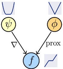
Figure 1: Illustration of Prop. 1 with $\phi(\cdot)=\|\cdot\|_{1}$.

The characterization of proximal operators of convex functions is similar, but with the additional condition that $f$ must be non-expansive moreau1965proximite. Hence, by relaxing the nonexpansivity, we obtain a broader class of proximal operators. As we will show later, the ability to model proximal operators of non-convex functions will prove extremely useful in practice, as the log-priors of most real-world data are indeed non-convex.

Plug-and-Play The methodology developed in this paper will be most closely related to the Plug-and-Play (PnP) framework. PnP employs off-the-shelf denoising algorithms to solve general inverse problems within an ADMM approach boyd2011distributed. Indeed, an ADMM solver for problem (2.1) involves a proximal step, i.e. a sub-problem as that in (2.2). Inspired by the observation that $\operatorname{prox}_{\phi}(\mathbf{y})$ resembles the maximum a posteriori (MAP) denoiser at $\mathbf{y}$ with a log-prior $\phi$, PnP replaces the explicit solution of this step with generic denoising algorithms, such as BM3D dabov2007image,venkatakrishnan2013plug or CNN-based denoisers zhang2017learning,zhang2021plug,kamilov2023plug, bringing the benefits of advanced denoisers to general inverse problems. While useful in practice, such denoisers are not in general proximal operators. Indeed, modern denoisers need not be the MAP estimators at all, but instead they typically approximate a minimum mean squared error (MMSE) solution. Although deep learning based denoisers have achieved impressive results when used with PnP, little is known about the implicit prior–if any–encoded in these denoisers, thus diminishing the interpretability of the reconstruction results. Certain convergence guarantees have been derived for PnP with MMSE denoisers Xu2020-my, chiefly relying on the assumption that the denoiser is non-expansive (which can be hard to verify or enforce in practice). Furthermore, as shown in Gribonval [42], when interpreted as proximal operators, the prior in MMSE denoisers can be drastically different from the original (true data) prior, raising concerns about the correctness of the reconstruction result. Lastly, there is a broader family of works that are also related–and have inspired to some extent–the ideas in this work. We expand on them in Appendix A.

3 Learned Proximal Networks

First, we seek a way to parameterize a neural network such that its mapping is the proximal operator of some (potentially nonconvex) scalar-valued functional. Motivated by Proposition 1, we will seek network architectures that parameterize gradients of convex functions. A simple way to achieve this is by differentiating a neural network that implements a convex function: given a scalar-valued neural network, $\psi_{\theta}:\mathbb{R}^{n}\rightarrow\mathbb{R}$, whose output is convex with respect to its input, we can parameterize a LPN as $f_{\theta}=\nabla\psi_{\theta}$, which can be efficiently computed via back propagation. This makes LPN a gradient field –and also a conservative vector field– of an explicit convex function. Fortunately, this is not an entirely new problem. Amos et al. [4] proposed input convex neural networks (ICNN) that enforce convexity by constraining the network weights to be non-negative and the nonlinear activations convex and non-decreasing. Consider a single-layer neural network characterized by the weights $\textbf{W}\in\mathbb{R}^{m\times n}$, bias term $\mathbf{b}\in\mathbb{R}^{m}$ and a scalar non-linearity $g:\mathbb{R}\to\mathbb{R}$. Such a network, at a sample $\mathbf{y}$, is given by $\mathbf{z}=g(\mathbf{W}\mathbf{y}+\mathbf{b})$. With this notation, we now move to define our LPNs.

Proposition 2 (Learned Proximal Networks).

Consider a scalar-valued $(K+1)$-layered neural network $\psi_{\theta}:\mathbb{R}^{n}\rightarrow\mathbb{R}$ defined by $\psi_{\theta}(\mathbf{y})=\mathbf{w}^{T}\mathbf{z}_{K}+b$ and the recursion

$$\mathbf{z}_{1}=g(\mathbf{H}_{1}\mathbf{y}+\mathbf{b}_{1}),\qquad\mathbf{z}_{k}=g(\mathbf{W}_{k}\mathbf{z}_{k-1}+\mathbf{H}_{k}\mathbf{y}+\mathbf{b}_{k}),\,k\in[2,K]$$

where $\theta=\{\mathbf{w},b,(\mathbf{W}_{k})_{k=2}^{K},(\mathbf{H}_{k},\mathbf{b}_{k})_{k=1}^{K}\}$ are learnable parameters, and $g$ is a convex, non-decreasing and $C^{2}$ scalar function. Assume that all entries of $\mathbf{W}_{k}$ and $\mathbf{w}$ are non-negative, and let $f_{\theta}$ be the gradient map of $\psi_{\theta}$ w.r.t. its input, i.e. $f_{\theta}=\nabla_{\mathbf{y}}\psi_{\theta}$. Then, there exists a function $\phi_{\theta}:\mathbb{R}^{n}\rightarrow\mathbb{R}\cup\{+\infty\}$ such that $f_{\theta}(\mathbf{y})=\operatorname{prox}_{\phi_{\theta}}(\mathbf{y})$, $\forall~{}\mathbf{y}\in\mathbb{R}^{n}$.

The simple proof of this result follows by combining properties of input convex neural networks from Amos et al. [4] and the characterization of proximal operators from Gribonval and Nikolova [43] (see Section C.1). The $C^{2}$ condition for the nonlinearity $g$ is imposed to ensure differentiability of the ICNN $\psi_{\theta}$ and the LPN $f_{\theta}$, which will become useful shortly. Although this rules out popular choices like Rectifying Linear Units (ReLUs), there exist a wide range of eligible options satisfying all the constraints. Following Huang2021-ds, we adopt the softplus function $g(x)=\frac{1}{\beta}\log(1+\exp{(\beta x)}),$ a $\beta$-smooth approximation of ReLU. Importantly, LPN can be highly expressive (representing any continous proximal operator) under reasonable settings, given the universality of ICNN Huang2021-ds.

Networks that are defined as gradients of ICNN have been explored in inverse problems in a related work. Cohen et al. [26] use such network to learn the gradient of a data-driven regularizer. While this is useful for the analysis of the optimization problem (since the inverse problem is then convex), this cannot capture log-prior distributions which are not convex as in most cases of interest. Additionally, the gradient of ICNNs is also an important tool in learning optimal transports Huang2021-ds. On the other hand, Hurault et al. [47] proposed a different parameterization of proximal operators: $f(\mathbf{y})=\mathbf{y}-\nabla g(\mathbf{y})$, where $\nabla g$ is $L$-Lipschitz with $L<1$, i.e., contractive. This parameterization imposes a very specific structure on $f$ and involves a restrictive Lipschitzness constraint, making it less general and universal than ours. See more discussion and contrast in Appendix A.

Recovering the prior from its proximal

Once an LPN $f_{\theta}$ is obtained, we would like to recover its “primitive” function associated with the learned proximal, $\phi_{\theta}$. This is specially important in the context of inverse problems since this function is precisely the regularizer in the variational objective, $\min_{\mathbf{x}}\frac{1}{2}\|\mathbf{y}-A(\mathbf{x})\|_{2}^{2}+\phi_{\theta}(\mathbf{x})$. Thus, being able to evaluate $\phi_{\theta}$ at arbitrary points provides explicit information about the prior, increasing the interpretability of the learned regularizer. The starting point is the relation between $f$, $\phi_{\theta}$ and $\psi_{\theta}$ from Gribonval and Nikolova [43] given by

$$\phi_{\theta}(f_{\theta}(\mathbf{y}))=\langle\mathbf{y},f_{\theta}(\mathbf{y})\rangle-\frac{1}{2}\|f_{\theta}(\mathbf{y})\|_{2}^{2}-\psi_{\theta}(\mathbf{y}).$$ (3.1)

Given our parametrization for $f_{\theta}$, all quantities are easily computable (a forward pass of the LPN in Proposition 2). However, the above equation only allows to evaluate the prior $\phi_{\theta}$ at points in the image of $f_{\theta}$, $f_{\theta}(\mathbf{y})$, and not at an arbitrary point $\mathbf{x}$. Thus, we must invert $f_{\theta}$, i.e. find $\mathbf{y}$ such that $f_{\theta}(\mathbf{y})=\mathbf{x}$. This inverse is nontrivial, since in general an LPN may not be invertible or even surjective. Thus, inspired by Huang2021-ds, we add a quadratic term to $\psi_{\theta}$, $\psi_{\theta}(\mathbf{y};\alpha)=\psi_{\theta}(\mathbf{y})+\frac{\alpha}{2}\|\mathbf{y}\|_{2}^{2}$, with $\alpha\in\mathbb{R}^{+}$, turning $\psi_{\theta}$ strongly convex – and its gradient map, $f_{\theta}=\nabla\psi_{\theta}$, invertible and bijective. To compute this inverse, we minimize the convex objective

$$\min_{\mathbf{y}}\psi_{\theta}(\mathbf{y})-\langle\mathbf{x},\mathbf{y}\rangle,$$ (3.2)

since any global minimizer $\hat{\mathbf{y}}$ satisfies the first-order optimality condition $\mathbf{x}=\nabla\psi_{\theta}(\hat{\mathbf{y}})=f_{\theta}(\hat{\mathbf{y}})$—the inverse we seek. Hence, computing the inverse is equivalent to solving a convex minimization problem, which can be efficiently addressed by a variety of solvers, such as conjugate gradients.

Another feasible approach to invert $f_{\theta}$ is simply to optimize $\min_{\mathbf{y}}\|f_{\theta}(\mathbf{y})-\mathbf{x}\|_{2}^{2}$, e.g. using first-order methods like Adam kingma2014adam. Note that this is nonconvex in general, and thus does not allow for convergence guarantees. Yet, we empirically find this approach to work well in multiple datasets, yielding a solution $\hat{\mathbf{y}}$ with small mean squared error $\|f_{\theta}(\hat{\mathbf{y}})-\mathbf{x}\|_{2}^{2}$. We summarize the procedures for estimating the prior from LPN in Algorithm 2 and Section D.1.

3.1 Training learned proximal networks via proximal matching

To solve inverse problems efficiently, it is crucial that LPNs capture the true proximal operator of the underlying data distribution. Given an unknown distribution $p_{\mathbf{x}}$, the goal of training an LPN is to learn the proximal operator of its log, $\operatorname{prox}_{-\log p_{\mathbf{x}}}:=f^{*}$. Unfortunately, paired ground-truth samples $\{\mathbf{x}_{i},f^{*}(\mathbf{x}_{i})\}$ do not exist in common settings—the prior distributions of many types of real-world data are unknown—making supervised training infeasible. Instead, we will train an LPN using only i.i.d. samples from the unknown data distribution in an unsupervised way.

To this end, we introduce a novel loss function that we call proximal matching. Based on the observation that the proximal operator is the maximum a posteriori (MAP) denoiser for additive Gaussian noise, i.e. for samples $\mathbf{y}=\mathbf{x}+\sigma\mathbf{v}$ with $\mathbf{x}\sim p_{\mathbf{x}},\mathbf{v}\sim\mathcal{N}(0,\mathbf{I})$, we train LPN to perform denoising by minimizing a loss of the form

$$\underset{\mathbf{x},\mathbf{y}}{\mathbb{E}}\left[d(f_{\theta}(\mathbf{y}),\mathbf{x})\right],$$ (3.3)

where $d$ is a suitable distance function. Popular choices for $d$ include the squared $\ell_{2}$ distance $\|f_{\theta}(\mathbf{y})-\mathbf{x}\|_{2}^{2}$, the $\ell_{1}$ distance $\|f_{\theta}(\mathbf{y})-\mathbf{x}\|_{1}$, or the Learned Perceptual Image Patch Similarity (LPIPS, zhang2018unreasonable), which have all been widely used to train deep learning based denoisers zhang2017beyond,yu2019deep,tian2020deep. However, denoisers trained with these losses do not approximate the MAP estimator, nor the proximal operator of log-prior, $\operatorname{prox}_{-\log p_{\mathbf{x}}}$. The squared $\ell_{2}$ distance, for instance, leads to the minimum mean square error (MMSE) estimate, $\mathbb{E}[\mathbf{x}\mid\mathbf{y}]$. Similarly, the $\ell_{1}$ distance leads to the conditional marginal median of $\mathbf{x}$ given $\mathbf{y}$, which again is not the true proximal operator (the maximum of the posterior). As a concrete example, Figure 2 illustrates the limitations of these distance metrics for learning the true proximal operator for the target distribution (a Laplacian distribution, in this example).

We thus propose a new loss function that promotes the recovery of the true proximal operator that we term proximal matching loss:

$$\mathcal{L}_{PM}(\theta;\gamma)=\underset{\mathbf{x},\mathbf{y}}{\mathbb{E}}\left[m_{\gamma}(\|f_{\theta}(\mathbf{y})-\mathbf{x}\|_{2})\right],\quad m_{\gamma}(x)=1-\frac{1}{(\pi\gamma^{2})^{n/2}}\exp\left(-\frac{x^{2}}{\gamma^{2}}\right),\gamma>0,$$ (3.4)

where $n$ is the dimension of $\mathbf{x}$. Crucially, $\mathcal{L}_{PM}$ only depends on samples from the distribution $p_{\mathbf{x}}$ (and Gaussian noise), allowing proximal learning given only i.i.d. samples. Intuitively, $m_{\gamma}$ in the 3.4 problem can be interpreted as an approximation to the Dirac function controlled by $\gamma$. Hence, minimizing the proximal matching loss $\mathcal{L}_{PM}$ amounts to maximizing the posterior probability $p_{\mathbf{x}\mid\mathbf{y}}(f_{\theta}(\mathbf{y}))$, and therefore results in the MAP denoiser and equivalently, the proximal of log-prior. We now make this precise and show that, given sufficient samples and network capacity, minimizing $\mathcal{L}_{PM}$ yields the true proximal operator almost surely as $\gamma\searrow 0$.

Theorem 3.1 (Learning via Proximal Matching).

Consider a signal $\mathbf{x}\sim p_{\mathbf{x}}$, where $\mathbf{x}$ is bounded and $p_{\mathbf{x}}$ is a continuous density, and a noisy observation $\mathbf{y}=\mathbf{x}+\sigma\mathbf{v}$, where $\mathbf{v}\sim\mathcal{N}(0,\mathbf{I})$ and $\sigma>0$. Let $m_{\gamma}(x):\mathbb{R}\to\mathbb{R}$ be defined as in 3.4. Consider the optimization problem

$$f^{*}=\operatorname*{argmin}_{f\ \mathrm{measurable}}\lim_{\gamma\searrow 0}\mathbb{E}_{\mathbf{x},\mathbf{y}}\left[m_{\gamma}\left(\|f(\mathbf{y})-\mathbf{x}\|_{2}\right)\right].$$ (3.5)

Then, almost surely (i.e., for almost all $\mathbf{y}$), $f^{*}(\mathbf{y})=\operatorname*{argmax}_{\mathbf{c}}p_{\mathbf{x}\mid\mathbf{y}}(\mathbf{c})\triangleq\operatorname{prox}_{-\sigma^{2}\log p_{\mathbf{x}}}(\mathbf{y})$.

The proof is deferred to Section C.2, and we instead make a few remarks. First, while the result above was presented for the loss defined in 3.4 for simplicity, this holds in greater generality for loss functions satisfying specific technical conditions. For brevity, we elaborate more on these in Remark Remark. Second, an analogous result for discrete distributions can also be derived, and we include this companion result in Theorem B.1, Section B.1. Lastly, to bring this theoretical guarantee to practice, we progressively decrease $\gamma$ until a small positive amount during training according to a schedule function $\gamma(\cdot)$ for an empirical sample (instead of the expectation). We include an algorithmic description of training via proximal matching in Section D.2, Algorithm 3.

Before moving on, let us summarize the results of this section: the parametrization in Proposition 2 guarantees that LPN implement a proximal operator for some primitive function; the optimization problem in 3.2 then provides a way to evaluate this primitive function at arbitrary points; and lastly, Theorem 3.1 shows that if we want the LPN to recover the correct proximal (of the data distribution), then proximal matching is the correct learning strategy for these networks.

4 Solving Inverse Problems with LPN

Algorithm 1 Solving inverse problems with LPN and PnP-PGD

1:Trained LPN $f_{\theta}$, measurement operator $A$, measurement $\mathbf{y}$, data fidelity function $h(\mathbf{x})=\tfrac{1}{2}\|\mathbf{y}-A(\mathbf{x})\|_{2}^{2}$, initial estimation $\mathbf{x}_{0}$, step size $\eta$, number of iterations $K$

2:for $k=0$ to $K-1$ do

3:     $\mathbf{x}_{k+1}\leftarrow f_{\theta}\left(\mathbf{x}_{k}-\eta\nabla h(\mathbf{x}_{k})\right)$

4:end for

5:$\mathbf{x}_{K}$

Once an LPN is trained, it can be used to solve inverse problems within the PnP framework venkatakrishnan2013plug, by substituting the proximal steps of the regularizer $\operatorname{prox}_{\phi}$ with the learned proximal network $f_{\theta}$. As with any PnP method, our LPN can be flexibly plugged into a wide range of iterative algorithms, such as PGD, ADMM, or HQS. Chiefly, and in contrast to previous PnP approaches, our LPN-PnP approach provides the guarantee that the employed denoiser is indeed a proximal operator. As we will now show, this enables convergence guarantees without the stringent nonexpansivity conditions. We provide an instance of solving inverse problems using LPN with PnP-PGD in Algorithm 1, and another example with PnP-ADMM in Section D.3, Algorithm 4.

Convergence Guarantees in Plug-and-Play Frameworks

Because LPNs are by construction guaranteed to be proximal operators, as we have described in Section 3, we immediately obtain convergence guarantees for PnP schemes with LPN denoisers as a consequence of classical optimization analyses. We state such a guarantee for using a LPN with PnP-PGD (Algorithm 1)—our proof appeals to a special case of a convergence result of Bot2016-mw (see also Attouch2013-vc,Frankel2015-wm for earlier results).

Theorem 4.1 (Specialization of Footnote 13).

Consider the sequence of iterates $\mathbf{x}_{k}$, $k\in\{0,1,\dots\}$, defined by Algorithm 1 run with a linear measurement operator $\mathbf{A}$ and a LPN $f_{\theta}$ with softplus activations, trained with $0<\alpha<1$. Assume that the step size satisfies $0<\eta<1/\|\mathbf{A}^{T}\mathbf{A}\|$. Then, the iterates $\mathbf{x}_{k}$ converge to a fixed point $\mathbf{x}^{*}$ of Algorithm 1: that is, there exists $\mathbf{x}^{*}\in\mathbb{R}^{n}$ such that $\lim_{k\to\infty}\mathbf{x}_{k}=\mathbf{x}^{*}$, and

$$f_{\theta}\left(\mathbf{x}^{*}-\eta\nabla h(\mathbf{x}^{*})\right)=\mathbf{x}^{*}.$$ (4.1)

We defer the proof of Theorem 4.1 to Section C.4. Theorem 4.1 asserts fixed-point convergence of the iterates of Algorithm 1, and examining the proof of the more general version in the appendices (Footnote 13) shows moreover that $\mathbf{x}_{k}$ converges to a critical point of $h+\tfrac{1}{\eta}\phi_{\theta}$, where $\phi_{\theta}$ is the implicitly-defined prior associated to $f_{\theta}$, i.e. $f_{\theta}=\operatorname{prox}_{\phi_{\theta}}$. It is straightforward to adapt the proof of this result to using LPN in other PnP schemes such as PnP-ADMM (Algorithm 4), which is used in our experiments on inverse problems in Section 5, by appealing to different convergence analyses from the literature (see [Theorem 5.6]Themelis2020-jj, for example). In addition, we emphasize that Theorem 4.1 requires the bare minimum of assumptions on the learned LPN. This should be contrasted to PnP schemes which utilize a black-box denoiser for improved performance—convergence guarantees in this setting require restrictive a priori assumptions on the denoiser such as contractivity Ryu2019-ca or (firm) nonexpansivity Sun2019-zc,Sun2021-ll,cohen2021has,Cohen2021-mp,Tan2023-gd,hurault2022gradient,hurault2022proximal, which are difficult to verify or enforce in practice without sacrificing denoising performance—as well as PnP schemes that sacrifice expressivity for a principled approach by enforcing that the denoiser takes a restrictive form, such as being a (Gaussian) MMSE denoiser Xu2020-my, a linear denoiser Hauptmann2023-nu, or the proximal operator of an implicit convex function Sreehari2016-in,Teodoro2018-ly.

5 Experiments

We evaluate LPN on datasets of incresing complexity, from an analytical one-dimensional example of a Laplacian distribution to image datasets of increasing dimensions: MNIST ($28\times 28$) lecun1998mnist, CelebA ($128\times 128$) liu2018large, and Mayo-CT ($512\times 512$) mccollough2016tu. We demonstrate how the ability of LPN to learn an exact proximal for the correct prior reflects on natural values for the obtained log-likelihoods. Importantly, we showcase the performance of LPN for real-world inverse problems on CelebA and Mayo-CT, for deblurring, sparse-view tomographic reconstruction, and compressed sensing, comparing it with other state-of-the art unsupervised approaches for image restoration. See full experimental details in Appendix E.

5.1 What is your prior?

Learning soft-thresholding from Laplacian distribution

For methodology validation, we first experiment with a distribution with a known closed-form proximal operator, the 1-D Laplacian distribution $p(x\mid\mu,b)=\frac{1}{2b}\exp\left(-\frac{|x-\mu|}{b}\right)$. Letting $\mu=0,\ b=1$ for simplicity, the negative log-likelihood (NLL) is the $\ell_{1}$ norm, $-\log p(x)=|x|-\log(\frac{1}{2})$, and its proximal operator can be written in closed form as the soft-thresholding function $\operatorname{prox}_{-\log p}(x)=\operatorname{sign}(x)\max(|x|-1,0).$ We train a LPN on i.i.d. samples from the Laplacian and Gaussian noise, as in 3.3, and compare different loss functions including the squared $\ell_{2}$ loss, the $\ell_{1}$ loss, and the proximal matching loss $\mathcal{L_{PM}}$, for which we consider different $\gamma\in\{0.5,0.3,0.1\}$ in $\mathcal{L_{PM}}$ (see 3.4).

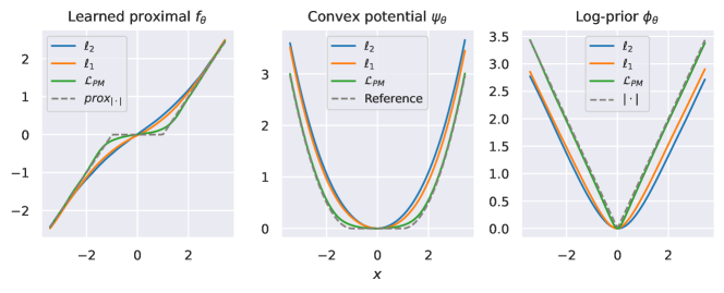
Figure 2: The proximal operator $f_{\theta}$, convex potential $\psi_{\theta}$, and log-prior $\phi_{\theta}$ learned by LPN via different losses: the squared $\ell_{2}$ loss, $\ell_{1}$ loss, and the proposed proximal matching loss $\mathcal{L}_{PM}$. The ground-truth data distribution is the Laplacian $p(x)=\tfrac{1}{2}\exp(-|x|)$, with log-prior $-\log p(x)=|x|-\log(\tfrac{1}{2})$. The gray dashed line shows the ground-truth for each case.

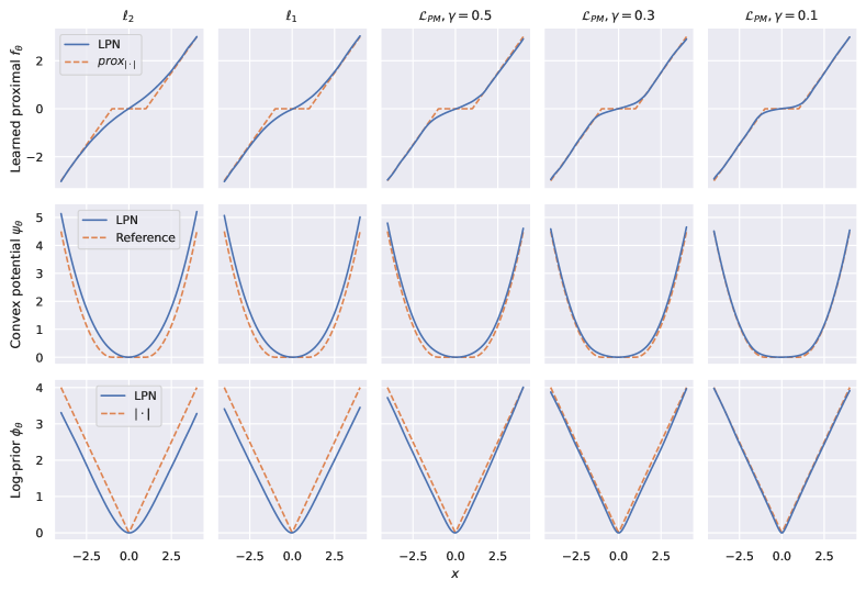
Figure 6: The proximal operator $f_{\theta}$, convex potential $\psi_{\theta}$, and log-prior $\phi_{\theta}$ learned by LPN via different losses: the square $\ell_{2}$ loss, $\ell_{1}$ loss, and the proposed proximal matching loss $\mathcal{L}_{PM}$ with different $\gamma\in\{0.5,0.3,0.1\}$. The ground-truth data distribution is the Laplacian $p(x)=\tfrac{1}{2}\exp(-|x|)$, with log-prior $-\log p(x)=|x|-\log(\tfrac{1}{2})$. With proximal matching loss, the learned proximal $f_{\theta}$ progressively approaches the ground-truth $\operatorname{prox}_{|\cdot|}$ as $\gamma$ shrinks from $0.5$ to $0.1$.

As seen in Figure 2, when using either the $\ell_{2}$ or $\ell_{1}$ loss, the learned prox differs from the correct soft-thresholding function. Indeed, verifying our analysis in Section 3.1, these losses yield the conditional mean and median, respectively, rather than the conditional mode. When we switch to the proximal matching loss $\mathcal{L}_{PM}$, the learned proximal matches much more closely the ground-truth soft-thresholding function, corroborating our theoretical analysis in Theorem 3.1 and showcasing the importance of proximal matching loss. The third panel in Figure 2 further depicts the learned log-prior $\phi_{\theta}$ associated with each LPN $f_{\theta}$, computed using the prior estimation algorithm in Section 3. These results validate the prior estimation algorithm and further demonstrate the necessity of proximal matching loss: $\phi_{\theta}$ does not match the ground-truth log-prior $|\cdot|$ for $\ell_{2}$ and $\ell_{1}$ losses, but converges to the correct data prior with $\mathcal{L}_{PM}$. The results of different $\gamma$ are included in Section G.1, Figure 6. Additionally, note that we normalize the offset of learned priors by setting the minimum value to $0$ for visualization. The absolute value of the learned log-prior $\phi_{\theta}$ is arbitrary (since we are learning the proximal operator of the log-prior, and the same prox corresponds to multiple “primitive” functions that differ by an additive constant) and, as a result, their offsets can differ. In other words, LPN is only able to learn the relative density of the distribution due to the intrinsic scaling symmetry of the proximal operator.

Learning a prior for MNIST

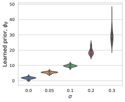
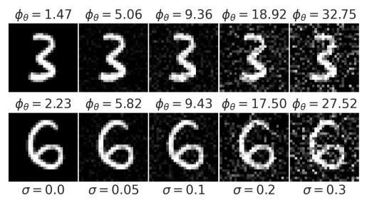
(a) Learned priors at images corrupted by additive Gaussian noise with standard deviation $\sigma$.

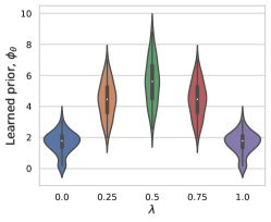
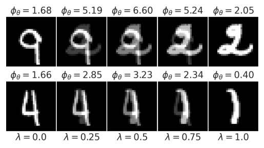
(b) Learned priors at convex combination of two images $(1-\lambda)\mathbf{x}+\lambda\mathbf{x}^{\prime}$.

Figure 3: The log-prior $\phi_{\theta}$ learned by LPN on MNIST, evaluated at images with various perturbation types and to different degrees: (a) additive Gaussian noise and (b) convex combination between two images. Left: the prior computed over 100 test images. Right: the prior $\phi_{\theta}$ evaluated at individual examples.

Next, we train an LPN on MNIST, attempting to learn a general restoration method for hand-written digits – and through it, a prior of the data. For images, we implement the LPN with convolution layers; see Section E.2 for more details. Once the model is learned, we evaluate the obtained prior on a series of inputs with different types and degrees of perturbations in order to gauge how such modifications to the data are reflected by the learned prior. Figure 3(a) visualizes the change of prior $\phi_{\theta}$ after adding increasing levels of Gaussian noise. As expected, as the noise level increases, the values reported by the log-prior also increases, reflecting that they are less likely according to the true distribution of the real images.

The lower likelihood upon perturbations of the sames is general. We depict examples with image blur in Section G.2, and also present a study that depicts the non-convexity of the log-prior in Figure 3(b): we evaluate the learned prior at the convex combination of two samples, $\lambda\mathbf{x}+(1-\lambda)\mathbf{x}^{\prime}$ of two testing images $\mathbf{x}$ and $\mathbf{x}^{\prime}$, with $\lambda\in[0,1]$. As depicted in Figure 3(b), as $\lambda$ goes from $0$ to $1$, the prior first increases then decreases, exhibiting a nonconvex shape. This is natural, since the convex combination of two images no longer resembles a natural image, hence the true prior should indeed be nonconvex. As we see, LPN can correctly learn such nonconvexity in the prior, while existing approaches using convex priors, either hand-crafted tikhonov1977solutions,rudin1992nonlinear,mallat1999wavelet,beck2009fast,elad2006image,chambolle2011first or data-driven mukherjee2020learned,cohen2021has, are suboptimal by not faithfully capturing the true prior. All these results collectively show that LPN can learn a good approximation of the prior of images from data samples, and the learned prior either recovers the correct primitive when this is known, or provides a prior that coincides with human preference of natural, realistic images. With this at hand, we now move to address more challenging inverse problems.

5.2 Solving inverse problems with LPN

CelebA

We now showcase the capability of LPN for solving realistic inverse problems. We begin by training an LPN on the CelebA dataset, and employ the Plug-and-Play methodology (PnP-ADMM) for deblurring. We compare with state-of-the-art PnP approaches: PnP-BM3D venkatakrishnan2013plug, which uses the BM3D denoiser dabov2007image, and PnP-DnCNN zhang2021plug, which uses the denoising CNN zhang2017beyond. As shown in Table 1, LPN uniformly outperforms other approaches across all blur degrees, noise levels and metrics (PSNR and SSIM) considered. As visualized in Figure 4, our method significantly improves the quality of the blurred image, demonstrating the effectiveness of the learned prior. Compared to the baseline PnP-BM3D, LPN produces sharper results with more high-frequency details. LPN achieves competitive performance with the state-of-the-art deep-learning-based DnCNN, while allowing for the evaluation of the obtained prior – which is not possible in any of the other cases.

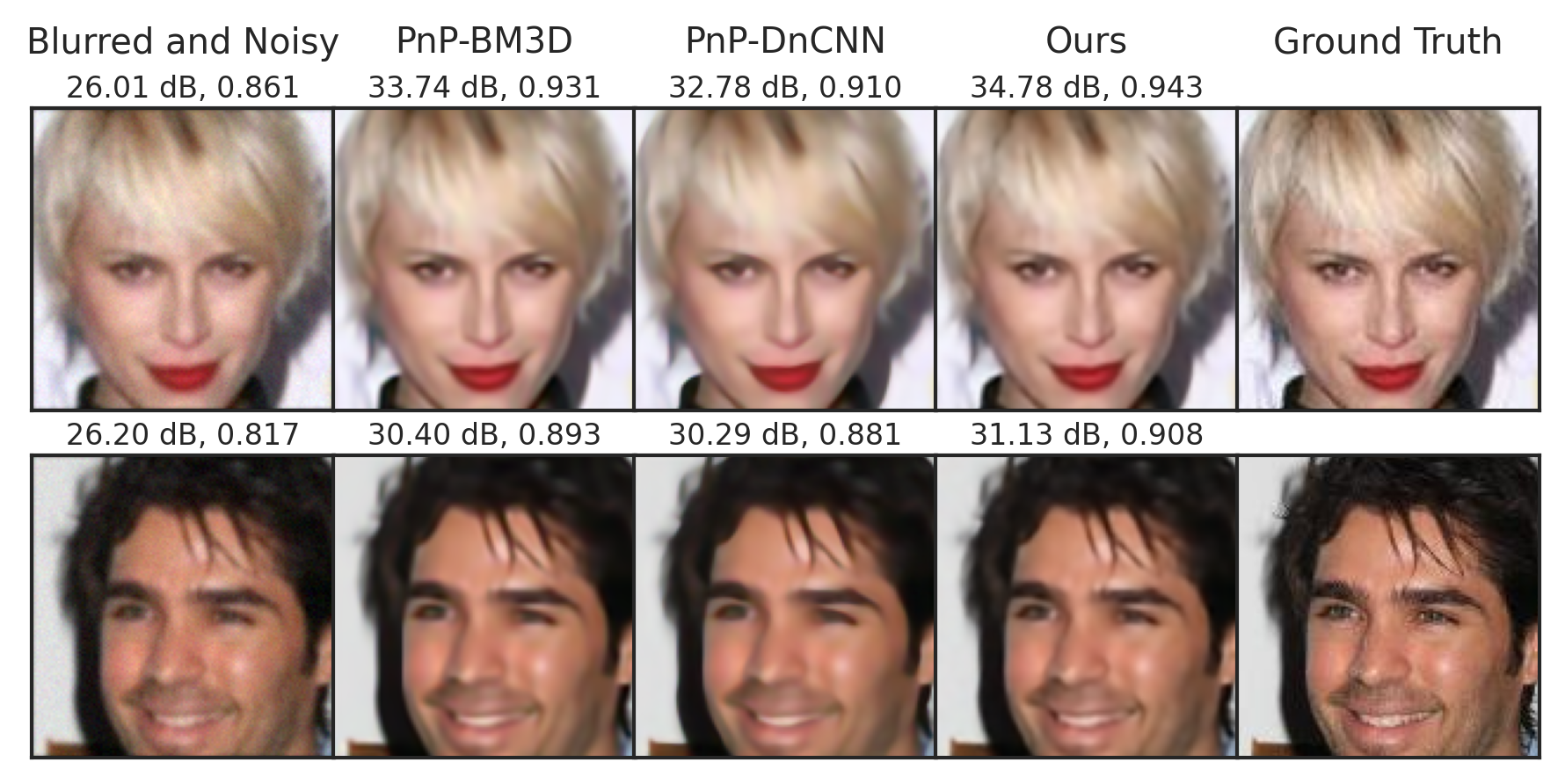
(a) $\sigma_{blur}=1.0,\sigma_{noise}=0.02$.

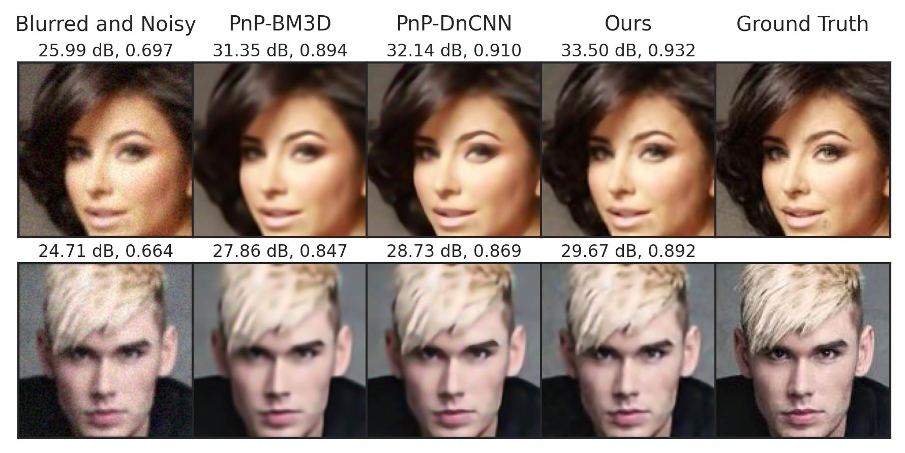
(b) $\sigma_{blur}=1.0,\sigma_{noise}=0.04$.

Figure 4: Deblurring results on CelebA using ADMM-based Plug-and-Play with different denoiser methods (BM3D venkatakrishnan2013plug, DnCNN zhang2021plug, and our LPN), for Gaussian blur kernel standard deviation $\sigma_{blur}$ and noise standard deviation $\sigma_{noise}$. PSNR and SSIM are presented above each prediction (see full numerical results in Table 1).

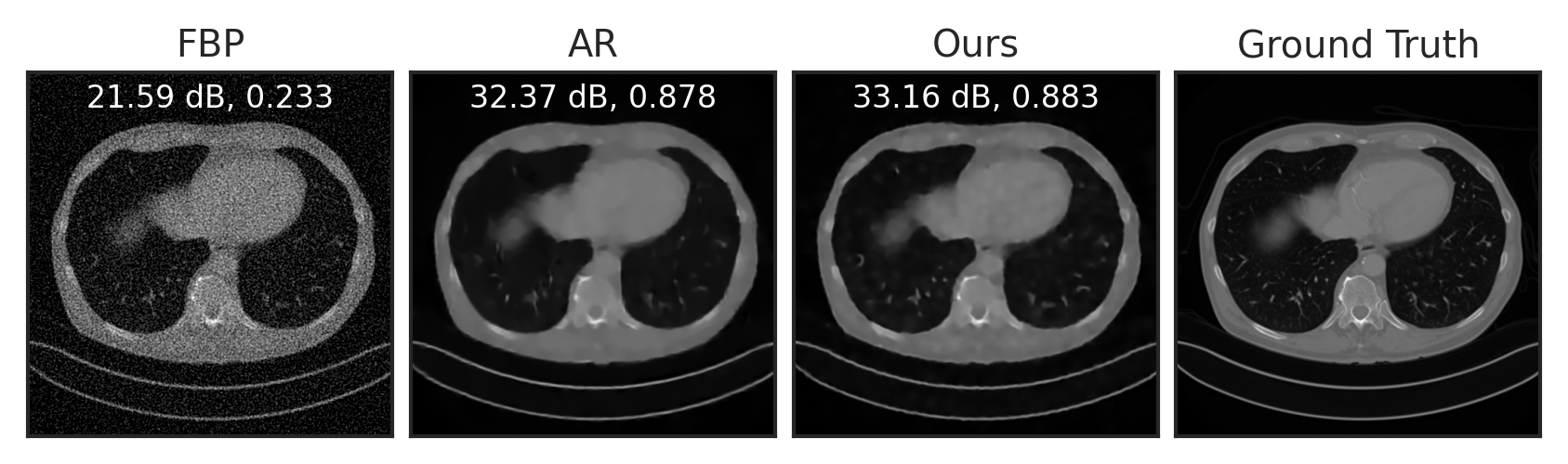
(a) Sparse-view tomographic reconstruction.

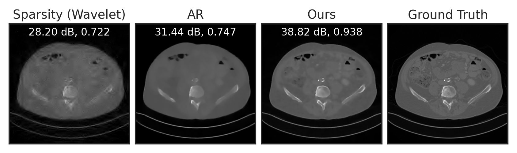
(b) Compressed sensing (compression rate $=1/16$).

Figure 5: Results of LPN for inverse problems on the Mayo-CT dataset on two examples. For sparse-view tomographic reconstruction (a) we compare with the baseline filtered back-projection (FBP) willemink2019evolution and the learned adversarial regularizer (AR) lunz2018adversarial approach. For compressed sensing (b) we compare with the baseline Wavelet sparsity regularized approach and AR. See full numerical results in Table 2.

Table 1: Numerical results on deblurring on CelebA, computed over 20 test images.

METHOD	$\sigma_{blur}=1,\,\sigma_{noise}=.02$		$\sigma_{blur}=1,\,\sigma_{noise}=.04$		$\sigma_{blur}=2,\,\sigma_{noise}=.02$		$\sigma_{blur}=2,\,\sigma_{noise}=.04$
	PSNR($\uparrow$)	SSIM($\uparrow$)	PSNR($\uparrow$)	SSIM($\uparrow$)	PSNR($\uparrow$)	SSIM($\uparrow$)	PSNR($\uparrow$)	SSIM($\uparrow$)
Blurred and Noisy	27.0 $\pm$ 1.6	.80 $\pm$ .03	24.9 $\pm$ 1.0	.63 $\pm$ .05	24.0 $\pm$ 1.7	.69 $\pm$ .04	22.8 $\pm$ 1.3	.54 $\pm$ .04
PnP-BM3D venkatakrishnan2013plug	31.0 $\pm$ 2.7	.88 $\pm$ .04	29.5 $\pm$ 2.2	.84 $\pm$ .05	28.5 $\pm$ 2.2	.82 $\pm$ .05	27.6 $\pm$ 2.0	.79 $\pm$ .05
PnP-DnCNN zhang2021plug	30.7 $\pm$ 2.5	.87 $\pm$ .04	30.3 $\pm$ 2.2	.86 $\pm$ .04	28.2 $\pm$ 2.0	.80 $\pm$ .05	28.0 $\pm$ 2.0	.80 $\pm$ .05
Ours	31.7 $\pm$ 2.9	.90 $\pm$ .04	31.1 $\pm$ 2.5	.89 $\pm$ .04	28.8 $\pm$ 2.2	.83 $\pm$ .05	28.5 $\pm$ 2.1	.82 $\pm$ .05

Mayo-CT

We train LPN on the public Mayo-CT dataset mccollough2016tu of Computed Tomography images, and evaluate it for two inverse tasks: sparse-view CT reconstruction and compressed sensing. For sparse-view CT reconstruction, we compare with the baseline filtered back-projection (FBP) approach willemink2019evolution, the adversarial regularizer (AR) lunz2018adversarial, a learning-based approach with explicit regularizer, and the improved, unrolling-based AR (UAR) mukherjee2021end. UAR is trained to solve the inverse problem for a specific measurement operator (i.e. task-specific), while both AR and LPN are generic regularizers that are applicable to any forward operator (i.e. task-agnostic). In other words, the comparison with UAR is not completely fair (as it is a task-specific method), but we include it here for comparison.

Table 2: Numerical results for inverse problems on Mayo-CT, computed over 128 test images.

METHOD	PSNR ($\uparrow$)	SSIM ($\uparrow$)
Tomographic reconstruction
FBP	21.29	.203
Operator-agnostic
AR lunz2018adversarial	33.48	.890
Ours	34.14	.891
Operator-specific
UAR mukherjee2021end	34.76	.897
Compressed sensing (compression rate $=1/16$)
Sparsity (Wavelet)	26.54	.666
AR lunz2018adversarial	29.71	.712
Ours	38.03	.919
Compressed sensing (compression rate $=1/4$)
Sparsity (Wavelet)	36.80	.921
AR lunz2018adversarial	37.94	.920
Ours	44.05	.973

Following Lunz et al. [62], we simulate CT sinograms using a parallel-beam geometry with 200 angles and 400 detectors, with an undersampling rate of $\frac{200\times 400}{512^{2}}\approx 30\%$. See Section E.4 for experimental details. As visualized in Figure 5(a), compared to the baseline FBP, LPN can significantly reduce noise in the reconstruction. Compared to AR, LPN result is slightly sharper, with higher PNSR. The numerical results in Table 2 show that our method significantly improves over the baseline FBP, outperforms the unsupervised counterpart AR, and performs just slightly worse than the supervised approach UAR – without even having had access to the used forward operator. Figure 5(b) and Table 2 show compressed sensing results with compression rates of $\frac{1}{4}$ and $\frac{1}{16}$. LPN significantly outperforms the baseline and AR, demonstrating much better generalizability to different forward operators and inverse problems.

6 Conclusion

The learned proximal networks presented in this paper form a class of neural networks that guarantees to parameterize proximal operators. We showed how the “primitive” function of the proximal operator parameterized by an LPN can be recovered, allowing explicit characterization of the prior learned from data. Furthermore, via proximal matching, LPN can learn the true prox of the log-prior of an unknown distribution from only i.i.d. samples. When used to solve general inverse problems, LPN achieves state-of-the-art results while providing more interpretability by explicit characterization of the (nonconvex) prior, with convergence guarantees. The ability to not only provide unsupervised models for general inverse problems but, chiefly, to characterize the priors learned from data open exciting new research questions of uncertainty quantification angelopoulos2022image,teneggi2023trust,sun2021deep, sampling feng2023score,chung2022diffusion,Kawar2022-hu,Kawar2021-eq,Kadkhodaie2021-kh,feng2023score, equivariant learning chen2023imaging,chen2021equivariant,chen2022robust, learning without ground-truth tachella2023sensing,tachella2022unsupervised,gao2023image, and robustness jalal2021robust,darestani2021measuring, all of which constitute matter of ongoing work.

Appendix A Related Works

Deep Unrolling

In addition to Plug-and-Play, deep unrolling is another approach using deep neural networks to replace proximal operators for solving inverse problems. Similar to PnP, the deep unrolling model is parameterized by an unrolled iterative algorithm, with certain (proximal) steps replaced by deep neural nets. In contrast to PnP, the unrolling model is trained in an end-to-end fashion by paired data of ground truth and corresponding measurements from specific forward operators. Truncated deep unrolling methods unfold the algorithm for a fixed number of steps gregor2010learning,adler2010shrinkage,liu2018alista,aggarwal2018modl,adler2018learned,zhang2020deep,Monga2021-hb,gilton2019neumann,tolooshams2023unrolled,Kobler2017-wr,chen2022learning,Mardani2018-rc, sulam2019multi, while infinite-step models have been recently developed based on deep equilibrium learning gilton2021deep,liu2022online,zou2023deep. In future work, LPN can improve the performance and interpretability of deep unrolling methods in e.g., medical applications lai2020learned,fang2023deepsti,shenoy2023unrolled or in cases that demand the analysis of robustness sulam2020adversarial. The end-to-end supervision in unrolling can also help increase the performance of LPN-based methods for inverse problems in general.

Explicit Regularizer

A series of works have been dedicated to designing explicit data-driven regularizer for inverse problems, such as RED romano2017little, AR lunz2018adversarial, ACR mukherjee2020learned, UAR mukherjee2021end and others cohen2021has,zou2023deep. Our work contributes a new angle to this field, by learning a proximal operator for the log-prior and recovering the prior from the learned proximal.

Gradient Denoiser

Gradient step (GS) denoisers cohen2021has,hurault2022gradient,hurault2022proximal are a cluster of recent approaches that parameterize a denoiser via the gradient map of a neural network. Although these works share similarities to our LPN, there are a few key differences.

1. Parameterization. In GS denoisers, the denoiser is parameterized by a gradient descent step: $f=\mathop{\mathrm{Id}}-\nabla g$, where $\mathop{\mathrm{Id}}$ represents the identity operator, and $g$ is a scalar-valued function that is parameterized directly by a neural network cohen2021has, or defined implicitly by a network $N:\mathbb{R}^{n}\rightarrow\mathbb{R}^{n}$: $g(\mathbf{y})=\frac{1}{2}\|\mathbf{y}-N(\mathbf{y})\|_{2}^{2}$ hurault2022gradient,hurault2022proximal. Cohen et al. [26] also experiment with a denoiser architecture analogous to our LPN architecture, but find its denoising performance to be inferior to the GS denoiser (we will discuss this further in the final bullet below). In order to have accompanying convergence guarantees when used in PnP schemes, these GS parameterizations demand special structures on the learned denoiser—in particular, Lipschitz constraints on $\nabla g$—which can be challenging to enforce in practice.

2. Proximal operator guarantee. The GS denoisers in Cohen et al. [26], Hurault et al. [46] are not a priori guaranteed to be proximal operators. Hurault et al. [47] proposed a way to guarantee the GS denoiser to be a proximal operator by limiting the Lipschitz constant of $\nabla g$, also exploiting the characterization of Gribonval and Nikolova [43]. However, as a result, their denoiser necessarily has a bounded Lipschitz constant, even within the support of the data distribution, limiting the generality and universality of the proximals that can be approximated. On the other hand, LPNs could parameterize any continuous proximal operator on a compact domain given universality of ICNN Huang2021-ds.

3. Training. All GS denoiser methods used the conventional $\ell_{2}$ loss for training. We propose the proximal matching loss and show that it is essential for the network to learn the correct proximal operator of the log-prior of data distribution. Indeed, we attribute the inferior performance of the ICNN-based architecture that Cohen et al. [26] experiment with, which is analogous to our LPN, to the fact that their experiments train this architecture on MMSE-based denoising, where “regression to the mean” on multimodal and nonlinear natural image data hinders performance (see, e.g., Delbracio and Milanfar [31] in this connection). The key insight that powers our successful application of LPNs in experiments is the proximal matching training framework, which allows us to make full use of the constrained capacity of the LPN in representing highly expressive proximal operators (corresponding to (nearly) maximum a-posteriori estimators for data distributions).

Appendix B Additional Theorems

B.1 Learning via proximal matching (discrete case)

Theorem B.1 (Learning via Proximal Matching (Discrete Case)).

Consider a signal $\mathbf{x}\sim P(\mathbf{x})$, with $P(\mathbf{x})$ a discrete distribution, and a noisy observation $\mathbf{y}=\mathbf{x}+\sigma\bm{\varepsilon}$, where $\bm{\varepsilon}\sim\mathcal{N}(0,\mathbf{I})$ and $\sigma>0$. Let $m_{\gamma}(x):\mathbb{R}\to\mathbb{R}$ be defined by $m_{\gamma}(x)=1-\exp\left(-\frac{x^{2}}{\gamma^{2}}\right)$ . Consider the optimization problem

$$f^{*}=\operatorname*{argmin}_{f\ \mathrm{measurable}}\lim_{\gamma\searrow 0}\mathbb{E}_{\mathbf{x},\mathbf{y}}\left[m_{\gamma}\left(\|f(\mathbf{y})-\mathbf{x}\|_{2}\right)\right].$$

Then, almost surely (i.e., for almost all $\mathbf{y}$), $f^{*}(\mathbf{y})=\operatorname*{argmax}_{\mathbf{c}}P(\mathbf{x}=\mathbf{c}\mid\mathbf{y}).$

The proof is deferred to Section C.3.

Appendix C Proofs

In this section, we include the proofs for the results presented in this paper.

C.1 Proof of Proposition 2

Proof.

By Amos et al. [4, Proposition 1], $\psi_{\theta}$ is convex. Since the activation $g$ is differentiable, $\psi_{\theta}$ is also differentiable. Hence, $f_{\theta}=\nabla\psi_{\theta}$ is the gradient of a convex function. Thus, by Proposition 1, $f_{\theta}$ is a proximal operator of a function. ∎

C.2 Proof of Theorem 3.1

Proof.

First, note by linearity of the expectation that for any measurable $f$, one has

$$\lim_{\gamma\searrow 0}\mathbb{E}_{\mathbf{x},\mathbf{y}}\left[m_{\gamma}\left(\|f(\mathbf{y})-\mathbf{x}\|_{2}\right)\right]=1-\lim_{\gamma\searrow 0}\mathbb{E}_{\mathbf{x},\mathbf{y}}\left[\varphi_{\gamma^{2}/2}(f(\mathbf{y})-\mathbf{x})\right],$$ (C.1)

where $\varphi_{\gamma^{2}/2}$ denotes the density of an isotropic Gaussian random variable with mean zero and variance $\gamma^{2}/2$. Because $p(\mathbf{x})$ is a continuous density with respect to the Lebesgue measure $d\mathbf{x}$, by Gaussian conditioning, we have that the conditional distribution of $\mathbf{x}$ given $\mathbf{y}$ admits a density $p_{\mathbf{x}\mid\mathbf{y}}$ with respect to $d\mathbf{x}$ as well. Taking conditional expectations, we have

$$\lim_{\gamma\searrow 0}\mathbb{E}_{\mathbf{x},\mathbf{y}}\left[\varphi_{\gamma^{2}/2}(f(\mathbf{y})-\mathbf{x})\right]=\lim_{\gamma\searrow 0}\mathbb{E}_{\mathbf{y}}\mathbb{E}_{\mathbf{x}\mid\mathbf{y}}\left[\varphi_{\gamma^{2}/2}(f(\mathbf{y})-\mathbf{x})\right].$$ (C.2)

From here, we can state the intuition for the remaining portion of the proof. Intuitively, because the Gaussian density $\varphi_{\sigma^{2}/2}$ concentrates more and more at zero as $\gamma\searrow 0$, and meanwhile is nevertheless a probability density for every $\gamma>0$, the inner expectation over $\mathbf{x}\mid\mathbf{y}$ leads to simply replacing the integrand with its value at $\mathbf{x}=f(\mathbf{y})$; the integrand is of course the conditional density of $\mathbf{x}$ given $\mathbf{y}$, and from here it is straightforward to argue that this leads the optimal $f$ to be (almost surely) the conditional maximum a posteriori (MAP) estimate, under our regularity assumptions on $p(\mathbf{x})$.

To make this intuitive argument rigorous, we need to translate our regularity assumptions on $p(\mathbf{x})$ into regularity of $p_{\mathbf{x}\mid\mathbf{y}}$, interchange the $\gamma$ limit in C.2 with the expectation over $\mathbf{y}$, and instantiate a rigorous analogue of the heuristic “concentration” argument. First, we have by Bayes’ rule and Gaussian conditioning

$$p_{\mathbf{x}\mid\mathbf{y}}(\mathbf{x})=\frac{\varphi_{\sigma^{2}}(\mathbf{y}-\mathbf{x})p(\mathbf{x})}{(\varphi_{\sigma^{2}}\mathbin{\ast}p)(\mathbf{y}),}$$

where $\mathbin{\ast}$ denotes convolution of densities; the denominator is the density of $\mathbf{y}$, and it satisfies $\varphi_{\sigma^{2}}\mathbin{\ast}p>0$ since $\varphi_{\sigma^{2}}>0$. In particular, this implies that $p_{\mathbf{x}\mid\mathbf{y}}$ is a continuous function of $(\mathbf{x},\mathbf{y})$, because $p(\mathbf{x})$ is continuous by assumption. We can then write, by the definition of convolution,

$$\mathbb{E}_{\mathbf{x}\mid\mathbf{y}}\left[\varphi_{\gamma^{2}/2}(f(\mathbf{y})-\mathbf{x})\right]=\varphi_{\gamma^{2}/2}\ast p_{\mathbf{x}\mid\mathbf{y}}(f(\mathbf{y})),$$

so following C.2, we have

$$\lim_{\gamma\searrow 0}\mathbb{E}_{\mathbf{x},\mathbf{y}}\left[\varphi_{\gamma^{2}/2}(f(\mathbf{y})-\mathbf{x})\right]=\lim_{\gamma\searrow 0}\mathbb{E}_{\mathbf{y}}\left[\varphi_{\gamma^{2}/2}\ast p_{\mathbf{x}\mid\mathbf{y}}(f(\mathbf{y}))\right].$$ (C.3)

We are going to argue that the limit can be moved inside the expectation in C.3 momentarily; for the moment, we consider the quantity that results after moving the limit inside the expectation. To treat this term, we apply a standard approximation to the identity argument to evaluate the limit of the preceding expression. [Ch. 3, Example 3]Stein2005-io implies that the densities $\varphi_{\gamma^{2}/2}$ constitute an approximation to the identity as $\gamma\to 0$, and because $p_{\mathbf{x}\mid\mathbf{y}}$ is continuous, we can then apply [Ch. 3, Theorem 2.1]Stein2005-io to obtain that

$$\lim_{\gamma\searrow 0}\varphi_{\gamma^{2}/2}\ast p_{\mathbf{x}\mid\mathbf{y}}(f(\mathbf{y}))=p_{\mathbf{x}\mid\mathbf{y}}(f(\mathbf{y})).$$

In particular, after justifying the interchange of limit and expectation in C.3, we will have shown, by following our manipulations from C.1, that

$$\lim_{\gamma\searrow 0}\mathbb{E}_{\mathbf{x},\mathbf{y}}\left[m_{\gamma}\left(\|f(\mathbf{y})-\mathbf{x}\|_{2}\right)\right]=1-\mathbb{E}_{\mathbf{y}}\left[p_{\mathbf{x}\mid\mathbf{y}}(f(\mathbf{y}))\right].$$ (C.4)

We will proceed to conclude the proof from this expression, and justify the limit-expectation interchange at the end of the proof. The problem at hand is equivalent to the problem

$$\operatorname*{argmax}_{f\ \mathrm{measurable}}\mathbb{E}_{\mathbf{y}}\left[p_{\mathbf{x}\mid\mathbf{y}}(f(\mathbf{y}))\right].$$

Writing the expectation as an integral, we have by Bayes’ rule as above

$$\mathbb{E}_{\mathbf{y}}\left[p_{\mathbf{x}\mid\mathbf{y}}(f(\mathbf{y}))\right]=\int_{\mathbb{R}^{d}}\varphi_{\sigma^{2}}(\mathbf{y}-f(\mathbf{y}))p(f(\mathbf{y}))d\mathbf{y}.$$

Let us define an auxiliary function $g:\mathbb{R}^{d}\times\mathbb{R}^{d}\to\mathbb{R}$ by $g(\mathbf{x},\mathbf{y})=\varphi_{\sigma^{2}}(\mathbf{y}-\mathbf{x})p(\mathbf{x})$. Then

$$\mathbb{E}_{\mathbf{y}}\left[p_{\mathbf{x}\mid\mathbf{y}}(f(\mathbf{y}))\right]=\int_{\mathbb{R}^{d}}g(f(\mathbf{y}),\mathbf{y})d\mathbf{y},$$

and moreover, for every $\mathbf{y}$, $g(\,\cdot\,,\mathbf{y})$ is continuous and compactly supported, by continuity and boundedness of the Gaussian density and the assumption that $p(\mathbf{x})$ is continuous and the random variable $\mathbf{x}\sim p(\mathbf{x})$ is bounded. We have for any measurable $f$

$$g(f(\mathbf{y}),\mathbf{y})\leq\max_{\mathbf{x}\in\mathbb{R}^{d}}g(\mathbf{x},\mathbf{y}).$$ (C.5)

Our aim is thus to argue that there is a choice of measurable $f$ such that the preceding bound can be made tight; this will imply that any measurable $f$ maximizing the objective $\mathbb{E}_{\mathbf{y}}[p_{\mathbf{x}\mid\mathbf{y}}(f(\mathbf{y}))]$ satisfies $g(f(\mathbf{y}),\mathbf{y})=\max_{\mathbf{x}\in\mathbb{R}^{d}}g(\mathbf{x},\mathbf{y})$ almost surely, or equivalently that $f(\mathbf{y})\in\operatorname*{argmax}_{\mathbf{x}\in\mathbb{R}^{d}}g(\mathbf{x},\mathbf{y})$ almost surely. The claim will then follow, because $\operatorname*{argmax}_{\mathbf{x}\in\mathbb{R}^{d}}g(\mathbf{x},\mathbf{y})=\operatorname*{argmax}_{\mathbf{x}\in\mathbb{R}^{d}}p_{\mathbf{x}\mid\mathbf{y}}(\mathbf{x})$.

To this end, define $h(\mathbf{y})=\max_{\mathbf{x}\in\mathbb{R}^{d}}g(\mathbf{x},\mathbf{y})$. Then by the Weierstrass theorem, $h$ is finite-valued, and for every $\mathbf{y}$ there exists some $\mathbf{c}\in\mathbb{R}^{d}$ such that $h(\mathbf{y})=g(\mathbf{c},\mathbf{y})$. Because $g$ is continuous, it then follows from Rockafellar and Wets [74, Theorem 1.17(c)] that $h$ is continuous. Moreover, because $g$ is continuous and for every $\mathbf{y}$, $g(\,\cdot\,,\mathbf{y})$ is compactly supported, $g$ is in particular level-bounded in $\mathbf{x}$ locally uniformly in $\mathbf{y}$ in the sense of Rockafellar and Wets [74, Definition 1.16], and it follows that the set-valued mapping $\mathbf{y}\mapsto\operatorname*{argmax}_{\mathbf{x}}g(\mathbf{x},\mathbf{y}):\mathbb{R}^{d}\rightrightarrows\mathbb{R}^{d}$ is compact-valued, by the Weierstrass theorem, and outer semicontinuous relative to $\mathbb{R}^{d}$, by Rockafellar and Wets [74, Example 5.22]. Applying Rockafellar and Wets [74, Exercise 14.9, Corollary 14.6], we conclude that the set-valued mapping $\mathbf{y}\mapsto\operatorname*{argmax}_{\mathbf{x}}g(\mathbf{x},\mathbf{y})$ is measurable, and that in particular there exists a measurable function $f^{*}:\mathbb{R}^{d}\to\mathbb{R}^{d}$ such that $f^{*}(\mathbf{y})\in\operatorname*{argmax}_{\mathbf{x}}g(\mathbf{x},\mathbf{y})$ for every $\mathbf{y}\in\mathbb{R}^{d}$. Thus, there is a measurable $f$ attaining the bound in C.5, and the claim follows after we can justify the preceding interchange of limit and expectation.

To justify the interchange of limit and expectation, we will apply the dominated convergence theorem, which requires us to show an integrable (with respect to the density of $\mathbf{y}$) upper bound for the function $\mathbf{y}\mapsto\mathbb{E}_{\mathbf{x}\mid\mathbf{y}}[\varphi_{\gamma^{2}/2}(f(\mathbf{y})-\mathbf{x})]$. For this, we calculate

$$\mathbb{E}_{\mathbf{x}\mid\mathbf{y}}\left[\varphi_{\gamma^{2}/2}(f(\mathbf{y})-\mathbf{x})\right] =\frac{1}{(\varphi_{\sigma^{2}}\ast p)(\mathbf{y})}\int_{\mathbb{R}^{d}}\varphi_{\sigma^{2}}(\mathbf{y}-\mathbf{x})p(\mathbf{x})\varphi_{\gamma^{2}/2}(f(\mathbf{y})-\mathbf{x})d\mathbf{x}$$

$$\leq\frac{1}{(\varphi_{\sigma^{2}}\ast p)(\mathbf{y})}\left[\sup_{\mathbf{x}}\,\varphi_{\sigma^{2}}(\mathbf{y}-\mathbf{x})p(\mathbf{x})\right]\int_{\mathbb{R}^{d}}\varphi_{\gamma^{2}/2}(f(\mathbf{y})-\mathbf{x})d\mathbf{x}$$

$$=\frac{1}{(\varphi_{\sigma^{2}}\ast p)(\mathbf{y})}\left[\sup_{\mathbf{x}}\,\varphi_{\sigma^{2}}(\mathbf{y}-\mathbf{x})p(\mathbf{x})\right],$$

by Hölder’s inequality and the fact that $\varphi_{\gamma^{2}/2}$ is a probability density. Because the random variable $\mathbf{x}\sim p(\mathbf{x})$ is assumed bounded, the density $p(\mathbf{x})$ has compact support, and the density $p(\mathbf{x})$ is assumed continuous, so there exists $R>0$ such that if $\|\mathbf{x}\|_{2}>R$ then $p(\mathbf{x})=0$, and $M>0$ such that $p(\mathbf{x})\leq M$. We then have

$$\sup_{\mathbf{x}}\,\varphi_{\sigma^{2}}(\mathbf{y}-\mathbf{x})p(\mathbf{x})\leq M\sup_{\mathbf{x}}\,\varphi_{\sigma^{2}}(\mathbf{y}-\mathbf{x})\mathds{1}_{\|\mathbf{x}\|_{2}\leq R}.$$

This means that the supremum can attain a nonzero value only on points where $\|\mathbf{x}\|_{2}\leq R$. On the other hand, for every $\mathbf{y}$ with $\|\mathbf{y}\|_{2}\geq 2R$, whenever $\|\mathbf{x}\|_{2}\leq R$ the triangle inequality implies $\|\mathbf{y}-\mathbf{x}\|_{2}\geq\|\mathbf{y}\|_{2}-\|\mathbf{x}\|_{2}\geq\tfrac{1}{2}\|\mathbf{y}\|_{2}$. Because the Gaussian density $\varphi_{\sigma^{2}}$ is a radial function, we conclude that if $\|\mathbf{y}\|_{2}\geq 2R$, one has

$$\sup_{\mathbf{x}}\,\varphi_{\sigma^{2}}(\mathbf{y}-\mathbf{x})p(\mathbf{x})\leq M\varphi_{\sigma^{2}}(\mathbf{y}/2)=CM\varphi_{4\sigma^{2}}(\mathbf{y}),$$

where $C>0$ depends only on $d$. At the same time, we always have

$$\sup_{\mathbf{x}}\,\varphi_{\sigma^{2}}(\mathbf{y}-\mathbf{x})p(\mathbf{x})\leq\frac{M}{(2\pi\sigma^{2})^{d/2}}.$$

Consequently, we have the composite upper bound

$$\sup_{\mathbf{x}}\,\varphi_{\sigma^{2}}(\mathbf{y}-\mathbf{x})p(\mathbf{x})\leq\begin{cases}\tfrac{M}{(2\pi\sigma^{2})^{d/2}}&\|\mathbf{y}\|_{2}<2R\\ 2M\varphi_{4\sigma^{2}}(\mathbf{y})&\|\mathbf{y}\|_{2}\geq 2R,\end{cases}$$

and by our work above

$$\mathbb{E}_{\mathbf{x}\mid\mathbf{y}}\left[\varphi_{\gamma^{2}/2}(f(\mathbf{y})-\mathbf{x})\right]\leq\frac{1}{(\varphi_{\sigma^{2}}\ast p)(\mathbf{y})}\times\begin{cases}\tfrac{M}{(2\pi\sigma^{2})^{d/2}}&\|\mathbf{y}\|_{2}<2R\\ 2M\varphi_{4\sigma^{2}}(\mathbf{y})&\|\mathbf{y}\|_{2}\geq 2R.\end{cases}$$

Because $\varphi_{\sigma^{2}}\mathbin{\ast}p$ is the density of $\mathbf{y}$, this upper bound is sufficient to apply the dominated convergence theorem to obtain

$$\lim_{\gamma\searrow 0}\mathbb{E}_{\mathbf{x},\mathbf{y}}\left[\varphi_{\gamma^{2}/2}(f(\mathbf{y})-\mathbf{x})\right]=\mathbb{E}_{\mathbf{y}}\lim_{\gamma\searrow 0}\mathbb{E}_{\mathbf{x}\mid\mathbf{y}}\left[\varphi_{\gamma^{2}/2}(f(\mathbf{y})-\mathbf{x})\right].$$

Combining this assertion with the argument surrounding C.4, we conclude the proof.

∎

Remark (Other loss choices).

Theorem 3.1 also holds for any $m_{\gamma}$ such that $m_{\gamma}$ is uniformly (in $\gamma$) bounded above, for each $\gamma>0$ uniquely minimized at $0$, and $\sup_{x\in\mathbb{R}}m_{\gamma}(x)-m_{\gamma}(\|\mathbf{x}\|_{2})$ is an approximation to the identity as $\gamma\searrow 0$ (see [Ch. 3, §2]Stein2005-io).

C.3 Proof of Theorem B.1

Proof.

For brevity, we denote $\operatorname*{argmax}_{\mathbf{c}}P(\mathbf{x}=\mathbf{c}\mid\mathbf{y})$ by $\mathrm{MAP}[\mathbf{x}\mid\mathbf{y}]$, i.e., the maximum a posteriori estimate of $\mathbf{x}$ given $\mathbf{y}$.

First, we show that $\mathrm{MAP}[\mathbf{x}\mid\mathbf{y}]$ is unique for almost all $\mathbf{y}$.

Consider $\mathbf{y}$ such that $\mathrm{MAP}[\mathbf{x}\mid\mathbf{y}]$ is not unique. There exists $i\neq j$, such that

$$P(\mathbf{x}_{i}\mid\mathbf{y})=P(\mathbf{x}_{j}\mid\mathbf{y})$$

$$\iff p(\mathbf{y}\mid\mathbf{x}_{i})P(\mathbf{x}_{i})=p(\mathbf{y}\mid\mathbf{x}_{j})P(\mathbf{x}_{j})$$

$$\iff -\frac{1}{2}\|\mathbf{y}-\mathbf{x}_{i}\|^{2}+\sigma^{2}\log P(\mathbf{x}_{i})=-\frac{1}{2}\|\mathbf{y}-\mathbf{x}_{j}\|^{2}+\sigma^{2}\log P(\mathbf{x}_{j})$$

$$\iff \langle\mathbf{y},\frac{\mathbf{x}_{i}-\mathbf{x}_{j}}{2}\rangle=\frac{1}{2}\|\mathbf{x}_{i}\|^{2}-\frac{1}{2}\|\mathbf{x}_{j}\|^{2}-\sigma^{2}\log P(\mathbf{x}_{i})+\sigma^{2}\log P(\mathbf{x}_{j}).$$

i.e., $\mathbf{y}$ lies in a hyperplane defined by $\mathbf{x}_{i},\mathbf{x}_{j}$ (note that $\mathbf{x}_{i}\neq\mathbf{x}_{j}$). Denote the hyperplane by

$$\mathcal{H}_{i,j}:=\left\{\mathbf{y}\mid\langle\mathbf{y},\frac{\mathbf{x}_{i}-\mathbf{x}_{j}}{2}\rangle=\frac{1}{2}\|\mathbf{x}_{i}\|^{2}-\frac{1}{2}\|\mathbf{x}_{j}\|^{2}-\sigma^{2}\log P(\mathbf{x}_{i})+\sigma^{2}\log P(\mathbf{x}_{j})\right\}.$$

Consider

$$\mathcal{U}:=\cup_{i\neq j}\mathcal{H}_{i,j}.$$

We have that $\forall\mathbf{y}$ with non-unique $\mathrm{MAP}[\mathbf{x}\mid\mathbf{y}]$,

$$\exists i\neq j,\mathbf{y}\in\mathcal{H}_{i,j}$$

$$\iff \mathbf{y}\in\mathcal{U}.$$

Note that $\mathcal{U}$ has zero measure as a countable union of zero-measure sets, hence the measure of all $\mathbf{y}$ with non-unique $\mathrm{MAP}[\mathbf{x}\mid\mathbf{y}]$ is zero. Hence, for almost all $\mathbf{y}$, $\mathrm{MAP}[\mathbf{x}\mid\mathbf{y}]$ is unique.

Next, we show that for almost all $\mathbf{y}$,

$$f^{*}(\mathbf{y})=\operatorname*{argmin}_{\mathbf{c}}\mathbb{E}_{\mathbf{x}\mid\mathbf{y}}[\mathds{1}_{\mathbf{c}\neq\mathbf{x}}].$$

Note that

$$\lim_{\gamma\searrow 0}\mathbb{E}_{\mathbf{x},\mathbf{y}}\left[m_{\gamma}\left(\|f(\mathbf{y})-\mathbf{x}\|_{2}\right)\right]$$

$$= \mathbb{E}_{\mathbf{x},\mathbf{y}}\left[\lim_{\gamma\searrow 0}m_{\gamma}\left(\|f(\mathbf{y})-\mathbf{x}\|_{2}\right)\right]$$

$$= \mathbb{E}_{\mathbf{x},\mathbf{y}}\left[\mathds{1}_{\|f(\mathbf{y})-\mathbf{x}\|_{2}\neq 0}\right]$$

$$= \mathbb{E}_{\mathbf{x},\mathbf{y}}\left[\mathds{1}_{f(\mathbf{y})\neq\mathbf{x}}\right].$$

Above, the first equality uses the monotone convergence theorem. Use the law of iterated expectations,

$$\mathbb{E}_{\mathbf{x},\mathbf{y}}\left[\mathds{1}_{f(\mathbf{y})\neq\mathbf{x}}\right]=\mathbb{E}_{\mathbf{y}}\mathbb{E}_{\mathbf{x}\mid\mathbf{y}}\left[\mathds{1}_{f(\mathbf{y})\neq\mathbf{x}}\right].$$

We will use this expression to study the global minimizers of the objective. By conditioning,

$$\mathbb{E}_{\mathbf{x}\mid\mathbf{y}}\left[\mathds{1}_{f(\mathbf{y})\neq\mathbf{x}}\right]\geq\min_{\mathbf{c}}\mathbb{E}_{\mathbf{x}\mid\mathbf{y}}[\mathds{1}_{\mathbf{c}\neq\mathbf{x}}],$$

and so

$$\mathbb{E}_{\mathbf{y}}\left[\mathbb{E}_{\mathbf{x}\mid\mathbf{y}}\left[\mathds{1}_{f(\mathbf{y})\neq\mathbf{x}}\right]-\min_{\mathbf{c}}\mathbb{E}_{\mathbf{x}\mid\mathbf{y}}[\mathds{1}_{\mathbf{c}\neq\mathbf{x}}]\right]\geq 0.$$

Because $p(\mathbf{y})>0$, it follows that every global minimizer of the objective $f^{*}$ satisfies

$$\mathbb{E}_{\mathbf{x}\mid\mathbf{y}}\left[\mathds{1}_{f^{*}(\mathbf{y})\neq\mathbf{x}}\right]=\min_{\mathbf{c}}\mathbb{E}_{\mathbf{x}\mid\mathbf{y}}[\mathds{1}_{\mathbf{c}\neq\mathbf{x}}]\enspace\text{a.s.}$$

Hence, for almost all $\mathbf{y}$,

$$f^{*}(\mathbf{y})\in\operatorname*{argmin}_{\mathbf{c}}\mathbb{E}_{\mathbf{x}\mid\mathbf{y}}[\mathds{1}_{\mathbf{c}\neq\mathbf{x}}].$$

Finally, we show that $\operatorname*{argmin}_{\mathbf{c}}\mathbb{E}_{\mathbf{x}\mid\mathbf{y}}[\mathds{1}_{\mathbf{c}\neq\mathbf{x}}]=\mathrm{MAP}[\mathbf{x}\mid\mathbf{y}]$. The claim then follows from our preceding work showing that $\mathrm{MAP}[\mathbf{x}\mid\mathbf{y}]$ is almost surely unique. Consider

$$\mathbb{E}_{\mathbf{x}\mid\mathbf{y}}[\mathds{1}_{\mathbf{c}\neq\mathbf{x}}] =\sum_{i}P(\mathbf{x}_{i}\mid\mathbf{y})\mathds{1}_{\mathbf{c}\neq\mathbf{x}_{i}}$$

$$=\sum_{i}P(\mathbf{x}_{i}\mid\mathbf{y})(1-\mathds{1}_{\mathbf{c}=\mathbf{x}_{i}})$$

$$=\sum_{i}P(\mathbf{x}_{i}\mid\mathbf{y})-\sum_{\mathbf{x}_{i}=\mathbf{c}}P(\mathbf{x}_{i}\mid\mathbf{y})$$

$$=1-P(\mathbf{x}=\mathbf{c}\mid\mathbf{y}).$$

Hence,

$$\operatorname*{argmin}_{\mathbf{c}}\mathbb{E}_{\mathbf{x}\mid\mathbf{y}}[\mathds{1}_{\mathbf{c}\neq\mathbf{x}}] =\operatorname*{argmax}_{\mathbf{c}}P(\mathbf{x}=\mathbf{c}\mid\mathbf{y})$$

$$=\mathrm{MAP}[\mathbf{x}\mid\mathbf{y}].$$

∎

C.4 Proof of Theorem 4.1

We provide a proof of Theorem 4.1 under slightly more general assumptions in these appendices. The result is restated in this general setting below, as Footnote 13.

Theorem C.1.

Consider the sequence of iterates $\mathbf{x}_{k}$, $k\in\{0,1,\dots\}$, defined by Algorithm 1 run with a continuously differentiable measurement operator $A$ and a LPN $f_{\theta}$ with softplus activations, trained with $0<\alpha<1$. Assume further that the data fidelity term $h(\mathbf{x})=\tfrac{1}{2}\|\mathbf{y}-A(\mathbf{x})\|_{2}^{2}$ is definable in an o-minimal structure and has $L$-Lipschitz gradient, and that the step size satisfies $0<\eta<1/L$. Then, the iterates $\mathbf{x}_{k}$ converge to a fixed point $\mathbf{x}^{*}$ of Algorithm 1: that is, there exist $\mathbf{x}^{*}\in\mathbb{R}^{n}$ such that

$$f_{\theta}\left(\mathbf{x}^{*}-\eta\nabla h(\mathbf{x}^{*})\right)=\mathbf{x}^{*},$$ (C.6)

and $\lim_{k\to\infty}\mathbf{x}_{k}=\mathbf{x}^{*}$. Furthermore, $\mathbf{x}^{*}$ is a critical point of $h+\tfrac{1}{\eta}\phi_{\theta}$, where $\phi_{\theta}$ is the prior associated to the LPN $f_{\theta}$ (i.e., $f_{\theta}=\operatorname{prox}_{\phi_{\theta}}$).

Before proceeding to the proof, we state a few settings and results from Boţ et al. [15] that are useful for proving Footnote 13, for better readability.

Problem 1 ([Problem 1]Bot2016-mw).

Let $f:\mathbb{R}^{m}\to(-\infty,+\infty]$ be a proper, lower semicontinuous function which is bounded below and let $h:\mathbb{R}^{m}\to\mathbb{R}$ be a Fréchet differentiable function with Lipschitz continuous gradient, i.e. there exists $L_{\nabla h}\geq 0$ such that $\|\nabla h(\mathbf{x})-\nabla h(\mathbf{x}^{\prime})\|\leq L_{\nabla h}\|\mathbf{x}-\mathbf{x}^{\prime}\|$ for all $\mathbf{x},\mathbf{x}^{\prime}\in\mathbb{R}^{m}$. Consider the optimization problem

$$(P)\ \ \underset{\mathbf{x}\in\mathbb{R}^{m}}{\inf}[f(\mathbf{x})+h(\mathbf{x})].$$

Algorithm C.1 ([Algorithm 1]Bot2016-mw).

Choose $\mathbf{x}_{0},\mathbf{x}_{1}\in\mathbb{R}^{m},\underline{\alpha},\overline{\alpha}>0,\beta\geq 0$ and the sequences $(\alpha_{n})_{n\geq 1},(\beta_{n})_{n\geq 1}$ fulfilling

$$0<\underline{\alpha}\leq\alpha_{n}\leq\overline{\alpha}\ \ \forall n\geq 1$$

and

$$0\leq\beta_{n}\leq\beta\ \ \forall n\geq 1.$$

Consider the iterative scheme

$$(\forall n\geq 1)\ \mathbf{x}_{n+1}\in\operatorname*{argmin}_{\mathbf{u}\in\mathbb{R}^{m}}\{D_{F}(\mathbf{u},\mathbf{x}_{n})+\alpha_{n}\langle\mathbf{u},\nabla h(\mathbf{x}_{n})\rangle+\beta_{n}\langle\mathbf{u},\mathbf{x}_{n-1}-\mathbf{x}_{n}\rangle+\alpha_{n}f(\mathbf{u})\}.$$ (C.7)

Here, $F:\mathbb{R}^{m}\to\mathbb{R}$ is $\sigma$-strongly convex, Fréchet differentiable and $\nabla F$ is $L_{\nabla F}$-Lipschitz continuous, with $\sigma,L_{\nabla F}>0$; $D_{F}$ is the Bregman distance to $F$.

Theorem C.2 ([Theorem 13]Bot2016-mw).

In the setting of 1, choose $\underline{\alpha}$, $\overline{\alpha}$, $\beta$ satisfying

$$\sigma>\overline{\alpha}L_{\nabla_{h}}+2\beta\frac{\overline{\alpha}}{\underline{\alpha}}.$$ (C.8)

Assume that $f+h$ is coercive and that

$$H:\mathbb{R}^{m}\times\mathbb{R}^{m}\to(-\infty,+\infty],\ H(\mathbf{x},\mathbf{x}^{\prime})=(f+h)(\mathbf{x})+\frac{\beta}{2\underline{\alpha}}\|\mathbf{x}-\mathbf{x}^{\prime}\|^{2},\ \forall(\mathbf{x},\mathbf{x}^{\prime})\in\mathbb{R}^{m}\times\mathbb{R}^{m}$$

is a KL function. Let $(\mathbf{x}_{n})_{n\in\mathbb{N}}$ be a sequence generated by C.1. Then the following statements are true:

1. $\sum_{n\in\mathbb{N}}\|\mathbf{x}_{n+1}-\mathbf{x}_{n}\|<+\infty$

2. there exists $\mathbf{x}\in\operatorname{crit}(f+h)$ such that $\lim_{n\to+\infty}\mathbf{x}_{n}=\mathbf{x}$.

Now, we prove Footnote 13.

Proof of Footnote 13..

By Lemma C.4, there is a coercive function $\phi_{\theta}:\mathbb{R}^{d}\to\mathbb{R}\cup\{+\infty\}$ such that $f_{\theta}=\operatorname{prox}_{\phi_{\theta}}$. The idea of the proof is to apply Theorem C.2 to our setting; this requires us to check that Algorithm 1 maps onto C.1, and that our (implicitly-defined) objective function and parameter choices satisfy the requirements of this theorem. To this end, note that the application of $f_{\theta}$ in Algorithm 1 can be written as

$$\mathbf{x}_{k+1} =f_{\theta}\left(\mathbf{x}_{k}-\eta\nabla h(\mathbf{x}_{k})\right)$$

$$=\operatorname*{argmin}_{\mathbf{x}^{\prime}\in\mathbb{R}^{n}}\,\frac{1}{2}\left\|\mathbf{x}^{\prime}-\left(\mathbf{x}_{k}-\eta\nabla h(\mathbf{x}_{k})\right)\right\|_{2}^{2}+\phi_{\theta}(\mathbf{x}^{\prime})$$

$$=\operatorname*{argmin}_{\mathbf{x}^{\prime}\in\mathbb{R}^{n}}\,\frac{1}{2}\left\|\mathbf{x}^{\prime}-\mathbf{x}_{k}\right\|_{2}^{2}+\langle\mathbf{x}^{\prime}-\mathbf{x}_{k},\eta\nabla h(\mathbf{x}_{k})\rangle+\phi_{\theta}(\mathbf{x}^{\prime})$$

$$=\operatorname*{argmin}_{\mathbf{x}^{\prime}\in\mathbb{R}^{n}}\,\frac{1}{2}\left\|\mathbf{x}^{\prime}-\mathbf{x}_{k}\right\|_{2}^{2}+\eta\langle\mathbf{x}^{\prime},\nabla h(\mathbf{x}_{k})\rangle+\eta\cdot\frac{1}{\eta}\phi_{\theta}(\mathbf{x}^{\prime})$$

showing that Algorithm 1 corresponds to C.1 with the Bregman distance $D_{F}(\mathbf{x},\mathbf{y})=\tfrac{1}{2}\|\mathbf{x}-\mathbf{y}\|_{2}^{2}$ (and correspondingly $F(\mathbf{x})=\tfrac{1}{2}\|\mathbf{x}\|_{2}^{2}$, which satisfies $\sigma=L_{\nabla F}=1$), the momentum parameter $\beta=\beta_{n}=0$, the step size $\alpha_{n}=\overline{\alpha}=\underline{\alpha}=\eta$, and $f=\tfrac{1}{\eta}\phi_{\theta}$. In the framework of Boţ et al. [15], Algorithm 1 minimizes the implicitly-defined objective $h+\eta^{-1}\phi_{\theta}$. Moreover, one checks that our choice of constant step size $0<\eta<1/L$ verifies the necessary condition C.8, and because $h\geq 0$, coercivity of $\phi_{\theta}$ implies that $h+\eta^{-1}\phi_{\theta}$ is coercive. The final hypothesis to check, which is slightly technical, is to show that the implicit objective $h+\eta^{-1}\phi_{\theta}$ is a KL function—this suffices to apply Theorem C.2 since for Algorithm 1, the parameter $\beta$ in Theorem C.2 is zero. To this end, we make use of the fact that any proper lower-semicontinuous function definable in an “o-minimal” structure is a KL function [Theorem 4.1]Attouch2010-vs; we will argue that our objective $h+\eta^{-1}\phi_{\theta}$ is definable to conclude convergence to a critical point of $h+\eta^{-1}\phi_{\theta}$ with Theorem C.2, then show that the convergence implies the asserted fixed point convergence C.6. Because finite linear combinations of definable functions are definable and $h$ is assumed definable (see [§4.3]Attouch2010-vs: here and below, we make extensive use of the properties asserted in this section of this reference), it suffices to show that $\phi_{\theta}$ is definable. To this end, notice that the defining equation for $\phi_{\theta}$ in the $\alpha\in(0,1)$ setting, namely C.9, expresses $\phi_{\theta}$ as a finite linear combination of finite products and compositions of different functions; we will argue that each constituent function is definable.

1. $\alpha$-free LPN $\psi_{\theta}$. The definition of $\psi_{\theta}$ in Proposition 2 ensures that whenever (each coordinate function of) the elementwise activation function $g$ is definable, $\psi_{\theta}$ is definable (following the inductive argument in the proof of Lemma C.4), by the fact that finite sums and compositions of definable functions are definable [Definition 4.1]Attouch2010-vs, and that affine functions are definable. In the present setting, the softplus activation $g=\beta^{-1}\log(1+\exp(\beta x))$ is definable, because $\exp$ is definable in a certain o-minimal structure and inverses of definable functions are definable. Thus $\psi_{\theta}$ is definable.

2. Gradient of $\alpha$-free LPN $\nabla\psi_{\theta}$. This step of the proof uses the chain rule (essentially, the backpropagation algorithm to compute $\nabla\psi_{\theta}$), and the fact that finite products of definable functions remain definable. Arguing inductively (as in the inductive argument in the proof of Lemma C.4), it follows that $\nabla\psi_{\theta}$ is definable if the derivative of the activation function $g$ is definable. We calculate $g^{\prime}(x)=(1+\exp(-\beta x))^{-1}$, which is a composition of a linear function (definable), the exponential function (definable), and a rational function with nonvanishing denominator on the range of the exponential function (semialgebraic [§2.2.1]Coste2000-lw, hence definable). This shows that $\nabla\psi_{\theta}$ is definable.

3. Inverse of $\alpha$-regularized LPN $f_{\theta}^{-1}$. The map $f_{\theta}(\mathbf{x})=\nabla\psi_{\theta}(\mathbf{x})+\alpha\mathbf{x}$ is definable, as a sum of definable functions (by our work above). Because inverses of invertible definable functions are definable, and because $f_{\theta}$ is invertible (by Lemma C.4), it follows that $f_{\theta}^{-1}$ is definable.

4. Squared $\ell_{2}$ norm. This is a polynomial function, hence semialgebraic and definable.

Thus $h+\eta^{-1}\phi_{\theta}$ is definable, continuous (by Lemma C.4), and proper (as a sum of real-valued functions, again by Lemma C.4), and therefore has the KL property. We can therefore apply Theorem C.2 to conclude convergence to a critical point of $h+\eta^{-1}\phi_{\theta}$. Finally, by Lemma C.3 and the continuity of $f_{\theta}$ and $\nabla h$, we conclude convergence to a fixed point, $\mathbf{x}=f_{\theta}(\mathbf{x}-\eta\nabla h(\mathbf{x}))$, which is identical to C.6. ∎

Lemma C.3 (Convergence Implies Fixed Point Convergence).

Suppose $\mathcal{F}:\mathbb{R}^{n}\to\mathbb{R}^{n}$ is a continuous map that defines an iterative process, $\mathbf{x}_{k+1}=\mathcal{F}(\mathbf{x}_{k})$. Assume $\mathbf{x}_{k}$ converges, i.e., $\exists\ \mathbf{x}^{*}$ such that $\lim_{k\to\infty}\mathbf{x}_{k}=\mathbf{x}^{*}$. Then, $\mathbf{x}^{*}$ is a fixed point of $\mathcal{F}$, i.e., $\mathbf{x}^{*}=\mathcal{F}(\mathbf{x}^{*})$.

Proof.

$$\mathbf{x}^{*}=\lim_{k\to\infty}\mathbf{x}_{k}=\lim_{k\to\infty}\mathbf{x}_{k+1}=\lim_{k\to\infty}\mathcal{F}(\mathbf{x}_{k})=\mathcal{F}\left(\lim_{k\to\infty}\mathbf{x}_{k}\right)=\mathcal{F}(\mathbf{x}^{*}).$$

The fourth equality follows from continuity of $\mathcal{F}$. ∎

Lemma C.4 (Regularity Properties of LPNs).

Suppose $f_{\theta}$ is a LPN constructed following the recipe in Proposition 2, with softplus activations $\sigma(x)=(1/\beta)\log(1+\exp(\beta x))$, where $\beta>0$ is an arbitrary constant, and with strong convexity weight $0<\alpha<1$. Let $f_{\theta}(\mathbf{y})=\nabla\psi_{\theta}(\mathbf{y})+\alpha\mathbf{y}$ be the defining equation of the LPN. Then there is a function $\phi_{\theta}:\mathbb{R}^{n}\to\mathbb{R}\cup\{+\infty\}$ such that $f_{\theta}=\operatorname{prox}_{\phi_{\theta}}$. Moreover, we have the following regularity properties:

1. $\phi_{\theta}$ is coercive, i.e., we have $\phi_{\theta}(\mathbf{x})\to+\infty$ as $\|\mathbf{x}\|_{2}\to+\infty$.

2. $f_{\theta}:\mathbb{R}^{n}\to\mathbb{R}^{n}$ is surjective and invertible, with an inverse mapping $f_{\theta}^{-1}:\mathbb{R}^{n}\to\mathbb{R}^{n}$ which is continuous.

3. $\phi_{\theta}$ is continuously differentiable and real-valued. In particular, it holds

   $$\begin{split}\phi_{\theta}(\mathbf{x})&=(1-\alpha)\langle f^{-1}_{\theta}(\mathbf{x}),\nabla\psi_{\theta}(f^{-1}_{\theta}(\mathbf{x}))\rangle\\ &\quad+\frac{\alpha(1-\alpha)}{2}\|f^{-1}_{\theta}(\mathbf{x})\|_{2}^{2}-\tfrac{1}{2}\|\nabla\psi_{\theta}(f^{-1}_{\theta}(\mathbf{x}))\|_{2}^{2}-\psi_{\theta}(f^{-1}_{\theta}(\mathbf{x})).\end{split}$$ (C.9)

Remark.

Lemma C.4 does not, strictly speaking, require the softplus activation: the proof shows that any Lipschitz activation function with enough differentiability and slow growth at infinity, such as another smoothed verison of the ReLU activation, the GeLU, or the Swish activation, would also work.

Proof of Lemma C.4..

The main technical challenge will be to establish coercivity of $\phi_{\theta}$, which always exists as necessary, by Propositions 1 and 2. We will therefore pursue this estimate as the main line of the proof, establishing the remaining assertions in the result statement along the way.

By Proposition 2, there exists $\phi_{\theta}$ such that $f_{\theta}=\operatorname{prox}_{\phi_{\theta}}$. Now, using [Theorem 4(a)]gribonval2020characterization, for every $\mathbf{y}\in\mathbb{R}^{n}$,

$$\phi_{\theta}(f_{\theta}(\mathbf{y}))=\langle\mathbf{y},f_{\theta}(\mathbf{y})\rangle-\tfrac{1}{2}\|f_{\theta}(\mathbf{y})\|_{2}^{2}-\left(\psi_{\theta}(\mathbf{y})+\tfrac{\alpha}{2}\|\mathbf{y}\|_{2}^{2}\right).$$

Using the definition of $f_{\theta}$ and minor algebra, we rewrite this as

$$\phi_{\theta}(f_{\theta}(\mathbf{y})) =\langle\mathbf{y},\nabla\psi_{\theta}(\mathbf{y})+\alpha\mathbf{y}\rangle-\tfrac{1}{2}\|\nabla\psi_{\theta}(\mathbf{y})+\alpha\mathbf{y}\|_{2}^{2}-\left(\psi_{\theta}(\mathbf{y})+\tfrac{\alpha}{2}\|\mathbf{y}\|_{2}^{2}\right)$$

$$=(1-\alpha)\langle\mathbf{y},\nabla\psi_{\theta}(\mathbf{y})\rangle+\frac{\alpha(1-\alpha)}{2}\|\mathbf{y}\|_{2}^{2}-\tfrac{1}{2}\|\nabla\psi_{\theta}(\mathbf{y})\|_{2}^{2}-\psi_{\theta}(\mathbf{y}).$$ (C.10)

At this point, we observe that by Lemma C.5, the map $f_{\theta}:\mathbb{R}^{n}\to\mathbb{R}^{n}$ is invertible and surjective, with a continuous inverse mapping. This establishes the second assertion that we have claimed. In addition, taking inverses in C.10 implies C.9 and as a consequence the fact that $\phi_{\theta}$ is real-valued, and the fact that it is continuously differentiable on $\mathbb{R}^{n}$ is then an immediate consequence of [Corollary 6(b)]gribonval2020characterization. To conclude, it only remains to show that $\phi_{\theta}$ is coercive, which we will accomplish by lower bounding the RHS of C.10. By Lemma C.6, $\psi_{\theta}$ is $L$-Lipschitz for a constant $L>0$. Thus, we have for every $\mathbf{y}$ (by the triangle inequality)

$$|\psi_{\theta}(\mathbf{y})|\leq L\|\mathbf{y}\|_{2}+K$$

for a (finite) constant $K\in\mathbb{R}$, depending only on $\theta$. Now, the Cauchy-Schwarz inequality implies from the previous two statements (and $\|\nabla\psi_{\theta}\|_{2}\leq L$ by the Lipschitz property of $\psi_{\theta}$)

$$\phi_{\theta}(f_{\theta}(\mathbf{y})) \geq-(1-\alpha)\|\mathbf{y}\|_{2}\|\nabla\psi_{\theta}(\mathbf{y})\|_{2}+\frac{\alpha(1-\alpha)}{2}\|\mathbf{y}\|_{2}^{2}-\tfrac{1}{2}\|\nabla\psi_{\theta}(\mathbf{y})\|_{2}^{2}-L\|\mathbf{y}\|_{2}-K,$$

$$\geq-L(1-\alpha)\|\mathbf{y}\|_{2}+\frac{\alpha(1-\alpha)}{2}\|\mathbf{y}\|_{2}^{2}-\frac{L^{2}}{2}-L\|\mathbf{y}\|_{2}-K.$$

We rewrite this estimate with some algebra as

$$\phi_{\theta}(f_{\theta}(\mathbf{y}))\geq\|\mathbf{y}\|_{2}\left(\frac{\alpha(1-\alpha)}{2}\|\mathbf{y}\|_{2}-L(1-\alpha)-L\right)-\frac{L^{2}}{2}-K.$$

Next, we notice that when $0<\alpha<1$, the coefficient $\alpha(1-\alpha)>0$; hence there is a constant $M>0$ depending only on $\alpha$ and $L$ such that for every $\mathbf{y}$ with $\|\mathbf{y}\|_{2}\geq M$, one has

$$\frac{\alpha(1-\alpha)}{2}\|\mathbf{y}\|_{2}-L(1-\alpha)-L\geq\frac{\alpha(1-\alpha)}{4}\|\mathbf{y}\|_{2}.$$

In turn, iterating this exact argument implies that there is another constant $M^{\prime}>0$ (depending only on $\alpha$, $L$, and $K$) such that whenever $\|\mathbf{y}\|_{2}\geq M^{\prime}$, one has

$$\phi_{\theta}(f_{\theta}(\mathbf{y}))\geq\frac{\alpha(1-\alpha)}{8}\|\mathbf{y}\|_{2}^{2}.$$

We can therefore rewrite the previous inequality as

$$\phi_{\theta}(\mathbf{x})\geq\frac{\alpha(1-\alpha)}{8}\|f^{-1}_{\theta}(\mathbf{x})\|_{2}^{2},$$ (C.11)

for every $\mathbf{x}$ such that $\|f^{-1}(\mathbf{x})\|_{2}\geq M^{\prime}$. To conclude, we will show that whenever $\|\mathbf{x}\|_{2}\to+\infty$, we also have $\|f_{\theta}^{-1}(\mathbf{x})\|_{2}\to+\infty$, which together with C.11 will imply coercivity of $\phi_{\theta}$. To this end, write $\|\,\cdot\,\|_{\mathrm{Lip}}$ for the Lipschitz seminorm:

$$\|f\|_{\mathrm{Lip}}=\sup_{\mathbf{y}\neq\mathbf{y}^{\prime}}\frac{\|f(\mathbf{y})-f(\mathbf{y}^{\prime})\|_{2}}{\|\mathbf{y}-\mathbf{y}^{\prime}\|_{2}},$$

and note that $\|f_{\theta}\|_{\mathrm{Lip}}\leq\|\nabla\psi_{\theta}\|_{\mathrm{Lip}}+\alpha$. By Lemma C.7, $\nabla\psi_{\theta}$ is $L_{\nabla\psi_{\theta}}$-Lipschitz continuous, thus $f_{\theta}$ is $(L_{\nabla\psi_{\theta}}+\alpha)$-Lipschitz continuous,

$$\|f_{\theta}(\mathbf{y})-f_{\theta}(\mathbf{y}^{\prime})\|_{2}\leq(L_{\nabla\psi_{\theta}}+\alpha)\|\mathbf{y}-\mathbf{y}^{\prime}\|_{2}.$$

Thus, taking inverses, we have

$$\|f_{\theta}^{-1}(\mathbf{x})-f_{\theta}^{-1}(\mathbf{0})\|_{2}\geq\frac{1}{L_{\nabla\psi_{\theta}}+\alpha}\|\mathbf{x}\|_{2},$$

and it then follows from the triangle inequality that whenever $\mathbf{x}$ is such that $\|\mathbf{x}\|_{2}\geq 2(L_{\nabla\psi_{\theta}}+\alpha)\|f_{\theta}^{-1}(\mathbf{0})\|_{2}$, we have in fact

$$\|f_{\theta}^{-1}(\mathbf{x})\|_{2}\geq\frac{1}{2(L_{\nabla\psi_{\theta}}+\alpha)}\|\mathbf{x}\|_{2}.$$

Combining this estimate with C.11, we obtain that for every $\mathbf{x}$ such that $\|\mathbf{x}\|_{2}\geq 2(L_{\nabla\psi_{\theta}}+\alpha)\|f_{\theta}^{-1}(\mathbf{0})\|_{2}$ and $\|\mathbf{x}\|_{2}\geq 2M^{\prime}(L_{\nabla\psi_{\theta}}+\alpha)$, it holds

$$\phi_{\theta}(\mathbf{x})\geq\frac{\alpha(1-\alpha)}{32(L_{\nabla\psi_{\theta}}+\alpha)^{2}}\|\mathbf{x}\|_{2}^{2}.$$

Taking limits in this last bound yields coercivity of $\phi_{\theta}$, and hence the claim. ∎

Lemma C.5 (Invertibility of $f_{\theta}$ and Continuity of $f_{\theta}^{-1}$).

Suppose $f_{\theta}$ is a LPN constructed following the recipe in Proposition 2, with softplus activations $\sigma(x)=(1/\beta)\log(1+\exp(\beta x))$, where $\beta>0$ is an arbitrary constant, and with strong convexity weight $0<\alpha<1$. Then $f_{\theta}:\mathbb{R}^{n}\to\mathbb{R}^{n}$ is invertible and surjective, and $f_{\theta}^{-1}:\mathbb{R}^{n}\to\mathbb{R}^{n}$ is $C^{0}$.

Proof.

The proof uses the invertibility construction that we describe methodologically in Section 3. By construction, we have $f_{\theta}=\nabla\psi_{\theta}+\alpha\mathop{\mathrm{Id}}$, where $\mathop{\mathrm{Id}}$ denotes the identity operator on $\mathbb{R}^{n}$ (i.e., $\mathop{\mathrm{Id}}(\mathbf{x})=\mathbf{x}$ for every $\mathbf{x}\in\mathbb{R}^{n}$).

For a fixed $\mathbf{x}\in\mathbb{R}^{n}$, consider the strongly convex minimization problem $\min_{\mathbf{y}}\psi_{\theta}(\mathbf{y})+\tfrac{\alpha}{2}\|\mathbf{y}\|_{2}^{2}-\langle\mathbf{x},\mathbf{y}\rangle$. By first-order optimality condition, the minimizers are exactly $\{\mathbf{y}\mid\nabla\psi_{\theta}(\mathbf{y})+\alpha\mathbf{y}=\mathbf{x}\}$. Furthermore, since the problem is strongly convex, it has a unique minimizer for each $\mathbf{x}\in\mathbb{R}^{n}$ boyd2004convex. Therefore, for each $\mathbf{x}\in\mathbb{R}^{n}$, there exists a unique $\mathbf{y}$ such that $\mathbf{x}=\nabla\psi_{\theta}(\mathbf{y})+\alpha\mathbf{y}=f_{\theta}(\mathbf{y})$.

The argument above establishes that $f_{\theta}:\mathbb{R}^{n}\to\mathbb{R}^{n}$ is injective and surjective; hence there exists an inverse $f_{\theta}^{-1}:\mathbb{R}^{n}\to\mathbb{R}^{n}$. To conclude the proof, we will argue that $f_{\theta}^{-1}$ is continuous. To this end, we use the characterization of continuity which states that a function $g:\mathbb{R}^{n}\to\mathbb{R}^{n}$ is continuous if and only if for every open set $U\subset\mathbb{R}^{n}$, we have that $g^{-1}(U)$ is open, where $g^{-1}(U)=\{\mathbf{x}\in\mathbb{R}^{n}\mid g(\mathbf{x})\in U\}$ (e.g., [Theorem 4.8]Rudin1976-ij). To show that $f_{\theta}^{-1}$ is continuous, it is therefore equivalent to show that for every open set $U\subset\mathbb{R}^{n}$, one has that $f_{\theta}(U)$ is open. But this follows from invariance of domain, a standard result in algebraic topology (e.g., [Proposition 7.4]Dold2012-nj), since $f_{\theta}$ is injective and continuous. We have thus shown that $f_{\theta}$ is invertible, and that its inverse is continuous, as claimed. ∎

Lemma C.6 (Lipschitzness of $\psi_{\theta}$).

$\psi_{\theta}$ is $L_{\psi_{\theta}}$-Lipschitz continuous for a constant $L_{\psi_{\theta}}>0$, i.e., $|\psi_{\theta}(\mathbf{y})-\psi_{\theta}(\mathbf{y}^{\prime})|\leq L_{\psi_{\theta}}\|\mathbf{y}-\mathbf{y}^{\prime}\|_{2}$, for all $\mathbf{y},\mathbf{y}^{\prime}\in\mathbb{R}^{n}$.

Proof.

Note that the derivative $\sigma^{\prime}$ of the softplus activation satisfies $\sigma^{\prime}(x)=1/(1+\exp(-\beta x))$, which is no larger than $1$, since $\exp(x)>0$ for $x\in\mathbb{R}$. Here and below, if $F$ is a map between Euclidean spaces we will write $DF$ for its differential (a map from the domain of $F$ to the space of linear operators from the domain of $F$ to the range of $F$). Hence the activation function $g$ in Proposition 2 is $1$-Lipschitz with respect to the $\ell_{2}$ norm, since the induced (by elementwise application) map $g:\mathbb{R}^{n}\to\mathbb{R}^{n}$ defined by $g(\mathbf{y})=[\sigma(x_{1}),\dots,\sigma(x_{n})]^{T}$ satisfies

$$Dg(\mathbf{y})=\begin{bmatrix}\sigma^{\prime}(x_{1})&&\\ &\ddots&\\ &&\sigma^{\prime}(x_{n})\end{bmatrix},$$

which is bounded in operator norm by $\sup_{x}|\sigma^{\prime}(x)|\leq 1$. First, notice that

$$\|\psi_{\theta}(\mathbf{y})-\psi_{\theta}(\mathbf{y}^{\prime})\|_{2} =\|\mathbf{w}^{T}(\mathbf{z}_{K}(\mathbf{y})-\mathbf{z}_{K}(\mathbf{y}^{\prime}))\|_{2}$$

$$\leq\|\mathbf{w}\|_{2}\|\mathbf{z}_{K}(\mathbf{y})-\mathbf{z}_{K}(\mathbf{y}^{\prime})\|_{2}$$

by Cauchy-Schwarz. Meanwhile, we have similarly

$$\|\mathbf{z}_{1}(\mathbf{y})-\mathbf{z}_{1}(\mathbf{y}^{\prime})\|_{2}\leq\|\mathbf{H}_{1}\|\|\mathbf{y}-\mathbf{y}^{\prime}\|_{2},$$

where $\|\,\cdot\,\|$ denotes the operator norm of a matrix, and for integer $0<k<K+1$

$$\|\mathbf{z}_{k}(\mathbf{y})-\mathbf{z}_{k}(\mathbf{y}^{\prime})\|_{2}\leq\|\mathbf{W}_{k}\|\|\mathbf{z}_{k-1}(\mathbf{y})-\mathbf{z}_{k-1}(\mathbf{y}^{\prime})\|_{2}+\|\mathbf{H}_{k}\|\|\mathbf{y}-\mathbf{y}^{\prime}\|_{2}.$$

By a straightforward induction, it follows that $\psi_{\theta}$ is $L$-Lipschitz for a constant $L>0$ (depending only on $\theta$). ∎

Lemma C.7 (Lipschitzness of $\nabla\psi_{\theta}$).

$\nabla\psi_{\theta}$ is $L_{\nabla\psi_{\theta}}$-Lipschitz continuous, for a constant $L_{\nabla\psi_{\theta}}>0$.

Proof.

We will upper bound $\|\nabla\psi_{\theta}\|_{\mathrm{Lip}}$ by deriving an explicit expression for the gradient. By the defining formulas in Proposition 2, we have

$$\psi_{\theta}(\mathbf{y})=\mathbf{w}^{T}\mathbf{z}_{K}(\mathbf{y})+\mathbf{b}.$$

The chain rule gives

$$\nabla\psi_{\theta}(\mathbf{y})=D\mathbf{z}_{K}(\mathbf{y})^{*}\mathbf{w},$$

where ^∗ denotes the adjoint of a linear operator, so for any $\mathbf{y},\mathbf{y}^{\prime}$ we have

$$\|\nabla\psi_{\theta}(\mathbf{y})-\nabla\psi_{\theta}(\mathbf{y}^{\prime})\|_{2} =\left\|\left(D\mathbf{z}_{K}(\mathbf{y})-D\mathbf{z}_{K}(\mathbf{y}^{\prime})\right)^{*}\mathbf{w}\right\|_{2}$$

$$\leq\left\|\left(D\mathbf{z}_{K}(\mathbf{y})-D\mathbf{z}_{K}(\mathbf{y}^{\prime})\right)^{*}\right\|\|\mathbf{w}\|_{2}$$

$$=\left\|D\mathbf{z}_{K}(\mathbf{y})-D\mathbf{z}_{K}(\mathbf{y}^{\prime})\right\|\|\mathbf{w}\|_{2}$$

$$\leq\left\|D\mathbf{z}_{K}(\mathbf{y})-D\mathbf{z}_{K}(\mathbf{y}^{\prime})\right\|_{\mathrm{F}}\|\mathbf{w}\|_{2},$$

where the first inequality uses Cauchy-Schwarz, the third line uses that the operator norm of a linear operator is equal to that of its adjoint, and the third line uses that the operator norm is upper-bounded by the Frobenius norm. This shows that we obtain a Lipschitz property in $\ell_{2}$ for $\nabla\psi_{\theta}$ by obtaining one for the differential $D\mathbf{z}_{K}$ of the LPN’s last-layer features. To this end, we can use the chain rule to compute for any integer $1<k<K+1$ and any $\bm{\delta}\in\mathbb{R}^{n}$

$$D\mathbf{z}_{k}(\mathbf{y})(\bm{\delta})=g^{\prime}\left(\mathbf{W}_{k}\mathbf{z}_{k-1}(\mathbf{y})+\mathbf{H}_{k}\mathbf{y}+\mathbf{b}_{k}\right)\mathbin{\odot}\left[\mathbf{W}_{k}D\mathbf{z}_{k-1}(\mathbf{y})(\bm{\delta})+\mathbf{H}_{k}\bm{\delta}\right],$$

where $g^{\prime}$ is the derivative of the softplus activation function $g$, applied elementwise, and $\odot$ denotes elementwise multiplication, and similarly

$$D\mathbf{z}_{1}(\mathbf{y})(\bm{\delta})=g^{\prime}\left(\mathbf{H}_{1}\mathbf{y}+\mathbf{b}_{1}\right)\mathbin{\odot}\left[\mathbf{H}_{1}\bm{\delta}\right].$$

Now notice that for any vectors $\mathbf{v}$ and $\mathbf{y}$ and any matrix $\mathbf{A}$ such that the sizes are compatible, we have $\mathbf{v}\mathbin{\odot}(\mathbf{A}\mathbf{y})=\mathop{\mathrm{diag}}(\mathbf{v})\mathbf{A}\mathbf{y}$. Hence we can rewrite the above recursion in matrix form as

$$D\mathbf{z}_{k}(\mathbf{y})=\underbrace{\mathop{\mathrm{diag}}\left(g^{\prime}\left(\mathbf{W}_{k}\mathbf{z}_{k-1}(\mathbf{y})+\mathbf{H}_{k}\mathbf{y}+\mathbf{b}_{k}\right)\right)}_{\mathbf{D}_{k}(\mathbf{y})}\left[\mathbf{W}_{k}D\mathbf{z}_{k-1}(\mathbf{y})+\mathbf{H}_{k}\right],$$

and similarly

$$D\mathbf{z}_{1}(\mathbf{y})=\underbrace{\mathop{\mathrm{diag}}\left(g^{\prime}\left(\mathbf{H}_{1}\mathbf{y}+\mathbf{b}_{1}\right)\right)}_{\mathbf{D}_{1}(\mathbf{y})}\mathbf{H}_{1}.$$

We will proceed with an inductive argument. First, by the submultiplicative property of the Frobenius norm and the triangle inequality for the Frobenius norm, note that we have if $1<k<K+1$

$$\|D\mathbf{z}_{k}(\mathbf{y})-D\mathbf{z}_{k}(\mathbf{y}^{\prime})\|_{\mathrm{F}} \leq\|\mathbf{D}_{k}(\mathbf{y})-\mathbf{D}_{k}(\mathbf{y}^{\prime})\|_{\mathrm{F}}$$

$$\quad+\|\mathbf{D}_{k}(\mathbf{y})\mathbf{W}_{k}D\mathbf{z}_{k-1}(\mathbf{y})-\mathbf{D}_{k}(\mathbf{y}^{\prime})\mathbf{W}_{k}D\mathbf{z}_{k-1}(\mathbf{y}^{\prime})\|_{\mathrm{F}}$$

$$\leq\|\mathbf{D}_{k}(\mathbf{y})-\mathbf{D}_{k}(\mathbf{y}^{\prime})\|_{\mathrm{F}}$$

$$\quad+\|\mathbf{D}_{k}(\mathbf{y})\mathbf{W}_{k}D\mathbf{z}_{k-1}(\mathbf{y})-\mathbf{D}_{k}(\mathbf{y})\mathbf{W}_{k}D\mathbf{z}_{k-1}(\mathbf{y}^{\prime})\|_{\mathrm{F}}$$

$$\quad+\|\mathbf{D}_{k}(\mathbf{y})\mathbf{W}_{k}D\mathbf{z}_{k-1}(\mathbf{y}^{\prime})-\mathbf{D}_{k}(\mathbf{y}^{\prime})\mathbf{W}_{k}D\mathbf{z}_{k-1}(\mathbf{y}^{\prime})\|_{\mathrm{F}}$$

$$\leq\|\mathbf{D}_{k}(\mathbf{y})-\mathbf{D}_{k}(\mathbf{y}^{\prime})\|_{\mathrm{F}}$$

$$\quad+\|\mathbf{D}_{k}(\mathbf{y})\mathbf{W}_{k}\|_{\mathrm{F}}\|D\mathbf{z}_{k-1}(\mathbf{y})-D\mathbf{z}_{k-1}(\mathbf{y}^{\prime})\|_{\mathrm{F}}$$

$$\quad+\|D\mathbf{z}_{k-1}(\mathbf{y}^{\prime})\|_{\mathrm{F}}\|\mathbf{D}_{k}(\mathbf{y})\mathbf{W}_{k}-\mathbf{D}_{k}(\mathbf{y}^{\prime})\mathbf{W}_{k}\|_{\mathrm{F}}$$

$$\leq\left(1+\|\mathbf{W}_{k}\|_{\mathrm{F}}\right)\|\mathbf{D}_{k}(\mathbf{y})-\mathbf{D}_{k}(\mathbf{y}^{\prime})\|_{\mathrm{F}}$$

$$\quad+\|\mathbf{D}_{k}(\mathbf{y})\|_{\mathrm{F}}\|\mathbf{W}_{k}\|_{\mathrm{F}}\|D\mathbf{z}_{k-1}(\mathbf{y})-D\mathbf{z}_{k-1}(\mathbf{y}^{\prime})\|_{\mathrm{F}}.$$

Now, as we have shown above, $g^{\prime}(x)=(1+\exp(-\beta x))^{-1}\leq 1$ for every $x\in\mathbb{R}$. This implies

$$\|\mathbf{D}_{k}(\mathbf{y})\|_{\mathrm{F}}\leq\sqrt{n_{k}},$$

where $n_{k}$ is the output dimension of $k$-th layer. Moreover, we calculate with the chain rule

$$g^{\prime\prime}(x)=\frac{\beta e^{-\beta x}}{(1+e^{-\beta x})^{2}},$$

and by L’Hôpital’s rule, we have that $\lim_{x\to+\infty}\tfrac{x}{(1+x)^{2}}=0$, so that by continuity, $g^{\prime\prime}$ is bounded for $x\in\mathbb{R}$. It follows that $g^{\prime}$ is Lipschitz. Notice now that

$$\|\mathbf{D}_{k}(\mathbf{y})-\mathbf{D}_{k}(\mathbf{y}^{\prime})\|_{\mathrm{F}} =\left\|g^{\prime}\left(\mathbf{W}_{k}\mathbf{z}_{k-1}(\mathbf{y})+\mathbf{H}_{k}\mathbf{y}+\mathbf{b}_{k}\right)-g^{\prime}\left(\mathbf{W}_{k}\mathbf{z}_{k-1}(\mathbf{y}^{\prime})+\mathbf{H}_{k}\mathbf{y}^{\prime}+\mathbf{b}_{k}\right)\right\|_{2}$$

$$\leq\|g^{\prime}\|_{\mathrm{Lip}}\left(\|\mathbf{W}_{k}\|_{\mathrm{F}}\|\mathbf{z}_{k-1}(\mathbf{y})-\mathbf{z}_{k-1}(\mathbf{y}^{\prime})\|_{2}+\|\mathbf{H}_{k}\|_{\mathrm{F}}\|\mathbf{y}-\mathbf{y}^{\prime}\|_{2},\right)$$

where in the second line we used the fact that the derivative of an elementwise function is a diagonal matrix together with the triangle inequality and Cauchy-Schwarz. However, we have already argued previously by induction that $\psi_{\theta}$ is Lipschitz, and in particular each of its feature maps $\mathbf{z}_{k}$ is Lipschitz. We conclude that $\mathbf{D}_{k}$ is Lipschitz, and the Lipschitz constant depends only on $\theta$. This means that there are constants $L_{k},L_{k}^{\prime}$ depending only on $n$ and $\theta$ such that

$$\|D\mathbf{z}_{k}(\mathbf{y})-D\mathbf{z}_{k}(\mathbf{y}^{\prime})\|_{\mathrm{F}} \leq L_{k}\|\mathbf{y}-\mathbf{y}^{\prime}\|_{2}+L_{k}^{\prime}\|D\mathbf{z}_{k-1}(\mathbf{y})-D\mathbf{z}_{k-1}(\mathbf{y}^{\prime})\|_{\mathrm{F}}.$$

Meanwhile, following the same arguments as above, but in a slightly simplified setting, we obtain

$$\|D\mathbf{z}_{1}(\mathbf{y})-D\mathbf{z}_{1}(\mathbf{y}^{\prime})\|_{\mathrm{F}} =\|\mathbf{D}_{1}(\mathbf{y})\mathbf{H}_{1}-\mathbf{D}_{1}(\mathbf{y}^{\prime})\mathbf{H}_{1}\|_{\mathrm{F}}$$

$$\leq\|\mathbf{H}_{1}\|_{\mathrm{F}}\|\mathbf{D}_{1}(\mathbf{y})-\mathbf{D}_{1}(\mathbf{y}^{\prime})\|_{\mathrm{F}}$$

$$\leq\|g^{\prime}\|_{\mathrm{Lip}}\|\mathbf{H}_{1}\|_{\mathrm{F}}^{2}\|\mathbf{y}-\mathbf{y}^{\prime}\|_{2},$$

which demonstrates that $D\mathbf{z}_{1}$ is also Lipschitz, with the Lipschitz constant depending only on $\theta$. By induction, we therefore conclude that there is $L_{\nabla\psi_{\theta}}>0$ such that

$$\|\nabla\psi_{\theta}(\mathbf{y})-\nabla\psi_{\theta}(\mathbf{y}^{\prime})\|_{2}\leq L_{\nabla\psi_{\theta}}\|\mathbf{y}-\mathbf{y}^{\prime}\|_{2},$$

with $L_{\nabla\psi_{\theta}}$ depending only on $\theta$ and $n_{k}$. ∎

Appendix D Algorithms

D.1 Algorithm for Prior Estimation

Algorithm 2 Prior estimation from LPN

1:Learned proximal network $f_{\theta}(\cdot)$, $\psi_{\theta}(\cdot)$ that satisfies $f_{\theta}=\nabla\psi_{\theta}$, query point $\mathbf{x}$

2:Find $\mathbf{y}$ such that $f_{\theta}(\mathbf{y})=\mathbf{x}$, by solving $\min_{\mathbf{y}}\psi_{\theta}(\mathbf{y})-\langle\mathbf{x},\mathbf{y}\rangle$ or $\min_{\mathbf{y}}\|f_{\theta}(\mathbf{y})-\mathbf{x}\|_{2}^{2}$

3:$\phi\leftarrow\langle\mathbf{y},\mathbf{x}\rangle-\frac{1}{2}\|\mathbf{x}\|^{2}-\psi_{\theta}(\mathbf{y})$

4:$\phi$ $\triangleright$ The prior at $\mathbf{x}$

D.2 Algorithm for LPN training

Algorithm 3 Training the LPN with proximal matching loss

1:Training dataset $\mathcal{D}$, initial LPN parameter $\theta$, loss schedule $\gamma(\cdot)$, noise standard deviation $\sigma$, number of iterations $K$, network optimizer $\operatorname{Optm}(\cdot,\cdot)$

2:$k\leftarrow 0$

3:repeat

4:     Sample $\mathbf{x}\sim\mathcal{D}$, $\bm{\varepsilon}\sim\mathcal{N}(0,\mathbf{I})$

5:     $\mathbf{y}\leftarrow\mathbf{x}+\sigma\bm{\varepsilon}$

6:     $\mathcal{L}_{PM}\leftarrow m_{\gamma(k)}(\|f_{\theta}(\mathbf{y})-\mathbf{x}\|_{2})$

7:     $\theta\leftarrow\operatorname{Optm}(\theta,\nabla_{\theta}\mathcal{L}_{PM})$ $\triangleright$ Update network parameters

8:     $k\leftarrow k+1$

9:until $k=K$

10:$\theta$ $\triangleright$ Trained LPN

D.3 Algorithm for solving inverse problems with LPN and PnP-ADMM

Algorithm 4 Solving inverse problem with LPN and PnP-ADMM

1:Trained LPN $f_{\theta}$, measurement operator $A$, measurement $\mathbf{y}$, initial estimation $\mathbf{x}_{0}$, number of iterations $K$, penalty parameter $\rho$

2:$\mathbf{u}_{0}\leftarrow 0$, $\mathbf{z}_{0}\leftarrow\mathbf{x}_{0}$

3:for $k=0$ to $K-1$ do

4:     $\mathbf{x}_{k+1}\leftarrow\operatorname*{argmin}_{\mathbf{x}}\left\{\frac{1}{2}\|\mathbf{y}-A(\mathbf{x})\|_{2}^{2}+\frac{\rho}{2}\|\mathbf{z}_{k}-\mathbf{u}_{k}-\mathbf{x}\|_{2}^{2}\right\}$

5:     $\mathbf{z}_{k+1}\leftarrow f_{\theta}\left(\mathbf{u}_{k}+\mathbf{x}_{k+1}\right)$

6:     $\mathbf{u}_{k+1}\leftarrow\mathbf{u}_{k}+\mathbf{x}_{k+1}-\mathbf{z}_{k+1}$

7:end for

8:$\mathbf{x}_{K}$

Appendix E Experimental Details

E.1 Details of Laplacian experiment

The LPN architecture contains four linear layers and $50$ hidden neurons at each layer, with $\beta=10$ in softplus activation. The LPN is trained by Gaussian noise with $\sigma=1$, Adam optimizer kingma2014adam and batch size of $2000$. For either $\ell_{2}$ or $\ell_{1}$ loss, the model is trained for a total of $20k$ iterations, including $10k$ iterations with learning rate $lr=1e-3$, and another $10k$ with $lr=1e-4$. For the proximal matching loss, we initialize the model from the $\ell_{1}$ checkpoint, and train according to the schedule in Table 3.

Number of
iterations	$\gamma$ in $\mathcal{L_{PM}}$	Learning rate
$2k$	$0.5$	$1e-3$
$2k$	$0.5$	$1e-4$
$4k$	$0.4$	$1e-4$
$4k$	$0.3$	$1e-4$
$4k$	$0.2$	$1e-5$
$4k$	$0.1$	$1e-5$
$4k$	$0.1$	$1e-6$

Table 3: The schedule of training LPN with proximal matching loss in the Laplacian experiment.

E.2 Details of MNIST experiment

The LPN architecture is implemented with four convolution layers and $64$ hidden neurons at each layer, with $\alpha=0.01$ and softplus $\beta=10$. The model is trained on the MNIST training set containing $50k$ images, with Gaussian noise with $\sigma=0.1$ and batch size of $200$. The LPN is first trained by $\ell_{1}$ loss for $20k$ iterations; and then by the proximal matching loss for $20k$ iterations, with $\gamma$ initialized at $0.64*28=17.92$ and halved every $5k$ iterations. The learned prior is evaluated on $100$ MNIST test images. Conjugate gradient is used to solve the convex inversion problem: $\min_{\mathbf{y}}\psi_{\theta}(\mathbf{y})-\langle\mathbf{x},\mathbf{y}\rangle$ in prior estimation.

E.3 Details of CelebA experiment

We center-cropped CelebA images from $178\times 218$ to $128\times 128$, and normalized the intensities to $[0,1]$. Since CelebA images are larger and more complex than MNIST, we use a deeper and wider network. The LPN architecture includes $6$ convolution layers with $128$ hidden neurons per layer, with $\alpha=1e-6$ and $\beta=10$. For LPN training, we use Gaussian noise with standard deviation $\sigma=0.1$. We pretrain the network with $\ell_{1}$ loss for $20k$ iterations with $lr=1e-3$. Then, we train with proximal matching $\mathcal{L_{PM}}$ for $20k$ iterations using $lr=1e-4$, with the schedule of $\gamma$ as follows: initialized at $0.64\times\sqrt{128\times 128\times 3}\approx 142$, and multiplied by $0.5$ every $5k$ iterations. We use a batch size of $64$ throughout the training.

PnP

We use PnP-ADMM to perform deblurring on CelebA for all the denoisers concerned, i.e., BM3D, DnCNN, and our LPN (see Algorithm 4). For all models, we use the same set of hyperparameters for ADMM: number of iterations $K=10$ and penalty parameter $\rho=0.2$. We implement the PnP-ADMM algorithm based on the SCICO package balke2022scientific.

E.4 Details of Mayo-CT experiment

We use the public dataset from Mayo-Clinic for the low-dose CT grand challenge (Mayo-CT) mccollough2016tu, which contains abdominal CT scans from 10 patients and a total of 2378 images of size $512\times 512$. Following lunz2018adversarial, we use $128$ images for testing and leave the rest for training. The LPN architecture contains $7$ convolution layers with $256$ hidden neurons per layer, with $\alpha=0$ and $\beta=100$. During training, we randomly cropped training images into patches of size $128\times 128$. At test time, LPN is applied with a sliding window of the same size and a stride of $64$. The training procedure of LPN is the same as for CelebA, except that $\gamma$ in proximal matching loss is initialized to $0.64\times\sqrt{128\times 128}\approx 82$.

Sparse-view CT

Following Lunz et al. [62], we simulate CT sinograms using a parallel-beam geometry with 200 angles and 400 detectors. The angles are uniformly spaced between $-90^{\circ}$ and $90^{\circ}$. White Gaussian noise with standard deviation $\sigma=2.0$ is added to the sinogram data to simulate noise in measurement. We implement AR in PyTroch based on its public TensorFlow code; for UAR, we use the publicly available code and model weights .

Compressed sensing

For compressed sensing, we implement the random Gaussian sampling matrix following Jalal et al. [49], and add noise of $\sigma=0.001$ to the measurements. The wavelet-based sparse recovery method for compressed sensing minimizes the object $\frac{1}{2}\|\mathbf{y}-A\mathbf{x}\|_{2}^{2}+\lambda\|W\mathbf{x}\|_{1}$, where $A$ is the sensing matrix and $W$ is a suitable wavelet transform. We select the “db4” wavelet and $\lambda=0.01$. We use proximal gradient descent with a step size of $0.5$, stopping criterion $\|\mathbf{x}_{k+1}-\mathbf{x}_{k}\|_{1}<1e-4$, and maximum number of iterations $=1000$.

PnP

We use LPN with PnP-ADMM. For sparse-view CT, we use the following hyperparameters: number of iterations $K=15$, scale of data fidelity term $=8$, and penalty parameter $\rho=0.05$. For compressed sensing, we use the following: number of iterations $K=80$, scale of data fidelity term $=1$, and penalty parameter $\rho=0.05$.

Appendix F Discussions

F.1 Other ways to parameterize gradients of convex functions via neural networks

Input convex gradient networks (ICGN) richter2021input provide another way to parameterize gradients of convex functions. The model performs line integral over Positive Semi-Definite (PSD) Hessian matrices, where the Hessians are implicitly parameterized by the Gram product of Jacobians of neural networks, hence guaranteed to be PSD. However, this approach only permits single-layer networks in order to satisfy a crucial PDE condition in its formulation richter2021input, significantly limiting its representation capacity. Furthermore, the evaluation of the convex function is less straightforward than ICNN, which is an essential step in prior estimation from LPN (see Section 3). We therefore adopt the differentiation-based parameterization in this work and leave the exploration of other possibilities to future research.

Appendix G Additional Results

G.1 Learning soft-thresholding from Laplacian distribution

G.2 Learning a prior for MNIST – image blur

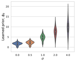
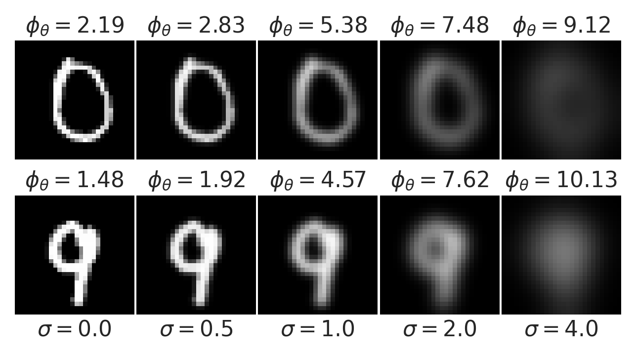
Figure 7: The prior $\phi_{\theta}$ learned by LPN on MNIST, evaluated at images blurred by Gaussian kernels with an increasing standard deviation $\sigma$. Left: the prior over 100 test images. Right: the prior at individual examples.

Besides perturbing the images by Gaussian noise and convex combination in Section 5.1, we also blur the images by Gaussian kernels with increasing standard deviations, with results shown in Figure 7. Again, the prior increases as the images become blurrier, coinciding with the distribution of real hand-written digit images.

References

- Adler et al. [2010] Amir Adler, Yacov Hel-Or, and Michael Elad. A shrinkage learning approach for single image super-resolution with overcomplete representations. In Computer Vision–ECCV 2010: 11th European Conference on Computer Vision, Heraklion, Crete, Greece, September 5-11, 2010, Proceedings, Part II 11, pages 622–635. Springer, 2010.
- Adler and Öktem [2018] Jonas Adler and Ozan Öktem. Learned primal-dual reconstruction. IEEE transactions on medical imaging, 37(6):1322–1332, 2018.
- Aggarwal et al. [2018] Hemant K Aggarwal, Merry P Mani, and Mathews Jacob. Modl: Model-based deep learning architecture for inverse problems. IEEE transactions on medical imaging, 38(2):394–405, 2018.
- Amos et al. [2017] Brandon Amos, Lei Xu, and J Zico Kolter. Input convex neural networks. In Proceedings of the 34th International Conference on Machine Learning, volume 70 of Proceedings of Machine Learning Research, pages 146–155. PMLR, 2017.
- Angelopoulos et al. [2022] Anastasios N Angelopoulos, Amit Pal Kohli, Stephen Bates, Michael Jordan, Jitendra Malik, Thayer Alshaabi, Srigokul Upadhyayula, and Yaniv Romano. Image-to-image regression with distribution-free uncertainty quantification and applications in imaging. In International Conference on Machine Learning, pages 717–730. PMLR, 2022.
- Arridge et al. [2019] Simon Arridge, Peter Maass, Ozan Öktem, and Carola-Bibiane Schönlieb. Solving inverse problems using data-driven models. Acta Numerica, 28:1–174, 2019.
- Attouch et al. [2010] Hédy Attouch, Jérôme Bolte, Patrick Redont, and Antoine Soubeyran. Proximal alternating minimization and projection methods for nonconvex problems: An approach based on the Kurdyka-ŁOjasiewicz inequality. Mathematics of Operations Research, 35(2):438–457, May 2010. ISSN 0364-765X. doi: 10.1287/moor.1100.0449.
- Attouch et al. [2013] Hedy Attouch, Jérôme Bolte, and Benar Fux Svaiter. Convergence of descent methods for semi-algebraic and tame problems: proximal algorithms, forward–backward splitting, and regularized Gauss–Seidel methods. Mathematical Programming. A Publication of the Mathematical Programming Society, 137(1):91–129, February 2013. ISSN 0025-5610, 1436-4646. doi: 10.1007/s10107-011-0484-9.
- Balke et al. [2022] Thilo Balke, Fernando Davis Rivera, Cristina Garcia-Cardona, Soumendu Majee, Michael Thompson McCann, Luke Pfister, and Brendt Egon Wohlberg. Scientific computational imaging code (scico). Journal of Open Source Software, 7(LA-UR-22-28555), 2022.
- Bauschke et al. [2012] Heinz H Bauschke, Sarah M Moffat, and Xianfu Wang. Firmly nonexpansive mappings and maximally monotone operators: Correspondence and duality. Set-Valued and Variational Analysis, 20(1):131–153, March 2012. ISSN 1877-0533, 1877-0541. doi: 10.1007/s11228-011-0187-7.
- Beck [2017] Amir Beck. First-order methods in optimization. SIAM, 2017.
- Beck and Teboulle [2009] Amir Beck and Marc Teboulle. A fast iterative shrinkage-thresholding algorithm for linear inverse problems. SIAM journal on imaging sciences, 2(1):183–202, 2009.
- Benning and Burger [2018] Martin Benning and Martin Burger. Modern regularization methods for inverse problems. Acta numerica, 27:1–111, 2018.
- Bertero et al. [2021] Mario Bertero, Patrizia Boccacci, and Christine De Mol. Introduction to inverse problems in imaging. CRC press, 2021.
- Boţ et al. [2016] Radu Ioan Boţ, Ernö Robert Csetnek, and Szilárd Csaba László. An inertial forward–backward algorithm for the minimization of the sum of two nonconvex functions. EURO Journal on Computational Optimization, 4(1):3–25, February 2016. ISSN 2192-4414. doi: 10.1007/s13675-015-0045-8.
- Boyd et al. [2011] Stephen Boyd, Neal Parikh, Eric Chu, Borja Peleato, Jonathan Eckstein, et al. Distributed optimization and statistical learning via the alternating direction method of multipliers. Foundations and Trends® in Machine learning, 3(1):1–122, 2011.
- Boyd and Vandenberghe [2004] Stephen P Boyd and Lieven Vandenberghe. Convex optimization. Cambridge university press, 2004.
- Bredies et al. [2010] Kristian Bredies, Karl Kunisch, and Thomas Pock. Total generalized variation. SIAM Journal on Imaging Sciences, 3(3):492–526, 2010.
- Bruckstein et al. [2009] Alfred M Bruckstein, David L Donoho, and Michael Elad. From sparse solutions of systems of equations to sparse modeling of signals and images. SIAM review, 51(1):34–81, 2009.
- Chambolle and Pock [2011] Antonin Chambolle and Thomas Pock. A first-order primal-dual algorithm for convex problems with applications to imaging. Journal of mathematical imaging and vision, 40:120–145, 2011.
- Chen et al. [2021] Dongdong Chen, Julián Tachella, and Mike E Davies. Equivariant imaging: Learning beyond the range space. In Proceedings of the IEEE/CVF International Conference on Computer Vision, pages 4379–4388, 2021.
- Chen et al. [2022a] Dongdong Chen, Julián Tachella, and Mike E Davies. Robust equivariant imaging: a fully unsupervised framework for learning to image from noisy and partial measurements. In Proceedings of the IEEE/CVF Conference on Computer Vision and Pattern Recognition, pages 5647–5656, 2022a.
- Chen et al. [2023] Dongdong Chen, Mike Davies, Matthias J Ehrhardt, Carola-Bibiane Schönlieb, Ferdia Sherry, and Julián Tachella. Imaging with equivariant deep learning: From unrolled network design to fully unsupervised learning. IEEE Signal Processing Magazine, 40(1):134–147, 2023.
- Chen et al. [2022b] Tianlong Chen, Xiaohan Chen, Wuyang Chen, Zhangyang Wang, Howard Heaton, Jialin Liu, and Wotao Yin. Learning to optimize: A primer and a benchmark. The Journal of Machine Learning Research, 23(1):8562–8620, 2022b.
- Chung et al. [2022] Hyungjin Chung, Jeongsol Kim, Michael T Mccann, Marc L Klasky, and Jong Chul Ye. Diffusion posterior sampling for general noisy inverse problems. arXiv preprint arXiv:2209.14687, 2022.
- Cohen et al. [2021a] Regev Cohen, Yochai Blau, Daniel Freedman, and Ehud Rivlin. It has potential: Gradient-driven denoisers for convergent solutions to inverse problems. Advances in Neural Information Processing Systems, 34:18152–18164, 2021a.
- Cohen et al. [2021b] Regev Cohen, Michael Elad, and Peyman Milanfar. Regularization by denoising via Fixed-Point projection (RED-PRO). SIAM journal on imaging sciences, 14(3):1374–1406, January 2021b. doi: 10.1137/20M1337168.
- Coste [2000] Michel Coste. An Introduction to Semialgebraic Geometry. Istituti editoriali e poligrafici internazionali, 2000. ISBN 9788881472253.
- Dabov et al. [2007] Kostadin Dabov, Alessandro Foi, Vladimir Katkovnik, and Karen Egiazarian. Image denoising by sparse 3-d transform-domain collaborative filtering. IEEE Transactions on image processing, 16(8):2080–2095, 2007.
- Darestani et al. [2021] Mohammad Zalbagi Darestani, Akshay S Chaudhari, and Reinhard Heckel. Measuring robustness in deep learning based compressive sensing. In International Conference on Machine Learning, pages 2433–2444. PMLR, 2021.
- Delbracio and Milanfar [2023] Mauricio Delbracio and Peyman Milanfar. Inversion by direct iteration: An alternative to denoising diffusion for image restoration. March 2023.
- Dold [2012] Albrecht Dold. Lectures on Algebraic Topology. Springer Science & Business Media, December 2012. ISBN 9783642678219.
- Elad and Aharon [2006] Michael Elad and Michal Aharon. Image denoising via sparse and redundant representations over learned dictionaries. IEEE Transactions on Image processing, 15(12):3736–3745, 2006.
- Engl et al. [1996] Heinz Werner Engl, Martin Hanke, and Andreas Neubauer. Regularization of inverse problems, volume 375. Springer Science & Business Media, 1996.
- Fang et al. [2023] Zhenghan Fang, Kuo-Wei Lai, Peter van Zijl, Xu Li, and Jeremias Sulam. Deepsti: Towards tensor reconstruction using fewer orientations in susceptibility tensor imaging. Medical image analysis, 87:102829, 2023.
- Feng et al. [2023] Berthy T Feng, Jamie Smith, Michael Rubinstein, Huiwen Chang, Katherine L Bouman, and William T Freeman. Score-based diffusion models as principled priors for inverse imaging. arXiv preprint arXiv:2304.11751, 2023.
- Frankel et al. [2015] Pierre Frankel, Guillaume Garrigos, and Juan Peypouquet. Splitting methods with variable metric for Kurdyka–Łojasiewicz functions and general convergence rates. Journal of optimization theory and applications, 165(3):874–900, 2015. ISSN 0022-3239. doi: 10.1007/s10957-014-0642-3.
- Gao et al. [2023] Angela F Gao, Oscar Leong, He Sun, and Katherine L Bouman. Image reconstruction without explicit priors. In ICASSP 2023-2023 IEEE International Conference on Acoustics, Speech and Signal Processing (ICASSP), pages 1–5. IEEE, 2023.
- Gilton et al. [2019] Davis Gilton, Greg Ongie, and Rebecca Willett. Neumann networks for linear inverse problems in imaging. IEEE Transactions on Computational Imaging, 6:328–343, 2019.
- Gilton et al. [2021] Davis Gilton, Gregory Ongie, and Rebecca Willett. Deep equilibrium architectures for inverse problems in imaging. IEEE Transactions on Computational Imaging, 7:1123–1133, 2021.
- Gregor and LeCun [2010] Karol Gregor and Yann LeCun. Learning fast approximations of sparse coding. In Proceedings of the 27th international conference on international conference on machine learning, pages 399–406, 2010.
- Gribonval [2011] Rémi Gribonval. Should penalized least squares regression be interpreted as maximum a posteriori estimation? IEEE transactions on signal processing: a publication of the IEEE Signal Processing Society, 59(5):2405–2410, May 2011. ISSN 1053-587X, 1941-0476. doi: 10.1109/TSP.2011.2107908.
- Gribonval and Nikolova [2020] Rémi Gribonval and Mila Nikolova. A characterization of proximity operators. Journal of Mathematical Imaging and Vision, 62(6-7):773–789, 2020.
- Hauptmann et al. [2023] Andreas Hauptmann, Subhadip Mukherjee, Carola-Bibiane Schönlieb, and Ferdia Sherry. Convergent regularization in inverse problems and linear plug-and-play denoisers. July 2023.
- Huang et al. [2021] Chin-Wei Huang, Ricky T Q Chen, Christos Tsirigotis, and Aaron Courville. Convex potential flows: Universal probability distributions with optimal transport and convex optimization. In International Conference on Learning Representations, 2021.
- Hurault et al. [2022a] Samuel Hurault, Arthur Leclaire, and Nicolas Papadakis. Gradient step denoiser for convergent plug-and-play. In International Conference on Learning Representations, 2022a.
- Hurault et al. [2022b] Samuel Hurault, Arthur Leclaire, and Nicolas Papadakis. Proximal denoiser for convergent plug-and-play optimization with nonconvex regularization. In International Conference on Machine Learning, pages 9483–9505. PMLR, 2022b.
- Jalal et al. [2021a] Ajil Jalal, Marius Arvinte, Giannis Daras, Eric Price, Alexandros G Dimakis, and Jon Tamir. Robust compressed sensing mri with deep generative priors. Advances in Neural Information Processing Systems, 34:14938–14954, 2021a.
- Jalal et al. [2021b] Ajil Jalal, Sushrut Karmalkar, Alexandros G Dimakis, and Eric Price. Instance-optimal compressed sensing via posterior sampling. arXiv preprint arXiv:2106.11438, 2021b.
- Kadkhodaie and Simoncelli [2021] Zahra Kadkhodaie and Eero Simoncelli. Stochastic solutions for linear inverse problems using the prior implicit in a denoiser. Adv. Neural Inf. Process. Syst., 34:13242–13254, 2021.
- Kamilov et al. [2023] Ulugbek S Kamilov, Charles A Bouman, Gregery T Buzzard, and Brendt Wohlberg. Plug-and-play methods for integrating physical and learned models in computational imaging: Theory, algorithms, and applications. IEEE Signal Processing Magazine, 40(1):85–97, 2023.
- Kawar et al. [2021] Bahjat Kawar, Gregory Vaksman, and Michael Elad. SNIPS: Solving noisy inverse problems stochastically. May 2021.
- Kawar et al. [2022] Bahjat Kawar, Michael Elad, Stefano Ermon, and Jiaming Song. Denoising diffusion restoration models. January 2022.
- Kingma and Ba [2014] Diederik P Kingma and Jimmy Ba. Adam: A method for stochastic optimization. arXiv preprint arXiv:1412.6980, 2014.
- Kobler et al. [2017] Erich Kobler, Teresa Klatzer, Kerstin Hammernik, and Thomas Pock. Variational networks: Connecting variational methods and deep learning. In Pattern Recognition, Lecture Notes in Computer Science, pages 281–293. Springer, Cham, September 2017. ISBN 9783319667089, 9783319667096. doi: 10.1007/978-3-319-66709-6“˙23.
- Lai et al. [2020] Kuo-Wei Lai, Manisha Aggarwal, Peter van Zijl, Xu Li, and Jeremias Sulam. Learned proximal networks for quantitative susceptibility mapping. In Medical Image Computing and Computer Assisted Intervention–MICCAI 2020: 23rd International Conference, Lima, Peru, October 4–8, 2020, Proceedings, Part II 23, pages 125–135. Springer, 2020.
- LeCun [1998] Yann LeCun. The mnist database of handwritten digits. http://yann. lecun. com/exdb/mnist/, 1998.
- Liu et al. [2019] Jialin Liu, Xiaohan Chen, Zhangyang Wang, and Wotao Yin. ALISTA: Analytic weights are as good as learned weights in LISTA. In International Conference on Learning Representations, 2019.
- Liu et al. [2022] Jiaming Liu, Xiaojian Xu, Weijie Gan, Ulugbek Kamilov, et al. Online deep equilibrium learning for regularization by denoising. Advances in Neural Information Processing Systems, 35:25363–25376, 2022.
- Liu et al. [2018] Ziwei Liu, Ping Luo, Xiaogang Wang, and Xiaoou Tang. Large-scale celebfaces attributes (celeba) dataset. Retrieved August, 15(2018):11, 2018.
- Lojasiewicz [1963] Stanislaw Lojasiewicz. Une propriété topologique des sous-ensembles analytiques réels. Les équations aux dérivées partielles, 117:87–89, 1963.
- Lunz et al. [2018] Sebastian Lunz, Ozan Öktem, and Carola-Bibiane Schönlieb. Adversarial regularizers in inverse problems. Advances in neural information processing systems, 31, 2018.
- Mallat [1999] Stéphane Mallat. A wavelet tour of signal processing. Elsevier, 1999.
- Mardani et al. [2018] Morteza Mardani, Qingyun Sun, David Donoho, Vardan Papyan, Hatef Monajemi, Shreyas Vasanawala, and John Pauly. Neural proximal gradient descent for compressive imaging. Advances in Neural Information Processing Systems, 31, 2018.
- McCann et al. [2017] Michael T McCann, Kyong Hwan Jin, and Michael Unser. Convolutional neural networks for inverse problems in imaging: A review. IEEE Signal Processing Magazine, 34(6):85–95, 2017.
- McCollough [2016] C McCollough. Tu-fg-207a-04: overview of the low dose ct grand challenge. Medical physics, 43(6Part35):3759–3760, 2016.
- Monga et al. [2021] Vishal Monga, Yuelong Li, and Yonina C Eldar. Algorithm unrolling: Interpretable, efficient deep learning for signal and image processing. IEEE Signal Processing Magazine, 38(2):18–44, March 2021. ISSN 1558-0792. doi: 10.1109/MSP.2020.3016905.
- Moreau [1965] Jean-Jacques Moreau. Proximité et dualité dans un espace hilbertien. Bulletin de la Société mathématique de France, 93:273–299, 1965.
- Mukherjee et al. [2020] Subhadip Mukherjee, Sören Dittmer, Zakhar Shumaylov, Sebastian Lunz, Ozan Öktem, and Carola-Bibiane Schönlieb. Learned convex regularizers for inverse problems. arXiv preprint arXiv:2008.02839, 2020.
- Mukherjee et al. [2021] Subhadip Mukherjee, Marcello Carioni, Ozan Öktem, and Carola-Bibiane Schönlieb. End-to-end reconstruction meets data-driven regularization for inverse problems. Advances in Neural Information Processing Systems, 34:21413–21425, 2021.
- Ongie et al. [2020] Gregory Ongie, Ajil Jalal, Christopher A Metzler, Richard G Baraniuk, Alexandros G Dimakis, and Rebecca Willett. Deep learning techniques for inverse problems in imaging. IEEE Journal on Selected Areas in Information Theory, 1(1):39–56, 2020.
- Parikh and Boyd [2014] Neal Parikh and Stephen Boyd. Proximal algorithms. Foundations and Trends® in Optimization, 1(3):127–239, 2014. ISSN 2167-3888. doi: 10.1561/2400000003.
- Richter-Powell et al. [2021] Jack Richter-Powell, Jonathan Lorraine, and Brandon Amos. Input convex gradient networks. arXiv preprint arXiv:2111.12187, 2021.
- Rockafellar and Wets [1998] R Tyrell Rockafellar and Roger J-B Wets. Variational Analysis. Grundlehren der mathematischen Wissenschaften. Springer-Verlag Berlin Heidelberg, 1 edition, 1998. ISBN 9783642024313, 9783540627722. doi: 10.1007/978-3-642-02431-3.
- Romano and Elad [2015] Yaniv Romano and Michael Elad. Boosting of image denoising algorithms. SIAM Journal on Imaging Sciences, 8(2):1187–1219, 2015.
- Romano et al. [2017] Yaniv Romano, Michael Elad, and Peyman Milanfar. The little engine that could: Regularization by denoising (red). SIAM Journal on Imaging Sciences, 10(4):1804–1844, 2017.
- Rudin et al. [1992] Leonid I Rudin, Stanley Osher, and Emad Fatemi. Nonlinear total variation based noise removal algorithms. Physica D: nonlinear phenomena, 60(1-4):259–268, 1992.
- Rudin [1976] Walter Rudin. Principles of mathematical analysis. McGraw-Hill, New York, 3 edition, 1976. ISBN 9780070542358.
- Ryu et al. [2019] Ernest Ryu, Jialin Liu, Sicheng Wang, Xiaohan Chen, Zhangyang Wang, and Wotao Yin. Plug-and-Play methods provably converge with properly trained denoisers. In Kamalika Chaudhuri and Ruslan Salakhutdinov, editors, Proceedings of the 36th International Conference on Machine Learning, volume 97 of Proceedings of Machine Learning Research, pages 5546–5557. PMLR, 2019.
- Shenoy et al. [2023] Vineet R Shenoy, Tim K Marks, Hassan Mansour, and Suhas Lohit. Unrolled ippg: Video heart rate estimation via unrolling proximal gradient descent. In 2023 IEEE International Conference on Image Processing (ICIP), pages 2715–2719. IEEE, 2023.
- Sreehari et al. [2016] Suhas Sreehari, S V Venkatakrishnan, Brendt Wohlberg, Gregery T Buzzard, Lawrence F Drummy, Jeffrey P Simmons, and Charles A Bouman. Plug-and-Play priors for bright field electron tomography and sparse interpolation. IEEE Transactions on Computational Imaging, 2(4):408–423, December 2016. ISSN 2333-9403. doi: 10.1109/TCI.2016.2599778.
- Stein and Shakarchi [2005] Elias M Stein and Rami Shakarchi. Real Analysis: Measure Theory, Integration, and Hilbert Spaces. Princeton University Press, April 2005. ISBN 9780691113869.
- Sulam et al. [2014] Jeremias Sulam, Boaz Ophir, and Michael Elad. Image denoising through multi-scale learnt dictionaries. In 2014 IEEE International Conference on Image Processing (ICIP), pages 808–812. IEEE, 2014.
- Sulam et al. [2019] Jeremias Sulam, Aviad Aberdam, Amir Beck, and Michael Elad. On multi-layer basis pursuit, efficient algorithms and convolutional neural networks. IEEE transactions on pattern analysis and machine intelligence, 42(8):1968–1980, 2019.
- Sulam et al. [2020] Jeremias Sulam, Ramchandran Muthukumar, and Raman Arora. Adversarial robustness of supervised sparse coding. Advances in neural information processing systems, 33:2110–2121, 2020.
- Sun and Bouman [2021] He Sun and Katherine L Bouman. Deep probabilistic imaging: Uncertainty quantification and multi-modal solution characterization for computational imaging. In Proceedings of the AAAI Conference on Artificial Intelligence, volume 35, pages 2628–2637, 2021.
- Sun et al. [2019] Yu Sun, Brendt Wohlberg, and Ulugbek S Kamilov. An online Plug-and-Play algorithm for regularized image reconstruction. IEEE Transactions on Computational Imaging, 5(3):395–408, September 2019. ISSN 2333-9403. doi: 10.1109/TCI.2019.2893568.
- Sun et al. [2021] Yu Sun, Zihui Wu, Xiaojian Xu, Brendt Wohlberg, and Ulugbek S Kamilov. Scalable Plug-and-Play ADMM with convergence guarantees. IEEE Transactions on Computational Imaging, 7:849–863, 2021. ISSN 2333-9403. doi: 10.1109/TCI.2021.3094062.
- Tachella et al. [2019] Julián Tachella, Yoann Altmann, Nicolas Mellado, Aongus McCarthy, Rachael Tobin, Gerald S Buller, Jean-Yves Tourneret, and Stephen McLaughlin. Real-time 3d reconstruction from single-photon lidar data using plug-and-play point cloud denoisers. Nature communications, 10(1):4984, 2019.
- Tachella et al. [2022] Julián Tachella, Dongdong Chen, and Mike Davies. Unsupervised learning from incomplete measurements for inverse problems. Advances in Neural Information Processing Systems, 35:4983–4995, 2022.
- Tachella et al. [2023] Julián Tachella, Dongdong Chen, and Mike Davies. Sensing theorems for unsupervised learning in linear inverse problems. Journal of Machine Learning Research, 24(39):1–45, 2023.
- Tan et al. [2023] Hong Ye Tan, Subhadip Mukherjee, Junqi Tang, and Carola-Bibiane Schönlieb. Provably convergent Plug-and-Play Quasi-Newton methods. March 2023.
- Teneggi et al. [2023] Jacopo Teneggi, Matthew Tivnan, Web Stayman, and Jeremias Sulam. How to trust your diffusion model: A convex optimization approach to conformal risk control. In International Conference on Machine Learning, pages 33940–33960. PMLR, 2023.
- Teodoro et al. [2018] Afonso M Teodoro, Jose M Bioucas-Dias, and Mario A T Figueiredo. A convergent image fusion algorithm using Scene-Adapted Gaussian-Mixture-Based denoising. IEEE transactions on image processing: a publication of the IEEE Signal Processing Society, September 2018. ISSN 1057-7149, 1941-0042. doi: 10.1109/TIP.2018.2869727.
- Themelis and Patrinos [2020] Andreas Themelis and Panagiotis Patrinos. Douglas–Rachford splitting and ADMM for nonconvex optimization: Tight convergence results. SIAM journal on optimization: a publication of the Society for Industrial and Applied Mathematics, 30(1):149–181, January 2020. ISSN 1052-6234. doi: 10.1137/18M1163993.
- Tian et al. [2020] Chunwei Tian, Lunke Fei, Wenxian Zheng, Yong Xu, Wangmeng Zuo, and Chia-Wen Lin. Deep learning on image denoising: An overview. Neural Networks, 131:251–275, 2020.
- Tikhonov and Arsenin [1977] Andrey N Tikhonov and Vasiliy Y Arsenin. Solutions of ill-posed problems. vh winston & sons, 1977.
- Tolooshams et al. [2023] Bahareh Tolooshams, Satish Mulleti, Demba Ba, and Yonina C Eldar. Unrolled compressed blind-deconvolution. IEEE Transactions on Signal Processing, 2023.
- Venkatakrishnan et al. [2013] Singanallur V Venkatakrishnan, Charles A Bouman, and Brendt Wohlberg. Plug-and-play priors for model based reconstruction. In 2013 IEEE Global Conference on Signal and Information Processing, pages 945–948. IEEE, 2013.
- Willemink and Noël [2019] Martin J Willemink and Peter B Noël. The evolution of image reconstruction for ct—from filtered back projection to artificial intelligence. European radiology, 29:2185–2195, 2019.
- Xu et al. [2020] Xiaojian Xu, Yu Sun, Jiaming Liu, Brendt Wohlberg, and Ulugbek S Kamilov. Provable convergence of Plug-and-Play priors with MMSE denoisers. IEEE Signal Processing Letters, 27:1280–1284, 2020. ISSN 1558-2361. doi: 10.1109/LSP.2020.3006390.
- Yu et al. [2019] Songhyun Yu, Bumjun Park, and Jechang Jeong. Deep iterative down-up cnn for image denoising. In Proceedings of the IEEE/CVF conference on computer vision and pattern recognition workshops, pages 0–0, 2019.
- Zhang et al. [2017a] Kai Zhang, Wangmeng Zuo, Yunjin Chen, Deyu Meng, and Lei Zhang. Beyond a gaussian denoiser: Residual learning of deep cnn for image denoising. IEEE transactions on image processing, 26(7):3142–3155, 2017a.
- Zhang et al. [2017b] Kai Zhang, Wangmeng Zuo, Shuhang Gu, and Lei Zhang. Learning deep cnn denoiser prior for image restoration. In Proceedings of the IEEE conference on computer vision and pattern recognition, pages 3929–3938, 2017b.
- Zhang et al. [2020] Kai Zhang, Luc Van Gool, and Radu Timofte. Deep unfolding network for image super-resolution. In Proceedings of the IEEE/CVF conference on computer vision and pattern recognition, pages 3217–3226, 2020.
- Zhang et al. [2021] Kai Zhang, Yawei Li, Wangmeng Zuo, Lei Zhang, Luc Van Gool, and Radu Timofte. Plug-and-play image restoration with deep denoiser prior. IEEE Transactions on Pattern Analysis and Machine Intelligence, 44(10):6360–6376, 2021.
- Zhang et al. [2018] Richard Zhang, Phillip Isola, Alexei A Efros, Eli Shechtman, and Oliver Wang. The unreasonable effectiveness of deep features as a perceptual metric. In Proceedings of the IEEE conference on computer vision and pattern recognition, pages 586–595, 2018.
- Zhu et al. [2018] Bo Zhu, Jeremiah Z Liu, Stephen F Cauley, Bruce R Rosen, and Matthew S Rosen. Image reconstruction by domain-transform manifold learning. Nature, 555(7697):487–492, 2018.
- Zou et al. [2023] Zihao Zou, Jiaming Liu, Brendt Wohlberg, and Ulugbek S Kamilov. Deep equilibrium learning of explicit regularizers for imaging inverse problems. arXiv preprint arXiv:2303.05386, 2023.