Pyramidal Hidden Markov Model For Multivariate Time Series Forecasting

Abstract

The Hidden Markov Model (HMM) can predict the future value of a time series based on its current and previous values, making it a powerful algorithm for handling various types of time series. Numerous studies have explored the improvement of HMM using advanced techniques, leading to the development of several variations of HMM. Despite these studies indicating the increased competitiveness of HMM compared to other advanced algorithms, few have recognized the significance and impact of incorporating multistep stochastic states into its performance. In this work, we propose a Pyramidal Hidden Markov Model (PHMM) that can capture multiple multistep stochastic states. Initially, a multistep HMM is designed for extracting short multistep stochastic states. Next, a novel time series forecasting structure is proposed based on PHMM, which utilizes pyramid-like stacking to adaptively identify long multistep stochastic states. By employing these two schemes, our model can effectively handle non-stationary and noisy data, while also establishing long-term dependencies for more accurate and comprehensive forecasting. The experimental results on diverse multivariate time series datasets convincingly demonstrate the superior performance of our proposed PHMM compared to its competitive peers in time series forecasting.

Index Terms—  Time Series Forecasting, Multistep Stochastic States, Multistep Hidden Markov Model

1 Introduction

Time series forecasting is crucial in various social domains, facilitating resource management and decision-making. For instance, in medical diagnosis, past data can assist in the timely detection and control of potential diseases. Nevertheless, early forecasting presents some challenges, including: i) violating stability assumptions of traditional models hinders accurate prediction of future trends, leading to non-stationarity of data; and ii) undergoing distributional shifts across various working conditions results in Out-Of-Distribution (OOD) forecasting, which poses a challenge for many existing supervised learning models.

For this reason, numerous studies utilize Hidden Markov Models (HMM) to address nonstationary data and OOD forecasting as they can work with stochastic states rather than fitting a specific distribution. However, most of HMMs, only accounting for single-step stochastic state transitions, encounters long-term forecasting challenges when applied to real-world time series that can be described as predominantly consisting of multiple multistep stochastic state. Consequently, such a model will be hard to achieve forecasting well, especially in terms of long-term prediction. Thus, in this work, to enhance the identification of multistep stochastic states, we introduce a novel Hidden Markov Model with multiple steps. Our model incorporates an attention mechanism into the data input of a multistep time window, enabling realistic capture of these states in a time series. Moreover, we employ a stacking technique to appropriately increase the depth of the model structure, enhancing its adaptability to stochastic states with varying step sizes and improving its predictive capability through deep stacking.

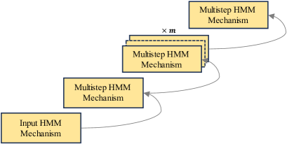
Fig. 1: Brief structure of our model.

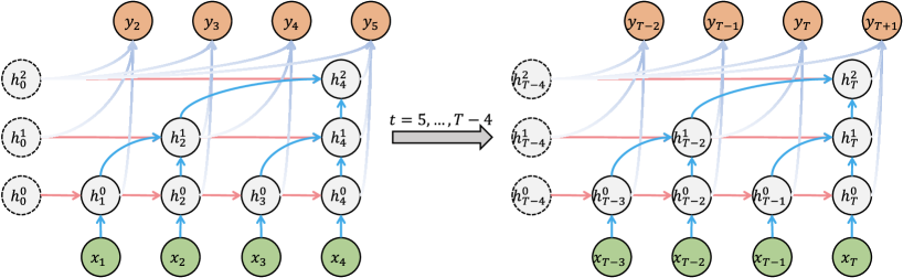
Fig. 2: Pyramidal Hidden Markov Model with Directed Acyclic Graphs.

We utilize a training method based on deep generative models, which learn from a low-dimensional potential space assumed to reside on known Riemannian manifolds. Moreover, the neutralized HMM is optimized using the Maximum Likelihood Estimation (MLE) method, as opposed to the traditional Expectation-Maximization (EM) method. Experimental results provide convincing evidence that the proposed PHMM outperforms its competitors for time series forecasting and effectively addresses the limitations of the conventional HMM in capturing the multistep stochastic state.

Table 1: Others VS. Our model.

Method	DTW	WEASEL+ MUSE (2018)	MLSTM -FCN (2019)	TapNet (2020)	ShapeNet (2019)	Rocket (2020)	Wins
WEASEL+MUSE	✓		✓				13
MLSTM-FCN	✓	✓					14
TapNet	✓	✓	✓				14
ShapeNet	✓	✓	✓	✓			14
ROCKET	✓			✓			9
Our Model	✓	✓	✓	✓	✓	✓	15

2 Related Work

Traditional time series forecasting methods typically require continuous, complete time series data, which refers to labeled values or supervisory signals at each time step for future phases. However, our time series forecasting scenario can tolerate missing data or outliers. In real-world scenarios, outliers are often observed due to noise in sensor sampling or errors in data transmission.

Other approaches similar to ours are modeling time series data [licausal and related citations in his article]. Most of these works use Multilayer Perception (MLP) or Convolutional Neural Networks (CNN) for feature extraction; and neural networked HMMs are used to generate trajectories for extracting features. Deep generative networks are used to learn from low-dimensional Riemannian spaces, a technique that trains the encoder. However, many of these studies fail to acknowledge the significance of the multistep feature in the hidden random state for creating long-term dependencies. In contrast, our model captures the multistep random states to establish long-term dependencies, addressing the neglect of this issue in previous research.

In the experimental session, we present the classification accuracy, average ranking, and wins/losses for each dataset on the test dataset. We compute the Mean Per Class Error (MPCE) as the average error per class across all datasets. Furthermore, we calculate the mean error per class for all datasets by applying the described procedure, as depicted in equation (1).

$$\eta=\frac{1}{n}\sum_{i=1}^{n}|v_{i}|=\frac{1}{n}\sum_{i=1}^{n}|x_{i}-\bar{x}|.$$ (1)

We also performed the Friedman test and the Wilcoxon signed rank test using Holm’s $\alpha$ (5%) following the procedure described therein. The Friedman test is a non-parametric statistical test used to demonstrate the significance of differences in performance across all methods.The Wilcoxon signed rank test is a non-parametric statistical test based on the assumption that the median of the ranks is the same between our methods and any baseline.

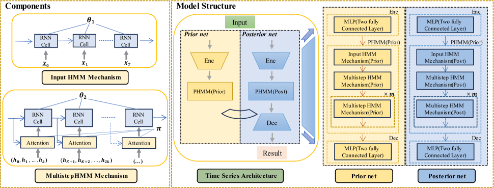
Fig. 3: Structure Drawing

3 Preliminaries

Directed Acyclic Graph (DAG). The DAG is denoted as $G\in(V,E)$ with $V$, $E$ respectively denoting the node and edge set. Each arrow $x\to y$ in $E$ represents a direct effect of $x$ on $y$. The structural equations define the generating mechanisms for each each node in $V$. Specifically, for $V\in\{v_{1},...,v_{k}\}$ ,the mechanisms associated with the structural equations(defined as ${f_{i}}_{v_{i}\in V}$) are defined as:$\{v_{i}\leftarrow f_{i}(Pa(V_{i}),{\epsilon}_{i})\}_{v_{i}\in V}$.

To further visualise our model, our DAG is given as shown in Fig. 2. We introduce $m$ hidden variables ${h_{t}^{0},h_{t}^{1},\ldots,h_{t}^{m}}$ which are passed in $m$ hidden Markov chains, the meaning of which is denoted as hidden variables of $k^{m}$ steps. Each hidden variable $h_{t}^{m}$ ($m=0,1,\ldots,m$) is generated from the outputs ${o_{t-k+1}^{m-1},o_{t-k+2}^{m-1},\ldots,o_{t}^{m-1}}$ and $h_{t-1}^{m}$ of the previous section. Finally, the hidden variables from each chain are concatenated and used as output for performing the prediction task at each time step. Subsequently, we provide a detailed explanation of the model definition and the learning methodology in the subsequent sections.

4 Model

Problem Statement. A multivariate time series can be represented as $X=\{X_{1},X_{2},\ldots,X_{n}\}$, where $n$ denotes the number of samples. Each sample $X_{i}$ consists of a series of events, $X_{i}=\{x_{i_{1}},x_{i\ 2},\ldots,x_{i\ m}\}$, where each $x_{ij}$ denotes the value of the observed sequence at each time step $t$, and each time step can encompass a different number of record dimensions. In particular, $x_{ij}\in\mathbb{R}^{D}$.

Our goal is to train a prediction model that can perform both the classification task $f:X_{i}\rightarrow y_{i}$ and the prediction task $f:x_{i\ m}\rightarrow x_{i\ m+1},\ x_{i\ m+2},\ldots,\ x_{i\ m+p}$, where $p$ denotes the number of prediction steps.

4.1 Pyramidal Hidden Markov Model

To describe the model design, we introduce the directed acyclic graph of DAG as shown in Figure 2. As a new Hidden Markov Model design, our model is named Pyramidal Hidden Markov Model. Our model is defined in detail as follows:

Definition 4.1 (Pyramidal Hidden Markov Model) Pyramidal Hidden Markov Model of directed acyclic graph DAG is formed. where the model is defined as $F$, $F\triangleq F_{t}$, where $F_{t}\triangleq x_{t}\leftarrow f(x_{t},h_{0}^{t},\epsilon_{h0}^{t},h_{1}^{t},\epsilon_{h1}^{t},h_{2}^{t},\ldots,h_{m}^{t})$ for $t<T$. $F_{T}$ additionally contains $y_{t}\leftarrow f(y,h_{t0},h_{t},\ldots,h_{t})$. where ${\epsilon_{x_{t}},\epsilon_{h0_{t}},\epsilon_{h1_{t}},\ldots,\epsilon_{h_{m-1_{t}}}}$ are independently exogenous variables, $\epsilon_{x_{t}}$ for $t<T$ similarly $\epsilon_{h0_{t}}$, $\epsilon_{h1_{t}}$, $\ldots$, and $\epsilon_{h_{m-1_{t}}}$are identically distributed at time $t$.

Input Hidden Markov Mechanism

The input Hidden Markov Model (HMM) is implemented using a neuralized HMM, represented in the figure as an GRU with shared parameters $\theta$. At each time step, an output result $o_{t}$ is generated and retained for output and input in multistep HMM mechanisms. The detailed definitions of prior and posterior are provided below.

Based on the Markov condition, the joint distribution corresponding to the Hidden Markov Chain is:

$$\begin{aligned} p(h_{t<T}|x_{t<T},y_{T})&=p(y_{T}|h_{T})*\prod_{t=1}^{T-1}\Big{(}p(h_{t}|h_{t-1},x_{t-1})\\ p(x_{t}|h_{t})\Big{)},\end{aligned}$$ (2)

$\text{here}\left\{p\left(h_{t}\middle|h_{t-1},x_{t-1}\right)\right\}_{t},q_{\phi}\left(h_{t<T}\middle|x_{t<T},y_{T}\right).\left\{p(x_{t}\middle|h_{t})\right\}_{t}$ denote the a priori, a posteriori, and a generative model respectively.

Priori. For a priori $P_{\psi}\left(h_{t}\middle|h_{t-1},x_{t-1}\right)$, it can be written as:

$$p_{\psi}\left(h_{t}\middle|h_{t-1},x_{t-1}\right)=\prod_{o}{p_{\psi}\left(o_{t}\middle|o_{t-1},x_{t-1}\right)},$$ (3)

where $o\in\left\{h\right\}$, $p_{\psi}\left(h_{t}\middle|h_{t-1},x_{t-1}\right)$ are the distributions at each time $t$ as $N(\mu_{\psi}\left(h_{t-1},x_{t-1}\right),\sum_{\psi}(h_{t-1},x_{t-1}))$).

The $\Big{\{}\mu_{\psi}\left(h_{t-1},x_{t-1}\right)\Big{\}}_{t}$ and $\left\{\sum_{\psi}(h_{t-1},x_{t-1})\right\}_{t}$ are parametrized by a network of Gated Recurrent Unit (GRU). This GRU is designed to capture single-step dependencies, which have been employed in; following the GRU are two fully connected layers, one outputting an average vector and one outputting a logarithmic vector of hidden variables.

Posterior. For the posterior $q_{\phi}$ is an imitation of $p_{\psi}($also $p)$. It also uses the heavily parameterised $p_{\psi}=p_{\psi}(h_{t<T}|u_{t<T},y_{T}).$ In the case of a reparameterisation using $p_{\psi}$ and a mean field decomposition, the posterior is given by the following equation:

$$\begin{aligned} q_{\phi}\left(h_{t<T}\middle|x_{t<T},y_{T}\right)=&\frac{q_{\phi}\left(y_{T}|h_{T-1}\right)}{q_{\phi}\left(y_{T}|x_{t<T}\right)}{\ast}\\ &\prod_{t<T}{q_{\phi}(h_{t}|x_{t},h_{t-1})},\end{aligned}$$ (4)

here $q_{\phi}\left(h_{t}\middle|x_{t},h_{t-1}\right)\sim N\left(\mu\left(x_{t},h_{t-1}\right),\sum\left(x_{t},h_{t-1}\right)\right)$.

In particular, the posterior network $q_{\phi}\left(h_{t}\middle|h_{t-1},x_{t}\right)$ is an encoding of the time series input $x$ by a two-layer fully-connected layer.

Multistep Hidden Markov Mechanism

The Multistep Hidden Markov Models(MHMM) utilizes a neuralized Hidden Markov Model with an attention mechanism, consisting of a GRU with shared parameter $\theta$ and an attention mechanism with shared parameter $\pi$. The input in the time window $\{x_{k+1},x_{k+2},\ldots,x_{2k}\}$ (with step size $k$) is multiplied by the weights resulting from the attention mechanism.

Based on the Markov condition, the corresponding joint distribution of the Hidden Markov chain is:

$$\begin{aligned} p(h_{1:k:T}|o_{1:k:T},y_{T})=&p(y_{T+1}|h_{T}){\ast}\prod_{t<\left[\frac{T}{k}\right]}p(h_{kt}|h_{kt-k},\\ &x_{kt-k+1},\ldots,x_{kt})p(x_{kt}|h_{kt}),\end{aligned}$$ (5)

here $\{p(h_{kt}|h_{kt-k},x_{kt-k+1},\ldots,x_{kt})\}_{t},q_{\phi}(h_{t<T}|x_{t<T},\\ y_{T}),p(x_{kt}|h_{kt})$ denote the a priori model, the posterior model and the generative model, respectively.

Priori. For the prior $\mathbf{P}_{\psi}(h_{kt}|h_{kt-1},x_{kt-k+1},\ldots,x_{kt})$, it can be written as:

$$\begin{aligned} \mathbf{P}_{\psi}(h_{kt}|h_{kt-1},x_{kt-k+1},\ldots,x_{kt})=\prod_{o}p_{\psi}(o_{t}|o_{t-1},\\ x_{kt-k+1},\ldots,x_{kt}),\end{aligned}$$ (6)

$\text{where }o\in\{h\}$, $P_{\psi}(h_{kt}|h_{kt-k},x_{kt-k+1},\ldots,x_{kt})$ is the distribution at each time$t\text{ as }N(\mu_{\psi}(h_{kt-k},x_{kt-k+1},\ldots,x_{kt}),\\ \Sigma_{\psi}(h_{kt-k},x_{kt-k+1},\ldots,x_{kt}))$.

$\text{The }\{\mu_{\psi}(h_{kt-k},x_{kt-k+1},\ldots,x_{kt})\}_{t}(\text{and}\{\Sigma_{\psi}(h_{kt-k},\\ x_{kt-k+1},\ldots,x_{kt})\}_{t})$are parametrized by the network of gated recurrent unit (GRU). And the different inputs are weighted at input using attention, which is designed to capture multistep dependencies; after the GRU are two fully connected layers, one outputting the mean vector and one outputting the logarithmic vector of hidden variables.

Posterior. For the posterior $q_{\phi}$ is an closingly mimic for $p_{\psi}$(also $p$). It also uses the heavily parameterised $p_{\psi}=p_{\psi}(h_{t<T}|u_{t<T},y_{T})$. In the case of the reparameterisation using $p_{\psi}$ and the mean field decomposition, the posterior is given by the following equation:

$$\begin{aligned} q_{\phi}(h_{1:k:T}|x_{1:k:T},y_{T})=\frac{q_{\phi}(y_{T}|h_{T-1})}{q_{\phi}(y_{T}|o_{1:k:T})}\ast\prod_{t<\left[\frac{T}{k}\right]}q_{\phi}(h_{kt}|\\ h_{kt-k},x_{kt-k+1},x_{kt-k+2},\ldots,x_{kt}),\end{aligned}$$ (7)

$\text{where }q_{\phi}(h_{kt}|h_{kt-k},x_{kt-k+1},\ldots,x_{kt})\sim N(\mu(h_{kt-k},\\ x_{kt-k+1},\ldots,x_{kt}),\sigma(h_{kt-k},x_{kt-k+1},\ldots,x_{kt}))$.

Similarly, the posterior network represented by symbol $q_{\phi}(h_{kt}|h_{kt-k},x_{kt-k+1},\ldots,x_{kt})$ is encoded by a learnable weight matrix of size$1\times k$, weighting the inputs of multiple time steps, and feeding it into a two-layer fully connected network.

Table 2: Classification results

Dataset	EDI	DTWI	DTWO	WEASEL +MUSE (2018)	MLSTM -FCN (2019)	MrEQL (2019)	TapNet (2020)	ShapeNet (2021)	ROCKET (2020)	MiniRocket (2021)	RLPAM (2022)	UCS	PHMM (ours)
AWR	0.970	0.980	0.987	0.990	0.510	0.993	0.59	0.61	0.993	0.992	0.923	0.570	0.970
AF	0.267	0.267	0.200	0.333	0.260	0.267	0.33	0.40	0.067	0.133	0.733	0.467	0.733
BM	0.675	1.000	0.975	1.000	0.660	0.950	0.75	0.75	1.000	1.000	1.000	0.737	1.000
CT	0.964	0.969	0.990	0.990	0.890	0.970	0.89	0.90	N/A	0.993	0.978	0.816	0.988
CR	0.944	0.986	1.000	1.000	0.917	0.986	0.958	0.986	1.000	0.986	0.764	1.000	0.972
EP	0.667	0.978	0.964	1.000	0.761	0.993	0.971	0.987	0.993	1.000	0.826	0.978	0.980
EC	0.293	0.304	0.323	0.430	0.373	0.555	0.323	0.312	0.380	0.468	0.369	0.354	0.451
FD	0.519	0.513	0.529	0.545	0.545	0.545	0.556	0.602	0.630	0.620	0.621	0.520	0.626
FM	0.550	0.520	0.530	0.490	0.580	0.550	0.530	0.580	0.530	0.550	0.640	0.610	0.620
HMD	0.279	0.306	0.231	0.365	0.365	0.149	0.378	0.338	0.446	0.392	0.635	0.432	0.514
HB	0.620	0.659	0.717	0.727	0.663	0.741	0.751	0.756	0.726	0.771	0.779	0.737	0.741
IW	0.128	N/A	0.115	N/A	0.167	N/A	0.208	0.250	N/A	0.595	0.352	0.125	0.657
JV	0.924	0.959	0.949	0.973	0.976	0.922	0.965	0.984	0.965	0.989	0.935	0.743	0.981
LIB	0.833	0.894	0.872	0.878	0.856	0.872	0.850	0.856	0.906	0.922	0.794	0.550	0.877
LSST	0.456	0.575	0.551	0.59	0.373	0.588	0.568	0.590	0.639	0.643	0.644	0.350	0.722
MI	0.510	0.390	0.500	0.500	0.510	0.520	0.590	0.610	0.560	0.55	0.610	0.570	0.580
RS	0.868	0.842	0.803	0.934	0.803	0.868	0.868	0.882	0.921	0.868	0.868	0.743	0.840
SRS1	0.771	0.765	0.775	0.710	0.874	0.679	0.652	0.782	0.846	0.925	0.802	0.577	0.912
SRS2	0.483	0.533	0.539	0.460	0.472	0.572	0.550	0.530	0.578	0.540	0.632	0.622	0.567
UWGL	0.881	0.869	0.903	0.936	0.891	0.872	0.894	0.906	0.938	0.938	0.944	0.416	0.914
Avg. Rank
MPCE
Win\Ties
Our 1-to-1-Wins
Our 1-to-1-Losses
Wilcoxon Test p-value

- Accuracy results are sorted by deviations between PHMM and the best performing baselines. The classifcation accuracy of the baselines on the UEA archive datasets are obtained from their original papers, except ROCKET which is run using the code open-sourced.

4.2 Learning Method

To learn our proposed pyramidal Hidden Markov Model, we first introduce a sequential VAE structure, based on the VAE architecture and acting on the section shown in Figure. This ELBO is accompanied by a simplified $q_{\emptyset}(H_{1:T}|x_{1:T-1},y_{T})$$(H=\{h^{0},h^{1},\ldots,h^{m}\})$ variable distribution such as $\mathbb{E}_{p(x_{t<T},y_{T})}\left[L_{q_{\emptyset},p_{\psi}}\right]$.

Generated Part. For each time $t$, the generative model is a p.d.f. of a Gaussian distribution parameterised by a two-layer fully connected network to reconstruct the input sequence $x$. The $q_{\phi}(y_{T}|H_{T-1})$ is either a fully connected layer classifier with softmax as activation function or a fully connected layer predictor with no activation function.

Reformulation. Substituting the posterior $p_{\psi}$ and the prior $q_{\emptyset}$ in the above equation, we reformulate the ELBO as

$$\mathbb{E}_{p(x_{t<T},y_{T})}\left[\log q_{\emptyset}\left(y_{T}\middle|x_{<T}\right)+\sum_{t<T}\mathcal{L}_{q_{\emptyset},p_{\psi}}^{t}\right],$$ (8)

$$\mathcal{L}_{q_{\emptyset},p_{\psi}}^{t}=\mathbb{E}_{p\left(H_{t}\middle|x_{t},H_{t-1}\right)}\left[\log p_{\psi}\left(x_{t}\middle|H_{t}\right)\right]-D_{KL}($$ (9)

$$q_{\emptyset}\left(H_{t}\middle|x_{t},H_{t-1}\right)p_{\psi}\left(H_{t}\left|H_{t-1}|x_{t}\right)\right),$$

$$\mathcal{L}_{q_{\emptyset},p_{\psi}}^{T-1}=\mathbb{E}_{q_{\emptyset}}\left(H_{T-1}\middle|x_{T-1},H_{T-2}\right)[\ell_{1}+\ell_{2}+\ell_{3}].$$ (10)

Here $\ell_{1}$, $\ell_{2}$, and $\ell_{3}$ are defined respectively:

$$\ell_{1}\coloneqq\log(p_{\psi}(x_{T-1}\mid H_{T-1})),$$

$$\ell_{2}\coloneqq\log\left(\frac{{p_{\psi}(y_{T}\mid H_{T-1})}}{{q_{\emptyset}(y_{T}\mid H_{T-1})}}\right),$$

$$\ell_{3}\coloneqq\log\left(\frac{{p_{\psi}(H_{T-1}\mid H_{T-2},x_{T-2})}}{{q_{\emptyset}(H_{T-1}\mid x_{T-1})}}\right).$$

Since $p_{\psi}$ is an approximation to $q_{\emptyset}$, we parameterise $p_{\psi}\left(y_{T}\middle|H_{T-1}\right)$ as $q_{\emptyset}\left(y_{T}\middle|H_{T-1}\right)$ by reducing its $\ell_{2}$ degenerate to 0. Furthermore, we integrate $q_{\emptyset}\left(y_{T}\middle|x_{<T}\right)$ as follows:

$$\int\left(\prod_{t<T}q_{\emptyset}\left(H_{t}\middle|x_{t},H_{t-1}\right)\right)q_{\emptyset}\left(y_{t}\middle|H_{t-1}\right)dH_{0}dH_{1}\ldots dH_{T-1}.$$

Train and Test. With such a reparameterisation, the reformulated ELBO in Eq. $x$ is our maximisation objective. In the inference phase, we obtain $H_{t}$ by iterating over the posterior network at each time step. Ultimately, we feed $H_{t}$ into the predictor $q_{\phi}(y_{T}|H_{T-1})$ to predict $y_{T}$.

5 experiment

This section is concerned with testing the various properties of the model and the validity of our design. The number of samples in these datasets ranges from 27 to 50,000 and the length of the samples ranges from 8 to 17,901.Then we evaluate and train the model according to the training and test samples given by the original authors.

5.1 Baseline

In some datasets, we compared pyramidal Hidden Markov Models (1) directly using UCSs as inputs to the trained LSTM in table 2 denoted as UCS, which serves as a baseline for classification (2) Eight SOTA time series classification approaches are used: WEASEL+MUSE, ShapeNet, MLSTM-FCN, TapNet, MrSEQL ,ROCKET, MiniRocket and PHMM(ours) (3) Three MTS classification benchmarks : EDI is a nearest neighbour classifier based on Euclidean distance.DTWI is dimension-independent DTW.DTWD is dimension-dependent DTW.

5.2 Classification Result

The overall UEA accuracy results are shown in Table 2. The result ‘N/A’ indicates that the corresponding method was not demonstrated or could not produce the corresponding result. Overall, PHMM achieves optimality among all compared methods. In particular, PHMM obtained an average ranking of xxx, which is above all baselines. PHMM resulted in x win/ties, while the best SOTA result was 8 win/ties. In the mentioned MPCE, PHMM achieves the lowest error rate of all datasets. In the Friedman test, our statistical significance is $p\leq 0.001$. This demonstrates the significant difference in performance between this method and the other seven methods. A Wilcoxon signed rank test was performed between PHMM and all baselines, which showed that PHMM outperformed the baseline on all 20 UEA datasets at a statistical significance level of p ¡ 0.05, except for ROCKET and MiniRocket. Interestingly, at UCS performance is quite good but not as good as the state-of-the-art. On most datasets, PHMM can significantly outperform single-chain HMM, even better than the state-of-the-art. On datasets where single-stranded HMM performs poorly, PHMM can significantly improve its performance, but may not beat the state-of-the-art. The above observations demonstrate the importance of different step sizes in for MTS classification and prediction problems, as proposed in PHMM. Moreover, PHMM performs better on datasets with a limited number of training samples, such as AtrialFibrillation (AF), which contain only 15 training samples each. The reason may be that these datasets inherently contain high-quality representative and discriminative patterns captured by PHMM.

5.3 Ablation Study

Table 3: Ablation Experiments

Method	HMM	PHMM (k=5,m=1)	PHMM (k=5,m=2)	PHMM (k=12,m=1)	PHMM (k=12,m=2)	DPHMM (k=40,m=1)
RMSE	78.57	67.91	68.84	37.49	26.38	70.57
RMSSE	1	0.469	0.476	0.262	0.182	0.522

In the ablation experiments, we collected multi-day data from 3312+1420 stocks, where the length of the collected series sample was 200, and randomised seventy percent of the stock data as a training set and the rest as a test set. We applied the model to this dataset, using the first 80 percent of each time series data to predict the second 20 percent. The final model was evaluated using RMSE to assess the predictive effectiveness of the model. The results are shown in Table 3. Overall, the PHMM clearly outperforms the generally designed HMM. in the Friedman test, our statistical significance is $p\leq 0.001$. This demonstrates the significant difference in performance between this method and the traditional HMM design. In particular, for the PHMM model, the PHMM performs much better than the HMM when the step size and stacking parameters of the model are well-designed.It can be seen that the PHMM has the ability of long time dependence capture and is more robust to non-stationary time series (e.g., stock market, etc.) than the HMM model structure.[1, 2, 3, 4]

6 Conclusions

In this study, we propose a Pyramid Hidden Markov Model (PHMM) composed of an input hidden Markov mechanism and multi-step hidden Markov mechanisms. The input mechanism resembles a traditional HMM and captures fundamental stochastic states, while the multi-step mechanism is capable of capturing short stochastic states. By integrating these two mechanisms, the PHMM establishes long-term dependencies, leading to accurate and enhanced forecasting. Comprehensive experiments conducted on several multivariate time series datasets demonstrate that our model surpasses its competitive counterparts in predicting time series.

The Pyramid Hidden narkov Model can be used not only as a tool for time series forecasting, but also for other tasks.

References

- [1] Authors, “The frobnicatable foo filter,” ACM MM 2013 submission ID 324. Supplied as additional material acmmm13.pdf.
- [2] Authors, “Frobnication tutorial,” 2012, Supplied as additional material tr.pdf.
- [3] J. W. Cooley and J. W. Tukey, “An algorithm for the machine computation of complex Fourier series,” Math. Comp., vol. 19, pp. 297–301, Apr. 1965.
- [4] Dennis R. Morgan, “Dos and don’ts of technical writing,” IEEE Potentials, vol. 24, no. 3, pp. 22–25, Aug. 2005.