Extreme Learning Machine-Assisted Solution of Biharmonic Equations via Its Coupled Schemes

Abstract

Obtaining the solutions of partial differential equations based on various machine learning methods has drawn more and more attention in the fields of scientific computation and engineering applications. In this work, we first propose a coupled Extreme Learning Machine (called CELM) method incorporated with the physical laws to solve a class of fourth-order biharmonic equations by reformulating it into two well-posed Poisson problems. In addition, some activation functions including tangent, gauss, sine, and trigonometric (sin+cos) functions are introduced to assess our CELM method. Notably, the sine and trigonometric functions demonstrate a remarkable ability to effectively minimize the approximation error of the CELM model. In the end, several numerical experiments are performed to study the initializing approaches for both the weights and biases of the hidden units in our CELM model and explore the required number of hidden units. Numerical results show the proposed CELM algorithm is high-precision and efficient to address the biharmonic equation in both regular and irregular domains.

AMS subject classifications 35J58 $\cdot$ 65N35 $\cdot$ 68T07

1 Introduction

Partial differential equations (PDEs), originating from the fields of science and engineering, have played important roles in promoting the development of physics, chemistry, biology, image processing, etc. Generally, the analytical solutions of PDEs are seldom available, so solving these PDEs numerically using approximation methods is necessary. This paper focuses on the numerical solution of the following type of biharmonic equation

$$\begin{cases}\Delta^{2}u(\bm{x})=f(\bm{x}),~{}\text{in}~{}\Omega,\\ \displaystyle~{}u(\bm{x})=g(\bm{x}),~{}\text{on}~{}\partial\Omega,\\ \Delta u(\bm{x})=h(\bm{x}),~{}\text{on}~{}\partial\Omega.\end{cases}$$ (1.1)

where $\Omega$ is a polygonal or polyhedral domain $d-$dimensional in Euclidean space with piecewise Lipschitz boundary which satisfies an interior cone condition, $f(\bm{x})\in L^{2}(\Omega)$ is a prescribed function and $\Delta$ stands for a standard Laplace operator. The expressions for the operators $\Delta u(\bm{x})$ and $\Delta^{2}u(\bm{x})$ are given by

$$\Delta u(\bm{x})=\sum_{i=1}^{d}\frac{\partial^{2}u}{\partial x_{i}^{2}}~{}~{}\text{and}~{}~{}\Delta^{2}u(\bm{x})=\sum_{i=1}^{d}\frac{\partial^{4}u}{\partial x_{i}^{4}}+\sum_{i=1}^{d}\sum_{j=1}^{d}\frac{\partial^{4}u}{\partial x_{i}^{2}x_{j}^{2}},$$

respectively.

The biharmonic equation, which is a high-order partial differential equation, is frequently encountered in the fields of physics and applied mathematics, particularly in elasticity theory and stokes flow problems. Examples of its applications include scattered data fitting with thin plate splines [1], fluid mechanics [2, 3], and linear elasticity [4, 5]. In recent decades, numerous traditional numerical methods have been developed to address equation (1.1), and these methods can be categorized into two groups: the direct (uncoupled) approach and the coupled (splitting, mixed) approach.

Regarding the direct approach, various methods can be employed to solve the biharmonic equation (1.1). These include finite difference methods based on its uncoupled scheme [6, 7, 8, 9], finite volume methods [10, 11, 12], finite element method (FEM) based on its variational formulation such as non-conforming FEM [13, 14, 15] and conforming FEM [16, 17]. The concept of the coupled approach is to introduce auxiliary variables and decompose the biharmonic equation into two interconnected Poisson equations. In accordance with this coupled scheme, various techniques can be employed to solve the two second-order equations, including finite difference methods[18, 19, 9], finite element methods and mixed element methods [20, 21, 22, 23, 24]. Moreover, the collocation method [25, 26, 27] and radial basis functions(RBF) method [28, 29, 30] are also potential approaches for solving the biharmonic equation (1.1).

Nevertheless, conventional methods may encounter challenges when dealing with irregular domains and high dimensions, known as the curse of dimensionality. Machine learning, especially artificial neural networks (ANNs), has been proven to be a favourable alternative for approximating numerically the solution of PDEs as they can avoid the shortcomings of traditional numerical techniques. Up to now, different types of ANNs have been developed, such as extreme learning machine (ELM), radius basis functions network (RBFN) and deep neural network (DNN), to solve the PDEs including the biharmonic equation (1.1). By applying directly the original formulation of (1.1), some physics-informed neural networks (PINN) approaches were proposed which minimize the loss incorporate governed residual term and the corresponding boundaries [31, 32, 33]. According to the energy functional, a number of energy-based methods were developed by embracing the variational formulation of (1.1) or its couple scheme with a deep Ritz method [34, 35, 36, 37]. Nevertheless, these DNN-based methods had several shortcomings, for example, limited accuracy, unknown convergence and slow training speed. Recently, by inserting the physical laws and the ELM, a physics-informed ELM (PIELM) method was designed for solving various kinds of PDEs [38, 39, 40, 41]. The PIELM extended the advantages of ELM: meshfree, faster learning speed, computational complexity does not increase rapidly with the number of collections increasing and can be evaluated on parallel architecture. ELM is a special case of Randomized Neural Networks (RNN [42, 43]), in which parameters are randomly assigned to links between hidden layers and then fixed during training. When the RNN model integrates with the physical laws, some physics-based RNN models were designed to solve the different types of PDEs [44, 45].

In this paper, we investigate to address the high-order biharmonic equation (1.1) by combining its coupled scheme and the ELM method, then establish a coupled extreme learning machine(dubbed CELM) architecture. We further investigate the performance of the CELM model affected by the activation function including the tangent function, gaussian function, sine function, trigonometric(sin+cos) function, and the initialization approach of internal parameters for hidden units, such as Xavier initialization, standard normal initialization, and uniform initialization. Numerical results show the sine and trigonometric functions can improve the performance of our model and their capacity is robust.

The paper is structured as follows. In Section 2, we briefly introduce the basic concept of an extreme learning machine. In Section 3, the CELM algorithm is constructed for approximating the solution of the biharmonic equation by applying its couple scheme, the selection of activation function and the initialization of internal parameters for hidden units are provided. In Section 4, we present several numerical examples to assess the performance of the proposed CELM model, such as the accuracy and efficiency. Finally, some concise conclusions are drawn in Section 5.

2 Extreme learning machine and its mathematical expression

This section provides a brief introduction to the related concept and mathematical formulation of ELM. As is known to all, ELM is a class of single hidden layer fully connected neural networks (SHFNN) classified into the artificial neural networks for defining a mapping: $\mathbb{R}^{d}\rightarrow\mathbb{R}$, which randomly assigns input layer weights and biases and analytically determines its output weights. Mathematically, the ELM mapping $\ell(\bm{x})$ with an input $\bm{x}\in\mathbb{R}^{d}$ is in the form of

$$\ell(\bm{x})=\sum_{i=1}^{m}\beta_{i}\sigma_{i}(\bm{W}^{[i]}\bm{x}+b_{i})$$ (2.1)

where $\bm{W}=\big{(}\bm{W}^{[1]},\bm{W}^{[2]},\cdots,\bm{W}^{[m]}\big{)}^{T}\in\mathbb{R}^{m\times d}$ with $\bm{W}^{[i]}\in\mathbb{R}^{d}$ being the weight of the $i_{th}$ hidden unit for ELM and $\bm{b}=(b_{1},b_{2},\cdots,b_{m})^{T}\in\mathbb{R}^{m}$ is its corresponding bias vector. $\sigma(\cdot)$ is an element-wise non-linear function, commonly known as the activation function. $\bm{\beta}=[\beta_{1},\beta_{2},\cdots,\beta_{m}]^{T}\in\mathbb{R}^{m}$ is the weight vector connecting from the hidden units of ELM to its output. A schematic diagram of ELM with $m$ hidden units is depicted in Figure 1.

Figure 1: Basic structure of ELM

When the ELM model embraces physical laws, a novel physically informed ELM is proposed and dubbed PIELM, its corresponding losses including the information about the governed term and coerced boundary or initial conditions will be optimized by calculating the outer layer weights analytically. Differing from PINN methods to solve PDEs, PIELM will overcome effectively the following several shortcomings of PINN: limited accuracy, unknown convergence, and tremendous computation burden (slow training speed). Similar to the previous ELM models used in the classifications and fitting, PIELM is still data-efficient and fast compared to the iterative gradient descent-based methods. In addition, the main properties of ELM served as a universal approximator for any continuous function are described in the following.

Theorem 2.1.

(Universal approximation) Let the weight $\bm{W}^{[i]}$ and bias $b_{i}$ in the $i_{th}$ hidden unit of the ELM model be randomly generated according to any continuous sampling distribution, and give a series of non-constant piecewise continuous function $\{\sigma_{i}\}_{i=1}^{m}$. Then for any continuous target function $f\in L^{1}([a,b])$, the ELM function $\ell(\bm{x})$ defined as in (2.1) spanned by the function sequence $\left\{\sigma_{i}(\bm{W}^{[i]}+b_{i})\right\}_{i=1}^{m}$ can be determined by the ordinary least square equation of $\|f(\bm{x})-\ell(\bm{x})\|$.

3 Unified coupled ELM architecture to biharmonic equations

3.1 CELM algorithm to solve biharmonic equations

In this section, the CELM method is introduced in detail for solving biharmonic equation (1.1). Firstly, by introducing an auxiliary variable $v=\Delta u$, the original fourth-order equation will be rewritten into two Possion problems by means of decoupled techniques that are generally applied to conventional numerical methods, such as the FEM and FDM. The two Poisson equations are expressed as follows:

$$\begin{cases}\Delta v=f,~{}~{}\text{in}~{}~{}\Omega\\ ~{}~{}~{}v=h,~{}~{}~{}~{}\text{on}~{}~{}\partial\Omega\end{cases}~{}~{}~{}~{}\text{and}~{}~{}~{}~{}\begin{cases}\Delta u=v,~{}~{}\text{in}~{}~{}\Omega\\ ~{}~{}~{}u=g,~{}~{}~{}~{}\text{on}~{}~{}\partial\Omega 0\end{cases}.$$ (3.1)

respectively. Rather than approximating a unique solution of the original problem (1.1), we aim to search for a pair of approximations $(u,v)$ that satisfy certain conditions or constraints. It will reduce the computational resources and time complexity. To solve the above couple PDEs, two ansatzes expressed by ELM are designed to approximate their solutions, they are:

$$\bm{u}(\bm{x};\widetilde{\bm{W}},\widetilde{\mathbf{b}})=\sigma(\bm{x}^{T}\cdot\widetilde{\bm{W}}+\widetilde{\bm{b}}^{T})\cdot\widetilde{\bm{\beta}}~{}~{}\textrm{and}~{}~{}\bm{v}(\bm{x};\widehat{\bm{W}},\widehat{\mathbf{b}})=\sigma(\bm{x}^{T}\cdot\widehat{\bm{W}}+\widehat{\bm{b}}^{T})\cdot\widehat{\bm{\beta}},$$ (3.2)

respectively. Substituting $\bm{v}(\bm{x};\widehat{\bm{W}},\widehat{\mathbf{b}})$ into the former equation of (3.1) for $v$, we can obtain the following equation

$$\begin{cases}\displaystyle\Delta\left(\sum_{i=1}^{K}\widehat{\beta}_{i}\sigma\big{(}V_{i}(\bm{x})\big{)}\right)=f(\bm{x})\\ \displaystyle\sum_{i=1}^{K}\widehat{\beta}_{i}\sigma\big{(}V_{i}(\bm{x})\big{)}=h(\bm{x})\end{cases}$$ (3.3)

with $V_{i}(\bm{x})=\bm{x}^{T}\cdot\widehat{\bm{W}}^{[i]}+\widehat{b}_{i}$ being the linear output for $i_{th}$ hidden unit of ELM and $K$ is the number of hidden unit. Since the latter equation of (3.1) is related to $u$ and $\bm{v}(\bm{x};\widehat{\bm{W}},\widehat{\mathbf{b}})$ is an alternative of $v$, we then have the following formulation

$$\begin{cases}\displaystyle\Delta\left(\sum_{j=1}^{N}\widetilde{\beta}_{j}\sigma\big{(}U_{j}(\bm{x})\big{)}\right)=\sum_{i=1}^{K}\hat{\beta}_{i}\sigma\big{(}V_{i}(\bm{x})\big{)}\\ \displaystyle\sum_{j=1}^{N}\widetilde{\beta}_{j}\sigma\big{(}U_{j}(\bm{x})\big{)}=g(\bm{x})\end{cases}$$ (3.4)

with $U_{j}(\bm{x})=\bm{x}^{T}\cdot\widetilde{\bm{W}}^{[j]}+\widetilde{b}_{j}$ and and $N$ is the number of hidden unit.

To solve the biharmonic equation using the CELM model, a set of collocation points sampled from both the interior and boundaries of the domain is provided. On these collocation points serve as the locations, the functions (3.3) and (3.4) are coercive.

Let $Q$ denote the number of random collocation points in the interior of $\Omega$ and denote by $\mathcal{S}_{I}=\{\bm{x}_{I}^{q}\}_{q=1}^{Q}$, and $P$ denote the number of random collocation points on hyperface of $\partial\Omega$ and denote by $\mathcal{S}_{B}=\{\bm{x}_{B}^{p}\}_{p=1}^{P}$. Feeding the collocation points into the pipeline of CELM, we have the following residual terms

$$\begin{cases}\mathcal{R}_{v}(\bm{x}_{I}^{q})=\displaystyle\Delta\left(\sum_{i=1}^{K}\widehat{\beta}_{i}\sigma\big{(}V_{i}(\bm{x}_{I}^{q})\big{)}\right)-f(\bm{x}_{I}^{q}),~{}~{}\text{for}~{}~{}\bm{x}_{I}^{q}\in\mathcal{S}_{I},\\ \mathcal{R}_{u}(\bm{x}^{q})=\displaystyle\Delta\left(\sum_{j=1}^{N}\widetilde{\beta}_{j}\sigma\big{(}U_{j}(\bm{x}_{I}^{q})\big{)}\right)-\sum_{i=1}^{K}\widehat{\beta}_{i}\sigma\big{(}V_{i}(\bm{x}_{I}^{q})\big{)},~{}~{}\text{for}~{}~{}\bm{x}_{I}^{q}\in\mathcal{S}_{I},\\ \mathcal{L}_{v}(\bm{x}_{B}^{p})=\displaystyle\sum_{i=1}^{K}\widehat{\beta}_{i}\sigma\big{(}V_{i}(\bm{x}_{B}^{p})\big{)}-h(\bm{x}_{B}^{p}),~{}~{}\text{for}~{}~{}\bm{x}_{B}^{p}\in\mathcal{S}_{B},\\ \mathcal{L}_{u}(\bm{x}_{B}^{p})=\displaystyle\sum_{j=1}^{N}\widetilde{\beta}_{j}\sigma\big{(}U_{j}(\bm{x}_{B}^{p})\big{)}-g(\bm{x}_{B}^{p}),~{}~{}\text{for}~{}~{}\bm{x}_{B}^{p}\in\mathcal{S}_{B}.\end{cases}$$ (3.5)

To approximate the functions $v$ and $u$ well, we need to adjust the output weights of the CELM model to make each residual of (3.5) to near-zero or minimize the error of the following system of linear equations:

$$\mathbf{H}\overline{\bm{\beta}}=\mathbf{S}$$ (3.6)

with

$$\mathbf{H}=\left[\begin{matrix}\bm{O}&\mathbf{H}_{12}\\ \mathbf{H}_{21}&-\mathbf{H}_{22}\\ \mathbf{H}_{31}&\bm{O}\\ \bm{O}&\mathbf{H}_{42}\end{matrix}\right],~{}~{}\overline{\bm{\beta}}=\left[\begin{matrix}\widetilde{\bm{\beta}}\\ \widehat{\bm{\beta}}\end{matrix}\right]~{}~{}\text{and}~{}~{}\left[\begin{matrix}\bm{S}_{f}\\ \bm{S}_{0}\\ \bm{S}_{g}\\ \bm{S}_{h}\end{matrix}\right].$$

In which,

$$\mathbf{H}_{12}=\left[\begin{matrix}\sigma^{\prime\prime}\left(V_{1}(\bm{x}^{1}_{I})\right)&\sigma^{\prime\prime}\left(V_{2}(\bm{x}^{1}_{I})\right)&\cdots&\sigma^{\prime\prime}\left(V_{K}(\bm{x}^{1}_{I})\right)\\ \sigma^{\prime\prime}\left(V_{1}(\bm{x}^{2}_{I})\right)&\sigma^{\prime\prime}\left(V_{2}(\bm{x}^{2}_{I})\right)&\cdots&\sigma^{\prime\prime}\left(V_{K}(\bm{x}^{2}_{I})\right)\\ \vdots&\vdots&\vdots&\vdots\\ \sigma^{\prime\prime}\left(V_{1}(\bm{x}^{Q}_{I})\right)&\sigma^{\prime\prime}\left(V_{2}(\bm{x}^{Q}_{I})\right)&\cdots&\sigma^{\prime\prime}\left(V_{K}(\bm{x}^{Q}_{I})\right)\end{matrix}\right]\bigodot\left[\begin{matrix}\displaystyle\sum_{i=1}^{d}\widehat{w}^{2}_{i1}&\displaystyle\sum_{i=1}^{d}\widehat{w}^{2}_{i2}&\ldots&\displaystyle\sum_{i=1}^{d}\widehat{w}^{2}_{iK}\end{matrix}\right]$$

$$\mathbf{H}_{21}=\left[\begin{matrix}\sigma^{\prime\prime}\left(U_{1}(\bm{x}^{1}_{I})\right)&\sigma^{\prime\prime}\left(U_{2}(\bm{x}^{1}_{I})\right)&\cdots&\sigma^{\prime\prime}\left(U_{N}(\bm{x}^{1}_{I})\right)\\ \sigma^{\prime\prime}\left(U_{1}(\bm{x}^{2}_{I})\right)&\sigma^{\prime\prime}\left(U_{2}(\bm{x}^{2}_{I})\right)&\cdots&\sigma^{\prime\prime}\left(U_{N}(\bm{x}^{2}_{I})\right)\\ \vdots&\vdots&\vdots&\vdots\\ \sigma^{\prime\prime}\left(U_{1}(\bm{x}^{Q}_{I})\right)&\sigma^{\prime\prime}\left(U_{2}(\bm{x}^{Q}_{I})\right)&\cdots&\sigma^{\prime\prime}\left(U_{N}(\bm{x}^{Q}_{I})\right)\end{matrix}\right]\bigodot\left[\begin{matrix}\displaystyle\sum_{i=1}^{d}\widetilde{w}^{2}_{i1}&\displaystyle\sum_{i=1}^{d}\widetilde{w}^{2}_{i2}&\ldots&\displaystyle\sum_{i=1}^{d}\widetilde{w}^{2}_{iN}\end{matrix}\right]$$

$$\mathbf{H}_{22}=\left[\begin{matrix}\sigma\left(V_{1}(\bm{x}^{1}_{I})\right)&\sigma\left(V_{2}(\bm{x}^{1}_{I})\right)&\cdots&\sigma\left(V_{K}(\bm{x}^{1}_{I})\right)\\ \sigma\left(V_{1}(\bm{x}^{2}_{I})\right)&\sigma\left(V_{2}(\bm{x}^{2}_{I})\right)&\cdots&\sigma\left(V_{K}(\bm{x}^{2}_{I})\right)\\ \vdots&\vdots&\vdots&\vdots\\ \sigma\left(V_{1}(\bm{x}^{Q}_{I})\right)&\sigma\left(V_{2}(\bm{x}^{Q}_{I})\right)&\cdots&\sigma\left(V_{K}(\bm{x}^{Q}_{I})\right)\end{matrix}\right]$$

$$\mathbf{H}_{31}=\left[\begin{matrix}\sigma\left(U_{1}(\bm{x}^{1}_{B})\right)&\sigma\left(U_{2}(\bm{x}^{1})\right)&\cdots&\sigma\left(U_{N}(\bm{x}^{1})\right)\\ \sigma\left(U_{1}(\bm{x}^{2}_{B})\right)&\sigma\left(U_{2}(\bm{x}^{2})\right)&\cdots&\sigma\left(U_{N}(\bm{x}^{2})\right)\\ \vdots&\vdots&\vdots&\vdots\\ \sigma\left(U_{1}(\bm{x}^{P}_{B})\right)&\sigma\left(U_{2}(\bm{x}^{P}_{B})\right)&\cdots&\sigma\left(U_{N}(\bm{x}^{P}_{B})\right)\end{matrix}\right]$$

and

$$\mathbf{H}_{42}=\left[\begin{matrix}\sigma\left(V_{1}(\bm{x}^{1}_{B})\right)&\sigma\left(V_{2}(\bm{x}^{1})\right)&\cdots&\sigma\left(V_{K}(\bm{x}^{1})\right)\\ \sigma\left(V_{1}(\bm{x}^{2}_{B})\right)&\sigma\left(V_{2}(\bm{x}^{2})\right)&\cdots&\sigma\left(V_{K}(\bm{x}^{2})\right)\\ \vdots&\vdots&\vdots&\vdots\\ \sigma\left(V_{1}(\bm{x}^{P}_{B})\right)&\sigma\left(V_{2}(\bm{x}^{P}_{B})\right)&\cdots&\sigma\left(V_{K}(\bm{x}^{P}_{B})\right)\end{matrix}\right],$$

where $\sigma^{\prime\prime}$ is the second order derivative of activation function $\sigma$ and $\bigodot$ stands for the Hadamard product operator. In addition, $\mathbf{S}_{f}=\big{(}f(\bm{x}_{I}^{1}),f(\bm{x}_{I}^{2}),\cdots,f(\bm{x}_{I}^{Q})\big{)}^{T}$, $\mathbf{S}_{0}=\big{(}\overbrace{0,0,\cdots,0}^{Q}\big{)}^{T}$, $\mathbf{S}_{g}=\big{(}g(\bm{x}_{B}^{1}),g(\bm{x}_{B}^{2}),\cdots,g(\bm{x}_{B}^{P})\big{)}^{T}$ and $\mathbf{S}_{h}=\big{(}h(\bm{x}_{B}^{1}),h(\bm{x}_{B}^{2}),\cdots,h(\bm{x}_{B}^{P})\big{)}^{T}$.

When the weights and biases of the hidden layer for the CELM model are randomly initialized and fixed, the matrix $\mathbf{H}$ is determined for given input data, then the output weights $\overline{\bm{\beta}}$ of CELM model are obtained by solving the linear systems (3.6). The system equation $\mathbf{H}\overline{\mathbf{\beta}}=\mathbf{S}$ is solvable and meets the following several cases:

• If the coefficient matrix $\mathbf{H}$ is square and invertible, then

  $$\overline{\bm{\beta}}=\mathbf{H}^{-1}\mathbf{S}$$ (3.7)

• If the coefficient matrix $\mathbf{H}$ is rectangular and full rank, then

  $$\overline{\bm{\beta}}=\mathbf{H}^{\dagger}\mathbf{S}$$ (3.8)

  where $\mathbf{H}^{\dagger}$ is the pseudo inverse of $\mathbf{H}$ defned by $\mathbf{H}^{\dagger}=(\mathbf{H}^{T}\mathbf{H})^{-1}\mathbf{H}^{T}$.

• If the coefficient matrix $\mathbf{H}$ is singular, then the Tikhonov regularization [46] can be utilized to to overcome the ill-posedness of (1.1), and the $\overline{\bm{\beta}}$ is given by

  $$\overline{\bm{\beta}}=(\mathbf{H}^{T}\mathbf{H}+\lambda\mathbf{I})^{-1}\mathbf{H}\mathbf{S}$$ (3.9)

  where $\mathbf{I}$ is the identity matrix, and $\lambda>0$ is the ridge parameter.

According to the above discussions, the detailed procedure described in the following involved the CELM algorithm to address the biharmonic equation (1.1) within finite-dimensional spaces.

Algorithm 1 CELM algorithm for solving biharmonic equation (1.1)

• Generating the points set $\mathcal{S}^{k}$ includes interior points $S_{I}=\{\bm{x}^{q}_{I}\}_{i=1}^{Q}$ with $\bm{x}_{I}^{q}\in\mathbb{R}^{d}$ and boundary points $S_{B}=\{\bm{x}^{p}_{B}\}_{j=1}^{P}$ with $\bm{x}_{B}^{j}\in\mathbb{R}^{d}$. Here, we draw the random points $\bm{x}_{I}^{q}$ and $\bm{x}_{B}^{p}$ from $\mathbb{R}^{d}$ with positive probability density $\nu$, such as uniform distribution.

• Selecting a shallow neural network and randomly initialize weights and biases of the hidden layer, then fixing the parameters of the hidden layer.

• Embedding the input data into the implicit feature space by a linear transformation, then activating nonlinearly the results and casting them into the output layer.

• Combining linearly the all output features of the hidden layer and output this results.

• Computing the derivation about the input variable for the output of the CELM model and constructing the linear system.

• Learning the output layer weights by the least-squares method.

3.2 The option of activation function and the initialization of weights and biases

In terms of function approximation, the hidden units performed by the activation function in the ELM model can be considered as a collection of basis functions and the ELM model obtains the output by aggregating these basic functions in a linear manner. Like the other architectures of ANN, choosing a suitable activation function is still crucial to the ELM model. As the biharmonic equation (1.1) in this work belongs to the category of high-order PDEs, the activation functions with strong regularity are considered ideal candidates. In [47, 48, 49], the authors have investigated the effect of sigmoidal function and radial basis functions on the ELM model to solve linear and nonlinear PDEs, numerical results show that the proposed machine learning method can achieve a good numerical accuracy.

Remark 1.

(Lipschitz continuous) If an activation function $\sigma$ is continuous(i.e., $\sigma\in C^{1}$) and satisfies the following boundedness condition:

$$|\sigma(x)|<1~{}~{}~{}~{}\textup{and}~{}~{}~{}~{}|\sigma^{\prime}(x)|<1$$

for any $x\in\mathbb{R}$. Then, we have

$$|\sigma(x)-\sigma(y)|\leqslant|x-y|~{}~{}~{}~{}\textup{and}~{}~{}~{}~{}|\sigma^{\prime}(x)-\sigma^{\prime}(y)|<|x-y|$$

for any $x,y\in\mathbb{R}$. Obviously, the activation functions $\tanh$, gaussian, $sine$ and trigonometric function $\sin+\cos$ all satisfy the above condition and have a good regularity, they guarantee the boundedness of the output for basic functions in ELM and improve the capacity of ELM. Figure 2 shows the curves of the hyperbolic tangent function, its first-order derivative, and its second-order derivative. This illustrates that the derivatives for tanh are bounded and saturated.

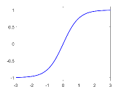
(a) Tanh fucntion

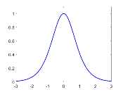
(b) 1st-order derivative of tanh

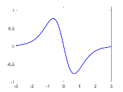
(c) 2nd-order derivative of tanh

Figure 2: The tanh function and its 1st-order and 2nd-order derivatives, respectively

On the other hand, it is significant to initialize the weights and biases of the ELM model. Generally, the weights and biases were initialized according to a uniform distribution. Some works are made to study the value distribution of the internal weights and biases for hidden nodes [50, 51]. In addition, we further investigate the effect of normal distribution initialization on our CELM model and the choice of standard deviation for this initialization approach.

4 Numerical experiments

4.1 Training setup

In this section, we apply the proposed CELM algorithm to solve the biharmonic equation (1.1) in both two and three-dimensional spaces. Two criteria are provided to evaluate the approximation error for our CELM model with different initialization methods and activation functions. They are:

$$APE(\bm{x}^{i})=|\tilde{u}(\bm{x}^{i})-u^{*}(\bm{x}^{i})|~{}~{}\text{and}~{}~{}REL=\sqrt{\frac{\sum_{i=1}^{N^{\prime}}|\tilde{u}(\bm{x}^{i})-u^{*}(\bm{x}^{i})|^{2}}{\sum_{i=1}^{N^{\prime}}|u^{*}(\bm{x}^{i})|^{2}}},$$

where $\tilde{u}(\bm{x}^{i})$ and $u^{*}(\bm{x}^{i})$ are the approximate solution of CELM and exact solution, respectively, for collection points $\{\bm{x}^{i}\}(i=1,2,\cdots,N^{\prime})$, and $N^{\prime}$ represents the number of collection points. We perform all neural networks in Numpy (version 1.21.0) on a workstation (256 GB RAM, single NVIDIA GeForce RTX 4090Ti 24-GB).

4.2 Numerical examples

Example 4.1.

To start, we aim to approximate the solution to the biharmonic equation (1.1) within the regular domain $\Omega=[-1,1]\times[-1,1]$. An analytical solution and a force term are given by

$$u(x_{1},x_{2})=\sin(\pi x_{1})\sin(\pi x_{2})$$

and

$$f(x_{1},x_{2})=4\pi^{4}\sin(\pi x_{1})\sin(\pi x_{2}),$$

respectively. The boundary constraints function $g(x_{1},x_{2})=0$ and $h(x_{1},x_{2})=0$, respectively, on $\partial\Omega$.

In this example, we approximate the solution of (1.1) by the CELM model with 1000 hidden units on 16384 grid points in the domain $[-1,1]\times[-1,1]$ with mesh-size $h=1/128$. Apart from the grid points, the training set also includes 10,000 random points sampled from the interior of $\Omega$ and 4,000 points randomly sampled from four boundary lines of $\Omega$. Firstly, we perform the proposed CELM algorithm on these collections, the internal parameters(weights and biases) are initialized by a scale uniform distribution initialization in $[-10,10]$. The numerical results are plotted in Fig. 3 when activation functions are set as tanh, gaussian, sin, and trigonometric functions sin+cos, respectively. Secondly, the comparative results of different initialization methods including normal distribution initialization with mean zero and a standard deviation 10, unitary uniform distribution initialization in $[-1,1]$, scale uniform distribution initialization, and mixed initialization are listed in Table 1. Finally, the curves of the relative error and the running time vary from the hidden nodes, and the curve of the relative error varies from the standard deviation are depicted in Figure 4 for scale uniform distribution initialization and sine activation function.

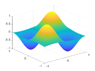
(a) Analytical solution

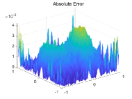
(b) Point-wise error(Tanh)

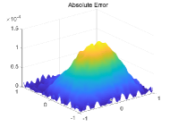
(c) Point-wise error(Gauss)

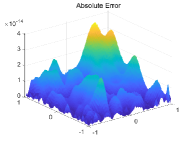
(d) Point-wise error(Sin)

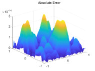
(e) Point-wise error(Sin+Cos)

Figure 3: Numerical results to CELM with scale uniform initialization for Example 4.1.

Table 1: REL of CELM with various activation functions and initialization of parameters for Example 4.1

Init Weight	Normal	Unitary uniform	Scale uniform	Normal
Init Bias	Normal	Unitary uniform	Scale uniform	Scale uniform
Tanh	0.0071	$1.7823\times 10^{-9}$	$3.0943\times 10^{-6}$	$1.2773\times 10^{-4}$
Gauss	$0.0621$	$8.2273\times 10^{-11}$	$1.0937\times 10^{-4}$	0.0027
Sin	$1.7446\times 10^{-13}$	$1.5469\times 10^{-4}$	$2.5259\times 10^{-14}$	$5.9478\times 10^{-14}$
Sin+Cos	$5.8946\times 10^{-14}$	$2.7601\times 10^{-4}$	$2.0427\times 10^{-14}$	$5.2089\times 10^{-14}$

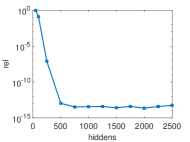
(a) Rel VS the hidden nodes

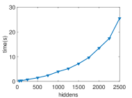
(b) Running time VS the hidden nodes

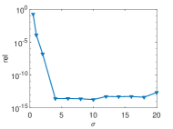
(c) Rel VS the standard deviation $\sigma$

Figure 4: Rel VS the hidden nodes(Left), running time VS the hidden nodes(middle) and Rel VS the standard deviation(right) to CELM model with scale uniform initialization and sin activation function for Example 4.1.

Based on the distribution of point-wise absolute error in Figures 3(a) – 3(e), we can conclude that the CELM models with sin and sin+cos are superior to the ones with tanh and gaussian, and the performance of the CELM model with sin can compete against the one with sin+cos. The data in Table 1 shows that the CELM models with scale uniform initialization perform best for sin and sin+cos activation functions. They outperform other cases by at least three orders of magnitude in terms of the activation function and the initialization method of the hidden unit. According to the curves in Figure 4(a), the relative error will not decrease when the number of hidden units increases, which means the performance of the CELM model with the aforementioned setups trends to be stable with the increasing of hidden neurons. The time-neuron curve in Figure 4(b) shows that the run time will superlinear increase with the increasing of hidden neurons, but its rising tendency is slow. Finally, Figure 4(c) indicates the CELM model is stable and robust for the varying standard deviation. In sum, our CELM method not only has high accuracy but also is efficient and robust.

Example 4.2.

We consider the following biharmonic equation (1.1) in two-dimensional space and obtain its numerical solution within a hexagram domain $\Omega$, which is derived from the $[0,1]\times[0,1]$. An analytical solution and a force collection are given by

$$u(x_{1},x_{2})=10(x_{1}-2x_{1}^{3}+x_{1}^{4})(x_{2}-2x_{2}^{3}+x_{2}^{4})$$

and

$$f(x_{1},x_{2})=240(x_{1}-2x_{1}^{3}+x_{1}^{4})+2880x_{1}x_{2}(x_{1}-1)(x_{2}-1)+240(x_{2}-2x_{2}^{3}+x_{2}^{4}),$$

respectively. The boundary functions $g(x_{1},x_{2})$ can be easily obtained from the exact solution, but for brevity, we will omit them here. By careful calculation, we have the function $h(x_{1},x_{2})$ on $\partial\Omega$, it is

$$h(x_{1},x_{2})=10(-12x_{1}+12x_{1}^{2})(x_{2}-2x_{2}^{3}+x_{2}^{4})+10(x_{1}-2x_{1}^{3}+x_{1}^{4})(-12x_{2}+12x_{2}^{2})$$

In this example, the setups of CELM models are the same as the Example 4.1. One can obtain an approximation for the solution of (1.1) by our proposed CELM algorithm on 20,000 points randomly sampled from the hexagon domain $\Omega$. We plot and list the numerical results in Figs. 5 and 6 as well as Table 2.

(a) Analytical solution

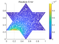
(b) Point-wise error(Tanh)

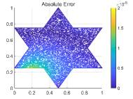
(c) Point-wise error(Gauss)

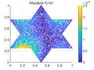
(d) Point-wise error(Sin)

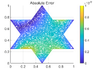
(e) Point-wise error(Sin+Cos)

Figure 5: Numerical results to CELM with scale uniform initialization for Example 4.2.

Table 2: REL of CELM with various activation functions and initialization of parameters for Example 4.2

Init Weight	Normal	Unitary uniform	Scale uniform	Normal
Init Bias	Normal	Unitary uniform	Scale uniform	Scale uniform
Tanh	$7.8642\times 10^{-4}$	$9.0761\times 10^{-9}$	$3.0579\times 10^{-5}$	0.0011
Gauss	0.0321	$4.6728\times 10^{-9}$	$5.0337\times 10^{-6}$	0.0055
Sin	$1.9411\times 10^{-8}$	$2.2124\times 10^{-8}$	$8.9321\times 10^{-10}$	$5.0643\times 10^{-9}$
Sin+Cos	$5.7731\times 10^{-9}$	$4.1012\times 10^{-9}$	$6.0818\times 10^{-10}$	$7.3112\times 10^{-9}$

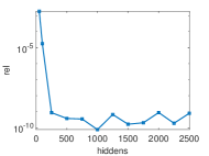
(a) Rel VS the hidden nodes

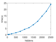
(b) Running time VS the hidden nodes

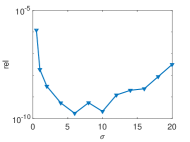
(c) Rel VS the standard deviation $\sigma$

Figure 6: Rel VS the hidden nodes(Left), running time VS the hidden nodes(middle) and Rel VS the standard deviation(right) to CELM model with scale uniform initialization and sin activation function for Example 4.2

Based on the results in Fig. 5 and Table 2, the CELM model with sin activation function, on the irregular domain in two-dimensional space, still possesses the capacity to obtain a satisfactory approximation for the solution of (1.1) when the internal parameters of hidden units are initialized by the scale uniform initialization technique, and its performance is superior to that of the ones with other setups. The curves of relative error and running time in Fig. 6 demonstrate this CELM model is stable and robust for both the varying number of hidden nodes and the varying standard deviation.

Example 4.3.

We consider the following biharmonic equation (1.1) in three-dimensional space and obtain its numerical solution within a unit cubic domain $\Omega=[0,1]\times[0,1]\times[0,1]$. An exact solution is given by

$$u(x_{1},x_{2},x_{3})=10(x_{1}-2x_{1}^{3}+x_{1}^{4})(x_{2}-2x_{2}^{3}+x_{2}^{4})(x_{3}-2x_{3}^{3}+x_{3}^{4}),$$

it will naturally lead to the essential boundary function $g(x_{1},x_{2},x_{3})$, and the function of $h(x_{1},x_{2},x_{3})$ is

$$h(x_{1},x_{2},x_{3}) =10(-12x_{1}+12x_{1}^{2})(x_{2}-2x_{2}^{3}+x_{2}^{4})(x_{3}-2x_{3}^{3}+x_{3}^{4})+10(x_{1}-2x_{1}^{3}+x_{1}^{4})(-12x_{2}+12x_{2}^{2})(x_{3}-2x_{3}^{3}+x_{3}^{4})$$

$$+10(x_{1}-2x_{1}^{3}+x_{1}^{4})(x_{2}-2x_{2}^{3}+x_{2}^{4})(-12x_{3}+12x_{3}^{2}).$$

By performing careful calculations, one can determine the expression for the force side, it is

$$f(x_{1},x_{2},x_{3}) =240x_{2}(1-2x_{2}^{2}+x_{2}^{3})x_{3}(1-2x_{3}^{2}+x_{3}^{3})+240x_{1}(1-2x_{1}^{2}+x_{1}^{3})x_{3}(1-2x_{3}^{2}+x_{3}^{3})$$

$$+240x_{1}(1-2x_{1}^{2}+x_{1}^{3})x_{2}(1-2x_{2}^{2}+x_{2}^{3})+2880x_{1}(x_{1}-1)x_{2}(x_{2}-1)x_{3}(1-2x_{3}^{2}+x_{3}^{3})$$

$$+2880x_{1}(x_{1}-1)x_{3}(x_{3}-1)x_{2}(1-2x_{2}^{2}+x_{2}^{3})+2880x_{2}(x_{2}-1)x_{3}(x_{3}-1)x_{2}(1-2x_{2}^{2}+x_{2}^{3})$$

In this example, we obtain the numerical solution of (1.1) by the CELM model with 2000 hidden units in $\Omega$, the other setups of the CELM model are the same as the Example 4.1. A testing set consists of 16384 grid points in the $xoy$ cutting plane $[0,1]\times[0,1]$ with mesh-size $h=1/128$ when $z=0.5$. Apart from those grid points, the training set includes 10000 random collections sampled from the domain $\Omega$ and 6000 points randomly sampled from six boundaries. We plot and list the numerical results in Figs. 7 and 8 as well as Table 3.

(a) Analytical solution

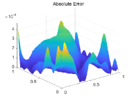
(b) Point-wise error(Tanh)

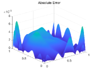
(c) Point-wise error(Gauss)

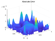
(d) Point-wise error(Sin)

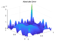
(e) Point-wise error(Sin+Cos)

Figure 7: Numerical results to CELM with scale uniform initialization for Example 4.3.

Table 3: REL of CELM with various activation functions and initialization of parameters for Example 4.3

Init Weight	Normal	Unitary uniform	Scale uniform	Normal
Init Bias	Normal	Unitary uniform	Scale uniform	Scale uniform
Tanh	0.0051	$7.1068\times 10^{-8}$	$2.7657\times 10^{-4}$	0.0051
Gauss	0.3977	$605164\times 10^{-9}$	0.0047	0.2498
Sin	$1.5912\times 10^{-9}$	0.0022	$9.4702\times 10^{-13}$	$1.3471\times 10^{-9}$
Sin+Cos	$1.6214\times 10^{-9}$	0.0015	$1.0059\times 10^{-12}$	$4.7209\times 10^{-10}$

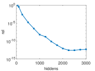
(a) Rel VS the hidden nodes

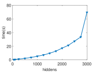
(b) Running time VS the hidden nodes

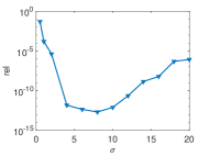
(c) Rel VS the standard deviation $\sigma$

Figure 8: Rel VS the hidden nodes(Left), running time VS the hidden nodes(middle) and Rel VS the standard deviation(right) to CELM model with scale uniform initialization and sin activation function for Example 4.3.

Based on the point-wise error in Figs. 7(b) – 7(e), our proposed CELM model with sin and sin+cos are also able greatly to solve the biharmonic equation (1.1) in three-dimensional space when the internal parameters of hidden units are initialized by the scale uniform initialization technique. The relative errors in Table 3 reveal the CELM model with the configurations above outperforms the ones with other setups. The curves of relative error and running time in Fig. 8 demonstrate the CELM model has favourable stability and robustness when the number of hidden nodes and the standard deviation are both increased.

Example 4.4.

We consider the following biharmonic equation (1.1) in there-dimensional space and obtain its numerical solution on a closed domain $\Omega$ restrained by two spherical surfaces with radius $r_{1}=0.5$ and $r_{2}=1.0$, respectively. The exact solution is given by

$$u(x_{1},x_{2},x_{3})=\sin(\pi x_{1})\sin(\pi x_{2})\sin(\pi x_{3}),$$

it will naturally lead to the determination of the boundary conditions $g(x_{1},x_{2},x_{3})$ and $h(x_{1},x_{2},x_{3})$ on $\partial\Omega$, they are:

$$\begin{cases}g(x_{1},x_{2},x_{3})=\sin(\pi x_{1})\sin(\pi x_{2})\sin(\pi x_{3}),\\ h(x_{1},x_{2},x_{3})=-3\pi^{2}\sin(\pi x_{1})\sin(\pi x_{2})\sin(\pi x_{3}),\end{cases}$$

respectively. By carefully calculations, one can obtain the force side $f(x_{1},x_{2},x_{3})=9\pi^{4}\sin(\pi x_{1})\sin(\pi x_{2})\sin(\pi x_{3})$.

In this example, we obtain the numerical solution of (1.1) by the CELM model with 2000 hidden units in $\Omega$, the other setups of the CELM model are the same as the Example 4.1. The testing set consists of 3000 mesh grid points on the spherical surface with radius $r=0.8$. Apart from the mesh-grid points, the training set also includes 40000 points sampled randomly from the domain $\Omega$ and 20,000 random points sampled equally from the inner and the outer spherical surface, respectively. We plot and listed the numerical results in Fig. 9 and 10 as well as Table 4.

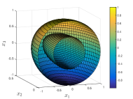
(a) Domain

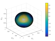
(b) Analytical solution

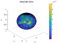
(c) Point-wise error(Tanh)

(d) Point-wise error(Gauss)

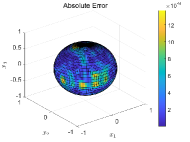
(e) Point-wise error(Sin)

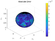
(f) Point-wise error(Sin+Cos)

Figure 9: Numerical results to CELM with scale uniform initialization for Example 4.4.

Table 4: REL of CELM with various activation activations and initialization of parameters for Example 4.4

Init Weight	Normal	Unitary uniform	Scale uniform	Normal
Init Bias	Normal	Unitary uniform	Scale uniform	Scale uniform
Tanh	0.0781	$2.5835\times 10^{-8}$	$0.0046$	0.0391
Gauss	0.3527	$2.1657\times 10^{-9}$	0.0561	0.3491
Sin	$1.4873\times 10^{-5}$	0.0037	$9.5917\times 10^{-9}$	$2.1146\times 10^{-5}$
Sin+Cos	$2.0745\times 10^{-5}$	0.0027	$5.3452\times 10^{-9}$	$1.3402\times 10^{-5}$

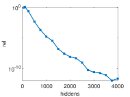
(a) Rel VS the hidden nodes

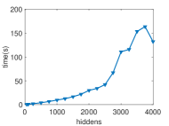
(b) Running time VS the hidden nodes

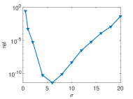
(c) Rel VS the standard deviation $\sigma$

Figure 10: Rel VS the hidden nodes(Left), running time VS the hidden nodes(middle) and Rel VS the standard deviation(right) to CELM model with scale uniform initialization and sin activation function for Example 4.4.

For the sphere cavity in three-dimensional space, the point-wise errors in Figs. 9(c) – 9(f) manifest our proposed CELM model with sin and sin+cos are less than that of the ones with tanh and gaussian to solve the biharmonic equation (1.1) when the internal parameters of hidden units are initialized by the scale uniform initialization technique. Table 4 shows that the CELM model with the specified configurations outperforms those with other setups, as evidenced by the lower relative errors. Additionally, the curves of relative error and running time in Fig.10 demonstrate the CELM model’s favourable stability and robustness when the number of hidden nodes and the standard deviation are varied.

5 Conclusion

We have proposed a coupled extreme learning machine to solve the biharmonic problems by embracing the splitting scheme of the biharmonic equation with the simple ELM network. Similar to other networks, such as the PINN and radius basis function model, the CELM model is also devoid of mesh and does not depend on an initial guess. Unlike the PINN structure, the CELM is an efficient method for approximating the solution of (1.1) without the requirement of parameter update by iterative gradient descent-based technique. Additionally, the influence of activation functions including tanh, gaussian, sin and sin+cos are studied for the CELM model, the investigations are carried out on the initialization of internal parameters for hidden units. The computational results provide evidence that the proposed method is highly accurate and efficient in solving (1.1) in both regular and irregular domains. Our current work entails expanding neural network models to address additional high-order partial differential equations in the future.

Contributions

Xi’an Li: Conceptualization, Methodology, Investigation, Validation, Software and Writing - Original Draft; Jinran Wu: Conceptualization, Writing - review $\&$ editing; Jiaxin Deng: Software and Writing - review $\&$ editing; Zhe Ding: Conceptualization, Writing - review $\&$ editing; You-Gan Wang: Writing - Review & Editing; Xin Tai: Writing - Review & Editing; Liang Liu: Writing - Review & Editing. All authors have read and agreed to the published version of the manuscript.

Declaration of interests

All authors declare that they have no known competing financial interests or personal relationships that could have appeared to influence the work reported in this paper.

References

- Wahba [1990] G. Wahba, Spline models for observational data, 1990.
- Greengard and Kropinski [1998] L. Greengard, M. C. Kropinski, An integral equation approach to the incompressible navier–stokes equations in two dimensions, SIAM Journal on Scientific Computing 20 (1998) 318–336.
- Ferziger and Peric [1996] J. H. Ferziger, M. Peric, Computational methods for fluid dynamics, 1996.
- Christiansen [1975] S. Christiansen, Integral equations without a unique solution can be made useful for solving some plane harmonic problems, Ima Journal of Applied Mathematics 16 (1975) 143–159.
- Constanda [1995] C. Constanda, The boundary integral equation method in plane elasticity, Proceedings of the American Mathematical Society 123 (1995) 3385–3396.
- Gupta and Manohar [1979] M. M. Gupta, R. P. Manohar, Direct solution of the biharmonic equation using noncoupled approach, Journal of Computational Physics 33 (1979) 236–248.
- Altas et al. [1998] I. Altas, J. Dym, M. M. Gupta, R. P. Manohar, Multigrid solution of automatically generated high-order discretizations for the biharmonic equation, SIAM Journal on Scientific Computing 19 (1998) 1575–1585.
- Ben-Artzi et al. [2008] M. Ben-Artzi, J.-P. Croisille, D. Fishelov, A fast direct solver for the biharmonic problem in a rectangular grid, SIAM Journal on Scientific Computing 31 (2008) 303–333.
- Bialecki [2012] B. Bialecki, A fourth order finite difference method for the dirichlet biharmonic problem, Numerical Algorithms 61 (2012) 351–375.
- Chun-jiaBi and Li-kangLi [2004] Chun-jiaBi, Li-kangLi, Mortar finite volume method with adini element for biharmonic problem, Journal of Computational Mathematics 22 (2004) 475–488.
- Wang [2004] T. Wang, A mixed finite volume element method based on rectangular mesh for biharmonic equations, Journal of Computational and Applied Mathematics 172 (2004) 117–130.
- Eymard et al. [2012] R. Eymard, T. Gallouët, R. Herbin, A. Linke, Finite volume schemes for the biharmonic problem on general meshes, Mathematics of Computation 81 (2012) 2019–2048.
- Baker [1977] G. A. Baker, Finite element methods for elliptic equations using nonconforming elements, Math Comp (1977).
- Lascaux and Lesaint [1975] P. Lascaux, P. Lesaint, Some nonconforming finite elements for the plate bending problem, Revue Franaise Dautomatique Informatique Recherche Opérationnelle Analyse Numérique (1975).
- Morley [2016] L. S. D. Morley, The triangular equilibrium element in the solution of plate bending problems, Aeronautical Quarterly 19 (2016).
- Zienkiewicz et al. [2005] O. C. Zienkiewicz, R. L. Taylor, P. Nithiarasu, The finite element method for fluid dynamics, Elsevier Butterworth-Heinemann,, 2005.
- Ciarlet and Oden [1978] P. G. Ciarlet, J. T. Oden, The Finite Element Method for Elliptic Problems, 1978.
- Smith [1968] J. Smith, The coupled equation approach to the numerical solution of the biharmonic equation by finite differences. ii, SIAM Journal on Numerical Analysis 5 (1968) 104–111.
- Ehrlich [1971] L. W. Ehrlich, Solving the biharmonic equation as coupled finite difference equations, SIAM Journal on Numerical Analysis 8 (1971) 278–287.
- Brezzi and Fortin [1991] F. Brezzi, M. Fortin, Mixed and hybrid finite element methods, 1991.
- Cheng et al. [2000] X.-L. Cheng, W. Han, H. ci Huang, Some mixed finite element methods for biharmonic equation, Journal of Computational and Applied Mathematics 126 (2000) 91–109.
- Davini [2000] C. Davini, An unconstrained mixed method for the biharmonic problem, SIAM Journal on Numerical Analysis 38 (2000) 820–836.
- Lamichhane [2011] B. P. Lamichhane, A stabilized mixed finite element method for the biharmonic equation based on biorthogonal systems, Journal of Computational and Applied Mathematics 235 (2011) 5188–5197.
- Stein et al. [2019] O. Stein, E. Grinspun, A. Jacobson, M. Wardetzky, A mixed finite element method with piecewise linear elements for the biharmonic equation on surfaces., arXiv preprint arXiv:1911.08029 (2019).
- Mai-Duy et al. [2009] N. Mai-Duy, H. See, T. Tran-Cong, A spectral collocation technique based on integrated chebyshev polynomials for biharmonic problems in irregular domains, Applied Mathematical Modelling 33 (2009) 284–299.
- Bialecki and Karageorghis [2010] B. Bialecki, A. Karageorghis, Spectral chebyshev collocation for the poisson and biharmonic equations, SIAM Journal on Scientific Computing 32 (2010) 2995–3019.
- Bialecki et al. [2020] B. Bialecki, G. Fairweather, A. Karageorghis, J. Maack, A quadratic spline collocation method for the dirichlet biharmonic problem, Numerical Algorithms 83 (2020) 165–199.
- Mai-Duy and Tanner [2005] N. Mai-Duy, R. Tanner, An effective high order interpolation scheme in biem for biharmonic boundary value problems, Engineering Analysis With Boundary Elements 29 (2005) 210–223.
- Adibi and Es’haghi [2007] H. Adibi, J. Es’haghi, Numerical solution for biharmonic equation using multilevel radial basis functions and domain decomposition methods, Applied Mathematics and Computation 186 (2007) 246–255.
- Li et al. [2011] X. Li, J. Zhu, S. Zhang, A meshless method based on boundary integral equations and radial basis functions for biharmonic-type problems, Applied Mathematical Modelling 35 (2011) 737–751.
- Guo et al. [2019] H. Guo, X. Zhuang, T. Rabczuk, A deep collocation method for the bending analysis of kirchhoff plate, Cmc-computers Materials and Continua 59 (2019) 433–456.
- Huang et al. [2021] Z. Huang, S. Chen, W. Chen, L. Peng, Neural network method for thin plate bending problem, Chinese Journal of Solid Mechanics 42 (2021) 10.
- Vahab et al. [2022] M. Vahab, E. Haghighat, M. Khaleghi, N. Khalili, A physics-informed neural network approach to solution and identification of biharmonic equations of elasticity, Journal of Engineering Mechanics 148 (2022) 04021154.
- Samaniego et al. [2020] E. Samaniego, C. Anitescu, S. Goswami, V. Nguyen-Thanh, H. Guo, K. Hamdia, X. Zhuang, T. Rabczuk, An energy approach to the solution of partial differential equations in computational mechanics via machine learning: Concepts, implementation and applications, Computer Methods in Applied Mechanics and Engineering 362 (2020) 112790.
- Li et al. [2021] W. Li, M. Z. Bazant, J. Zhu, A physics-guided neural network framework for elastic plates: Comparison of governing equations-based and energy-based approaches, Computer Methods in Applied Mechanics and Engineering 383 (2021) 113933.
- Guo and Zhuang [2021] H. Guo, X. Zhuang, The application of deep collocation method and deep energy method with a two-step optimizer in the bending analysis of kirchhoff thin plate, Chinese Journal of Solid Mechanics 42 (2021) 18.
- Li et al. [2022] X. Li, J. Wu, L. Zhang, X. Tai, Solving a class of high-order elliptic pdes using deep neural networks based on its coupled scheme, Mathematics 10 (2022) 4186.
- Dwivedi and Srinivasan [2020a] V. Dwivedi, B. Srinivasan, Physics informed extreme learning machine (pielm)–a rapid method for the numerical solution of partial differential equations, Neurocomputing 391 (2020a) 96–118.
- Dwivedi and Srinivasan [2020b] V. Dwivedi, B. Srinivasan, Solution of biharmonic equation in complicated geometries with physics informed extreme learning machine, Journal of Computing and Information Science in Engineering 20 (2020b) 061004.
- Li et al. [2023] S. Li, G. Liu, S. Xiao, Extreme learning machine with kernels for solving elliptic partial differential equations, Cognitive Computation 15 (2023) 413–428.
- Wang and Dong [2023] Y. Wang, S. Dong, An extreme learning machine-based method for computational pdes in higher dimensions, arXiv preprint arXiv:2309.07049 (2023).
- Pao et al. [1994] Y.-H. Pao, G.-H. Park, D. J. Sobajic, Learning and generalization characteristics of the random vector functional-link net, Neurocomputing 6 (1994) 163–180.
- Liu et al. [2021] F. Liu, X. Huang, Y. Chen, J. A. Suykens, Random features for kernel approximation: A survey on algorithms, theory, and beyond, IEEE Transactions on Pattern Analysis and Machine Intelligence 44 (2021) 7128–7148.
- Chen et al. [2022] J. Chen, X. Chi, Z. Yang, et al., Bridging traditional and machine learning-based algorithms for solving pdes: The random feature method, arXiv preprint arXiv:2207.13380 (2022).
- Sun and Wang [2023] J. Sun, F. Wang, Local randomized neural networks with discontinuous galerkin methods for diffusive-viscous wave equation, arXiv preprint arXiv:2305.16060 (2023).
- Adriazola [2022] J. Adriazola, On the role of tikhonov regularizations in standard optimization problems, arXiv preprint arXiv:2207.01139 (2022).
- Fabiani et al. [2021] G. Fabiani, F. Calabrò, L. Russo, C. Siettos, Numerical solution and bifurcation analysis of nonlinear partial differential equations with extreme learning machines, Journal of Scientific Computing 89 (2021) 1–35.
- Calabrò et al. [2021] F. Calabrò, G. Fabiani, C. Siettos, Extreme learning machine collocation for the numerical solution of elliptic pdes with sharp gradients, Computer Methods in Applied Mechanics and Engineering 387 (2021) 114188.
- Ma et al. [2022] M. Ma, J. Yang, R. Liu, A novel structure automatic-determined fourier extreme learning machine for generalized black–scholes partial differential equation, Knowledge-Based Systems 238 (2022) 107904.
- Dong and Yang [2022] S. Dong, J. Yang, On computing the hyperparameter of extreme learning machines: Algorithm and application to computational pdes, and comparison with classical and high-order finite elements, Journal of Computational Physics 463 (2022) 111290.
- Quan and Huynh [2023] H. D. Quan, H. T. Huynh, Solving partial differential equation based on extreme learning machine, Mathematics and Computers in Simulation 205 (2023) 697–708.