Nested solutions of gravitational condensate stars

Abstract

Black holes are normally and naturally associated to the end-point of gravitational collapse. Yet, alternatives have been proposed and a particularly interesting one is that of gravitational condensate stars, or gravastars [1]. We here revisit the gravastar model and increase the degree of speculation by considering new solutions that are inspired by the original model of gravastars with anisotropic pressure, but also offer surprising new features. In particular, we show that it is possible to nest two gravastars into each other and obtain a new solution of the Einstein equations. Since each gravastar essentially behaves as a distinct self-gravitating equilibrium, a large and rich space of parameters exists for the construction of nested gravastars. In addition, we show that these nested-gravastar solutions can be extended to an arbitrarily large number of shells, with a prescription specified in terms of simple recursive relations. Although these ultra-compact objects are admittedly very exotic, some of the solutions found, provide an interesting alternative to a black hole by having a singularity-free origin, a full matter interior, a time-like matter surface, and a compactness $\mathcal{C}\to(1/2)^{-}$.

1 Introduction

Despite the compelling evidence that black holes are perfectly compatible with gravitational-wave [2] and electromagnetic [3, 4] observations, their physical existence – and the conceptual consequences of such an existence – still represents a challenge for modern physics. Because of this, a vast literature about compact astrophysical objects with properties similar to those of black holes has been developed over the last decades (see, e.g.,  [5] for a review). It is within this large body of works that the ingenious solution of Mazur and Mottola [1, 6] was proposed in 2001 as the endpoint of gravitational collapse and an alternative to the Schwarzschild solution [7].

The gravitational vacuum condensate star, or “gravastar”, proposed by Mazur and Mottola comprises an infinitesimally thin shell with the most extreme and causal equation of state (EOS) for the (isotropic) pressure $p$ as a function of the energy density $e$ [8], namely, $p=e$, and a de-Sitter interior with an EOS with $p=-e$, which is interpreted as dark energy and is often invoked as a natural explanation of the accelerated expansion of the universe, where it appears as a cosmological constant. The latter EOS has a long history, starting from 1966, when Sakharov concluded that it can arise when an isolated gravitating system reaches large baryon densities [9]. In the same year, Gliner [10] suggested that such a dark-energy state of matter with a de-Sitter metric [11] might represent the final state of gravitational collapse. From an intuitive point of view, while the negative pressure from the de-Sitter region seeks to expand the gravastar, the thin shell with an ultra-stiff EOS counterbalances the expansion leading to a static but nonvacuum solution of the Einstein equations in spherical symmetry. Less extreme EOSs are possible if the thin shell is replaced by a thick one and an anisotropic pressure is added (see, e.g.,  [12]). The gravastar model is not alone in the category of nonsingular black holes. Important work in this regard has been carried out by Dymnikova [14, 15, 16], while a remarkable connection between the gravastar and the constant-density interior Schwarzschild solution has been identified by Mazur and Mottola [17].

There are several advantages behind a gravastar solution. First, it provides the endpoint of gravitational collapse without the central spacelike singularity encountered in the Schwarzschild solution. Second, it removes altogether the problem of an information paradox, since the gravastar surface can be placed infinitesimally outside the putative event horizon and thus is not a null but a time-like surface (compact objects of this type are often referred to as “nonsingular and horizon-less” black holes). Indeed, in the case of gravastars, the Buchdahl bound [18] for the compactness of spherically symmetric objects, can be easily avoided through the introduction of anisotropic transverse stresses, resulting in a gravastar within the framework of the interior Schwarzschild solution [17]. While an isolated gravastar would be very hard to distinguish from a black hole when employing electromagnetic radiation (see, e.g.,  [19]), the response to gravitational perturbations is different, thus making gravastars distinguishable from black holes when measuring their ringdown signal [12, 20].

At the same time, more then 20 years since their introduction, the genesis of gravastars is still highly speculative and fundamentally unclear even in the most idealised conditions. It is claimed that quantum fluctuations amplified during the final stages of the collapse induce a vacuum phase transition, yielding the emergence of dark energy and enabling the formation of the shell [21]. However, realistic calculations demonstrating that this process is dynamically possible are still lacking; in addition, the astrophysical evidence of their existence is also shrouded by doubts [22, 20, 23]. However, because the considerations that we will present here are even more speculative than those that normally accompany gravastars, we will indulge on ignoring the complications associated with the creation of gravastars and simply assume that these solutions are not only mathematically possible but also realisable in nature.

We here continue the exploration of static and spherically symmetric gravitational condensate stars by increasing the degree of speculation and constructing a new solution consisting of two gravastars nested into each other. Again, from an intuitive point of view, it is natural to expect that since each of the two gravastars is already in a near hydrostatic equilibrium, the nesting of the two solutions can lead to yet another static equilibrium. In practice, we show that a suitable but generic prescription for the EOS of the matter in the two shells provides a solution of the Einstein equations for two nested gravastars, namely a “nestar”. Intrigued by this behaviour, we explore the possibility of nesting an additional gravastar and show that this is also possible, leading in fact to a precise recipe for introducing an arbitrary number of nested gravastars. Hence, in the limit of infinite nested shells it is possible to construct a nonvacuum, nonsingular, static and matter-filled interior of a compact object whose compactness can reach values arbitrarily close to the Schwarzschild limit.

The structure of the paper is as follows. We begin in Sec. 2 with a concise overview of the Mazur-Mottola thin-shell gravastar model and discuss in Sec. 3 how it can be extended by removing the assumption of an infinitesimal shell and by introducing a finite-size shell with a continuous and anisotropic pressure profile. Section 4 is instead dedicated to the analysis of nested solutions of gravastars for which we can ensure continuity conditions for all relevant spacetime and fluid functions and their first derivatives. We also explore the rich space of parameters and solutions that can be obtained when varying the thickness and compactness of the matter shells. We derive expressions that can be cast in terms of generic coefficients that follow recurrent relations that we collect in Appendix 6, where we also discuss the rich radial structure of a “nestar”. Finally, Sec. 5 summarises our results and suggests possible developments.

2 Gravastars with isotropic pressure (thin shell)

Before entering the details of the new nested-gravastars model, it is useful to briefly recall the thin-shell gravastar model proposed by Mazur and Mottola [1, 6]. Let us start from a generic, static and spherically symmetric line element in the form

$$ds^{2}=-f(r)dt^{2}+\frac{dr^{2}}{h(r)}+r^{2}(d\theta^{2}+\sin^{2}(\theta)d\phi^{2})\,,$$ (1)

and split the spacetime into three different regions marked by the radial coordinate $r$, namely,

  I.   de-Sitter interior $$r\in\left[0,r_{1}\right)\,,\hskip 28.45274pt p=-e\,,$$ (2)

 II.  matter shell $$r\in\left[r_{1},r_{2}\right]\,, p=e\,,$$ (3)

III.  vacuum exterior $$r\in\left(r_{2},\infty\right)\,, p=e=0\,.$$ (4)

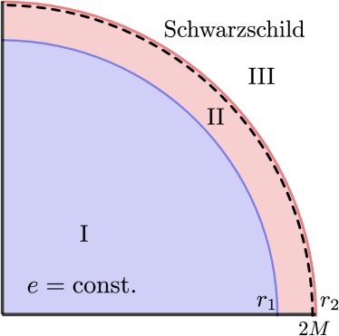
Figure 1: Illustrative representation of a gravastar. Shown with different colours are the three different regions of the spacetime: a de-Sitter region (I., blue-shaded area), the ultra-stiff shell (II., red-shaded area), and the Schwarzschild vacuum exterior (III., white area). Shown with a black dashed line is the position of the surface $r=2M$, with $M$ the mass of the gravastar.

The Einstein equations and the momentum-conservation equation for a perfect fluid at rest take the following form

$$-G^{\,t}_{\,\,t} = \frac{1}{r^{2}}\frac{d}{dr}[r(1-h)] =-8\pi T^{\,t}_{\,\;t} =8\pi e\,,$$ (5)

$$\phantom{-}G^{\,r}_{\,\,r} =\frac{h}{rf} \frac{df}{dr}+\frac{1}{r^{2}}(h-1) =\phantom{-}8\pi T^{\,r}_{\,\;r} =8\pi p\,,$$ (6)

$$\nabla_{i}T^{\,i}_{\,\;r}=\frac{dp}{dr}+\frac{e+p}{2f}\frac{df}{dr}=0\,,$$ (7)

where $G_{\mu\nu}$ and $T_{\mu\nu}$ are the Einstein and energy-momentum tensors, respectively. The solution of Eqs. (5)–(7) leads, in the thin-shell approximation $|1-r_{2}/r_{1}|\ll 1$ and $0<h\ll 1$, to the following metric functions

I. de-Sitter interior: $$\begin{cases}\begin{aligned} f(r)&=C(1-H_{0}^{2}r^{2})\,,\\ \vspace{0.5cm}h(r)&=1-H_{0}^{2}r^{2}\,,\end{aligned}\end{cases}$$ (8)

II. matter shell: $$\begin{cases}\begin{aligned} f(r)&={w_{1}}f(r_{1})/{w(r)}\,,\\ h(r)&=\epsilon\,[1+w(r)]^{2}/w(r)\,,\end{aligned}\end{cases}$$ (9)

III. exterior: $$\begin{cases}\begin{aligned} f(r)&=1-{2M}/{r}\,,\\ h(r)&=1-{2M}/{r}\,,\end{aligned}\end{cases}$$ (10)

where $w(r):=8\pi r^{2}\,p(r)$ is a dimensionless quantity, defined only within the shell, with constants given by $w_{1}:=w(r_{1})$ and $w_{2}:=w(r_{2})$. Enforcing continuity of the metric functions at each layer fixes the free constants in the model, namely

$$\epsilon =-\ln\left(\dfrac{r_{2}}{r_{1}}\right)\left[\,\ln\left(\dfrac{w_{2}}{w_{1}}\right)-\dfrac{1}{w_{2}}+\dfrac{1}{w_{1}}\right]^{-1}\,,$$ (11)

$$C =\biggl{(}\dfrac{1+w_{2}}{1+w_{1}}\biggr{)}^{2}\,,$$ (12)

$$H_{0}^{2} =\dfrac{1}{r_{1}^{2}}\left[1-\epsilon\,\dfrac{(1+w_{1})^{2}}{w_{1}}\right]\,,$$ (13)

$$M =\dfrac{r_{2}}{2}\left[1-\epsilon\,\dfrac{(1+w_{2})^{2}}{w_{2}}\right]\,.$$ (14)

Finally, we make the interesting remark that if we introduce the coordinate transformation

$$r^{*}=e^{\displaystyle\,\tfrac{1}{w_{1}}}\left(\frac{r}{r_{1}}\right)^{\displaystyle\tfrac{1}{\epsilon}}\frac{1}{w_{1}}\,,$$ (15)

then the metric function $w(r)$ is very well approximated analytically by the Lambert $W$ function

$$w(r)={W_{0}(r^{*})}^{-1}\,.$$ (16)

When comparing to numerically computed solutions and allowing for a finite shell thickness, denoting it by $\delta:=r_{2}-r_{1}$ and the mass of the gravastar by $M$, this representation is very accurate in the case of $\delta/M\ll 1$ and maintains a relative error with respect to the numerical solution that is of the order of a couple percent in the case of $\delta/M\simeq 1/2$.

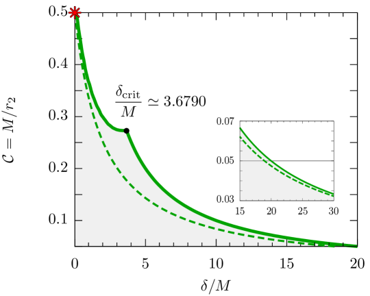
Figure 2: Space of numerical solutions for an isotropic-pressure gravastar shown as a function of the gravastar compactness $\mathcal{C}:=M/r_{2}$ and of the shell thickness $\delta:=r_{2}-r_{1}$. The solutions are found by fixing $r_{2}$ and then varying the inner radius $r_{1}$ and the de-Sitter energy density, which yield either high-compactness, thin-shell gravastars, or low-compactness, thick-shell gravastars. The solid green line marks the edge of the space of solutions beyond which an event horizon appears or the radius $r_{1}<0$, with the critical shell thickness $\delta_{\rm crit}$ denoting the boundary between the two different branches of the limit. A smaller space of solutions was found in Ref. [12] and its limit is marked with a green dashed line; the two limits coincide when $\delta\to 0$ and $\delta\to\infty$, as shown in the small inset. Shown with a red asterisk is the isotropic-pressure (thin-shell) gravastar solution.

2.1 Space of solutions of isotropic-pressure gravastars

In order to explore the space of possible solutions of isotropic-pressure gravastars, we will not only use the analytic thin-shell solution, but also include solutions having a finite-thickness shell, which are computed numerically, using the same EOSs in Eqs. (2)–(4). Imposing that an event horizon is not produced is equivalent to imposing that the metric functions must remain positive. We therefore start by fixing the position of the outer radius $r_{2}$, then set a maximum value for the de-Sitter energy density and start an iteration process over all possible values of $r_{1}$ and de-Sitter energy densities, checking for sign changes in the metric functions and saving as admissible those configurations for which this change in sign does not occur.

Figure 2 reports with a grey-shaded area the space of allowed solutions when expressed in terms of the shell thickness $\delta$, and of the gravastar compactness, i.e., $\mathcal{C}:=M/r_{2}$. The limit of the space of solutions is marked with a solid green line and marks the location where $g_{tt}=0$, hence the appearance of an event horizon, or where $r_{1}=0$. Note that the edge of the region of allowed solutions is characterised by a critical shell thickness $\delta_{\rm crit}$, which distinguishes two qualitatively different behaviours and hence branches ($\delta_{\rm crit}$ also marks a critical compactness $\mathcal{C}_{\rm crit}\simeq 0.2718$). More specifically, solutions approaching the edge along lines with $\mathcal{C}{\delta}/{M}={\rm const.}<1$ and for which $\delta>\delta_{\rm crit}$, are characterised by the hyperbolic condition

$$\mathcal{C}\frac{\delta}{M}=\frac{r_{2}-r_{1}}{r_{2}}\to 1\qquad\Rightarrow r_{1}\to 0\,,$$ (17)

and represent what we refer to as the “unrestricted branch” of solutions because, once the value for $r_{2}>\delta_{\rm crit}>2M$ is fixed, the inner radius of the shell $r_{1}$ can be taken to be arbitrarily close to zero. On the other hand, solutions approaching the edge but with $\delta<\delta_{\rm crit}$ are such that once the value for $\delta_{\rm crit}>r_{2}>2M$ is fixed, a minimum value for $r_{1}$ appears and is dependent on $r_{2}$; because of this, we refer to this as the “restricted branch”. We note that the space of solutions reported in Fig. 2 differs from the equivalent one shown in Fig. 1 of Ref. [12], whose limit of the space of solutions is shown as a green dashed line. While edges of the two spaces of parameters coincide in the limits of $\delta\to 0$ and $\delta\to\infty$ (see inset in Fig. 2) the space of solutions reported here is larger than in Ref. [12], most likely because the initialisation of the discretisation in the interior radius and of the de-Sitter energy density is finer than that employed in Ref. [12]. Finally, we mark with a red asterisk in Fig. 2 the isotropic-pressure (thin-shell) gravastar solution proposed by Mazur and Mottola [1] as a way to remark that such solution represents a very special (and the most extreme) solution in the space of gravastar solutions.

3 Gravastars with anisotropic pressures (thick shell)

It was realised already early on by Cattoen and Visser that when moving away from the infinitesimally thin-shell gravastar model and introducing a more realistic finite-size shell, the pressure cannot be isotropic [24]. As a result, for such anisotropic-pressure gravastars (or thick-shell gravastars) the shell does not have a simple ultra-stiff EOS $p=e$, but a more involved function $p=p(e)$, which is otherwise arbitrary. Adopting the same notation as in [12], we rewrite the static and spherically symmetric line element (1) as

$$ds^{2}=-e^{\nu(r)}dt^{2}+e^{\lambda(r)}dr^{2}+r^{2}(d\theta^{2}+\sin^{2}(\theta)d\phi^{2})\,,$$ (18)

and consider a perfect fluid stress-energy tensor with a radial pressure $p_{r}$ and a tangential pressure $p_{t}$ given by $T^{\mu}_{\phantom{\mu}\nu}=\textnormal{diag}\left(-e,p_{r},p_{t},p_{t}\right)$. The corresponding nonzero Einstein equations then become

$$e^{-\lambda(r)} =g_{rr}(r)^{-1}=1-\frac{2m(r)}{r}\,,$$ (19)

$$\nu^{\,\prime}(r) =\frac{2m(r)+8\pi r^{3}p_{r}}{r[r-2m(r)]}\,,$$ (20)

$$p_{r}^{\,\prime} =-(e+p_{r})\,\frac{m(r)+4\pi r^{3}p_{r}}{r[r-2m(r)]}+\frac{2(p_{t}-p_{r})}{r}\,,$$ (21)

where, as customary, we have defined the mass function as

$$m(r):=\int_{0}^{r}4\pi r^{2}e(r)\,dr\,,$$ (22)

and used a prime ^′ to indicate the total radial derivative.

3.1 Conditions on the fluid variables

Clearly, at the interfaces between the different regions of the spacetime we wish to impose the continuity of the energy density, its first and second derivative, thus ensuring the corresponding continuity of both the radial pressure (up to the second derivative) and of the tangential pressure (up to the first derivative). This marks a difference with respect to what proposed in  [12], where the continuity of the energy density was ensured only up to the first derivative, thus leading to a discontinuity in the first derivative of the tangential pressure. We therefore enforce

$$e(0)=e(r_{1})=e_{1}\,,\hskip 56.9055pt e(r_{2})=0\,,$$ (23)

$$e^{\prime}(r_{1})=0=e^{\prime}(r_{2})\,, e^{\prime\prime}(r_{1})=0=e^{\prime\prime}(r_{2})\,.$$ (24)

We can easily satisfy these conditions via the following energy-density function

$$e(r)=\left\{\begin{aligned} \vspace{0.1em}&\,e_{1}={\rm const.}&\quad{\rm for}\quad&0\leq r<r_{1}\,,\quad&&\mathrm{:\leavevmode\nobreak\ I.\leavevmode\nobreak\ interior}\,,\\ \vspace{0.1em}&\,\sum^{5}_{i=0}a_{i}\,r^{i}&\quad{\rm for}\quad&r_{1}\leq r\leq r_{2}\,,\quad&&\mathrm{:\leavevmode\nobreak\ II.\leavevmode\nobreak\ shell}\,,\\ \vspace{0.1em}&\quad 0&\quad{\rm for}\quad&r_{2}<r\,,\quad&&\mathrm{:\leavevmode\nobreak\ III.\leavevmode\nobreak\ exterior}\,,\end{aligned}\right.$$ (25)

where the six coefficients $a_{0}-a_{5}$ can be computed after a bit of algebra and are given by

$$a_{5} =-\frac{6e_{1}}{(r_{2}-r_{1})^{5}}\,,\quad a_{4} =\frac{15e_{1}(r_{1}+r_{2})}{(r_{2}-r_{1})^{5}}\,,$$

$$a_{3} =-\frac{10e_{1}(r_{1}^{2}+4r_{1}r_{2}+r_{2}^{2})}{(r_{2}-r_{1})^{5}}\,,\quad a_{2} =\frac{30e_{1}r_{1}r_{2}(r_{1}+r_{2})}{(r_{2}-r_{1})^{5}}\,,$$ (26)

$$a_{1} =-\frac{30e_{1}r_{1}^{2}r_{2}^{2}}{(r_{2}-r_{1})^{5}}\,,\quad a_{0} =\frac{e_{1}r_{2}^{3}(10r_{1}^{2}-5r_{1}r_{2}+r_{2}^{2})}{(r_{2}-r_{1})^{5}}\,.$$

To obtain the de-Sitter interior with constant energy density $e_{1}$ in terms of the total mass $M:=m(r_{2})$ we write

$$e_{1}=\frac{21M}{\pi}\left(5\,r_{1}^{3}+9\,r_{1}^{2}\,r_{2}+9\,r_{1}\,r_{2}^{2}+5\,r_{2}^{3}\right)^{-1}\,.$$ (27)

Next, while the EOS for the radial pressure $p_{r}$ in the interior and exterior follows the prescription of (2) and (4), we employ the EOS for the radial pressure in the shell as suggested in Ref. [25] and which is a nonlinear function of the energy density with both a quadratic and a quartic term, namely,

$$p_{r}(e)=\left(\frac{e^{2}}{e_{1}}\right)\Biggl{[}\alpha-(1+\alpha)\left(\frac{e}{e_{1}}\right)^{2}\Biggr{]}\,,$$ (28)

where the constant $\alpha$ can be constrained by requiring that the sound speed $c_{s}^{2}:=dp_{r}/de$ is always subluminal, which yields

$$\alpha\leq\alpha_{\rm crit}:=\frac{3}{4}\Biggl{[}\sqrt[3]{4-2\sqrt{2}}+\sqrt[3]{2(2+\sqrt{2})}\,\Biggr{]}\simeq 2.2135\,.$$ (29)

Admittedly, the EOS (28) is not particularly realistic; however, it satisfies the basic properties of a gravastar, that is, $p_{r}(r_{1})=-e$ and $p_{r}(r_{2})=0$, and provides a convenient closure relation for the system of equations when considering $\alpha=\alpha_{\rm crit}$. It further fulfills the weak and dominant energy condition, and the corresponding sound speed does not have a maximum at $e=0$, as discussed later on in 4.2, these conditions come from Ref. [25]. To complete the system, we still need an expression for the tangential pressure, which can be computed after rearranging Eq. (21) as

$$p_{t}=p_{r}+\frac{r}{2}\,p_{r}^{\prime}+\frac{1}{2}(e+p_{r})\,\Biggl{[}\frac{m(r)+4\pi r^{3}p_{r}}{r-2m(r)}\Biggr{]}\,.$$ (30)

3.2 Conditions on the metric functions

Of course, suitable continuity conditions need to be met and enforced also for the metric functions. It is not difficult to deduce that $m(r)$ and $m^{\prime}(r)$ are continuous because of our choice of the energy density $e(r)$, so that also the metric function $g_{rr}$, as defined in Eq. (19), is continuous. On the other hand, we must allow for an integration constant for the metric function $g_{tt}=-e^{\nu(r)}$ with

$$\nu(r)=\int^{r}_{0}\dfrac{2m(r)+8\pi r^{3}p_{r}}{r[r-2m(r)]}\,dr+\nu_{0}\,.$$ (31)

To determine the integration constant, we impose continuity at the surface of the gravastar with $g_{tt}(r_{2})=-(1-2M/r_{2})$, which yields

$$g_{tt}=-\left(1-\frac{2M}{r_{2}}\right)e^{\Gamma(r)-\Gamma(r_{2})}\,,$$ (32)

where

$$\Gamma(r):=\int^{r}_{0}\dfrac{2m(r)+8\pi r^{3}p_{r}}{r[r-2m(r)]}\,dr\,.$$ (33)

Reference [12] carried out a systematic analysis to show that the free parameters $M$, $r_{1}$ and $r_{2}$ cannot be chosen arbitrarily, but in such a way that $g_{rr}$ must always be positive to prevent the appearance of event horizons, thus requiring that

$$m(r)<\frac{r}{2}\qquad\forall\,r\,.$$ (34)

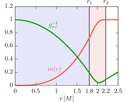
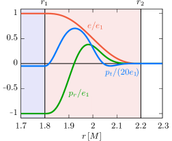
Figure 3: Metric functions (left panel) and fluid pressures and energy density (right panel) for a representative anisotropic-pressure gravastar with a mass $M$. In analogy with Fig. 1, the blue (red) shading refers to the de-Sitter interior (matter shell); the inner radius is $r_{1}=1.8\,M$ and the outer radius is $r_{2}=2.2\,M$. The tangential pressure is scaled by a factor of $1/20$ for better visualisation, but provides the dominant contribution in the Einstein equations.

Figure 3 provides a useful example of the radial behaviour of the metric quantities (left panel) and of the fluid quantities (right panel) for a representative anisotropic-pressure gravastar with a mass $M$. The inner radius is $r_{1}=1.8\,M$ and the outer radius is $r_{2}=2.2\,M$; note that the tangential pressure is scaled by a factor of $1/20$ for better visualisation, but effectively provides the dominant contribution in the Einstein equations.

3.3 Space of solutions of anisotropic-pressure gravastars

Also when constructing gravastars with an anisotropic pressure, the space of possible solutions is limited in terms of the compactness $\mathcal{C}:=M/r_{2}$ and shell thickness $\delta:=r_{2}-r_{1}$. Fig. 4 shows this behaviour, and the corresponding data has been obtained by following the same approach employed for the isotropic thin-shell gravastar, where the solid green line marks the edge of the allowed solutions, denoting with $\delta_{\rm crit}\simeq 2.4740\,M$ the critical shell thickness with a corresponding critical compactness of $\mathcal{C}_{\rm crit}\simeq 0.4042$, dividing the edge again into a restricted branch with $\delta<\delta_{\rm crit}$ and an unrestricted branch with $\delta>\delta_{\rm crit}$ . The existence of the restricted branch is essentially the result of our choice for the energy-density function (25) and of the ability to prevent the formation of an event horizon by satisfying the condition (34) [we recall that different choices of $e(r)$ automatically map into different choices of the function $m(r$) via the definition (22)]. Indeed, apart from the two-branches case considered here, other and suitable choices of the function $e(r)$ would lead to either a single unrestricted branch following the condition (17) or to a single restricted branch. It is possible to examine this behaviour by looking at the limit of $r_{1}\to 0$, inspecting the energy density, mass function and condition (34), noting whether the condition is fulfilled for all compactnesses or not. Solutions cannot go beyond the hyperbole (17), as that would imply negative $r_{1}$; also in this case, a red asterisk marks the isotropic-pressure (thin-shell) gravastar. A more detailed discussion of the radial structure of the gravastar solutions along the edge of equilibria can be found in Appendix 6.

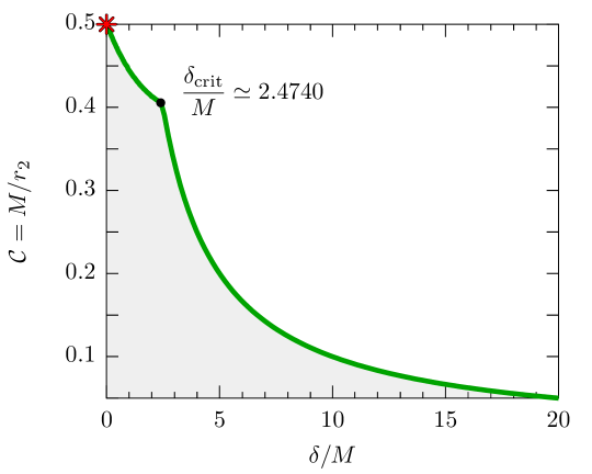
Figure 4: The same as in Fig. 2 but for an anisotropic-pressure gravastar. Shown with a red asterisk is the isotropic-pressure (thin-shell) gravastar solution.

4 Nestars

Having recalled the construction of anisotropic-pressure gravastars, we can now proceed with the same basic formalism to develop instead a multi-layered compact object composed of two nested gravastars, that is, a “nestar”. In practice, we now split the spherically symmetric and static spacetime into the following five regions:

I.     de-Sitter shell $$r\in\left[0,r_{1}\right)\,, p=-e_{1}\,,$$ (35)

II.   matter shell $$r\in\left[r_{1},r_{2}\right]\,, p=p(e)\,,$$ (36)

III.  de-Sitter-shell $$r\in\left(r_{2},r_{3}\right)\,, p=-e_{3}\,,$$ (37)

IV.  matter shell $$r\in\left[r_{3},r_{4}\right]\,, p=p(e)\,,$$ (38)

V.   vacuum exterior $$r\in\left(r_{4},\infty\right)\,, p=e=0\,.\hskip 28.45274pt$$ (39)

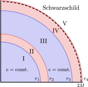
Figure 5: Illustrative representation of a nestar. Note the addition of regions III and IV, which represent a replica of regions I and II, before the spacetime is smoothly joined with the Schwarzschild portion V.

Obviously, this construction would not work if one had in mind the nesting of two stratified ordinary stars, as the addition of the second star would completely change any hydrostatic equilibrium (the new shells would just increase the gravitational field as gravity is attractive for both). However, as discussed in the introduction, it is reasonable to expect that, in the case of gravastars, this construction could lead to a new equilibrium as each of the two gravastar can be considered in near hydrostatic equilibrium, so that nesting them into each other should be possible. Figure 5 provides an illustrative representation of a nestar, where the addition of regions III and IV should be noted, which represent a replica of regions I and II, before the spacetime is smoothly joined with the Schwarzschild portion V. Finally, as we will see below, this intuition of nesting gravastars as in a “matryoshka doll” – a collection of wooden dolls diminishing in size and nested within each other – is correct in the case of anisotropic-pressure (thick-shell) gravastars and incorrect in the case of isotropic-pressure (thin-shell) gravastars.

4.1 No-go theorem for an isotropic-pressure (thin-shell) nestar

We start by proceeding in analogy with what done in the case of the construction of the gravastar layered spacetime and split the nestar spacetime into the following layers [cf. Eqs. (8) – (10)]

I.   1st de-Sitter shell: $$\begin{cases}\begin{aligned} f(r)&=C(1-H_{0}^{2}r^{2})\,,\\[10.00002pt] h(r)&=1-H_{0}^{2}r^{2}\,,\end{aligned}\end{cases}$$ (40)

II.  1st matter-shell: $$\begin{cases}\begin{aligned} f(r)&={w_{1}}\,f(r_{1})/{w(r)}\,,\\[10.00002pt] h(r)&=\epsilon\,{[1+w(r)]^{2}}/{w(r)}\,,\end{aligned}\end{cases}$$ (41)

III. 2nd de-Sitter shell: $$\begin{cases}\begin{aligned} f(r)&=D(1-\tilde{H}_{0}^{2}r^{2})\,,\\[10.00002pt] h(r)&=1-\tilde{H}_{0}^{2}r^{2}\,,\end{aligned}\end{cases}$$ (42)

IV. 2nd matter shell: $$\begin{cases}\begin{aligned} f(r)&={w_{3}}\,f(r_{3})/{w(r)}\,,\\[10.00002pt] h(r)&=\gamma\,{[1+w(r)]^{2}}/{w(r)}\,,\end{aligned}\end{cases}$$ (43)

V.   exterior: $$\begin{cases}\begin{aligned} f(r)&=1-{2M}/{r}\,,\\[10.00002pt] h(r)&=1-{2M}/{r}\,,\end{aligned}\end{cases}$$ (44)

where $\epsilon,\gamma,C,D,H_{0},\tilde{H}_{0}$, and $M$ are constants to be determined via continuity conditions on the metric functions, while $r_{i}$ and $w_{i}:=w(r_{i})$, with $i=1,...,4$, are free parameters.

As dictated by the thin-shell approximation, the metric functions $h(r)$ in the matter-shell regions II and IV have to go to zero in this limit, namely,

$$h_{\rm II}(r)\to 0\,,\qquad h_{\rm IV}(r)\to 0\,.$$ (45)

However, since we impose continuity on all metric functions, the ones in the second de-Sitter shell and between the thin matter shells, have to approach zero at their outer edges, i.e.,

$$h_{\rm III}(r_{2})=1-\tilde{H}_{0}^{2}r_{2}^{2}\to 0\,,\qquad h_{\rm III}(r_{3})=1-\tilde{H}_{0}^{2}r_{3}^{2}\to 0\,,$$ (46)

or, equivalently,

$$\tilde{H}_{0}^{2}\to\frac{1}{r_{2}^{2}}\,,\qquad\tilde{H}_{0}^{2}\to\frac{1}{r_{3}^{2}}\,.$$ (47)

Bearing in mind that $\tilde{H}_{0}^{2}$ is the same constant in region III, which is a de-Sitter shell, means that fulfilling the condition (47) is possible only if

$$r_{2}\to r_{3}\,,$$ (48)

that is, if the second de-Sitter shell (or region III), has zero radial extent. However, removing such a shell implies that the two matter shells II and IV are now adjacent and hence they are effectively a single shell ranging from $r_{2}$ to $r_{4}$, that is, a standard gravastar. Stated differently, it is not possible to build a meaningful nestar solution so long as one employs an isotropic pressure, as in the original Mazur-Mottola thin-shell gravastar. In turn, this implies that nestars will have to be built with anisotropic pressures, as we illustrate next.

4.2 Anisotropic-pressure nestar

Having shown that an isotropic-pressure (thin-shell) nestar necessarily coincides with an isotropic-pressure (thin-shell) gravastar, we resort to the same expedient adopted for gravastars and introduce an anisotropic pressure. In essence, we use the anisotropic-pressure gravastar from Sec. 3 and use Eqs. (18)–(22), with modified continuity conditions (23) and (24) to meet the requirements of a nestar

$$\begin{aligned} \text{II.\leavevmode\nobreak\ 1st\leavevmode\nobreak\ matter\leavevmode\nobreak\ shell:\leavevmode\nobreak\ }&\begin{cases}\begin{aligned} e(0)&=e(r_{1})=e_{1}\,,\\[10.00002pt] e^{\prime}(r_{1})&=e^{\prime}(r_{2})=0\,,\\[10.00002pt] e^{\prime\prime}(r_{1})&=e^{\prime\prime}(r_{2})=0\,,\\[10.00002pt] e(r_{2})&=e_{3}\,,\end{aligned}\end{cases}\hskip 10.00002pt\\[10.00002pt] \text{IV.\leavevmode\nobreak\ 2nd\leavevmode\nobreak\ matter\leavevmode\nobreak\ shell:\leavevmode\nobreak\ }&\begin{cases}\begin{aligned} e(r_{2})&=e(r_{3})=e_{3}\,,\\[10.00002pt] e^{\prime}(r_{3})&=e^{\prime}(r_{4})=0\,,\\[10.00002pt] e^{\prime\prime}(r_{3})&=e^{\prime\prime}(r_{4})=0\,,\\[10.00002pt] e(r_{4})&=0\,.\end{aligned}\end{cases}\end{aligned}$$ (49)

We can satisfy these conditions via the following layered prescription for the energy density

$$e(r)=\left\{\begin{aligned} &e_{1}={\rm const.}&\quad{\rm for}\quad&0\leq r<r_{1}\,,\quad&&\text{:\leavevmode\nobreak\ I.\leavevmode\nobreak\ 1st\leavevmode\nobreak\ de-Sitter\leavevmode\nobreak\ shell}\,,\\ &\sum^{5}_{i=0}a_{i}\,r^{i}&\quad{\rm for}\quad&r_{1}\leq r\leq r_{2}\,,\quad&&\text{:\leavevmode\nobreak\ II.\leavevmode\nobreak\ 1st\leavevmode\nobreak\ matter\leavevmode\nobreak\ shell}\,,\\ &e_{3}={\rm const.}&\quad{\rm for}\quad&r_{2}<r<r_{3}\,,\quad&&\text{:\leavevmode\nobreak\ III.\leavevmode\nobreak\ 2nd\leavevmode\nobreak\ de-Sitter\leavevmode\nobreak\ shell}\,,\\ &\sum^{5}_{i=0}b_{i}\,r^{i}&\quad{\rm for}\quad&r_{3}\leq r\leq r_{4}\,,\quad&&\text{:\leavevmode\nobreak\ IV.\leavevmode\nobreak\ 2nd\leavevmode\nobreak\ matter\leavevmode\nobreak\ shell}\,,\\ &\quad 0&\quad{\rm for}\quad&r_{4}<r\,,\quad&&\text{:\leavevmode\nobreak\ V.\leavevmode\nobreak\ exterior}\,.\end{aligned}\right.$$ (50)

Note that modifications to the EOS in the matter shell are also necessary since Eq. (28) can only connect an adjacent nonzero energy-density de-Sitter shell with an adjacent vacuum exterior, while we here need to connect two nonzero energy-density de-Sitter shells. As a result, a possible option for the EOSs in the regions I-IV is as follows

$$p_{r}(e)=\left\{\begin{aligned} &-e_{1}&\quad{\rm for}\quad&0\leq r<r_{1}\,,\\[5.0pt] &e\Biggl{[}\alpha_{2}-(1+\alpha_{2})\frac{(e-e_{3})^{3}-(e-e_{1})^{3}}{(e_{1}-e_{3})^{3}}\Biggr{]}&\quad{\rm for}\quad&r_{1}\leq r\leq r_{2}\,,\\[5.0pt] &-e_{3}&\quad{\rm for}\quad&r_{2}<r<r_{3}\,,\\[5.0pt] &\left(\frac{e^{2}}{e_{3}}\right)\Biggl{[}\alpha_{4}-(1+\alpha_{4})\left(\frac{e}{e_{3}}\right)^{2}\Biggr{]}&\quad{\rm for}\quad&r_{3}\leq r\leq r_{4}\,,\\[5.0pt] &\quad 0&\quad{\rm for}\quad&r_{4}<r\,,\end{aligned}\right.$$ (51)

where the constants $\alpha_{2}$ and $\alpha_{4}$ are not constrained yet, but play the same role of the constant $\alpha$ in the EOS (28). In particular, we can require that the newly proposed EOS continues to satisfy the following set of conditions [25]

1. it must satisfy at least the less stringent energy conditions, namely, the dominant energy-condition $(e\geq\lvert p_{r}\rvert)$ and the weak energy-condition $(e\geq 0$ and $e+p_{r}\geq 0)$;

2. the corresponding sound speed must always be subliminal;

3. the corresponding sound speed does not have a maximum at $e=0$.

Requiring these conditions to hold yields the parameters

$$\alpha_{2}=\frac{e_{1}^{2}-3e_{1}e_{3}+e_{3}^{2}}{e_{1}^{2}-e_{1}e_{3}+e_{3}^{2}}\,,$$ (52)

$$\alpha_{4}=\frac{3}{4}\Biggl{[}\sqrt[3]{4-2\sqrt{2}}+\sqrt[3]{2(2+\sqrt{2})}\,\Biggr{]}\simeq 2.2135\,.$$ (53)

It is important to underline that within this framework it is not possible to choose $e_{1}=e_{3}$, as all the polynomial coefficients for the energy density in region II would reduce to zero except for the first one, which would be trivially be given by $a_{0}=e_{1}=e_{3}$, thus falling back into the case of an anisotropic-pressure gravastar. To address this issue, we impose an additional condition in region II by requiring that the energy density in the midpoint of region II is proportional to the energy density in region I, so that the polynomial has to cross at least one point and does not reduce to a constant, i.e.,

$$e|_{(r_{1}+r_{2})/2}=(1-\chi)\,e_{1}\,,\qquad{\rm with}\qquad\chi\in(0,1)\,.$$ (54)

We note that because of the additional condition (54), the polynomial description of the energy density becomes of sixth order with an additional polynomial coefficient $a_{6}$. Furthermore, the introduction of the free parameter $\chi\in(0,1)$ is useful not only for two nested gravastars, but also when we will consider $N$ nested gravastars in Sec. 4.4.

Given the generality of the energy density and EOS considered, there is a large freedom in the construction of two nested gravastars and in what follows we consider two specific classes. The first one is reminiscent of a “copy-paste” operation, in that the energy density of regions I and III are set to be the same, namely, $e_{1}=e_{3}$. In this case, because the EOS (51) in region II would have a zero in the denominator, we need to use in such a region the same EOS used for a single gravastar (28), as it is capable of connecting two de-Sitter shells with the same energy density.

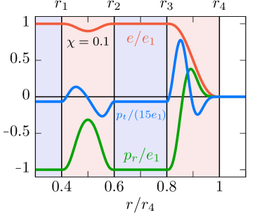
Figure 6: The same as in Fig. 3 but for a representative nestar with a mass $M$, outer radius $r_{4}=5\,M$, and where energy densities in regions I and III are the same, i.e., $e_{1}=e_{3}$ and $\chi=0.1$ from (54). For better visualisation, the tangential pressure is scaled by a factor of $1/15$, while the mass function is scaled by a factor of $100$.

A bit of algebra allows one to deduce that the set of unknown coefficients in the energy-density function for the first matter shell in region II are given by

$$\begin{aligned} a_{6}&=\frac{64\chi\,e_{1}}{(r_{2}-r_{1})^{6}}\,,&\quad a_{5}&=-\frac{192\chi\,e_{1}(r_{1}+r_{2})}{(r_{2}-r_{1})^{6}}\,,\\[10.00002pt] a_{4}&=\frac{192\chi\,e_{1}(r_{1}^{2}+3r_{1}r_{2}+r_{2}^{2})}{(r_{2}-r_{1})^{6}}\,,&\quad a_{3}&=-\frac{64\chi\,e_{1}(r_{1}+r_{2})(r_{1}^{2}+8r_{1}r_{2}+r_{2}^{2})}{(r_{2}-r_{1})^{6}}\,,\\[10.00002pt] a_{2}&=\frac{192\chi\,e_{1}r_{1}r_{2}(r_{1}^{2}+3r_{1}r_{2}+r_{2}^{2})}{(r_{2}-r_{1})^{6}}\,,&a_{1}&=-\frac{192\chi\,e_{1}r_{1}^{2}r_{2}^{2}(r_{1}+r_{2})}{(r_{2}-r_{1})^{6}}\,,\\[10.00002pt] a_{0}&=e_{1}+\frac{64\chi\,e_{1}r_{1}^{3}r_{2}^{3}}{(r_{2}-r_{1})^{6}}\,,\\ \end{aligned}$$

while the coefficients in the energy-density function for the second matter shell in region IV are given by

$$\begin{aligned} b_{5}&=-\frac{6e_{1}}{(r_{4}-r_{3})^{5}}\,,&\qquad\hskip 4.40002ptb_{4}&=\frac{15e_{1}(r_{3}+r_{4})}{(r_{4}-r_{3})^{5}}\,,\\[10.00002pt] b_{3}&=-\frac{10e_{1}(r_{3}^{2}+4r_{3}r_{4}+r_{4}^{2})}{(r_{4}-r_{3})^{5}}\,,&\qquad b_{2}&=\frac{30e_{1}r_{3}r_{4}(r_{3}+r_{4})}{(r_{4}-r_{3})^{5}}\,,\\[10.00002pt] b_{1}&=-\frac{30e_{1}r_{3}^{2}r_{4}^{2}}{(r_{4}-r_{3})^{5}}\,,&\qquad b_{0}&=\frac{e_{1}r_{4}^{3}(10r_{3}^{2}-5r_{3}r_{4}+r_{4}^{2})}{(r_{4}-r_{3})^{5}}\,.\end{aligned}$$

Figure 6 shows a representative solution for the case of two nested gravastars having the same energy density in the de-Sitter shells. In particular, it refers to a nestar with a mass $M$ and outer radius $r_{4}=5\,M$. Note that all the metric functions and fluid variables, as well as their first derivatives, are continuous; the tangential pressure (30) is still the dominant one and scaled by a factor of $1/15$, while the mass function is scaled by a factor of $100$ for better visibility.

Following a similar logic, it is possible to construct equilibrium solutions also for two nested gravastars when the de-Sitter shells have different energy densities $e_{1}\neq e_{3}$. Also in this case, straightforward algebra allows one to deduce that the set of unknown coefficients in the energy-density function for the first matter shell in region II are given by

$$\begin{aligned} a_{5}&=\frac{6(e_{3}-e_{1})}{(r_{2}-r_{1})^{5}}\,,&\,a_{4}&=-\frac{15(e_{3}-e_{1})(r_{1}+r_{2})}{(r_{2}-r_{1})^{5}}\,,\\[10.00002pt] a_{3}&=\frac{10(e_{3}-e_{1})(r_{1}^{2}+4r_{1}r_{2}+r_{2}^{2})}{(r_{2}-r_{1})^{5}}\,,&\,a_{2}&=-\frac{30(e_{3}-e_{1})(r_{1}+r_{2})r_{1}r_{2}}{(r_{2}-r_{1})^{5}}\,,\\[10.00002pt] a_{1}&=\frac{30(e_{3}-e_{1})r_{1}^{2}r_{2}^{2}}{(r_{2}-r_{1})^{5}}\,,&\,a_{0}&=e_{3}-\frac{(e_{3}-e_{1})(10r_{1}^{2}-5r_{1}r_{2}+r_{2}^{2})r_{2}^{3}}{(r_{2}-r_{1})^{5}}\,,\end{aligned}$$

while the coefficients in the energy-density function for the second matter shell in region IV are given by

$$\begin{aligned} b_{5}&=-\frac{6e_{3}}{(r_{4}-r_{3})^{5}}\,,&\qquad\hskip 4.40002ptb_{4}&=\frac{15e_{3}(r_{3}+r_{4})}{(r_{4}-r_{3})^{5}}\,,\\[10.00002pt] b_{3}&=-\frac{10e_{3}(r_{3}^{2}+4r_{3}r_{4}+r_{4}^{2})}{(r_{4}-r_{3})^{5}}\,,&\qquad b_{2}&=\frac{30e_{3}r_{3}r_{4}(r_{3}+r_{4})}{(r_{4}-r_{3})^{5}}\,,\\[10.00002pt] b_{1}&=-\frac{30e_{3}r_{3}^{2}r_{4}^{2}}{(r_{4}-r_{3})^{5}}\,,&\qquad b_{0}&=\frac{e_{3}r_{4}^{3}(10r_{3}^{2}-5r_{3}r_{4}+r_{4}^{2})}{(r_{4}-r_{3})^{5}}\,.\end{aligned}$$

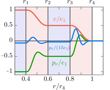
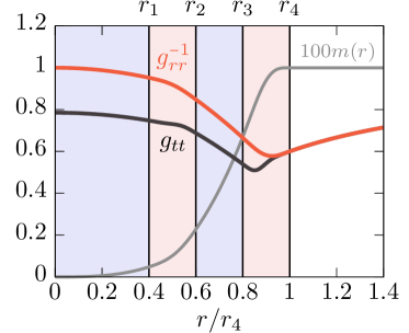
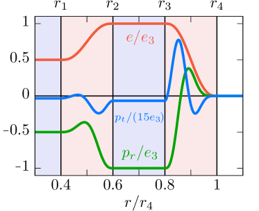
Figure 7: The same as in Fig. 6 but for a representative nestar with different energy densities in the matter shells. The upper row refers to a nestar with decreasing energy densities $e_{1}>e_{3}$, while the lower row to one with increasing energy densities $e_{1}<e_{3}$.

Figure 7 provides the equivalent information as Fig. 6 but for a nestar having de-Sitter shells with decreasing energy density $e_{1}>e_{3}$ (upper row) and an increasing one $e_{1}<e_{3}$ (lower row). Note that also in these cases, all the metric functions and fluid variables, as well as their first derivatives, are continuous. Similarly, the tangential pressure still provides the dominant contribution to the equilibrium.

4.3 Space of solutions of anisotropic-pressure nestars

The systematic analysis we have carried out for the anisotropic-pressure gravastar can be extended in the case of a nestar, where all possible equilibrium configurations need to respect the no-horizon condition (34). The main difference here is that the space of solutions will obviously be larger and can be characterised in terms of the thickness of the two matter shells, namely, $\delta_{2}:=r_{2}-r_{1}$ and $\delta_{4}:=r_{4}-r_{3}$, and of the overall compactness $\mathcal{C}:=M/r_{4}$.

Figure 8 shows the space of all such possible solutions of the nestar compactness $\mathcal{C}$, when expressed in terms of two matter-shell thicknesses $\delta_{2}$ and $\delta_{4}$. As for gravastars, here the two-dimensional surface marks the limit above which no nestar solution can be found because the no-horizon condition does not hold anymore or the matter shells already encompass the whole nestar. Note that the overall behaviour is similar but also distinct from that already encountered for the thin-shell gravastar in Fig. 2 and for the anisotropic-pressure gravastar in Fig. 4.

In particular along the surface, for specific combinations of $\delta_{2}$ and $\delta_{4}$, there exists a critical compactness $\mathcal{C}_{\rm crit}$ distinguishing the restricted and unrestricted branch of the space of solutions and this is marked with a white solid line on the limiting surface in Fig. 8. Solutions approaching the surface beneath the critical line can be described with a generalisation of the hyperbolic condition for two matter shells

$$\mathcal{C}\,\frac{\delta_{2}+\delta_{4}}{M}=\frac{\delta_{2}+\delta_{4}}{r_{4}}\to 1\qquad\Rightarrow\qquad\delta_{2}+\delta_{4}\to r_{4}\,,$$ (59)

which can be interpreted as the case in which both matter shells encompass the whole nestar, thus in full analogy with what we have seen in the case of the gravastar, where the hyperbolic condition (17) also referred to the situation in which the matter shell encompassed the whole object. Therefore, the surface below the critical line marks the unrestricted solutions, while the red asterisk helps locate the position in the space of solutions of the isotropic-pressure (thin-shell) gravastar.

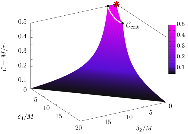
Figure 8: Space of possible solutions for nestars represented in terms of the nestar compactness $\mathcal{C}:=M/r_{4}$ and of the thicknesses of the matter shells $\delta_{2}:=r_{2}-r_{1}$, $\delta_{4}:=r_{4}-r_{3}$. The coloured surface marks the limit of the space of solutions beyond which an event horizon appears or $r_{1}<0$, while the white line shows the position of the critical compactness $\mathcal{C}_{\rm crit}$ dividing the two branches already encountered for a single-shell gravastar. Shown with a red asterisk is the isotropic-pressure (thin-shell) gravastar solution.

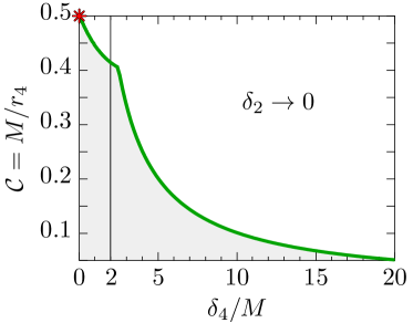
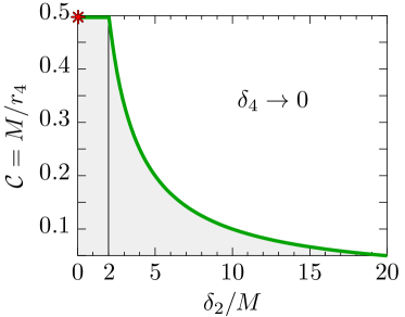
Figure 9: Sections at constant values of the inner matter shell thickness ($\delta_{2}\to 0$, left panel) or at constant outer matter shell thickness ($\delta_{4}\to 0$, right panel) for the compactness of the admitted solutions for nestars. The left panel coincides with the limit of a standard anisotropic-pressure gravastar, while the right panel reports the disappearance of the restricted branch and thus yields solutions approaching a compactness of $\mathcal{C}\to(1/2)^{-}$ whilst being comprised of essentially only matter. Shown with a red asterisk is the isotropic-pressure (thin-shell) gravastar solution.

Shown instead in Fig. 9 are two sections of the space of solutions for the compactness of the nestar at constant values of the inner-shell thickness ($\delta_{2}\to 0$, left panel) or at constant outer-shell thickness ($\delta_{4}\to 0$, right panel) for the compactness. Starting from the left panel, it is easy to realise that this limit corresponds essentially to a standard anisotropic-pressure gravastar [cf. Fig. 4]; indeed, $\delta_{4}$ exhibits a critical thickness which is the same encountered for an anisotropic-pressure gravastar, i.e., $\delta_{\rm crit}:=(\delta_{2,{\rm crit}},\delta_{4,{\rm crit}})\simeq(0,2.4740\,M)$ [also in this case, we can mark a critical compactness $\mathcal{C}_{\rm crit}\simeq 0.4042$]. Far more interesting is the space of solutions shown in the right panel (i.e., for $\delta_{4}\to 0$) for in this case the restricted branch disappears, and where nestar solutions approaching the green line have a particularly interesting structure. More specifically, the outer de-Sitter and the outer matter shell (regions III and IV) are of infinitesimal size ($r_{2}\to r_{3}\to r_{4}>2\,M$) because the green line corresponds to $\mathcal{C}\delta_{2}/M\to 1\Rightarrow\delta_{2}\to r_{4}$. As a result, the inner de-Sitter shell (region I) is also infinitesimal ($r_{1}\to 0$) and the inner matter shell (region II) fills the whole nestar. In this way, the critical thickness is moved to $\delta_{\rm crit}\to(2\,M^{+},0)$ and the critical compactness to $\mathcal{C}_{\rm crit}\to(1/2)^{-}$; clearly, the condition $r_{2}\to r_{3}\to r_{4}\to 2\,M^{+}$ is met when the compactness is the maximal allowed, i.e., $\mathcal{C}\to(1/2)^{-}$. This is a particularly interesting configuration, where the compactness is maximal but the interior of the compact object is essentially all filled of matter. This is to be contrasted with the isotropic-pressure, thin-shell gravastar model that has $r_{1}\to r_{2}\to 2M$ and hence where the compact object is essentially all filled by the de-Sitter portion. A more detailed discussion of the radial structure of the nestar solutions along the two sections $\delta_{2}\to 0$ and $\delta_{4}\to 0$ can be found in Appendix 6.

As a concluding remark, we note that what makes the nestar solution with $r_{1}\to 0$, $r_{2}\to r_{3}\to r_{4}\to 2\,M^{+}$, and $\mathcal{C}\to(1/2)^{-}$ particularly fascinating is that it effectively replaces a Schwarzschild black-hole with a solution that has essentially the same compactness, but where the singularity is replaced by a regular point-like de-Sitter interior and where the null surface is replaced by an ordinary time-like surface with two infinitesimal shells (de-Sitter and matter), while the rest is filled with matter satisfying the weak and dominant energy conditions. Hence, when going back to the issue of the genesis of these speculative objects, the nestar in question could be considered as a more plausible endpoint of a gravitational collapse since the appearance of a singularity would be replaced by the appearance of only a point-like de-Sitter mini-universe and not a whole de-Sitter interior.

4.4 Anisotropic-pressure multi-layer nestar

We conclude our discussion by generalising many of the concepts and the formalism introduced so far in the case of two nested gravastars to the case of $K$ nested gravastars, where $K$ is an arbitrary integer. Once again, intuition serves as a useful guide to understand why a construction with $K$ nested gravastars should be reasonable if an equilibrium solution can be found for two. Let us recall that because of the balanced interplay between the expanding interior and the contracting shell, each gravastar is essentially in equilibrium, so that the operation of nesting gravastars into each other will not radically change such an equilibrium. Exactly for this reason, it is reasonable to expect that the same logic should apply also when the nesting is done for two gravastars or for $K$, with $K$ arbitrary.

In practice, we proceed exactly as done in the case of two nested gravastars in Sec. 4 [see Eqs. (35)–(39)] , and split now the spacetime not into five regions but into $2K+1$ regions, $K$ of which are filled by de-Sitter shells with constant energy densities and negative pressures, $K$ by matter shells with however complicated EOSs, and the $2K+1$-th region is that with a vacuum and hence described by the Schwarzschild solution. In essence, we describe the nesting of $K$ gravastars to produce a $2K$-shells nestar using the following scheme

de-Sitter shells $$r\in\left(r_{2k-2},r_{2k-1}\right)\,,$$ (60)

matter shells $$r\in\left[r_{2k-1},r_{2k}\right]\,,$$ (61)

exterior $$r\in\left(r_{2K},\infty\right)\,,$$

$$\hskip 85.35826ptk\in\mathbb{N}\,,\quad k\in[1,K]\,,$$

where the radii $r_{2k-1}$ and $r_{2k}$ are free parameters except for the centre, which obviously needs to be at $r_{0}=0$; the edge of the outermost shell, and thus of the nestar, is at $r_{2K}$.

Recalling that the (odd) interior de-Sitter shells are of constant energy density while the (even) matter-shell regions have energy densities expressed in terms of polynomial functions, the complete energy-density function can be written in a compact manner as

$$e(r)=\left\{\begin{aligned} &e_{2k-1}={\rm const.}&\quad{\rm for}\quad&r\in\left(r_{2k-2},r_{2k-1}\right)\,,\\ &E_{2k}(r)&\quad{\rm for}\quad&r\in\left[r_{2k-1},r_{2k}\right]\,,\\ &e_{2K+1}=0&\quad{\rm for}\quad&r\in\left(r_{2K},\infty\right)\,,\end{aligned}\right.$$ (63)

$$k\in\mathbb{N}\,,\quad k\in[1,K]\,,$$

where $e_{2k-1}$ are free parameters. Depending on whether the energy density has to connect two de-Sitter shells with the same energy density or two different ones, one will either choose a 6th-order or a 5th-order polynomial ($e_{2K+1}=0$ so that the last shell is 5th-order), namely

$$E_{2k}(r)=\left\{\begin{aligned} &\sum^{6}_{i=0}a_{i,2k}\,r^{i}\,,&\quad&e_{2k-1}=e_{2k+1}\,,\\ &\sum^{5}_{i=0}\tilde{a}_{i,2k}\,r^{i}\,,&\quad&e_{2k-1}\neq e_{2k+1}\,,\end{aligned}\right.$$ (64)

$$\hskip 2.56064ptk\in\mathbb{N}\,,\quad k\in[1,K]\,;$$

the full expressions for the coefficients ${a}_{i,2k}$ and $\tilde{a}_{i,2k}$ as a function of the various radii and energy densities can be found in Appendix 6.

Similarly, the radial pressure can be expressed as

$$p_{r}(e)=\left\{\begin{aligned} &-e_{2k-1}&\quad{\rm for}\quad&r\in\left(r_{2k-2},r_{2k-1}\right)\,,\\ &P_{2k}(e)&\quad{\rm for}\quad&r\in\left[r_{2k-1},r_{2k}\right]\,,\\ &\quad 0&\quad{\rm for}\quad&r\in\left(r_{2K},\infty\right)\,,\end{aligned}\right.$$ (65)

$$k\in\mathbb{N}\,,\quad k\in[1,K]\,,$$

where the de-Sitter shells have a simple $p=-e$ EOS in the spirit of a de-Sitter spacetime. The EOSs for the matter-shell regions are instead computed depending on whether the energy densities are the same or different across the adjacent de-Sitter shell regions

$$P_{2k}(e)=\left\{\begin{aligned} &\frac{E_{2k}^{2}(r)}{e_{2k-1}}\Biggl{[}\alpha_{2k}-(1+\alpha_{2k})\left(\frac{E_{2k}(r)}{e_{2k-1}}\right)^{2}\Biggr{]}\,,\hskip 58.6126pte_{2k-1}=e_{2k+1}\,,\\[6.99997pt] &E_{2k}(r)\Biggl{[}\alpha_{2k}-(1+\alpha_{2k})\frac{(E_{2k}(r)-e_{2k+1})^{3}-(E_{2k}(r)-e_{2k-1})^{3}}{(e_{2k-1}-e_{2k+1})^{3}}\Biggr{]}\,,\\[5.0pt] &\hskip 227.62204pte_{2k-1}\neq e_{2k+1}\,,\end{aligned}\right.$$ (66)

$$k\in\mathbb{N}\,,\quad k\in[1,K]\,,$$

modifying the definitions of (52) for a $2K$-layers nestar

$$\alpha_{2k}=\left\{\begin{aligned} &\frac{3}{4}\Biggl{[}\sqrt[3]{4-2\sqrt{2}}+\sqrt[3]{2(2+\sqrt{2})}\,\Biggr{]}\simeq 2.2135\,,&e_{2k-1}=e_{2k+1}\,,\\[5.0pt] &\frac{e_{2k-1}^{2}-3e_{2k-1}e_{2k+1}+e_{2k+1}^{2}}{e_{2k-1}^{2}-e_{2k-1}e_{2k+1}+e_{2k+1}^{2}}\,,&e_{2k-1}\neq e_{2k+1}\,,\end{aligned}\right.$$ (67)

$$\hskip 35.00005ptk\in\mathbb{N}\,,\quad k\in[1,K]\,.$$

Finally, the tangential pressure can be computed using Eq. (30), so that, after choosing the radii $r_{2k-1}$, $r_{2k}$ and the de-Sitter energy densities $e_{2k-1}$, it is possible to build a $2K$-layers nestar with Eqs.  (63)–(67) and the polynomial coefficients that are reported in Appendix 6.

We conclude this section and this work by pushing even further the level of speculation. Given that: (i) a nestar with an arbitrarily large number of layers is possible to construct; (ii) that the maximum compactness that is possible to reach is smaller but arbitrarily close to that of a Schwarzschild black hole; (iii) the volume fraction of the nestar that satisfies the weak and dominant energy conditions can be taken arbitrarily close to one, a multi-layer nestar could represent an interesting alternative to a black hole solution with the advantage of being everywhere regular and nonvacuum.

5 Conclusion

More than 20 years ago, Mazur and Mottola proposed the isotropic (thin-shell) gravastar model [1, 6], which has since then attracted attention and triggered considerable related work. More importantly, the gravastar model has suggested a new way of thinking about compact objects and whether alternatives to black holes without an event horizon can be envisaged as the final point of gravitational collapse. Twenty years later, and while many of the aspects of these objects are now well understood, a number of issues remain unsolved about their dynamical formation or the corresponding observability [22, 19, 23, 26].

We have here revisited the gravastar model and raised the bar of speculation by considering new solutions that are inspired by the original model but also offer surprising new features. In particular, we have shown that when using anisotropic pressure it is possible to nest two gravastars into each other and obtain a new and rich class of solutions of the Einstein equations. Indeed, thanks to the fact that each gravastar essentially behaves as a distinct self-gravitating equilibrium configuration, a very large space of parameters exists for nested gravastars having an anisotropic pressure support. In this space of solutions, one is particularly interesting since it replaces a Schwarzschild black-hole with a solution that has essentially the same compactness, but where the singularity is replaced by a regular point-like de-Sitter interior and where the null surface is replaced by an ordinary time-like surface with two infinitesimal shells (de-Sitter and matter), while the rest is filled with matter satisfying the weak and dominant energy conditions. Finally, we have shown that the nested two-gravastar solutions can be extended to an arbitrarily large number of elements, with a prescription that can be easily specified in terms of recursive relations.

Although these equilibria are admittedly on the exotic side of astrophysical compact objects, it is interesting to note that more than 100 years after the introduction of general relativity, new solutions can be still found in one of the simplest spacetimes: spherically symmetric, static, and not in vacuum. The results presented here can be further explored in a number of different directions, which include: the study of different EOSs, the stability of these solutions against perturbations and the corresponding quasi-normal modes, the existence of stable and unstable circular photon orbits (see [27] for a comprehensive discussion), the extension to rotating configurations (the different shells can have the same or different angular velocities) and their stability [28], and, of course, the exploration of similar equilibria in other theories of gravity.

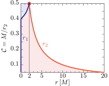
Figure 10: Radial structure of anisotropic-pressure gravastars on the outer edge of the space of possible solutions (i.e., along the green line in Fig. 4). Shown with a red asterisk is the isotropic-pressure (thin-shell) gravastar solution.

6 Appendix

Radial structure of anisotropic-pressure gravastars and nestars

As an example of the complex radial structure of anisotropic-pressure gravastars, we report in Fig. 10 the values of the radii $r_{1}$ and $r_{2}$ as a function of the compactness $\mathcal{C}=M/r_{2}$ for a sequence of gravastars on the outer edge of the space of possible solutions (i.e., along the green line in Fig. 4). Note how for compactnesses smaller than the critical compactness $\mathcal{C}_{\rm crit}\simeq 0.4042$, the solutions are those of the unrestricted branch and hence with an infinitesimal de-Sitter interior ($r_{1}\to 0$) and a matter shell that fills the whole gravastar. However, for compactnesses larger than the critical one, the space of solutions jumps to the restricted branch and the de-Sitter interior expands. When $\mathcal{C}\to(1/2)^{-}$, the matter shell shrinks to an infinitesimal thickness ($r_{1}\to 2\,M^{-}$ and $r_{2}\to 2\,M^{+}$) and the de-Sitter interior tends to fill the entire gravastar.

Similarly, we show in Fig. 11 the values of the radii $r_{1},r_{2},r_{3}$, and $r_{4}$ for a sequence of $K=2$ nestars on the outer edge of the space of possible solutions. In particular, the left panel refers to a section at zero value of the inner matter shell thickness ($\delta_{2}\to 0$), while the right panel to a zero outer matter shell thickness ($\delta_{4}\to 0$). In other words, the left and right panels show respectively the radial structure of the nestars along the green lines in the left and right panels of Fig. 9. Note that the left panel of Fig. 11 is very similar to Fig. 10, with the only difference that now regions I, II and III of the spacetime have infinitesimal thickness ($r_{1}\to r_{2}\to r_{3}\to 0$); in this respect, these nestars are effectively equivalent to gravastars with anisotropic pressure.

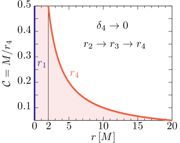
Figure 11: Radial structure for a sequence of $K=2$ nestars on the outer edge of the space of possible solutions, i.e., along the green lines in the left and right panels of Fig. 9. The left panel refers to a section at constant value of the inner-shell thickness ($\delta_{2}\to 0$), while the right panel to a constant outer-shell thickness ($\delta_{4}\to 0$). Shown with a red asterisk is the isotropic-pressure (thin-shell) gravastar solution.

On the other hand, the right panel highlights a rather different radial structure. As already anticipated in the Sec. 4.3, in this case, all solutions are on the unrestricted branch, so that the outer de-Sitter and the outer matter shells (regions III and IV) are of infinitesimal size ($r_{2}\to r_{3}\to r_{4}>2\,M$), because the green line in the right panel of Fig. 9 corresponds to $\mathcal{C}\delta_{2}/M\to 1\Rightarrow\delta_{2}\to r_{4}$. As a result, the inner de-Sitter shell (region I) is also infinitesimal ($r_{1}\to 0$) and the inner matter shell (region II) fills the whole nestar. In this way, the critical thickness is moved to $\delta_{\rm crit}:=(\delta_{2,{\rm crit}},\delta_{4,{\rm crit}})\to(2\,M^{+},0)$ and the critical compactness to $\mathcal{C}_{\rm crit}\to(1/2)^{-}$; clearly, the radii must be such that $r_{2}\to r_{3}\to r_{4}\to 2\,M^{+}$ when the compactness reached is the maximum allowed, i.e., $\mathcal{C}\to(1/2)^{-}$. As mentioned in the main text, this is a particularly interesting configuration, where the compactness is maximal but the interior of the compact object is essentially all filled of matter.

Finally, Fig. 12 provides some representative examples of the radial structure for a sequence of $K=2$ nestars along $\mathcal{C}={\rm const.}$ lines in the $\delta_{4}\to 0$ section of Fig. 9 with $r_{3}\to r_{4}$. In particular, setting $r_{1}=\psi(1-\delta_{2}/r_{4})$ and $r_{2}=r_{1}+\delta_{2}$, the different cases show examples where each de-Sitter shell takes up different fractions of the available space, namely with $\psi=1/4$ in the left panel, $\psi=1/2$ in the middle panel and $\psi=3/4$ in the right panel. Note that the first matter shell, shown with a red shading, can be placed arbitrarily inside the nestar and does not necessarily have to follow the radial structure suggested here. Particularly interesting are the cases when $\mathcal{C}\to(1/2)^{-}$, $\delta_{2}\to 0$ and $\delta_{4}\to 0$, which essentially correspond to the isotropic-pressure (thin-shell) gravastar (see also left panel of Fig. 11).

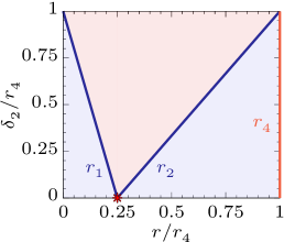
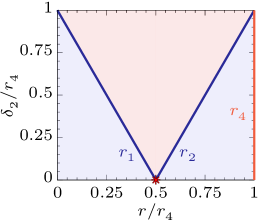
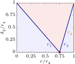
Figure 12: Examples of the radial structure for a sequence of $K=2$ nestars along $\mathcal{C}={\rm const.}$ lines in the $\delta_{4}\to 0$ section of Fig. 9 with $r_{3}\to r_{4}$. Shown are different cases, where each de-Sitter shell takes up different fractions of the available space, namely $r_{1}=\psi(1-\delta_{2}/r_{4})$ and $r_{2}=r_{1}+\delta_{2}$, with $\psi=1/4$ in the left panel, $\psi=1/2$ in the middle panel and $\psi=3/4$ in the right panel. Note that the first matter shell, shown with a red shading above, can be placed arbitrarily inside the nestar and does not necessarily have to follow the radial structure suggested here. Interestingly, when $\mathcal{C}\to(1/2)^{-}$, $\delta_{2}\to 0$ and $\delta_{4}\to 0$, the solutions correspond to the isotropic-pressure (thin-shell) gravastar (see also left panel of Fig. 11), which is marked with a red asterisk.

N-layer nestar coefficients

We here report the polynomial coefficients needed for the energy-density of an anisotropic-pressure nestar with $2K$ shells. As done for the simpler nestar with four shells, we need to distinguish the matter shells regions adjacent to de-Sitter shells having the same energy density from those where the energy densities are different. In the first case, i.e., for $e_{2k-1}=e_{2k+1}$, the coefficients are found to be given by the following recursive relations

$$\begin{aligned} a_{6,2k}&=\frac{64\,\chi_{2k}\,e_{2k-1}}{(r_{2k}-r_{2k-1})^{6}}\,,\\[10.00002pt] a_{5,2k}&=-\frac{192\,\chi_{2k}\,e_{2k-1}(r_{2k-1}+r_{2k})}{(r_{2k}-r_{2k-1})^{6}}\,,\\[10.00002pt] a_{4,2k}&=\frac{192\,\chi_{2k}\,e_{2k-1}(r_{2k-1}^{2}+3r_{2k-1}r_{2k}+r_{2k}^{2})}{(r_{2k}-r_{2k-1})^{6}}\,,\\[10.00002pt] a_{3,2k}&=-\frac{64\,\chi_{2k}\,e_{2k-1}(r_{2k-1}+r_{2k})(r_{2k-1}^{2}+8r_{2k-1}r_{2k}+r_{2k}^{2})}{(r_{2k}-r_{2k-1})^{6}}\,,\\[10.00002pt] a_{2,2k}&=\frac{192\,\chi_{2k}\,e_{2k-1}\,r_{2k-1}\,r_{2k}\,(r_{2k-1}^{2}+3r_{2k-1}r_{2k}+r_{2k}^{2})}{(r_{2k}-r_{2k-1})^{6}}\,,\\[10.00002pt] a_{1,2k}&=-\frac{192\,\chi_{2k}\,e_{2k-1}\,r_{2k-1}^{2}\,r_{2k}^{2}\,(r_{2k-1}+r_{2k})}{(r_{2k}-r_{2k-1})^{6}}\,,\\[10.00002pt] a_{0,2k}&=e_{2k-1}+\frac{64\,\chi_{2k}\,e_{2k-1}\,r_{2k-1}^{3}\,r_{2k}^{3}}{(r_{2k}-r_{2k-1})^{6}}\,.\\ \end{aligned}$$ (68)

$$k\in\mathbb{N}\,,\quad k\in[1,K]\,.$$

On the other hand, in the second case, i.e., for $e_{2k-1}\neq e_{2k+1}$, the coefficients are given by the recursive relations

$$\begin{aligned} \tilde{a}_{5,2k}&=\frac{6(e_{2k+1}-e_{2k-1})}{(r_{2k}-r_{2k-1})^{5}}\,,\\[10.00002pt] \tilde{a}_{4,2k}&=-\frac{15(e_{2k+1}-e_{2k-1})(r_{2k-1}+r_{2k})}{(r_{2k}-r_{2k-1})^{5}}\,,\\[10.00002pt] \tilde{a}_{3,2k}&=\frac{10(e_{2k+1}-e_{2k-1})(r_{2k-1}^{2}+4r_{2k-1}r_{2k}+r_{2k}^{2})}{(r_{2k}-r_{2k-1})^{5}}\,,\\[10.00002pt] \tilde{a}_{2,2k}&=-\frac{30(e_{2k+1}-e_{2k-1})(r_{2k-1}+r_{2k})r_{2k-1}r_{2k}}{(r_{2k}-r_{2k-1})^{5}}\,,\\[10.00002pt] \tilde{a}_{1,2k}&=\frac{30(e_{2k+1}-e_{2k-1})r_{2k-1}^{2}r_{2k}^{2}}{(r_{2k}-r_{2k-1})^{5}}\,,\\[10.00002pt] \tilde{a}_{0,2k}&=e_{2k+1}-\frac{(e_{2k+1}-e_{2k-1})(10r_{2k-1}^{2}-5r_{2k-1}r_{2k}+r_{2k}^{2})r_{2k}^{3}}{(r_{2k}-r_{2k-1})^{5}}\,,\\ \end{aligned}$$ (69)

$$k\in\mathbb{N}\,,\quad k\in[1,K]\,.$$

References

References

- [1] P. O. Mazur and E. Mottola, Gravitational Condensate Stars: An Alternative to Black Holes, arXiv e-prints, (2001), pp. gr–qc/0109035.
- [2] B. P. Abbott et al., Properties of the Binary Black Hole Merger GW150914, Phys. Rev. Lett., 116 (2016), p. 241102.
- [3] K. Akiyama and et al., First M87 Event Horizon Telescope Results. I. The Shadow of the Supermassive Black Hole, Astrophys. J. Lett., 875 (2019), p. L1.
- [4] , First Sagittarius A* Event Horizon Telescope Results. I. The Shadow of the Supermassive Black Hole in the Center of the Milky Way, Astrophys. J. Lett., 930 (2022), p. L12.
- [5] V. Cardoso and P. Pani, Testing the nature of dark compact objects: a status report, Living Reviews in Relativity, 22 (2019), p. 4.
- [6] P. O. Mazur and E. Mottola, Gravitational vacuum condensate stars, Proceedings of the National Academy of Science, 101 (2004), pp. 9545–9550.
- [7] K. Schwarzschild, Über das Gravitationsfeld eines Massenpunktes nach der Einsteinchen Theorie, Sitzungsber. Dtsch. Akad. Wiss. Berlin, Kl. Math. Phys. Tech., 1 (1916), pp. 189–196.
- [8] L. Rezzolla and O. Zanotti, Relativistic Hydrodynamics, Oxford University Press, Oxford, UK, 2013.
- [9] A. D. Sakharov, The Initial Stage of an Expanding Universe and the Appearance of a Nonuniform Distribution of Matter, Soviet Journal of Experimental and Theoretical Physics, 22 (1966), p. 241.
- [10] E. B. Gliner, Algebraic Properties of the Energy-momentum Tensor and Vacuum-like States o+ Matter, Soviet Journal of Experimental and Theoretical Physics, 22 (1966), p. 378.
- [11] W. de Sitter, Einstein’s theory of gravitation and its astronomical consequences, Third Paper, Mon. Not. Roy. Astron. Soc., 78 (1917), pp. 3–28.
- [12] C. B. M. H. Chirenti and L. Rezzolla, How to tell a gravastar from a black hole, Class. Quantum Grav., 24 (2007), pp. 4191–4206.
- [13] E. Mottola, Gravitational Vacuum Condensate Stars, (2023).
- [14] I. Dymnikova, Vacuum nonsingular black hole, General Relativity and Gravitation, 24 (1992), pp. 235–242.
- [15] I. Dymnikova, Variable cosmological term - geometry and physics, 2000.
- [16] I. Dymnikova and E. Galaktionov, Stability of a vacuum non-singular black hole, Class. Quantum Grav., 22 (2005), pp. 2331–2357.
- [17] P. O. Mazur and E. Mottola, Surface tension and negative pressure interior of a non-singular ‘black hole’, Classical and Quantum Gravity, 32 (2015), p. 215024.
- [18] H. A. Buchdahl, General relativistic fluid spheres, Phys. Rev., 116 (1959), pp. 1027–1034.
- [19] R. Carballo-Rubio, F. Di Filippo, S. Liberati, and M. Visser, Phenomenological aspects of black holes beyond general relativity, Phys. Rev. D, 98 (2018), p. 124009.
- [20] C. Chirenti and L. Rezzolla, Did GW150914 produce a rotating gravastar?, Phys. Rev. D, 94 (2016), p. 084016.
- [21] G. Chapline, Quantum phase transitions and the failure of classical general relativity, International Journal of Modern Physics A, 18 (2003), pp. 3587–3590.
- [22] A. E. Broderick and R. Narayan, Where are all the gravastars? Limits upon the gravastar model from accreting black holes, Class. Quantum Grav., 24 (2007), pp. 659–666.
- [23] K. Akiyama and et al., First Sagittarius A* Event Horizon Telescope Results. VI. Testing the Black Hole Metric, Astrophys. J. Lett., 930 (2022), p. L17.
- [24] C. Cattoen, T. Faber, and M. Visser, Gravastars must have anisotropic pressures, Class. Quantum Grav., 22 (2005), pp. 4189–4202.
- [25] M. R. Mbonye and D. Kazanas, Nonsingular black hole model as a possible end product of gravitational collapse, Phys. Rev. D, 72 (2005), p. 024016.
- [26] R. Carballo-Rubio, F. Di Filippo, S. Liberati, and M. Visser, Constraints on horizonless objects after the EHT observation of Sagittarius A*, Journal of Cosmology and Astroparticle Physics, 2022 (2022), p. 055.
- [27] , A connection between regular black holes and horizonless ultracompact stars, Journal of High Energy Physics, 2023 (2023), p. 46.
- [28] C. B. M. H. Chirenti and L. Rezzolla, Ergoregion instability in rotating gravastars, Phys. Rev. D, 78 (2008), p. 084011.