Trajectory and Power Design for Aerial Multi-User Covert Communications

Abstract

Unmanned aerial vehicles (UAVs) can provide wireless access to terrestrial users, regardless of geographical constraints, and will be an important part of future communication systems. In this paper, a multi-user downlink dual-UAVs enabled covert communication system was investigated, in which a UAV transmits secure information to ground users in the presence of multiple wardens as well as a friendly jammer UAV transmits artificial jamming signals to fight with the wardens. The scenario of wardens being outfitted with a single antenna is considered, and the detection error probability (DEP) of wardens with finite observations is researched. Then, considering the uncertainty of wardens’ location, a robust optimization problem with worst-case covertness constraint is formulated to maximize the average covert rate by jointly optimizing power allocation and trajectory. To cope with the optimization problem, an algorithm based on successive convex approximation methods is proposed. Thereafter, the results are extended to the case where all the wardens are equipped with multiple antennas. After analyzing the DEP in this scenario, a tractable lower bound of the DEP is obtained by utilizing Pinsker’s inequality. Subsequently, the non-convex optimization problem was established and efficiently coped by utilizing a similar algorithm as in the single-antenna scenario. Numerical results indicate the effectiveness of our proposed algorithm.

I Introduction

I-A Background and Related Works

With the advantages of flexible deployment and high mobility, unmanned aerial vehicle (UAV)-assisted wireless communications have been widely used in both civil and military applications, including disaster rescue, surveillance, data gathering, as well as data relaying [1], [2]. For example, the UAV-assisted terrestrial network established an emergency communication framework and expanded wireless coverage in [3]. In particular, by designing the position of UAVs or optimizing their trajectory, it is possible to have a high probability that the air-to-ground (A2G) links between UAVs and ground nodes are line-of-sight (LoS) [4]. Therefore, the trajectory of UAVs has a deterministic impact on the performance of the aerial communication systems and becomes a fundamental problem to be solved in designing airborne communication systems [5]. For instance, in [6], the authors studied a UAV-enabled multiple access channel in which multiple ground users transmit individual messages to a mobile UAV in the sky, and the one-dimensional trajectory and resource allocation were designed to improve the transmission rate. In [7], the authors investigated a UAV-aided simultaneous uplink and downlink transmission network, and the three-dimensional (3D) trajectory, transmit power, and the schedule was optimized to improve the throughput.

Physical layer security (PLS) is a prospective technology to improve the security of data delivery in UAV-assisted communication systems. Much of the previous work on UAV communications networks focused on preventing classified information from being eavesdropped by adversary [8, 9, 10, 11]. Nevertheless, concealing UAV wireless transmissions to prevent UAV communications from being monitored by adversaries has yet to be addressed, which is a significant challenge in future work of UAV communications [12]. The most typical example is the application in the military, where once the opponent monitors the transmission behavior of the UAV, they will carry out further actions, which may result in the interruption of communication. To ensure the covertness of the communication, it is necessary to make the existence of the confidential wireless transmission undetectable by the adversary to the maximum extent. For this reason, covert communication, which ensures low interception rates of transmission, has been studied in [13]. Existing works indicate that covert communication can be achieved through random noises [14], [15], interference [16], or random transmit power [17]. A friendly jammer was introduced to assist the communication by actively generating jamming signals to degrade the detection performance of the warden. Unlike random noise with uncontrollable behavior, interference can be effectively manipulated by optimizing the transmit power of the jammer. For instance, the ground jammer-aided multi-antenna UAV covert communication system was investigated in [18] and game theory was utilized to determine the optimal transmit and jamming power allocation scheme. In [19], the authors optimized the location and transmit power of the terrestrial multi-antenna jammer to maximize the warden’s detection error probability (DEP). The influence of different monitor strategies of wardens on covertness is becoming a hot research topic. For instance, in [20], the covert rate was maximized by joint optimizing power allocation and relay selection under the covert constraints for the non-colluding and colluding scenarios. The authors considered covert communication in the presence of a multi-antenna adversary and analyzed the effect of the number of antennas utilized at the adversary on the achievable throughput of covert communication in [21]. And in [22], a detection strategy based on multiple antennas with beam sweeping to detect the potential transmission of UAV in wireless networks was investigated.

Due to characteristics of low cost, flexible deployment, and LoS wireless links, which provide significant performance improvement, the UAV-aided communication systems have attracted growing research interests [23, 24, 25, 26]. However, since the broadcast feature of wireless communications and the high probability of LoS links for aerial communications, UAV-enabled communications are more vulnerable to malicious adversaries [27]. In [25], the result that the A2G channel leads to a lower DEP for the warden has been shown. Existing studies demonstrated that covert performance can be enhanced by jointly optimizing the UAV’s trajectory and transmit power, etc. The average covert transmission rate was maximized by joint UAV trajectory and transmit power optimization in [28]. An aerial cooperative covert communication scheme was proposed with finite block length by optimizing the block length and transmit power to maximize the effective transmission bits from the transmitter to the legitimate receiver against a flying warden in [29].

As spelled out in [28], the warden’s location can be obtained by the cameras or radars mounted on the UAVs. But in practical scenarios, since wardens want to hide from the legitimate network, estimating the exact location and channel state information is challenging, especially for wardens with some deception equipment. As a result, the assumption of perfect warden location significantly affects covertness performance results. Some research investigated covert communication in the scenario of warden location imperfect. The authors in [30] investigated a multi-user covert communications system with a single ground warden whose locations are assumed to be imperfect. In [31], the authors investigated a covert communication scheme assisted by the UAV-intelligent reflecting surface (IRS) to maximize the covert transmission rate in the scenario of warden location imperfect.

I-B Motivation and Contributions

Compared with terrestrial jammers, aerial jammers can dramatically improve the performance of communication systems due to the high mobility and LoS dominating the A2G channel. In addition, the combination of UAVs and covert communications allows the advantages of flexibility, high mobility and low cost to exploit. It is necessary to consider the existence of multiple detection terrestrial nodes with uncertain locations and equipped with multi-antenna detection equipment. Motivated by this, in this work, we consider covert communication with dual collaborative UAV systems with multiple terrestrial location uncertainty wardens to attempt to monitor the transmission of the aerial base stations using a limited number of observations. The main contributions of this work are summarized as follows:

1. We consider a legitimate UAV operates as an aerial base station and transmits messages to confidential users, and the multiple terrestrial location uncertainty wardens try to monitor the transmission. The average covert rate is maximized by jointly optimizing the trajectory of two UAVs and the transmit power of the base station UAV. The scenario of wardens being outfitted with a single antenna is considered, and the DEP of wardens with finite observations is researched. Then, considering the uncertainty of wardens’ location, a robust optimization problem with worst-case covertness constraint is formulated to maximize the average covert rate by jointly optimizing power allocation and trajectory. Due to its non-convexity, an successive convex approximation (SCA)-based algorithm is proposed to cope with this intractable non-convex problem which can ensure that the optimization problem converges to a Karush-Kuhn-Tucker (KKT) solution. The simulation results are given to verify the proposed algorithm’s efficiency, and the proposed scheme’s superiority is well demonstrated.

2. Moreover, the scenarios that all the wardens equipped with multiple antennas are considered The closed-form expression of the DEP is obtained, which is difficult to utilize as the constraint. Based on Pinsker’s inequality, we obtain the lower bound of the DEP, which is utilized as the covert constraint. Subsequently, a non-convex optimization problem was established and efficiently coped by utilizing a similar algorithm as in the single-antenna scenario.

3. Relative to [26, 28], wherein an aerial base station was utilized to achieve covert communication, dual-UAVs covert communication systems with multiple terrestrial nodes are considered in this work, which makes the optimization problem more challenging and the DEP more complex.

4. Relative to [30, 31] wherein the presence of a warden equipped with a single antenna is considered in the communication systems, the presence of multiple wardens equipped with multiple antennas is considered in the considered communication systems, which makes handling of DEP more challenging.

5. Compared to [19] wherein the wardens’ location is assumed to be completely known at the base station, the place of the wardens in this work is uncertain, which makes the application case of the communication system more reasonable.

I-C Organization

The rest of this paper is organized as follows. The system model and problem formulation are provided in Section II. A SCA-based algorithm is proposed in Section III to solve the problem. Section IV extends the system model to the scenario of all the wardens equipped with multiple antennas. In Section V, the superiority and effectiveness of our proposed algorithm have been demonstrated via numerical results compared to other benchmark schemes. Finally, Section VI concludes this paper.

II System Model and Problem Formulation

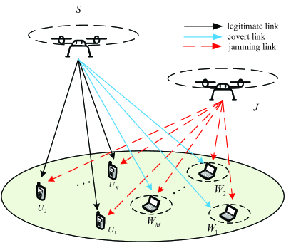
Figure 1: Dual-UAVs enabled covert communication system.

II-A System Model

As shown in Fig. 1, a flying UAV that works as a base station (${S}$) is transmitting confidential data to ${N_{U}}$ ground users ($U_{k},k=1,\cdots,N_{U}$). At the same time, $N_{W}$ terrestrial wardens ($W_{m},m=1,\cdots,N_{W}$) monitor the transmission of ${S}$ and ${S}$ tries to hide its transmission from all the wardens. A friendly jammer UAV (${J}$) sends jamming signals with the fixed power $P_{J}$ to fight with the wardens. All the wardens are assumed to be equipped with $K$ antennas and the other devices are equipped with a single antenna.

The flight period $T_{0}$ is equally divided into $N_{t}$ time slot as ${\delta_{t}}=\frac{T_{0}}{N_{t}}$, where $N_{t}$ is large enough to guarantee that the position of $S$ and $J$ can be seen as approximately fixed during each time slot [4]. The locations of all nodes in the system model are described using Cartesian coordinate system. It is assumed that ${S}$ and ${J}$ fly at a fixed altitude ${H_{S}}$ and ${H_{J}}$, respectively. The horizontal coordinate of $U_{k}$ and $W_{m}$ are expressed as ${{\bf{q}}_{{U_{k}}}}={\left[{{x_{{U_{k}}}},{y_{{U_{k}}}}}\right]^{T}}$ and ${{\bf{q}}_{{W_{m}}}}={\left[{{x_{{W_{m}}}},{y_{{W_{m}}}}}\right]^{T}}$, respectively. The horizontal locations of $S$ and $J$ are denoted as ${{\mathbf{q}}_{S}}{\left(n\right)}={\left[{{x_{S}}{\left(n\right)},{y_{S}}{\left(n\right)}}\right]^{T}}$ and ${{\mathbf{q}}_{J}}{\left(n\right)}={\left[{{x_{J}}{\left(n\right)},{y_{J}}{\left(n\right)}}\right]^{T}}$.

It assumed that the A2G links are LoS [33] and [34]. When $W_{m}$ is equipped with a single antenna $\left({K=1}\right)$, the channel coefficients from $S$ to the receivers are expressed as

$${h_{S{U_{k}}}}{\left(n\right)}=\sqrt{\frac{{{\rho_{0}}}}{{{{\left\|{{{\bf{q}}_{S}}\left(n\right)-{{\bf{q}}_{{U_{k}}}}}\right\|}^{2}}+H_{S}^{2}}}},$$ (1)

and

$${h_{S{W_{m}}}}{\left(n\right)}=\sqrt{\frac{{{\rho_{0}}}}{{{{\left\|{{{\bf{q}}_{S}}\left(n\right)-{{\bf{q}}_{{W_{m}}}}}\right\|}^{2}}+H_{S}^{2}}}},$$ (2)

respectively, where ${{\rho_{0}}}$ denotes the channel power gain at the reference distance. Similarly, the channel coefficients between $J$ and all the receivers at the $n$th slot are expressed as

$${h_{J{U_{k}}}}{\left(n\right)}=\sqrt{\frac{{{\rho_{0}}}}{{{{\left\|{{{\mathbf{q}}_{J}}{\left(n\right)}-{{\bf{q}}_{{U_{k}}}}}\right\|}^{2}}+H_{J}^{2}}}},$$ (3)

and

$${h_{J{W_{m}}}}{\left(n\right)}=\sqrt{\frac{{{\rho_{0}}}}{{{{\left\|{{{\mathbf{q}}_{J}}{\left(n\right)}-{{\bf{q}}_{{W_{m}}}}}\right\|}^{2}}+H_{J}^{2}}}},$$ (4)

respectively.

To take into account the uncertainty of wardens’ position in practical situations, the position of $W_{m}$ at $S$’s point of view is denoted as [30], [31]

$${{\bf{q}}_{{W_{m}}}}={{\bf{\hat{q}}}_{{W_{m}}}}+\Delta{{\bf{q}}_{{W_{m}}}},$$ (5)

where ${{\bf{\hat{q}}}_{{W_{m}}}}$ is the estimated position of $W_{m}$ and $\Delta{{\bf{q}}_{{W_{m}}}}$ denotes the estimation error follows

$${\left\|{\Delta{{\bf{q}}_{{W_{m}}}}}\right\|^{2}}\leq r_{m}^{2},$$ (6)

where ${r_{m}}$ is the estimation error radius for $W_{m}$.

II-B Detection Performance

The DEP is given as ${\xi_{m}}\left(n\right)={P_{{\rm{FA}}_{m}}}{\left(n\right)}+{P_{{\rm{MD}}_{m}}}{\left(n\right)}$, where ${P_{{\rm{FA}}_{m}}}{\left(n\right)}$ and ${P_{{\rm{MD}}_{m}}}{\left(n\right)}$ as $W_{m}$ denote the false alarm probability (FAP) and miss detection probability (MDP) respectively. To maximize the covert performance of the UAV system, the DEP of all the wardens should satisfy

$${\xi_{m}}\left(n\right)\geq 1-\varepsilon,\forall n,\forall m,$$ (7)

where $0\leq\varepsilon\leq 1$ is an sufficiently small positive value to reflect the requirement for covertness in the communication system.

Similar to [30], assuming that all wardens can only have a finite number of observations, they depend on $I$ times sensing of the received signal to determine whether $S$ is transmitting or not. The $i$th $\left({i=1,\cdots,I}\right)$ received signal on $W_{m}$ is denoted as

$$y_{{W_{m}}}^{i}\left(n\right)=\left\{{\begin{array}[]{*{20}{c}}{\sqrt{{P_{J}}}{h_{J{W_{m}}}}\left(n\right)x_{J}^{i}\left(n\right)+n_{{W_{m}}}^{i}\left(n\right)}&{{{\cal H}_{0}},}\\ {\sqrt{{P_{S}}\left(n\right)}{h_{S{W_{m}}}}\left(n\right)x_{S}^{i}\left(n\right)+\sqrt{{P_{J}}}{h_{J{W_{m}}}}\left(n\right)x_{J}^{i}\left(n\right)+n_{{W_{m}}}^{i}\left(n\right)}&{{{\cal H}_{1}},}\end{array}}\right.$$ (8)

where ${{\mathcal{H}_{0}}}$ and ${{\mathcal{H}_{1}}}$ represent the hypothesis that $S$ is not transmitting and transmitting, respectively, ${{P_{S}}{\left(n\right)}}$ represents $S$ transmit power, $x_{S}^{i}{\left(n\right)}$ and $x_{J}^{i}{\left(n\right)}$ are the $i$th transmitted signal following complex Gaussian distribution with zero and unit variance, and $n_{{W_{m}}}^{i}{\left(n\right)}$ is the complex additive Gaussian noise at $W_{m}$. The $i$th received signal at the $m$th warden follows [32]

$$y_{{W_{m}}}^{i}{\left(n\right)}\sim\left\{{\begin{array}[]{*{20}{l}}{CN\left({0,\sigma_{0}^{2}}\right),}&{{\mathcal{H}_{0}},}\\ {CN\left({0,\sigma_{1}^{2}}\right),}&{{\mathcal{H}_{1}},}\end{array}}\right.$$ (9)

where $\sigma_{0}^{2}={P_{J}}{\left|{{h_{J{W_{m}}}}{\left(n\right)}}\right|^{2}}+{\sigma^{2}}$, $\sigma_{1}^{2}={P_{S}}{\left(n\right)}{\left|{{h_{S{W_{m}}}}{\left(n\right)}}\right|^{2}}+{P_{J}}{\left|{{h_{J{W_{m}}}}{\left(n\right)}}\right|^{2}}+{\sigma^{2}}$, and ${\sigma^{2}}$ is the noise power. Then the observed matrix at $W_{m}$ is expressed as

$${{\mathbf{y}}_{{W_{m}}}}{\left(n\right)}={\left[{y_{{W_{m}}}^{1}{\left(n\right)},\cdots,y_{{W_{m}}}^{I}{\left(n\right)}}\right]^{T}}\in{\mathbb{C}^{I}}.$$ (10)

The worst-scenario is considered where $W_{m}$ adopts the likelihood ratio test for minimizing its DEP, which is expressed as [35],

$$\frac{{f\left({{{\mathbf{y}}_{{W_{m}}}}{\left(n\right)}|{\mathcal{H}_{1}}}\right)}}{{f\left({{{\mathbf{y}}_{{W_{m}}}}{\left(n\right)}|{\mathcal{H}_{0}}}\right)}}\mathop{\mathop{\gtrless}\limits_{{\mathcal{D}_{0}}}}\limits^{{\mathcal{D}_{1}}}1,$$ (11)

where ${\mathcal{D}_{0}}$ and ${\mathcal{D}_{1}}$ represent the $W_{m}$’s decision, $f\left({{{\mathbf{y}}_{{W_{m}}}}{\left(n\right)}|{\mathcal{H}_{0}}}\right)$ and $f\left({{{\mathbf{y}}_{{W_{m}}}}{\left(n\right)}|{{\mathcal{H}_{1}}}}\right)$ are the likelihood function under ${\mathcal{H}_{0}}$ and ${\mathcal{H}_{1}}$, respectively, which are expressed as

$$f\left({{{\mathbf{y}}_{{W_{m}}}}{\left(n\right)}|{{\mathcal{H}_{j}}}}\right)=\frac{1}{{{{\left({\pi\sigma_{j}^{2}}\right)}^{I}}}}\prod\limits_{i=1}^{I}{\exp\left({-\frac{{{{\left|{y_{{W_{m}}}^{i}{\left(n\right)}}\right|}^{2}}}}{{\sigma_{j}^{2}}}}\right)},$$ (12)

where $j\in\left\{{0,1}\right\}$. Following (11) and (12), the log-likelihood ratio is obtained as

$${\ell_{m}}{\left(n\right)} =\ln\left({\frac{{f\left({{{\mathbf{y}}_{{W_{m}}}}{\left(n\right)}|{{\mathcal{H}_{1}}}}\right)}}{{f\left({{{\mathbf{y}}_{{W_{m}}}}{\left(n\right)}|{{\mathcal{H}_{0}}}}\right)}}}\right)$$ (13)

$$=I\ln\left({\frac{{\sigma_{0}^{2}}}{{\sigma_{1}^{2}}}}\right)+\left({\frac{1}{{\sigma_{0}^{2}}}-\frac{1}{{\sigma_{1}^{2}}}}\right)\sum\limits_{i=1}^{I}{{{\left|{y_{{W_{m}}}^{i}{\left(n\right)}}\right|}^{2}}},$$

and the optimal decision rule at $W_{m}$ is given by

$${\ell_{m}}{\left(n\right)}\mathop{\mathop{\gtrless}\limits_{{\mathcal{D}_{0}}}}\limits^{{\mathcal{D}_{1}}}0\Leftrightarrow{E_{m}}\left(n\right)\mathop{\mathop{\gtrless}\limits_{{\mathcal{D}_{0}}}}\limits^{{\mathcal{D}_{1}}}\zeta,$$ (14)

respectively, where ${E_{m}}\left(n\right)=\sum\limits_{i=1}^{I}{{{\left|{y_{{W_{m}}}^{i}\left(n\right)}\right|}^{2}}}$ signify the sum power of each received symbol at $W_{m}$ and $\zeta=I\ln\left({\frac{{\sigma_{1}^{2}}}{{\sigma_{0}^{2}}}}\right){\left({\frac{1}{{\sigma_{0}^{2}}}-\frac{1}{{\sigma_{1}^{2}}}}\right)^{-1}}$ denotes the dection threshold for ${E_{m}}\left(n\right)$. Based on [21], ${E_{m}}\left(n\right)\sim\frac{{\sigma_{j}^{2}}}{2}\chi$, where $\chi$ represents denotes a chi-squared random variable (RV) with $2I$. Then, following (14), ${P_{{\rm{FA}}_{m}}}{\left(n\right)}$ is obtained as

$${P_{{\rm{FA}}_{m}}}{\left(n\right)} =\Pr\left\{{{E_{m}}\left(n\right)\geq\zeta|{{\cal H}_{0}}}\right\}$$ (15)

$$=\Pr\left\{{\chi\geq\frac{{2\zeta}}{{\sigma_{0}^{2}}}}\right\}$$

$$=1-\frac{1}{{\Gamma\left(I\right)}}\Upsilon\left({I,\frac{\zeta}{{\sigma_{0}^{2}}}}\right),$$

where $\Upsilon\left({z,x}\right)=\int_{0}^{x}{{t^{z-1}}{e^{-t}}dt}$ is the lower incomplete Gamma function, as defined by [36, (8.350.1)]. With the same method, we have

$${P_{{\rm{MD}}_{m}}}{\left(n\right)}=\frac{1}{{\Gamma\left(I\right)}}\Upsilon\left({I,\frac{\zeta}{{\sigma_{1}^{2}}}}\right).$$ (16)

Thus, the DEP of $W_{m}$ is obtained as

$${\xi_{m}}\left(n\right)=1+\frac{1}{{\Gamma\left(I\right)}}\left({\Upsilon\left({I,\frac{\zeta}{{\sigma_{1}^{2}}}}\right)-\Upsilon\left({I,\frac{\zeta}{{\sigma_{0}^{2}}}}\right)}\right).$$ (17)

II-C Problem Formulation

Assume that the interference signals emitted by $J$ is a Gaussian pseudo-random sequence and can be perfect deleted from the received signals at all the ground user, like [37], [38, 39]. Then the achievable rate of $U_{k}$ is expressed as

$${R_{k}}{\left(n\right)}={\log_{2}}\left({1+{\gamma_{k}}\left(n\right)}\right),$$ (18)

where ${\gamma_{k}}\left(n\right)={\rho_{S}}\left(n\right){\left|{{h_{S{U_{k}}}}\left(n\right)}\right|^{2}}$ and ${\rho_{S}}\left(n\right)=\frac{{{P_{S}}\left(n\right)}}{{{\sigma^{2}}}}$. Then the average achievable covert rate of $U_{k}$ is expressed as

$${\bar{R}_{k}}=\frac{1}{N}\sum\limits_{n=1}^{N}{{R_{k}}\left(n\right)}.$$ (19)

In this work, the minimum average covert rate is maximized with respect to the trajectory and transmit power of $S$ and the trajectory of $J$. Let ${{\mathbf{P}}_{S}}=\left\{{{P_{S}}{\left(n\right)},\forall n}\right\}$, ${{\mathbf{Q}}_{S}}=\left\{{{{\mathbf{q}}_{S}}{\left(n\right)},\forall n}\right\}$, ${{\mathbf{Q}}_{J}}=\left\{{{{\mathbf{q}}_{J}}{\left(n\right)},\forall n}\right\}$, we have the following optimaiztion problem

$$\mathcal{P}_{1}: \mathop{\max}\limits_{{{\mathbf{P}}_{S}},{{\mathbf{Q}}_{S}},{{\mathbf{Q}}_{J}}}\;\mathop{\min}\limits_{1\leq k\leq K}{{\bar{R}}_{k}}$$ (20a)

$${\mathrm{s.t.}}\; {\xi_{m}}\left(n\right)\geq 1-\varepsilon,\forall n,\forall m,$$ (20b)

$${P_{S}}\left(n\right)\leq{P_{\max}},\forall n,$$ (20c)

$${{\bf{q}}_{S}}\left(1\right)={{\bf{q}}_{S}^{\rm{I}}},{{\bf{q}}_{S}}\left(N\right)={{\bf{q}}_{S}^{\rm{F}}},$$ (20d)

$${{\bf{q}}_{J}}\left(1\right)={{\bf{q}}_{J}^{\rm{I}}},{{\bf{q}}_{J}}\left(N\right)={{\bf{q}}_{J}^{\rm{F}}},$$ (20e)

$$\left\|{{{\bf{q}}_{S}}\left({n+1}\right)-{{\bf{q}}_{S}}\left(n\right)}\right\|\leq{V_{S,\max}}{\delta_{t}},n=1,\cdots,{N_{t}}-1,$$ (20f)

$$\left\|{{{\bf{q}}_{J}}\left({n+1}\right)-{{\bf{q}}_{J}}\left(n\right)}\right\|\leq{V_{J,\max}}{\delta_{t}},n=1,\cdots,{N_{t}}-1,$$ (20g)

where (20b) is the covert constraint, (20c) is the peak power constraint of S where $P_{max}$ signifies maximum transmit power of $S$, (20d) and (20e) denote the constraints on the take-off and landing positions of $S$ and $J$, respectively, where ${{\bf{q}}_{S}^{\rm{I}}}$ and ${{\bf{q}}_{S}^{\rm{F}}}$ are the take-off and landing positions of $S$, respectively, and ${{\bf{q}}_{J}^{\rm{I}}}$ and ${{\bf{q}}_{J}^{\rm{F}}}$ are the take-off and landing positions of $J$, respectively, (20f) and (20g) depicts the maximum flight distance between adjacent time slots of both UAVs where ${V_{S,\max}}$ and ${V_{J,\max}}$ denote the maximum velocity of $S$ and $J$, respectively.

Problem $\mathcal{P}_{1}$ is a multivariate coupled non-convex problem. Several factors make $\mathcal{P}_{1}$ challenging to solve. First, the objective function ${\bar{R}_{k}}$ in (20a) is a non-convex with respect to variable ${{\mathbf{P}}_{S}}$, ${{\mathbf{Q}}_{S}}$ and ${{\mathbf{Q}}_{J}}$. Second, the covert constraint (20b) is a non-convex constraint and it has highly complicated with respect to all the optimization variables. Moreover, (20b) contains location estimate for all the wardens, which will change the number of constraints from finite to infinite.

In the following section, a SCA-based algorithm is proposed for handling the non-convexity of problem $\mathcal{P}_{1}$.

III Covert Rate Maximization

III-A Tractable Covertness Constraint

Due to the complexity of constraint (20b) and the coupled variables, it is impossible to perform a direct convexity operation on $\mathcal{P}_{1}$. The following Lemma provides an alternative to obtain a simpler equivalent form.

Lemma 1.

The DEP of $W_{m}$ is obtained as monotonically decreasing respect to ${{\gamma_{m,1}}\left(n\right)}=\frac{{{P_{S}}\left(n\right){{\left|{{h_{S{W_{m}}}}\left(n\right)}\right|}^{2}}}}{{{P_{J}}{{\left|{{h_{J{W_{m}}}}\left(n\right)}\right|}^{2}}+{\sigma^{2}}}}$.

Proof.

Based on the definition of $\zeta$ and ${\sigma_{j}^{2}}$, we obtain

$$\frac{\zeta}{{\sigma_{0}^{2}}}=\frac{{I\left({1+{\gamma_{m,1}}\left(n\right)}\right)\ln\left({1+{\gamma_{m,1}}\left(n\right)}\right)}}{{{\gamma_{m,1}}\left(n\right)}}$$ (21)

and

$$\frac{\zeta}{{\sigma_{1}^{2}}}=\frac{{I\ln\left({1+{\gamma_{m,1}}\left(n\right)}\right)}}{{{\gamma_{m,1}}\left(n\right)}},$$ (22)

where ${{\gamma_{m,1}}\left(n\right)}=\frac{{{P_{S}}\left(n\right){{\left|{{h_{S{W_{m}}}}\left(n\right)}\right|}^{2}}}}{{{P_{J}}{{\left|{{h_{J{W_{m}}}}\left(n\right)}\right|}^{2}}+{\sigma^{2}}}}$ denotes the SINR of $W_{m}$. Then based on $\Upsilon\left({z,x}\right)=\int_{0}^{x}{{t^{z-1}}{e^{-t}}dt}$, the DEP is rewritten as

$${\xi_{m}}\left(n\right)=1-\frac{1}{{\Gamma\left(I\right)}}\int_{\frac{{I\ln\left({1+{\gamma_{m,1}}\left(n\right)}\right)}}{{{\gamma_{m,1}}\left(n\right)}}}^{\frac{{I\left({1+{\gamma_{m,1}}\left(n\right)}\right)\ln\left({1+{\gamma_{m,1}}\left(n\right)}\right)}}{{{\gamma_{m,1}}\left(n\right)}}}{{t^{I-1}}{e^{-t}}dt}.$$ (23)

One can observe that the ${\frac{{I\ln\left(1+{{{\gamma_{m,1}}\left(n\right)}}\right)}}{{{{\gamma_{m,1}}\left(n\right)}}}}\leq 0$ and ${\frac{{I\left({1+{{\gamma_{m,1}}\left(n\right)}}\right)\ln\left({1+{{\gamma_{m,1}}\left(n\right)}}\right)}}{{{{\gamma_{m,1}}\left(n\right)}}}}\geq 0$, which signifies are monotonically decreasing or increasing respect to ${{{\gamma_{m,1}}\left(n\right)}>0}$. Thus, ${\xi_{m}}\left(n\right)$ is monotonically decreasing respect to ${{{\gamma_{m,1}}\left(n\right)}}$. ∎

Since a given covertness requirement must to be satisfied, given in (7), then we have

$${{\gamma_{m,1}}\left(n\right)}\leq{\gamma_{\max,1}},$$ (24)

where ${\gamma_{\max,1}}$ is maximum value of ${{\gamma_{m,1}}\left(n\right)}$, which can be obtained by utilizing bisection search method.

III-B SCA-Based Joint Optimization Algorithm

By replace (20b) for (24) and introduce a slack variable $\eta$, the problem $\mathcal{P}_{1}$ can be equivalently transformed into a more tractable formulation, namely,

$$\mathcal{P}_{1.1}: \mathop{\max}\limits_{{{\mathbf{P}}_{S}},{{\mathbf{Q}}_{S}},{{\mathbf{Q}}_{J}},\eta}\;\eta$$ (25a)

$${\mathrm{s.t.}}\; \eta\leq\frac{1}{N}\sum\limits_{n=1}^{N}{{R_{k}}{\left(n\right)}},\forall k,$$ (25b)

$${{\gamma_{m,1}}\left(n\right)}\leq{\gamma_{\max,1}},\forall n,\forall m,$$ (25c)

$$(\textrm{\ref{P1c}})-(\textrm{\ref{P1g}}).$$ (25d)

It should be noted that (25b) and (25c) are non-convex.

To cope with the non-convexity of (25b), the lower bound of ${R_{k}}\left(n\right)$ is obtained as

$${R_{k}}\left(n\right) \geq{\log_{2}}\left({1+\frac{{{\gamma_{0}}{P_{S}}\left(n\right)}}{{{d_{k}}\left(n\right)}}}\right)$$ (26)

$$={\log_{2}}\left({{\gamma_{0}}{P_{S}}\left(n\right)+{d_{k}}\left(n\right)}\right)-{\log_{2}}\left({{d_{k}}\left(n\right)}\right)$$

$$\mathop{\geq}\limits^{\left(a\right)}{\log_{2}}\left({{\gamma_{0}}{P_{S}}\left(n\right)+{d_{k}}\left(n\right)}\right)-{\log_{2}}\left({d_{k}^{l}\left(n\right)}\right)$$

$$-\frac{{{d_{k}}\left(n\right)-d_{k}^{l}\left(n\right)}}{{d_{k}^{l}\left(n\right)\ln\left(2\right)}}$$

$$\buildrel\Delta\over{=}R_{k}^{\rm{L},1}\left(n\right),$$

where ${d_{k}}\left(n\right)$ is a new slack variable, which must satisfy

$${d_{k}}\left(n\right)\geq{\left\|{{{\bf{q}}_{S}}\left(n\right)-{{\bf{u}}_{k}}}\right\|^{2}}+H_{S}^{2},\forall n,\forall k,$$ (27)

step $\left(a\right)$ is obtained by SCA, $d_{k}^{l}\left(n\right)$ is a feasible point derived from the $l$th iteration. Then, (25b) is approximately transformed into

$$\eta\leq\frac{1}{N}\sum\limits_{n=1}^{N}{R_{k}^{\rm{L},1}\left(n\right)},\forall k,$$ (28)

Similarly, a slack variable ${b_{m}}\left(n\right)$ is introduced for handling the non-convexity of (25c), which is reformulated as

$$\frac{{{P_{S}}\left(n\right){\rho_{0}}}}{{{{\left\|{{{\bf{q}}_{S}}\left(n\right)-{{\bf{q}}_{{W_{m}}}}}\right\|}^{2}}+H_{S}^{2}}}\leq{\gamma_{\max,1}}{b_{m}}\left(n\right),\forall n,\forall m,$$ (29)

where ${b_{m}}\left(n\right)$ satisfy

$${b_{m}}\left(n\right)\leq\frac{{{P_{J}}{\rho_{0}}}}{{{{\left\|{{{\bf{q}}_{J}}\left(n\right)-{{\bf{q}}_{{W_{m}}}}}\right\|}^{2}}+H_{J}^{2}}}+{\sigma^{2}},\forall n,\forall m.$$ (30)

By introducing slack variables ${c_{m}}\left(n\right)$ and ${v_{m}}\left(n\right)$ the constraint is further reformulated as

$$\frac{{{\rho_{0}}{P_{S}}\left(n\right)}}{{{v_{m}}\left(n\right)}} \leq{\gamma_{\max,1}}{b_{m}}\left(n\right),\forall n,\forall m,$$ (31a)

$${b_{m}}\left(n\right) \leq\frac{{{\rho_{0}}{P_{J}}}}{{{c_{m}}\left(n\right)}}+{\sigma^{2}},\forall n,\forall m,$$ (31b)

$${c_{m}}\left(n\right) \geq{\left\|{{{\bf{q}}_{J}}\left(n\right)-{{\bf{q}}_{{W_{m}}}}}\right\|^{2}}+H_{J}^{2},\forall n,\forall m,$$ (31c)

$${v_{m}}\left(n\right) \leq{\left\|{{{\bf{q}}_{S}}\left(n\right)-{{\bf{q}}_{{W_{m}}}}}\right\|^{2}}+H_{S}^{2},\forall n,\forall m,$$ (31d)

To handle the mutually coupled variables, (31a) is written as

$$\ln\left({{\rho_{0}}{P_{S}}\left(n\right)}\right)\leq\ln\left({{\gamma_{\max,1}}{b_{m}}\left(n\right)}\right)+\ln\left({{v_{m}}\left(n\right)}\right),\forall n,\forall m.$$ (32)

By utilizing SCA, we obtain

$$\ln\left({{\rho_{0}}{P_{S}}\left(n\right)}\right) \leq\ln\left({{\rho_{0}}P_{S}^{l}\left(n\right)}\right)+\frac{{{P_{S}}\left(n\right)-P_{S}^{l}\left(n\right)}}{{P_{S}^{l}\left(n\right)}}\buildrel\Delta\over{=}A\left(n\right),$$ (33)

$$\frac{1}{{{c_{m}}\left(n\right)}} \geq\frac{1}{{c_{m}^{l}\left(n\right)}}-\frac{1}{{{{\left({c_{m}^{l}\left(n\right)}\right)}^{2}}}}\left({{c_{m}}\left(n\right)-c_{m}^{l}\left(n\right)}\right)\buildrel\Delta\over{=}B\left(n\right),$$ (34)

respectively, where $P_{S}^{l}\left(n\right)$ and $c_{m}^{l}\left(n\right)$ are feasible point obtained by the $l$th iteration, respectively, Then (31a) and (31b) are approximately transformed into

$$A\left(n\right)\leq\ln\left({{\gamma_{\max,1}}{b_{m}}\left(n\right)}\right)+\ln\left({{v_{m}}\left(n\right)}\right),\forall n,\forall m,$$ (35)

and

$${b_{m}}\left(n\right)\leq{\rho_{0}}{P_{J}}{B_{m}}\left(n\right)+{\sigma^{2}},\forall n,\forall m,$$ (36)

respectively.

It must be noted that constraints (31c) and (31d) still intractable due to $\Delta{{\bf{q}}_{{W_{m}}}}$.The triangle inequality is utilized to obtain the upper bound, which is expressed as [43]

$$\left\|{{{\bf{q}}_{J}}\left(n\right)-{{\bf{q}}_{{W_{m}}}}}\right\| =\left\|{{{\bf{q}}_{J}}\left(n\right)-{{{\bf{\hat{q}}}}_{{W_{m}}}}-\Delta{{\bf{q}}_{{W_{m}}}}}\right\|$$ (37)

$$\leq\left\|{{{\bf{q}}_{J}}\left(n\right)-{{{\bf{\hat{q}}}}_{{W_{m}}}}}\right\|+\left\|{\Delta{{\bf{q}}_{{W_{m}}}}}\right\|$$

$$\leq\left\|{{{\bf{q}}_{J}}\left(n\right)-{{{\bf{\hat{q}}}}_{{W_{m}}}}}\right\|+{r_{m}}.$$

Then the constraint (31c) is approximated by

$${c_{m}}{\left(n\right)}\geq{\left({\left\|{{{\mathbf{q}}_{J}}{\left(n\right)}-{{{\bf{\hat{q}}}}_{{W_{m}}}}}\right\|+{r_{m}}}\right)^{2}}+H_{J}^{2},\forall n,\forall m,$$ (38)

By introducing slack variables ${{\theta_{m}}\left(n\right)}$ and applying the S-procedure technique, constraint (31d) is equivalently transformed into

$$\left({\begin{array}[]{*{20}{c}}{\left({1+{\theta_{m}}{\left(n\right)}}\right){\mathbf{I}}}&{-\left({{{\mathbf{q}}_{S}}{\left(n\right)}-{{{\bf{\hat{q}}}}_{{W_{m}}}}}\right)}\\ {-{{\left({{{\mathbf{q}}_{S}}{\left(n\right)}-{{{\bf{\hat{q}}}}_{{W_{m}}}}}\right)}^{T}}}&{{{\left\|{{{\mathbf{q}}_{S}}{\left(n\right)}-{{{\bf{\hat{q}}}}_{{W_{m}}}}}\right\|}^{2}}+{\iota_{m}}{\left(n\right)}}\end{array}}\right)\succcurlyeq 0,\forall n,\forall m,$$ (39c)

$${\theta_{m}}\left(n\right)\geq 0,\forall n,\forall m,$$ (39d)

where ${\mathbf{I}}$ denotes the $2\times 2$ identity matrix, ${\iota_{m}}{\left(n\right)}\triangleq H_{S}^{2}-{v_{m}}{\left(n\right)}-{\theta_{m}}{\left(n\right)}r_{m}^{2}$. By utilizing SCA, we obtain

$${\left\|{{{\bf{q}}_{S}}\left(n\right)-{{{\bf{\hat{q}}}}_{{W_{m}}}}}\right\|^{2}} \geq{\left\|{{\bf{q}}_{S}^{l}\left(n\right)-{{{\bf{\hat{q}}}}_{{W_{m}}}}}\right\|^{2}}$$ (40)

$$+2{\left({{\bf{q}}_{S}^{l}\left(n\right)-{{{\bf{\hat{q}}}}_{{W_{m}}}}}\right)^{T}}\left({{{\bf{q}}_{S}}\left(n\right)-{\bf{q}}_{S}^{l}\left(n\right)}\right)$$

$$\buildrel\Delta\over{=}{C_{m}}\left(n\right),$$

where ${\bf{q}}_{S}^{l}\left(n\right)$ is a feasible point derived from the $l$th iteration. Then (39c) is approximated by

$$\left({\begin{array}[]{*{20}{c}}{\left({1+{\theta_{m}}\left(n\right)}\right){\mathbf{I}}}&{-\left({{{\mathbf{q}}_{S}}\left(n\right)-{{{\mathbf{\hat{q}}}}_{{W_{m}}}}}\right)}\\ {-{{\left({{{\mathbf{q}}_{S}}\left(n\right)-{{{\mathbf{\hat{q}}}}_{{W_{m}}}}}\right)}^{T}}}&{{C_{m}}\left(n\right)+{\iota_{m}}\left(n\right)}\end{array}}\right)\succcurlyeq 0,\forall n,\forall m.$$ (41)

Let ${\mathbf{b}}=\left\{{{b_{m}}\left(n\right),\forall n,\forall m}\right\}$, ${\mathbf{c}}=\left\{{{c_{m}}{\left(n\right)},\forall n,\forall m}\right\}$, ${\mathbf{d}}=\left\{{{d_{k}}{\left(n\right)},\forall n,\forall k}\right\}$, ${\mathbf{v}}=\left\{{{v_{m}}{\left(n\right)},\forall n,\forall m}\right\}$, and ${\mathbf{\Theta}}=\left\{{{\theta_{m}}{\left(n\right)},\forall n,\forall m}\right\}$, problem $\mathcal{P}_{1.1}$ is rewritten as

$$\mathcal{P}_{1.2}: \mathop{\max}\limits_{{{\mathbf{P}}_{S}},{{\mathbf{Q}}_{S}},{{\mathbf{Q}}_{J}},{\mathbf{b}},{\mathbf{c}},{\mathbf{v}},{\mathbf{d}},{\mathbf{\Theta}},\eta}\;\eta$$ (42a)

$${\mathrm{s.t.}}\; (\textrm{\ref{P1.1d}}),(\textrm{\ref{P1.1b3}}),(\textrm{\ref{P1.1b4}}),(\textrm{\ref{eq:1c3a4}}),(\textrm{\ref{eq:1c3b3}}),(\textrm{\ref{eq:1c3c2}}),(\textrm{\ref{eq:1c3d2}}),(\textrm{\ref{eq:eq:1c3d4}}).$$ (42b)

Now $\mathcal{P}_{1.2}$ is a convex problem, and it can be efficiently solved by CVX toolbox [40].

Input: Initialization of feasible points.

while $R\left({{\mathbf{Q}}_{S}^{l},{\mathbf{Q}}_{J}^{l},{\mathbf{P}}_{S}^{l}}\right)-R\left({{\mathbf{Q}}_{S}^{l-1},{\mathbf{Q}}_{J}^{l-1},{\mathbf{P}}_{S}^{l-1}}\right)\leq{\hat{\xi}}$ do

       1. Solve $\mathcal{P}_{1.2}$;

       2. $l=l+1$;

       3. Calculate the objective value $R\left({{\mathbf{Q}}_{S}^{l},{\mathbf{Q}}_{J}^{l},{\mathbf{P}}_{S}^{l}}\right)$.

end while

Output: $R\left({{\mathbf{Q}}_{S}^{l},{\mathbf{Q}}_{J}^{l},{\mathbf{P}}_{S}^{l}}\right)$ with ${\mathbf{Q}}_{S}^{*}={\mathbf{Q}}_{S}^{l},\;{\mathbf{Q}}_{J}^{*}={\mathbf{Q}}_{J}^{l},\;{\mathbf{P}}_{S}^{*}={\mathbf{P}}_{S}^{l}$.

Algorithm 1 Proposed Algorithm for Non-Convex Problem $\mathcal{P}_{1}$

To solve $\mathcal{P}_{1}$, we propose an iterative algorithm whose details of the entire iteration are summarized in Algorithm 1, where the tolerance of the convergence of the algorithm is denoted as $\hat{\xi}$.

III-C Convergence and Complexity Analysis

By following the proof of [44], it is straightforward to show that the solution generated by Algorithm 1 converges to a KKT solution of problem $\mathcal{P}_{1}$.

The computational complexity of our proposed Algorithm 1 lies in solving SDP $\mathcal{P}_{1.2}$. Based on [45, Theorem 1], the computational complexity for finding an ${\hat{\varepsilon}}$-optimal solution of problem $\mathcal{P}_{1.2}$ is $\mathcal{O}\left({\sqrt{3{N_{t}}{N_{W}}+{A_{t}}}\left({{3^{3}}{N_{t}}{N_{W}}+9{A_{t}}{N_{t}}{N_{W}}+A_{t}^{2}}\right)\ln\frac{1}{{\hat{\varepsilon}}}}\right)$, where ${A_{t}}={N_{U}}+4{N_{t}}{N_{W}}+{N_{t}}{N_{U}}+3{N_{t}}+6$ is the number of constraints that is not a SDP cone. Then, the computational complexity of Algorithm 1 is ${N_{num}}\mathcal{O}\left({\sqrt{3{N_{t}}{N_{W}}+{A_{t}}}\left({{3^{3}}{N_{t}}{N_{W}}+9{A_{t}}{N_{t}}{N_{W}}+A_{t}^{2}}\right)\ln\frac{1}{{\hat{\varepsilon}}}}\right)$, where ${N_{num}}$ is the maximal iteration number of Algorithm 1.

IV All The Wardens Equipped with Multiple Antennas

When all the wardens equipped with multiple antennas $\left({K>1}\right)$, the channel coefficients between the transmitters and $W_{m}$ at the $n$th slot are expressed as

$${{\mathbf{h}}_{S{W_{m}}}}{\left(n\right)}={\left[{{h_{S{W_{m}}}}{\left(n\right)},\cdots,{h_{S{W_{m}}}}{\left(n\right)}}\right]^{T}}\in{\mathbb{R}^{K}},$$ (43)

and

$${{\mathbf{h}}_{J{W_{m}}}}{\left(n\right)}={\left[{{h_{J{W_{m}}}}{\left(n\right)},\cdots,{h_{J{W_{m}}}}{\left(n\right)}}\right]^{T}}\in{\mathbb{R}^{K}},$$ (44)

respectively.

The received signal at $W_{m}$ as [21]

$${{\mathbf{Y}}_{{W_{m}}}}{\left(n\right)}=\left[{{\mathbf{y}}_{{W_{m}}}^{1}{\left(n\right)},\cdots,{\mathbf{y}}_{{W_{m}}}^{I}{\left(n\right)}}\right]\in{\mathbb{C}^{K\times I}},$$ (45)

where ${\bf{y}}_{{W_{m}}}^{i}\left(n\right)$ is given in

$${\bf{y}}_{{W_{m}}}^{i}\left(n\right)=\left\{{\begin{array}[]{*{20}{c}}{\sqrt{{P_{J}}}{{\bf{h}}_{J{W_{m}}}}\left(n\right)x_{J}^{i}\left(n\right)+{\bf{n}}_{{W_{m}}}^{i}\left(n\right),}&{{{\cal H}_{0}},}\\ {\sqrt{{P_{S}}\left(n\right)}{{\bf{h}}_{S{W_{m}}}}\left(n\right)x_{S}^{i}\left(n\right)+\sqrt{{P_{J}}}{{\bf{h}}_{J{W_{m}}}}\left(n\right)x_{J}^{i}\left(n\right)+{\bf{n}}_{{W_{m}}}^{i}\left(n\right),}&{{{\cal H}_{1}},}\end{array}}\right.$$ (46)

and ${\mathbf{n}}_{{W_{m}}}^{i}{\left(n\right)}={\left[{n_{{W_{m}}}^{i}{\left(n\right)},\cdots,n_{{W_{m}}}^{i}{\left(n\right)}}\right]^{T}}\in{\mathbb{C}^{K}}$. The $i$th received signal at $W_{m}$ follows the following distribution

$${\mathbf{y}}_{{W_{m}}}^{i}{\left(n\right)}\sim\left\{{\begin{array}[]{*{20}{l}}{CN\left({{\mathbf{0}},{{\mathbf{K}}_{0}}{\left(n\right)}}\right)}&{{\mathcal{H}_{0}},}\\ {CN\left({{\mathbf{0}},{{\mathbf{K}}_{1}}{\left(n\right)}}\right)}&{{\mathcal{H}_{1}},}\end{array}}\right.$$ (47)

where ${{\mathbf{K}}_{0}}{\left(n\right)}={\sigma^{2}}{\mathbf{I}}+{P_{J}}{{\mathbf{h}}_{J{W_{m}}}}{\left(n\right)}{\mathbf{h}}_{J{W_{m}}}^{H}{\left(n\right)}$ and ${{\mathbf{K}}_{1}}{\left(n\right)}={\sigma^{2}}{\mathbf{I}}+{P_{J}}{{\mathbf{h}}_{J{W_{m}}}}{\left(n\right)}{\mathbf{h}}_{J{W_{m}}}^{H}{\left(n\right)}$
$+{P_{S}}{\left(n\right)}{{\mathbf{h}}_{S{W_{m}}}}{\left(n\right)}{\mathbf{h}}_{S{W_{m}}}^{H}{\left(n\right)}$. Then the PDF of ${{\mathbf{Y}}_{{W_{m}}}}{\left(n\right)}$ is expressed as

$$f\left({{{\bf{Y}}_{{W_{m}}}}\left(n\right)|{{\cal H}_{j}}}\right) =\prod\limits_{i=1}^{I}{\frac{1}{{{\pi^{K}}\det\left({{{\bf{K}}_{j}}\left(n\right)}\right)}}\exp\left({-{\bf{y}}_{{W_{m}}}^{i}{{\left(n\right)}^{H}}{\bf{K}}_{j}^{-1}\left(n\right){\bf{y}}_{{W_{m}}}^{i}\left(n\right)}\right)}$$ (48)

$$={\left({\frac{1}{{{\pi^{K}}\det\left({{{\bf{K}}_{j}}\left(n\right)}\right)}}}\right)^{I}}\exp\left({-{\rm{Tr}}\left({{\bf{K}}_{j}^{-1}\left(n\right){{\bf{Y}}_{{W_{m}}}}\left(n\right){{\bf{Y}}_{{W_{m}}}}{{\left(n\right)}^{H}}}\right)}\right),$$

where $\det\left({{{\bf{K}}_{1}}\left(n\right)}\right)=\left({{\sigma^{2}}+{P_{J}}{{\left\|{{{\bf{h}}_{J{W_{m}}}}\left(n\right)}\right\|}^{2}}+{P_{S}}\left(n\right){{\left\|{{{\bf{h}}_{S{W_{m}}}}\left(n\right)}\right\|}^{2}}}\right){\sigma^{2\left({K-1}\right)}}$, $\det\left({{{\bf{K}}_{0}}\left(n\right)}\right)=\left({{\sigma^{2}}+{P_{J}}{{\left\|{{{\bf{h}}_{J{W_{m}}}}\left(n\right)}\right\|}^{2}}}\right){\sigma^{2\left({K-1}\right)}}$, ${{\bf{K}}_{1}}\left(n\right)={\sigma^{2}}{\bf{I}}+{{\bf{g}}_{m}}\left(n\right){\bf{g}}_{m}^{H}\left(n\right)$, ${\bf{K}}_{1}^{-1}\left(n\right)=\frac{1}{{{\sigma^{2}}}}\left({{\bf{I}}-\frac{{{{\bf{g}}_{m}}\left(n\right){\bf{g}}_{m}^{H}\left(n\right)}}{{{\sigma^{2}}+{{\left\|{{{\bf{g}}_{m}}\left(n\right)}\right\|}^{2}}}}}\right)$, where ${\mathbf{K}}_{0}^{-1}{\left(n\right)}$, ${\mathbf{K}}_{1}^{-1}{\left(n\right)}$ is obtained using Woodbury Matrix Identity for matrix inversion [41], ${{\mathbf{g}}_{m}}{\left(n\right)}={\left[{{G_{m}}{\left(n\right)},\cdots,{G_{m}}{\left(n\right)}}\right]^{T}}\in{\mathbb{R}^{K}}$, and ${G_{m}}{\left(n\right)}\triangleq\sqrt{{P_{J}}{{\left|{{h_{J{W_{m}}}}{\left(n\right)}}\right|}^{2}}+{P_{S}}{\left(n\right)}{{\left|{{h_{S{W_{m}}}}{\left(n\right)}}\right|}^{2}}}$.

Similarly, the log-likelihood ratio is denoted as

$${\ell_{m}}{\left(n\right)}= \ln\left({\frac{{f\left({{{\mathbf{Y}}_{{W_{m}}}}{\left(n\right)}|{\mathcal{H}_{1}}}\right)}}{{f\left({{{\mathbf{Y}}_{{W_{m}}}}{\left(n\right)}|{\mathcal{H}_{0}}}\right)}}}\right)$$ (49)

$$= I\ln\left({\frac{{\det\left({{{\mathbf{K}}_{0}}{\left(n\right)}}\right)}}{{\det\left({{{\mathbf{K}}_{1}}{\left(n\right)}}\right)}}}\right)+\frac{1}{{{\sigma^{2}}}}\frac{{{{\left\|{{\mathbf{g}}_{m}^{H}{\left(n\right)}{{\mathbf{Y}}_{{W_{m}}}}{\left(n\right)}}\right\|}^{2}}}}{{{\sigma^{2}}+{{\left\|{{{\mathbf{g}}_{m}}{\left(n\right)}}\right\|}^{2}}}}-\frac{1}{{{\sigma^{2}}}}\frac{{{{\left\|{{\mathbf{h}}_{J{W_{m}}}^{H}{\left(n\right)}{{\mathbf{Y}}_{{W_{m}}}}{\left(n\right)}}\right\|}^{2}}}}{{\frac{{{\sigma^{2}}}}{{{P_{J}}}}+{{\left\|{{{\mathbf{h}}_{J{W_{m}}}}{\left(n\right)}}\right\|}^{2}}}}.$$

According to (14), the optimal decision rule is rewritten as

$${{\Omega_{m}}\left(n\right)}\mathop{\mathop{\gtrless}\limits_{{\mathcal{D}_{0}}}}\limits^{{\mathcal{D}_{1}}}\lambda$$ (50)

where ${{\Omega_{m}}\left(n\right)}=\frac{{{{\left\|{{\bf{g}}_{m}^{H}\left(n\right){{\bf{Y}}_{{W_{m}}}}\left(n\right)}\right\|}^{2}}}}{{{\sigma^{2}}\left({{\sigma^{2}}+{{\left\|{{{\bf{g}}_{m}}\left(n\right)}\right\|}^{2}}}\right)}}-\frac{{{{\left\|{{\bf{h}}_{J{W_{m}}}^{H}\left(n\right){{\bf{Y}}_{{W_{m}}}}\left(n\right)}\right\|}^{2}}}}{{{\sigma^{2}}\left({\frac{{{\sigma^{2}}}}{{{P_{J}}}}+{{\left\|{{{\bf{h}}_{J{W_{m}}}}\left(n\right)}\right\|}^{2}}}\right)}}$ and $\lambda=I\ln\left({\frac{{\det\left({{{\bf{K}}_{1}}\left(n\right)}\right)}}{{\det\left({{{\bf{K}}_{0}}\left(n\right)}\right)}}}\right)$ is the threshold of the detector.

Based on [21], under ${\mathcal{H}_{j}}$, the distributions of ${\mathbf{h}}_{J{W_{m}}}^{H}{\left(n\right)}{{\mathbf{Y}}_{{W_{m}}}}{\left(n\right)}$ and ${\mathbf{g}}_{m}^{H}{\left(n\right)}{{\mathbf{Y}}_{{W_{m}}}}{\left(n\right)}$ are given by $CN\left({{\mathbf{0}},\det\left({{{\mathbf{K}}_{j}}{\left(n\right)}}\right){{\left\|{{{\mathbf{h}}_{J{W_{m}}}}{\left(n\right)}}\right\|}^{2}}{\mathbf{I}}}\right)$ and $CN\left({{\mathbf{0}},\det\left({{{\mathbf{K}}_{j}}{\left(n\right)}}\right){{\left\|{{{\mathbf{g}}_{m}}{\left(n\right)}}\right\|}^{2}}{\mathbf{I}}}\right)$, respectively. As a result, we have

$${{\Omega_{m}}\left(n\right)}\sim{\kappa_{j}}\chi,$$ (51)

where ${\kappa_{j}}=\frac{{\det\left({{{\bf{K}}_{j}}\left(n\right)}\right){{\left\|{{{\bf{g}}_{m}}\left(n\right)}\right\|}^{2}}}}{{{\sigma^{2}}\left({{\sigma^{2}}+{{\left\|{{{\bf{g}}_{m}}\left(n\right)}\right\|}^{2}}}\right)}}-\frac{{\det\left({{{\bf{K}}_{j}}\left(n\right)}\right){{\left\|{{{\bf{h}}_{J{W_{m}}}}\left(n\right)}\right\|}^{2}}}}{{{\sigma^{2}}\left({\frac{{{\sigma^{2}}}}{{{P_{J}}}}+{{\left\|{{{\bf{h}}_{J{W_{m}}}}\left(n\right)}\right\|}^{2}}}\right)}}$.

Then, ${P_{{\rm{FA}}_{m}}}{\left(n\right)}$ and ${P_{{\rm{MD}}_{m}}}{\left(n\right)}$ are obtained as

$${P_{{\rm{FA}}_{m}}}{\left(n\right)} =\Pr\left({{\Omega_{m}}{\left(n\right)}\geq\lambda|{\mathcal{H}_{0}}}\right)$$ (52)

$$=1-\frac{{\Upsilon\left({I,\frac{\lambda}{{{\kappa_{0}}}}}\right)}}{{\Gamma\left(I\right)}},$$

and

$${P_{{\rm{MD}}_{m}}}{\left(n\right)} =\Pr\left({{\Omega_{m}}{\left(n\right)}\leq\lambda|{\mathcal{H}_{1}}}\right)$$ (53)

$$=\frac{{\Upsilon\left({I,\frac{\lambda}{{{\kappa_{1}}}}}\right)}}{{\Gamma\left(I\right)}},$$

respectively. Thus, the DEP of $W_{m}$ is obtained as

$${\xi_{m}}\left(n\right)=1+\frac{1}{{\Gamma\left(I\right)}}\left({\Upsilon\left({I,\frac{\lambda}{{{\kappa_{1}}}}}\right)-\Upsilon\left({I,\frac{\lambda}{{{\kappa_{0}}}}}\right)}\right).$$ (54)

By observation (54), we find it is difficult to analysis the DEP of $W_{m}$ by the method utilized in Lemma 1. By utilizing the Pinsker’s inequality, the lower bound of the DEP of $W_{m}$ is expressed as [42]

$${\xi_{m}}\left(n\right)\geq 1-\sqrt{\frac{1}{2}\mathbb{D}\left({P_{0}^{I}||P_{1}^{I}}\right)},$$ (55)

where ${P_{j}^{I}}$ denotes the probability distribution function of the signal vectors including $I$ symbols received at $W_{m}$ under hypotheses ${{\mathcal{H}_{j}}}$ and ${\mathbb{D}\left({P_{0}^{I}||P_{1}^{I}}\right)}$ denotes the Kullback-Leibler (KL) divergence from ${P_{0}^{I}}$ to ${P_{1}^{I}}$ [21]. Then the covertness constraint in this case is rewritten as

$$\mathbb{D}\left({P_{0}^{I}||P_{1}^{I}}\right)\leq 2{\varepsilon^{2}},$$ (56)

The following Lemma provides the analytical expression for the KL-divergence.

Lemma 2.

The KL-divergence is expressed as

$$\mathbb{D}\left({P_{0}^{I}||P_{1}^{I}}\right)=I\left({\ln\left({1+{\gamma_{m,2}}\left(n\right)}\right)-\frac{{{\gamma_{m,2}}\left(n\right)}}{{1+{\gamma_{m,2}}\left(n\right)}}}\right),$$ (57)

where ${\gamma_{m,2}}\left(n\right)=\frac{{{P_{S}}\left(n\right){{\left\|{{{\bf{h}}_{S{W_{m}}}}\left(n\right)}\right\|}^{2}}}}{{{\sigma^{2}}+{P_{J}}{{\left\|{{{\bf{h}}_{J{W_{m}}}}\left(n\right)}\right\|}^{2}}}}$.

Proof.

See Appendix A. ∎

It is easy to find the KL-divergence given in (57) is monotonically increasing respect to ${\gamma_{m,2}}\left(n\right)$. Then, by bisection search method the covertness constraint can be equivalently transformed into

$${\gamma_{m,2}}\left(n\right)\leq\gamma_{\max,2},$$ (58)

where $\gamma_{\max,2}$ is the maximum value of ${\gamma_{m,2}}\left(n\right)$, which results in the maximum the KL-divergence and the minimum DEP.

At this point, a problem similar to $\mathcal{P}_{1.1}$ can be obtained, namely

$$\mathcal{P}_{1.3}: \mathop{\max}\limits_{{{\mathbf{P}}_{S}},{{\mathbf{Q}}_{S}},{{\mathbf{Q}}_{J}},\eta}\;\eta$$ (59a)

$${\mathrm{s.t.}}\; \eta\leq\frac{1}{N}\sum\limits_{n=1}^{N}{{R_{k}}{\left(n\right)}},\forall k,$$ (59b)

$${\gamma_{m,2}}\left(n\right)\leq\gamma_{\max,2},\forall n,\forall m,$$ (59c)

$$(\textrm{\ref{P1.1d}}).$$ (59d)

Due to ${\left\|{{{\mathbf{h}}_{J{W_{m}}}}{\left(n\right)}}\right\|^{2}}=K{\left|{{h_{J{W_{m}}}}{\left(n\right)}}\right|^{2}}$ and ${\left\|{{{\mathbf{h}}_{S{W_{m}}}}{\left(n\right)}}\right\|^{2}}=K{\left|{{h_{S{W_{m}}}}{\left(n\right)}}\right|^{2}}$, with the same steps in (26) to (41), $\mathcal{P}_{1.3}$ in the scenarios with multiple-antenna wardens is approximated as

$$\mathcal{P}_{1.4}: \mathop{\max}\limits_{{{\mathbf{P}}_{S}},{{\mathbf{Q}}_{S}},{{\mathbf{Q}}_{J}},{\mathbf{b}},{\mathbf{c}},{\mathbf{v}},{\mathbf{d}},{\mathbf{\Theta}},\eta}\;\eta$$ (60a)

$${\mathrm{s.t.}}\; \ln\left(K\right)+A\left(n\right)\leq\ln\left({{\gamma_{\max,2}}{b_{m}}\left(n\right)}\right)$$

$$\;\;\;\;\;\;\;+\ln\left({{v_{m}}\left(n\right)}\right),\forall n,\forall m,$$ (60b)

$${b_{m}}\left(n\right)\leq K{\rho_{0}}{P_{J}}{B_{m}}\left(n\right)+{\sigma^{2}},\forall n,\forall m,$$ (60c)

$$(\textrm{\ref{P1.1d}}),(\textrm{\ref{P1.1b3}}),(\textrm{\ref{P1.1b4}}),(\textrm{\ref{eq:1c3c2}}),(\textrm{\ref{eq:1c3d2}}),(\textrm{\ref{eq:eq:1c3d4}}).$$ (60d)

One can find, when all the wardens equipped with multiple antennas, $\mathcal{P}_{1}$ also can be solved by algorithm similar to the Algorithm 1.

TABLE I: List of Simulation Parameters.

Notation	Value	Notation	Value
${{\mathbf{q}}_{S}^{I}}$	${\left[{-100,100}\right]^{T}}$	${{\mathbf{q}}_{S}^{F}}$	${\left[{700,100}\right]^{T}}$
${{{\mathbf{q}}_{{U_{k}}}}}$	${\left[{100,200;300,300;500,200}\right]^{T}}$	${{{{\mathbf{\hat{q}}}}_{{W_{m}}}}}$	${\left[{100,0;300,100;500,0}\right]^{T}}$ ${\left[{100,100;300,0;500,100}\right]^{T}}$
$r_{m}$	$15$ m, $30$ m, $15$ m	$H_{S}$	$100$ m
$H_{J}$	$70$ m	${\sigma^{2}}$	${{-120}}$ dBm
${P_{\max}}$	$0.2$ W	${P_{J}}$	$0.1$ W
${V_{S,\max}}$	$20$ m/s	${V_{J,\max}}$	$10$ m/s
${\rho_{0}}$	${{-30}}$ dB	$T_{0}$	$100$ s
$\varepsilon$	0.05	${\delta_{t}}$	$2$ s
$I$	30	$\hat{\xi}$	$0.001$

V Simulation Results and Discussion

In this section, simulation results are presented to verify the performance of the proposed algorithm. Unless otherwise stated, the details of the parameter setup are listed in TABLE I. For comparison, the following benchmark schemes are also considered:

1. Benchmark 1: $S$ flies with constant trajectory and the transmit power of $S$ and the trajectory of $J$ are optimized.

2. Benchmark 2 : The trajectory of $J$ is fixed and the transmit power and trajectory of $S$ are optimized.

3. Benchmark 3 : $J$ hovers at a fixed position and the hovering position of $J$, the trajectory and transmit power of $S$ are jointly optimized.

(a) The optimal trajectory.

(b) The transmit power of $S$.

(c) The achievable covert rate.

(d) The relationship between the average secrecy rate and the number of iterations.

Figure 2: Scenario 1: The covert systems with $N_{W}=3$ single-antenna wardens.

(a) The optimal trajectory.

(b) The transmit power of $S$.

(c) The achievable covert rate.

(d) The relationship between the average secrecy rate and the number of iterations.

Figure 3: Scenario 2: The covert systems with $N_{W}=3$ single-antenna wardens.

Figs. 2 and 3 illustrate the optimized trajectory, transmit power and achievable covert rate for the different schemes, respectively. For Benchmark 1 where $S$ flies with a given trajectory, the transmit power should be reduced as it approaches the wardens’ area to avoid the information being detected. While for Benchmark 2 where $J$ flies with a given trajectory, it can be found that when $J$’s trajectory deviates from the optimal trajectory and moves away from the warden that should be close, $S$’s trajectory will also move away from the warden accordingly to prevent the information being detected. In the proposed scheme, $S$ is as close as possible to legitimate users and increases the transmit power while satisfying the quality of covert communication to maximize the achievable covert rate. At the same time, to make $S$ can be as close as possible to the legitimate user and increase the transmit power, $J$ will get as close as possible to the most threatening warden under the current time slot. In the proposed scheme, the characteristics of benchmark 1 and benchmark 2 are considered simultaneously to obtain optimal covert performance.

(a) The optimal trajectory.

(b) The transmit power of $S$.

(c) The achievable covert rate.

(d) The relationship between the average secrecy rate and the number of iterations.

Figure 4: Scenario 1: The covert systems with $N_{W}=3$ wardens with $K=6$ antennas.

(a) The optimal trajectory.

(b) The transmit power of $S$.

(c) The achievable covert rate.

(d) The relationship between the average secrecy rate and the number of iterations.

Figure 5: Scenario 2: The covert systems with $N_{W}=3$ wardens with $K=6$ antennas.

Figs. 4 and 5 illustrate the optimized trajectory, transmit power and achievable covert rate for the different schemes, respectively. For Benchmark 1 where $S$ flies with a given trajectory, the transmit power should be reduced as it approaches the wardens’ area to avoid the information being detected. While for Benchmark 2 where $J$ flies with a given trajectory, it can be found that when $J$’s trajectory deviates from the optimal trajectory and moves away from the warden that should be close, $S$’s trajectory will also move away from the warden accordingly to prevent the information being detected. In the proposed scheme, $S$ is as close as possible to legitimate users and increases the transmit power while satisfying the quality of covert communication to maximize the achievable covert rate. At the same time, to make $S$ can be as close as possible to the legitimate user and increase the transmit power, $J$ will get as close as possible to the most threatening warden under the current time slot. In the proposed scheme, the characteristics of benchmark 1 and benchmark 2 are considered simultaneously to obtain optimal covert performance.

(a) Average covert rate versus varying $I$.

(b) Average transmit power of $S$ versus varying $I$.

Figure 6: The impact of varying number of observations $I$.

Fig. 6 compares the performance between the proposed scheme and other schemes with varying observations number $I$. One can see from Fig. 6 that the average covert rate achieved by all schemes decreases significantly as $I$ increases. The observation number $I$ considerably impacts the average covert rate of the considered system. The reason is that when $I$ increases, wardens’ monitor capability becomes more powerful, enabling the $S$ to transmit lower power than before. Meanwhile, the average covert rate decreases at a slower rate as $I$ becomes larger can be observed, which reflects when $I$ is large enough, increasing $I$ again will have less gain on the monitor ability of wardens.

(a) Average covert rate versus varying $\varepsilon$.

(b) Average transmit power of $S$ versus varying $\varepsilon$.

Figure 7: The impact of varying covertness tolerance $\varepsilon$.

Fig. 7 plots the average covert rate of the system with covertness tolerance $\varepsilon$ for different schemes. One can observe from Fig. 7 that the average covert rate achieved by all schemes increases significantly as $\varepsilon$ increases. This is because when $\varepsilon$ increases, requirements for covertness become easier to meet, enabling the $S$ to transmit higher power. Compared with given $J$’s trajectory, optimizing the hovering position of $J$ can effectively cope with the monitoring of wardens. This is because the most threatening warden at different time slots may be different.

(a) Average covert rate versus varying transmit power of $J$.

(b) Average transmit power of $S$ versus varying transmit power of $J$.

Figure 8: The impact of varying transmit power of $J$.

Fig. 8 illustrates the effect of the transmit power of $J$ on the average covert rate with different schemes. It can be observed that as the transmit power of $J$ increases, the curves corresponding to all the schemes show an increasing trend. This is because the higher power jamming signals can more effectively confuse the detection wardens, making it more difficult for them to detect the presence or absence of covert information from the jamming. It is also worth noting that the gain in average covert rate from increasing transmit power of $J$ is diminishing, which shows that simply increasing the transmitting power of $J$ can not enhance the covert performance always.

(a) Average covert rate versus varying radius of uncertain region of wardens.

(b) Average transmit power of $S$ versus varying radius of uncertain region of wardens.

Figure 9: The impact of varying radius of uncertain region of wardens.

Fig. 9 shows the relationship between the radius of the uncertainty region and the average covert rate. One can observe that the average covert rate has a decreasing trend with increasing the uncertainty region. The reason is that when the uncertain region radius increases, $S$ obtaining the perfect location knowledge will become more challenging. At this point, UAVs had to choose a more conservative transmission method to ensure that the covert information is not detected. The uncertainty area radius of wardens, which reflects the channel state information between the UAV and the monitoring node, considerably impacts the average covert rate of the considered system. Moreover, we can also see from Fig. 6 - 9 that the covert performance of the proposed scheme outperforms that of others. In contrast, Benchmark 1 wherein $S$ works in the fixed trajectory has the lowest covert performance.

Figure 10: Average covert rate versus number of antennas of wardens.

The effect of the number of antennas the wardens are equipped with on the average covert rate is shown in Fig. 10. It shows that the average covert rate for all the schemes decreases when the number of antennas equipped by the wardens increases. This is because, with the increase in antennas, equipped wardens can receive more information and, to a certain extent, eliminate noise interference. In addition, by looking at the curves in Fig. 10, we can also find that the larger the $I$ is, the steeper the downward trend of the curve in the same scheme. Similarly, the scheme’s smaller $\varepsilon$ corresponds to a steeper downward curve trend. This is because for larger $I$, the gain from each increased antenna will also increase, and for $\varepsilon$ is similar to this.

VI Conclusion

This work investigated a dual collaborative UAV system for covert communication in a multi-user scenario on the uncertainty of multiple non-colluding monitoring nodes locations. The scenario with multiple single-antenna and multiple-antenna wardens was considered, and the covertness constraint was simplified by analyzing the DEP with uncertain locations of wardens. By jointly designing the trajectory and transmit power of the aerial base station and the trajectory of the aerial jammer, maximizing the minimum average covert rate was formulated as a multivariate coupled non-convex maximization problem. A new efficient algorithm was proposed to solve this challenging problem based on the SCA technique, and the KKT solutions were obtained. Numerical results show the proposed algorithm’s efficiency and each parameter’s impact on the average covert rate.

Appendix A Proof of Lemma 2

By the previous description and the definition of KL-divergence [42], the following equation is obtained

$$\mathbb{D}\left({P_{0}^{I}||P_{1}^{I}}\right) =I\mathbb{D}\left({{P_{0}}||{P_{1}}}\right)$$ (61)

$$=2I\int_{{\mathbf{x}}\in{\mathbb{R}^{K}}}{{f_{0}}\left({\mathbf{x}}\right)\ln\left({\frac{{{f_{0}}\left({\mathbf{x}}\right)}}{{{f_{1}}\left({\mathbf{x}}\right)}}}\right)d{\mathbf{x}}},$$

where ${f_{0}}\left({\bf{x}}\right)=\frac{{\exp\left({-\frac{1}{2}{{\bf{x}}^{T}}{\bf{D}}_{0}^{-1}\left(n\right){\bf{x}}}\right)}}{{{{\left({2\pi}\right)}^{\frac{K}{2}}}\det{{\left({{{\bf{D}}_{0}}\left(n\right)}\right)}^{\frac{1}{2}}}}}$, ${f_{1}}\left({\bf{x}}\right)=\frac{{\exp\left({-\frac{1}{2}{{\bf{x}}^{T}}{\bf{D}}_{1}^{-1}\left(n\right){\bf{x}}}\right)}}{{{{\left({2\pi}\right)}^{\frac{K}{2}}}\det{{\left({{{\bf{D}}_{1}}\left(n\right)}\right)}^{\frac{1}{2}}}}}$, ${{\mathbf{D}}_{0}}\left(n\right)=\frac{{{{\mathbf{K}}_{0}}\left(n\right)}}{2}$, and ${{\mathbf{D}}_{1}}\left(n\right)=\frac{{{{\mathbf{K}}_{1}}\left(n\right)}}{2}$. With some simple algebraic manipulations, we obtain

$$\mathbb{D}\left({P_{0}^{I}||P_{1}^{I}}\right)= \underbrace{\int_{{\bf{x}}\in{\mathbb{R}^{K}}}{\frac{{\exp\left({-\frac{1}{2}{{\bf{x}}^{T}}{\bf{D}}_{0}^{-1}\left(n\right){\bf{x}}}\right)}}{{{{\left({2\pi}\right)}^{\frac{K}{2}}}\det{{\left({{{\bf{D}}_{0}}\left(n\right)}\right)}^{\frac{1}{2}}}}}\ln\left({\frac{{\det\left({{{\bf{D}}_{1}}\left(n\right)}\right)}}{{\det\left({{{\bf{D}}_{0}}\left(n\right)}\right)}}}\right)d{\bf{x}}}}_{\buildrel\Delta\over{=}{D_{1}}}$$ (62)

$$\underbrace{-\int_{{\bf{x}}\in{\mathbb{R}^{K}}}{\frac{{{{\bf{x}}^{T}}{\bf{D}}_{0}^{-1}\left(n\right){\bf{x}}}}{{{{\left({2\pi}\right)}^{\frac{K}{2}}}\det{{\left({{{\bf{D}}_{0}}\left(n\right)}\right)}^{\frac{1}{2}}}}}\exp\left({-\frac{1}{2}{{\bf{x}}^{T}}{\bf{D}}_{0}^{-1}\left(n\right){\bf{x}}}\right)d{\bf{x}}}}_{\buildrel\Delta\over{=}{D_{2}}}$$

$$+\underbrace{\int_{{\bf{x}}\in{\mathbb{R}^{K}}}{\frac{{{{\bf{x}}^{T}}{\bf{D}}_{1}^{-1}\left(n\right){\bf{x}}}}{{{{\left({2\pi}\right)}^{\frac{K}{2}}}\det{{\left({{{\bf{D}}_{0}}\left(n\right)}\right)}^{\frac{1}{2}}}}}\exp\left({-\frac{1}{2}{{\bf{x}}^{T}}{\bf{D}}_{0}^{-1}\left(n\right){\bf{x}}}\right)d{\bf{x}}}}_{\buildrel\Delta\over{=}{D_{3}}}.$$

Since ${\mathbf{D}}_{0}^{-1}\left(n\right)$ is a symmetric matrix, then we have ${\bf{D}}_{0}^{-1}\left(n\right)={\bf{Q}}_{0}^{T}\left(n\right)\theta_{0}^{-1}\left(n\right){{\bf{Q}}_{0}}\left(n\right)$, where ${{\bf{Q}}_{0}}\left(n\right)$ is an orthogonal matrix. Then we have

$$\exp\left({-\frac{1}{2}{{\bf{x}}^{T}}{\bf{D}}_{0}^{-1}\left(n\right){\bf{x}}}\right)=\exp\left({-\frac{1}{2}{{\bf{x}}^{T}}{\bf{Q}}_{0}^{T}\left(n\right)\theta_{0}^{-1}\left(n\right){{\bf{Q}}_{0}}\left(n\right){\bf{x}}}\right).$$

Denote ${\bf{y}}={{\bf{Q}}_{0}}\left(n\right){\bf{x}}$, we have ${\bf{x}}={\bf{Q}}_{0}^{T}\left(n\right){\bf{y}}$ and $d{\bf{x}}=\det\left({{\bf{Q}}_{0}^{T}\left(n\right)}\right)d{\bf{y}}$, respectively. Thus, with variable substitution, ${D_{1}}$ is written in the following form

$${D_{1}}= \int_{{\bf{y}}\in{\mathbb{R}^{K}}}{\frac{{\exp\left({-\frac{1}{2}{{\bf{y}}^{T}}\theta_{0}^{-1}\left(n\right){\bf{y}}}\right)}}{{{{\left({2\pi}\right)}^{\frac{K}{2}}}\tau_{1}^{\frac{1}{2}}\cdots\tau_{K}^{\frac{1}{2}}}}}\ln\left({\frac{{\det\left({{{\bf{D}}_{1}}\left(n\right)}\right)}}{{\det\left({{{\bf{D}}_{0}}\left(n\right)}\right)}}}\right)\det\left({{\bf{Q}}_{0}^{T}\left(n\right)}\right)d{\bf{y}}$$ (63)

$$= \ln\left({\frac{{\det\left({{{\mathbf{D}}_{1}}\left(n\right)}\right)}}{{\det\left({{{\mathbf{D}}_{0}}\left(n\right)}\right)}}}\right)\times\int_{-\infty}^{+\infty}{\frac{1}{{{{\left({2\pi}\right)}^{\frac{1}{2}}}\tau_{1}^{\frac{1}{2}}}}\exp\left({-\frac{1}{2}\tau_{1}^{-1}y_{1}^{2}}\right)d{y_{1}}}\times\cdots$$

$$\times\int_{-\infty}^{+\infty}{\frac{1}{{{{\left({2\pi}\right)}^{\frac{1}{2}}}\tau_{K}^{\frac{1}{2}}}}\exp\left({-\frac{1}{2}\tau_{K}^{-1}y_{K}^{2}}\right)d{y_{K}}}$$

$$\mathop{=}\limits^{\left(a\right)} \ln\left({\frac{{\det\left({{{\mathbf{D}}_{1}}\left(n\right)}\right)}}{{\det\left({{{\mathbf{D}}_{0}}\left(n\right)}\right)}}}\right),$$

where ${\mathbf{D}}_{0}^{-1}\left(n\right)={\mathbf{Q}}_{0}^{T}\left(n\right)\theta_{0}^{-1}\left(n\right){{\mathbf{Q}}_{0}}\left(n\right)$, ${\mathbf{y}}={{\mathbf{Q}}_{0}}\left(n\right){\mathbf{x}}$, ${{\mathbf{Q}}_{0}}\left(n\right)$ is unitary matrix, ${\tau_{1}},\cdots,{\tau_{K}}$ is the eigenvalue of ${{{\mathbf{D}}_{0}}\left(n\right)}$, ${\theta_{0}\left(n\right)}$ is the diagonal matrix composed of these eigenvalues [46], and step ${\left(a\right)}$ is obtained due to $\int_{-\infty}^{+\infty}{\frac{1}{{{{\left({2\pi}\right)}^{\frac{1}{2}}}\tau_{i}^{\frac{1}{2}}}}\exp\left({-\frac{1}{2}\tau_{i}^{-1}y_{i}^{2}}\right)d{y_{i}}}=1$. Based on ${{\mathbf{D}}_{0}}\left(n\right)=\frac{{{{\mathbf{K}}_{0}}\left(n\right)}}{2}$ and ${{\mathbf{D}}_{1}}\left(n\right)=\frac{{{{\mathbf{K}}_{1}}\left(n\right)}}{2}$, we obtain

$$\det\left({{{\mathbf{D}}_{0}}\left(n\right)}\right)=\frac{{\left({{P_{J}}{{\left\|{{{\mathbf{h}}_{J{W_{m}}}}\left(n\right)}\right\|}^{2}}+{\sigma^{2}}}\right){\sigma^{2\left({K-1}\right)}}}}{{{2^{K}}}}$$ (64a)

$$\det\left({{{\mathbf{D}}_{1}}\left(n\right)}\right)=\frac{{\left({{P_{J}}{{\left\|{{{\mathbf{h}}_{J{W_{m}}}}\left(n\right)}\right\|}^{2}}+{P_{S}}\left(n\right){{\left\|{{{\mathbf{h}}_{S{W_{m}}}}\left(n\right)}\right\|}^{2}}+{\sigma^{2}}}\right){\sigma^{2\left({K-1}\right)}}}}{{{2^{K}}}}.$$ (64b)

Finally, ${D_{1}}$ is obtained as

$${D_{1}}=\ln\left({\frac{{{P_{J}}{{\left\|{{{\bf{h}}_{J{W_{m}}}}\left(n\right)}\right\|}^{2}}+{P_{S}}\left(n\right){{\left\|{{{\bf{h}}_{S{W_{m}}}}\left(n\right)}\right\|}^{2}}+{\sigma^{2}}}}{{{P_{J}}{{\left\|{{{\bf{h}}_{J{W_{m}}}}\left(n\right)}\right\|}^{2}}+{\sigma^{2}}}}}\right).$$ (65)

Utilizing a similar method, ${D_{2}}$ is rewritten as

$${D_{2}}= -\int_{{\bf{y}}\in{\mathbb{R}^{K}}}{\frac{{{{\bf{y}}^{T}}\theta_{0}^{-1}\left(n\right){\bf{y}}\exp\left({-\frac{1}{2}{{\bf{y}}^{T}}\theta_{0}^{-1}\left(n\right){\bf{y}}}\right)\det\left({{\bf{Q}}_{0}^{T}\left(n\right)}\right)d{\bf{y}}}}{{{{\left({2\pi}\right)}^{\frac{K}{2}}}\tau_{1}^{\frac{1}{2}}\cdots\tau_{K}^{\frac{1}{2}}}}}$$ (66)

$$= -\int_{{\bf{y}}\in{\mathbb{R}^{K}}}{\frac{{\tau_{1}^{-1}y_{1}^{2}}}{{{{\left({2\pi}\right)}^{\frac{K}{2}}}\tau_{1}^{\frac{1}{2}}\cdots\tau_{K}^{\frac{1}{2}}}}\exp\left({-\frac{1}{2}{{\bf{y}}^{T}}\theta_{0}^{-1}\left(n\right){\bf{y}}}\right)d{\bf{y}}}-\cdots$$

$$-\int_{{\bf{y}}\in{\mathbb{R}^{K}}}{\frac{{\tau_{K}^{-1}y_{K}^{2}}}{{{{\left({2\pi}\right)}^{\frac{K}{2}}}\tau_{1}^{\frac{1}{2}}\cdots\tau_{K}^{\frac{1}{2}}}}\exp\left({-\frac{1}{2}{{\bf{y}}^{T}}\theta_{0}^{-1}\left(n\right){\bf{y}}}\right)d{\bf{y}}}$$

$$= -\sum\limits_{i=1}^{K}{\int_{{\bf{y}}\in{\mathbb{R}^{K}}}{\frac{{\tau_{i}^{-1}y_{i}^{2}}}{{{{\left({2\pi}\right)}^{\frac{K}{2}}}\tau_{1}^{\frac{1}{2}}\cdots\tau_{K}^{\frac{1}{2}}}}\exp\left({-\frac{1}{2}{{\bf{y}}^{T}}\theta_{0}^{-1}\left(n\right){\bf{y}}}\right)d{\bf{y}}}}.$$

Due to

$$\int_{{\bf{y}}\in{\mathbb{R}^{K}}}{\frac{{\tau_{i}^{-1}y_{i}^{2}}}{{{{\left({2\pi}\right)}^{\frac{K}{2}}}\tau_{1}^{\frac{1}{2}}\cdots\tau_{K}^{\frac{1}{2}}}}\exp\left({-\frac{1}{2}{{\bf{y}}^{T}}\theta_{0}^{-1}\left(n\right){\bf{y}}}\right)d{\bf{y}}}$$ (67)

$$= \int_{-\infty}^{+\infty}{\frac{{\tau_{i}^{-1}y_{i}^{2}}}{{{{\left({2\pi}\right)}^{\frac{1}{2}}}\tau_{1}^{\frac{1}{2}}}}\exp\left({-\frac{1}{2}\tau_{1}^{-1}y_{1}^{2}}\right)d{y_{1}}}\times\cdots\times\int_{-\infty}^{+\infty}{\frac{1}{{{{\left({2\pi}\right)}^{\frac{1}{2}}}\tau_{K}^{\frac{1}{2}}}}\exp\left({-\frac{1}{2}\tau_{K}^{-1}y_{K}^{2}}\right)d{y_{K}}}$$

$$= 1,$$

we obtain ${D_{2}}=-K$.

Based on the defintion ${{\bf{K}}_{1}}\left(n\right)$ and ${{\bf{K}}_{1}}\left(n\right)$, we obtain

$${{\mathbf{D}}_{0}}\left(n\right)= \frac{{{\sigma^{2}}{\mathbf{I}}+{P_{J}}{{\mathbf{h}}_{J{W_{m}}}}\left(n\right){\mathbf{h}}_{J{W_{m}}}^{H}\left(n\right)}}{2}$$ (68)

$$= \frac{{{\sigma^{2}}{\mathbf{I}}+{P_{J}}{{\left|{{h_{J{W_{m}}}}\left(n\right)}\right|}^{2}}{\mathbf{1}}}}{2}$$

and

$${{\mathbf{D}}_{1}}\left(n\right) =\frac{{{\sigma^{2}}{\mathbf{I}}+{{\mathbf{g}}_{m}}\left(n\right){\mathbf{g}}_{m}^{H}\left(n\right)}}{2}$$ (69)

$$=\frac{{{\sigma^{2}}{\mathbf{I}}+\left({{P_{J}}{{\left|{{h_{J{W_{m}}}}\left(n\right)}\right|}^{2}}+{P_{S}}\left(n\right){{\left|{{h_{S{W_{m}}}}\left(n\right)}\right|}^{2}}}\right){\mathbf{1}}}}{2},$$

respectively, where ${\mathbf{1}}$ is $K\times K$ matrix of unit elements and ${\mathbf{I}}$ is $K\times K$ identity matrix. Then, similar to ${\mathbf{D}}_{0}^{-1}\left(n\right)$, we obtian ${\mathbf{D}}_{1}^{-1}\left(n\right)={\mathbf{Q}}_{0}^{T}\left(n\right)\theta_{1}^{-1}\left(n\right){{\mathbf{Q}}_{0}}\left(n\right)$, where $\theta_{1}\left(n\right)$ is the diagonal matrix composed of ${\mathbf{D}}_{1}\left(n\right)$’s eigenvalues. Thus, ${D_{3}}$ is written as

$${D_{3}}= \int_{{\bf{y}}\in{\mathbb{R}^{K}}}{\frac{{{{\bf{y}}^{T}}\theta_{1}^{-1}\left(n\right){\bf{y}}\exp\left({-\frac{1}{2}{{\bf{y}}^{T}}\theta_{0}^{-1}\left(n\right){\bf{y}}}\right)\det\left({{\bf{Q}}_{0}^{T}\left(n\right)}\right)d{\bf{y}}}}{{{{\left({2\pi}\right)}^{\frac{K}{2}}}\tau_{1}^{\frac{1}{2}}\cdots\tau_{K}^{\frac{1}{2}}}}}$$ (70)

$$= \int_{{\bf{y}}\in{\mathbb{R}^{K}}}{\frac{{\kappa_{1}^{-1}y_{1}^{2}}}{{{{\left({2\pi}\right)}^{\frac{K}{2}}}\tau_{1}^{\frac{1}{2}}\cdots\tau_{K}^{\frac{1}{2}}}}\exp\left({-\frac{1}{2}{{\bf{y}}^{T}}\theta_{0}^{-1}\left(n\right){\bf{y}}}\right)d{\bf{y}}}+\cdots$$

$$+\int_{{\bf{y}}\in{\mathbb{R}^{K}}}{\frac{{\kappa_{K}^{-1}y_{K}^{2}}}{{{{\left({2\pi}\right)}^{\frac{K}{2}}}\tau_{1}^{\frac{1}{2}}\cdots\tau_{K}^{\frac{1}{2}}}}\exp\left({-\frac{1}{2}{{\bf{y}}^{T}}\theta_{0}^{-1}\left(n\right){\bf{y}}}\right)d{\bf{y}}}$$

$$= \sum\limits_{j=1}^{K}{\int_{{\bf{y}}\in{\mathbb{R}^{K}}}{\frac{{\kappa_{j}^{-1}y_{j}^{2}}}{{{{\left({2\pi}\right)}^{\frac{K}{2}}}\tau_{1}^{\frac{1}{2}}\cdots\tau_{K}^{\frac{1}{2}}}}\exp\left({-\frac{1}{2}{{\bf{y}}^{T}}\theta_{0}^{-1}\left(n\right){\bf{y}}}\right)d{\bf{y}}}},$$

where ${\kappa_{1}},\cdots,{\kappa_{K}}$ is the eigenvalues of ${\mathbf{D}}_{1}\left(n\right)$. Similar to (67), we have

$$\int_{{\bf{y}}\in{\mathbb{R}^{K}}}{\frac{{\kappa_{j}^{-1}y_{j}^{2}}}{{{{\left({2\pi}\right)}^{\frac{K}{2}}}\tau_{1}^{\frac{1}{2}}\cdots\tau_{K}^{\frac{1}{2}}}}\exp\left({-\frac{1}{2}{{\bf{y}}^{T}}\theta_{0}^{-1}\left(n\right){\bf{y}}}\right)d{\bf{y}}}$$ (71)

$$= \int_{-\infty}^{+\infty}{\frac{{\kappa_{j}^{-1}y_{j}^{2}}}{{{{\left({2\pi}\right)}^{\frac{1}{2}}}\tau_{1}^{\frac{1}{2}}}}\exp\left({-\frac{1}{2}\tau_{1}^{-1}y_{1}^{2}}\right)d{y_{1}}}\times\cdots\times\int_{-\infty}^{+\infty}{\frac{1}{{{{\left({2\pi}\right)}^{\frac{1}{2}}}\tau_{K}^{\frac{1}{2}}}}\exp\left({-\frac{1}{2}\tau_{K}^{-1}y_{K}^{2}}\right)d{y_{K}}}$$

$$= \frac{{{\tau_{j}}}}{{{\kappa_{j}}}}.$$

Thus, we obtain ${D_{3}}=\frac{{{\tau_{1}}}}{{{\kappa_{1}}}}+\cdots+\frac{{{\tau_{K}}}}{{{\kappa_{K}}}}$. According to (68), (69), due to the eigenvalues of ${\mathbf{1}}$ is $K,0,\cdots,0$, we obtain the eigenvalues of ${{\mathbf{D}}_{0}}\left(n\right)$ and ${{\mathbf{D}}_{1}}\left(n\right)$ as $\frac{{{P_{J}}K{{\left|{{h_{J{W_{m}}}}\left(n\right)}\right|}^{2}}+{\sigma^{2}}}}{2},\frac{{{\sigma^{2}}}}{2}$, $\cdots$, $\frac{{{\sigma^{2}}}}{2}$ and $\frac{{{P_{J}}K{{\left|{{h_{J{W_{m}}}}\left(n\right)}\right|}^{2}}+{P_{S}}\left(n\right)K{{\left|{{h_{S{W_{m}}}}\left(n\right)}\right|}^{2}}+{\sigma^{2}}}}{2},\frac{{{\sigma^{2}}}}{2}$, $\cdots,$ $\frac{{{\sigma^{2}}}}{2}$, respectively. Finally, ${D_{3}}$ is obtained as

$${D_{3}}= \frac{{{P_{J}}{{\left\|{{{\bf{h}}_{J{W_{m}}}}\left(n\right)}\right\|}^{2}}+{\sigma^{2}}}}{{{P_{J}}{{\left\|{{{\bf{h}}_{J{W_{m}}}}\left(n\right)}\right\|}^{2}}+{P_{S}}\left(n\right){{\left\|{{{\bf{h}}_{S{W_{m}}}}\left(n\right)}\right\|}^{2}}+{\sigma^{2}}}}+K-1.$$ (72)

Then, we obtain

$$\mathbb{D}\left({P_{0}^{I}||P_{1}^{I}}\right)= \ln\left({\frac{{{\sigma^{2}}+{P_{J}}{{\left\|{{{\mathbf{h}}_{J{W_{m}}}}\left(n\right)}\right\|}^{2}}+{P_{S}}\left(n\right){{\left\|{{{\mathbf{h}}_{S{W_{m}}}}\left(n\right)}\right\|}^{2}}}}{{{\sigma^{2}}+{P_{J}}{{\left\|{{{\mathbf{h}}_{J{W_{m}}}}\left(n\right)}\right\|}^{2}}}}}\right)$$ (73)

$$+\frac{{{\sigma^{2}}+{P_{J}}{{\left\|{{{\mathbf{h}}_{J{W_{m}}}}\left(n\right)}\right\|}^{2}}}}{{{\sigma^{2}}+{P_{J}}{{\left\|{{{\mathbf{h}}_{J{W_{m}}}}\left(n\right)}\right\|}^{2}}+{P_{S}}\left(n\right){{\left\|{{{\mathbf{h}}_{S{W_{m}}}}\left(n\right)}\right\|}^{2}}}}-1$$

$$= I\left({\ln\left({1+\frac{{{P_{S}}\left(n\right){{\left\|{{{\mathbf{h}}_{S{W_{m}}}}\left(n\right)}\right\|}^{2}}}}{{{\sigma^{2}}+{P_{J}}{{\left\|{{{\mathbf{h}}_{J{W_{m}}}}\left(n\right)}\right\|}^{2}}}}}\right)-\frac{{\frac{{{P_{S}}\left(n\right){{\left\|{{{\mathbf{h}}_{S{W_{m}}}}\left(n\right)}\right\|}^{2}}}}{{{\sigma^{2}}+{P_{J}}{{\left\|{{{\mathbf{h}}_{J{W_{m}}}}\left(n\right)}\right\|}^{2}}}}}}{{1+\frac{{{P_{S}}\left(n\right){{\left\|{{{\mathbf{h}}_{S{W_{m}}}}\left(n\right)}\right\|}^{2}}}}{{{\sigma^{2}}+{P_{J}}{{\left\|{{{\mathbf{h}}_{J{W_{m}}}}\left(n\right)}\right\|}^{2}}}}}}}\right)$$

$$= I\left({\ln\left({1+{\gamma_{m,2}}\left(n\right)}\right)-\frac{{{\gamma_{m,2}}\left(n\right)}}{{1+{\gamma_{m,2}}\left(n\right)}}}\right)$$

The proof of Lemma 2 is now completed.

References

• [1] Y. Zeng, R. Zhang, and T. J. Lim, “Wireless communications with unmanned aerial vehicles: Opportunities and challenges,” IEEE Commun. Mag., vol. 54, no. 5, pp. 36-42, May. 2016.
• [2] H. Kim, L. Mokdad, and J. Ben-Othman, “Designing UAV surveillance frameworks for smart city and extensive ocean with differential perspectives,” IEEE Commun. Mag., vol. 56, no. 4, pp. 98-104, Apr. 2018.
• [3] N. Zhao, W. Lu, M. Sheng, Y. Chen, J. Tang, F. R. Yu, and K.-K. Wong, “UAV-assisted emergency networks in disasters,” IEEE Wireless Commun., vol. 26, no. 1, pp. 45-51, Feb. 2019.
• [4] Q. Wu, Y. Zeng, and R. Zhang, “Joint trajectory and communication design for multi-UAV enabled wireless networks,” IEEE Trans. Wireless Commun., vol. 17, no. 3, pp. 2109-2121, Mar. 2018.
• [5] Q. Wu, L. Liu, and R. Zhang, “Fundamental trade-offs in communication and trajectory design for UAV-enabled wireless network,” IEEE Wireless Commun., vol. 26, no. 1, pp. 36-44, Feb. 2019.
• [6] P. Li and J. Xu, “Fundamental rate limits of UAV-enabled multiple access channel with trajectory optimization,” IEEE Trans. Wireless Commun., vol. 19, no. 1, pp. 458-474, Jan. 2020.
• [7] M. Hua, L. Yang, Q. Wu, and A. L. Swindlehurst, “3D UAV trajectory and communication design for simultaneous uplink and downlink transmission,” IEEE Trans. Commun., vol. 68, no. 9, pp. 5908-5923, Sept. 2020.
• [8] G. Zhang, Q. Wu, M. Cui, and R. Zhang, “Securing UAV communications via joint trajectory and power control,” IEEE Trans. Wireless Commun., vol. 18, no. 2, pp. 1376-1389, Feb. 2019.
• [9] W. Wang, X. Li, R. Wang, K. Cumanan, W. Feng, Z. Ding, and O. A. Dobre, “Robust 3D-Trajectory and time switching optimization for Dual-UAV-Enabled secure communications,” IEEE J. Sel. Areas Commun., vol. 39, no. 11, pp. 3334-3347, Nov. 2021.
• [10] J. Yao and J. Xu, “Joint 3D maneuver and power adaptation for secure UAV communication With CoMP reception,” IEEE Trans. Wireless Commun., vol. 19, no. 10, pp. 6992-7006, Oct. 2020.
• [11] B. Duo, J. Luo, Y. Li, H. Hu, and Z. Wang, “Joint trajectory and power optimization for securing UAV communications against active eavesdropping,” China Commun., vol. 18, no. 1, pp. 88-99, Jan. 2021.
• [12] X. Chen, J. An, Z. Xiong, C. Xing, N. Zhao, F. R. Yu, and A. Nallanathan, “Covert communications: A comprehensive survey,” IEEE Commun. Surveys Tuts., vol. 25, no. 2, pp. 1173-1198, May 2023.
• [13] B. A. Bash, D. Goeckel, D. Towsley, and S. Guha, “Hiding information in noise: Fundamental limits of covert wireless communication,” IEEE Commun. Mag., vol. 53, no. 12, pp. 26-31, Dec. 2015.
• [14] Y. Wang, S. Yan, W. Yang, Y. Huang, and C. Liu, “Energy-efficient covert communications for bistatic backscatter systems,” IEEE Trans. Veh. Technol., vol. 70, no. 3, pp. 2906-2911, Mar. 2021.
• [15] D. Wang, P. Qi, Y. Zhao, C. Li, W. Wu, and Z. Li, “Covert wireless communication with noise uncertainty in space-air-ground integrated vehicular networks,” IEEE Trans. Intell. Transp. Syst., vol. 23, no. 3, pp. 2784-2797, Mar. 2022.
• [16] K. Shahzad, X. Zhou, S. Yan, J. Hu, F. Shu, and J. Li, “Achieving covert wireless communications using a full-duplex receiver,” IEEE Trans. Wireless Commun., vol. 17, no. 12, pp. 8517-8530, Dec. 2018.
• [17] S. Yan, B. He, X. Zhou, Y. Cong, and A. L. Swindlehurst, “Delay-intolerant covert communications with either fixed or random transmit power,” IEEE Trans. Inf. Forensics Security, vol. 14, no. 1, pp. 129-140, Jan. 2019.
• [18] H. Du, D. Niyato, Y.-A. Xie, Y. Cheng, J. Kang, and D. I. Kim, “Performance analysis and optimization for jammer-aided multiantenna UAV covert communication,” IEEE J. Sel. Areas Commun., vol. 40, no. 10, pp. 2962-2979, Sept. 2022.
• [19] X. Chen, N. Zhang, J. Tang, M. Liu, N. Zhao, and D. Niyato, “UAV-aided covert communication with a multi-antenna jammer,” IEEE Trans. Veh. Technol., vol. 70, no. 11, pp. 11 619-11 631, Nov. 2021.
• [20] M. Forouzesh, P. Azmi, A. Kuhestani, and P. L. Yeoh, “Covert communication and secure transmission over untrusted relaying networks in the presence of multiple wardens,” IEEE Trans. Commun., vol. 68, no. 6, pp. 3737-3749, Jun. 2020.
• [21] K. Shahzad, X. Zhou, and S. Yan, “Covert wireless communication in presence of a multi-antenna adversary and delay constraints,” IEEE Trans. Veh. Technol., vol. 68, no. 12, pp. 12432-12436, Dec. 2019.
• [22] J. Hu, Y. Wu, R. Chen, F. Shu, and J.Wang, “Optimal detection of UAV’s transmission with beam sweeping in covert wireless networks,” IEEE Trans. Veh. Technol., vol. 69, no. 1, pp. 1080-1085, Jan. 2020.
• [23] X. Chen, J. An, N. Zhao, C. Xing, D. B. da Costa, Y. Li, and F. R. Yu, “UAV relayed covert wireless networks: Expand hiding range via drones,” IEEE Netw., vol. 36, no. 4, pp. 226-232, Aug. 2022.
• [24] H.-M. Wang, Y. Zhang, X. Zhang, and Z. Li, “Secrecy and covert communications against UAV surveillance via multi-hop networks,” IEEE Trans. Commun., vol. 68, no. 1, pp. 389-401, Jan. 2019.
• [25] X. Jiang, X. Chen, J. Tang, N. Zhao, X. Y. Zhang, D. Niyato, and K.-K. Wong, “Covert communication in UAV-assisted air-ground networks,” IEEE Wireless Commun., vol. 28, no. 4, pp. 190-197, Aug. 2021.
• [26] S. Yan, S. V. Hanly, and I. B. Collings, “Optimal transmit power and flying location for UAV covert wireless communications,” IEEE J. Sel. Areas Commun., vol. 39, no. 11, pp. 3321-3333, Nov. 2021.
• [27] M. Cui, G. Zhang, Q. Wu, and D. W. K. Ng, “Robust trajectory and transmit power design for secure UAV communications,” IEEE Trans. Veh. Technol., vol. 67, no. 9, pp. 9042-9046, Sept. 2018.
• [28] X. Zhou, S. Yan, J. Hu, J. Sun, J. Li, and F. Shu, “Joint optimization of a UAV’s trajectory and transmit power for covert communications,” IEEE Trans. Signal Process., vol. 67, no. 16, pp. 4276-4290, Aug. 2019.
• [29] X. Chen, M. Sheng, N. Zhao, W. Xu, and D. Niyato, “UAV-relayed covert communication towards a flying warden,” IEEE Trans. Commun., vol. 69, no. 11, pp. 7659-7672, Nov. 2021.
• [30] X. Jiang, Z. Yang, N. Zhao, Y. Chen, Z. Ding, and X. Wang, “Resource allocation and trajectory optimization for UAV-enabled multi-user covert communications,” IEEE Trans. Veh. Technol., vol. 70, no. 2, pp. 1989-1994, Mar. 2021.
• [31] C. Wang, X. Chen, J. An, Z. Xiong, C. Xing, N. Zhao, and D. Niyato, “Covert communication assisted by UAV-IRS,” IEEE Trans. Commun., vol. 71, no. 1, pp. 357-369, Jan. 2023.
• [32] M. H. DeGroot, Probability and Statistics, 4th ed. New York, NY, USA: Pearson, 2011.
• [33] Y. Wang, L. Chen, Y. Zhou, X. Liu, F. Zhou, and N. Al-Dhahir, “Resource allocation and trajectory design in UAV-assisted jamming wideband cognitive radio networks,” IEEE Trans. Cogn. Commun. Netw., vol. 7, no. 2, pp. 635-647, Jun. 2021.
• [34] R. Zhang, X. Pang, W. Lu, N. Zhao, Y. Chen, and D. Niyato, “Dual-UAV enabled secure data collection with propulsion limitation,” IEEE Trans. Wireless Commun., vol. 20, no. 11, pp. 7445-7459, Jun. 2021.
• [35] C. Wang, Z. Li, H. B. Zhang, D. W. K. Ng, and N. Al-Dhahir, “Achieving covertness and security in broadcast channels with finite blocklength,” IEEE Trans. Wireless Commun., vol. 21, no. 9, pp. 7624-7640, Sept. 2022.
• [36] I. S. Gradshteyn and I. M. Ryzhik, Table of Integrals, Series, and Products, 7th edition. Academic Press, 2007.
• [37] L. Lv, F. Zhou, J. Chen, and N. Al-Dhahir, “Secure cooperative communications with an untrusted relay: A NOMA-inspired jamming and relaying approach,” IEEE Trans. Inf. Forensics Security, vol. 14, no. 12, pp. 3191-3205, Dec. 2019.
• [38] Y. Cai, F. Cui, Q. Shi, M. Zhao, and G. Y. Li, “Dual-UAV-enabled secure communications: Joint trajectory design and user scheduling,” IEEE J. Sel. Areas Commun., vol. 36, no. 9, pp. 1972-1985, Sept. 2018.
• [39] H. Xing, L. Liu, and R. Zhang, “Secrecy wireless information and power transfer in fading wiretap channel,” IEEE Trans. Veh. Technol., vol. 65, no. 1, pp. 180-190, Jan. 2016.
• [40] S. Boyd and L. Vandenberghe, Convex Optimization: Cambridge Univ Press, 2004.
• [41] G. Strang, Introduction to Linear Algebra. Wellesley, MA, USA: Cambridge Press, 1993.
• [42] E. L. Lehmann and J. P. Romano, Testing Statistical Hypotheses. Berlin, Germany: Springer, 2006.
• [43] H. Lei, H. Yang, K.-H. Park, I. S. Ansari, J. Jiang, and M.-S. Alouini, “Joint trajectory design and user scheduling for secure aerial underlay IoT systems,” IEEE Internet Things J., vol. 10, no. 15, Aug. 2023.
• [44] B. R. Marks and G. P. Wright, “A general inner approximation algorithm for nonconvex mathematical programs,” Oper. Res., vol. 26, no. 4, pp. 681-683, Jul. 1978.
• [45] P. Biswas, T.-C. Lian, T.-C. Wang, and Y. Ye, “Semidefinite programming based algorithms for sensor network localization,” ACM Trans. Sens. Netw., vol. 2, no. 2, pp. 188-220, 2006.
• [46] R. A. Horn and C. R. Johnson, Matrix Analysis, 2nd. New York, NY, USA: Cambridge Univ. Press, 2012.