Abstract

We study optimal transport (OT) problem for probability measures supported on a tree metric space. It is known that such OT problem (i.e., tree-Wasserstein (TW)) admits a closed-form expression, but depends fundamentally on the underlying tree structure over supports of input measures. In practice, the given tree structure may be, however, perturbed due to noisy or adversarial measurements. In order to mitigate this issue, we follow the max-min robust OT approach which considers the maximal possible distances between two input measures over an uncertainty set of tree metrics. In general, this approach is hard to compute, even for measures supported in $1$-dimensional space, due to its non-convexity and non-smoothness which hinders its practical applications, especially for large-scale settings. In this work, we propose novel uncertainty sets of tree metrics from the lens of edge deletion/addition which covers a diversity of tree structures in an elegant framework. Consequently, by building upon the proposed uncertainty sets, and leveraging the tree structure over supports, we show that the max-min robust OT also admits a closed-form expression for a fast computation as its counterpart standard OT (i.e., TW). Furthermore, we demonstrate that the max-min robust OT satisfies the metric property and is negative definite. We then exploit its negative definiteness to propose positive definite kernels and test them in several simulations on various real-world datasets on document classification and topological data analysis for measures with noisy tree metric.

1 Introduction

Optimal transport (OT) has become a popular approach for comparing probability measures. OT provides a set of powerful tools that can be utilized in various research fields such as machine learning (Peyré & Cuturi, 2019; Nadjahi et al., 2019; Titouan et al., 2019; Bunne et al., 2019, 2022; Janati et al., 2020; Muzellec et al., 2020; Paty et al., 2020; Mukherjee et al., 2021; Altschuler et al., 2021; Fatras et al., 2021; Scetbon et al., 2021; Si et al., 2021; Takezawa et al., 2022; Fan et al., 2022), statistics (Mena & Niles-Weed, 2019; Weed & Berthet, 2019; Liu et al., 2022; Nguyen et al., 2022; Nietert et al., 2022; Wang et al., 2022), or computer graphics (Rabin et al., 2011; Solomon et al., 2015; Lavenant et al., 2018).

Following the recent line of research on leveraging tree structure to scale up OT problems (Le et al., 2019; Sato et al., 2020; Le & Nguyen, 2021; Takezawa et al., 2022; Yamada et al., 2022), in this work, we study OT problem for probability measures supported on a tree metric space. Such OT problem (i.e., tree-Wasserstein (TW)) not only admits a closed-form expression, generalizes the sliced Wasserstein (SW) (Rabin et al., 2011) (i.e., a tree is a chain), but also alleviates the limited capacity issue of SW to capture topological structure of input measures, especially in high-dimensional spaces, since it provides more flexibility and degrees of freedom by choosing a tree rather than a line (Le et al., 2019). However, it depends fundamentally on the underlying tree structure over supports of input measures. Nevertheless, in practical applications, the given tree structure may be perturbed due to noisy or adversarial measurements. For examples, (i) edge lengths may be noisy; (ii) for a physical tree, node positions may be perturbed or under adversarial attacks; (iii) some connecting nodes may be merged into each other; or (iv) some nodes may be duplicated and their corresponding edge lengths are positive.

For OT problem with noisy ground cost, a common approach in the literature is to consider the maximal possible distance between two input measures over an uncertainty set of ground metrics, i.e., the max-min robust OT (Paty & Cuturi, 2019; Deshpande et al., 2019; Lin et al., 2020). However, such approach usually leads to optimization problems which are challenging to compute due to their non-convexity and non-smoothness (Paty & Cuturi, 2019; Lin et al., 2020), even for input measures supported in $1$-dimensional spaces (Deshpande et al., 2019)). Another approach instead considers the min-max robust OT which is a convexified relaxation and is an upper bound of the max-min robust OT (Alvarez-Melis et al., 2018; Genevay et al., 2018; Paty & Cuturi, 2019; Dhouib et al., 2020).

Various advantages of the max-min/min-max robust OT have been reported in the literature. For examples, (i) it reduces the sample complexity (Paty & Cuturi, 2019; Deshpande et al., 2019); (ii) it increases the robustness to noise (Paty & Cuturi, 2019; Dhouib et al., 2020); (iii) it helps to induce prior structure, e.g., to encourage mapping of subspaces to subspaces used for domain adaptation where it is desirable to transport samples in the same class together (Alvarez-Melis et al., 2018); and (iv) it improves the generated images for generative model with the Sinkhorn divergence loss (i.e., entropic regularized OT) since the default Euclidean ground metric for Sinkhorn divergence loss tends to generate images which are basically a blur of similar images (Genevay et al., 2018).

The robust OT approaches can be interpreted in light of robust optimization (Ben-Tal et al., 2009; Bertsimas et al., 2011) where there are uncertainty parameters, especially when the uncertainty parameters are not stochastic. The robust optimization has many roots and precursors in the applied sciences, particularly in robust control (e.g., to address the problem of stability margin (Keel et al., 1988)); in machine learning (e.g., maximum margin principal in support vector machines (SVM) (Xu et al., 2009)), in reinforcement learning (e.g., to alleviate the gap between simulation environment and corresponding real-world environment (Morimoto & Doya, 2001; Panaganti et al., 2022)). It is also known that robust optimization has a close connection with regularization (El Ghaoui & Lebret, 1997; Xu et al., 2008, 2009; Bertsimas et al., 2011). More precisely, solutions of several regularized problems are indeed solutions to a non-regularized robust optimization problem, e.g., Tikhonov-regularized regression (El Ghaoui & Lebret, 1997), Lasso (Xu et al., 2008), or norm-regularized SVM (Xu et al., 2009).

Another interpretation of the robust OT is given under the perspective of the game theory. To see this, consider two players: the first player (the minimizer) aims at aligning the two measures by choosing a transport plan between two input measures; and the second player (the adversary) resists to it by choosing ground metric from the set of admissible ground metrics (Alvarez-Melis et al., 2018). Therefore, the robust OT approach can also be interpreted as to provide a safe choice of transportation plan under noisy ground metric for OT problem.

We emphasize both max-min and min-max robust OT approaches have their own advantages for the OT problem with noisy ground metric. In this work, we focus on the max-min robust OT for measures with a noisy tree metric ground cost. At a high level, our main contributions are three-fold as follows:

• (i) We propose novel uncertainty sets of tree metrics from the lens of edge deletion/addition which cover a diversity of tree structures in an elegant framework. Consequently, by building upon the proposed uncertainty sets, and leveraging the tree structure over supports, we derive closed-form expressions for the max-min robust OT for measures with noisy tree metric, which is fast for computation and scalable for large-scale applications.

• (ii) We show that the max-min robust OT for measures with noisy tree metric satisfies metric property and is negative definite. Accordingly, we further propose positive definite kernels built upon the robust OT, which are required in many kernel-dependent machine learning frameworks.

• (iii) We empirically illustrate that the max-min robust OT for measures noisy tree metric is fast for computation with the closed-form expression. Additionally, the proposed robust OT kernels improve performances of the counterpart standard OT (i.e., TW) kernel in several simulations on various real-world datasets on document classification and topological data analysis (TDA) for measures with noisy tree metric.

The paper is organized as follows: we give a brief recap of OT with tree metric cost in §2. In §3, we propose novel uncertainty sets of tree metrics, and leverage them to derive a closed-form expression for the max-min robust OT for measures with noisy tree metric. We show that it satisfies metric property and is negative definite. Consequently, we propose positive definite kernels built upon the robust OT. In §4, we discuss related work. In §5, we evaluate the proposed robust OT kernels for measures with noisy tree metric on document classification and TDA, and conclude our work in §6. Detailed proofs for our theoretical results are placed in the supplementary (§B).

Notations. We write $\mathbbm{1}$ for the vector of ones, and use $|E|$ to denote the cardinality of set $E$. For $1\leq p\leq\infty$, its conjugate is denoted by $p^{\prime}$, i.e., $p^{\prime}\in[1,\infty]$ s.t. $\frac{1}{p}+\frac{1}{p^{\prime}}=1$. In particular, $p^{\prime}=\infty$ when $p=1$, and $p^{\prime}=1$ when $p=\infty$. Let $\left\lVert\cdot\right\rVert_{p}$ represent the $\ell_{p}$-norm in $\mathbb{R}^{|E|}$, and $\overline{\mathcal{B}}_{p}(v,\lambda)\triangleq\{u\in\mathbb{R}^{|E|}:\|u-v\|_{p}\leq\lambda\}$ be the closed $\ell_{p}$-ball centering at $v\in\mathbb{R}^{|E|}$ and with radius $\lambda>0$. We denote $\delta_{x}$ as the Dirac function at $x$.

2 A Recap of Optimal Transport with Tree Metric Cost

In this section, we give a brief recap of OT with tree metric cost. We refer the readers to (Le et al., 2019) and the supplementary (§A.2–§A.3) for further details.

Tree metric. Let ${\mathcal{T}}=(V,E)$ be a tree rooted at $r$ with nonnegative weights $\{w_{e}\}_{e\in E}$ (i.e., edge length), where $V$ and $E$ are the sets of vertices and edges respectively. For any two nodes $x,z\in V$, we write $[x,z]$ for the unique path on ${\mathcal{T}}$ connecting $x$ and $z$. For an edge $e$, $\gamma_{e}$ denotes the set of all nodes $x$ such that the path $[r,x]$ contains the edge $e$. That is,

$$\gamma_{e}\triangleq\left\{x\in V\mid e\subset[r,x]\right\}.$$ (1)

Let $d_{{\mathcal{T}}}$ be the tree metric on ${\mathcal{T}}$, that is $d_{{\mathcal{T}}}:V\times V\to[0,\infty)$ with $d_{{\mathcal{T}}}(x,z)$ equaling to the length of the path $[x,z]$. We denote ${\mathcal{P}}(V)$ for the set of all Borel probability measures on the set of nodes $V$, and use $w=(w_{e})_{e\in E}\in\mathbb{R}^{|E|}_{+}$ to denote the vector of edge lengths for the tree ${\mathcal{T}}$.

Optimal transport (OT). For probability measures $\mu,\,\nu\in{\mathcal{P}}(V)$, let ${\mathcal{R}}(\mu,\nu)$ be the set of measures $\pi$ on the product space $V\times V$ such that $\pi(A\times V)=\mu(A)$ and $\pi(V\times B)=\nu(B)$ for all Borel sets $A,B\subset V$. By using tree metric $d_{{\mathcal{T}}}$ as the ground cost, the $1$-Wasserstein distance ${\mathcal{W}}_{{\mathcal{T}}}$ between $\mu$ and $\nu$ is defined as follows:

$${\mathcal{W}}_{{\mathcal{T}}}(\mu,\nu)\triangleq\inf_{\pi\in{\mathcal{R}}(\mu,\nu)}\int_{V\times V}d_{{\mathcal{T}}}(x,z)\pi(\mathrm{d}x,\mathrm{d}z).$$ (2)

In Problem (2), the OT distance for measures with tree metric ground cost (i.e., tree-Wasserstein (TW)) depends fundamentally on the tree structure ${\mathcal{T}}$, which is determined by (i) the vector of edge lengths, i.e, $w=(w_{e})_{e\in E}$ for tree ${\mathcal{T}}$; and (ii) supports of input measures on tree, i.e., corresponding nodes in tree ${\mathcal{T}}$. Therefore, for noisy tree metric, it may cause harm to OT performances. To mitigate this issue, in this work, we follow the max-min robust OT approach which seeks the maximal possible distance between input measures over an uncertainty set of tree metrics.

3 Robust Optimal Transport for Measures with Noisy Tree Metric

In this section, we describe the max-min robust OT approach for measures with noisy tree metric. We propose novel uncertainty sets of tree metrics which play the fundamental role to derive closed-form expressions for the robust OT. We also show that the robust OT satisfies metric property and is negative definite. Consequently, we prove positive definite kernels built upon the robust OT for input probability measures.

Max-min robust OT. Let $\mathbb{U}({\mathcal{T}})$ denote a family of tree metrics for the given tree ${\mathcal{T}}$. By considering $\mathbb{U}({\mathcal{T}})$ as the uncertainty set of tree metrics, the max-min robust OT between two input probability measures $\mu,\nu\in{\mathcal{P}}(V)$ is defined as follows:

$$\textsf{RT}(\mu,\nu)\triangleq\max_{\hat{\mathcal{T}}\in\mathbb{U}({\mathcal{T}})}\min_{\pi\in{\mathcal{R}}(\mu,\nu)}\int_{V\times V}d_{\hat{\mathcal{T}}}(x,z)\pi(\mathrm{d}x,\mathrm{d}z).$$ (3)

Due to the tree nature, e.g., discrete structure, hierarchical relations among tree nodes, it is challenging to construct an uncertainty set of tree metrics which not only covers trees with various edge lengths, but also a diversity of tree structures in an elegant framework for robust OT.

To overcome the challenge on tree structures, inspired by the tree edit distance (Tai, 1979) which utilizes a sequence of operations to transform a tree structure into another, we propose novel uncertainty sets of tree metrics from the lens of edge deletion/addition which is capable to cover a diversity of tree structures. These uncertainty sets play a cornerstone to scale up the max-min robust OT for measures with noisy tree metric in Problem (3).

Uncertainty sets of tree metrics. Our key observation is that the computation of OT between input measures with tree metric does not depend on edges which have $0$-length (i.e., $w_{e}=0$). We formally summarize it in Theorem 3.1.

Theorem 3.1.

Given tree ${\mathcal{T}}$, denote $V$ as the set of vertices of ${\mathcal{T}}$. Let ${\mathcal{T}}^{\prime}$ be a tree constructed from ${\mathcal{T}}$ by collapsing its $0$-length edge, i.e., merging two corresponding vertices for an edge $e$ in ${\mathcal{T}}$ with $w_{e}=0$. Consequently, for any measure $\mu\in{\mathcal{P}}(V)$ in tree ${\mathcal{T}}$, its corresponding measure $\mu_{{\mathcal{T}}^{\prime}}$ in ${\mathcal{T}}^{\prime}$ is the same as the original measure $\mu$ in ${\mathcal{T}}$, but mass of the supports in the collapsed edge $e$ is also merged for $\mu_{{\mathcal{T}}^{\prime}}$ in ${\mathcal{T}}^{\prime}$. Then, for any measures $\mu,\nu\in{\mathcal{P}}(V)$ in ${\mathcal{T}}$, we have

$${\mathcal{W}}_{{\mathcal{T}}}(\mu,\nu)={\mathcal{W}}_{{\mathcal{T}}^{\prime}}(\mu_{{\mathcal{T}}^{\prime}},\nu_{{\mathcal{T}}^{\prime}}).$$ (4)

To simplify the notations, we also write ${\mathcal{W}}_{{\mathcal{T}}^{\prime}}(\mu,\nu)$ for ${\mathcal{W}}_{{\mathcal{T}}^{\prime}}(\mu_{{\mathcal{T}}^{\prime}},\nu_{{\mathcal{T}}^{\prime}})$.

We give an illustration of transforming a tree structure into another under the lens of edge addition/deletion in Figure 1. To ease the understanding, let consider two following examples:

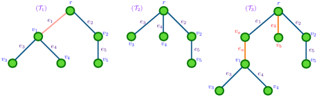
Figure 1: An illustration of transforming a tree structure to another under the lens of edge addition/deletion. Given the binary tree structure ${\mathcal{T}}_{1}$, if we collapse edge $e_{1}$ by merging vertex $v_{1}$ into the root vertex $r$ in ${\mathcal{T}}_{1}$, we obtain the ternary tree structure ${\mathcal{T}}_{2}$. Additionally, in tree ${\mathcal{T}}_{1}$, if we duplicate vertex $v_{1}$ into $\{v_{a},v_{1}\}$, connect these two nodes by edge $e_{a}$; and add the vertex $v_{b}$ with edge $e_{b}$ between $v_{b}$ and root $r$, then we obtain the ternary tree structure ${\mathcal{T}}_{3}$.

Example 3.2 (Edge deletion for tree metric).

Let consider tree ${\mathcal{T}}_{1}$ as in Figure 1 and set $w_{e_{1}}=0$. Tree ${\mathcal{T}}_{2}$ is constructed from ${\mathcal{T}}_{1}$ as in Figure 1. Given two probability measures $\mu=a_{1}\delta_{r}+a_{2}\delta_{v_{1}}+a_{3}\delta_{v_{5}}$ and $\nu=b_{1}\delta_{v_{2}}+b_{2}\delta_{v_{4}}$ in ${\mathcal{T}}_{1}$ (i.e., $a_{1},a_{2},a_{3},b_{1},b_{2}\geq 0;a_{1}+a_{2}+a_{3}=1;b_{1}+b_{2}=1$), their corresponding measures in ${\mathcal{T}}_{2}$ are $\mu_{{\mathcal{T}}_{2}}=(a_{1}+a_{2})\delta_{r}+a_{3}\delta_{v_{5}}$ and $\nu_{{\mathcal{T}}_{2}}=\nu$ respectively. Then, we have ${\mathcal{W}}_{{\mathcal{T}}_{1}}(\mu,\nu)={\mathcal{W}}_{{\mathcal{T}}_{2}}(\mu_{{\mathcal{T}}_{2}},\nu_{{\mathcal{T}}_{2}})$.

Example 3.3 (Edge addition for tree metric).

Let consider tree ${\mathcal{T}}_{1}$ as in Figure 1. Tree ${\mathcal{T}}_{3}$ is constructed from ${\mathcal{T}}_{1}$ as in Figure 1, and we set $w_{e_{a}}=w_{e_{b}}=0$. Given two probability measures $\mu=a_{1}\delta_{v_{1}}+a_{2}\delta_{v_{5}}$ and $\nu=b_{1}\delta_{v_{2}}+b_{2}\delta_{v_{4}}$ in ${\mathcal{T}}_{1}$ (i.e., $a_{1},a_{2},b_{1},b_{2}\geq 0;a_{1}+a_{2}=1;b_{1}+b_{2}=1$), their corresponding measures in ${\mathcal{T}}_{3}$ are $\mu_{{\mathcal{T}}_{3}}=a_{11}\delta_{v_{a}}+a_{12}\delta_{v_{1}}+a_{2}\delta_{v_{5}}$ where $a_{11},a_{12}\geq 0;a_{11}+a_{12}=a_{1}$ and $\nu_{{\mathcal{T}}_{3}}=\nu$ respectively. Then, regardless any split mass ($a_{11},a_{12}$) in $\mu_{{\mathcal{T}}_{3}}$ in ${\mathcal{T}}_{3}$ from original $\mu$ in ${\mathcal{T}}$, we have ${\mathcal{W}}_{{\mathcal{T}}_{1}}(\mu,\nu)={\mathcal{W}}_{{\mathcal{T}}_{3}}(\mu_{{\mathcal{T}}_{3}},\nu_{{\mathcal{T}}_{3}})$.

Therefore, we can add or delete edges with $0$-length on the given tree ${\mathcal{T}}$ without changing the OT distance. More concretely, (i) for edge deletion, we collapse edges with $0$-length in ${\mathcal{T}}$ by merging the two corresponding vertices of those edges together (see Example 3.2); (ii) for edge addition, we duplicate any vertex in ${\mathcal{T}}$ and connect them with $0$-length edge (see Example 3.3). These actions help to transform the given tree structure ${\mathcal{T}}$ into various tree structures, which play the fundamental role to construct uncertainty sets with diverse tree structures. Additionally, we further vary edge lengths of these tree structures to derive our novel uncertainty sets of tree metrics.

The proposed uncertainty sets not only include tree metrics with a variety of tree structures (i.e., all subtree structures of the given tree ${\mathcal{T}}$), but also tree metrics with varying edge lengths. In particular, one can further expand the expressiveness of these sets to cover more diverse tree structures by adding more edges with $0$-length for tree ${\mathcal{T}}$ before varying its edge lengths (e.g., expanding tree ${\mathcal{T}}_{1}$ into tree ${\mathcal{T}}_{3}$ as in Figure 1, and using ${\mathcal{T}}_{3}$ as the given tree), but it comes with a trade-off about the computation of the robust OT.

More precisely, given tree ${\mathcal{T}}=(V,E)$ with nonnegative weights $\{w_{e}\}_{e\in E}$, following Theorem 3.1, it suffices to consider a family of tree metrics for ${\mathcal{T}}$ where these tree structures share the same set of nodes $V$, the same root $r$, and the same set of edges $E$ as in ${\mathcal{T}}$, but their edge lengths (i.e., edge weights) can be varied. To display this dependence on the vector of edge lengths, we will write ${\mathcal{T}}(\hat{w})$ for the tree in this family corresponding to the vector of edge lengths $\hat{w}=(\hat{w}_{e})_{e\in E}\in\mathbb{R}^{|E|}_{+}$. In particular, we consider two approaches on varying edge lengths for the proposed uncertainty sets.

(i) Constraints on individual edge. We consider an uncertainty for each edge length $\hat{w}_{e}$ of edge $e\in E$ in tree ${\mathcal{T}}(\hat{w})$. Specifically, we consider $\hat{w}_{e}$ belongs to some uncertainty interval $w_{e}-\alpha_{e}\leq\hat{w}_{e}\leq w_{e}+\beta_{e}$ around the edge weight $w_{e}$ in tree ${\mathcal{T}}$. In the vector form, this just means that $w-\alpha\leq\hat{w}\leq w+\beta$, with $\alpha,\,\beta\in\mathbb{R}^{|E|}_{+}$ satisfying $\alpha\leq w$ (i.e., edge weights are nonnegative). Thus, $w-\alpha$ and $w+\beta$ are respectively the lower and upper limits of the uncertainty interval for the vector of edge lengths.

(ii) Constraints on set of edges. We consider an uncertainty for all edge lengths of tree ${\mathcal{T}}(\hat{w})$ where the vector of edge lengths $\hat{w}$ is nonnegative (i.e., $\hat{w}\geq 0$), and belongs to an uncertainty closed $\ell_{p}$-ball $\overline{\mathcal{B}}_{p}(w,\lambda)$ centering at $w=(w_{e})_{e\in E}$ and with radius $\lambda>0$. We assume that $1\leq p\leq\infty$ and the uncertainty ball satisfies $\overline{\mathcal{B}}_{p}(w,\lambda)\subset\mathbb{R}^{|E|}_{+}$.

Closed-form expressions. By building upon the proposed uncertainty sets of tree metrics and leveraging tree structure, we derive closed-form expressions for the max-min robust OT, similar to its counterpart standard OT (i.e., TW).

$\bullet$ For constraints on individual edge. Given two vectors $\alpha,\,\beta\in\mathbb{R}^{|E|}_{+}$ satisfying $\alpha\leq w$ (to guarantee the nonnegativeness for edge lengths), we define an uncertainty set for tree ${\mathcal{T}}(\hat{w})$ as follows

$${\mathcal{U}}({\mathcal{T}}\!,\alpha,\beta)\triangleq\left\{\!\hat{\mathcal{T}}={\mathcal{T}}(\hat{w})\mid-\alpha_{e}\leq\hat{w}_{e}-w_{e}\leq\beta_{e},\,\forall e\in E\right\}.$$

The robust OT in Problem (3) can be reformulated as

$$\textsf{RT}_{{\mathcal{U}}}(\mu,\nu)\triangleq\max_{\hat{\mathcal{T}}\in{\mathcal{U}}({\mathcal{T}},\alpha,\beta)}{\mathcal{W}}_{\hat{\mathcal{T}}}(\mu,\nu).$$ (5)

By leveraging the underlying tree structure for OT between measures $\mu$ and $\nu$ with tree metric $d_{\hat{\mathcal{T}}}$, we can further rewrite Problem (5) as

$$\textsf{RT}_{{\mathcal{U}}}(\mu,\nu)=\max_{w-\alpha\leq\hat{w}\leq w+\beta}\sum_{e\in E}\hat{w}_{e}\left|\mu(\gamma_{e})-\nu(\gamma_{e})\right|.$$ (6)

Notice that $\mu(\gamma_{e})$ and $\nu(\gamma_{e})$ only depend on the supports of $\mu$ and $\nu$ (i.e., corresponding nodes in $V$) and on the mass on these supports. In particular, these two terms $\mu(\gamma_{e})$ and $\nu(\gamma_{e})$ are independent of the edge length $\hat{w}_{e}$ on each edge $e\in E$ of tree ${\mathcal{T}}(\hat{w})$. Therefore, we can compute $\textsf{RT}_{{\mathcal{U}}}(\mu,\nu)$ analytically:

$$\textsf{RT}_{{\mathcal{U}}}(\mu,\nu)=\sum_{e\in E}(w_{e}+\beta_{e})\left|\mu(\gamma_{e})-\nu(\gamma_{e})\right|,$$ (7)

where we recall that $w_{e}+\beta_{e}$ is the upper limit of the uncertainty edge weight interval for each edge $e\in E$ in ${\mathcal{U}}({\mathcal{T}}\!,\alpha,\beta)$.

$\bullet$ For constraints on set of edges. Given a radius $\lambda>0$ such that $\overline{\mathcal{B}}_{p}(w,\lambda)\subset\mathbb{R}^{|E|}_{+}$, we define an uncertainty set for tree ${\mathcal{T}}(\hat{w})$ as follows:

$${\mathcal{U}}_{p}({\mathcal{T}},\lambda)\triangleq\left\{\hat{\mathcal{T}}={\mathcal{T}}(\hat{w})\mid\hat{w}\in\overline{\mathcal{B}}_{p}(w,\lambda),\hat{w}\geq 0\right\}.$$

The robust OT corresponding to the uncertainty set ${\mathcal{U}}_{p}({\mathcal{T}},\lambda)$ is

$$\textsf{RT}_{{\mathcal{U}}_{p}}(\mu,\nu)\triangleq\max_{\hat{\mathcal{T}}\in{\mathcal{U}}_{p}({\mathcal{T}},\lambda)}{\mathcal{W}}_{\hat{\mathcal{T}}}(\mu,\nu).$$ (8)

Similarly, we leverage the underlying tree structure for OT between $\mu$ and $\nu$ with tree metric $d_{\hat{\mathcal{T}}}$ to reformulate the definition in (8) as

$$\textsf{RT}_{{\mathcal{U}}_{p}}(\mu,\nu)=\max_{\begin{subarray}{c}\hat{w}\geq 0\\ \hat{w}\in\overline{\mathcal{B}}_{p}(w,\lambda)\end{subarray}}\sum_{e\in E}\hat{w}_{e}\left|\mu(\gamma_{e})-\nu(\gamma_{e})\right|.$$ (9)

By simply leveraging the dual norm, we derive the closed-form expression for $\textsf{RT}_{{\mathcal{U}}_{p}}(\mu,\nu)$ in Problem (9):

Proposition 3.4.

Assume that $1\leq p\leq\infty$. Then,

$$\textsf{RT}_{{\mathcal{U}}_{p}}(\mu,\nu)=\Big{(}\sum_{e\in E}w_{e}\left|\mu(\gamma_{e})-\nu(\gamma_{e})\right|\Big{)}+\lambda\left\lVert h\right\rVert_{p^{\prime}},$$ (10)

where $h\in\mathbb{R}^{|E|}$ is the vector with $h_{e}\triangleq\left|\mu(\gamma_{e})-\nu(\gamma_{e})\right|$ for each edge $e$, and $p^{\prime}$ is the conjugate of $p$. Moreover, a maximizer for Problem (9) is given by $\hat{w}_{e}^{*}=w_{e}+\lambda\|h\|_{p^{\prime}}^{-\frac{p^{\prime}}{p}}h_{e}^{p^{\prime}-1}$ for $1<p<\infty$; $\hat{w}_{e}^{*}=w_{e}+\lambda$ for $p=\infty$; and for $p=1$, let $e^{*}\in E$ be s.t. $\|h\|_{\infty}=h_{e^{*}}>0$, then

$$\hat{w}_{e}^{*}=\left\{\begin{array}[]{lr}\!\!w_{e^{*}}+\lambda\hskip 10.00002pt\mbox{ if }\,e=e^{*},\\ \!\!w_{e}\hskip 33.00008pt\mbox{ otherwise.}\end{array}\right.$$

To our knowledge, among various approaches for the max-min robust OT in the literature, our proposed approach is the first one which yields a closed-form expression for fast computation, and is scalable for large-scale applications.

Connection between two approaches. We next draw a connection between two approaches for the robust OT for measures with noisy tree metric as follows:

Proposition 3.5 (Connection between two approaches).

Assume that $\beta=\lambda\mathbbm{1}$. Then, we have

$$\textsf{RT}_{{\mathcal{U}}({\mathcal{T}},\alpha,\beta)}(\cdot,\cdot)=\textsf{RT}_{{\mathcal{U}}_{\infty}({\mathcal{T}},\lambda)}(\cdot,\cdot).$$ (11)

Computational complexity. From the closed-form expressions for $\textsf{RT}_{{\mathcal{U}}}$ in (7) and for $\textsf{RT}_{{\mathcal{U}}_{p}}$ in (10), the computational complexity of robust OT $\textsf{RT}_{{\mathcal{U}}}$ and $\textsf{RT}_{{\mathcal{U}}_{p}}$ for measures with noisy tree metric is linear to the number of edges in ${\mathcal{T}}$ (i.e., $\mathcal{O}(|E|)$), which is in the same order of computational complexity as the counterpart standard OT for measures with tree metric (i.e., TW) (Ba et al., 2011; Le et al., 2019). Recall that, in general, the max-min robust OT problem is hard and expensive to compute due to its non-convexity and non-smoothness (Paty & Cuturi, 2019; Lin et al., 2020), even for measures supported in $1$-dimensional space (Deshpande et al., 2019).

Improved complexity. Let $\text{supp}(\mu)$ and $\text{supp}(\nu)$ be supports of measures $\mu$ and $\nu$ respectively, and define

$$E_{\mu,\nu}\triangleq\left\{e\in E\mid e\subset[r,z]\mbox{ with $z\in$ }\text{supp}(\mu)\cup\text{supp}(\nu)\right\}.$$

Then, observe that $\mu(\gamma_{e})=\nu(\gamma_{e})=0$ for any edge $e\in E\setminus E_{\mu,\nu}$. Consequently, we can further reduce the computational complexity of the robust OT $\textsf{RT}_{{\mathcal{U}}}$ and $\textsf{RT}_{{\mathcal{U}}_{p}}$ into just $\mathcal{O}(|E_{\mu,\nu}|)$.

Negative definiteness. We next prove that the robust OT for measures with noisy tree metric is negative definite. Therefore, we can derive positive definite kernels built upon the robust OT.

Theorem 3.6 (Negative definiteness).

$\textsf{RT}_{{\mathcal{U}}}$ is negative definite. In addition, $\textsf{RT}_{{\mathcal{U}}_{p}}$ is also negative definite for all $2\leq p\leq\infty$.

Positive definite kernels. From the negative definite results in Theorem 3.6 and by following (Berg et al., 1984, Theorem 3.2.2, pp.74), given $2\leq p\leq\infty$ and $t>0$, we propose positive definite kernels built upon the robust OT for both approaches as follows:

$$k_{\textsf{RT}_{{\mathcal{U}}}}(\mu,\nu)=\exp(-t\textsf{RT}_{{\mathcal{U}}}(\mu,\nu)),$$ (12)

$$k_{\textsf{RT}_{{\mathcal{U}}_{p}}}(\mu,\nu)=\exp(-t\textsf{RT}_{{\mathcal{U}}_{p}}(\mu,\nu)).$$ (13)

To our knowledge, among various existing approaches for the max-min/min-max robust OT, our work is the first provable approach to derive positive definite kernels built upon the robust OT.

Infinite divisibility for the robust OT kernels. We next illustrate the infinite divisibility for the robust OT kernels for measures with noisy tree metric.

Proposition 3.7 (Infinitely divisible kernels).

The kernel $k_{\textsf{RT}_{{\mathcal{U}}}}$ is infinitely divisible. Also, the kernel $k_{\textsf{RT}_{{\mathcal{U}}_{p}}}$ is infinitely divisible for all $2\leq p\leq\infty$.

As for infinitely divisible kernels, one does not need to recompute the Gram matrix of kernels $k_{\textsf{RT}_{{\mathcal{U}}}}$ and $k_{\textsf{RT}_{{\mathcal{U}}_{p}}}$ with $2\leq p\leq\infty$ for each choice of hyperparameter $t$, since it suffices to compute these robust OT kernels for probability measures in the training set once.

Metric property. We end this section by showing that the robust OT is a metric.

Proposition 3.8 (Metric).

$\textsf{RT}_{{\mathcal{U}}}$ is a metric. Also, $\textsf{RT}_{{\mathcal{U}}_{p}}$ is a metric for all $1\leq p\leq\infty$.

4 Related work and discussion

In this section, we discuss related work to the max-min robust OT approach for OT problem for measures with noisy tree metric. We further distinguish it with other lines of research in OT.

One of seminal works in max-min robust OT is the projection robust Wasserstein (Paty & Cuturi, 2019) (i.e., Wasserstein projection pursuit (Niles-Weed & Rigollet, 2022)). This approach considers the maximal possible Wasserstein distance over all possible low dimensional projections. This problem is non-convex and non-smooth, which is hard and expensive to compute (Lin et al., 2020). By leveraging the Riemannian optimization, Lin et al. (2020) derived an efficient algorithmic approach which provides the finite-time guarantee for the computation of the projection robust Wasserstein. Paty & Cuturi (2019) considered its convexified relaxation min-max robust OT, namely subspace robust Wasserstein distance, which provides an upper bound for the projection robust Wasserstein. Alvarez-Melis et al. (2018) proposed the submodular OT to reflect additional structures for OT. Genevay et al. (2018) used min-max robust OT as a loss to improve generative model for images. Dhouib et al. (2020) considered the minimax OT which jointly optimizes the cost matrix and the transportation plan for OT.

Notice that the robust OT approach for OT problem with noisy ground cost is dissimilar to the Wasserstein distributionally robust optimization (Kuhn et al., 2019; Blanchet et al., 2021). Although they may share the min-max formulation, the Wasserstein distributionally robust optimization seeks the best data-driven decision under the most adverse distribution from a Wasserstein ball of a certain radius. Additionally, one should distinguish this robust OT approach for noisy ground cost with the outlier-robust approach for OT where the noise is on input probability measures (Balaji et al., 2020; Mukherjee et al., 2021; Le et al., 2021; Nietert et al., 2022).

Leveraging tree structure to scale up OT problems has been explored for standard OT (Le et al., 2019; Yamada et al., 2022), for OT problem with input measures having different total mass (Sato et al., 2020; Le & Nguyen, 2021), and for Wasserstein barycenter (Takezawa et al., 2022). To our knowledge, our work is the first approach to exploit tree structure over supports to scale up robust OT approach for OT problem with noisy ground cost. Furthermore, notice that max-sliced Wasserstein (Deshpande et al., 2019) is $1$-dimensional OT-based approach for the max-min robust OT. However, there are no fast/efficient algorithmic approaches yet due to its non-convexity. Our approach is based on tree structure which provides more flexibility and degrees of freedoms to capture the topological structure of input probability measures than the 1-dimensional OT-based approach (i.e., choosing a tree rather than a line). Moreover, our novel uncertainty sets of tree metrics play the key role to scale up the computation of robust OT. The uncertainty sets not only includes a diversity of tree structures, but also a variety of edge lengths in an elegant framework following the theoretical guidance in Theorem 3.1.

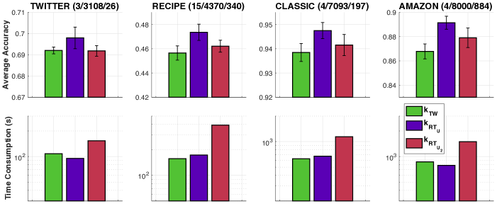
Figure 2: SVM results and time consumption for kernel matrices in document classification. For each dataset, the numbers in the parenthesis are the number of classes; the number of documents; and the maximum number of unique words for each document respectively.

5 Experiments

In this section, we illustrate: (i) fast computation for $\textsf{RT}_{{\mathcal{U}}}$ and $\textsf{RT}_{{\mathcal{U}}_{p}}$, (ii) the robust OT kernels $k_{\textsf{RT}_{{\mathcal{U}}}}$ and $k_{\textsf{RT}_{{\mathcal{U}}_{p}}}$ improve performances of the counterpart standard OT (i.e., tree-Wasserstein) kernel for measures with noisy tree metric, similar to other existing max-min/min-max robust OT in the OT literature.

More concretely, we compare the proposed robust OT kernels $k_{\textsf{RT}_{{\mathcal{U}}}}$ and $k_{\textsf{RT}_{{\mathcal{U}}_{p}}}$ with the counterpart standard OT (i.e., TW) kernel $k_{\textsf{TW}}$, defined as $k_{\textsf{TW}}(\cdot,\cdot)=\exp(-t{\mathcal{W}}_{{\mathcal{T}}}(\cdot,\cdot))$ for a given $t>0$, for measures with a given noisy tree metric under the same settings on several simulations on document classification and topological data analysis (TDA) with SVM.

We emphasize there are various approaches for the simulations on document classification and TDA. However, it is not the goal of our study.

Document classification. We evaluate on $4$ real-world document datasets: TWITTER, RECIPE, CLASSIC, and AMAZON. Their characteristics are listed in Figure 2. We follow the same approach in (Le et al., 2019) to embed words into vectors in $\mathbb{R}^{300}$, and represent each document as a probability measure where its supports are in $\mathbb{R}^{300}$.

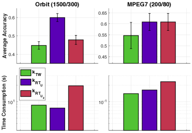
Figure 3: SVM results and time consumption for kernel matrices in TDA. For each dataset, the numbers in the parenthesis are respectively the number of PD; and the maximum number of points in PD.

TDA. We consider orbit recognition on Orbit dataset and object shape recognition on MPEG7 dataset for TDA. We summarize the characteristics of these datasets in Figure 3. We follow the same approach in (Le et al., 2019) to extract persistence diagram (PD) for orbits and object shapes, which are multisets of points in $\mathbb{R}^{2}$, and represent each PD as a probability measure where its supports are in $\mathbb{R}^{2}$.

Noisy tree metric. We apply the clustering-based tree metric sampling method (Le et al., 2019) to obtain a tree metric over supports. We then generate perturbations by deviating each tree edge length by a random nonnegative amount which is less than or equal $\Delta\in\mathbb{R}_{+}$ (i.e., $|w_{e}-w_{e}^{*}|\leq\Delta$) where $w_{e}^{*},w_{e}$ are tree edge lengths on the tree before and after the perturbations respectively. We set $\Delta=0.5$ for document classification (for edge lengths constructed from supports in $\mathbb{R}^{300}$); and set $\Delta=0.05$ for TDA (for edge lengths constructed from supports in $\mathbb{R}^{2}$).

Following Theorem 3.1, the perturbations suffice to cover various tree structures via $0$-length edges (i.e., all subtree structures of the tree before perturbations). Moreover, it is not necessary to add more $0$-length edges before the perturbations for our experiments.

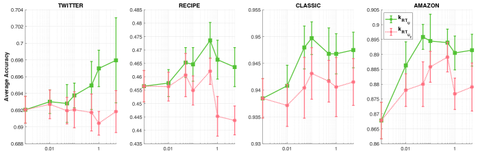
Figure 4: SVM results for document classification w.r.t. the radius $\lambda$.

Experimental setup. We apply kernel SVM for the proposed robust OT kernels $k_{\textsf{RT}_{{\mathcal{U}}}}$ and $k_{\textsf{RT}_{{\mathcal{U}}_{p}}}$ and the counterpart standard OT (i.e., TW) kernel $k_{\textsf{TW}}$ for measures with a given noisy tree metric on document classification and TDA. For $\textsf{RT}_{{\mathcal{U}}}$, we consider $\alpha=\min(\lambda\mathbbm{1},w)$ and $\beta=\lambda\mathbbm{1}$ where minimum operator is element-wise; $\lambda$ is the radius in $\textsf{RT}_{{\mathcal{U}}_{p}}$; and recall that $w$ is a vector of edge lengths of the given tree. We set $p=2$ for the robust OT $\textsf{RT}_{{\mathcal{U}}_{p}}$ (or $\textsf{RT}_{{\mathcal{U}}_{2}}$).

For kernel SVM, we use one-versus-one approach for SVM with multiclass data points. We randomly split each dataset into $70\%/30\%$ for training and test with $10$ repeats. Typically, we use cross validation to choose hyperparameters. For the kernel hyperparameter $t$, we choose $1/t$ from $\{q_{s},2q_{s},5q_{s}\}$ with $s\!=\!10,20,\dotsc,90$, where $q_{s}$ denotes the $s\%$ quantile of a random subset of corresponding distances on training data. For SVM regularization hyperparameter, we choose it from $\left\{0.01,0.1,1,10,100\right\}$. For the radius $\lambda$ in $\textsf{RT}_{{\mathcal{U}}_{2}}$ (also in $\textsf{RT}_{{\mathcal{U}}}$ through the choice of $\beta$), we choose it from $\left\{0.01,0.05,0.1,0.5,1,5\right\}$. All our experiments are run on commodity hardware.

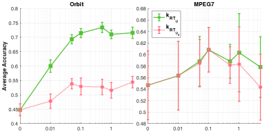
Figure 5: SVM results for TDA w.r.t. the radius $\lambda$.

Empirical results and discussion. Figures 2 and 3 illustrate the performances of SVM for document classification and TDA respectively. The performances of the proposed kernels $k_{\textsf{RT}_{{\mathcal{U}}}}$ and $k_{\textsf{RT}_{{\mathcal{U}}_{2}}}$ compare favorably to those of the counterpart OT kernel $k_{\textsf{TW}}$. Notably, kernel $k_{\textsf{RT}_{{\mathcal{U}}}}$ improves about 15% average accuracy over kernel $k_{\textsf{TW}}$ on Orbit. In addition, kernel $k_{\textsf{RT}_{{\mathcal{U}}}}$ consistently outperforms kernel $k_{\textsf{RT}_{{\mathcal{U}}_{2}}}$, except on MPEG7 where their performances are comparable, which may come from the freedom to constraint over each edge length in ${\mathcal{U}}$ of kernel $k_{\textsf{RT}_{{\mathcal{U}}}}$. Moreover, our results also agree with previous observations on other existing max-min/min-max robust OT where the robust OT approach improves performances of the counterpart standard OT for measures with noisy ground cost. For further discussions, we refer the readers to the supplementary (§C–§D).

Furthermore, the kernels $k_{\textsf{RT}_{{\mathcal{U}}}}$ and $k_{\textsf{RT}_{{\mathcal{U}}_{2}}}$ are fast for computation. They are in the same order as that of the counterpart standard OT (i.e., TW) kernel for measures with noisy tree metric, which agrees with our theoretical analysis in §3 (i.e., linear to the number of edges in the given tree). This is in stark contrast with other existing max-min (or even min-max) robust OT since it is already costly to evaluate the objective function, which is a standard OT for a fixed ground cost, besides the hardness of non-convex and non-smooth optimization problem for max-min robust OT in general.

We next investigate effects of radius $\lambda$ for the robust OT. Recall that $\lambda$ is the radius of the $\ell_{2}$-ball uncertainty for $\textsf{RT}_{{\mathcal{U}}_{2}}$, and we use $\lambda$ for parameter $\beta$ in $\textsf{RT}_{{\mathcal{U}}}$.

Effects of the radius $\lambda$. Figures 4 and 5 illustrate the effects of the radius $\lambda$ on the proposed robust OT kernels on document classification and TDA respectively. Notice that when $\lambda=0$, the max-min robust OT for are equivalent to the counterpart standard OT. We observe that kernel $k_{\textsf{RT}_{{\mathcal{U}}}}$ is less sensitive with the radius $\lambda$ than kernel $k_{\textsf{RT}_{{\mathcal{U}}_{2}}}$. The performances of kernel $k_{\textsf{RT}_{{\mathcal{U}}}}$ gradually increase when the radius $\lambda$ increases, after these performances reach their peaks, they decrease when $\lambda$ increases. The performances of kernel $k_{\textsf{RT}_{{\mathcal{U}}_{2}}}$ also share a similar pattern but more noisy. Therefore, cross validation for the radius $\lambda$ is useful in applications, especially for kernel $k_{\textsf{RT}_{{\mathcal{U}}_{2}}}$ in our simulations.

We place further empirical results with different parameters in the supplementary (§D).

6 Conclusion

In this work, we proposed novel uncertainty sets of tree metrics which not only include metric metrics with varying edge lengths, but also having diverse tree structures in an elegant framework. By building upon these uncertainty sets and leveraging tree structure, we scale up the max-min robust OT approach for OT problem for probability measures with noisy tree metric. Moreover, by exploiting the negative definiteness of the robust OT, we proposed positive definite kernels built upon the robust OT and evaluated them for kernel SVM on document classification and TDA. For future work, extending the problem settings for more general applications (e.g., by leveraging the clustering-based tree metric sampling method), or for more general structures (e.g., graphs) is an interesting direction.

In this supplementary, we give brief reviews about some aspects used in our work, e.g., kernels, tree metric, and optimal transport on for probability measures on a tree in §A. We present detailed proofs for the theoretical results in §B, and give additional discussions about our work in §C. Further experimental results are placed in §D.

Appendix A Brief Reviews

In this section, we briefly review about some aspects used in our work.

A.1 Kernels

We review definitions and theorems about kernels that are used in our work.

Positive Definite Kernels (Berg et al., 1984, pp. 66–67). A kernel function $k:\Omega\times\Omega\rightarrow\mathbb{R}$ is positive definite if for every positive integer $m\geq 2$ and every points $x_{1},x_{2},...,x_{m}\in\Omega$, we have

$$\sum_{i,j=1}^{m}c_{i}c_{j}k(x_{i},x_{j})\geq 0\qquad\forall c_{1},...,c_{m}\in\mathbb{R}.$$

Negative Definite Kernels (Berg et al., 1984, pp. 66–67). A kernel function $k:\Omega\times\Omega\rightarrow\mathbb{R}$ is negative definite if for every integer $m\geq 2$ and every points $x_{1},x_{2},...,x_{m}\in\Omega$, we have

$$\sum_{i,j=1}^{m}c_{i}c_{j}k(x_{i},x_{j})\leq 0,\qquad\quad\forall c_{1},...,c_{m}\in\mathbb{R}\,\,\text{ s.t. }\,\sum_{i=1}^{m}c_{i}=0.$$

Theorem 3.2.2 in (Berg et al., 1984, pp. 74). Let $\kappa$ be a negative definite kernel function. Then, for every $t>0$, the kernel

$$k(x,z)\triangleq\exp{\left(-t\kappa(x,z)\right)}$$

is positive definite.

Definition 2.6 in (Berg et al., 1984, pp. 76). A positive definite kernel $\kappa$ is infinitely divisible if for each $n\in{\mathbb{N}}^{*}$, there exists a positive definite kernel $\kappa_{n}$ such that

$$\kappa=(\kappa_{n})^{n}.$$

Corollary 2.10 in (Berg et al., 1984, pp. 78). Let $\kappa$ be a negative definite kernel function. Then, for $0<t<1$, the kernel

$$k(x,z)\triangleq\left[\kappa(x,z)\right]^{t}$$

is negative definite.

A.2 Tree Metric

We review the definition of tree metric and give detailed references for the clustering-based tree metric sampling method used in our experiments.

Tree metric. A metric $d:\Omega\times\Omega\rightarrow\mathbf{R}$ is a tree metric on $\Omega$ if there exists a tree ${\mathcal{T}}$ with non-negative edge lengths such that all elements of $\Omega$ are contained in its nodes and such that for every $x,z\in\Omega$, we have $d(x,z)$ equals to the length of the path between $x$ and $z$ (Semple & Steel, 2003, §7, pp.145–182). We write $d_{{\mathcal{T}}}$ for the tree metric corresponding to the tree ${\mathcal{T}}$.

Clustering-based tree metric sampling method. The clustering-based tree metric sampling method was proposed by Le et al. (2019) (see their §4). Le et al. (2019) also reviewed the farthest-point clustering in §4.2 in their supplementary, which is the main component used in the clustering-based tree metric sampling method.

A.3 Optimal Transport (OT) for Measures on a Tree

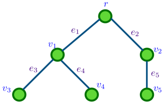
Figure 6: An illustration for a tree with root $r$. The set of nodes $V=\{r,v_{1},v_{2},v_{3},v_{4},v_{5}\}$ and the set of edges $E=\{e_{1},e_{2},e_{3},e_{4},e_{5}\}$. For the edge $e_{1}$, we have $\gamma_{e_{1}}=\{v_{1},v_{3},v_{4}\}$. The path $[r,v_{3}]=\{e_{1},e_{3}\}$.

The $1$-Wasserstein distance ${\mathcal{W}}_{{\mathcal{T}}}$ (with tree metric $d_{{\mathcal{T}}}$ as its ground cost), i.e., tree-Wasserstein (TW), admits a closed-form expression (Ba et al., 2011; Le et al., 2019)

$${\mathcal{W}}_{{\mathcal{T}}}(\mu,\nu)=\sum_{e\in E}w_{e}\left|\mu(\gamma_{e})-\nu(\gamma_{e})\right|,$$ (14)

where $\mu,\,\nu\in{\mathcal{P}}(V)$ and recall that $\gamma_{e}$ is the set of all nodes $x$ such that the path $[r,x]$ contains the edge $e$. An illustration of a set $\gamma_{e}$ is given in Figure 6.

Thanks to formula (14), the computational complexity of TW is linear to the number of edges on tree ${\mathcal{T}}$. Recall that in general the computational complexity of OT is super cubic w.r.t. the number of supports of input measures. We refer the readers to (Le et al., 2019) for further details of TW.

A.4 Persistence Diagrams and Definitions in Topological Data Analysis.

We refer the readers to (Kusano et al., 2017, §2) for a brief review about the mathematical framework for persistence diagrams (e.g., persistence diagrams, filtrations, persistent homology).

Appendix B Proofs

In this section, we give proofs for the theoretical results in the main manuscript.

B.1 Proof for Theorem 3.1

Proof.

Let $E$ and $E^{\prime}$ be the set of edges on trees ${\mathcal{T}}$ and ${\mathcal{T}}^{\prime}$ respectively. Let $e$ be the $0$-length edge which we collapse from tree ${\mathcal{T}}$ to construct tree ${\mathcal{T}}^{\prime}$. Then, we have

$$E=E^{\prime}\cup\{e\}.$$

Moreover, observe that for any edge $\tilde{e}\in E^{\prime}$, $\mu_{{\mathcal{T}}^{\prime}}(\gamma_{\tilde{e}})$ and $\nu_{{\mathcal{T}}^{\prime}}(\gamma_{\tilde{e}})$ in the constructed tree ${\mathcal{T}}^{\prime}$ are the same as their corresponding ones $\mu_{{\mathcal{T}}}(\gamma_{\tilde{e}})$ and $\nu_{{\mathcal{T}}}(\gamma_{\tilde{e}})$ in the original tree ${\mathcal{T}}$ respectively. Therefore, from formula (14) and since $w_{e}=0$, we obtain

$${\mathcal{W}}_{{\mathcal{T}}}(\mu,\nu) =\sum_{\tilde{e}\in E}w_{\tilde{e}}\left|\mu(\gamma_{\tilde{e}})-\nu(\gamma_{\tilde{e}})\right|$$

$$=\Big{(}\sum_{{\tilde{e}}\in E^{\prime}}w_{\tilde{e}}\left|\mu_{{\mathcal{T}}^{\prime}}(\gamma_{\tilde{e}})-\nu_{{\mathcal{T}}^{\prime}}(\gamma_{\tilde{e}})\right|\Big{)}+w_{e}\left|\mu(\gamma_{e})-\nu(\gamma_{e})\right|$$

$$=\sum_{e\in E^{\prime}}w_{e}\left|\mu_{{\mathcal{T}}^{\prime}}(\gamma_{e})-\nu_{{\mathcal{T}}^{\prime}}(\gamma_{e})\right|={\mathcal{W}}_{{\mathcal{T}}^{\prime}}(\mu_{{\mathcal{T}}^{\prime}},\nu_{{\mathcal{T}}^{\prime}}).$$

This completes the proof.

∎

B.2 Proof for Proposition 3.4

Proof.

Recall that $h\in\mathbb{R}^{|E|}$ is given by $h_{e}=\left|\mu(\gamma_{e})-\nu(\gamma_{e})\right|$, and as pointed out right after (6) that it is independent of the edge length $\hat{w}_{e}$ on each edge $e\in E$ in tree ${\mathcal{T}}(\hat{w})$. The conclusion of identity (10) is obvious if $h$ is the zero vector, and hence we only need to consider the case $h\neq 0$.

Let consider the following problem:

$$\widetilde{\textsf{RT}}_{{\mathcal{U}}_{p}}(\mu,\nu)=\max_{\hat{w}\in\overline{\mathcal{B}}_{p}(w,\lambda)}\sum_{e\in E}\hat{w}_{e}\left|\mu(\gamma_{e})-\nu(\gamma_{e})\right|,$$ (15)

which is similar as $\textsf{RT}_{{\mathcal{U}}_{p}}(\mu,\nu)$ in Problem (9), but without the nonnegative constraint on $\hat{w}$ (i.e., $\hat{w}\geq 0$). We will show that the optimal solution $\hat{w}^{*}$ in Problem (15) is nonnegative. Hence, $\widetilde{\textsf{RT}}_{{\mathcal{U}}_{p}}(\mu,\nu)=\textsf{RT}_{{\mathcal{U}}_{p}}(\mu,\nu)$.

Due to the continuity, we have

$$\widetilde{\textsf{RT}}_{{\mathcal{U}}_{p}}(\mu,\nu)=\max_{\hat{w}\in\overline{\mathcal{B}}_{p}(w,\lambda)}\sum_{e\in E}\hat{w}_{e}h_{e}.$$

This can be further expressed as

$$\widetilde{\textsf{RT}}_{{\mathcal{U}}_{p}}(\mu,\nu)=\sum_{e\in E}w_{e}h_{e}+\max_{\hat{w}\in\overline{\mathcal{B}}_{p}(w,\lambda)}\sum_{e\in E}(\hat{w}_{e}-w_{e})h_{e}.$$ (16)

Since $\sum_{e\in E}(\hat{w}_{e}-w_{e})h_{e}\leq\sum_{e\in E}|\hat{w}_{e}-w_{e}|h_{e}\leq\|\hat{w}-w\|_{p}\|h\|_{p^{\prime}},$ we have on one hand that

$$\max_{\hat{w}\in\overline{\mathcal{B}}_{p}(w,\lambda)}\sum_{e\in E}(\hat{w}_{e}-w_{e})h_{e}\leq\lambda\|h\|_{p^{\prime}}.$$ (17)

On the other hand, for the case $1<p<\infty$, by taking

$$\hat{w}_{e}^{*}\triangleq w_{e}+\lambda\|h\|_{p^{\prime}}^{-\frac{p^{\prime}}{p}}h_{e}^{p^{\prime}-1}$$

and as $p^{\prime}=\frac{p}{p-1}$ we see that $\|\hat{w}^{*}-w\|_{p}=\lambda$ and

$$\sum_{e\in E}(\hat{w}_{e}^{*}-w_{e})h_{e} =\lambda\|h\|_{p^{\prime}}^{-\frac{p^{\prime}}{p}}\sum_{e\in E}h_{e}^{p^{\prime}}$$

$$=\lambda\|h\|_{p^{\prime}}^{p^{\prime}(1-\frac{1}{p})}=\lambda\|h\|_{p^{\prime}}.$$

Therefore, we conclude that

$$\max_{\hat{w}\in\overline{\mathcal{B}}_{p}(w,\lambda)}\sum_{e\in E}(\hat{w}_{e}-w_{e})h_{e}=\lambda\|h\|_{p^{\prime}}$$

with $\hat{w}=\hat{w}^{*}$ being a maximizer. Additionally, notice that $w,h\geq 0$, hence, $\hat{w}^{*}\geq 0$. Therefore, together with (16) yields the conclusion of the Proposition for the case $1<p<\infty$.

For the case $p=1$, let $e^{*}\in E$ be such that $\|h\|_{\infty}=h_{e^{*}}>0$. Then, by taking

$$\hat{w}_{e}^{*}\triangleq\left\{\begin{array}[]{lr}\!\!w_{e^{*}}+\lambda\hskip 10.00002pt\mbox{ if }\,e=e^{*},\\ \!\!w_{e}\hskip 33.00008pt\mbox{ otherwise,}\end{array}\right.$$

we see that $\|\hat{w}^{*}-w\|_{1}=\lambda$ and

$$\sum_{e\in E}(\hat{w}_{e}^{*}-w_{e})h_{e} =\lambda h_{e^{*}}=\lambda\|h\|_{\infty}.$$

This and (17) imply that $\max_{\hat{w}\in\overline{\mathcal{B}}_{p}(w,\lambda)}\sum_{e\in E}(\hat{w}_{e}-w_{e})h_{e}=\lambda\|h\|_{\infty}$ with $\hat{w}=\hat{w}^{*}$ being a maximizer, and notice that $\hat{w}^{*}\geq 0$. The conclusion of the Proposition for the case $p=1$ then follows from this and (16).

For the case $p=\infty$, by taking $\hat{w}_{e}^{*}\triangleq w_{e}+\lambda$ for $e\in E$, we see that $\|\hat{w}^{*}-w\|_{\infty}=\lambda$ and

$$\sum_{e\in E}(\hat{w}_{e}^{*}-w_{e})h_{e} =\lambda\sum_{e\in E}h_{e}=\lambda\|h\|_{1}.$$

This and (17) imply that $\max_{\hat{w}\in\overline{\mathcal{B}}_{p}(w,\lambda)}\sum_{e\in E}(\hat{w}_{e}-w_{e})h_{e}=\lambda\|h\|_{1}$ with $\hat{w}=\hat{w}^{*}$ being a maximizer, and further notice that $\hat{w}^{*}\geq 0$. The conclusion of the Proposition for the case $p=\infty$ then follows from this and (16). ∎

B.3 Proof for Proposition 3.5

Proof.

Let define

$$\widetilde{\mathcal{U}}_{p}({\mathcal{T}},\lambda)\triangleq\left\{\hat{\mathcal{T}}={\mathcal{T}}(\hat{w})\mid\hat{w}\in\overline{\mathcal{B}}_{p}(w,\lambda)\right\},$$ (18)

and suppose that $\alpha=\beta=\lambda\mathbbm{1}$, it follows from the definition of the $\ell_{\infty}$-norm that ${\mathcal{U}}({\mathcal{T}},\alpha,\beta)=\widetilde{\mathcal{U}}_{\infty}({\mathcal{T}},\lambda)$. Thus,

$$\textsf{RT}_{{\mathcal{U}}({\mathcal{T}},\alpha,\beta)}(\cdot,\cdot)=\widetilde{\textsf{RT}}_{{\mathcal{U}}_{\infty}({\mathcal{T}},\lambda)}(\cdot,\cdot),$$ (19)

where we recall that $\widetilde{\textsf{RT}}_{{\mathcal{U}}_{\infty}}$ is defined in (15) with $p=\infty$.

Additionally, following the proof for Proposition 3.4, we also have

$$\widetilde{\textsf{RT}}_{{\mathcal{U}}_{\infty}}(\cdot,\cdot)=\textsf{RT}_{{\mathcal{U}}_{\infty}}(\cdot,\cdot).$$ (20)

Hence, we have

$$\textsf{RT}_{{\mathcal{U}}({\mathcal{T}},\alpha,\beta)}(\cdot,\cdot)=\textsf{RT}_{{\mathcal{U}}_{\infty}({\mathcal{T}},\lambda)}(\cdot,\cdot).$$ (21)

Thanks to formula (7) for $\textsf{RT}_{{\mathcal{U}}({\mathcal{T}},\alpha,\beta)}$ which is independent of $\alpha$, we can further drop the condition $\alpha=\lambda\mathbbm{1}$. That is, connection (21) holds true under the only condition $\beta=\lambda\mathbbm{1}$. Thus, the proof is completed.

∎

B.4 Proof for Theorem 3.6

Proof.

We have $(a,b)\in\mathbb{R}\times\mathbb{R}\mapsto(a-b)^{2}$ is negative definite.

Therefore, following (Berg et al., 1984, Corollary 2.10, pp. 78), for $1\leq p\leq 2$, then we have

$$(a,b)\in\mathbb{R}\times\mathbb{R}\mapsto|a-b|^{p}$$

is negative definite.

Thus, for $1\leq p\leq 2$, the mapping function

$$(x,z)\in\mathbb{R}^{d}\times\mathbb{R}^{d}\mapsto\left\lVert x-z\right\rVert_{p}^{p}$$

is negative definite since it is a sum of negative definite functions.

Again, applying (Berg et al., 1984, Corollary 2.10, pp.78), we conclude that

$$(x,z)\in\mathbb{R}^{d}\times\mathbb{R}^{d}\mapsto\left\lVert x-z\right\rVert_{p}$$

is negative definite when $1\leq p\leq 2$.

Moreover, by using the mapping function

$$\mu\mapsto\left([w_{e}+\beta_{e}]\mu(\gamma_{e})\right)_{e\in E}\in\mathbb{R}^{|E|}_{+},$$

and thanks to formula (7), we can reformulate $\textsf{RT}_{{\mathcal{U}}}$ between two probability measures in ${\mathcal{P}}(V)$ in (5) as the $\ell_{1}$ metric between two corresponding mapped vectors in $\mathbb{R}^{|E|}_{+}$. Therefore, $\textsf{RT}_{{\mathcal{U}}}$ is negative definite.

Similarly, due to formula (10) we can also reformulate $\textsf{RT}_{{\mathcal{U}}_{p}}(\mu,\nu)$ for $\mu,\nu\in{\mathcal{P}}(V)$ as a nonnegative weighted sum of $\ell_{1}$ metric (i.e., under the mapping $\mu\mapsto\left(w_{e}\mu(\gamma_{e})\right)_{e\in E}\in\mathbb{R}^{|E|}_{+}$) and $\ell_{p^{\prime}}$ metric (i.e., under the mapping $\mu\mapsto\left(\mu(\gamma_{e})\right)_{e\in E}\in\mathbb{R}^{|E|}_{+}$) of corresponding mapped vectors in $\mathbb{R}^{|E|}_{+}$, where $p^{\prime}$ is the conjugate of $p$. In addition, $1\leq p^{\prime}\leq 2$ when $2\leq p\leq\infty$. Thus, $\textsf{RT}_{{\mathcal{U}}_{p}}$ is also negative definite for $2\leq p\leq\infty$.

Hence, the proof is complete. ∎

B.5 Proof for Proposition 3.7

Proof.

For probability measures $\mu,\,\nu\in{\mathcal{P}}(V)$ and $m\in N^{*}$, we define kernel

$$k_{\textsf{RT}_{{\mathcal{U}}}}^{m}(\mu,\nu)\triangleq\exp\left(-t\frac{\textsf{RT}_{{\mathcal{U}}}(\mu,\nu)}{m}\right).$$

We have $(k_{\textsf{RT}_{{\mathcal{U}}}}^{m})^{m}(\mu,\nu)=k_{\textsf{RT}_{{\mathcal{U}}}}(\mu,\nu)$ and note that $k_{\textsf{RT}_{{\mathcal{U}}}}^{m}$ is a positive definite kernel. Therefore, following (Berg et al., 1984, §3, Definition 2.6, pp.76), kernel $k_{\textsf{RT}_{{\mathcal{U}}}}$ is infinitely divisible.

Similarly, for all $2\leq p\leq\infty$, we define kernel

$$k_{\textsf{RT}_{{\mathcal{U}}_{p}}}^{m}\triangleq\exp\left(-t\frac{\textsf{RT}_{{\mathcal{U}}_{p}}(\mu,\nu)}{m}\right).$$

We have $(k_{\textsf{RT}_{{\mathcal{U}}_{p}}}^{m})^{m}=k_{\textsf{RT}_{{\mathcal{U}}_{p}}}$ and note that $k_{\textsf{RT}_{{\mathcal{U}}_{p}}}^{m}$ is a positive definite kernel. Therefore, following (Berg et al., 1984, §3, Definition 2.6, pp.76), kernel $k_{\textsf{RT}_{{\mathcal{U}}_{p}}}$ is infinitely divisible. Thus, the proof is complete.

∎

B.6 Proof for Proposition 3.8

Proof.

As in the proof for Theorem 3.6, $\textsf{RT}_{{\mathcal{U}}}$ between two probability measures in ${\mathcal{P}}(V)$ can be rewritten as a $\ell_{1}$ metric between two corresponding mapped vectors in $\mathbb{R}^{|E|}_{+}$, i.e., by using the mapping

$$\mu\mapsto\left([w_{e}+\beta_{e}]\mu(\gamma_{e})\right)_{e\in E}\in\mathbb{R}^{|E|}_{+}.$$

Therefore, $\textsf{RT}_{{\mathcal{U}}}$ is a metric.

Similarly, $\textsf{RT}_{{\mathcal{U}}_{p}}$ between two probability measures in ${\mathcal{P}}(V)$ can be recasted as a nonnegative weighted sum of $\ell_{1}$ metric, i.e., by the mapping

$$\mu\mapsto\left(w_{e}\mu(\gamma_{e})\right)_{e\in E}\in\mathbb{R}^{|E|}_{+},$$

and $\ell_{p^{\prime}}$ metric, i.e., by the mapping

$$\mu\mapsto\left(\mu(\gamma_{e})\right)_{e\in E}\in\mathbb{R}^{|E|}_{+}$$

of corresponding mapped vectors in $\mathbb{R}^{|E|}_{+}$, where $p^{\prime}$ is the conjugate of $p$. Thus, $\textsf{RT}_{{\mathcal{U}}_{p}}$ is a metric for all $1\leq p\leq\infty$. Hence, the proof is complete. ∎

Appendix C Further Discussion

C.1 Related Work

We give further discussion to other related works.

For tree-(sliced-)Wasserstein (Le et al., 2019).

Recall that in this work, we consider OT problem for measures with noisy tree metric. In case, one uses the tree-Wasserstein (TW) (Le et al., 2019) for such problem, its performances may be affected due to the noise on the ground cost since TW fundamentally depends on the underlying tree metric structures over supports, which agrees with our empirical observations in Section 5.

$\bullet$ Problem setting. Le et al. (2019) considers the OT problem for measures with tree metric. For applications with given tree metric, one can directly apply the TW for such applications. For applications without given tree metric, Le et al. (2019) proposed to adaptively sample tree metric for supports of input measures, e.g., partition-based tree metric sampling method for supports in low-dimensional space, or clustering-based tree metric sampling method for supports potentially in high-dimensional space. Whereas in our problem, we consider measures with a given noisy tree metric. In other words, we focus on how to deal with the noise on the ground cost, and to reduce this noise affect on performances for OT problem for measures with tree metric, or TW. Although in this work, we consider a simple setting where the tree metric is given, one can leverage the clustering-based tree metric sampling measures to extend it for applications without given tree metric.

$\bullet$ Extension for general applications via tree metric sampling. For applications without given tree metric, but with Euclidean supports, one can apply the clustering-based tree metric sampling method (Le et al., 2019) to obtain a tree metric for such applications. Such sampled tree metric may be noisy, e.g., due to perturbation on supports of input measures, or noisy/adversarial measurement within the clustering-based tree metric sampling method (i.e., clustering algorithm or initialization). Thus, our approach can tackle for such problems in applications.

In our work, to deal with the noise on tree metric for OT problem, we follow the max-min robust OT for measures with noisy tree metric. As illustrated in our experiments in Section 5, the robust OT approach improves performances of the counterpart standard OT when ground metric cost is noisy.

$\bullet$ Potential combination. There is a potential to combine our approach with the approach in (Le et al., 2019) together. For example, when the tree metric space for supports of probability measures is not given, and we can query tree metrics from an oracle, but only receive perturbed/noisy tree metrics. It is an interesting direction for further investigation.

We further note that averaging over TW corresponding to those sampled tree metrics in (Le et al., 2019) has the benefit of reducing clustering/quantization sensitivity problems for the tree metric sampling methods in (Le et al., 2019).

For $1$-Wasserstein approximation with TW (Yamada et al., 2022).

Yamada et al. (2022) considered to use TW as an approximation model for some given (oracle) $1$-Wasserstein distance. In particular, given some supervised triplets $(\mu,\nu,{\mathcal{W}}(\mu,\nu))$ with measures $\mu,\nu$ being supported on high-dimensional vector space $\mathbb{R}^{n}$. The ground cost metric for the observed $1$-Wasserstein is unknown. Yamada et al. (2022) used TW as a model to fit the observed $1$-Wasserstein distances, i.e., estimate tree metric such that ${\mathcal{W}}_{{\mathcal{T}}}(\cdot,\cdot)={\mathcal{W}}(\cdot,\cdot)$. Therefore, the approach in (Yamada et al., 2022) cannot be used in our considered problem due to the following two main reasons:

• (i) we do not have such supervised clean $1$-Wasserstein distance data in our considered problem (i.e., the observed $1$-Wasserstein distance ${\mathcal{W}}(\mu,\nu)$ corresponding with two input probability measures $\mu$ and $\nu$).

• (ii) our considered probability measures are supported in a given tree metric space $({\mathcal{T}},d_{{\mathcal{T}}})$. Moreover, the given tree structure is not necessarily a physical tree in the sense that the set of vertices $V$ is a subset of some high-dimensional vector space $\mathbb{R}^{n}$, and each edge $e$ is the standard line segment in $\mathbb{R}^{n}$ connecting the two end-points of edge $e$. The given tree structure ${\mathcal{T}}$ in our problem can be non-physical, while in (Yamada et al., 2022), input probability measures $\mu,\nu$ are supported on some high-dimensional vector space $\mathbb{R}^{n}$.

C.2 Other Discussions

For kernels on probability measures with OT geometry.

In general, Wasserstein space is not Hilbertian (Peyré & Cuturi, 2019, §8.3), and the standard OT is indefinite. Thus, it is nontrivial to build positive definite kernels upon OT for probability measures.

For kernels on probability measures with OT geometry, besides the tree-(sliced)-Wasserstein kernel (Le et al., 2019), and sliced-Wasserstein kernel (Kolouri et al., 2016; Carrière et al., 2017), to our knowledge, there are only the permanent kernel (Cuturi et al., 2007) and generating function kernel (Cuturi, 2012). However, they are intractable.

For kernels on general measures with potentially different total mass with OT geometry, to our knowledge, there is only the entropy partial transport kernel (Le & Nguyen, 2021).

For subspace robust Wasserstein (Paty & Cuturi, 2019).

In this work, we considered OT problem for probability measures with noisy tree metric. Recall that the subspace robust Wasserstein (SRW) (Paty & Cuturi, 2019) assumes probability measures supported on high-dimensional vector space $\mathbb{R}^{n}$ and seeks the robustness over its vector subspaces (i.e., $\mathbb{R}^{m}$ with $m<n$). Therefore, the SRW distance is not applicable for the considered problem since it is not clear what is the reasonable notion of subspaces of a given tree metric space in our considered problem. Additionally, note that the given tree structure ${\mathcal{T}}$ in our problem is not necessarily physical, i.e., it can be a non-physical tree structure.

Moreover, for measures supported on high-dimensional Euclidean space (e.g., $\mathbb{R}^{300}$), it takes too much time for the computation of subspace robust Wasserstein (SRW), and the SRW does not scale up for large-scale settings (e.g., see Section D.4).

For noise in the document datasets.

In our empirical simulations, we emphasize that our purposes are to compare different transport approaches for probability measures supported on a given tree metric space in the same settings.

Moreover, as discussed in (Sato et al., 2022), the duplication is not the problem for comparing performances in noisy environments. Indeed, in our simulations, we keep the same settings, the only difference is the transport distance. We have no assumptions/requirements that the considered document datasets are clean in our simulations. Therefore, the noise in the considered document datasets are not a problem for our simulations, but provides more diversity for settings in our simulations.

For tree metric.

We applied the clustering-based tree metric sampling method in (Le et al., 2019) to obtain a tree metric and use it as the original given tree metric without perturbation. We emphasize that there is no further processing on that tree metric without perturbation.

For simulations for measures with noisy tree metric, as detailed in Section 5 in the main manuscript, we specifically generate perturbations on each edge length of the original given tree by deviating it by a random nonnegative amount which is less than or equal $\Delta\in\mathbb{R}_{+}$, i.e., $|w_{e}-w_{e}^{*}|\leq\Delta$ where $w_{e}^{*},w_{e}$ are edge lengths on the original tree without perturbation and on the given perturbed tree respectively. We also emphasize that for all edge $e$ in the perturbed tree, we preserve the condition $w_{e}\geq 0$. When there exist edge $e$ with $0$-length, i.e., $w_{e}=0$ in the noisy tree, it can be interpreted that the perturbed tree not only changes its edge lengths, but also its structure (see Theorem 3.1).

Note that, when there is no perturbation on the given tree metric, it is equivalent to $\Delta=0$.

For time consumptions of the robust OT.

As in §3 in the main manuscript, we show that the computational complexity of the max-min robust OT for measures with tree metric is linear to the number of edges in tree ${\mathcal{T}}$ which is in the same order as the counterpart TW, i.e., standard OT with tree metric ground cost. Moreover, in general, the max-min robust OT is hard and expensive to compute due to its non-convexity and non-smoothness, i.e., a maximization problem w.r.t. tree metric with OT as its objective function. This problem remains hard even for supports in $1$-dimensional space (Deshpande et al., 2019). We further note that even with a given optimal ground metric cost, the computational complexity of max-min/min-max robust OT is in the same order as their counterpart standard OT (i.e., their objective function).

As in the experimental results in Section 5, illustrated in Figures 2, and 3, the time consumptions of the robust OT are comparable with the counterpart TW (i.e., OT with tree metric ground cost) for measures with noisy tree metric. The robust OT with the global approach is a little slower than that of others. This is a stark contrast to other approaches for max-min robust OT problem in general. The proposed novel uncertainty sets of tree metrics play an important role for scalability of robust OT for measures with tree metric (e.g., comparing to the $1$-dimensional OT-based approach for max-min robust OT (Deshpande et al., 2019) where there is no efficient/fast algorithmic approach for it yet.)

For performances of the robust OT.

We emphasize that we consider the OT problem for measures with noisy tree metric. The empirical results in Figures 2, and 3 illustrate that the max-min robust OT approach helps to mitigate this issue in applications. When the given tree metric is perturbed, the performances of the proposed kernels $k_{\textsf{RT}_{{\mathcal{U}}}}$ and $k_{\textsf{RT}_{{\mathcal{U}}_{2}}}$ compare favorably to those of the counterpart standard OT (i.e., TW) kernel $k_{\textsf{TW}}$.

Additionally, Figures 7, 8 illustrate further empirical results where the given tree metric is directly obtained from the sampling method without perturbation (or with $\Delta=0$).. The performances of the proposed kernels for the max-min robust OT $k_{\textsf{RT}_{{\mathcal{U}}}}$ and $k_{\textsf{RT}_{{\mathcal{U}}_{2}}}$ are comparable to the counterpart standard OT (i.e., TW) kernel $k_{\textsf{TW}}$. Interestingly, in Orbit dataset, our proposed kernels $k_{\textsf{RT}_{{\mathcal{U}}}}$ and $k_{\textsf{RT}_{{\mathcal{U}}_{2}}}$ improves performances of kernel $k_{\textsf{TW}}$. This may suggest that the given tree ${\mathcal{T}}$ in Orbit dataset might be subjected to noise in our simulations.

Comparing SVM results in Figures 7, 8 for measures with original tree metric (i.e., directly obtained from the sampling method without perturbation, or with $\Delta=0$) and SVM results in Figures 2, and 3 for measures with noisy tree metric (i.e., $\Delta=0.5$), the noise on tree metric did harm performances of TW for all datasets in document classification and TDA. The robust OT approach helps to mitigate the effect of noisy metric for measures in applications.

Remarks.

A concurrent work has recently published in ArXiv (Yamada et al., 2023) where Yamada et al. (2023) leverage the min-max robust variant of tree-Wasserstein for simplicial representation learning by employing self-supervised learning approach based on SimCLR. Empirically, Yamada et al. (2023) also illustrated the advantages of their proposed method over standard SimCLR and cosine-based representation learning.

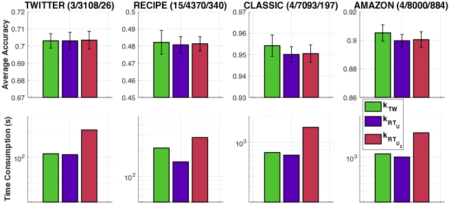
Figure 7: SVM results and time consumption for kernel matrices in document classification when there is no perturbation on the given tree metric (i.e., tree metric obtained from the sampling method without perturbation) (or with $\Delta=0$). For each dataset, the numbers in the parenthesis are the number of classes; the number of documents; and the maximum number of unique words for each document respectively.

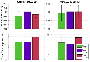
Figure 8: SVM results and time consumption for kernel matrices in TDA when there is no perturbation on the given tree metric (i.e., tree metric obtained from the sampling method without perturbation) (or with $\Delta=0$). For each dataset, the numbers in the parenthesis are respectively the number of PD; and the maximum number of points in PD.

C.3 More Details about Experiments

We describe further details about softwares and datasets.

Softwares.

• For our simulations in TDA, we used DIPHA toolbox to extract persistence diagrams. The DIPHA toolbox is available at https://github.com/DIPHA/dipha.

• For the clustering-based tree metric sampling, we used the MATLAB code at https://github.com/lttam/TreeWasserstein. We directly used this code for clustering-based tree metric sampling without any further processing to obtain the original tree metric without perturbation in our simulations.

Datasets.

• For the document datasets (e.g., TWITTER, RECIPE, CLASSIC, AMAZON), they are available at https://github.com/mkusner/wmd.

• For Orbit dataset, we follow the procedure in Adams et al. (2017) to generate it.

• For MPEG7 dataset, it is available at http://www.imageprocessingplace.com/downloads_V3/root_downloads/image_databases/MPEG7_CE-Shape-1_Part_B.zip. We then extract the $10$-class subset of the dataset as in (Le et al., 2019).

Appendix D Further Experimental Results

In this section, we give further detailed results for our simulations.

D.1 Document Classification

For tree metric without perturbation (i.e., $\Delta=0$).

We give detailed results for robust OT with different value of $\lambda$ in Figures 9, 10, 11, 12, 13, and 14.

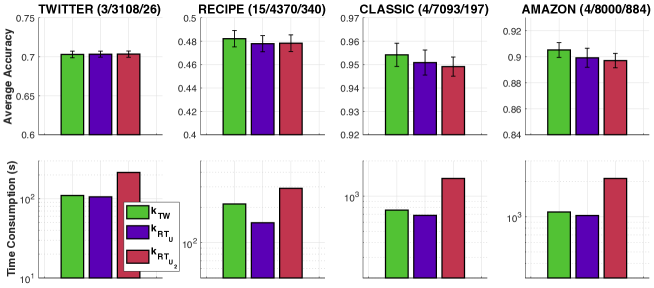
Figure 9: Results on document classification for $\Delta=0$ and $\lambda=0.01$.

Figure 10: Results on document classification for $\Delta=0$ and $\lambda=0.05$.

Figure 11: Results on document classification for $\Delta=0$ and $\lambda=0.1$.

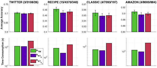
Figure 12: Results on document classification for $\Delta=0$ and $\lambda=0.5$.

Figure 13: Results on document classification for $\Delta=0$ and $\lambda=1$.

Figure 14: Results on document classification for $\Delta=0$ and $\lambda=5$.

For noisy tree metric.

We give detailed results for robust OT with different value of $\lambda$ in Figures 15, 16, 17, 18, 19, and 20 when tree metric is perturbed with $\Delta=0.5$.

Figure 15: Results on document classification for $\Delta=0.5$ and $\lambda=0.01$.

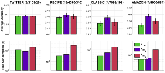
Figure 16: Results on document classification for $\Delta=0.5$ and $\lambda=0.05$.

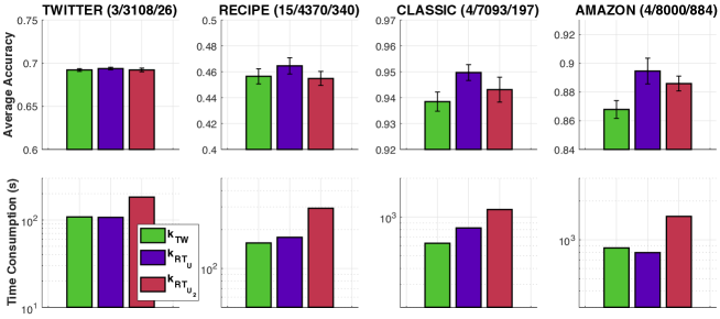
Figure 17: Results on document classification for $\Delta=0.5$ and $\lambda=0.1$.

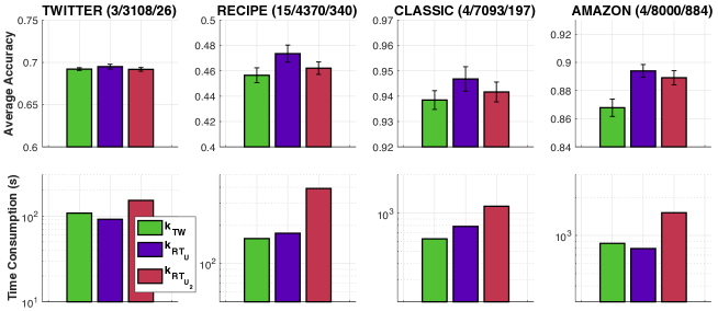
Figure 18: Results on document classification for $\Delta=0.5$ and $\lambda=0.5$.

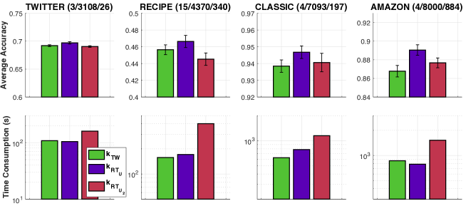
Figure 19: Results on document classification for $\Delta=0.5$ and $\lambda=1$.

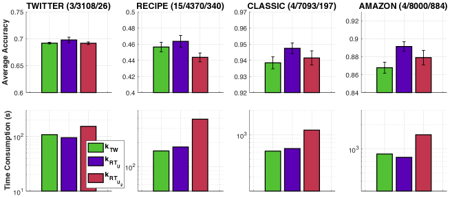
Figure 20: Results on document classification for $\Delta=0.5$ and $\lambda=5$.

D.2 Topological Data Analysis

For tree metric without perturbation (i.e., $\Delta=0$).

We give detailed results for robust OT with different value of $\lambda$ in Figures 21, 22, 23, 24, 25, and 26.

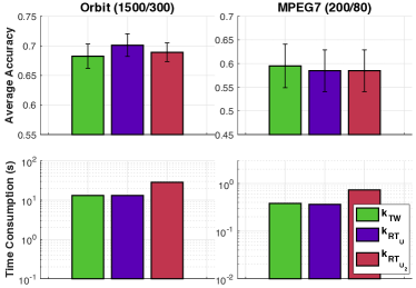
Figure 21: Results on TDA for $\Delta=0$ and $\lambda=0.01$.

Figure 22: Results on TDA for $\Delta=0$ and $\lambda=0.05$.

Figure 23: Results on TDA for $\Delta=0$ and $\lambda=0.1$.

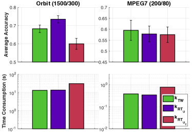
Figure 24: Results on TDA for $\Delta=0$ and $\lambda=0.5$.

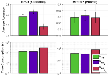
Figure 25: Results on TDA for $\Delta=0$ and $\lambda=1$.

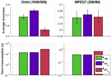
Figure 26: Results on TDA for $\Delta=0$ and $\lambda=5$.

For noisy tree metric.

We give detailed results for robust OT with different value of $\lambda$ in Figures 27, 28, 29, 30, 31, and 32 when tree metric is perturbed with $\Delta=0.05$.

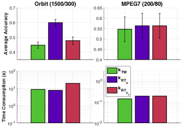
Figure 27: Results on TDA for $\Delta=0.05$ and $\lambda=0.01$.

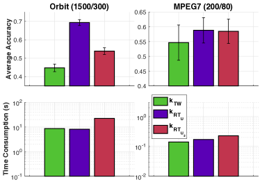
Figure 28: Results on TDA for $\Delta=0.05$ and $\lambda=0.05$.

Figure 29: Results on TDA for $\Delta=0.05$ and $\lambda=0.1$.

Figure 30: Results on TDA for $\Delta=0.05$ and $\lambda=0.5$.

Figure 31: Results on TDA for $\Delta=0.05$ and $\lambda=1$.

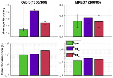
Figure 32: Results on TDA for $\Delta=0.05$ and $\lambda=5$.

D.3 Discussion

Similar to empirical results in the main manuscript, the max-min robust OT for measures with noisy tree metric is fast for computation. Their time consumptions are comparable even to that of the TW (i.e., OT with tree metric ground cost). The max-min robust OT approach helps to mitigate the issue which the given tree metric is perturbed due to noisy or adversarial measurements for OT problem. Hyperparameter $\lambda$ plays an important role for the max-min robust OT for measures with tree metric (e.g., typically chosen via cross-validation).

Table 1: The number of pairs which we compute the distances for both training and test with kernel SVM.

Datasets	#pairs
TWITTER	4394432
RECIPE	8687560
CLASSIC	22890777
AMAZON	29117200
Orbit	1023225
MPEG7	18130

D.4 Further Experiments

Let consider the TWITTER dataset, there are $N=3108$ documents represented as probability measures. Recall that, we randomly split $70\%/30\%$ for training and test with $10$ repeats in our experiments. Thus, for TWITTER dataset, the training set has $N_{tr}=2176$ samples, and the test set has $N_{te}=932$ samples. For the kernel SVM training, the number of pairs which we compute the distances is $(N_{tr}-1)\times\frac{N_{tr}}{2}=2366400$. For the test phase, the number of pairs which we compute the distances is $N_{tr}\times N_{te}=2028032$. Therefore, for $1$ repeat, the number of pairs which we compute the distances for both training and test is totally $4394432$.

When each document in TWITTER dataset is represented by a probability measure supported in the Euclidean space $\mathbb{R}^{300}$, we randomly select $100$ pairs of probability measures to compute the subspace robust Wasserstein (SRW) (Paty & Cuturi, 2019) where the dimension of the subspaces is at most $k_{SRW}=2$. The time consumption of the SRW for each pair is averagely $75.4$ seconds. Therefore, for $1$ repeat, we interpolate that the time consumption for computing the SRW for all pairs in training and test on TWITTER dataset should take about $4$ days averagely, while our robust TW only takes less than 100 seconds for $\textsf{RT}_{{\mathcal{U}}}$, and less than 200 seconds for $\textsf{RT}_{{\mathcal{U}}_{2}}$. The time consumption issue becomes more severe on larger datasets, e.g., AMAZON (with more than $29$M pairs) or CLASSIC (with about $23$M pairs). We summarize the number of pairs which we compute their distances for both training and test for kernel SVM on all datasets in Table 1.

For a bigger picture of empirical results, we extend the SVM results on TWITTER dataset in Figure 2 by adding the SVM results of the corresponding kernel for standard OT with squared Euclidean distance when each document in TWITTER dataset is represented as a measure supported in a high-dimensional Euclidean space $\mathbb{R}^{300}$. We consider two noise levels for the ground metric with squared Euclidean distance: $\frac{L}{2}\Delta$ and $\frac{L}{3}\Delta$ where $L$ is the height of the corresponding tree metric used in the experiments for Figure 2, and we denote them as $k_{\text{OT}}(L\Delta/3)$ and $k_{\text{OT}}(L\Delta/2)$ respectively. As noted in (Le et al., 2019), the standard OT with squared Euclidean ground metric is indefinite and its corresponding kernel is also indefinite. We follow (Le et al., 2019) to add a sufficient regularization on its kernel Gram matrices. Figure 33 illustrates this extended SVM results on TWITTER dataset. Although there are some differences on the experimental setting for $k_{\textsf{TW}}$, $k_{\textsf{RT}_{{\mathcal{U}}}}$, $k_{\textsf{RT}_{{\mathcal{U}}_{2}}}$ with $k_{\text{OT}}(L\Delta/3)$, $k_{\text{OT}}(L\Delta/2)$, Figure 33 illustrates an extended picture for empirical results. The performance of $k_{\text{OT}}$ is improved when the noise level is lower (i.e., $L\Delta/3$), and the indefiniteness may affect the performances of $k_{\text{OT}}$ at some certain. The time consumption of $k_{\text{OT}}$ is slower than other approaches since the time complexity of standard OT with squared Euclidean ground metric is super cubic. Our results also agree with empirical observations in (Le et al., 2019).

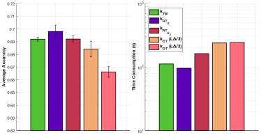
Figure 33: Extended SVM results on TWITTER dataset.

References

- Adams et al. (2017) Adams, H., Emerson, T., Kirby, M., Neville, R., Peterson, C., Shipman, P., Chepushtanova, S., Hanson, E., Motta, F., and Ziegelmeier, L. Persistence images: A stable vector representation of persistent homology. Journal of Machine Learning Research, 18(1):218–252, 2017.
- Altschuler et al. (2021) Altschuler, J. M., Chewi, S., Gerber, P., and Stromme, A. J. Averaging on the Bures-Wasserstein manifold: Dimension-free convergence of gradient descent. Advances in Neural Information Processing Systems, 2021.
- Alvarez-Melis et al. (2018) Alvarez-Melis, D., Jaakkola, T., and Jegelka, S. Structured optimal transport. In International Conference on Artificial Intelligence and Statistics, pp. 1771–1780. PMLR, 2018.
- Ba et al. (2011) Ba, K. D., Nguyen, H. L., Nguyen, H. N., and Rubinfeld, R. Sublinear time algorithms for earth mover’s distance. Theory of Computing Systems, 48:428–442, 2011.
- Balaji et al. (2020) Balaji, Y., Chellappa, R., and Feizi, S. Robust optimal transport with applications in generative modeling and domain adaptation. Advances in Neural Information Processing Systems, 33:12934–12944, 2020.
- Ben-Tal et al. (2009) Ben-Tal, A., El Ghaoui, L., and Nemirovski, A. Robust optimization, volume 28. Princeton university press, 2009.
- Berg et al. (1984) Berg, C., Christensen, J. P. R., and Ressel, P. (eds.). Harmonic analysis on semigroups. Springer-Verglag, New York, 1984.
- Bertsimas et al. (2011) Bertsimas, D., Brown, D. B., and Caramanis, C. Theory and applications of robust optimization. SIAM review, 53(3):464–501, 2011.
- Blanchet et al. (2021) Blanchet, J., Murthy, K., and Nguyen, V. A. Statistical analysis of Wasserstein distributionally robust estimators. In Tutorials in Operations Research: Emerging Optimization Methods and Modeling Techniques with Applications, pp. 227–254. INFORMS, 2021.
- Bunne et al. (2019) Bunne, C., Alvarez-Melis, D., Krause, A., and Jegelka, S. Learning generative models across incomparable spaces. In International Conference on Machine Learning (ICML), volume 97, 2019.
- Bunne et al. (2022) Bunne, C., Papaxanthos, L., Krause, A., and Cuturi, M. Proximal optimal transport modeling of population dynamics. In International Conference on Artificial Intelligence and Statistics, pp. 6511–6528. PMLR, 2022.
- Carrière et al. (2017) Carrière, M., Cuturi, M., and Oudot, S. Sliced Wasserstein kernel for persistence diagrams. In International conference on machine learning, pp. 1–10, 2017.
- Cuturi (2012) Cuturi, M. Positivity and transportation. arXiv preprint arXiv:1209.2655, 2012.
- Cuturi et al. (2007) Cuturi, M., Vert, J.-P., Birkenes, O., and Matsui, T. A kernel for time series based on global alignments. In 2007 IEEE International Conference on Acoustics, Speech and Signal Processing-ICASSP’07, volume 2, pp. II–413. IEEE, 2007.
- Deshpande et al. (2019) Deshpande, I., Hu, Y.-T., Sun, R., Pyrros, A., Siddiqui, N., Koyejo, S., Zhao, Z., Forsyth, D., and Schwing, A. G. Max-sliced Wasserstein distance and its use for GANs. In Proceedings of the IEEE/CVF Conference on Computer Vision and Pattern Recognition, pp. 10648–10656, 2019.
- Dhouib et al. (2020) Dhouib, S., Redko, I., Kerdoncuff, T., Emonet, R., and Sebban, M. A swiss army knife for minimax optimal transport. In International Conference on Machine Learning, pp. 2504–2513. PMLR, 2020.
- El Ghaoui & Lebret (1997) El Ghaoui, L. and Lebret, H. Robust solutions to least-squares problems with uncertain data. SIAM Journal on matrix analysis and applications, 18(4):1035–1064, 1997.
- Fan et al. (2022) Fan, J., Haasler, I., Karlsson, J., and Chen, Y. On the complexity of the optimal transport problem with graph-structured cost. In International Conference on Artificial Intelligence and Statistics, pp. 9147–9165. PMLR, 2022.
- Fatras et al. (2021) Fatras, K., Séjourné, T., Flamary, R., and Courty, N. Unbalanced minibatch optimal transport; applications to domain adaptation. In International Conference on Machine Learning, pp. 3186–3197. PMLR, 2021.
- Genevay et al. (2018) Genevay, A., Peyre, G., and Cuturi, M. Learning generative models with Sinkhorn divergences. In Proceedings of the Twenty-First International Conference on Artificial Intelligence and Statistics, pp. 1608–1617, 2018.
- Janati et al. (2020) Janati, H., Muzellec, B., Peyré, G., and Cuturi, M. Entropic optimal transport between (unbalanced) Gaussian measures has a closed form. In Advances in neural information processing systems, 2020.
- Keel et al. (1988) Keel, L. H., Bhattacharyya, S., and Howze, J. W. Robust control with structure perturbations. IEEE Transactions on Automatic Control, 33(1):68–78, 1988.
- Kolouri et al. (2016) Kolouri, S., Zou, Y., and Rohde, G. K. Sliced wasserstein kernels for probability distributions. In Proceedings of the IEEE Conference on Computer Vision and Pattern Recognition, pp. 5258–5267, 2016.
- Kuhn et al. (2019) Kuhn, D., Esfahani, P. M., Nguyen, V. A., and Shafieezadeh-Abadeh, S. Wasserstein distributionally robust optimization: Theory and applications in machine learning. In Operations research & management science in the age of analytics, pp. 130–166. Informs, 2019.
- Kusano et al. (2017) Kusano, G., Fukumizu, K., and Hiraoka, Y. Kernel method for persistence diagrams via kernel embedding and weight factor. The Journal of Machine Learning Research, 18(1):6947–6987, 2017.
- Lavenant et al. (2018) Lavenant, H., Claici, S., Chien, E., and Solomon, J. Dynamical optimal transport on discrete surfaces. In SIGGRAPH Asia 2018 Technical Papers, pp. 250. ACM, 2018.
- Le et al. (2021) Le, K., Nguyen, H., Nguyen, Q. M., Pham, T., Bui, H., and Ho, N. On robust optimal transport: Computational complexity and barycenter computation. Advances in Neural Information Processing Systems, 34:21947–21959, 2021.
- Le & Nguyen (2021) Le, T. and Nguyen, T. Entropy partial transport with tree metrics: Theory and practice. In Proceedings of The 24th International Conference on Artificial Intelligence and Statistics (AISTATS), volume 130 of Proceedings of Machine Learning Research, pp. 3835–3843. PMLR, 2021.
- Le et al. (2019) Le, T., Yamada, M., Fukumizu, K., and Cuturi, M. Tree-sliced variants of Wasserstein distances. In Advances in neural information processing systems, pp. 12283–12294, 2019.
- Lin et al. (2020) Lin, T., Fan, C., Ho, N., Cuturi, M., and Jordan, M. Projection robust Wasserstein distance and riemannian optimization. Advances in neural information processing systems, 33:9383–9397, 2020.
- Liu et al. (2022) Liu, L., Pal, S., and Harchaoui, Z. Entropy regularized optimal transport independence criterion. In International Conference on Artificial Intelligence and Statistics, pp. 11247–11279. PMLR, 2022.
- Mena & Niles-Weed (2019) Mena, G. and Niles-Weed, J. Statistical bounds for entropic optimal transport: sample complexity and the central limit theorem. In Advances in Neural Information Processing Systems, pp. 4541–4551, 2019.
- Morimoto & Doya (2001) Morimoto, J. and Doya, K. Robust reinforcement learning. Advances in neural information processing systems, pp. 1061–1067, 2001.
- Mukherjee et al. (2021) Mukherjee, D., Guha, A., Solomon, J. M., Sun, Y., and Yurochkin, M. Outlier-robust optimal transport. In International Conference on Machine Learning, pp. 7850–7860. PMLR, 2021.
- Muzellec et al. (2020) Muzellec, B., Josse, J., Boyer, C., and Cuturi, M. Missing data imputation using optimal transport. In International Conference on Machine Learning, pp. 7130–7140. PMLR, 2020.
- Nadjahi et al. (2019) Nadjahi, K., Durmus, A., Simsekli, U., and Badeau, R. Asymptotic guarantees for learning generative models with the sliced-Wasserstein distance. In Advances in Neural Information Processing Systems, pp. 250–260, 2019.
- Nguyen et al. (2022) Nguyen, T. D., Trippe, B. L., and Broderick, T. Many processors, little time: MCMC for partitions via optimal transport couplings. In International Conference on Artificial Intelligence and Statistics, pp. 3483–3514. PMLR, 2022.
- Nietert et al. (2022) Nietert, S., Goldfeld, Z., and Cummings, R. Outlier-robust optimal transport: Duality, structure, and statistical analysis. In International Conference on Artificial Intelligence and Statistics, pp. 11691–11719. PMLR, 2022.
- Niles-Weed & Rigollet (2022) Niles-Weed, J. and Rigollet, P. Estimation of Wasserstein distances in the spiked transport model. Bernoulli, 28(4):2663–2688, 2022.
- Panaganti et al. (2022) Panaganti, K., Xu, Z., Kalathil, D., and Ghavamzadeh, M. Robust reinforcement learning using offline data. In Advances in Neural Information Processing Systems, volume 35, pp. 32211–32224, 2022.
- Paty & Cuturi (2019) Paty, F.-P. and Cuturi, M. Subspace robust Wasserstein distances. In Proceedings of the 36th International Conference on Machine Learning, pp. 5072–5081, 2019.
- Paty et al. (2020) Paty, F.-P., d’Aspremont, A., and Cuturi, M. Regularity as regularization: Smooth and strongly convex Brenier potentials in optimal transport. In International Conference on Artificial Intelligence and Statistics, pp. 1222–1232. PMLR, 2020.
- Peyré & Cuturi (2019) Peyré, G. and Cuturi, M. Computational optimal transport. Foundations and Trends® in Machine Learning, 11(5-6):355–607, 2019.
- Rabin et al. (2011) Rabin, J., Peyré, G., Delon, J., and Bernot, M. Wasserstein barycenter and its application to texture mixing. In International Conference on Scale Space and Variational Methods in Computer Vision, pp. 435–446, 2011.
- Sato et al. (2020) Sato, R., Yamada, M., and Kashima, H. Fast unbalanced optimal transport on tree. In Advances in neural information processing systems, 2020.
- Sato et al. (2022) Sato, R., Yamada, M., and Kashima, H. Re-evaluating word mover’s distance. In International Conference on Machine Learning, pp. 19231–19249, 2022.
- Scetbon et al. (2021) Scetbon, M., Cuturi, M., and Peyré, G. Low-rank Sinkhorn factorization. International Conference on Machine Learning (ICML), 2021.
- Semple & Steel (2003) Semple, C. and Steel, M. Phylogenetics. Oxford Lecture Series in Mathematics and its Applications, 2003.
- Si et al. (2021) Si, N., Murthy, K., Blanchet, J., and Nguyen, V. A. Testing group fairness via optimal transport projections. International Conference on Machine Learning, 2021.
- Solomon et al. (2015) Solomon, J., De Goes, F., Peyré, G., Cuturi, M., Butscher, A., Nguyen, A., Du, T., and Guibas, L. Convolutional Wasserstein distances: Efficient optimal transportation on geometric domains. ACM Transactions on Graphics (TOG), 34(4):66, 2015.
- Tai (1979) Tai, K.-C. The tree-to-tree correction problem. Journal of the ACM, 26(3):422–433, 1979.
- Takezawa et al. (2022) Takezawa, Y., Sato, R., Kozareva, Z., Ravi, S., and Yamada, M. Fixed support tree-sliced Wasserstein barycenter. In Proceedings of The 25th International Conference on Artificial Intelligence and Statistics, volume 151, pp. 1120–1137. PMLR, 2022.
- Titouan et al. (2019) Titouan, V., Courty, N., Tavenard, R., and Flamary, R. Optimal transport for structured data with application on graphs. In International Conference on Machine Learning, pp. 6275–6284. PMLR, 2019.
- Wang et al. (2022) Wang, J., Gao, R., and Xie, Y. Two-sample test with kernel projected Wasserstein distance. In Proceedings of The 25th International Conference on Artificial Intelligence and Statistics, volume 151, pp. 8022–8055. PMLR, 2022.
- Weed & Berthet (2019) Weed, J. and Berthet, Q. Estimation of smooth densities in Wasserstein distance. In Proceedings of the Thirty-Second Conference on Learning Theory, volume 99, pp. 3118–3119, 2019.
- Xu et al. (2008) Xu, H., Caramanis, C., and Mannor, S. Robust regression and lasso. Advances in neural information processing systems, 21, 2008.
- Xu et al. (2009) Xu, H., Caramanis, C., and Mannor, S. Robustness and regularization of support vector machines. Journal of machine learning research, 10(7), 2009.
- Yamada et al. (2022) Yamada, M., Takezawa, Y., Sato, R., Bao, H., Kozareva, Z., and Ravi, S. Approximating 1-Wasserstein distance with trees. Transactions on Machine Learning Research, 2022. ISSN 2835-8856.
- Yamada et al. (2023) Yamada, M., Takezawa, Y., Houry, G., Dusterwald, K. M., Sulem, D., Zhao, H., and Tsai, Y.-H. H. An empirical study of simplicial representation learning with wasserstein distance. arXiv preprint arXiv:2310.10143, 2023.