Be Bayesian by Attachments to Catch More Uncertainty

Abstract

Bayesian Neural Networks (BNNs) have become one of the promising approaches for uncertainty estimation due to the solid theorical foundations. However, the performance of BNNs is affected by the ability of catching uncertainty. Instead of only seeking the distribution of neural network weights by in-distribution (ID) data, in this paper, we propose a new Bayesian Neural Network with an Attached structure (ABNN) to catch more uncertainty from out-of-distribution (OOD) data. We first construct a mathematical description for the uncertainty of OOD data according to the prior distribution, and then develop an attached Bayesian structure to integrate the uncertainty of OOD data into the backbone network. ABNN is composed of an expectation module and several distribution modules. The expectation module is a backbone deep network which focuses on the original task, and the distribution modules are mini Bayesian structures which serve as attachments of the backbone. In particular, the distribution modules aim at extracting the uncertainty from both ID and OOD data. We further provide theoretical analysis for the convergence of ABNN, and experimentally validate its superiority by comparing with some state-of-the-art uncertainty estimation methods Code will be made available.

I Introduction

Deep Neural Networks (DNNs) have gained widespread recognition as highly effective predictive models [1, 2, 3]. However, only remarkable predictive performance may not satisfy all real-life demands. In some safety-critical scenarios, uncertainty estimation poses a significant challenge. [4, 5, 6, 7]. Recent studies have raised concerns about the reliability of DNNs, as they tend to make overconfident predictions [8, 9]. Moreover, when a DNN is presented with out-of-distribution (OOD) samples that significantly differ from the training inputs, it may provide confident but meaningless predictions, which can lead to issues [10, 9]. Therefore, uncertainty estimation remains a challenge for DNNs.

Recently, Bayesian Neural Networks (BNNs) have shown promising performance for uncertainty estimation [11, 12]. BNNs take model parameters as random variables with prior distributions and learn their posterior distributions given data. At test time, BNNs provide random variables with specific distributions as their predictions. There are three major approaches to learn posterior distributions: Markov chain Monte Carlo [13, 14], Laplacian approximation [15, 16] and variational inference [11, 17]. Variational inference, i.e. approximating the true posterior distributions with some simple distributions, is a popular approach [18]. For example, Blundell et al. [11] proposed a backpropagation-compatible algorithm for variational BNN training. Shridhar et al. [19] introduced variational Bayesian inference into Convolution Neural Networks. Kristiadi et al. [20] found it sufficient to build a ReLU network with only a single Bayesian layer.

However, most BNNs only catch uncertainty from in-distribution (ID) training data, which may limit their power [21, 22]. The uncertainty quantification ability of BNNs comes from their posteriors of parameters given data. Since OOD data are usually incomplete (unlabeled or even odd to be labeled), it’s unclear what the true posteriors given OOD data are, let alone estimation. Therefore, it’s a challenge to incorporate OOD data into Bayesian inference. Consequently, sometimes BNNs perform worse than frequentist methods, especially in OOD detection task [23, 22, 24].

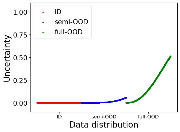
(a) BBP

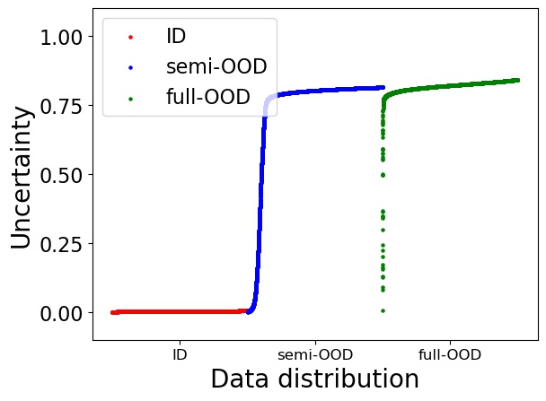
(b) SDE-Net

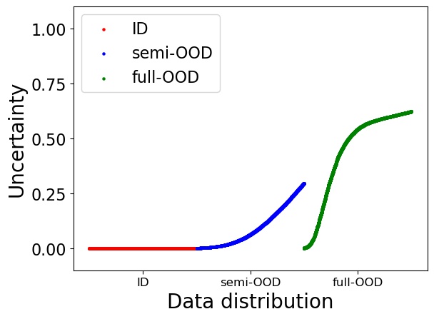
(c) ABNN

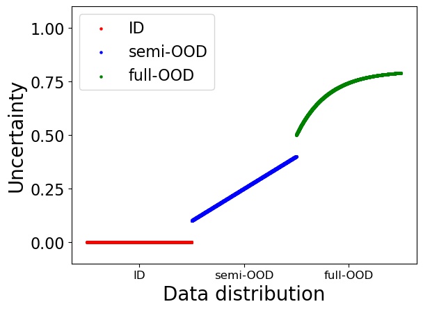
(d) Ideal

Figure 1: Visualization of uncertainty for BBP [11], SDE-Net [25] and ABNN. The horizontal axis is the index of predictions ordered by uncertainty on each dataset, and the longitudinal axis is uncertainty. An ideal estimate should increase gradually as the input becomes more OOD, while still being separable on different datasets. Please refer to Section IV-A for more details.

OOD training has been well studied for OOD detection, and researchers find that using auxiliary outlier data can bring significant improvements [24, 23]. For example, Outlier Exposure (OE) [24] is a simple but effective method that uniformly labels OOD data for classification. Many variants based on OE have been proposed, and they achieved the state-of-the-art performance [23, 26, 27]. However, OE implicitly assumes that all OOD data have the same uncertainty by labeling them in the same way. This is an advantage in OOD detection, but it violates the principle of uncertainty estimation. Assigning the same uncertainty to all OOD data may result in misjudgments of many valuable predictions. The uncertainty should increase continuously as inputs become more dissimilar from ID data. We show how different methods handle uncertainty in Figure 1. Furthermore, directly adapting OE to BNNs is not appropriate, since the posteriors would be questionable given that the pseudo labels for OOD data differ greatly from the true labels.

In this paper, a new Bayesian Neural Network with an Attachment structure (ABNN) is proposed to catch more uncertainty from out-of-distribution data. First, we establish mathematical descriptions for the uncertainty of OOD data based on prior distributions and subdivide OOD data into semi-OOD and full-OOD data. Then, we explore the relationship between uncertainty and parameter variance, and we propose an adversarial strategy to incorporate OOD uncertainty into ID uncertainty. Meanwhile, we develop an attachment structure to mitigate the adverse effect of OOD training on the backbone network. ABNN consists of two modules: an expectation module and several distribution modules. The expectation module focuses on the primary task of the neural network, which is similar to the expectation of a traditional BNN. Distribution modules are mini Bayesian structures aiming to catch the uncertainty from both ID data and OOD data. The structure of distribution modules can be much simpler than the expectation module, because researchers indicate that just a few Bayesian layers are enough to catch uncertainty [20, 28]. Therefore, we design distribution modules to be mini-sized, which seem like attachments of the expectation module.

To summarize, our contributions are:

• We propose a new variational inference BNN framework to catch additional uncertainty from OOD data.

• We refine the definitions for OOD data, propose a new training strategy for OOD data and prove its convergence.

• We design a general attachment structure to maintain the backbone’s predictive power while equipping it with uncertainty estimation ability.

• Empirical studies show ABNN’s superiority over traditional BNNs.

II Mathematical Description

In this section, we will present some necessary definitions and properties. For easy understanding, we only give discussions on balanced classification tasks and take MNIST [29] for example. The definitions and properties can be easily extended to other situations.

II-A Segmentation of ID and OOD data

We first segment the whole data space $\mathcal{D}$ into subspaces $\mathcal{D}_{\rm{ID}}$,$\mathcal{D}_{\rm{semiOOD}}$ and $\mathcal{D}_{\rm{fullOOD}}$ to examine the labels of OOD samples. The segmentation is given by judging whether a sample is directly, or weakly, or not related to some distributions, corresponding to low, middle, and high uncertainty. Our definitions are derived from Liang et al. [30]

Definition 1 ($\mathcal{D}_{\rm{ID}}$).

Let $X$ denote the input, $X\in\mathcal{D}$. $\{f(X,\theta):\theta\in\Theta\}$ is a family of density functions on $\mathcal{D}$, $\theta$ is the parameter, $\Theta$ denotes all the possible parameters that could generate samples in $\mathcal{D}$. Given a subset $\Theta_{0}\subset\Theta$, we define $\mathcal{D}_{\rm{ID}}:=\{X\in\mathcal{D}:\exists\theta\in\Theta_{0},X=\int_{\mathcal{D}}uf(u,\theta)\,du\}$ as in-distribution data space.

For example, in MNIST digits classification, $\mathcal{D}$ is the collection of all possible $28\times 28$ images and $\mathcal{D}_{\rm{ID}}$ is MNIST. If we consider each digit as a sample from a distribution, then $\{f(X,\theta):\theta\in\Theta\}$ is the collection of all the distributions with digits as their expectations. Since MNIST consists of digits with distinctive styles, the density functions of MNIST should be a subset of $\{f(X,\theta):\theta\in\Theta\}$, that is $\{f(X,\theta):\theta\in\Theta_{0}\subset\Theta\}$.

Definition 2 ($\mathcal{D}_{\rm{semiOOD}}$).

Following Definition 1, $\mathcal{D}_{\rm{semiOOD}}:=\{X:\exists\theta\in\Theta\setminus\Theta_{0},X=\int_{\mathcal{D}}uf(u,\theta)\,du\}$.

Definition 3 ($\mathcal{D}_{\rm{fullOOD}}$).

Following Definition 2, $\mathcal{D}_{\rm{fullOOD}}:=\mathcal{D}\setminus(\mathcal{D}_{\rm{ID}}\cup\mathcal{D}_{\rm{semiOOD}})$.

In MNIST digits classification, the collection of all digit images that do not belong to MNIST is $\mathcal{D}_{\rm{semiOOD}}$. They share similar distributions with ID data but have different styles. For example, SVHN [31] is a subset of $\mathcal{D}_{\rm{semiOOD}}$. $\mathcal{D}_{\rm{fullOOD}}$ is all the $28\times 28$ images that are not digits. Note that the labels of OOD data are inaccessible.

II-B Data Distribution

After the segmentation, it becomes possible to select specific distributions to represent ID, semi-OOD, or full-OOD data. Before segmentation, there exists a global prior distribution $p(X)$ for all data, but it’s inaccessible. However, after segmentation, we can define conditional distributions on $\mathcal{D}_{\rm{ID}}$ and $\mathcal{D}_{\rm{semiOOD}}$ based on the constraint of $f(X,\theta)$.

Definition 4 ($p(X|\theta,\mathcal{D}_{\rm{ID}})$).

If $\exists\delta>0$, $\exists\theta_{1},\theta_{2},...,\theta_{K}\in\Theta_{0}$, s.t. $\forall X\in\mathcal{D}_{\rm{ID}}$, $\exists i\in\{1,2,...,K\},\forall j\neq i$ and $j\in\{1,2,...,K\},f(X,\theta_{i})>f(X,\theta_{j})+\delta$. Then we call

$$G(f(X,\theta_{i}))=\left\{\begin{aligned} &f(X,\theta_{i})+\frac{\int_{\mathcal{D}\setminus\mathcal{D}_{\rm{ID}}}f(u,\theta_{i})\,du}{\int_{\mathcal{D}_{\rm{ID}}}1\,du},X\in\mathcal{D}_{\rm{ID}}\\ &0,X\in\mathcal{D}\setminus\mathcal{D}_{\rm{ID}}\end{aligned}\right.$$ (1)

The density function of $X$ given that $X\in\mathcal{D}_{\rm{ID}}$ and belongs to $i_{th}$ class. Denote the prior distribution as $p(X|\theta_{i},\mathcal{D}_{\rm{ID}})$.

We establish this definition based on a common assumption: In classification tasks, each class corresponds to a specific distribution, and the process of classifying a sample is to find the most probable distribution that this sample originates from [32, 33]. For easy notation, we continue to refer to the prior distributions by $f$. If the class of $X$ is not specified, we can calculate its prior distribution by formula $p(X|\mathcal{D}_{\rm{ID}})=\sum_{i=1}^{K}p(\theta_{i})p(X|\theta_{i},\mathcal{D}_{\rm{ID}})$. Meanwhile, we assume that $\theta=\theta_{i}$ corresponds to that $X$ belongs to the $\rm{i_{th}}$ class.

On $\mathcal{D}_{\rm{fullOOD}}$, no data can be represented by $f(X,\theta)$. In other words, $X$ is independent of $\theta$. Following the Bayesian school, $X$ on $\mathcal{D}_{\rm{fullOOD}}$ has the same distribution as their prior distribution, even though the precise formula for this distribution is unknown.

Definition 5 ($p(X|\theta,\mathcal{D}_{\rm{fullOOD}})$).

$p(X|\theta_{i},\mathcal{D}_{\rm{fullOOD}}):=p(X|\mathcal{D}_{\rm{fullOOD}})$ is called the prior distribution of X given that $X\in\mathcal{D}_{\rm{fullOOD}}$ and belongs to $i_{th}$ class. $p(X|\mathcal{D}_{\rm{fullOOD}})$ can be calculated by Bayesian formula: $p(X|\mathcal{D}_{\rm{fullOOD}})=\frac{P(\mathcal{D}_{\rm{fullOOD}}|X)p(X)}{P(\mathcal{D}_{\rm{fullOOD}})}=\mathbb{I}_{X\in\mathcal{D}_{\rm{fullOOD}}}\frac{m(\mathcal{D})}{m(\mathcal{D}_{\rm{fullOOD}})}p(X)$, $\mathbb{I}_{(\cdot)}$ is the indicator function, $m(\cdot)$ is a measure.

On $\mathcal{D}_{\rm{semiOOD}}$, we can define prior distributions similarly as Definition 4. However, we believe that $\theta$ can still be constrained on $\{\theta_{1},\theta_{2},...,\theta_{K}\}$, but $\{\forall X\in\mathcal{D}_{\rm{ID}}$, $\exists i\in\{1,2,...,K\},\forall j\neq i$ and $j\in\{1,2,...,K\},f(X,\theta_{i})>f(X,\theta_{j})+\delta\}$ should be changed into an almost sure event. This definition is a common assumption that the original classification task can be generalized: A model trained on $\mathcal{D}_{\rm{ID}}$ can also be applied on $\mathcal{D}_{\rm{semiOOD}}$, although its accuracy may decrease. We assume samples that are not correctly classified lie in $\{X:\exists i\neq j\in\{1,2,...,K\},f(X,\theta_{i})=f(X,\theta_{j})=\max\limits_{k\in\{1,2,...,K\}}(f(X,\theta_{k}))\}$, which is an ignorable set compared with $\mathcal{D}_{\rm{semiOOD}}$.

II-C Relationship Between Variance and Uncertainty

With the above descriptions, we can prove two of our core hypotheses: (1) Labels of OOD data have higher variances compared to ID labels, and (2) higher variances of BNN layers lead to higher uncertainty. We only discuss these hypotheses for networks with softmax classification layers.

We first show that although the exact distributions of OOD labels are unknown, if we simplify them as one-hot encoded, their variances are higher than those of ID labels. A one-hot label can be regarded as the Maximum A Posteriori estimate of a categorical distribution [34, 35]. To check the variance of a label $y\in\{[1,0,...,0],[0,1,...,0],...,[0,0,...,1]\}$, we turn to each dimension of $y$ and take $y[i]$ as Bernoulli distributed.

Theorem 6.

$var(y[i]|X,\mathcal{D}_{\rm{ID}})<var(y[i]|X,\mathcal{D}_{\rm{fullOOD}})$

Proof.

According to Bayes Rule,

$$P(y[i]=1|X,\mathcal{D}_{\rm{ID}})$$ (2)

$$= \frac{P(X|\theta_{i},\mathcal{D}_{\rm{ID}})P(\theta_{i}|\mathcal{D}_{\rm{ID}})}{P(X|\mathcal{D}_{\rm{ID}})}$$ (3)

$$= \frac{P(X|\theta_{i},\mathcal{D}_{\rm{ID}})P(\theta_{i}|\mathcal{D}_{\rm{ID}})}{\sum_{i=1}^{K}P(X|\theta_{i},\mathcal{D}_{\rm{ID}})P(\theta_{i})}.$$ (4)

Because of the balance assumption,

$$P(\theta_{i})=P(\theta_{i}|\mathcal{D}_{\rm{ID}})=\frac{1}{K},$$ (5)

$$\implies P(y[i]=1|X,\mathcal{D}_{\rm{ID}})=\frac{f(X,\theta_{i})}{\sum_{i=1}^{K}f(X,\theta_{i})}.$$ (6)

Similarly, $P(y[i]=1|X,\mathcal{D}_{\rm{fullOOD}})=\frac{1}{K}$.
According to our definition, on $\mathcal{D}_{\rm{ID}}$,

$$\exists i,\forall j\neq i,f(X,\theta_{i})>f(X,\theta_{j}),$$ (7)

$$\implies\frac{f(X,\theta_{i})}{\sum_{n=1}^{K}f(X,\theta_{n})}>\frac{1}{K},\frac{f(X,\theta_{j})}{\sum_{n=1}^{K}f(X,\theta_{n})}<\frac{1}{K},\forall j\neq i.$$ (8)

Since $var(y[i])=P(y[i]=1)(1-P(y[i]=1))$,

$$var(y[i]|X,\mathcal{D}_{\rm{ID}})<var(y[i]|X,\mathcal{D}_{\rm{fullOOD}}),\forall i={1,2,...,K}.$$ (9)

∎

The proof can also indicate that on $\mathcal{D}_{\rm{ID}}$ and $\mathcal{D}_{\rm{semiOOD}}$, labels of misclassified samples have higher variances. With Theorem 6, we believe that although the explicit labels of OOD data are unclear, their variance is higher than those of ID data. It can also be proved that $var(y[i]|\mathcal{D}_{\rm{ID}})<var(y[i]|\mathcal{D}_{\rm{semiOOD}})<var(y[i]|\mathcal{D}_{\rm{fullOOD}})$.

However, we only distinguish between $\mathcal{D}_{\rm{semiOOD}}$ and $\mathcal{D}_{\rm{fullOOD}}$ during testing, and during training we only use singular OOD dataset. The reason is that in practical scenarios, we typically have access to labeled $\mathcal{D}_{\rm{ID}}$, and $\mathcal{D}_{\rm{fullOOD}}$ can be constructed by using unrelated and comprehensive datasets such as CIFAR10 [36], or by adding noise to $\mathcal{D}_{\rm{ID}}$. However, obtaining existing datasets that are uniformly distributed on $\mathcal{D}_{\rm{semiOOD}}$ is challenging, and creating a pseudo $\mathcal{D}_{\rm{semiOOD}}$ that appropriately bridges the gap between $\mathcal{D}_{\rm{ID}}$ and $\mathcal{D}_{\rm{fullOOD}}$ is also difficult [37]. Even though, ABNN can still effectively handle $\mathcal{D}_{\rm{semiOOD}}$ through its adversarial training procedure.

Theorem 7.

As $\sigma\rightarrow+\infty$, $P(softmax(x_{1}+\epsilon_{1}\cdot\sigma,x_{2}+\epsilon_{2}\cdot\sigma)[1]>\frac{1}{2})\rightarrow\frac{1}{2}$, where $\epsilon_{1}$ and $\epsilon_{2}$ are independent standard Gaussian noises.

Proof.

$$\frac{exp\{x_{1}+\epsilon_{1}\cdot\sigma\}}{exp\{x_{1}+\epsilon_{1}\cdot\sigma\}+exp\{x_{2}+\epsilon_{2}\cdot\sigma\}}>\frac{1}{2}$$ (10)

$$\Leftrightarrow \ exp\{x_{1}+\epsilon_{1}\cdot\sigma\}>exp\{x_{2}+\epsilon_{2}\cdot\sigma\}$$ (11)

$$\Leftrightarrow \ x_{1}+\epsilon_{1}\cdot\sigma>x_{2}+\epsilon_{2}\cdot\sigma$$ (12)

$$\Leftrightarrow \ \epsilon_{2}-\epsilon_{1}<(x_{1}-x_{2})/\sigma.$$ (13)

Since $\epsilon_{1}$ and $\epsilon_{2}$ are independent Gaussian random variables, $\epsilon_{2}-\epsilon_{1}$ is also Gaussian distributed.
Denote the variance of $\epsilon_{2}-\epsilon_{1}$ to be $\sigma_{0}^{2}$, then

$$P(\epsilon_{2}-\epsilon_{1}<(x_{1}-x_{2})/\sigma)=\Phi((x_{1}-x_{2})/(\sigma\cdot\sigma_{0})),$$ (14)

where $\Phi(\cdot)$ is the distribution function of a standard Gaussian distribution.
As $\sigma\rightarrow+\infty$,

$$(x_{1}-x_{2})/(\sigma\cdot\sigma_{0})\rightarrow 0,$$ (15)

$$\implies\Phi((x_{1}-x_{2})/(\sigma\cdot\sigma_{0}))\rightarrow\frac{1}{2},$$ (16)

which means

$$P(softmax(x_{1}+\epsilon_{1}\cdot\sigma,x_{2}+\epsilon_{2}\cdot\sigma)[1]>\frac{1}{2})\rightarrow\frac{1}{2}.$$ (17)

∎

The proof can be easily extended to higher dimension. Theorem 7 indicates that if we treat the parameters of a Gaussian variational inference BNN as common weights plus noises, higher noises usually mean higher uncertainty, regardless of the parameter values. In general, if larger noises are added during forward propagation, the variances of features and the final outputs tend to become larger [25]. As an application, we can represent the uncertainty from $\mathcal{D}_{\rm{OOD}}$ by enlarging the variance of some activated Bayesian parameters and keep their expectations unchanged.

III Implementation

We want to train a Gaussian variational inference BNN that satisfies: (1) It can give predictions accurately and add properly small noises during forward propagation for ID data. (2) It should add large noises during forward propagation for OOD data and give predictions with large variance. (3) It should make predictions as accurate as possible for semi-OOD data. We first specify the pseudo labels for OOD data to get pseudo posteriors and find the most appropriate training method. However, directly applying our training method may harm the prediction accuracy, so an attachment structure is proposed. We further show that although we introduce the OOD training, our work is still a typical BNN because under some assumptions our objective functions can be interpreted as common ones [11].

III-A Method to Use OOD Data

According to Section II, the variances of pseudo labels (still denoted as $y$) for OOD data should be properly large. One common idea is to sample from $\rm{U}[0,1]$ to get $z_{1},z_{2},...,z_{K}$ and take their normalization $[\frac{z_{1}}{\sum_{i=1}^{K}z_{i}},\frac{z_{2}}{\sum_{i=1}^{K}z_{i}},...,\\ \frac{z_{K}}{\sum_{i=1}^{K}z_{i}}]$ as a label [38]. While this approach satisfies our requirements, random labels pose three challenges: (1) The same OOD sample will have different labels at different time, leading to instable training process; (2) This definition manually defines the variance of outputs, while the variance of true labels is unknown; (3) It can hardly be generalized to regression tasks.

As a result, we do not adopt random pseudo labels. Instead, we follow another common idea: the mean of all possible label values [24]. For classification tasks with $K$ classes, our pseudo label is $[\frac{1}{K},\frac{1}{K},...,\frac{1}{K}]$, and for regression, our pseudo label is the mean value of all possible predictions.

However, the pseudo labels are differently handled compared to OE methods. If adopted directly, there is no guarantee that greater noises will be added for more OOD data, and the BNN may fail to treat different OOD data in different ways. To handle this problem, contrary to traditional BNN, we try to enlarge the variances of some parameters by maximizing the Kullback-Leibler (KL) divergence between variational distributions and pseudo posterior distributions on $\mathcal{D}_{\rm{OOD}}$ (still denoted as $p(\omega|\mathcal{D}_{\rm{OOD}})$). We first show that this operation does increase the variances of OOD predictions. By Theorem 7, we can check that as the variance of parameters approaches to $+\infty,P(y[i]>y[j])\rightarrow\frac{1}{2},\forall i\neq j\in{1,2,...,K}$. Considering that $\sum_{i=1}^{K}y[i]=1$, so $\mathbb{E}[y[i]]\rightarrow\frac{1}{K}$. What remains to be validated is that the variances of some parameters can approach $+\infty$:

Theorem 8.

Let $q(\omega|\mu,\sigma^{2})=\mathcal{N}(\mu,\sigma^{2})$ and the prior distribution of $\omega$ to be $\mathcal{N}(0,1)$. If $\sigma^{2}\geqslant 1$, $\mathop{\arg\max}\limits_{\sigma^{2}}\mathbb{D}_{KL}[q(\omega|\mu,\sigma^{2})||p(\omega|\mathcal{D}_{\rm{OOD}})]=+\infty.$

Proof.

We take the variational distribution to be $\mathcal{N}(\mu,\sigma^{2})$.

$$\mathbb{D}_{KL}[q(\omega|\mu,\sigma^{2})||p(\omega|\mathcal{D}_{\rm{OOD}})]$$ (18)

$$= \int q(\omega|\mu,\sigma^{2})log(\frac{q(\omega|\mu,\sigma^{2})}{p(\omega|\mathcal{D}_{\rm{OOD}})})\,d\omega$$ (19)

$$= \int q(\omega|\mu,\sigma^{2})log(\frac{q(\omega|\mu,\sigma^{2})p(\mathcal{D}_{\rm{OOD}})}{p(\mathcal{D}_{\rm{OOD}}|\omega)p(\omega)})\,d\omega$$ (20)

$$= \mathbb{D}_{KL}[q(\omega|\mu,\sigma^{2})||p(\omega)]+\int q(\omega|\mu,\sigma^{2})log(p(\mathcal{D}_{\rm{OOD}}))\,d\omega$$ (21)

$$-\int q(\omega|\mu,\sigma^{2})log(p(\mathcal{D}_{\rm{OOD}}|\omega))\,d\omega$$ (22)

$$\approx \mathbb{D}_{KL}[q(\omega|\mu,\sigma^{2})||p(\omega)]+\int q(\omega|\mu,\sigma^{2})log(p(\mathcal{D}_{\rm{OOD}}))\,d\omega$$ (23)

$$-\sum_{i=1}^{n}log(p(\mathcal{D}_{\rm{OOD}}|\omega_{i})),$$ (24)

where $\omega_{1},\omega_{2},...,\omega_{n}$ are independent samples form $q(\omega|\mu,\sigma^{2})$.
The second term is a constant, so

$$\mathop{\arg\max}\limits_{\sigma^{2}}\mathbb{D}_{KL}[q(\omega|\mu,\sigma^{2})||p(\omega|\mathcal{D}_{\rm{OOD}})]$$ (25)

$$= \mathop{\arg\max}\limits_{\sigma^{2}}\mathbb{D}_{KL}[q(\omega|\mu,\sigma^{2})||p(\omega)]-\sum_{i=1}^{n}log(p(\mathcal{D}_{\rm{OOD}}|\omega_{i})).$$ (26)

Given that the prior distribution of $\omega$ is $\mathcal{N}(0,1)$, which means $p(\omega)=\frac{1}{\sqrt{2\pi}}exp\{-\omega^{2}\}$, and $q(\omega|\mu,\sigma^{2})=\frac{1}{\sqrt{2\pi\sigma^{2}}}exp\{-\frac{(\omega-\mu)^{2}}{\sigma^{2}}\}$, it can be easily checked that given $\mu=0$ and denote $\omega=\sigma\epsilon$,$\epsilon\sim\mathcal{N}(0,1)$,

$$\frac{\partial\mathbb{D}_{KL}[q(\omega|\mu,\sigma^{2})||p(\omega)]}{\partial\sigma^{2}}=\epsilon^{2}(\sigma-\frac{1}{\sigma})+\frac{(\epsilon^{2}-1)}{2}\frac{1}{\sigma^{2}}.$$ (27)

Taking expectation of $\epsilon$, we get

$$\frac{\partial\mathbb{D}_{KL}[q(\omega|\mu,\sigma^{2})||p(\omega)]}{\partial\sigma^{2}}=\sigma-\frac{1}{\sigma}.$$ (28)

At the beginning, $(\mu,\sigma^{2})$ is initialized as $(0,1)$, and $\mathbb{D}_{KL}[q(\omega|\mu,\sigma^{2})||p(\omega)]\\ \rightarrow\infty$ in probability for both $\sigma\downarrow 0$ and $\sigma\uparrow+\infty$. If $\sigma^{2}>1$, it will approach to $+\infty$, so how the full formula reaches maximum is dependent on the latter term.

However, due to the unspecified form of $-\sum_{i=1}^{n}log(p(\mathcal{D}_{\rm{OOD}}|\omega_{i}))$, which represents the Cross Entropy Loss ($L_{CE}$), we can not prove that when $\sigma^{2}=1$, $\frac{\partial-\sum_{i=1}^{n}log(p(\mathcal{D}_{\rm{OOD}}|\omega_{i}))}{\partial\sigma^{2}}>0$ at, but we can show that as $\sigma^{2}\rightarrow+\infty$,

$$P\{ L_{CE}[(\frac{e^{x_{1}+\sigma\epsilon_{1}}}{e^{x_{1}+\sigma\epsilon_{1}}+e^{x_{2}+\sigma\epsilon_{2}}},\frac{e^{x_{2}+\sigma\epsilon_{2}}}{e^{x_{1}+\sigma\epsilon_{1}}+e^{x_{2}+\sigma\epsilon_{2}}}),(\frac{1}{2},\frac{1}{2})]$$ (29)

$$> L_{CE}[(\frac{e^{x_{1}}}{e^{x_{1}}+e^{x_{2}}},\frac{e^{x_{2}}}{e^{x_{1}}+e^{x_{2}}}),(\frac{1}{2},\frac{1}{2})]\}\rightarrow 1$$ (30)

where $\epsilon_{1}$ and $\epsilon_{2}$ are Gaussian distributed random variables with zero mean. Assume $x_{1}>x_{2}$, the possibility can be rewritten as

$$P[\frac{1}{2}log(\frac{e^{x_{1}+\sigma\epsilon_{1}}}{e^{x_{1}+\sigma\epsilon_{1}}+e^{x_{1}+\sigma\epsilon_{1}}})+\frac{1}{2}log(\frac{e^{x_{2}+\sigma\epsilon_{2}}}{e^{x_{1}+\sigma\epsilon_{1}}+e^{x_{1}+\sigma\epsilon_{1}}})$$ (31)

$$>\frac{1}{2}log(\frac{e^{x_{1}}}{e^{x_{1}}+e^{x_{2}}})+\frac{1}{2}log(\frac{e^{x_{1}}}{e^{x_{1}}+e^{x_{2}}})]$$ (32)

$$= P(\frac{e^{x_{1}+\sigma\epsilon_{1}}}{e^{x_{1}+\sigma\epsilon_{1}}+e^{x_{2}+\sigma\epsilon_{2}}}>\frac{e^{x_{1}}}{e^{x_{1}}+e^{x_{2}}})$$ (33)

$$+ P(\frac{e^{x_{1}+\sigma\epsilon_{1}}}{e^{x_{1}+\sigma\epsilon_{1}}+e^{x_{2}+\sigma\epsilon_{2}}}<\frac{e^{x_{2}}}{e^{x_{1}}+e^{x_{2}}}).$$ (34)

Simplify the former term, we get

$$P(\frac{e^{x_{1}+\sigma\epsilon_{1}}}{e^{x_{1}+\sigma\epsilon_{1}}+e^{x_{2}+\sigma\epsilon_{2}}}>\frac{e^{x_{1}}}{e^{x_{1}}+e^{x_{2}}})$$ (35)

$$= P(\frac{1}{e^{x_{1}}+e^{x_{2}+\sigma(\epsilon_{2}-\epsilon_{1})}}>\frac{1}{e^{x_{1}}+e^{x_{2}}})$$ (36)

$$= P(\sigma(\epsilon_{2}-\epsilon_{1})<0)$$ (37)

$$= \frac{1}{2},$$ (38)

and simplify the latter term, we get

$$P(\frac{e^{x_{1}+\sigma\epsilon_{1}}}{e^{x_{1}+\sigma\epsilon_{1}}+e^{x_{2}+\sigma\epsilon_{2}}}<\frac{e^{x_{2}}}{e^{x_{1}}+e^{x_{2}}})$$ (39)

$$= P(\frac{1}{1+e^{x_{2}-x_{1}+\sigma(\epsilon_{2}-\epsilon_{1})}}<\frac{1}{e^{x_{1}-x_{2}}+1})$$ (40)

$$= P(\epsilon_{2}-\epsilon_{1}>\frac{2(x_{1}-x_{2})}{\sigma})\uparrow\frac{1}{2}.$$ (41)

Combine these simplifications, we find as $\sigma^{2}$ become greater, the probability that $-\sum_{i=1}^{n}log(p(\mathcal{D}_{\rm{OOD}}|\omega_{i}))$ increases will become larger; and if $\sigma^{2}\rightarrow+\infty$, $-\sum_{i=1}^{n}log(p(\mathcal{D}_{\rm{OOD}}|\omega_{i}))$ increases with probability $1$.

To conclude, $+\infty$ is the solution of $\mathop{\arg\max}\limits_{\sigma^{2}}\mathbb{D}_{KL}[q(\omega|\mu,\sigma^{2})||p(\omega|\mathcal{D}_{\rm{OOD}})]$ in probability. ∎

We show later in Section III-B that combined with ID training, eventually our OOD training can catch the right amount of uncertainty from OOD data.

III-B Attachment Structure

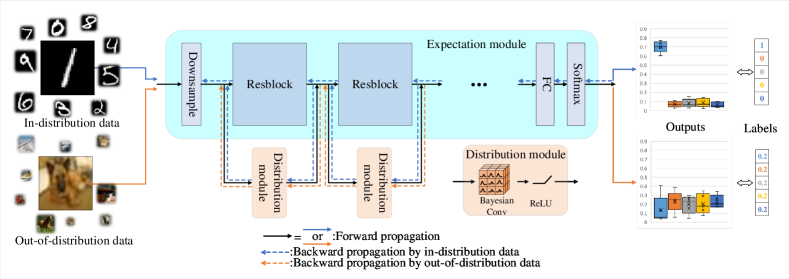
Figure 2: Components of ABNN. We take ResNet as the backbone and attach a distribution module to each Resblock. For out-of-distribution data, our network can catch its uncertainty and generate probabilistic results with large variances. For in-distribution data, our network can predict results with small variances.

We want to train our BNN on OOD data by maximizing $\mathbb{D}_{KL}[q(\omega|\mu,\sigma^{2})\\ ||p(\omega|\mathcal{D}_{\rm{OOD}})]$. However, this operation not only increases $\sigma^{2}$ but also changes $\mu$. If we train a traditional BNN by our methodology, the classification accuracy on ID data will drop, which is shown by our ablation experiment. To keep high performance on ID data, we try to separate the prediction ability and uncertainty estimation ability of a BNN, and design an attached structure. ABNN is composed of two kinds of modules: an expectation module and some distribution modules. For easy understanding, we take ResNet as the backbone model for illustration. A straightforward benefit of the attachment structure is that the backbone can be changed into any network while the uncertainty estimation ability is decided by the attachments alone. We show how ABNN performs with different backbones in Section IV-D. The structure is shown in Figure 2.

The expectation module is constructed by common network layers, responsible for the original task. We have no constraints for the expectation module on OOD data, but we believe that it can classify semi-OOD data well due to the generalization ability of DNNs.

The distribution modules are constructed by Bayesian layers [11], fitting some specific layers’ posteriors given both ID data and OOD data. On $\mathcal{D}_{\rm{ID}}$, they catch uncertainty by minimizing the KL-divergence between variational distributions and the true posterior distributions. On $\mathcal{D}_{\rm{OOD}}$, they catch uncertainty by maximizing the variance of some parameters. Researchers show that just a few Bayesian layers can already catch enough uncertainty [20], so we only simulate the distributions of some specific layers. As a result, ABNN only contains a few Bayesian modules that are “attached” to a common DNN, demanding only a bit more resources.

The objective function for training ABNN is:

$$\mathop{\min}\limits_{\omega_{1}}\mathbb{E}_{x\sim\mathcal{D}_{\rm{ID}}}[\mathbb{E}[L(x)]]$$ (42)

$$+ \mathop{\min}\limits_{\omega_{2}}\mathbb{D}_{KL}[q(\omega|\mu,\sigma^{2})||p(\omega|\mathcal{D}_{\rm{ID}})]$$ (43)

$$+ \mathop{\max}\limits_{\omega_{2}}\alpha\cdot\mathbb{D}_{KL}[q(\omega|\mu,\sigma^{2})||p(\omega|\mathcal{D}_{\rm{OOD}})],$$ (44)

where $L$ is the loss function that depends on the task, $\omega_{1}$ is the parameters of the expectation module, $\omega_{2}$ is the parameters of distribution modules and $\alpha$ is a hyperparameter that guarantees the performance of ABNN on $\mathcal{D}_{\rm{ID}}$. $\alpha$ does not have a significant effect on the performance of ABNN, and we chose $\alpha=0.95$ for experiments. Detailed discussions of $\alpha$ is shown in Section IV-E. We only use one kind of OOD data for training.

During each iteration, we train ABNN in three steps: (1) First, distribution modules are frozen and $\mathbb{E}_{x\sim\mathcal{D}_{\rm{ID}}}[\mathbb{E}[L(x)]]$ is minimized; (2) Then, the expectation module is frozen, and we minimize $\mathbb{D}_{KL}[q(\omega|\mu,\sigma^{2})||p(\omega|\mathcal{D}_{\rm{ID}})]$; (3) At last, we keep freezing the expectation module and maximize $\alpha\cdot\mathbb{D}_{KL}[q(\omega|\mu,\sigma^{2})||p(\omega|\mathcal{D}_{\rm{OOD}})]$.

Our training procedure is actually an EM algorithm [39, 40]: We divide the parameters of BNNs from $\omega=(\mu,\sigma^{2})$ into $(\omega_{1},\omega_{2})=((\mu_{1},\mu_{2}),(\sigma_{1}^{2},\sigma_{2}^{2}))$. We try to find the expectation $\mu_{1}$ of $\omega_{1}$ as the latent variables that guarantee predictive ability and find $(\mu_{2},\sigma_{2}^{2})$ as a balanced distribution between $p(\omega|\mathcal{D}_{\rm{ID}})$ and $p(\omega|\mathcal{D}_{\rm{OOD}})$. EM algorithms are sensitive to the initial value of latent variables, but ABNN can be well initialized by pre-training. Our training process is summarized in Algorithm 1.

Algorithm 1 Training of ABNN. $f_{\omega}(\cdot)$ is the whole network, $\omega=(\omega_{1},\omega_{2})$, $\omega_{1}$ represents parameters of expectation modules, $\omega_{2}=(\mu,\sigma^{2})$ represents parameters of distribution modules, $N$ is the number of forward propagation times, L is a loss function.

  Initialize $f_{\omega}(\cdot)$

  for training iterations do

     Sample minibatch data $X_{\rm{ID}}$ from $\mathcal{D}_{\rm{ID}}$

     for i=1; i$\leqslant$N; i++ do

        Sample $\epsilon^{i}$ from $\mathcal{N}(0,1)$

        $\omega_{2}^{i}=\mu+\sigma\epsilon^{i}$

        $\omega^{i}=(\omega_{1},\omega_{2}^{i})$

        Update $\omega_{1}$ by $\mathop{\min}L(f_{\omega^{i}}(X_{\rm{ID}}))$

     end for

     Update $\omega_{2}$ by $\mathop{\min}\sum_{i=1}^{N}log(q(\omega^{i}|\mu,\sigma^{2}))-log(p(\omega^{i}))-log(p(X_{\rm{ID}}|\omega^{i}))$

     Sample minibatch data $X_{\rm{OOD}}$ from $\mathcal{D}_{\rm{OOD}}$

     for i=1; i$\leqslant$N; i++ do

        Sample $\epsilon^{i}$ from $\mathcal{N}(0,1)$

        $\omega_{2}^{i}=\mu+\sigma\epsilon^{i}$

        $\omega^{i}=(\omega_{1},\omega_{2}^{i})$

     end for

     Update $\omega_{2}$ by $\mathop{\max}\alpha\sum_{i=1}^{N}log(q(\omega^{i}|\mu,\sigma^{2}))-log(p(\omega^{i}))-log(p(X_{\rm{OOD}}|\omega^{i}))$

  end for

Here we explain why our training procedure catches the appropriate amount of uncertainty. The ID training and OOD training are adversarial. We hope to increase the variance of some parameters to represent OOD uncertainty while maintaining performance on ID data, which means $q(\omega|\mu,\sigma^{2})$ should still fit $p(\omega|\mathcal{D}_{\rm{ID}})$ well. The third loss term is designed in the same formula as the second one and is regulated by a hyperparameter, so the changing rate of parameters during OOD training will not be greater than that during ID training. As a result, only parameters that have minimal impact on $\mathbb{D}_{KL}[q(\omega|\mu,\sigma^{2})||p(\omega|\mathcal{D}_{\rm{ID}})]$ (e.g. convs that fail to catch meaningful features from ID data) can be primarily optimized by OOD loss. During testing, the more OOD features an input includes, the more parameters with high variance (e.g. convs that only catch OOD features) will be activated, resulting in increased uncertainty. Furthermore, we show in Section III-C that the two latter loss terms can still be interpreted as a traditional BNN loss.

III-C Reinterpretation of Loss Terms

Although ABNN is trained on ID data and OOD data separately, we show that it is still under the Bayesian Learning framework. The second and third loss terms can be merged into one KL divergence.

From Theorem 8, we can get

$$\mathop{\arg\max}\limits_{\mu,\sigma^{2}}\mathbb{D}_{KL}[q(\omega|\mu,\sigma^{2})||p(\omega|\mathcal{D}_{\rm{OOD}})]$$ (45)

$$= \mathop{\arg\max}\limits_{\mu,\sigma^{2}}\mathbb{D}_{KL}[q(\omega|\mu,\sigma^{2})||p(\omega)]$$ (46)

$$-\int q(\omega|\mu,\sigma^{2})log(p(\mathcal{D}_{\rm{OOD}}|\omega))\,d\omega.$$ (47)

Similar,

$$\mathop{\arg\min}\limits_{\mu,\sigma^{2}}\mathbb{D}_{KL}[q(\omega|\mu,\sigma^{2})||p(\omega|\mathcal{D}_{\rm{ID}})]$$ (48)

$$= \mathop{\arg\min}\limits_{\mu,\sigma^{2}}\mathbb{D}_{KL}[q(\omega|\mu,\sigma^{2})||p(\omega)]$$ (49)

$$-\int q(\omega|\mu,\sigma^{2})log(p(\mathcal{D}_{\rm{ID}}|\omega))\,d\omega.$$ (50)

The first term works like a normalization and the second term is the initial loss function (e.g. cross entropy).

$$\mathop{\min}\limits_{\mu,\sigma^{2}}\mathbb{D}_{KL}[q(\omega|\mu,\sigma^{2})||p(\omega|\mathcal{D}_{\rm{ID}})]$$ (51)

$$+\mathop{\max}\limits_{\mu,\sigma^{2}}\alpha\cdot\mathbb{D}_{KL}[q(\omega|\mu,\sigma^{2})||p(\omega|\mathcal{D}_{\rm{OOD}})]$$ (52)

$$= \mathop{\min}\limits_{\mu,\sigma^{2}}\mathbb{D}_{KL}[q(\omega|\mu,\sigma^{2})||p(\omega|\mathcal{D}_{\rm{ID}})]$$ (53)

$$-\alpha\cdot\mathbb{D}_{KL}[q(\omega|\mu,\sigma^{2})||p(\omega|\mathcal{D}_{\rm{OOD}})]$$ (54)

$$= \mathop{\min}\limits_{\mu,\sigma^{2}}(1-\alpha)\cdot\mathbb{D}_{KL}[q(\omega|\mu,\sigma^{2})||p(\omega)]$$ (55)

$$-\int q(\omega|\mu,\sigma^{2})(log(p(\mathcal{D}_{\rm{ID}}|\omega))$$ (56)

$$-\alpha\cdot log(p(\mathcal{D}_{\rm{OOD}}|\omega)))\,d\omega$$ (57)

$$= \mathop{\min}\limits_{\mu,\sigma^{2}}\mathbb{D}_{KL}[q(\omega|\mu,\sigma^{2})||p(\omega)]$$ (58)

$$-\int q(\omega|\mu,\sigma^{2})log(\frac{p(\mathcal{D}_{\rm{ID}}|\omega)}{p(\mathcal{D}_{\rm{OOD}}|\omega)^{\alpha}})^{\frac{1}{1-\alpha}}\,d\omega.$$ (59)

The second term can be interpreted as a transformation of initial loss terms, and if we assume $p(D|\omega)=(\frac{p(\mathcal{D}_{\rm{ID}}|\omega)}{p(\mathcal{D}_{\rm{OOD}}|\omega)^{\alpha}})^{\frac{1}{1-\alpha}},\alpha\in(0,1)$,the objective functions can be reinterpreted as

$$\mathop{\min}\limits_{\mu,\sigma^{2}}\mathbb{D}_{KL}[q(\omega|\mu,\sigma^{2})||p(\omega|\mathcal{D}_{\rm{ID}})]$$ (60)

$$+\mathop{\max}\limits_{\mu,\sigma^{2}}\alpha\cdot\mathbb{D}_{KL}[q(\omega|\mu,\sigma^{2})||p(\omega|\mathcal{D}_{\rm{OOD}})]$$ (61)

$$= \mathop{\min}\limits_{\mu,\sigma^{2}}\mathbb{D}_{KL}[q(\omega|\mu,\sigma^{2})||p(\omega|D)].$$ (62)

IV Experiments

In this section, we evaluate the uncertainty estimation ability of ABNN through five groups of experiments. All experiments share the same setup, where the backbone is ResNet18 and the models are trained using Adam optimizer. The hyperparameters of all methods are set according to their default values and the $\alpha$ for ABNN is 0.95. The influence of $\alpha$ is shown in Section IV-E. Additionally, all models are trained by the same pseudo OOD data (constructed by adding Gaussian noise to ID data, without any additional information), which means all methods cannot see the real OOD data before test. The iteration times of SDE-Net are set to be the same as the residual block numbers of ABNN and other methods. For methods that need sampling, we sample 5 times at each training step.

IV-A Quantification Experiment

In Section III-B, we provide a brief explanation that ABNN can describe the continued growth of the uncertainty, and here we prove it with experiments. In real-world scenarios, a model can still work on semi-OOD data with a declined accuracy, while losing power on full-OOD data. Therefore, it is necessary to assess a model’s ability to differentiate between ID, semi-OOD and full-OOD data.

We show uncertainty by the max value of the prediction vectors after softmax layers, which is usually seen as the probability of the input belonging to its respective class. However, there is no such widely adopted metric for this triple classification. Inspired by ideas in unsupervised learning [41, 42], we propose a metric based on clustering. ID, semi-OOD and full-OOD can be seen as three clusters. If the predictions on the entire data space can be clustered into three groups correctly, the model is powerful at uncertainty estimation.

We set two experiments. In the first experiment, we assign MNIST as ID data, SVHN as semi-OOD data, and CIFAR10 as full-OOD data; in the second experiment, we build “Cat-Dog”, “Tiger-Wolf” datasets from CIFAR10 and CIFAR100 to serve as ID and semi-OOD data, and use other unrelated CIFAR images as full-OOD data. For a comprehensive evaluation, we utilized confusion matrices and density histograms to show the clustering results. To avoid taking the worst ID results and the best full-OOD results for unfair clustering, we remove predictions with extreme uncertainty from each dataset.

Our compared methods are: (1)BBP, traditional BNN; (2)VBOE, a BNN that combines frequentist training, and we choose the most related OOD training strategy (3) SDE-Net, a OOD detection specified method which shares similar structure and training process with ABNN; (4)OE, one of the most typical OOD training method; (5)WOODS, a variation of OE and get state of the art OOD detection performance.

All methods share the same backbone (besides SDE-Net, but we make a fair adaption) and same training procedure. All methods that need OOD training get OOD data by adding noises to ID data.

The quantitative results are listed in Table I and Table II. We report the average performance for 5 random initializations. As shown, all methods can treat ID data well. Since BBP only uses ID data for training, it can hardly recognize semi-OOD data and even full-OOD data. Besides BBP and WOODS, all the other methods can somehow recognize semi-OOD data and full-OOD data, but they still recognize many semi-OOD data either as ID data or full-OOD data. Among them, ABNN get the best overall results. WOODS achieve a perfect result in Table II, but its classification accuracy is only 64.7% on training set (92.5% for ABNN), which means WOODS may sacrifice prediction ability.

TABLE I: Cluster results on MNIST, SVHN and CIFAR10.

Model	BBP			VBOE			SDE-Net			OE			WOODS			ABNN
Confusion matrix	9000	0	0	9000	0	0	9000	0	0	9000	0	0	9000	0	0	9000	0	0
	9000	0	0	5929	3071	0	713	320	7967	9000	0	0	1183	7817	0	5894	3106	0
	3850	2689	2461	1881	2800	4319	9	19	8972	4104	2506	2390	338	7797	865	1253	1457	6290
Accuracy	42.4%			60.7%			67.7%			42.2%			65.5%			68.1%

TABLE II: Cluster results on CIFAR10 and CIFAR100.

Model	BBP			VBOE			SDE-Net			OE			WOODS			ABNN
Confusion matrix	100	0	0	100	0	0	100	0	0	100	0	0	100	0	0	100	0	0
	5	37	58	5	95	0	3	82	15	10	90	0	4	96	0	9	91	0
	0	84	16	0	44	56	0	46	54	0	38	62	0	0	100	0	32	68
Accuracy	51.0%			83.7%			68.7%			84.0%			98.7%			86.3%

The qualitative results are show in Figure 3 and Figure 4. We estimate uncertainty distributions by frequency in the top row and list all predictions by order to show the increasing trend of uncertainty in the bottom row. The Ideal visualization is draw manually, following the rule that uncertainty should increase gradually but be separable on semi-OOD and full-OOD datasets. As shown in Figure 3, besides ABNN, SDE-Net and WOODS, all methods give too low uncertainty estimation for semi-OOD data, and SDE-Net gives too high uncertainty estimate for semi-OOD data. Although WOODS can separate ID, semi-OOD and full-OOD data well, it still gives too many low estimates for full-OOD data and gives too high estimates for ID data. It’s surprising that OE methods still gives low uncertainty estimation for semi-OOD data, and we find this is because we use pseudo OOD data(ID data added noises) for OOD training. If we use true OOD data or pseudo data with greater noises, their visualizations will be like SDE-Net’s. As shown in Figure 4, BBP and SDE-Net mix up semi-OOD and full-OOD data. VBOE and OE can somehow distinguish semi-OOD and full-OOD data, but there are still overlapped uncertainty. WOODS can well distinguish different data, but it gives too high estimation for ID uncertainty. Although there are some mixed data, ABNN treat different uncertainties better than other models do.

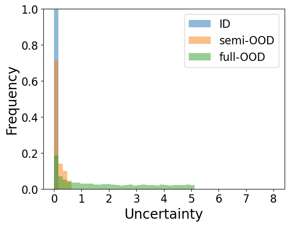
(a) BBP

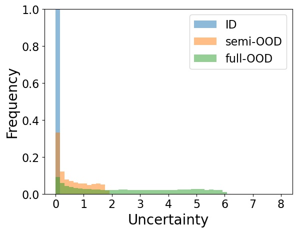
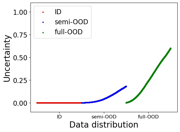
(b) VBOE

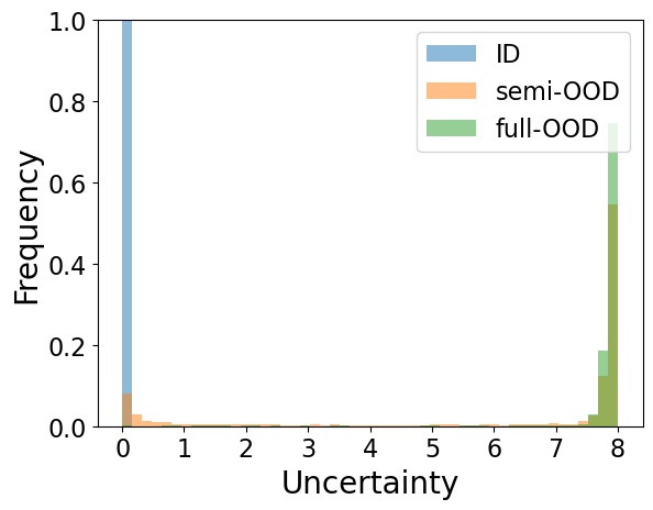
(c) SDE-Net

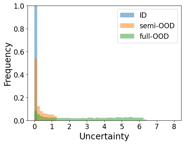
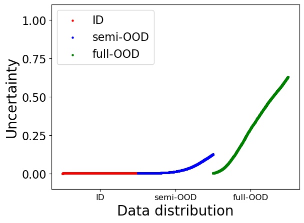
(d) OE

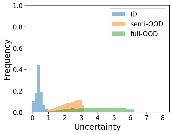
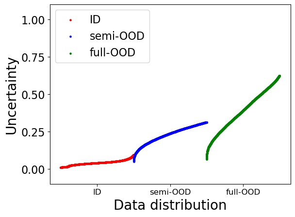
(e) WOODS

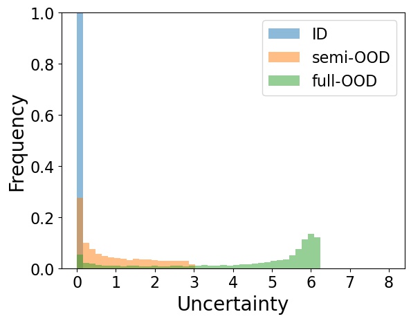
(f) ABNN

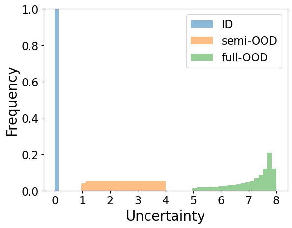
(g) Ideal

Figure 3: Uncertainty distributions on MNIST, SVHN and CIFAR10. The first row is uncertainty distributions; the second row is ordered uncertainty on different datasets. Distributions that are more separated indicate better performances.

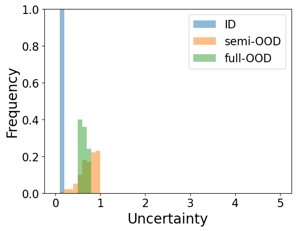
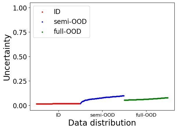
(a) BBP

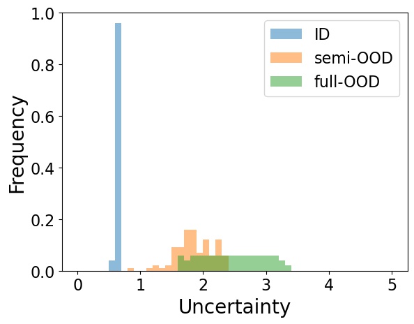
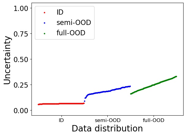
(b) VBOE

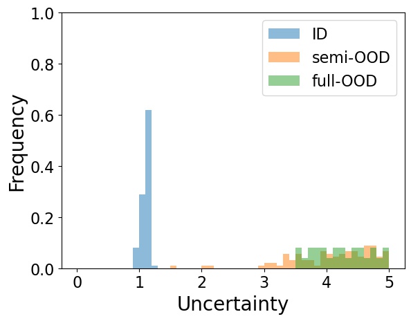
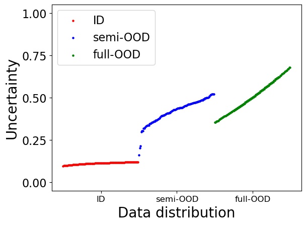
(c) SDE-Net

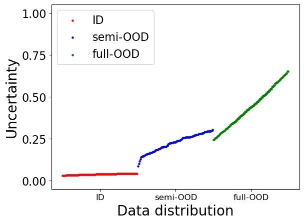
(d) OE

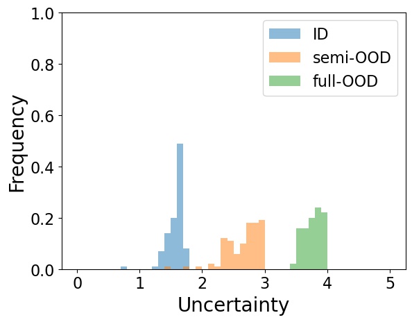
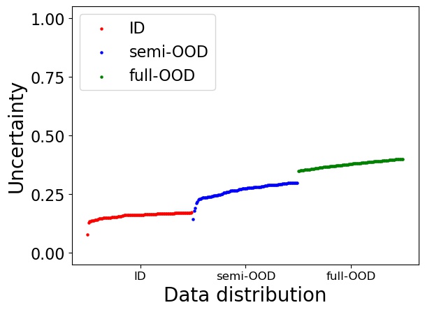
(e) WOODS

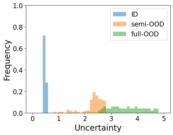
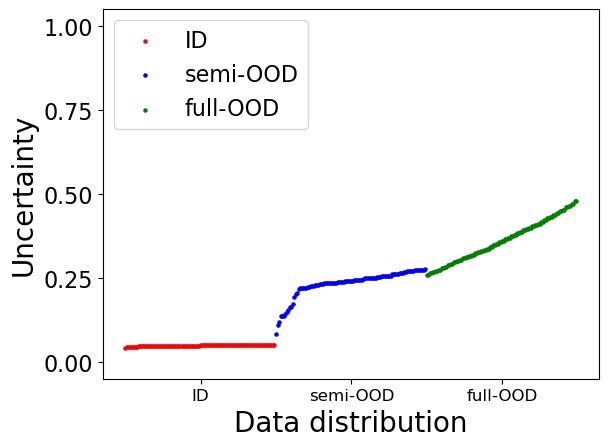
(f) ABNN

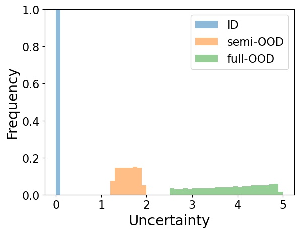
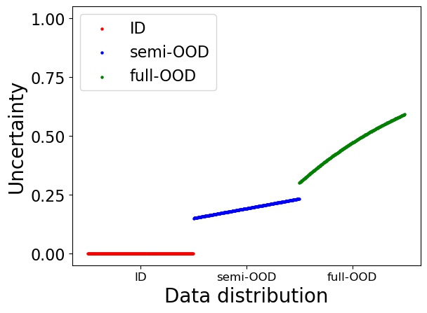
(g) Ideal

Figure 4: Uncertainty distributions on CIFAR10 and CIFAR100. The first row is uncertainty distributions; the second row is ordered uncertainty on different datasets. Distributions that are more separated indicate better performances.

IV-B Ablation Experiment

TABLE III: Effect of different strategies. We train ABNN on MNIST and take SVHN as OOD data. “OOD” means whether OOD data are used; “attachment” means whether the structure is an attachment version; “constant” means whether the labels are mean values or random variables; “maximize” means whether we maximize KL-divergence on $\mathcal{D}_{\rm{OOD}}$; “pseudo” means whether the OOD data is pseudo data or CIFAR10 during training.

Index	OOD	Attachment	Constant	Maximize	Pseudo	Classification accuracy	TNR at TPR 95%	AUROC	Detection accuracy	AUPR in	AUPR out
(a)	$\surd$	$\surd$	$\surd$	$\surd$	$\surd$	99.5$\pm$0.0	98.3$\pm$1.2	99.4$\pm$0.4	97.2$\pm$0.9	98.7$\pm$0.7	99.7$\pm$0.2
(b)	$\times$	$\surd$	$-$	$-$	$-$	99.4$\pm$0.0	91.7$\pm$2.3	97.6$\pm$0.6	94.0$\pm$1.1	94.8$\pm$2.6	98.8$\pm$0.1
(c)	$\surd$	$\times$	$\surd$	$\surd$	$\surd$	99.3$\pm$0.0	91.6$\pm$1.0	97.0$\pm$0.5	93.5$\pm$0.5	92.4$\pm$1.2	99.0$\pm$0.1
(d)	$\surd$	$\surd$	$\times$	$-$	$\surd$	99.5$\pm$0.1	55.9$\pm$20.4	94.2$\pm$2.2	92.3$\pm$2.5	91.6$\pm$2.5	96.7$\pm$1.3
(e)	$\surd$	$\surd$	$\surd$	$\times$	$\surd$	99.5$\pm$0.0	96.1$\pm$1.1	98.9$\pm$0.2	95.8$\pm$0.6	97.2$\pm$0.7	99.6$\pm$0.1
(f)	$\surd$	$\surd$	$\surd$	$\surd$	$\times$	99.5$\pm$0.0	100.0$\pm$0.0	98.7$\pm$0.6	99.2$\pm$0.3	99.1$\pm$0.4	97.6$\pm$1.0

We also conduct ablation studies to examine the contributions of different aspects of our method and identify any unnecessary strategies. We divide our method into five strategies: (1) whether OOD data are used; (2) whether the structure is an attachment version; (3) whether the labels are random versions or constant versions; (4)if labels are constant versions, whether we maximize KL-divergence or minimize KL-divergence on $\mathcal{D}_{\rm{OOD}}$; (5) whether the OOD data is from true dataset or pseudo ones.

Following previous work [43], we use (1) true negative rate (TNR) at 95% true positive rate (TPR); (2) area under the receiver operating characteristic curve (AUROC); (3) area under the precision-recall curve (AUPR); and (4) detection accuracy to evaluate performance. Larger values indicate better detection performance. We take MNIST as ID data and SVHN as OOD data. We report the average performance and standard deviation for 5 random initializations. The results are shown in Table III.

According to row (a) and row (b), adding OOD data during training time does help ABNN to catch more uncertainty. Row (a) and row(c) suggest that without an attachment structure, ABNN will not only harm the classification accuracy but also have worse uncertainty estimation ability. Row (d) shows that if we use random variables as training labels for OOD data, the training process will be instable, and we will get a model with poor uncertainty estimation ability. Row (a) and row (e) verify our assumption that maximizing the KL-divergence on OOD data can converge and make a more powerful model. According to row (f), we find that using true datasets as OOD data during training can bring some improvements, but it also brings some drops under several metrics. Compared with results in Table IV, we find that ABNN outperforms many other models overall. In real-world scenes, one can choose how to build $\mathcal{D}_{\rm{OOD}}$ by convenience. In conclusion, all strategies are necessary.

IV-C Applications

In this section, we show how ABNN performs in traditional tasks. We compare ABNN with the following uncertainty estimate or OOD detection methods: (1) Threshold [43], (2) DeepEnsemble [44], (3) OE [24], a classical OOD training method, (4) WOODS [23], a variant of OE that achieves state-of-the-art OOD detection performance, (5)SDE-Net [25], which shares similar structure and training process with ABNN but is designed especially for OOD detection, (6) BBP [11], a classical variational inference BNN, (7) p-SGLD [13], a Markov chain Monte Carlo BNN, and (8) VBOE [22], a BNN that includes OOD training like OE. We keep using Hendrycks’ metrics [43].

IV-C1 OOD Detection

TABLE IV: Classification and out-of-distribution detection results. All values are in percentage, and larger values indicates better performance. We mark non-Bayesian models by $\star$ and Bayesian models by $\diamond$. We use bold font to highlight the best results in both groups. ABNN can achieve comparable performances to OOD detection specialized models.

ID	OOD	Model	Parameters	Classification accuracy	TNR at TPR 95%	AUROC	Detection accuracy	AUPR in	AUPR out
MNIST	SEMEION	Threshold$\star$	0.58M	99.5$\pm$0.0	94.0$\pm$1.4	98.3$\pm$0.3	94.8$\pm$0.7	99.7$\pm$0.1	89.4$\pm$1.1
		DeepEnsemble$\star$	0.58M$\times$5	99.6$\pm$NA	96.0$\pm$NA	98.8$\pm$NA	95.8$\pm$NA	99.8$\pm$NA	91.3$\pm$NA
		OE$\star$	0.58M	99.5$\pm$0.1	96.3$\pm$0.5	98.7$\pm$0.1	95.9$\pm$0.2	99.8$\pm$0.0	90.8$\pm$0.5
		WOODS$\star$	0.58M	99.3$\pm$0.0	86.4$\pm$0.4	97.4$\pm$0.1	95.2$\pm$0.2	99.6$\pm$0.0	87.7$\pm$0.7
		SDE-Net$\star$	0.28M	99.4$\pm$0.1	99.6$\pm$0.2	99.9$\pm$0.1	98.6$\pm$0.5	100.0$\pm$0.0	99.5$\pm$0.3
		BBP$\diamond$	0.58M$\times$2	99.2$\pm$0.3	75.0$\pm$3.4	94.8$\pm$1.2	90.4$\pm$2.2	99.2$\pm$0.3	76.0$\pm$4.2
		p-SGLD$\diamond$	0.58M	99.3$\pm$0.2	85.3$\pm$2.3	89.1$\pm$1.6	90.5$\pm$1.3	93.6$\pm$1.0	82.8$\pm$2.2
		VBOE$\diamond$	0.58M$\times$2	99.5$\pm$0.2	96.0$\pm$0.2	99.0$\pm$0.0	95.4$\pm$0.2	99.9$\pm$0.0	93.6$\pm$0.3
		ABNN$\diamond$	0.58M+0.30M	99.5$\pm$0.0	97.9$\pm$0.7	99.2$\pm$0.1	96.9$\pm$0.5	99.0$\pm$0.0	95.0$\pm$1.2
MNIST	SVHN	Threshold$\star$	0.58M	99.5$\pm$0.0	90.1$\pm$2.3	96.8$\pm$0.9	92.9$\pm$1.1	90.0$\pm$3.3	98.7$\pm$0.3
		DeepEnsemble$\star$	0.58M$\times$5	99.6$\pm$NA	92.7$\pm$NA	98.0$\pm$NA	94.1$\pm$NA	94.5$\pm$NA	99.1$\pm$NA
		OE$\star$	0.58M	99.5$\pm$0.1	92.1$\pm$1.2	97.5$\pm$0.4	93.7$\pm$0.6	93.1$\pm$1.3	99.0$\pm$0.2
		WOODS$\star$	0.58M	99.3$\pm$0.0	94.2z$\pm$1.6	98.0$\pm$0.2	96.0$\pm$0.2	97.6$\pm$0.2	98.6$\pm$0.2
		SDE-Net$\star$	0.28M	99.4$\pm$0.1	97.8$\pm$1.1	99.5$\pm$0.2	97.0$\pm$0.2	98.6$\pm$0.6	99.8$\pm$0.1
		BBP$\diamond$	0.58M$\times$2	99.2$\pm$0.3	80.5$\pm$3.2	96.0$\pm$1.1	91.9$\pm$0.9	92.6$\pm$2.4	98.3$\pm$0.4
		p-SGLD$\diamond$	0.58M	99.3$\pm$0.2	94.5$\pm$2.1	95.7$\pm$1.3	95.0$\pm$1.2	75.6$\pm$5.2	98.7$\pm$0.2
		VBOE$\diamond$	0.58M$\times$2	99.5$\pm$0.0	98.1$\pm$0.2	99.5$\pm$0.1	97.6$\pm$0.2	98.0$\pm$0.1	99.8$\pm$0.0
		ABNN$\diamond$	0.58M+0.30M	99.5$\pm$0.0	98.3$\pm$1.2	99.4$\pm$0.4	99.5$\pm$0.2	98.7$\pm$0.7	99.7$\pm$0.2
SVHN	CIFAR10	Threshold$\star$	0.58M	95.2$\pm$0.1	66.1$\pm$1.9	94.4$\pm$0.4	89.8$\pm$0.5	96.7$\pm$0.2	84.6$\pm$0.8
		DeepEnsemble$\star$	0.58M$\times$5	95.4$\pm$NA	66.5$\pm$NA	94.6$\pm$NA	90.1$\pm$NA	97.8$\pm$NA	84.8$\pm$NA
		OE$\star$	0.58M	95.2$\pm$0.0	67.8$\pm$2.8	94.9$\pm$0.5	90.2$\pm$0.5	98.0$\pm$0.2	85.8$\pm$1.3
		WOODS$\star$	0.58M	94.3$\pm$0.1	57.9$\pm$1.5	94.1$\pm$0.2	88.6$\pm$0.2	97.8$\pm$0.1	82.7$\pm$0.4
		SDE-Net$\star$	0.32M	94.2$\pm$0.2	87.5$\pm$2.8	97.8$\pm$0.4	92.7$\pm$0.7	99.2$\pm$0.2	93.7$\pm$0.9
		BBP$\diamond$	0.58M$\times$2	93.3$\pm$0.6	42.2$\pm$1.2	90.4$\pm$0.3	83.9$\pm$0.4	96.4$\pm$0.2	73.9$\pm$0.5
		p-SGLD$\diamond$	0.58M	94.1$\pm$0.5	63.5$\pm$0.9	94.3$\pm$0.4	87.8$\pm$1.2	97.9$\pm$0.2	83.9$\pm$0.7
		VBOE$\diamond$	0.58M$\times$2	95.1$\pm$0.2	61.8$\pm$1.1	93.7$\pm$0.3	88.7$\pm$0.4	97.3$\pm$0.2	83.0$\pm$0.6
		ABNN$\diamond$	0.58M+0.30M	95.3$\pm$0.3	72.8$\pm$2.4	96.0$\pm$0.4	90.7$\pm$0.5	98.5$\pm$0.1	88.5$\pm$1.1
SVHN	CIFAR100	Threshold$\star$	0.58M	95.2$\pm$0.1	64.6$\pm$1.9	93.8$\pm$0.4	88.3$\pm$0.4	97.0$\pm$0.2	83.7$\pm$0.8
		DeepEnsemble$\star$	0.58M$\times$5	95.4$\pm$NA	64.4$\pm$NA	93.9$\pm$NA	89.4$\pm$NA	97.4$\pm$NA	84.8$\pm$NA
		OE$\star$	0.58M	95.2$\pm$0.0	65.3$\pm$2.7	94.4$\pm$0.5	89.6$\pm$0.4	97.7$\pm$0.3	84.8$\pm$1.2
		WOODS$\star$	0.58M	94.3$\pm$0.1	58.8$\pm$1.5	93.6$\pm$0.2	88.0$\pm$0.1	97.6$\pm$0.1	81.9$\pm$0.5
		SDE-Net$\star$	0.32M	94.2$\pm$0.2	83.4$\pm$3.6	97.0$\pm$0.4	91.6$\pm$0.7	98.8$\pm$0.1	92.3$\pm$1.1
		BBP$\diamond$	0.58M$\times$2	93.3$\pm$0.6	42.4$\pm$0.3	90.6$\pm$0.2	84.3$\pm$0.3	96.5$\pm$0.1	75.2$\pm$0.9
		p-SGLD$\diamond$	0.58M	94.1$\pm$0.5	62.0$\pm$0.5	91.3$\pm$1.2	86.0$\pm$0.2	93.1$\pm$0.8	81.9$\pm$1.3
		VBOE$\diamond$	0.58M$\times$2	95.1$\pm$0.2	60.4$\pm$1.1	93.3$\pm$0.3	88.2$\pm$0.4	97.1$\pm$0.2	82.3$\pm$0.6
		ABNN$\diamond$	0.58M+0.30M	95.3$\pm$0.3	70.1$\pm$0.6	95.2$\pm$0.3	91.1$\pm$0.3	99.0$\pm$0.2	89.2$\pm$0.8

OOD detection is a significant application of uncertainty estimation [45, 46]. In real-world scenarios, when OOD samples are presented to a model, e.g. give a dog image to an MNIST classification model, we hope the model says ’I don’t know’ instead of making a prediction blindly. A neural network can distinguish ID and OOD data by uncertainty estimation: ID data usually bring lower uncertainty while OOD data tend to present higher uncertainty.

We set 4 groups of experiments by choosing different datasets to be ID and OOD data: (1) MNIST vs SEMEION, (2) MNIST vs SVHN, (3) SVHN vs CIFAR10, (4) SVHN vs CIFAR100. As shown in Table IV, ABNN achieves the best results compared with traditional BNNs. Although ABNN is not designed specifically for OOD detection, it is still comparable with SDE-Net and even outperforms it under some metrics. Besides SDE-Net, ABNN is far better than traditional BNNs and other OOD detection models.

Classification accuracy is also an important metric. As shown in Table IV, traditional BNNs may harm the predictive power, but ABNN can still make accurate classifications. We also count the amount of parameters in Table IV. Variational inference BNNs double the amount of parameters. P-SGLD has to store copies of the parameters for evaluation, which is prohibitively costly. Although ABNN is a Bayesian method, it just needs a few more parameters due to the attachment structure.

IV-C2 Misclassification Detection

TABLE V: Misclassification detection performance. We report the average performance and standard deviation for 5 random initializations.

Data	Model	TNR at TPR 95%	AUROC	Detection accuracy	AUPR succ	AUPR err
MNIST	Threshold	85.4$\pm$2.8	94.3$\pm$0.9	92.1$\pm$1.5	99.8$\pm$0.1	31.9$\pm$8.3
	DeepEnsemble	89.6$\pm$NA	97.5$\pm$NA	93.2$\pm$NA	100.0$\pm$NA	41.4$\pm$NA
	OE	88.4$\pm$2.1	96.2$\pm$0.5	92.8$\pm$0.9	100.0$\pm$0.0	32.9$\pm$7.9
	WOODS	85.1$\pm$0.8	97.0$\pm$0.1	92.3$\pm$0.5	99.9$\pm$0.0	43.2$\pm$3.1
	SDE-Net	88.5$\pm$1.3	96.8$\pm$0.9	92.9$\pm$0.8	100.0$\pm$0.0	36.6$\pm$4.6
	BBP	88.7$\pm$0.9	96.5$\pm$2.1	93.1$\pm$0.5	100.0$\pm$0.0	35.4$\pm$3.2
	p-SGLD	93.2$\pm$2.5	96.4$\pm$1.7	98.4$\pm$0.2	100.0$\pm$0.0	42.0$\pm$2.4
	VBOE	85.1$\pm$4.3	94.6$\pm$0.9	91.5$\pm$1.9	100.0$\pm$0.0	31.4$\pm$1.8
	ABNN	92.4$\pm$2.1	98.4$\pm$0.5	95.3$\pm$0.7	99.7$\pm$0.1	36.2$\pm$0.5
	ABNN(CIFAR10)	93.9$\pm$2.6	98.7$\pm$0.3	97.5$\pm$1.2	100.0$\pm$0.0	37.8$\pm$4.6
SVHN	Threshold	66.4$\pm$1.7	90.1$\pm$0.3	85.9$\pm$0.4	99.3$\pm$0.0	42.8$\pm$0.6
	DeepEnsemble	67.2$\pm$NA	91.0$\pm$NA	86.6$\pm$NA	99.4$\pm$NA	46.5$\pm$NA
	OE	64.5$\pm$1.3	91.4$\pm$0.6	86.3$\pm$0.6	99.4$\pm$0.1	45.3$\pm$1.8
	WOODS	63.9$\pm$1.2	92.6$\pm$0.1	86.9$\pm$0.3	99.4$\pm$0.0	48.6$\pm$1.9
	SDE-Net	65.6$\pm$1.9	92.3$\pm$0.5	86.8$\pm$0.4	99.4$\pm$0.0	53.9$\pm$2.5
	BBP	58.7$\pm$2.1	91.8$\pm$0.2	85.6$\pm$0.7	99.1$\pm$0.1	50.7$\pm$0.9
	p-SGLD	64.2$\pm$1.3	93.0$\pm$0.4	87.1$\pm$0.4	99.4$\pm$0.1	48.6$\pm$1.8
	VBOE	63.4$\pm$1.0	90.5$\pm$0.1	84.8$\pm$0.3	99.3$\pm$0.0	44.6$\pm$1.5
	ABNN	67.1$\pm$2.8	92.9$\pm$0.3	86.7$\pm$0.3	99.4$\pm$0.1	50.2$\pm$1.8
	ABNN(CIFAR10)	67.3$\pm$1.8	93.2$\pm$0.2	87.9$\pm$0.3	99.5$\pm$0.1	52.4$\pm$1.8

Misclassification detection is another important application of uncertainty estimation [47, 48]. Similar to OOD detection, outputs with low uncertainty are more likely to be classified correctly and those with high uncertainty are probably misclassified. As the use of real OOD data during training does not impact fairness, we also evaluate the performance of ABNN trained with CIFAR10 as OOD data.

As shown in Table V, if not trained with real OOD data, p-SGLD achieves the best performance overall, and ABNN is comparable to it. However, if we fully explore ABNN’s power, ABNN gets the best results.

IV-D ABNN with different backbone

We choose to use ResNet as our backbone for two reasons: (1) its ease of understanding, and (2) the fact that some of our competitor models rely on ResNet as their backbone. However, our theories and optimization procedures are not dependent on the structure of the networks, and thus ABNN can be easily generalized to other BNN structures. The backbone network is focused on classification, while the estimation of uncertainty is largely determined by the configuration of the distribution modules, rather than the architecture of the backbone. Another advantage of ABNN is that the expectation module can be frozen, which means we only need to train the small-sized distribution modules. We show by experiments how ABNN performs with different backbones:

TABLE VI: Misclassification detection performance on different backbones. We report the average performance and standard deviation for 5 random initializations.

Backbone	Classification accuracy	TNR at TPR 95%	AUROC	Detection accuracy	AUPR succ	AUPR err
ResNet18	99.5$\pm$0.0	98.3$\pm$1.2	99.4$\pm$0.4	99.5$\pm$0.2	98.7$\pm$0.7	99.7$\pm$0.2
MobileNet V3	99.5$\pm$0.1	98.3$\pm$0.9	99.6$\pm$0.2	99.2$\pm$0.3	98.7$\pm$1.1	99.8$\pm$0.1
EfficientNet V2	99.6$\pm$0.2	98.0$\pm$1.1	99.5$\pm$0.3	99.2$\pm$0.2	97.9$\pm$0.3	99.4$\pm$0.6
SqueezeNet	99.5$\pm$0.1	98.2$\pm$1.3	99.6$\pm$0.3	99.5$\pm$0.5	98.2$\pm$0.4	99.6$\pm$0.1

IV-E Function of $\alpha$

Although $\alpha$ seems to balance the uncertainty obtained from ID and OOD data, its true function is to determine the relationship between uncertainty and variance. As shown in Theorem 8, the OOD training attempts to enlarge the variance to $\infty$, but the ID training limits the variance. As a result, there is an adversarial training that finally defines how large the variance can be. The largest variance is the representation of the greatest uncertainty. Therefore, $\alpha$ implicitly defines how much uncertainty is represented by one level of variance. We can show by experiments that the choice of $\alpha$ would not hurt the uncertainty estimation ability of ABNN:

TABLE VII: Misclassification detection performance with different $\alpha$. We report the average performance and standard deviation for 5 random initializations.

$\alpha$	Classification accuracy	TNR at TPR 95%	AUROC	Detection accuracy	AUPR succ	AUPR err
0.5	99.5$\pm$0.0	98.8$\pm$1.8	99.2$\pm$0.4	98.2$\pm$0.9	97.7$\pm$1.0	99.4$\pm$0.2
0.7	99.5$\pm$0.0	98.0$\pm$0.9	98.8$\pm$0.3	99.2$\pm$0.5	97.6$\pm$0.5	99.4$\pm$0.3
0.9	99.5$\pm$0.0	98.4$\pm$1.1	99.4$\pm$0.3	99.3$\pm$0.8	98.7$\pm$0.7	99.7$\pm$0.2
0.95	99.5$\pm$0.0	98.3$\pm$1.2	99.4$\pm$0.4	99.5$\pm$0.2	98.7$\pm$0.7	99.7$\pm$0.2
1	99.5$\pm$0.0	98.4$\pm$0.8	99.5$\pm$0.3	99.4$\pm$0.7	98.8$\pm$0.5	99.8$\pm$0.2

V Discussions

Our segmentations and definitions are based on the assumption that the classification task is consistent with the estimation of the target distribution of each class. We did not show an approach to quantify the validity of the uncertainty estimation for ABNN. This problem may be solved by examining the second loss term, $\mathbb{D}_{KL}[q(\omega|\mu,\sigma^{2})||p(\omega|\mathcal{D}_{\rm{ID}})]$. Without the third loss term, the ID KL-divergence should be optimized to its minimum, which implies that the distribution modules are the best estimations of the ID posteriors. However, the third loss term will increase some variances, so the increase in the ID KL-divergence indicates how much OOD uncertainty is captured and whether ABNN can still maintain its performance on ID data.

VI Conclusion

We propose a variational inference Bayesian Neural Network with an attachment structure to catch more uncertainty from OOD data. We provide mathematical descriptions for OOD data and design the attachment structure for proper integration of uncertainty. The convergence of ABNN is theoretically analyzed. The experiments show ABNN’s superiority over traditional BNNs. In the future, we will pay attention to developing a more effective method to catch the uncertainty from OOD data. Overall, our proposed method can be considered as a framework, where the attachment structure can be extended to other general BNNs.

References

- [1] Yinglong Li. Research and application of deep learning in image recognition. In 2022 IEEE 2nd International Conference on Power, Electronics and Computer Applications (ICPECA), pages 994–999. IEEE, 2022.
- [2] Spilios Evmorfos, Konstantinos I Diamantaras, and Athina P Petropulu. Reinforcement learning for motion policies in mobile relaying networks. IEEE Transactions on Signal Processing, 70:850–861, 2022.
- [3] Ivano Lauriola, Alberto Lavelli, and Fabio Aiolli. An introduction to deep learning in natural language processing: Models, techniques, and tools. Neurocomputing, 470:443–456, 2022.
- [4] Moloud Abdar, Farhad Pourpanah, Sadiq Hussain, Dana Rezazadegan, Li Liu, Mohammad Ghavamzadeh, Paul Fieguth, Xiaochun Cao, Abbas Khosravi, U Rajendra Acharya, et al. A review of uncertainty quantification in deep learning: Techniques, applications and challenges. Information Fusion, 2021.
- [5] Saloua Chlaily, Debanshu Ratha, Pigi Lozou, and Andrea Marinoni. On measures of uncertainty in classification. IEEE Transactions on Signal Processing, pages 1–15, 2023.
- [6] Shixiong Wang and Zhi-Sheng Ye. Distributionally robust state estimation for linear systems subject to uncertainty and outlier. IEEE Transactions on Signal Processing, 70:452–467, 2022.
- [7] Yi Han and Thomas C. M. Lee. Uncertainty quantification for sparse estimation of spectral lines. IEEE Transactions on Signal Processing, 70:6243–6256, 2022.
- [8] Matthias Hein, Maksym Andriushchenko, and Julian Bitterwolf. Why relu networks yield high-confidence predictions far away from the training data and how to mitigate the problem. In Proceedings of the IEEE/CVF Conference on Computer Vision and Pattern Recognition, pages 41–50, 2019.
- [9] Hongxin Wei, Renchunzi Xie, Hao Cheng, Lei Feng, Bo An, and Yixuan Li. Mitigating neural network overconfidence with logit normalization. In International Conference on Machine Learning, pages 23631–23644. PMLR, 2022.
- [10] Anh Nguyen, Jason Yosinski, and Jeff Clune. Deep neural networks are easily fooled: High confidence predictions for unrecognizable images. In Proceedings of the IEEE conference on computer vision and pattern recognition, pages 427–436, 2015.
- [11] Charles Blundell, Julien Cornebise, Koray Kavukcuoglu, and Daan Wierstra. Weight uncertainty in neural network. In International Conference on Machine Learning, pages 1613–1622. PMLR, 2015.
- [12] Rahif Kassab and Osvaldo Simeone. Federated generalized bayesian learning via distributed stein variational gradient descent. IEEE Transactions on Signal Processing, 70:2180–2192, 2022.
- [13] Chunyuan Li, Changyou Chen, David Carlson, and Lawrence Carin. Preconditioned stochastic gradient langevin dynamics for deep neural networks. In Thirtieth AAAI Conference on Artificial Intelligence, 2016.
- [14] Ruqi Zhang, Andrew Gordon Wilson, and Christopher De Sa. Low-precision stochastic gradient langevin dynamics. In International Conference on Machine Learning, pages 26624–26644. PMLR, 2022.
- [15] Erik Daxberger, Agustinus Kristiadi, Alexander Immer, Runa Eschenhagen, Matthias Bauer, and Philipp Hennig. Laplace redux - effortless bayesian deep learning. In M. Ranzato, A. Beygelzimer, Y. Dauphin, P.S. Liang, and J. Wortman Vaughan, editors, Advances in Neural Information Processing Systems, volume 34, pages 20089–20103. Curran Associates, Inc., 2021.
- [16] Lisa Gaedke-Merzhäuser, Janet van Niekerk, Olaf Schenk, and Håvard Rue. Parallelized integrated nested laplace approximations for fast bayesian inference. Statistics and Computing, 33(1):25, 2023.
- [17] Achille Nazaret and David Blei. Variational inference for infinitely deep neural networks. In International Conference on Machine Learning, pages 16447–16461. PMLR, 2022.
- [18] Alex Graves. Practical variational inference for neural networks. Advances in neural information processing systems, 24, 2011.
- [19] Kumar Shridhar, Felix Laumann, and Marcus Liwicki. A comprehensive guide to bayesian convolutional neural network with variational inference. arXiv preprint arXiv:1901.02731, 2019.
- [20] Agustinus Kristiadi, Matthias Hein, and Philipp Hennig. Being bayesian, even just a bit, fixes overconfidence in relu networks. In International Conference on Machine Learning, pages 5436–5446. PMLR, 2020.
- [21] Yoshua Bengio, Frédéric Bastien, Arnaud Bergeron, Nicolas Boulanger-Lewandowski, Thomas Breuel, Youssouf Chherawala, Moustapha Cisse, Myriam Côté, Dumitru Erhan, Jeremy Eustache, et al. Deep learners benefit more from out-of-distribution examples. In Proceedings of the Fourteenth International Conference on Artificial Intelligence and Statistics, pages 164–172. JMLR Workshop and Conference Proceedings, 2011.
- [22] Agustinus Kristiadi, Matthias Hein, and Philipp Hennig. Being a bit frequentist improves bayesian neural networks. In International Conference on Artificial Intelligence and Statistics, pages 529–545. PMLR, 2022.
- [23] Julian Katz-Samuels, Julia B Nakhleh, Robert Nowak, and Yixuan Li. Training OOD detectors in their natural habitats. In Kamalika Chaudhuri, Stefanie Jegelka, Le Song, Csaba Szepesvari, Gang Niu, and Sivan Sabato, editors, Proceedings of the 39th International Conference on Machine Learning, volume 162 of Proceedings of Machine Learning Research, pages 10848–10865. PMLR, 17–23 Jul 2022.
- [24] Dan Hendrycks, Mantas Mazeika, and Thomas Dietterich. Deep anomaly detection with outlier exposure. arXiv preprint arXiv:1812.04606, 2018.
- [25] Lingkai Kong, Jimeng Sun, and Chao Zhang. Sde-net: Equipping deep neural networks with uncertainty estimates. arXiv preprint arXiv:2008.10546, 2020.
- [26] Chen Qiu, Aodong Li, Marius Kloft, Maja Rudolph, and Stephan Mandt. Latent outlier exposure for anomaly detection with contaminated data. In International Conference on Machine Learning, pages 18153–18167. PMLR, 2022.
- [27] Yifei Ming, Ying Fan, and Yixuan Li. Poem: Out-of-distribution detection with posterior sampling. In International Conference on Machine Learning, pages 15650–15665. PMLR, 2022.
- [28] Zehao Xiao, Jiayi Shen, Xiantong Zhen, Ling Shao, and Cees GM Snoek. A bit more bayesian: Domain-invariant learning with uncertainty. arXiv preprint arXiv:2105.04030, 2021.
- [29] Yann LeCun, Léon Bottou, Yoshua Bengio, and Patrick Haffner. Gradient-based learning applied to document recognition. Proceedings of the IEEE, 86(11):2278–2324, 1998.
- [30] Shiyu Liang, Yixuan Li, and Rayadurgam Srikant. Enhancing the reliability of out-of-distribution image detection in neural networks. arXiv preprint arXiv:1706.02690, 2017.
- [31] Yuval Netzer, Tao Wang, Adam Coates, Alessandro Bissacco, Bo Wu, and Andrew Y Ng. Reading digits in natural images with unsupervised feature learning. 2011.
- [32] Weitao Wan, Yuanyi Zhong, Tianpeng Li, and Jiansheng Chen. Rethinking feature distribution for loss functions in image classification. In Proceedings of the IEEE conference on computer vision and pattern recognition, pages 9117–9126, 2018.
- [33] Jiangtao Xie, Fei Long, Jiaming Lv, Qilong Wang, and Peihua Li. Joint distribution matters: Deep brownian distance covariance for few-shot classification. In Proceedings of the IEEE/CVF Conference on Computer Vision and Pattern Recognition (CVPR), pages 7972–7981, June 2022.
- [34] Jing Wang and Xin Geng. Classification with label distribution learning. In IJCAI, pages 3712–3718, 2019.
- [35] Bin-Bin Gao, Chao Xing, Chen-Wei Xie, Jianxin Wu, and Xin Geng. Deep label distribution learning with label ambiguity. IEEE Transactions on Image Processing, 26(6):2825–2838, 2017.
- [36] Alex Krizhevsky, Geoffrey Hinton, et al. Learning multiple layers of features from tiny images. 2009.
- [37] Yen-Chang Hsu, Yilin Shen, Hongxia Jin, and Zsolt Kira. Generalized odin: Detecting out-of-distribution image without learning from out-of-distribution data. In Proceedings of the IEEE/CVF Conference on Computer Vision and Pattern Recognition, pages 10951–10960, 2020.
- [38] Hartmut Maennel, Ibrahim Alabdulmohsin, Ilya Tolstikhin, Robert JN Baldock, Olivier Bousquet, Sylvain Gelly, and Daniel Keysers. What do neural networks learn when trained with random labels? arXiv preprint arXiv:2006.10455, 2020.
- [39] Ankit B Patel, Minh T Nguyen, and Richard Baraniuk. A probabilistic framework for deep learning. Advances in neural information processing systems, 29:2558–2566, 2016.
- [40] Fei Zhou, Wenfeng Chen, and Yani Xiao. Deep learning research with an expectation-maximization model for person re-identification. IEEE Access, 8:157762–157772, 2020.
- [41] Mathilde Caron, Piotr Bojanowski, Armand Joulin, and Matthijs Douze. Deep clustering for unsupervised learning of visual features. In Proceedings of the European Conference on Computer Vision (ECCV), pages 132–149, 2018.
- [42] Zuozhuo Dai, Guangyuan Wang, Weihao Yuan, Siyu Zhu, and Ping Tan. Cluster contrast for unsupervised person re-identification. In Proceedings of the Asian Conference on Computer Vision, pages 1142–1160, 2022.
- [43] Dan Hendrycks and Kevin Gimpel. A baseline for detecting misclassified and out-of-distribution examples in neural networks. arXiv preprint arXiv:1610.02136, 2016.
- [44] Balaji Lakshminarayanan, Alexander Pritzel, and Charles Blundell. Simple and scalable predictive uncertainty estimation using deep ensembles. arXiv preprint arXiv:1612.01474, 2016.
- [45] Yiyou Sun, Chuan Guo, and Yixuan Li. React: Out-of-distribution detection with rectified activations. Advances in Neural Information Processing Systems, 34, 2021.
- [46] Lily Zhang, Mark Goldstein, and Rajesh Ranganath. Understanding failures in out-of-distribution detection with deep generative models. In International Conference on Machine Learning, pages 12427–12436. PMLR, 2021.
- [47] Federica Granese, Marco Romanelli, Daniele Gorla, Catuscia Palamidessi, and Pablo Piantanida. Doctor: A simple method for detecting misclassification errors. arXiv preprint arXiv:2106.02395, 2021.
- [48] Murat Sensoy, Maryam Saleki, Simon Julier, Reyhan Aydogan, and John Reid. Misclassification risk and uncertainty quantification in deep classifiers. In Proceedings of the IEEE/CVF Winter Conference on Applications of Computer Vision, pages 2484–2492, 2021.