Weakly-Supervised Semantic Segmentation with Image-Level Labels:
from Traditional Models to Foundation Models

Abstract

The rapid development of deep learning has driven significant progress in the field of image semantic segmentation—a fundamental task in computer vision. Semantic segmentation algorithms often depend on the availability of pixel-level labels (i.e., masks of objects), which are expensive, time-consuming, and labor-intensive. Weakly-supervised semantic segmentation (WSSS) is an effective solution to avoid such labeling. It utilizes only partial or incomplete annotations and provides a cost-effective alternative to fully-supervised semantic segmentation. In this paper, we focus on the WSSS with image-level labels, which is the most challenging form of WSSS. Our work has two parts. First, we conduct a comprehensive survey on traditional methods, primarily focusing on those presented at premier research conferences. We categorize them into four groups based on where their methods operate: pixel-wise, image-wise, cross-image, and external data. Second, we investigate the applicability of visual foundation models, such as the Segment Anything Model (SAM), in the context of WSSS. We scrutinize SAM in two intriguing scenarios: text prompting and zero-shot learning. We provide insights into the potential and challenges associated with deploying visual foundational models for WSSS, facilitating future developments in this exciting research area.

1 Introduction

Semantic segmentation serves as a fundamental task in the field of computer vision. This task involves the labeling of each pixel within an image with semantically meaningful labels that correspond to specific objects present. Semantic segmentation has broad applicability, with use cases ranging from autonomous driving and scene comprehension to medical image analysis. By enabling machines to extract rich semantic information from images, it allows them to understand the visual world in a manner like human perception. However, the high variability and complexity of real-world scenes [13], coupled with the requirement of extensive labeled data for training deep-learning models, make semantic segmentation a challenging task. To address these challenges, various approaches have been proposed, including fully convolutional networks [56], encoder-decoder architectures [8, 9], and attention mechanisms [93]. These techniques have significantly advanced the state-of-the-art in semantic segmentation, making it a highly active and exciting research area.

The fully-supervised semantic segmentation requires a large number of labeled images for training. Unlike it, weakly-supervised semantic segmentation (WSSS) uses only partial or incomplete annotations to learn the segmentation task. This makes the weakly-supervised approach more feasible for real-world applications, where obtaining large amounts of fully labeled data can be prohibitively expensive or time-consuming. Weakly-supervised methods typically rely on various forms of supervision, such as image-level labels [31, 75, 38], scribbles [49, 73], or bounding boxes [14, 67, 40], to guide the segmentation process. Weakly-supervised techniques have shown remarkable progress in recent years, and they represent a promising direction for the future development of semantic segmentation algorithms.

In this context, WSSS with image-level class labels is the most challenging and popular form of WSSS. In WSSS with image-level class labels, the only form of supervision provided is the class label for the entire image rather than for each individual pixel. The challenge is to use this limited information to learn the boundaries of objects and accurately segment them. To address this challenge, Class Activation Map (CAM) [94] has emerged as a powerful technique in WSSS. CAM provides a way to visualize the areas of an image that are most relevant to a particular class without requiring pixel-level annotations. CAM is computed from a classification model by weighting the feature maps with the learned weights of the last fully connected layer, resulting in a heat map that highlights the most discriminative regions of an image. However, CAM often fails to capture the complete extent of an object, as it only highlights the most discriminative parts and leaves out other important regions. Most WSSS research focuses on generating more complete CAM. We categorize these methods into four distinct groups, each defined by the level at which they operate:

• Pixel-wise methods. These are methods that operate at the pixel level, employing strategies such as the usage of pixel-wise loss functions or the exploitation of pixel similarity and local patches to generate more accurate CAMs.

• Image-wise methods. This category includes methods operating on a whole image level. Key methods encompass adversarial learning, context decoupling, consistency regularization, and the implementation of novel loss functions.

• Cross-image methods. Methods operate beyond a single image, extending their functions across pairs or groups of images. In some scenarios, these may cover the full extent of the dataset.

• Methods with external data. These are methods that utilize additional data sources beyond the training datasets, such as saliency maps and out-of-distribution data, to help the model better distinguish the co-occurring background cues.

In addition to these traditional methodologies in WSSS, our study also delves into the applicability and efficacy of recent foundation models. The foundation models, including GPT-3 [3], CLIP [61], and SAM [30], have had a profound impact on both computer vision and natural language processing. This impact is largely attributed to their dependence on extensive data and the utilization of billions of model parameters. Among them, the Segment Anything Model (SAM) [30] is specially crafted for the segmentation field. SAM introduces a new promptable segmentation task that supports various types of prompts, such as points, bounding boxes, and textual descriptions. It leverages a Transformer model [17] trained on the extensive SA-1B dataset (comprising over 1 billion masks derived from 11 million images), which gives it the ability to handle a wide range of scenes and objects. SAM is remarkable for its capability to interpret diverse prompts and successively generate various object masks.

In this survey, we assess the potential of SAM in WSSS by exploring two distinct settings: text input and zero-shot learning. In the text input setting, we first employ the Grounded DINO model [53] to generate bounding boxes of the target objects and then feed the bounding boxes and the image into SAM to yield the masks. In the zero-shot setting, where class labels are assumed to be absent (mirroring the validation process in WSSS), we first employ the Recognise Anything Model (RAM) [90] to identify class labels. Subsequently, the same as the text input setting, the Grounded DINO is used to obtain the bounding boxes, and SAM is used to obtain masks. A notable difference between the two settings lies in their subsequent steps. In the text input setting, it is necessary to train a segmentation model, such as DeepLabV2 [8], to produce masks for the validation and test sets. In contrast, the zero-shot approach obviates the need for training an additional semantic segmentation model.

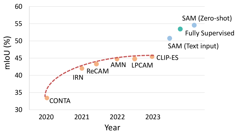
Figure 1: The performance of recent WSSS works (CONTA [87], IRN [1], ReCAM [12], AMN [41], LPCAM [11], and CLIP-ES [51]) and an evaluation of foundation models on MS COCO [50] val set.

We compare the performance of the traditional methods and foundation models on the MS COCO [50] validation set. As shown in Figure 1, the traditional methods reach a noticeable plateau in performance and the introduction of SAM has significantly enhanced the performance outcomes. In Section 5, we provide a comprehensive performance comparison of traditional methods and foundation models, offering insights into the potential and challenges of deploying foundational models in WSSS.

The paper is organized as below: Section 2 introduces the preliminaries for the WSSS task. Section 3 introduces the traditional models in WSSS. Section 4 introduces the applicability of visual foundation models in WSSS. Section 5 provides a comprehensive comparison of the performance of the traditional models and the application of foundation models. We conclude in Section 6.

2 Preliminaries

2.1 Problem Statement

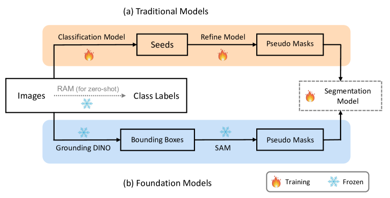
Figure 2: The pipeline of traditional methods and foundation models in WSSS. The dashed line means an optional step.

Fig. 2 illustrates the general pipeline for WSSS with image-level class labels for both traditional and foundation models. As shown in Fig. 2 (a), the traditional process begins with the training of a multi-label classification model using training images annotated with image-level class labels. Following this, we infer the class-specific seed areas for each image through the application of the Class Activation Map (CAM)[94] to the classification model. This results in a set of preliminary masks that undergo further refinement to produce the final pseudo masks. These pseudo masks then serve as the pseudo ground truth, enabling the training of a conventional fully supervised semantic segmentation model (e.g., DeepLabV2 [8]).

Fig. 2 (b) shows the pipeline of applying foundation models in WSSS. Given the images and their class labels, we first leverage Grounding DINO [53] to generate bounding boxes using text prompts. Then, we feed these bounding boxes into SAM to produce corresponding segmentation masks. Similar to the traditional methods, we can train a fully supervised semantic segmentation model using the produced masks. In another setting, when class labels for images are absent, RAM [90] can be deployed to produce tags for the images. Following this, the aforementioned pipeline can be applied to generate masks. Notably, there’s no need to train a fully supervised segmentation model in this context, as masks can be predicted without class labels.

2.2 Class Activation Map (CAM)

Class Activation Map (CAM) [94] is a simple yet effective technique employed to identify the regions within an image that a CNN leverages to identify a specific class present in that image. It is calculated by multiplying the classifier weights with the image features. The specifics of how CAM is computed will be discussed in the subsequent discussion.

In the multi-label classification model, Global Average Pooling (GAP) is utilized, followed by a prediction layer. To compute the prediction loss on each training example, the Binary Cross-Entropy (BCE) function is employed, as detailed in the following formula:

$$\mathcal{L}_{bce}=-\frac{1}{K}\sum_{k=1}^{K}y\left[k\right]\log\sigma\left(z[k]\right)+\left(1-y[k]\right)\log\left[1-\sigma\left(z[k]\right)\right],$$ (1)

where $z[k]$ denotes the prediction logit of the $k$-th class, $\sigma(\cdot)$ is the sigmoid function, and $K$ is the total number of foreground object classes (in the dataset). $y[k]\in\{0,1\}$ is the image-level label for the $k$-th class, where 1 denotes the class is present in the image and 0 otherwise. Once the classification model converges, we feed the image $\bm{x}$ into it to extract the CAM of class $k$ appearing in $\bm{x}$:

$$\operatorname{CAM}_{k}(\bm{x})=\frac{\operatorname{ReLU}\left(\bm{A}_{k}\right)}{\max\left(\operatorname{ReLU}\left(\bm{A}_{k}\right)\right)},\bm{A}_{k}=\mathbf{w}_{k}^{\top}f(\bm{x}),$$ (2)

where $\mathbf{w}_{k}$ denotes the classification weights (e.g., the FC layer of a ResNet) corresponding to the $k$-th class, and $f(\bm{x})$ represents the feature maps of $\bm{x}$ before the GAP.

As we mentioned in Section 1, CAM often struggles to capture the complete object, instead focusing on the most distinctive parts. As such, a significant portion of the works in WSSS aim to tackle this issue, endeavoring to produce more complete CAMs.

2.3 Related Works

To the best of our knowledge, there are only a few related survey papers [6, 66] on WSSS. Chan et al.[6] focused on evaluating state-of-the-art weakly-supervised semantic segmentation methods (up until 2019) across diverse datasets, including those for natural scenes, histopathology, and satellite images. Shen et al.[66] provided a comprehensive review of label-efficient segmentation methods. They established a taxonomy classifying these methods based on the level of supervision, varying from no supervision to coarse, incomplete, and noisy supervision. Furthermore, they considered different types of segmentation problems like semantic segmentation, instance segmentation, and panoptic segmentation. In their work, WSSS methods (up until 2021) that utilize image-level class labels fall under the coarse supervision category, further subdivided into six distinct parts (i.e., seed area refinement by cross-label constraint, seed area refinement by cross-pixel similarity, seed area refinement by cross-view consistency, seed area refinement by cross-image relation, pseudo mask generation by cross-pixel similarity, and pseudo mask generation by cross-image relation).

In comparison, our paper offers a novel perspective by proposing a new taxonomy to categorize traditional WSSS methods with image-level class labels. We also take a step further by exploring the applicability and effectiveness of recent foundation models in the WSSS context, providing up-to-date insights into this rapidly developing field.

3 Traditional Models

Traditional WSSS methods [75, 2, 1, 38, 74, 36, 12, 11] predominantly employ convolutional neural networks (CNNs) [23, 78]. Recently, Vision Transformer (ViT)[17] has recently emerged as a competitive alternative, achieving impressive results across multiple vision tasks [68, 72, 55, 4]. In fact, when pre-trained on extensive datasets, ViT can even surpass the state-of-the-art performance of CNNs. This indicates that, similar to their success in natural language processing, Transformers can be a powerful tool in computer vision. ViT-based WSSS methods [83, 62, 51, 63] also achieve competitive results in WSSS.

Most of the CNN-based and ViT-based methods are built upon CAM and developed to address the partial activation problem in CAM (as introduced in Section 1). We categorize those methods into four groups based on their operational level: pixel-wise, image-wise, cross-image, and external data.

3.1 Pixel-Wise Methods

In WSSS, even though we are limited to image-level labels, several methods delve into information at the pixel level. Some methods, such as  [41, 76, 43], derive pixel-level supervision signals from the image-level labels and then utilize them to optimize the pixel-wise loss functions. Others, like [2, 1, 82, 62, 29], explore the similarity among neighboring pixels. Expanding beyond individual pixels, certain approaches[27, 88, 59] harness the complementary information from local patches comprised of multiple pixels. Furthermore, there are other methods that explore contrastive learning [18, 63], graph convolution network [84] on the pixel level.

3.1.1 Pixel-wise loss

In WSSS with image-level class labels, we lack pixel-level labels for direct network supervision. As a result, certain methods have been developed to generate pixel-level supervision using diverse strategies. A straightforward strategy is to utilize the seed (or refined with dense Conditional Random Field (dCRF) [32]) as noisy supervisory. AMN [41] strives to increase the activation gap between the foreground and background regions. This ensures the resultant pseudo masks are robust to the global threshold values utilized to separate the foreground and background. To achieve this, AMN develops an activation manipulation network equipped with a per-pixel classification loss function (balanced cross-entropy loss [25]), which is supervised by the confident regions within the refined seeds. SANCE [43] trains a model to predict both object contour map and segmentation map, supervised by noisy seeds and online label simultaneously. This method employs noisy seeds as supervision for the segmentation branch and then refines the segmentation map to generate online labels to offer more accurate semantic supervision to the contour branch. Finally, they can generate more complete pseudo masks based on the segmentation map and the contour map. In Spatial-BCE [76], the authors highlighted a drawback of the traditional BCE loss function: it calculates the average over the entire probability map (i.e., via global average pooling), thereby causing all pixels to be optimized in the same direction. This process reduces the discriminative ability between the foreground and background pixels. To address this issue, they proposed a spatial BCE loss function that optimizes foreground and background pixels in distinct directions. An adaptive threshold is employed to divide the foreground and background within the initial seeds.

All three approaches share a crucial commonality: the use of a threshold to discern between foreground and background. This threshold stands as a pivotal determinant, given that it classifies each pixel as either background or foreground, thereby profoundly affecting the subsequent learning trajectory. The first two methods [41, 43] employ a fixed threshold, set as a hyper-parameter. In contrast, the latter approach [76] opts for a learnable threshold which can be optimized in the training process.

3.1.2 Pixel similarity

These kinds of methods leverage the similarity between adjacent pixels to refine seeds. PSA [2], IRN [1], AuxSegNet [82], AFA [62] propagate the object regions in the seed to semantically similar pixels in the neighborhood. It is achieved by the random walk [57] on a transition matrix where each element is an affinity score. PSA [2] incorporates an AffinityNet to predict semantic affinities between adjacent pixels, while IRN [1] includes an inter-pixel relation network to estimate class boundary maps based on which it computes affinities. AuxSegNet [82] integrates non-local self-attention blocks, which capture the semantic correlations of spatial positions based on the similarities between the feature vectors of any two positions.

The propagation of CAM in those methods can effectively reduce the false negatives in the original CAM. However, one potential limitation is that the random walk on transition matrix can be time-intensive.

Different from them, AFA [62] and SAS [29] leverage the pixel similarity from the inherent self-attention in the Transformer-based backbone. Specifically, Ru et al. [62] introduce an Affinity from Attention (AFA) module to learn semantic affinities from the multi-head self-attention (MHSA) in Transformers. Specifically, they generate an initial CAM and then use it to compute pseudo affinity labels, representing pixel similarity. These pseudo affinity labels are subsequently utilized to guide the affinity prediction made by the MHSA. Kim et al. [29] proposed a superpixel discovery method to find the semantic-aware superpixels based on the pixel-level feature similarity produced by self-supervised vision transformer [5]. Then the superpixels are utilized to expand the initial seed.

3.1.3 Local patch

Moving beyond the scope of a single pixel, certain methods operate within the context of a small patch composed of a cluster of adjacent pixels. CPN [88] demonstrates that the self-information of the CAM of an image is less than or equal to the sum of the self-information of the CAMs, which are obtained by complementary patch pair. They split an image into two images with complementary patch regions and used the sum of CAMs generated by the two images to mine out more foreground regions. L2G [27] employs a local classification network to extract attention from various randomly cropped local patches within the input image. Concurrently, it uses a global network to learn complementary attention knowledge across multiple local attention maps online.

Different from CPN [88] and L2G [27], where the patches are randomly divided, RPIM [59] utilizes the superpixel approach to partition the input images into different regions. It then uses an inter-region spreading module to discover the relationship between different regions and merge the regions that belong to the same object into a whole semantic region.

3.1.4 Other pixel-wise methods

Other methods operate at the pixel level but do not align squarely with the aforementioned categories. Fan et al. [20] proposed an intra-class discriminator (ICD) that is dedicated to separating the foreground and the background pixels within each image-level class. Such an intra-class discriminator is similar to a binary classifier for each image-level class, which identifies between the foreground pixels and the background pixels. NSROM [84] performs the graph-based global reasoning [64] on pixel-level feature maps to strengthen the classification network’s ability to capture global relations among disjoint and distant regions. This helps the network activate the object features outside the salient area. DRS [28] takes a unique approach by attempting to suppress the discriminative regions, thereby redirecting attention to adjacent non-discriminative regions. This is accomplished by introducing suppression controllers (which can be either learnable or non-learnable) to each layer of the CNNs, controlling the extent to which the attention is focused on discriminative regions. Specifically, any activation values that exceed a certain threshold (which can be fixed or learnable) multiplied by the maximum activation values will be suppressed to the maximum activation values. This methodology ensures that the model’s focus is more evenly distributed across the whole image, rather than being concentrated solely on the most distinctive regions. PPC [18] is instantiated with a unified pixel-to-prototype contrastive learning formulation, which shapes the pixel embedding space through a prototype-based metric learning methodology. The core idea is pulling pixels together to their positive prototypes and pushing them away from their negative prototypes to learn discriminative dense visual representations. ToCo [63] devises a Class Token Contrast (CTC) module inspired by the capability of ViT’s class tokens to capture high-level semantics. CTC uses reliable foreground and background regions within the initial CAM to derive positive and negative local images. The class tokens of these local images are then projected and contrasted with the global class token using InfoNCE loss [58], aiding in differentiating low-confidence regions within the CAM.

3.2 Image-Wise Methods

Image-wise methods are the most straightforward and have been the subject of numerous works. Researchers employing these methods have explored a diverse array of strategies. A considerable number of studies delve into adversarial learning [75, 34, 85, 71, 38, 35], context decoupling [87, 69, 81, 80], and consistency regularization [74, 10, 60]. Some tackle the problems of loss functions, introducing innovative solutions. Furthermore, several methods have emerged that focus on online attention accumulation [26], uncertainty estimation [47], and evaluating CAM’s coefficient of variation [48].

3.2.1 Adversarial learning

The first kind of method that leverages the idea of adversarial learning is adversarial erasing (AE) based methods. Wei et al. [75] proposed the first AE method, which discovers a small object region and erases the mined regions from the image. Then it feeds the image to the classification network again to drive the network to discover new and complementary object regions. Kweon et al. [34] proposed a class-specific AE framework that generates a class-specific mask for erasing by randomly sampling a single specific class to be erased (target class) among the existing classes on the image for obtaining more precise CAM.

Although AE methods expand the CAM by erasing the most discriminative regions, they often encounter high computation cost problem due to the multiple feed-forward process and the over-expansion problem due to the lack of guidance on when to stop the erasing process. To address this, the AEFT method  [85] reformulates the AE methods as a form of triplet learning. Specifically, it designates the original image as an anchor image, the masked high-confidence regions of the CAM on the anchor image as a positive image, and another image (which shares no class overlap with the anchor image) as a negative image. It aims to minimize the distance between the anchor and the positive image in the feature space while simultaneously maximizing the distance between the anchor and the negative image. As a result, when the CAMs are over-expanded, the embedding from the low-confidence region includes less information about the objects in the image, making it challenging for the network to differentiate this less informative embedding from the negative embedding. Consequently, the expansion of CAMs is intuitively suppressed. ECS-Net [71] investigates a way to provide additional supervision for the classification network by utilizing predictions of erased images. It first erases high-response regions from images and generates new CAMs of those erased images. Then, it samples reliable pixels from the new CAM and applies their segmentation predictions as semantic labels to train the corresponding original CAM. Instead of erasing multiple times, ECS-Net only needs to erase once, avoiding introducing excessive noise.

Instead of directly erasing the mined regions from the image, AdvCAM [38] perturbs the image along pixel gradients which increases the classification score of the target class. The result is that non-discriminative regions, which are nevertheless relevant to that class, gradually become involved in the CAM produced by the classification model. However, a notable drawback of AdvCAM is the computation of these gradients, which is computationally intensive and significantly slows down the process.

Unlike all those methods, kweon et al. [35] presented a framework that utilizes adversarial learning between a classifier and an image reconstructor. This method is inspired by the notion that no individual segment should be able to infer color or texture information from other segments if semantic segmentation is perfectly achieved. They introduced an image reconstruction task that aims to reconstruct one image segment from the remaining segments. The classifier is trained not only to classify the image but also to generate CAM that accurately segment the image, while contending with the reconstructor. In the end, the quality of the CAMs is enhanced by jointly training the classifier and the reconstructor in an adversarial manner.

3.2.2 Context decoupling

Some methods attempt to decouple the object from its surrounding context. For instance, Zhang et al. [87] proposed a structural causal model (CONTA) to analyze the causalities among images, their contexts, and class labels. Based on this, they developed a context adjustment method that eliminates confounding bias in the classification model, resulting in improved CAM. CDA [69] is a context decoupling augmentation technique that modifies the inherent context in which objects appear, thereby encouraging the network to remove reliance on the correlation between object instances and contextual information. Specifically, in the first stage, it uses the off-the-shelf WSSS methods to obtain basic object instances with high-quality segmentation. In the second, these object instances are randomly embedded into raw images to form the new input images. These images then undergo online data augmentation training in a pairwise manner with the original input images. Unlike CDA, which relies on pre-existing WSSS methods to separate background and foreground, BDM [81] utilizes saliency maps to generate a binary mask, cropping out images containing only the background or foreground for a given image. It subsequently applies consistency regularization to the CAMs derived from object instances seen in various scenes, thereby providing self-supervision for network training. Different from CDA and BDM, which apply a mask on the original image to decouple the foreground and background. Xie et al. [80] generates a class-agnostic activation map and disentangles image representation into the foreground and background representation. The disentangled representation are then used to create positive pairs (either foreground-foreground representation or background-background representation) and negative pairs (foreground-background representation) across a group of images. Finally, using these constructed pairs, a contrastive loss function is applied to encourage the network to separate foreground and background effectively.

3.2.3 Consistency regularization

These methods leverage consistency regularization to guide network learning. SEAM [74] employs consistency regularization on predicted CAMs from various transformed images to provide self-supervision for network learning. Similarly, SIPE [10] ensures the consistency between the general CAM and the proposed Image-Specific Class Activation Map (IS-CAM), which is derived from image-specific prototypes. Qin et al. [60] proposed an activation modulation and re-calibration scheme that leverages a spotlight branch and a compensation branch to provide complementary and task-oriented CAMs. The spotlight branch denotes the fundamental classification network, while the compensation branch contains an attention modulation module to rearrange the distribution of feature importance from the channel-spatial sequential perspective to dig out the important but easily ignored regions. A consistency loss is employed between the CAMs produced by the two branches.

The consistency regularization term is a versatile component that can be integrated into various network designs, provided there are coherent features or CAMs available. Typically presented as an auxiliary loss function, it enhances the model’s robustness without adding significant computational demands. This makes it an attractive add-on for ensuring consistent feature representations across different stages of the model.

3.2.4 Loss function

Some methods investigate the existing problems associated with the BCE loss function used in classification models and propose new loss functions to mitigate these issues. For instance, Lee et al. [36] highlighted that the final layer of a deep neural network, activated by sigmoid or softmax activation functions, often leads to an information bottleneck. To counter this, they proposed a novel loss function that eliminates the final non-linear activation function in the classification model while also introducing a new pooling method that further promotes the transmission of information from non-discriminative regions to the classification task. Similarly, Chen et al. [12] identified a problem with the widespread use of BCE loss — it fails to enforce class-exclusive learning, often leading to confusion between similar classes. They proved the superiority of softmax cross-entropy (SCE) loss and suggested integrating SCE into the BCE-based model to reactivate the classification model. Specifically, they masked the class-specific CAM on the feature maps and applied SCE loss on the masked feature maps, thereby facilitating better class distinction.

Both methods identify shortcomings in the prevailing BCE loss, specifically addressing the information bottleneck problem [36] and the class-exclusive learning problem [12]. They each introduce new loss functions to tackle these specific issues. Recognizing the pivotal role that the loss function plays in network learning, both methods contribute substantially to performance enhancements.

3.2.5 Other image-wise methods

Other methods that operate at the image level do not conform precisely to the aforementioned categories. Jiang et al. [26] proposed an online attention accumulation (OAA) strategy that maintains a cumulative attention map for each target category in each training image to accumulate the discovered different object parts. So that the integral object regions can be gradually promoted as the training goes. EDAM [77] masks the class-specific CAM on the feature maps and learns separate classifiers for each class. As the region of background and irrelevant foreground objects are removed in the class-specific feature map, to some extent, the performance of classification can be improved. PMM [48] computes the coefficient of variation for each channel of CAMs and then refines CAMs via exponential functions with the coefficient of variation as the control coefficient. This operation smooths the CAMs and could alleviate the partial response problem introduced by the classification pipeline. URN [47] simulates noisy variations of response by scaling the prediction map multiple times for uncertainty estimation. The uncertainty is then used to weigh the segmentation loss to mitigate noisy supervision signals. ESOL [44] employs an Expansion and Shrinkage scheme based on the offset learning in the deformable convolution [15], to sequentially improve the recall and precision of the located object in the two respective stages. The Expansion stage aims to recover the entire object as much as possible, by sampling the exterior object regions beyond the most discriminative ones, to improve the recall of the located object regions. The Shrinkage stage excludes the false positive regions and thus further enhances the precision of the located object regions. Unlike traditional transformers that employ a single class token, MCTFormer [83] uses multiple class tokens to learn the interactions between these class tokens and the patch tokens. This allows the model to learn class-specific activation maps from the class-to-patch attention of various class tokens.

3.3 Cross-Image Methods

Moving beyond a single image, certain connections often exist between different images within a dataset. Some methods explore these connections, whether they occur pair-wise [70, 21, 54], group-wise [89, 46, 80], or even on a dataset-wise scale [7, 95, 11].

3.3.1 Pair-wise

Some methods focus on capturing pairwise relationships between images. For instance, MCIS [70] employs two neural co-attentions in its classifier to capture complementary semantic similarities and differences across images. Given a pair of training images, one co-attention forces the classifier to recognize the common semantics from co-attentive objects, while the other drives the classifier to identify the unique semantics from the rest, uncommon objects. This dual attention approach helps the classifier discover more object patterns and better ground semantics in image regions. Similarly, Fan et al. [21] proposed an end-to-end cross-image affinity module designed to gather supplementary information from related images. Specifically, it builds pixel-level affinities across different images, allowing incomplete regions to glean additional information from other images. This approach results in more comprehensive object region estimations and mitigates ambiguity. Lastly, MBMNet [54] utilizes a parameter-shared siamese encoder to encode the representation of paired images and models their feature representation with a bipartite graph. They find the maximum bipartite matching between the graph nodes to determine relevant feature points in two images, which are then used to enhance the corresponding representations.

3.3.2 Group-wise

Some methods attempt to model more complex relationships within a group of images. For instance, Group-WSSS [46] explicitly models semantic dependencies in a group of images to estimate more reliable pseudo masks. Specifically, they formulate the task within a graph neural network (GNN) [64], which operates on a group of images and explores their semantic relations for more effective representation learning. Additionally, Zhang et al. [89] introduced a heterogeneous graph neural network (HGNN) to model the heterogeneity of multi-granular semantics within a set of input images. The HGNN comprises two types of sub-graphs: an external graph and an internal graph. The external graph characterizes the relationships across different images, aiming to mine inter-image contexts. The internal graph, which is constructed for each image individually, is used to mine inter-class semantic dependencies within each individual image. Through heterogeneous graph learning, the network can develop a comprehensive understanding of object patterns, leading to more accurate semantic concept grounding.

In these methods, it is important to determine the number of images in a group. There’s a delicate balance between capturing meaningful semantic relationships and introducing noise by grouping images. Both approaches utilize groups of $4$ images. As the number of images increases, the benefits from additional semantic cues plateau, while the noise introduced can lead to a decline in performance.

3.3.3 Dataset-wise

Beyond a group of images, some methods delve into the semantic connections present in the entire dataset. Chang et al. [7] introduced a self-supervised task leveraging sub-category information. To be more specific, for each class, they perform clustering on all local features (features at each spatial pixel position in the feature maps) within that class to generate pseudo sub-category labels. They then construct a sub-category objective that assigns the network a more challenging classification task. Similarly, LPCAM [11] also performs clustering on local features. However, instead of creating a sub-category objective, LPCAM utilizes the clustering centers, also known as local prototypes, as a non-biased classifier to compute the CAM. Since these local prototypes contain rich local semantics like the “head”, “leg”, and “body” of a “sheep”, they are able to solve the problem that the weight of the classifier (which is used to compute the CAM) in the classification model only captures the most discriminative features of objects. Zhou et al. [95] proposed Regional Semantic Contrast and Aggregation (RCA) method for dataset-level relation learning. RCA uses a regional memory bank to store a wide array of object patterns that appear in the training data, offering strong support for exploring the dataset-level semantic structure. More specifically, the semantic contrast pushes the network to bring the embedding closer to the memory embedding of the same category while pushing away those of different categories. This contrastive property complements the classification objective for each individual image, thereby improving object representation learning. On the other hand, semantic aggregation enables the model to gather dataset-level contextual knowledge, resulting in more meaningful object representations. This is achieved through a non-parametric attention module which summarizes memory representations for each image independently.

Compared to the pair-wise and group-wise methods, the dataset-wise methods can leverage more information from the whole dataset. These methods explore the object patterns on the whole dataset. These patterns are then captured and stored using mechanisms like “sub-category labels” [7], “local prototypes” [11], or “memory banks” [95], which can be later leveraged for model learning or CAM generation. These object patterns can effectively improve the CAM quality. Similar to group-wise methods, one challenge is the balance of meaningful semantic cues and potential noise. Thus, it always needs some operations, like selecting prototypes in LPCAM [11], to preserve useful object patterns and filter out noise.

3.4 Methods with External data

In addition to leveraging information within the dataset, some methods further employ external data resources to improve the classification model. These external resources can provide additional, diverse, and complementary information not present in the original dataset, helping to improve the model’s overall performance.

3.4.1 Saliency map

Saliency detection methods [52, 24, 91] generate saliency maps that distinguish between the foreground and the background in an image. Many WSSS methods [77, 37, 26, 25, 70, 95] exploit saliency maps as a post-processing step to refine the initial CAMs. Beyond their usage in post-processing, some methods employ saliency maps to aid model learning. For instance, both SSNet [86] and EPS [42] directly model the connection between saliency detection and WSSS. They minimize a saliency loss, which is defined as the pixel-wise difference between the actual saliency map and the estimated saliency map. However, the strategies they employ to estimate the saliency map of the input image differ. SSNet [86] uses a segmentation network to predict a pixel-level mask for each class and then aggregates the masks to create a saliency map. In contrast, EPS [42] designs a classifier to predict $C+1$ classes, consisting of $C$ target classes and one background class. They use $C$ foreground activation maps and the background activation map to estimate the saliency map.

These methods leverage a saliency detection model to generate the saliency maps, eliminating the need for extra human effort to annotate. However, there’s no guarantee that the saliency maps they produce will be perfect. Consequently, inaccuracies in the saliency maps can impact the overall performance of the method.

3.4.2 Out-of-Distribution data

Lee et al. [39] proposed to use Out-of-Distribution (OoD) data to address the issue of spurious correlation between foreground and background cues (e.g., “train” and “rail”). They collected their candidate OoD data, which do not include any foreground classes of interest, from another vision dataset OpenImages [33]. Taking the class “train” as an example, they initially select images in which the classification model’s predicted probability for “train” exceeded 0.5. They then manually filter out images that contained a “train”. The remaining images, which do not contain a ”train” but have a high predicted probability for the class ”train” in the classification model, can be used as out-of-distribution data. They assign out-of-distribution data with zero-vector labels (zero for all classes) and apply the common binary cross-entropy (BCE) loss for both in-distribution and out-of-distribution samples. The OoD data helps the model distinguish between in-distribution and out-of-distribution samples, thereby reducing false positive predictions in CAM.

Utilizing OoD data can significantly enhance the model’s ability to distinguish between objects and co-occurring background cues. However, the annotation of OoD data requires additional human effort.

4 Foundation Models

4.1 Contrastive Language-Image Pre-Training

Contrastive Language-Image Pre-Training (CLIP) [61] is designed to efficiently learn visual concepts from natural language supervision. The main innovation of CLIP is its use of a contrastive objective function, which is based on the principle that semantically similar inputs should be mapped to nearby points in the feature space, while semantically dissimilar inputs should be mapped to distant points. Specifically, CLIP is trained on a large dataset of image-text pairs using a contrastive loss that encourages the model to learn to map similar image and text representations close together in a joint feature space while pushing dissimilar representations apart.

CLIP has emerged as a powerful tool due to its ability to associate much wider visual concepts in the image with their text labels in an open-world setting. Two works have harnessed the potential of CLIP in WSSS. CLIMS [79] utilizes the CLIP model as a text-driven evaluator. Specifically, it employs a CNN to generate initial CAMs and applies the CAMs (or reversed CAMs) on the image as masks to identify the object (or background) regions. It then leverages object text prompts (e.g., “a photo of a train”) and class-related background text prompts (e.g., “a photo of railroad” for class “train”) to compute matching losses with the masked object and background regions, respectively. These losses work to ensure both the correctness and completeness of the initial CAMs. Different from CLIMS [79], Lin et al.[51] investigated the ability of CLIP to localize different categories through only image-level labels without any additional training. To efficiently generate high-quality segmentation masks from CLIP, they propose a framework with special designs for CLIP. They introduce the softmax function into GradCAM [65] and define a class-related background set to enforce mutual exclusivity among categories, thus suppressing the confusion caused by non-target classes and backgrounds. Meanwhile, to take full advantage of CLIP, they re-explore text inputs under the WSSS setting and customize two text-driven strategies: sharpness-based prompt selection and synonym fusion. The results show that the CLIP-based framework can efficiently generate pseudo masks for semantic segmentation without further training and outperforms most traditional WSSS methods.

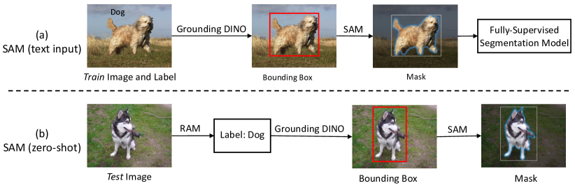
Figure 3: The pipeline of applying SAM in WSSS. All models except the fully-supervised segmentation model are kept frozen.

4.2 Segment Anything Model (SAM)

The Segment Anything Model (SAM) [30] is a recent image segmentation model exhibiting superior performance across various segmentation tasks. Different from the traditional semantic segmentation model [9, 92, 68] where the input is an image and the output is a mask, SAM introduces a new promptable segmentation task that supports various types of prompts, such as points, bounding boxes, and textual descriptions. It leverages a Transformer model [17] trained on the extensive SA-1B dataset (comprising over 1 billion masks derived from 11 million images), which gives it the ability to handle a wide range of scenes and objects. SAM is remarkable for its capability to interpret diverse prompts and successively generate various object masks. We investigate two settings to apply SAM in WSSS: text input (leveraging the class labels available for the train images in WSSS) and zero-shot (employed when only test data is available, given the absence of class labels for the val and test images in WSSS). The pipeline of the two settings is shown in Figure 3.

4.2.1 SAM (text input)

We follow the general pipeline in traditional methods (as shown in Figure 2) to generate pseudo masks first and then train the fully supervised semantic segmentation model (DeepLabV2 [8]). To generate pseudo masks, we consider feeding image and text prompts (class labels) as inputs to SAM. However, the text prompt functionality of SAM is not currently open-sourced. To circumvent this limitation, as shown in Figure 3 (a), we utilize Grounded-SAM  in our experiments for WSSS. Grounded-SAM is a hybrid of Grounding DINO [53] and SAM [30], enabling the grounding and segmentation of objects via text inputs. In particular, Grounding DINO can generate grounded bounding boxes using text prompts. Following this step, we feed these grounded bounding boxes into SAM to produce corresponding segmentation masks. The pipeline of SAM (text input) is summarized as follows:

• Step 1: Feed the train images and image-level class labels to Grounding DINO [53] to generate bounding boxes.

• Step 2: Feed the train images and generated bounding boxes to SAM [30] to generate masks.

• Step 3: Train the fully-supervised segmentation model (e.g. DeepLabV2 [8]) using the train images and generated masks.

• Step 4: Feed the test images to segmentation model to generate masks.

4.2.2 SAM (zero-shot)

Different from the general pipeline (as shown in Figure 2) used in traditional WSSS, we also endeavor to directly assess SAM’s performance on the val and test images, which lack any text inputs. As illustrated in Figure 3 (b), we utilize the image tagging model, Recognize Anything Model (RAM) [90], to identify the objects within the image first. RAM is a strong foundation model designed for image tagging. It demonstrates the strong zero-shot ability to recognize any category with high accuracy, surpassing the performance of both fully supervised models and existing generalist approaches like CLIP [61] and BLIP [45]. With the recognized category label, we adhere to the similar pipeline as SAM (text input). The pipeline of SAM (zero-shot) is summarized as follows:

• Step 1: Feed the test images to RAM [90] to generate tags.

• Step 2: Feed the test images and generated tags to Grounding DINO [53] to generate bounding boxes.

• Step 3: Feed the test images and generated bounding boxes to SAM [30] to generate masks.

Compared to SAM (text input), SAM (zero-shot) incorporates an additional model (SAM) to identify objects within the image. Notably, the SAM (zero-shot) method eliminates the need for train images and circumvents the requirement to train a fully supervised segmentation model in SAM (text input). This is because SAM (zero-shot) can predict masks even in the absence of class labels.

5 Methodological Comparison

In this section, we provide a comprehensive comparison between the traditional models introduced in Section 3 and the application of foundation models introduced in Section 4. We also offer insights into the potential and challenges of deploying foundational models in WSSS.

5.1 Evaluation Protocol

Datasets. There are two benchmark datasets in WSSS: PASCAL VOC 2012 [19] and MS COCO 2014 [50]. PASCAL VOC 2012 dataset contains $20$ foreground object categories and $1$ background category with $1,464$ train images, $1,449$ val images, and $1,456$ test images. All works use the enlarged training set with $10,582$ training images provided by SBD [22]. MS COCO 2014 dataset consists of $80$ foreground categories and $1$ background category, with $82,783$ and $40,504$ images in the train and val sets, respectively.

Metrics. There are two evaluation steps for WSSS — the pseudo mask quality and the semantic segmentation performance. The pseudo mask quality is evaluated by the mean Intersection-over-Union (mIoU) of the generated pseudo masks and the corresponding ground truth masks on the train images. In terms of the semantic segmentation performance, we evaluate the mIoU between the predicted masks and the corresponding ground truth masks on both the val and test images.

Implementation details. Regarding SAM (text input), we load the default pretrained Grounded-SAM model (Swin-T [55] for Gounding DINO [53] and ViT-H [17] for SAM [30]). After generating pseudo masks, we train the DeepLabV2 [8] with ImageNet [16] pretrained ResNet-101 [23]. In the SAM (zero-shot), we load the pre-trained RAM-14M [90] model based on Swin-T [55]. To align the tags from the RAM with the class labels in the VOC datasets, we establish a mapping strategy due to the different terminologies used by the models and datasets. Specifically, we consider “couch” from RAM to correspond with “sofa” in the VOC dataset, “plane” with “aeroplane”, “plant” with “potted plant”, and “monitor”, “screen”, and “television” with “TV monitor”. Additionally, we map “person”, “man”, “woman”, “boy”, “girl”, “child”, and “baby” tags from RAM to the “person” class in VOC. This strategy ensures comparable results between SAM and the ground truth annotations of the VOC dataset. On the MS COCO dataset, we adopt a similar strategy for aligning the RAM tags with the class labels. Due to the larger and more diverse range of classes in MS COCO, please refer to our provided code .

For the DeepLabV2 [8] in the step of fully supervised semantic segmentation, following [1, 36, 12], we crop each training image to the size of 321×321. We train the model for 20k and 100k iterations on VOC and MS COCO datasets, respectively, with the respective batch size of 5 and 10. The learning rate is set as 2.5e-4 and weight decay as 5e-4. Horizontal flipping and random crop are used for data augmentation.

Table 1: Comparison of the WSSS methods in terms of the pseudo mask mIou(%) and the segmentation mIoU results (%) using DeepLabV2 [8] on VOC [19] and MS COCO [50] dataset. “P.M.” denotes pseudo mask, “RN” denotes “ResNet”, and “WRN” denotes “WideResNet”.

	Methods	Venue	Backbone	Saliency	Segmentation		VOC			COCO		Row No.
					Backbone	Pretrain	P.M.	Val	Test	P.M.	Val
Pixel-Level	SANCE [43]	CVPR 22	RN-101		RN-101	ImageNet	-	70.9	72.2	-	44.7	1
	AMN [41]	CVPR 22	RN-50		RN-101	ImageNet	72.2	69.5	69.6	46.7	44.7	2
	Spatial-BCE [76]	ECCV 22	WRN-38		RN-101	ImageNet	70.4	70.0	71.3	-	35.2	3
	PSA [2]	CVPR 18	WRN-38		WRN-38	ImageNet	59.7	61.7	63.8	-	-	4
	IRN [1]	CVPR 19	RN-50		RN-101	ImageNet	66.5	63.5	64.8	42.4	42.0	5
	AuxSegNet [82]	ICCV 21	WRN-38	✓	WRN-38	ImageNet	-	69.0	68.6	-	33.9	6
	AFA [62]	CVPR 22	MiT-B1		MiT-B1	ImageNet	68.7	66.0	66.3	-	38.9	7
	SAS [29]	AAAI 23	ViT-B/8		RN-101	ImageNet	-	69.5	70.1	-	44.8	8
	CPN [88]	ICCV 21	WRN-38		WRN-38	ImageNet	-	67.8	68.5	-	-	9
	L2G [27]	CVPR 22	WRN-38	✓	RN-101	COCO	70.3	72.1	71.7	-	44.2	10
	RPIM [59]	ACMMM 22	WRN-38	✓	RN-101	COCO	69.3	71.4	71.4	-	-	11
	ICD [20]	CVPR 20	VGG-16		RN-101	ImageNet	-	64.1	64.3	-	-	12
	NSROM [84]	CVPR 21	RN-50		RN-101	ImageNet		68.3	68.5	-	-	13
	DRS [28]	AAAI 21	VGG-16	✓	RN-101	ImageNet	-	71.2	71.4	-	-	14
	PPC [18]+SEAM	CVPR 22	WRN-38		WRN-38	ImageNet	69.2	67.7	67.4	-	-	15
	PPC [18]+EPS	CVPR 22	WRN-38	✓	RN-101	ImageNet	73.3	72.6	73.6	-	-	16
	ToCo [63]	CVPR 23	ViT-B/16		ViT-B/16	ImageNet	72.2	69.8	70.5	-	41.3	17
Image-Level	AE [75]	CVPR 17	VGG-16		VGG-16	ImageNet	-	55.5	55.7	-	-	18
	CSE [34]	ICCV 21	WRN-38		WRN-38	ImageNet	-	68.4	68.2	-	36.4	19
	ECS-Net [71]	ICCV 21	WRN-38		WRN-38	ImageNet	-	66.6	67.6	-	-	20
	AdvCAM [38]	CVPR 21	RN-50		RN-101	ImageNet	70.5	68.1	68.0	-	-	21
	AEFT [85]	ECCV 22	WRN-38		WRN-38	ImageNet	71.0	70.9	71.7	-	44.8	22
	ACR [35]	CVPR 23	WRN-38		WRN-38	ImageNet	72.3	71.9	71.9	-	45.3	23
	CONTA [87]	NeurIPS 20	RN-50		RN-101	ImageNet	67.9	65.3	66.1	-	33.4	24
	CDA [69]	ICCV 21	RN-50		RN-101	ImageNet	67.7	65.8	66.4	-	33.7	25
	BDM [81]	ACMMM 22	WRN-38	✓	RN-101	ImageNet	72.3	71.0	71.0	-	36.7	26
	CCAM [80]	CVPR 22	WRN-38		WRN-38	ImageNet	65.5	-	-	-	-	27
	SEAM [74]	CVPR 20	WRN-38		WRN-38	ImageNet	-	64.5	64.7	-	-	28
	PMM [48]	ICCV 21	WRN-38		WRN-38	ImageNet	-	68.5	69.0	-	36.7	29
	AMR [60]	AAAI 22	RN-50		RN-101	ImageNet	69.7	68.8	69.1	-	-	30
	SIPE [10]	CVPR 22	RN-50		RN-101	ImageNet	68.8	68.8	69.7	-	40.6	31
	RIB [36]	NeurIPS 21	RN-50		RN-101	ImageNet	70.6	68.3	68.6	45.6	44.2	32
	ReCAM [12]	CVPR 22	RN-50		RN-101	ImageNet	70.9	68.5	68.4	44.1	42.9	33
	OOA [26]	ICCV 19	RN-101		RN-101	ImageNet	-	65.2	66.4	-	-	34
	EDAM [77]	CVPR 21	RN-50	✓	RN-101	COCO	68.1	70.9	71.8	-	-	35
	PMM [48]	ICCV 21	WRN-38		WRN-38	ImageNet	-	68.5	69.0	-	36.7	36
	URN [47]	AAAI 22	RN-101		RN-101	ImageNet	-	69.5	69.7	-	40.7	37
	ESOL [44]	NeurIPS 22	RN-50		RN-101	COCO	68.7	69.9	69.3	44.6	42.6	38
	MCTformer [83]	CVPR 22	DeiT-S		WRN-38	VOC	69.1	71.9	71.6	-	42.0	39
Cross-Image	MCIS [70]	ECCV 20	VGG-16		RN-101	ImageNet	-	66.2	66.9	-	-	40
	CIAN [21]	AAAI 20	RN-101		RN-101	ImageNet	-	64.3	65.3	-	-	41
	MBM-Net [54]	ACMMM 20	RN-50		RN-50	ImageNet	-	66.2	67.1	-	-	42
	Group-WSSS [46]	AAAI 21	RN-101		RN-101	ImageNet	-	68.2	68.5	-	-	43
	HGNN [89]	ACMMM 22	WRN-38	✓	RN-101	COCO	70.2	70.5	71.0	-	34.5	44
	SCE [7]	CVPR 20	WRN-38		RN-101	ImageNet	-	66.1	65.9	-	-	45
	RCA [95]+OOA	CVPR 22	WRN-38	✓	RN-101	ImageNet	73.2	71.1	71.6	-	35.7	46
	RCA [95]+EPS	CVPR 22	WRN-38	✓	RN-101	ImageNet	74.1	72.2	72.8	-	36.8	47
	LPCAM [11]	CVPR 23	RN-50		RN-101	ImageNet	71.2	68.6	68.7	46.8	44.5	48
External	SSNet [86]	ICCV 19	VGG-16	✓	VGG-16	ImageNet	-	63.3	64.3	-	-	49
	EPS [42]	CVPR 21	WRN-38	✓	RN-101	COCO	69.4	70.9	70.8	-	-	50
	OoD [39]+AdvCAM	CVPR 22	RN-50		RN-101	ImageNet	72.1	69.8	69.9	-	-	51
FMs	CLIMS [79]	CVPR 22	RN-50		RN-101	COCO	70.5	70.4	70.0	-	-	52
	CLIP-ES [51]	CVPR 23	ViT-B/16		RN-101	ImageNet	75.0	71.1	71.4	-	45.4	53
	SAM (text input)	-	-		RN-101	ImageNet	86.4	72.7	72.8	64.4	50.8	54
	SAM (zero-shot)	-	-		-	-	78.2	74.0	73.8	54.6	54.6	55
	Fully-Supervised	-	-		RN-101	ImageNet	100.0	75.3	75.6	100.0	53.5	56

5.2 Results of Traditional Models

Table 1 (Rows 1-51) presents the performance of the traditional WSSS methods on VOC and MS COCO datasets. To make a methodological comparison, we compile a summary of important factors such as the venue of the original research publication, the classification backbone used, whether the method utilizes a saliency map, the semantic segmentation backbone deployed, and the source of the pretrained parameters.

5.3 Evaluation of SAM

Quality of pseudo masks. Both SAM (text input) and SAM (zero-shot) demonstrate outstanding performance. As shown in Table 1, on the VOC dataset, SAM (text input) achieves a mIoU score of $86.4\%$ (Row 54), surpassing the state-of-the-art method CLIP-ES [51] by a significant margin of $11.4\%$ (Row 53). Similarly, on the MS COCO dataset, it outperforms the state-of-the-art method LPCAM [11] by an impressive margin of $17.6\%$ (Row 48). While SAM (zero-shot) (Row 55) may not perform quite as well as SAM (text input), it nevertheless outperforms the state-of-the-art traditional methods on both datasets.

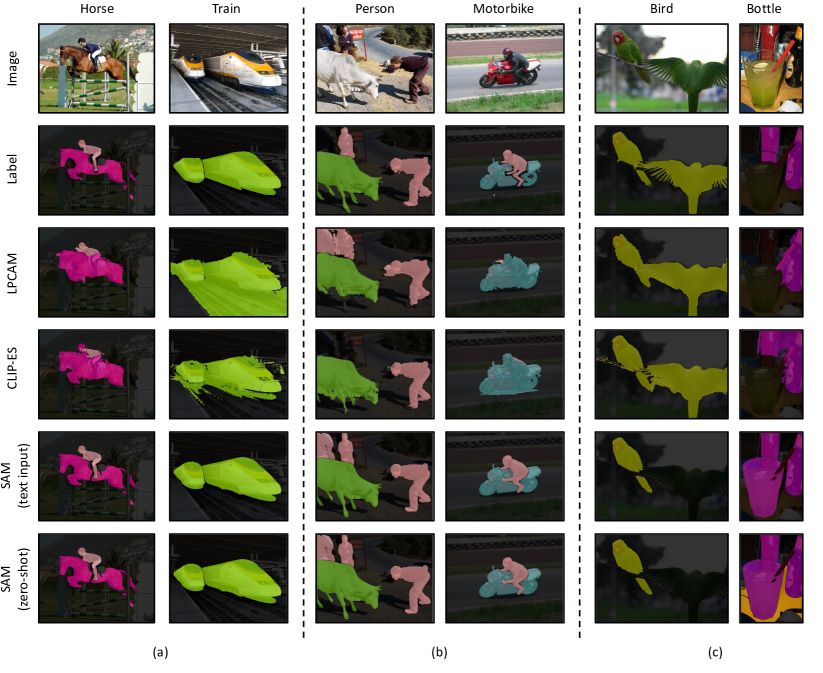
Figure 4: Visualization of pseudo masks generated by LPCAM [11], CLIP-ES [51], SAM (text input), and SAM (zero-shot) on VOC dataset. (a) Examples showcasing high-quality masks produced by both SAM (text input) and SAM (zero-shot). (b) Examples where SAM produced masks that even surpass the quality of the ground truth masks. (c) Examples illustrating the failure cases of SAM (text input) and SAM (zero-shot).

Semantic segmentation results of SAM (text input). SAM (text input) surpasses traditional methods and closely approaches the performance of the fully-supervised DeepLabV2 [8]. As shown in Table 1, on the VOC dataset, although SAM (text input) significantly outperforms CLIP-ES in terms of the quality of pseudo masks, their segmentation performance gap is only $1.6\%$ (Row 53 and 54) on the val and $1.4\%$ on test set. When compared with a fully-supervised method (considered as the upper bound), SAM (text input) remains competitive with a $2.6\%$ gap (Row 54 and Row 56) on the val set and $2.8\%$ on test set. This suggests that both CLIP-ES and SAM (text input) are capable of producing pseudo masks of sufficient quality to train the segmentation network effectively. Hence, further improvements in pseudo mask quality yield only marginal gains in segmentation performance. On the more challenging MS COCO dataset, we observe a more substantial gap. There is a $5.4\%$ performance difference (Row 53 and 54) between CLIP-ES and SAM (text input) on the val set, and a $2.7\%$ gap (Row 54 and 56) between SAM (text input) and the fully-supervised method. This could suggest that the increase in complexity and diversity in the MS COCO dataset makes it harder for WSSS methods to reach the performance level of fully-supervised methods.

Semantic segmentation results of SAM (zero-shot). We observe a significant gap in Row 54 between the pseudo mask on train set and the segmentation masks on val set and test set of SAM (text input). This suggests that the performance might be constrained by the fully-supervised DeepLabV2 [8] segmentation model. In the zero-shot setting, as shown in Table 1, the results indicate that SAM (zero-shot) outperforms SAM (text input) (as seen in Row 54 and 55) on both the val and test sets across both datasets. Furthermore, SAM (zero-shot) surpasses the fully-supervised DeepLabV2 model(as evident in the comparison between Rows 55 and 56) on the challenging MS COCO dataset, highlighting the strong capabilities of the foundation models for WSSS.

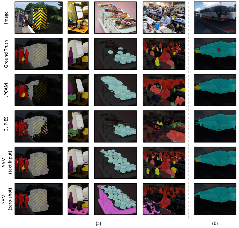
Figure 5: Visualization of pseudo masks generated by LPCAM [11], CLIP-ES [51], SAM (text input), and SAM (zero-shot) on MS COCO dataset. (a) Examples showcasing high-quality masks produced by SAM in complex scenes. (b) Examples illustrating the failure cases of SAM.

Table 2: Per-class pseudo mask quality (mIoU) of SAM (text input) and SAM (zero-shot) on VOC dataset. We classify the 20 classes in the VOC dataset into three categories: “animals”, “transportation”, and “objects/items”, with an additional class for “person”.

		Animals						Transportation							Objects/Items
	person	bird	cat	cow	dog	horse	sheep	aeroplane	bicycle	boat	bus	car	motorbike	train	bottle	chair	dining table	potted plant	sofa	TV monitor
Text input	90.0	94.3	94.5	94.8	91.1	93.9	97.4	96.8	65.2	89.6	90.2	86.5	84.1	96.1	91.0	73.8	48.9	73.8	78.4	88.9
Zero-shot	86.0	85.9	87.0	94.8	81.4	86.7	97.3	96.6	63.9	76.9	90.1	71.0	84.7	93.9	89.2	41.1	31.2	56.7	52.5	82.9

Qualitative result. Compared to the traditional method and CLIP-based method, as shown in Figure 4 (a) and (b), both SAM (text input) and SAM (zero-shot) show higher mask quality in terms of the clear boundaries not only between the background and foreground but also among different objects. In the example of “train”, SAM (text input) and SAM (zero-shot) successfully distinguish between “train” and “railroad”, a challenge that many WSSS methods struggle with due to the co-occurrence of these elements. But SAM (text input) and SAM (zero-shot) will also suffer from the false negative and false positive problem when the tagging model (RAM [90]) and grounding model (Grounding DINO [53]) wrongly tag or detect some objects. As shown in Figure 4 (c), SAM (text input) fails to identify a “bird” and mistakenly classifies a “cup” as a “bottle”. And SAM (zero-shot) wrongly recognizes a “dining table”. All these failures can be attributed to the grounding model or tagging model rather than SAM, suggesting that the capabilities of the grounding or tagging model could potentially limit the performance of SAM (text input). When compared to the human annotation, Figure 4 (b) highlights cases where SAM (text input) generates masks that even surpass the quality of human annotations. For instance, in the “person” example, the human annotation fails to include the person in the top left corner. In the “motorbike” example, SAM (text input) can produce precise boundaries in the overlapping scenarios. This suggests the strong capabilities of the foundation models in WSSS.

In complex scene examples from the MS COCO dataset, as illustrated in Figure 5 (a), both SAM (text input) and SAM (zero-shot) demonstrate their robust capability to annotate multiple smaller objects distinctly. For instance, in scenes with numerous “donuts” in close proximity, SAM can distinctly annotate each one, a proficiency similarly observed in the “person” example. Similar to the result on the VOC dataset, both SAM (text input) and SAM (zero-shot) also suffer from the false negative and false positive problem when the tagging model and grounding model wrongly tag or detect the objects. Figure 5 (b) shows a case where SAM (text input) fails to detect the “person” inside the “bus”, while SAM (zero-shot) overlooks the “car” near the “bus”. These failures can also be attributed to the grounding model or tagging model rather than SAM.

Per-class analysis. We investigate the per-class pseudo mask quality on the VOC dataset to examine the quality of pseudo masks produced by SAM (text input). As detailed in Table 2, SAM (text input) consistently generates high mIoU scores for most classes related to animals and transportation. However, it fares relatively poorer for classes related to objects or items. We believe that the observed differences could be due to the contrasting nature of the scenes where these subjects are usually found. Specifically, images of animals and transportation modes predominantly portray outdoor scenes, which generally have simpler backgrounds. In contrast, images of objects/items are frequently set indoors and are often characterized by more intricate backgrounds. Similarly, SAM (zero-shot) displays performance comparable to SAM (text input) in most classes associated with animals and transportation. However, there is a substantial gap when it comes to complex indoor scenes. This implies that the tagging model may encounter challenges in recognizing objects within complex indoor settings.

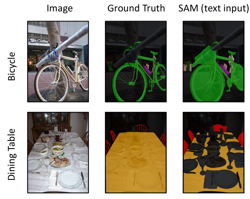
Figure 6: Examples (including images, ground truth labels, and pseudo masks produced by SAM (text input)) of bicycles and dining tables on VOC dataset.

Failure cases analysis. To delve deeper into the specifics, we turn our attention to the two categories with the lowest mIoU: bicycles and dining tables. As depicted in Fig. 6, the unique annotation protocols of the VOC dataset come to the fore. Notably, the dataset annotations exclude the hollow sections of bicycle wheels and encompass items present on dining tables. In contrast, the results from SAM (text input) manifest opposing tendencies. Consequently, it becomes clear that this observed deviation is not a flaw inherent to the model. Instead, it’s a discrepancy that emerges due to the differences in annotation strategies employed during the creation of the dataset. Hence, it’s essential to consider such factors when interpreting the performance of the model across different categories.

6 Conclusion

In this work, we embark on a deep exploration of weakly supervised semantic segmentation (WSSS) methods, and more specifically, the potential of using foundation models for this task. We first recapitulated the key traditional methods used in WSSS, outlining their principles and limitations. Then, we examine the potential of applying the Segment Anything Model (SAM) in WSSS, in two scenarios: text input and zero-shot.

Our results demonstrate that SAM (text input) and SAM (zero-shot) significantly outperform traditional methods in terms of pseudo mask quality. In some instances, they even approach or surpass the performance of fully supervised methods. These results highlight the immense potential of foundation models in WSSS. Our qualitative analysis further revealed that the quality of pseudo masks generated by our methods often exceeds the quality of human annotations, demonstrating their capability to produce high-quality segmentation masks. Our in-depth analysis brought to light some of the challenges in applying foundation models to WSSS. One such challenge is the discrepancy between the annotation strategies employed in the creation of the dataset and the models’ segmentation approach, leading to divergences in performance. Also, we observed that the complexity of the scenes and the diversity of the categories in datasets could affect the model’s performance.

Despite the considerable success of the SAM approach, several avenues for future research emerge from this work. First, further improvements could be made to the grounding and tagging models, which could potentially boost SAM’s performance. Second, the discrepancies identified between different annotation strategies suggest the necessity for a more standardized annotation protocol. Lastly, exploring the application of foundation models in WSSS in other more challenging datasets could provide insights into their generalizability and robustness across diverse scenarios. This research provides valuable insights into the WSSS task and highlights the promise of foundation models. We anticipate they will play an increasingly central role in advancing weakly supervised learning tasks.

Acknowledgments The author gratefully acknowledges the support of the A*STAR under its AME YIRG Grant (Project No.A20E6c0101).

References

- [1] Jiwoon Ahn, Sunghyun Cho, and Suha Kwak. Weakly supervised learning of instance segmentation with inter-pixel relations. In CVPR, pages 2209–2218, 2019.
- [2] Jiwoon Ahn and Suha Kwak. Learning pixel-level semantic affinity with image-level supervision for weakly supervised semantic segmentation. In CVPR, pages 4981–4990, 2018.
- [3] Tom Brown, Benjamin Mann, Nick Ryder, Melanie Subbiah, Jared D Kaplan, Prafulla Dhariwal, Arvind Neelakantan, Pranav Shyam, Girish Sastry, Amanda Askell, et al. Language models are few-shot learners. NeurIPS, 33:1877–1901, 2020.
- [4] Nicolas Carion, Francisco Massa, Gabriel Synnaeve, Nicolas Usunier, Alexander Kirillov, and Sergey Zagoruyko. End-to-end object detection with transformers. In ECCV, pages 213–229, 2020.
- [5] Mathilde Caron, Hugo Touvron, Ishan Misra, Hervé Jégou, Julien Mairal, Piotr Bojanowski, and Armand Joulin. Emerging properties in self-supervised vision transformers. In ICCV, pages 9650–9660, 2021.
- [6] Lyndon Chan, Mahdi S Hosseini, and Konstantinos N Plataniotis. A comprehensive analysis of weakly-supervised semantic segmentation in different image domains. IJCV, 129:361–384, 2021.
- [7] Yu-Ting Chang, Qiaosong Wang, Wei-Chih Hung, Robinson Piramuthu, Yi-Hsuan Tsai, and Ming-Hsuan Yang. Weakly-supervised semantic segmentation via sub-category exploration. In CVPR, pages 8991–9000, 2020.
- [8] Liang-Chieh Chen, George Papandreou, Iasonas Kokkinos, Kevin Murphy, and Alan L Yuille. Deeplab: Semantic image segmentation with deep convolutional nets, atrous convolution, and fully connected crfs. TPAMI, 40(4):834–848, 2017.
- [9] Liang-Chieh Chen, Yukun Zhu, George Papandreou, Florian Schroff, and Hartwig Adam. Encoder-decoder with atrous separable convolution for semantic image segmentation. In ECCV, pages 801–818, 2018.
- [10] Qi Chen, Lingxiao Yang, Jianhuang Lai, and Xiaohua Xie. Self-supervised image-specific prototype exploration for weakly supervised semantic segmentation. In CVPR, 2022.
- [11] Zhaozheng Chen and Qianru Sun. Extracting class activation maps from non-discriminative features as well. In CVPR, pages 3135–3144, 2023.
- [12] Zhaozheng Chen, Tan Wang, Xiongwei Wu, Xian-Sheng Hua, Hanwang Zhang, and Qianru Sun. Class re-activation maps for weakly-supervised semantic segmentation. In CVPR, pages 969–978, 2022.
- [13] Marius Cordts, Mohamed Omran, Sebastian Ramos, Timo Rehfeld, Markus Enzweiler, Rodrigo Benenson, Uwe Franke, Stefan Roth, and Bernt Schiele. The cityscapes dataset for semantic urban scene understanding. In CVPR, pages 3213–3223, 2016.
- [14] Jifeng Dai, Kaiming He, and Jian Sun. Boxsup: Exploiting bounding boxes to supervise convolutional networks for semantic segmentation. In ICCV, pages 1635–1643, 2015.
- [15] Jifeng Dai, Haozhi Qi, Yuwen Xiong, Yi Li, Guodong Zhang, Han Hu, and Yichen Wei. Deformable convolutional networks. In ICCV, pages 764–773, 2017.
- [16] Jia Deng, Wei Dong, Richard Socher, Li-Jia Li, Kai Li, and Li Fei-Fei. Imagenet: A large-scale hierarchical image database. In CVPR, pages 248–255, 2009.
- [17] Alexey Dosovitskiy, Lucas Beyer, Alexander Kolesnikov, Dirk Weissenborn, Xiaohua Zhai, Thomas Unterthiner, Mostafa Dehghani, Matthias Minderer, Georg Heigold, Sylvain Gelly, et al. An image is worth 16x16 words: Transformers for image recognition at scale. In ICLR, 2021.
- [18] Ye Du, Zehua Fu, Qingjie Liu, and Yunhong Wang. Weakly supervised semantic segmentation by pixel-to-prototype contrast. In CVPR, pages 4320–4329, 2022.
- [19] Mark Everingham, Luc Van Gool, Christopher KI Williams, John Winn, and Andrew Zisserman. The pascal visual object classes (voc) challenge. IJCV, 88(2):303–338, 2010.
- [20] Junsong Fan, Zhaoxiang Zhang, Chunfeng Song, and Tieniu Tan. Learning integral objects with intra-class discriminator for weakly-supervised semantic segmentation. In CVPR, pages 4283–4292, 2020.
- [21] Junsong Fan, Zhaoxiang Zhang, Tieniu Tan, Chunfeng Song, and Jun Xiao. Cian: Cross-image affinity net for weakly supervised semantic segmentation. In AAAI, volume 34, pages 10762–10769, 2020.
- [22] Bharath Hariharan, Pablo Arbeláez, Lubomir Bourdev, Subhransu Maji, and Jitendra Malik. Semantic contours from inverse detectors. In ICCV, pages 991–998, 2011.
- [23] Kaiming He, Xiangyu Zhang, Shaoqing Ren, and Jian Sun. Deep residual learning for image recognition. In CVPR, pages 770–778, 2016.
- [24] Qibin Hou, Ming-Ming Cheng, Xiaowei Hu, Ali Borji, Zhuowen Tu, and Philip HS Torr. Deeply supervised salient object detection with short connections. In CVPR, pages 3203–3212, 2017.
- [25] Zilong Huang, Xinggang Wang, Jiasi Wang, Wenyu Liu, and Jingdong Wang. Weakly-supervised semantic segmentation network with deep seeded region growing. In CVPR, pages 7014–7023, 2018.
- [26] Peng-Tao Jiang, Qibin Hou, Yang Cao, Ming-Ming Cheng, Yunchao Wei, and Hong-Kai Xiong. Integral object mining via online attention accumulation. In ICCV, pages 2070–2079, 2019.
- [27] Peng-Tao Jiang, Yuqi Yang, Qibin Hou, and Yunchao Wei. L2g: A simple local-to-global knowledge transfer framework for weakly supervised semantic segmentation. In CVPR, 2022.
- [28] Beomyoung Kim, Sangeun Han, and Junmo Kim. Discriminative region suppression for weakly-supervised semantic segmentation. In AAAI, volume 35, pages 1754–1761, 2021.
- [29] Sangtae Kim, Daeyoung Park, and Byonghyo Shim. Semantic-aware superpixel for weakly supervised semantic segmentation. In AAAI, volume 37, pages 1142–1150, 2023.
- [30] Alexander Kirillov, Eric Mintun, Nikhila Ravi, Hanzi Mao, Chloe Rolland, Laura Gustafson, Tete Xiao, Spencer Whitehead, Alexander C Berg, Wan-Yen Lo, et al. Segment anything. arXiv preprint arXiv:2304.02643, 2023.
- [31] Alexander Kolesnikov and Christoph H Lampert. Seed, expand and constrain: Three principles for weakly-supervised image segmentation. In ECCV, pages 695–711, 2016.
- [32] Philipp Krähenbühl and Vladlen Koltun. Efficient inference in fully connected crfs with gaussian edge potentials. NeurIPS, 24, 2011.
- [33] Alina Kuznetsova, Hassan Rom, Neil Alldrin, Jasper Uijlings, Ivan Krasin, Jordi Pont-Tuset, Shahab Kamali, Stefan Popov, Matteo Malloci, Alexander Kolesnikov, et al. The open images dataset v4: Unified image classification, object detection, and visual relationship detection at scale. IJCV, 128(7):1956–1981, 2020.
- [34] Hyeokjun Kweon, Sung-Hoon Yoon, Hyeonseong Kim, Daehee Park, and Kuk-Jin Yoon. Unlocking the potential of ordinary classifier: Class-specific adversarial erasing framework for weakly supervised semantic segmentation. In ICCV, pages 6994–7003, 2021.
- [35] Hyeokjun Kweon, Sung-Hoon Yoon, and Kuk-Jin Yoon. Weakly supervised semantic segmentation via adversarial learning of classifier and reconstructor. In CVPR, pages 11329–11339, 2023.
- [36] Jungbeom Lee, Jooyoung Choi, Jisoo Mok, and Sungroh Yoon. Reducing information bottleneck for weakly supervised semantic segmentation. In NeurIPS, pages 27408–27421, 2021.
- [37] Jungbeom Lee, Eunji Kim, Sungmin Lee, Jangho Lee, and Sungroh Yoon. Ficklenet: Weakly and semi-supervised semantic image segmentation using stochastic inference. In CVPR, pages 5267–5276, 2019.
- [38] Jungbeom Lee, Eunji Kim, and Sungroh Yoon. Anti-adversarially manipulated attributions for weakly and semi-supervised semantic segmentation. In CVPR, pages 4071–4080, 2021.
- [39] Jungbeom Lee, Seong Joon Oh, Sangdoo Yun, Junsuk Choe, Eunji Kim, and Sungroh Yoon. Weakly supervised semantic segmentation using out-of-distribution data. In CVPR, 2022.
- [40] Jungbeom Lee, Jihun Yi, Chaehun Shin, and Sungroh Yoon. Bbam: Bounding box attribution map for weakly supervised semantic and instance segmentation. In CVPR, pages 2643–2652, June 2021.
- [41] Minhyun Lee, Dongseob Kim, and Hyunjung Shim. Threshold matters in wsss: Manipulating the activation for the robust and accurate segmentation model against thresholds. In CVPR, 2022.
- [42] Seungho Lee, Minhyun Lee, Jongwuk Lee, and Hyunjung Shim. Railroad is not a train: Saliency as pseudo-pixel supervision for weakly supervised semantic segmentation. In CVPR, pages 5495–5505, 2021.
- [43] Jing Li, Junsong Fan, and Zhaoxiang Zhang. Towards noiseless object contours for weakly supervised semantic segmentation. In CVPR, pages 16856–16865, 2022.
- [44] Jinlong Li, Zequn Jie, Xu Wang, Xiaolin Wei, and Lin Ma. Expansion and shrinkage of localization for weakly-supervised semantic segmentation. In NeurIPS, 2022.
- [45] Junnan Li, Dongxu Li, Caiming Xiong, and Steven Hoi. Blip: Bootstrapping language-image pre-training for unified vision-language understanding and generation. In ICML, pages 12888–12900, 2022.
- [46] Xueyi Li, Tianfei Zhou, Jianwu Li, Yi Zhou, and Zhaoxiang Zhang. Group-wise semantic mining for weakly supervised semantic segmentation. In AAAI, volume 35, pages 1984–1992, 2021.
- [47] Yi Li, Yiqun Duan, Zhanghui Kuang, Yimin Chen, Wayne Zhang, and Xiaomeng Li. Uncertainty estimation via response scaling for pseudo-mask noise mitigation in weakly-supervised semantic segmentation. In AAAI, volume 36, pages 1447–1455, 2022.
- [48] Yi Li, Zhanghui Kuang, Liyang Liu, Yimin Chen, and Wayne Zhang. Pseudo-mask matters in weakly-supervised semantic segmentation. In ICCV, pages 6964–6973, 2021.
- [49] Di Lin, Jifeng Dai, Jiaya Jia, Kaiming He, and Jian Sun. Scribblesup: Scribble-supervised convolutional networks for semantic segmentation. In CVPR, pages 3159–3167, 2016.
- [50] Tsung-Yi Lin, Michael Maire, Serge Belongie, James Hays, Pietro Perona, Deva Ramanan, Piotr Dollár, and C Lawrence Zitnick. Microsoft coco: Common objects in context. In ECCV, pages 740–755, 2014.
- [51] Yuqi Lin, Minghao Chen, Wenxiao Wang, Boxi Wu, Ke Li, Binbin Lin, Haifeng Liu, and Xiaofei He. Clip is also an efficient segmenter: A text-driven approach for weakly supervised semantic segmentation. In CVPR, pages 15305–15314, 2023.
- [52] Jiang-Jiang Liu, Qibin Hou, Ming-Ming Cheng, Jiashi Feng, and Jianmin Jiang. A simple pooling-based design for real-time salient object detection. In CVPR, pages 3917–3926, 2019.
- [53] Shilong Liu, Zhaoyang Zeng, Tianhe Ren, Feng Li, Hao Zhang, Jie Yang, Chunyuan Li, Jianwei Yang, Hang Su, Jun Zhu, et al. Grounding dino: Marrying dino with grounded pre-training for open-set object detection. arXiv preprint arXiv:2303.05499, 2023.
- [54] Weide Liu, Chi Zhang, Guosheng Lin, Tzu-Yi HUNG, and Chunyan Miao. Weakly supervised segmentation with maximum bipartite graph matching. In ACMMM, pages 2085–2094, 2020.
- [55] Ze Liu, Yutong Lin, Yue Cao, Han Hu, Yixuan Wei, Zheng Zhang, Stephen Lin, and Baining Guo. Swin transformer: Hierarchical vision transformer using shifted windows. In ICCV, 2021.
- [56] Jonathan Long, Evan Shelhamer, and Trevor Darrell. Fully convolutional networks for semantic segmentation. In CVPR, pages 3431–3440, 2015.
- [57] László Lovász. Random walks on graphs. Combinatorics, Paul erdos is eighty, 2(1-46):4, 1993.
- [58] Aaron van den Oord, Yazhe Li, and Oriol Vinyals. Representation learning with contrastive predictive coding. arXiv preprint arXiv:1807.03748, 2018.
- [59] Chen Qian and Hui Zhang. Region-based pixels integration mechanism for weakly supervised semantic segmentation. In ACMMM, pages 6165–6173, 2022.
- [60] Jie Qin, Jie Wu, Xuefeng Xiao, Lujun Li, and Xingang Wang. Activation modulation and recalibration scheme for weakly supervised semantic segmentation. In AAAI, volume 36, pages 2117–2125, 2022.
- [61] Alec Radford, Jong Wook Kim, Chris Hallacy, Aditya Ramesh, Gabriel Goh, Sandhini Agarwal, Girish Sastry, Amanda Askell, Pamela Mishkin, Jack Clark, et al. Learning transferable visual models from natural language supervision. In ICML, pages 8748–8763. PMLR, 2021.
- [62] Lixiang Ru, Yibing Zhan, Baosheng Yu, and Bo Du. Learning affinity from attention: End-to-end weakly-supervised semantic segmentation with transformers. In CVPR, pages 16846–16855, 2022.
- [63] Lixiang Ru, Heliang Zheng, Yibing Zhan, and Bo Du. Token contrast for weakly-supervised semantic segmentation. In CVPR, pages 3093–3102, 2023.
- [64] Franco Scarselli, Marco Gori, Ah Chung Tsoi, Markus Hagenbuchner, and Gabriele Monfardini. The graph neural network model. IEEE transactions on neural networks, 20(1):61–80, 2008.
- [65] Ramprasaath R Selvaraju, Michael Cogswell, Abhishek Das, Ramakrishna Vedantam, Devi Parikh, and Dhruv Batra. Grad-cam: Visual explanations from deep networks via gradient-based localization. In ICCV, pages 618–626, 2017.
- [66] Wei Shen, Zelin Peng, Xuehui Wang, Huayu Wang, Jiazhong Cen, Dongsheng Jiang, Lingxi Xie, Xiaokang Yang, and Q Tian. A survey on label-efficient deep image segmentation: Bridging the gap between weak supervision and dense prediction. TPAMI, 2023.
- [67] Chunfeng Song, Yan Huang, Wanli Ouyang, and Liang Wang. Box-driven class-wise region masking and filling rate guided loss for weakly supervised semantic segmentation. In CVPR, pages 3136–3145, 2019.
- [68] Robin Strudel, Ricardo Garcia, Ivan Laptev, and Cordelia Schmid. Segmenter: Transformer for semantic segmentation. In ICCV, pages 7262–7272, 2021.
- [69] Yukun Su, Ruizhou Sun, Guosheng Lin, and Qingyao Wu. Context decoupling augmentation for weakly supervised semantic segmentation. ICCV, pages 7004–7014, 2021.
- [70] Guolei Sun, Wenguan Wang, Jifeng Dai, and Luc Van Gool. Mining cross-image semantics for weakly supervised semantic segmentation. In ECCV, pages 347–365, 2020.
- [71] Kunyang Sun, Haoqing Shi, Zhengming Zhang, and Yongming Huang. Ecs-net: Improving weakly supervised semantic segmentation by using connections between class activation maps. In ICCV, pages 7283–7292, 2021.
- [72] Hugo Touvron, Matthieu Cord, Matthijs Douze, Francisco Massa, Alexandre Sablayrolles, and Hervé Jégou. Training data-efficient image transformers & distillation through attention. In ICML, pages 10347–10357, 2021.
- [73] Paul Vernaza and Manmohan Chandraker. Learning random-walk label propagation for weakly-supervised semantic segmentation. In CVPR, pages 7158–7166, 2017.
- [74] Yude Wang, Jie Zhang, Meina Kan, Shiguang Shan, and Xilin Chen. Self-supervised equivariant attention mechanism for weakly supervised semantic segmentation. In CVPR, pages 12275–12284, 2020.
- [75] Yunchao Wei, Jiashi Feng, Xiaodan Liang, Ming-Ming Cheng, Yao Zhao, and Shuicheng Yan. Object region mining with adversarial erasing: A simple classification to semantic segmentation approach. In CVPR, pages 1568–1576, 2017.
- [76] Tong Wu, Guangyu Gao, Junshi Huang, Xiaolin Wei, Xiaoming Wei, and Chi Harold Liu. Adaptive spatial-bce loss for weakly supervised semantic segmentation. In ECCV, pages 199–216, 2022.
- [77] Tong Wu, Junshi Huang, Guangyu Gao, Xiaoming Wei, Xiaolin Wei, Xuan Luo, and Chi Harold Liu. Embedded discriminative attention mechanism for weakly supervised semantic segmentation. In CVPR, pages 16765–16774, 2021.
- [78] Zifeng Wu, Chunhua Shen, and Anton Van Den Hengel. Wider or deeper: Revisiting the resnet model for visual recognition. Pattern Recognition, 90:119–133, 2019.
- [79] Jinheng Xie, Xianxu Hou, Kai Ye, and Linlin Shen. Cross language image matching for weakly supervised semantic segmentation. In CVPR, pages 4483–4492, 2022.
- [80] Jinheng Xie, Jianfeng Xiang, Junliang Chen, Xianxu Hou, Xiaodong Zhao, and Linlin Shen. C2am: contrastive learning of class-agnostic activation map for weakly supervised object localization and semantic segmentation. In CVPR, pages 989–998, 2022.
- [81] Jianjun Xu, Hongtao Xie, Hai Xu, Yuxin Wang, Sun-ao Liu, and Yongdong Zhang. Boat in the sky: Background decoupling and object-aware pooling for weakly supervised semantic segmentation. In ACMMM, pages 5783–5792, 2022.
- [82] Lian Xu, Wanli Ouyang, Mohammed Bennamoun, Farid Boussaid, Ferdous Sohel, and Dan Xu. Leveraging auxiliary tasks with affinity learning for weakly supervised semantic segmentation. In ICCV, pages 6984–6993, 2021.
- [83] Lian Xu, Wanli Ouyang, Mohammed Bennamoun, Farid Boussaid, and Dan Xu. Multi-class token transformer for weakly supervised semantic segmentation. In CVPR, pages 4310–4319, 2022.
- [84] Yazhou Yao, Tao Chen, Guo-Sen Xie, Chuanyi Zhang, Fumin Shen, Qi Wu, Zhenmin Tang, and Jian Zhang. Non-salient region object mining for weakly supervised semantic segmentation. In CVPR, pages 2623–2632, 2021.
- [85] Sung-Hoon Yoon, Hyeokjun Kweon, Jegyeong Cho, Shinjeong Kim, and Kuk-Jin Yoon. Adversarial erasing framework via triplet with gated pyramid pooling layer for weakly supervised semantic segmentation. In ECCV, pages 326–344, 2022.
- [86] Yu Zeng, Yunzhi Zhuge, Huchuan Lu, and Lihe Zhang. Joint learning of saliency detection and weakly supervised semantic segmentation. In ICCV, pages 7223–7233, 2019.
- [87] Dong Zhang, Hanwang Zhang, Jinhui Tang, Xiansheng Hua, and Qianru Sun. Causal intervention for weakly-supervised semantic segmentation. In NeurIPS, pages 655–666, 2020.
- [88] Fei Zhang, Chaochen Gu, Chenyue Zhang, and Yuchao Dai. Complementary patch for weakly supervised semantic segmentation. In ICCV, pages 7242–7251, 2021.
- [89] Meijie Zhang, Jianwu Li, and Tianfei Zhou. Multi-granular semantic mining for weakly supervised semantic segmentation. In ACMMM, pages 6019–6028, 2022.
- [90] Youcai Zhang, Xinyu Huang, Jinyu Ma, Zhaoyang Li, Zhaochuan Luo, Yanchun Xie, Yuzhuo Qin, Tong Luo, Yaqian Li, Shilong Liu, et al. Recognize anything: A strong image tagging model. arXiv preprint arXiv:2306.03514, 2023.
- [91] Ting Zhao and Xiangqian Wu. Pyramid feature attention network for saliency detection. In CVPR, pages 3085–3094, 2019.
- [92] Sixiao Zheng, Jiachen Lu, Hengshuang Zhao, Xiatian Zhu, Zekun Luo, Yabiao Wang, Yanwei Fu, Jianfeng Feng, Tao Xiang, Philip HS Torr, et al. Rethinking semantic segmentation from a sequence-to-sequence perspective with transformers. In CVPR, pages 6881–6890, 2021.
- [93] Zilong Zhong, Zhong Qiu Lin, Rene Bidart, Xiaodan Hu, Ibrahim Ben Daya, Zhifeng Li, Wei-Shi Zheng, Jonathan Li, and Alexander Wong. Squeeze-and-attention networks for semantic segmentation. In CVPR, pages 13065–13074, 2020.
- [94] Bolei Zhou, Aditya Khosla, Agata Lapedriza, Aude Oliva, and Antonio Torralba. Learning deep features for discriminative localization. In CVPR, pages 2921–2929, 2016.
- [95] Tianfei Zhou, Meijie Zhang, Fang Zhao, and Jianwu Li. Regional semantic contrast and aggregation for weakly supervised semantic segmentation. In CVPR, pages 4299–4309, 2022.