Generative Marginalization Models

Abstract

We introduce marginalization models (MaMs), a new family of generative models for high-dimensional discrete data. They offer scalable and flexible generative modeling with tractable likelihoods by explicitly modeling all induced marginal distributions. Marginalization models enable fast evaluation of arbitrary marginal probabilities with a single forward pass of the neural network, which overcomes a major limitation of methods with exact marginal inference, such as autoregressive models (ARMs). We propose scalable methods for learning the marginals, grounded in the concept of “marginalization self-consistency”. Unlike previous methods, MaMs also support scalable training of any-order generative models for high-dimensional problems under the setting of energy-based training, where the goal is to match the learned distribution to a given desired probability (specified by an unnormalized (log) probability function such as energy or reward function). We demonstrate the effectiveness of the proposed model on a variety of discrete data distributions, including binary images, language, physical systems, and molecules, for maximum likelihood and energy-based training settings. MaMs achieve orders of magnitude speedup in evaluating the marginal probabilities on both settings. For energy-based training tasks, MaMs enable any-order generative modeling of high-dimensional problems beyond the capability of previous methods. Code is at https://github.com/PrincetonLIPS/MaM.

1 Introduction

Deep generative models have enabled remarkable progress across diverse fields, including image generation, audio synthesis, natural language modeling, and scientific discovery. However, there remains a pressing need to better support efficient probabilistic inference for key questions involving marginal probabilities $p(\mathbf{x}_{\mathcal{S}})$ and conditional probabilities $p(\mathbf{x}_{\mathcal{U}}|\mathbf{x}_{\mathcal{V}})$, for appropriate subsets $\mathcal{S},\mathcal{U},\mathcal{V}$ of the variables. The ability to directly address such quantities is critical in applications such as outlier detection [50, 40], masked language modeling [11, 73], image inpainting [74], and constrained protein/molecule design [69, 55]. Furthermore, the capacity to conduct such inferences for arbitrary subsets of variables empowers users to leverage the model according to their specific needs and preferences. For instance, in protein design, scientists may want to manually guide the generation of a protein from a user-defined substructure under a particular path over the relevant variables. This requires the generative model to perform arbitrary marginal inferences.

Towards this end, neural autoregressive models (ARMs) [3, 30] have been developed to facilitate conditional/marginal inference based on the idea of modeling a high-dimensional joint distribution as a factorization of univariate conditionals using the chain rule of probability. Many efforts have been made to scale up ARMs and enable any-order generative modeling under the setting of maximum likelihood estimation (MLE) [30, 66, 20], and great progress has been made in applications such as masked language modeling [73] and image inpainting [20]. However, marginal likelihood evaluation in the most widely-used modern neural network architectures (e.g., Transformers [68] and U-Nets [53]) is limited by $\mathcal{O}(D)$ neural network passes, where $D$ is the length of the sequence. This scaling makes it difficult to evaluate likelihoods on long sequences arising in data such as natural language and proteins. In contrast to MLE, in the setting of energy-based training (EB), instead of empirical data samples, we only have access to an unnormalized (log) probability function (specified by a reward or energy function) that can be evaluated pointwise for the generative model to match. In such settings, ARMs are limited to fixed-order generative modeling and lack scalability in training. The subsampling techniques developed to scale the training of conditionals for MLE are no longer applicable when matching log probabilities in energy-based training (see Section 4.3 for details).

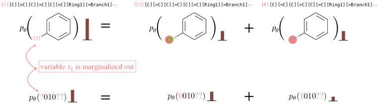
Figure 1: Marginalization models (MaMs) enable estimation of any marginal probability with a neural network $\theta$ that learns to “marginalize out” variables. The figure illustrates marginalization of a single variable on bit strings (representing molecules) with two alternatives (versus $K$ in general) for clarity. The bars represent probability masses.

To enhance scalability and flexibility in the generative modeling of discrete data, we propose a new family of generative models, marginalization models (MaMs), that directly model the marginal distribution $p(\mathbf{x}_{\mathcal{S}})$ for any subset of variables $\mathbf{x}_{\mathcal{S}}$ in $\mathbf{x}$. Direct access to marginals has two important advantages: 1) significantly speeding up inference for any marginal, and 2) enabling scalable training of any-order generative models under both MLE and EB settings.

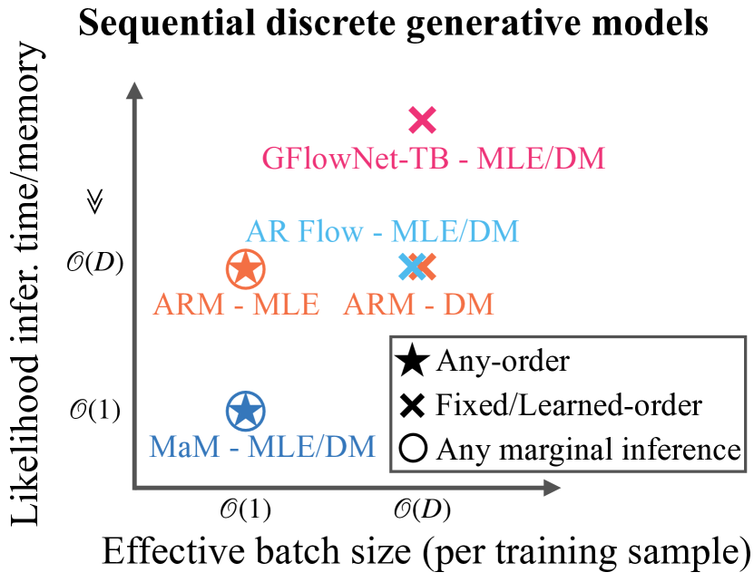
Figure 2: Scalability of sequential discrete generative models. The y-axis unit is # of NN forward passes required.

The unique structure of the model allows it to simultaneously represent the coupled collection of all marginal distributions of a given discrete joint probability mass function. For the model to be valid, it must be consistent with the sum rule of probability, a condition we refer to as “marginalization self-consistency” (see Figure 1); learning to enforce this with scalable training objectives is one of the key contributions of this work.

We show that MaMs can be trained under both maximum likelihood and energy-based training settings with scalable learning objectives. We demonstrate the effectiveness of MaMs in both settings on a variety of discrete data distributions, including binary images, text, physical systems, and molecules. We empirically show that MaMs achieve orders of magnitude speedup in marginal likelihood evaluation. For energy-based training, MaMs are able to scale training of any-order generative models to high-dimensional problems that previous methods fail to achieve.

2 Background

We first review two prevalent settings for training a generative model: maximum likelihood estimation and energy-based training. Then we introduce autoregressive models.

Maximum likelihood (MLE) Given a dataset $\mathcal{D}=\{\mathbf{x}^{(i)}\}_{i=1}^{N}$ drawn i.i.d. from a data distribution $p=p_{\text{data}}$, we aim to learn the distribution $p_{\theta}(\mathbf{x})$ via maximum likelihood estimation:

$$\max_{\theta}\;\mathbb{E}_{\mathbf{x}\sim p_{\text{data}}}\left[\log p_{\theta}(\mathbf{x})\right]\approx\max_{\theta}\;\frac{1}{N}\sum\nolimits_{i=1}^{N}\log p_{\theta}(\mathbf{x}^{(i)})$$ (1)

which is equivalent to minimizing the Kullback-Leibler divergence under the empirical distribution, i.e., minimizing $D_{\text{KL}}(p_{\text{data}}(\mathbf{x})||p_{\theta}(\mathbf{x}))$. This is the setting that is most commonly used in generation of images (e.g., diffusion models [59, 18, 60]) and language (e.g. GPT [49]) where we can easily draw observed data from the distribution.

Energy-based training (EB) In other cases, data from the distribution are not always available. Instead, we have access to an unnormalized probability distribution $f(\cdot)$ typically specified as ${f(\mathbf{x})=\exp(r(\mathbf{x})/\tau)}$ where $r(\mathbf{x})$ is an energy (or reward) function and $\tau>0$ is a temperature parameter. In this setting, the objective is to match $p_{\theta}(\mathbf{x})$ to $f(\mathbf{x})/Z$, where $Z$ is the normalization constant of $f$. This can be done by minimizing the KL divergence  [41, 72, 9],

$$\min_{\theta}\;D_{\text{KL}}\left(p_{\theta}(\mathbf{x})\|f(\mathbf{x})/{Z}\right)=\mathbb{E}_{\mathbf{x}\sim p_{\theta}(\mathbf{x})}\left[\log p_{\theta}\left(\mathbf{x}\right)-\log\left({f\left(\mathbf{x}\right)}/{Z}\right)\right],$$ (2)

The reward function $r(\mathbf{x})$ can be defined either by human preferences or by the physical system from first principles. For example, (a) In aligning large language models, $r(\mathbf{x})$ can represent human preferences [43, 42]; (b) In molecular/material design, it can specify the proximity of a sample’s measured or calculated properties to some functional desiderata [2]; and (c) In modeling the thermodynamic equilibrium ensemble of physical systems, it is the (negative) energy function of a given state [41, 72, 9].

The training objective in Equation 2 can be optimized with Monte Carlo estimate of the gradient using the REINFORCE algorithm [71]. The learned generative model $\theta$ allows us to efficiently generate samples approximately from the distribution of interest, which would otherwise be much more expensive via running MCMC with the energy function $f(\cdot)$.

Autoregressive models Autoregressive models (ARMs) [3, 30] model a complex high-dimensional distribution $p(\mathbf{x})$ by factorizing it into univariate conditionals using the chain rule:

$$\log p(\mathbf{x})=\sum\nolimits_{d=1}^{D}\log p\left(x_{d}\mid\mathbf{x}_{<d}\right),$$ (3)

where $\mathbf{x}_{<d}=\{x_{1},\ldots,x_{d-1}\}$. ARMs generate examples by sequentially drawing $x_{1}$ under $p(x_{1}),$ then $x_{2}$ under $p(x_{2}|x_{1}),$ and so on. The ARM approach has produced successful discrete-data neural models for natural language, proteins [58, 32, 36], and molecules [56, 15]. However, a key drawback of ARM is that evaluation of $p(\mathbf{x})$ or $p(\mathbf{x}_{s})$ requires $\mathcal{O}(D)$ neural network passes, making it costly for problems with high dimensions. This hinders ARM scalability for marginal inference during test time. Furthermore, in energy-based training, taking the gradient of Equation 2 that matches $p_{\theta}(\mathbf{x})$ to $f(\mathbf{x})/Z$ requires $\mathcal{O}(D)$ network passes per data sample. As a result, this significantly limits ARM’s training scalability under the EB setting for high-dimensional problems.

Any-order ARMs (AO-ARMs)  Uria et al. [66] propose to learn the conditionals of ARMs for arbitrary orderings that include all permutations of $\{1,\ldots,D\}$. Under the MLE setting, the model $\phi$ is trained by maximizing a lower-bound objective [66, 20] using an expectation under the uniform distribution of orderings. This objective allows scalable training of AO-ARMs, leveraging efficient parallel evaluation of multiple one-step conditionals for each token in one forward pass with architectures such as the U-Net [53] and Transformers [68]. However, modeling any-order conditionals alone presents training challenges in the EB setting. We discuss this issue in greater detail in Section 4.3.

3 Marginalization Models

We propose marginalization models (MaMs), a new type of generative model that enables scalable any-order generative modeling on high-dimensional problems as well as efficient marginal evaluation, for both maximum likelihood and energy-based training. The flexibility and scalability of marginalization models are enabled by the explicit modeling of the marginal distribution and enforcing marginalization self-consistency.

In this paper, we focus on generative modeling of discrete structures using vectors of discrete variables. The vector representation encompasses various real-world problems with discrete structures, including language sequence modeling, protein design, and molecules with string-based representations (e.g., SMILES [70] and SELFIES [29]). Moreover, vector representations are inherently applicable to any discrete problem, since it is feasible to encode any discrete object into a vector of discrete variables.

Definition Let $p(\mathbf{x})$ be a discrete probability distribution, where $\mathbf{x}=(x_{1},\ldots,x_{D})$ is a $D$-dimensional vector and each $x_{d}$ takes $K$ possible values, i.e. $x_{d}\in\mathcal{X}\triangleq\{1,\ldots,K\}$.

Marginalization Let $\mathbf{x}_{\mathcal{S}}$ be a subset of variables of $\mathbf{x}$ and $\mathbf{x}_{\mathcal{S}^{c}}$ be the complement set, i.e. $\mathbf{x}_{\mathcal{S}}\subseteq\{x_{1},\ldots,x_{D}\}$ and ${\mathbf{x}_{\mathcal{S}^{c}}=\{x_{1},\ldots,x_{D}\}\setminus\mathbf{x}_{\mathcal{S}}}$. The marginal of $\mathbf{x}_{\mathcal{S}}$ is obtained by summing over all values of $\mathbf{x}_{\mathcal{S}^{c}}$:

$$p(\mathbf{x}_{\mathcal{S}})=\sum\nolimits_{\mathbf{x}_{\mathcal{S}^{c}}}p(\mathbf{x}_{\mathcal{S}},\mathbf{x}_{\mathcal{S}^{c}})$$ (4)

We refer to (4) as the “marginalization self-consistency” that any valid distribution should follow. The goal of a marginalization model $\theta$ is to estimate the marginals $p(\mathbf{x}_{\mathcal{S}})$ for any subset of variables $\mathbf{x}_{\mathcal{S}}$ as closely as possible. To achieve this, we train a deep neural network $p_{\theta}$ that minimizes the distance of $p_{\theta}(\mathbf{x})$ and $p(\mathbf{x})$ on the full joint distribution while enforcing the marginalization self-consistency. In other words, MaM learns perform marginal inference over arbitrary subset of variables with a single forward pass.

Parameterization A marginalization model parameterized by a neural network $\theta$ takes in $\mathbf{x}_{\mathcal{S}}$ and outputs the marginal log probability $f_{\theta}(\mathbf{x}_{\mathcal{S}})=\log p_{\theta}(\mathbf{x}_{\mathcal{S}})$. Note that for different subsets $\mathcal{S}$ and $\mathcal{S}^{\prime}$, $\mathbf{x}_{\mathcal{S}}$ and $\mathbf{x}_{\mathcal{S}}^{\prime}$ lie in different vector spaces. To unify the vector space that is fed into the NN, we introduce an augmented vector space that additionally includes the “marginalized out” variables $\mathbf{x}_{\mathcal{S}^{c}}$ for an input $\mathbf{x}_{\mathcal{S}}$. By defining a special symbol “${\square}$” to denote the missing values of the “marginalized out” variables, the augmented vector representation is $D$-dimensional and is defined to be:

$$\mathbf{x}_{\mathcal{S}}^{\text{aug}}(i)=\begin{cases}x_{i},&\text{if }i\in\mathcal{S}\\ {\square},&\text{otherwise}\end{cases}$$

Now, the augmented vector representation $\mathbf{x}_{\mathcal{S}}^{\text{aug}}$ of all possible $\mathbf{x}_{\mathcal{S}}$’s have the same dimension $D$, and for any $i$-th dimension $\mathbf{x}_{\mathcal{S}}^{\text{aug}}(i)\in\mathcal{X}^{\text{aug}}\triangleq\{1,\cdots,K,{\square}\}$. For example, let $D=4$ and $\mathcal{X}=\{0,1\}$, for ${\mathbf{x}_{\mathcal{S}}=\{x_{1},x_{3}\}}$ with $x_{1}=0$ and $x_{3}=1$, ${\mathbf{x}_{\mathcal{S}}^{\text{aug}}=(0,{\square},1,{\square})}$, and $p(\mathbf{x}_{\mathcal{S}}^{\text{aug}})=\sum_{x_{2}}\sum_{x_{4}}p(0,x_{2},1,x_{4})$. From here onwards we will use $\mathbf{x}_{\mathcal{S}}^{\text{aug}}$ and $\mathbf{x}_{\mathcal{S}}$ interchangeably.

Sampling With the marginalization model, one can sample from the learned distribution by picking an arbitrary order and sampling one variable or multiple variables at a time. In this paper, we focus on the sampling procedure that generates one variable at a time. To get the conditionals at each step for generation, we can use the product rule of probability:

$$p_{\theta}(x_{\sigma(d)}|\mathbf{x}_{\sigma(<d)})=\frac{p_{\theta}(\mathbf{x}_{\sigma(\leq d)})}{p_{\theta}(\mathbf{x}_{\sigma(<d)})}\,,$$

However, the above sampling is not a valid conditional distribution if the following single-step marginalization consistency in (5) is not strictly enforced,

$$p_{\theta}(\mathbf{x}_{\sigma(<d)})=\sum\nolimits_{x_{\sigma(d)}}p_{\theta}(\mathbf{x}_{\sigma(\leq d)}),\quad\forall\sigma\in S_{D},\mathbf{x}\in\{1,\cdots,K\}^{D},d\in[1:D]\,,$$ (5)

since it might not sum up exactly to one. Hence we use following normalized conditional:

$$p_{\theta}(x_{\sigma(d)}|\mathbf{x}_{\sigma(<d)})=\frac{p_{\theta}([\mathbf{x}_{\sigma(<d)},x_{\sigma(d)}])}{\textstyle\sum\nolimits_{x_{\sigma(d)}}p_{\theta}([\mathbf{x}_{\sigma(<d)},x_{\sigma(d)}])}\,.$$ (6)

Scalable learning of marginalization self-consistency In training, we impose the marginalization self-consistency by minimizing the squared error of the constraints in (5) in log-space. Evaluation of each marginalization constraint in (5) requires $K$ NN forward passes, where $K$ is the number of discrete values $x_{d}$ can take. This makes mini-batch training challenging to scale when $K$ is large. To address this issue, we augment the marginalization models with learnable conditionals parameterized by another neural network $\phi$. The marginalization constraints in (5) can be further decomposed into $K$ parallel marginalization constraints.

$$p_{\theta}(\mathbf{x}_{\sigma(<d)})p_{\phi}(\mathbf{x}_{\sigma(d)}|\mathbf{x}_{\sigma(<d)})=p_{\theta}(\mathbf{x}_{\sigma(\leq d)}),\quad \forall\sigma\in S_{D},\mathbf{x}\in\{1,\cdots,K\}^{D},d\in[1:D].$$ (7)

By breaking the original marginalization self-consistency in Equation 4 into highly parallel marginalization self-consistency in Equation 7, we have arrived at $\mathcal{O}(K^{D}{\cdot}D{\cdot}D!)$ constraints. Although the number of constraints increases, it becomes highly scalable to train on the marginalization self-consistency via sampling the constraints. During training, we specify a distribution $q(\mathbf{x})$ for sampling the marginalization constraints. In practice, it can be set to the distribution of interest to perform marginal inference on, such as $p_{\text{data}}$ or the distribution of the generative model $p_{\theta,\phi}$. In empirical experiments, we found that training with objectives that decompose to highly parallel self-consistency errors is a key ingredient to learning marginals with scalability.

4 Training the Marginalization Models

4.1 Maximum Likelihood Estimation Training

In this setting, we train MaMs with the maximum likelihood objective while additionally enforcing the marginalization constraints in Equation 5:

$$\max_{\theta,\phi}\quad \mathbb{E}_{\mathbf{x}\sim p_{\text{data}}}\log p_{\theta}(\mathbf{x})$$ (8)

s.t. $$p_{\theta}(\mathbf{x}_{\sigma(<d)})p_{\phi}(\mathbf{x}_{\sigma(d)}|\mathbf{x}_{\sigma(<d)})=p_{\theta}(\mathbf{x}_{\sigma(\leq d)}),\;\forall\sigma\in S_{D},\mathbf{x}\in\{1,\cdots,K\}^{D},d\in[1:D].$$

Two-stage training A typical way to solve the above optimization problem is to convert the constraints into a penalty term and optimize the penalized objective, but we empirically found the learning to be slow and unstable. Instead, we identify an alternative two-stage optimization formulation that is theoretically equivalent to Equation 8, but leads to more efficient training:

Proposition 1.

Solving the optimization problem in (8) is equivalent to the following two-stage optimization procedure, under mild assumption about the neural networks used being universal approximators:

Stage 1: $$\max_{\phi}\;\mathbb{E}_{\mathbf{x}\sim p_{\text{data}}}\mathbb{E}_{\sigma\sim\mathcal{U}(S_{D})}\sum\nolimits_{d=1}^{D}\log p_{\phi}\left(x_{\sigma(d)}\mid\mathbf{x}_{\sigma(<d)}\right)$$

Stage 2: $$\min_{\theta}\;\mathbb{E}_{\mathbf{x}\sim q(\mathbf{x})}\mathbb{E}_{\sigma\sim\mathcal{U}(S_{D})}\mathbb{E}_{d\sim\mathcal{U}(1,\cdots,D)}\left(\log[p_{\theta}(\mathbf{x}_{\sigma(<d)})p_{\phi}(\mathbf{x}_{\sigma(d)}|\mathbf{x}_{\sigma(<d)})]-\log p_{\theta}(\mathbf{x}_{\sigma(\leq d)})\right)^{2}.$$

The first stage can be interpreted as fitting the conditionals in the same way as AO-ARMs [66, 20] and the second stage acts as distilling the marginals from conditionals. The intuition comes from the chain rule of probability: there is a one-to-one correspondence between optimal conditionals $\phi$ and marginals $\theta$, i.e. $\log p_{\theta}(\mathbf{x})=\sum\nolimits_{d=1}^{D}\log p_{\phi}\left(x_{\sigma(d)}|\mathbf{x}_{\sigma(<d)}\right)$ for any $\sigma$ and $\mathbf{x}$. By assuming neural networks are universal approximators, we can first optimize for the optimal conditionals, and then optimize for the corresponding optimal marginals. We provide proof details in Section A.1.

4.2 Energy-based Training

In this setting, we train MaMs using the energy-based training objective in Equation 2 with a penalty term to enforce the marginalization constraints in Equation 5:

$$\min_{\theta,\phi}D_{\text{KL}}\!\left(p_{\theta}\left(\mathbf{x}\right)\!\parallel\!p\!\left(\mathbf{x}\right)\right)+\lambda\,\mathbb{E}_{\mathbf{x}\sim q(\mathbf{x})}\mathbb{E}_{\sigma}\mathbb{E}_{d}\!\left(\log\!\left[p_{\theta}\!\left(\mathbf{x}_{\sigma(<d)}\right)p_{\phi}\!\!\left(\mathbf{x}_{\sigma(d)}|\mathbf{x}_{\sigma(<d)}\right)\right]-\log p_{\theta}\!\!\left(\mathbf{x}_{\sigma(\leq d}\right)\right)^{2}\!\!,$$

where $\sigma\sim\mathcal{U}(S_{D})$, $d\sim\mathcal{U}(1,\cdots,D)$ and $q(\mathbf{x})$ is the distribution of interest for evaluating marginals.

Scalable training We use REINFORCE [71] to estimate the gradient of the KL divergence term:

$$\nabla_{\theta}D_{\text{KL}}(p_{\theta}(\mathbf{x})||p(\mathbf{x})) =\mathbb{E}_{\mathbf{x}\sim p_{\theta}(\mathbf{x})}\left[\nabla_{\theta}\log p_{\theta}\left(\mathbf{x}\right)\left(\log p_{\theta}\left(\mathbf{x}\right)-\log f\left(\mathbf{x}\right)\right)\right]$$

$$\approx\nicefrac{{1}}{{N}}\sum\nolimits_{i=1}^{N}\nabla_{\theta}\log p_{\theta}(\mathbf{x}^{(i)})\left(\log p_{\theta}(\mathbf{x}^{(i)})-\log f(\mathbf{x}^{(i)})\right)$$ (9)

For the self-consistency penalty term, we sample data $\mathbf{x}$ from the specified data distribution of interest and sample the ordering $\sigma$, step $d$ from uniform distributions.

Efficient sampling with persistent MCMC We need cheap and effective samples from $p_{\theta}$ in order to perform REINFORCE, so a persistent set of Markov chains are maintained by randomly picking an ordering and taking block Gibbs sampling steps using the conditional distribution $p_{\phi}(\mathbf{x}_{\sigma(d)}|\mathbf{x}_{\sigma(<d)})$ (full algorithm in Section A.4), in similar fashion to persistent contrastive divergence [64]. The samples from the conditional network $p_{\phi}$ serve as approximate samples from the marginal network $p_{\theta}$ when they are close to each other. Otherwise, we can additionally use importance sampling to get an unbiased estimate.

4.3 Addressing limitations of ARMs

We discuss in more detail about how MaMs address some limitations of ARMs. The first one is general to both training settings, while the latter two are specific to energy-based training.

1) Slow marginal inference of likelihoods Due to sequential conditional modeling, evaluation of a marginal $p_{\phi}(\mathbf{x}_{o})$ with ARMs (or an arbitrary marginal with AO-ARMs) requires applying the NN $\phi$ up to $D$ times, which is inefficient in time and memory for high-dimensional data. In comparison, MaMs are able to estimate any arbitrary marginal with one NN forward pass.

2) Lack of support for any-order training In energy-based training, the objective in Equation 2 aims to minimize the distance between $\log p_{\phi}(\mathbf{x})$ and $\log p(x)$, where $\phi$ is the NN parameters of an ARM. However, unless the ARM is perfectly self-consistent over all orderings, it will not be the case that $\log p_{\phi}(\mathbf{x})=\mathbb{E}_{\sigma}\log p_{\phi}(\mathbf{x}|\sigma)$. Therefore, the expected $D_{\text{KL}}$ objective over the orderings $\sigma$ would not be equivalent to the original $D_{\text{KL}}$ objective, i.e., $\mathbb{E}_{\sigma}\,\mathbb{E}_{p_{\phi}(\cdot|\sigma)}D_{\text{KL}}(p_{\phi}(\cdot|\sigma)\|p)\neq\mathbb{E}_{p_{\phi}}D_{\text{KL}}(p_{\phi}\|p)$. As a result, ARMs cannot be trained with the expected $D_{\text{KL}}$ objective over all orderings simultaneously, but instead need to resort to a preset order and minimize the KL divergence between $\log p_{\phi}(\mathbf{x}|\sigma)$ and the target density $\log p(\mathbf{x})$.

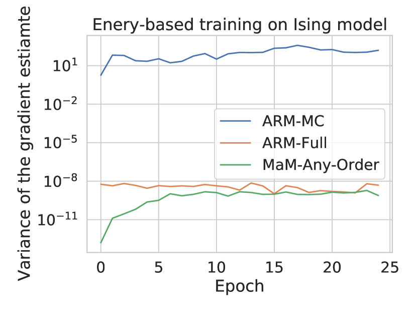
Figure 3: Approximating $\log p_{\phi}(\mathbf{x})$ with one-step conditional (ARM-MC) results in extremely high gradient variance during energy-based training.

The self-consistency constraints imposed by MaMs address this issue. MaMs are not limited to fixed ordering because marginals are order-agnostic and we can optimize over expectation of orderings for the marginalization self-consistency constraints.

3) Training not scalable on high-dimensional problems When minimizing the difference between $\log p_{\phi}(\mathbf{x}|\sigma)$ and the target $\log p(\mathbf{x})$, ARMs need to sum conditionals to evaluate $\log p_{\phi}(\mathbf{x}|\sigma)$. One might consider subsampling one-step conditionals $p_{\phi}(x_{\sigma(d)}|\mathbf{x}_{\sigma(<d})$ to estimate $p_{\phi}(\mathbf{x})$, but this leads to high variance of the REINFORCE gradient in Equation 9 due to the product of the score function and distance terms, which are both high variance (We validate this in experiments, see Figure 3). Consequently, training ARMs for energy-based training necessitates a sequence of $D$ conditional evaluations to compute the gradient of the objective function. This constraint leads to an effective batch size of $B\times D$ for batch of $B$ samples, significantly limiting the scalability of ARMs to high-dimensional problems. Furthermore, obtaining Monte Carlo samples from ARMs for the REINFORCE gradient estimator is slow when the dimension is high. Due to the fixed input ordering, this process requires $D$ sequential sampling steps, making more cost-effective sampling approaches like persistent MCMC infeasible. Marginalization models circumvent this challenge by directly estimating the log-likelihood with the marginal neural network. Additionally, the support for any-order training enables efficient sampling through the utilization of persistent MCMC methods.

5 Related Work

Autoregressive models Developments in deep learning have greatly advanced the performance of ARMs across different modalities, including images, audio, and text. Any-order (Order-agnostic) ARMs were first introduced in [66] by training with the any-order lower-bound objective for the maximum likelihood setting. Recent work, ARDM [20], demonstrates state-of-the-art performance for any-order discrete modeling of image/text/audio. Germain et al. [16] train an auto-encoder with masking that outputs the sequence of all one-step conditionals for a given ordering, but does not generate as well as methods [67, 73, 20] that predict one-step conditionals under the given masking. Douglas et al. [14] trains an AO-ARM as a proposal distribution and uses importance sampling to estimate arbitrary conditional probabilities in a DAG-structured Bayesian network, but with limited experiment validation on a synthetic dataset. Shih et al. [57] utilizes a modified training objective of ARMs for better marginal inference performance but loses any-order generation capability. In the energy-based training setting, ARMs are applied to science problems [9, 72], but suffer in scaling to when $D$ is large. MaMs and ARMs are compared in detail in Section 4.3.

Arbitrary conditional/marginal models For continuous data, VAEAC [25] and ACFlow [31] extends the idea of conditional variational encoder and normalizing flow to model arbitrary conditionals. ACE [62] improves the expressiveness of arbitrary conditional models through directly modeling the energy function, which reduces the constraints on parameterization but comes with the additional computation cost of to approximating the normalizing constant. Instead of using neural networks as function approximators, probabilistic circuits (PCs) [6, 45] offer tractable probabilistic models for both conditionals and marginals by building a computation graph with sum and product operations following specific structural constraints. Examples of PCs include Chow-Liu trees [7], arithmetic circuits [10], sum-product networks [47], etc. Peharz et al. [45] improved the scalability of PCs by combining arithmetic operations into a single monolithic einsum-operation and automatic differentiation. [33, 34] demonstrated the potential of PCs with distilling latent variables from trained deep generative models on continuous image data. However, expressiveness is still limited by the structural constraints. All methods mentioned above focus on MLE settings.

GFlowNets GFlowNets [2, 4] formulate the problem of generation as matching the probability flow at terminal states to the target normalized density. Compared to ARMs, GFlowNets allow flexible modeling of the generation process by assuming learnable generation paths through a directed acyclic graph (DAG). The advantages of learnable generation paths come with the trade-off of sacrificing the flexibility of any-order generation and exact likelihood evaluation. Under a fixed generation path, GFlowNets reduce to fixed-order ARMs [75]. In Section A.3, we further discuss the connections and differences between GFlowNets and AO-ARMs/MaMs. For discrete problems, Zhang et al. [76] train GFlowNets on the squared distance loss with the trajectory balance objective [38]. This is not scalable for large $D$ (for the same reason as ARMs in Section 4.3) and renders direct access to marginals unavailable. In the MLE setting, an energy function is additionally learned from data so that the model can be trained with energy-based training.

6 Experiments

We conduct experiments with marginalization models (MaM) on both MLE and EB settings for discrete problems including binary images, text, molecules and phyiscal systems. We consider the following baselines for comparison: Any-order ARM (AO-ARM) [20], ARM [30], GFlowNet [39, 76], Discrete Flow[65] and Probabilistic Circuit (PC)[45]. MaM, PC and (AO-)ARM support arbitrary marginal inference. Discrete flow allows exact likelihood evaluation while GFlowNet needs to approximate the likelihood with sum using importance samples. For evaluating AO-ARM’s marginal inference, we can either use an ensemble model by averaging over several random orderings (AO-ARM-E) or use a single random ordering (AO-ARM-S). In general, AO-ARM-E should always be better than AO-ARM-S but at a much higher cost. Neural network architecture and training hyperparameter details can be found in Appendix B.

6.1 Maximum Likelihood Estimation Training

Binary MNIST We report the negative test likelihood (bits/digit), marginal estimate quality and marginal inference time per minibatch (of size $16$) in Table (1). To keep GPU memory usage the same, we sequentially evaluate the likelihood for ARMs. Both MaM and AO-ARM use a U-Net architecture with 4 ResNet Blocks interleaved with attention layers (see Appendix B). GFlowNets fail to scale to large architectures as U-Net, hence we report GFlowNet results using an MLP from Zhang et al. [76]. For MaM, we use the conditional network to evaluate test likelihood (since this is also how MaM generates data). The marginal network is used for evaluating marginal inference. The quality of the marginal estimates will be compared to the best performing model.

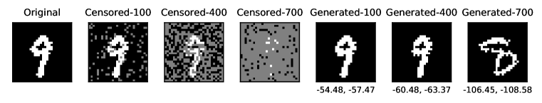
Figure 4: An example of the data generated (with $100/400/700$ pixels masked) for comparing the quality of likelihood estimate. Numbers below the images are LL estimates from MaM’s marginal network (left) and AO-ARM-E’s ensemble estimate (right).

Table 1: Performance Comparison on Binary-MNIST

Model	NLL (bpd) $\downarrow$	Spearman’s $\uparrow$	Pearson $\uparrow$	Marg. inf. time (s) $\downarrow$
AO-ARM-E-U-Net	0.148	1.0	1.0	661.98 $\pm$ 0.49
AO-ARM-S-U-Net	0.149	0.996	0.993	132.40 $\pm$ 0.03
GflowNet-MLP	0.189	–	–	–
PC-Image (EiNets)	0.187	0.716	0.752	0.015 $\pm$ 0.00
MaM-U-Net	0.149	0.992	0.993	0.018 $\pm$ 0.00

Table 2: Performance Comparison on Molecular Sets

Model	NLL (bpd) $\downarrow$	Spearman’s $\uparrow$	Pearson $\uparrow$	Marg. inf. time (s) $\downarrow$
AO-ARM-E-Transfomer	0.652	1.0	1.0	96.87$\pm$ 0.04
AO-ARM-S-Transfomer	0.655	0.996	0.994	19.32$\pm$ 0.01
MaM-Transfomer	0.655	0.998	0.995	0.006$\pm$0.00

Table 3: Performance Comparison on text8

Model	NLL (bpc) $\downarrow$	Spearman’s $\uparrow$	Pearson $\uparrow$	Marg. inf. time (s) $\downarrow$
Discrete Flow (8 flows)	1.23	–	–	–
AO-ARM-E-Transfomer	1.494	1.0	1.0	207.60 $\pm$ 0.33
AO-ARM-S-Transfomer	1.529	0.982	0.987	41.40 $\pm$ 0.01
MaM-Transfomer	1.529	0.937	0.945	0.005 $\pm$ 0.000

Table 4: Performance Comparison on Ising model ($10\times 10$)

Model	NLL (bpd) $\downarrow$	KL divergence $\downarrow$	Marg. inf. time (s) $\downarrow$
ARM-Forward-Order-MLP	0.79	-78.63	5.29$\pm$0.07e-01
ARM-MC-Forward-Order-MLP	24.84	-18.01	5.30$\pm$0.07e-01
GFlowNet-Learned-Order-MLP	0.78	-78.17	–
MaM-Any-Order-MLP	0.80	-77.77	3.75$\pm$0.08e-04

Table 5: Performance Comparison on Target Lipophilicity

Model	KL divergence $\downarrow$
Distribution	$\text{logP}=4$, $\tau=1.0$	$\text{logP}=-4$, $\tau=1.0$	$\text{logP}=4$, $\tau=0.1$	$\text{logP}=4$, $\tau=0.1$
ARM-FO-MLP	-174.25	-168.62	-167.83	-160.2
MaM-AO-MLP	-173.07	-166.43	-165.75	-157.59

In order to evaluate the quality of marginal likelihood estimates, we employ a controlled experiment where we randomly mask out portions of a test image and generate multiple samples with varying levels of masking (refer to Figure 4). This process allows us to obtain a set of distinct yet comparable samples, each associated with a different likelihood value. For each model, we evaluate the likelihood of the generated samples and compare that with AO-ARM-E’s estimate since it achieves the best likelihood on test data. We repeat this controlled experiment on a random set of test images. The mean Spearman’s and Pearson correlation are reported to measure the strength of correlation in marginal inference likelihoods between the given model and AO-ARM-E. MaM achieves close to $4$ order of magnitude speed-up in marginal inference while at comparable quality to that from AO-ARM-S. PCs are also very fast in marginal inference but there remains a gap in terms of quality. Generated samples and additional marginal inference on partial images are in Appendix B.

Molecular sets (MOSES) We test generative modeling of MaM on a benchmarking molecular dataset [46] refined from the ZINC database [61]. Same metrics are reported as Binary-MNIST. Likelihood quality is measured similarly but on random groups of test molecules instead of generated ones. The generated molecules from MaM and AO-ARM are comparable to standard state-of-the-art molecular generative models, such as CharRNN [56], JTN-VAE [26], and LatentGAN [48] (see Appendix B), with additional controllability and flexibility in any-order generation. MaM supports much faster marginal inference, which is useful for domain scientists to reason about likelihood of (sub)structures. Generated molecules and property histogram plots of are available in Appendix B.

Text8 Text8 [37] is a widely used character level natural language modeling dataset. The dataset comprises of 100M characters from Wikipedia, split into chunks of 250 character. We follow the same testing procedure as Binary-MNIST and report the same metrics. The test NLL of discrete flow is from [65], for which there are no open-source implementations to evaluate additional metrics.

6.2 Energy-based training

We compare with ARM that uses sum of conditionals to evaluate $\log p_{\phi}$ with fixed forward ordering and ARM-MC that uses a one-step conditional to estimate $\log p_{\phi}$. ARM can be regarded as the golden standard of learning autoregressive conditionals, since its gradient needs to be evaluated on the full generation trajectory, which is the most informative and costly. MaM uses marginal network to evaluate $\log p_{\theta}$ and subsamples a one-step marginalization constraint for each data point in the batch. The effective batch size for ARM and GFlowNet is $B\times\mathcal{O}(D)$ for batch of size $B$, and $B\times\mathcal{O}(1)$ for ARM-MC and MaM . MaM and ARM optimizes KL divergence using REINFORCE gradient estimator with baseline. GFlowNet is trained on per-sample gradient of squared distance [76].

Ising model Ising models [24] model interacting spins and are widely studied in mathematics and physics (see MacKay [35]). We study Ising model on a square lattice. The spins of the $D$ sites are represented a $D$-dimensional binary vector and its distribution is ${p^{*}(\mathbf{x})\propto f^{*}(\mathbf{x})=\exp\left(-\mathcal{E}_{J}(\mathbf{x})\right)}$ where ${\mathcal{E}_{\mathbf{J}}(\mathbf{x})\triangleq-\mathbf{x}^{\top}\mathbf{J}\mathbf{x}-\boldsymbol{\theta}^{\top}\mathbf{x}}$, with $\mathbf{J}$ the binary adjacency matrix. These models, although simplistic, bear analogies to the complex behavior of high-entropy alloys [9]. We compare MaM with ARM, ARM-MC, and GFlowNet on a ${10\!\times\!10}$ ($D\!=\!100$) and a larger ${30\!\times\!30}$ ($D\!=\!900$) Ising model where ARMs and GFlowNets fail to scale. $2000$ ground truth samples are generated following Grathwohl et al. [17] and we measure test negative log-likelihood on those samples. We also measure $D_{\text{KL}}(p_{\theta}(\mathbf{x})||p^{*})$ by sampling from the learned model and evaluating ${\sum_{i=1}^{M}(\log p_{\theta}(\mathbf{x}_{i})\!-\!\log f^{*}(\mathbf{x}_{i}))}$. Figure 5 contains KDE plots of $-\mathcal{E}_{\mathbf{J}}(\mathbf{x})$ for the generated samples. As described in Section 4.3, the ARM-MC gradient suffers from high variance and fails to converge. It also tends to collapse and converge to a single sample. MaM has significant speedup in marginal inference and is the only model that supports any-order generative modeling. The performance in terms of KL divergence and likelihood are only slightly worse than models with fixed/learned order, which is expected since any-order modeling is harder than fixed-order modeling, and MaM is solving a more complicated task of jointly learning conditionals and marginals. On a $30\times 30$ ($D=900$) Ising model, MaM achieves a bpd of $0.835$ on ground-truth samples while ARM and GFlowNet fails to scale. Distribution of generated samples is shown in Figure 5.

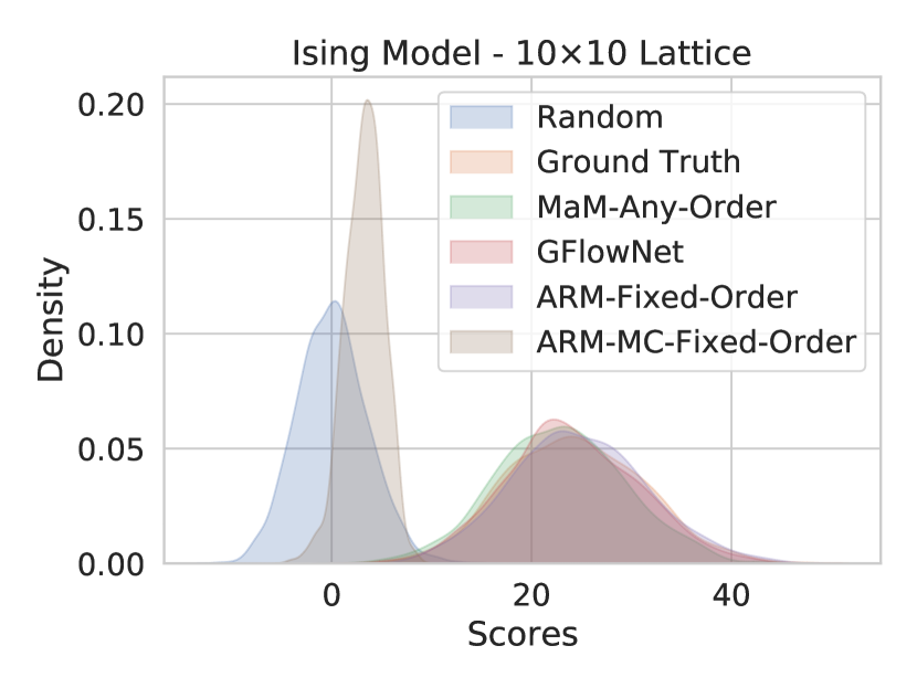
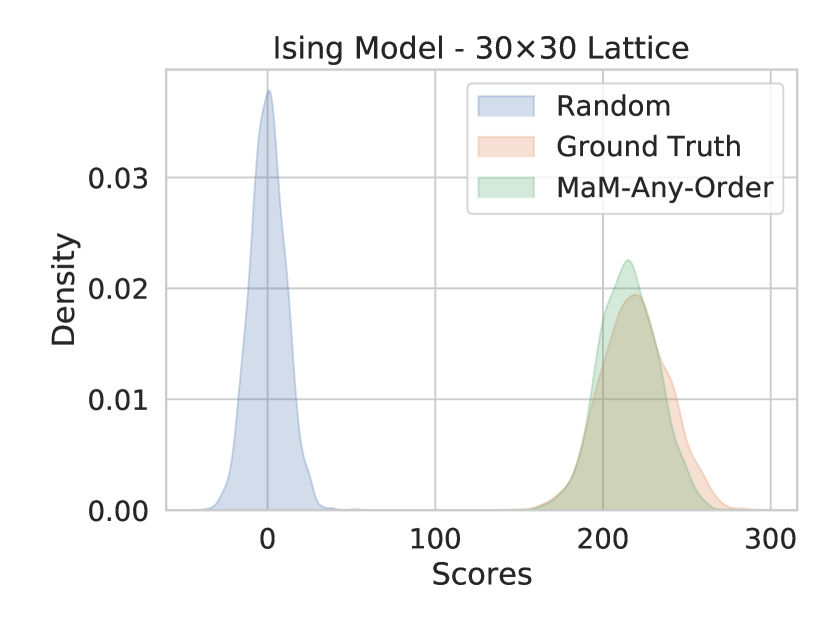
Figure 5: Ising model: $2000$ samples are generated for each method.

Molecular generation with target property In this task, we are interested in training generative models towards a specific target property of interest $g(x)$, such as lipophilicity (logP), synthetic accessibility (SA) etc. We define the distribution of molecules to follow ${p^{*}(x)\propto\exp(-(g(x)-g^{*})^{2}/\tau)}$, where $g^{*}$ is the target value of the property and $\tau$ is a temperature parameter. We train ARM and MaM for lipophilicity of target values $4.0$ and $-4.0$, both with $\tau=1.0$ and $\tau=0.1$. Both models are trained for $4000$ iterations with batch size $512$. Results are shown in Figure 6 and Table 5 (additional figures in Appendix B). Findings are consistent with the Ising model experiments. Again, MaM performs just marginally below ARM. However, only MaM supports any-order modeling and scales to high-dimensional problems. Figure 6 (right) shows molecular generation with MaM for $D=500$.

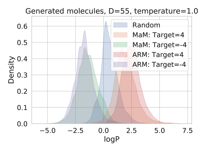
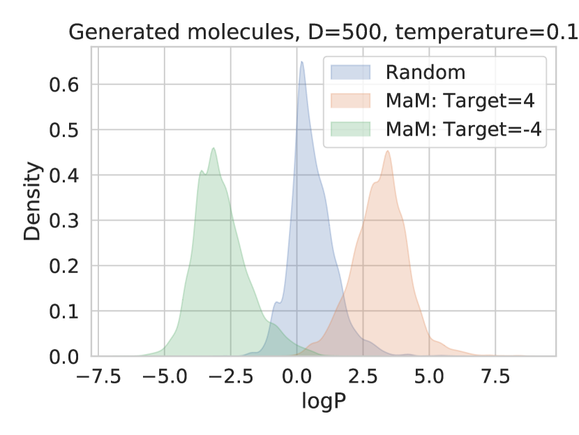
Figure 6: Target property matching: $2000$ samples are generated for each method.

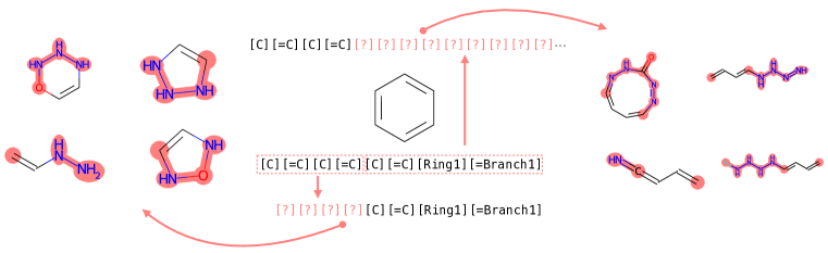
Figure 7: Conditionally generate towards low lipophilicity from a user-defined substructure in any given order. Left: Masking out the left 4 SELFIES characters. Right: Masking the right 4-20 SELFIES characters.

7 Conclusion

In conclusion, marginalization models are a novel family of generative models for high-dimensional discrete data that offer scalable and flexible generative modeling with tractable likelihoods. These models explicitly model all induced marginal distributions, allowing for fast evaluation of arbitrary marginal probabilities with a single forward pass of the neural network. MaMs also support scalable training objectives for any-order generative modeling, which previous methods struggle to achieve under the energy-based training setting. Potential future work includes designing new neural network architectures that automatically satisfy the marginalization self-consistency.

Acknowledgments

We thank members of the Princeton Laboratory for Intelligent Probabilistic Systems and anonymous reviewers for valuable discussions and feedback. We also want to thank Andrew Novick and Eric Toberer for valuable discussions on energy-based training in scientific applications. This work is supported in part by NSF grants IIS-2007278 and OAC-2118201.

Appendix A Additional Technical Details

A.1 Proof of Claim 1

Proof.

From the single-step marginalization self-consistency in (7), we have

$$\log p_{\theta}(\mathbf{x})=\sum\nolimits_{d=1}^{D}\log p_{\phi}\left(x_{\sigma(d)}|\mathbf{x}_{\sigma(<d)}\right),\;\forall\mathbf{x},\sigma.$$

Therefore we can rewrite the optimization in (8) as:

$$\max_{\phi}\quad \;\mathbb{E}_{\mathbf{x}\sim p_{\text{data}}}\mathbb{E}_{\sigma\sim\mathcal{U}(S_{D})}\sum\nolimits_{d=1}^{D}\log p_{\phi}\left(x_{\sigma(d)}\mid\mathbf{x}_{\sigma(<d)}\right)$$ (10)

s.t. $$p_{\theta}(\mathbf{x}_{\sigma(<d)})p_{\phi}(\mathbf{x}_{\sigma(d)}|\mathbf{x}_{\sigma(<d)})=p_{\theta}(\mathbf{x}_{\sigma(\leq d)}),\;\forall\sigma\in S_{D},\mathbf{x}\in\{1,\cdots,K\}^{D},d\in[1:D].$$

Let $p^{*}$ be the optimal probability distribution that maximizes the likelihood on training data, and from the chain rule we have:

$$p^{*}=\operatorname*{\arg\max}_{p}\mathbb{E}_{\mathbf{x}\sim p_{\text{data}}}\log p(\mathbf{x})=\mathbb{E}_{\mathbf{x}\sim p_{\text{data}}}\mathbb{E}_{\sigma\sim\mathcal{U}(S_{D})}\sum\nolimits_{d=1}^{D}\log p\left(x_{\sigma(d)}|\mathbf{x}_{\sigma(<d)}\right)$$

Then $p^{*}$ is also the optimal solution to (10) the marginalization constraints are automatically satisfied by $p^{*}$ since it is a valid distribution. From the universal approximation theorem [23, 22, 8], we can use separate neural networks to model $p_{\theta}$ (marginals) and $p_{\phi}$ (conditionals), and obtain optimal solution to (10) with $\theta^{*}$ and $\phi^{*}$ that approximates $p^{*}$ arbitrarily well.

Specifically, if $\theta^{*}$ and $\phi^{*}$ satisfy the following three conditions below, they are the optimal solution to (10):

$$p_{\phi^{*}}\left(x_{\sigma(d)}\mid\mathbf{x}_{\sigma(<d)}\right) =p^{*}\left(x_{\sigma(d)}\mid\mathbf{x}_{\sigma(<d)}\right),\quad\forall\;\mathbf{x},\sigma$$ (11)

$$p_{\theta^{*}}(\mathbf{x}_{s}) =p^{*}(\mathbf{x}_{s})Z_{\theta^{*}},\quad\forall\;\mathbf{x},s\subseteq\{1,\cdots,D\}$$ (12)

$$p_{\theta^{*}}(\mathbf{x}_{\sigma(<d)})p_{\phi^{*}}(\mathbf{x}_{\sigma(d)}|\mathbf{x}_{\sigma(<d)}) =p_{\theta^{*}}(\mathbf{x}_{\sigma(\leq d)}),\;\forall\sigma\in S_{D},\mathbf{x}\in\{1,\cdots,K\}^{D},d\in[1:D]$$ (13)

where $Z_{\theta^{*}}$ is the normalization constant of $p_{\theta^{*}}$ and is equal to $p_{\theta^{*}}([??\cdots?])$. It is easy to see from the definition of conditional probabilities that satisfying any two of the optimal conditions leads to the third one.

To obtain the optimal $\phi^{*}$, it suffices to solve the following optimization problem:

$$\textbf{Stage 1:}\quad\max_{\phi}\;\mathbb{E}_{\mathbf{x}\sim p_{\text{data}}}\mathbb{E}_{\sigma\sim\mathcal{U}(S_{D})}\sum\nolimits_{d=1}^{D}\log p_{\phi}\left(x_{\sigma(d)}\mid\mathbf{x}_{\sigma(<d)}\right)$$

because $p^{*}=\operatorname*{\arg\max}_{p}\mathbb{E}_{\mathbf{x}\sim p_{\text{data}}}\mathbb{E}_{\sigma\sim\mathcal{U}(S_{D})}\sum\nolimits_{d=1}^{D}\log p^{*}\left(x_{\sigma(d)}|\mathbf{x}_{\sigma(<d)}\right)$ due to chain rule. Solving Stage 1 is equivalent to finding $\phi^{*}$ that satisfies condition (11). Then we can obtain the optimal $\theta^{*}$ by solving for condition (13) given the optimal conditionals $\phi^{*}$:

$$\textbf{Stage 2:}\quad\min_{\theta}\;\mathbb{E}_{\mathbf{x}\sim q(\mathbf{x})}\mathbb{E}_{\sigma\sim\mathcal{U}(S_{D})}\mathbb{E}_{d\sim\mathcal{U}(1,\cdots,D)}\left(\log[p_{\theta}(\mathbf{x}_{\sigma(<d)})p_{\phi^{*}}(\mathbf{x}_{\sigma(d)}|\mathbf{x}_{\sigma(<d)})]-\log p_{\theta}(\mathbf{x}_{\sigma(\leq d)})\right)^{2}$$

∎

A.2 Expected Lower bound of Log-Likelihood

Here we present the expected lower bound objective used for training AO-ARMs under maximum likelihood setting, which was first proposed by Uria et al. [66]. Hoogeboom et al. [20] provided the expected lower bound perspective.

Given an ordering $\sigma$,

$$\log p(\mathbf{x}\mid\sigma)=\sum\nolimits_{d=1}^{D}\log p\left(x_{\sigma(d)}\mid\mathbf{x}_{\sigma(<d)}\right).$$ (14)

By taking the expectation over all orderings $\sigma$, we can derive a lower bound on the log-likelihood via Jensen’s inequality.

$$\log p_{\phi}(\mathbf{x})=\log\mathbb{E}_{\sigma}\,p_{\phi}(\mathbf{x}\mid\sigma) \overset{\text{Jensen's inequality}}{\geq}\mathbb{E}_{\sigma}\,\sum\nolimits_{d=1}^{D}\log p_{\phi}\left(x_{\sigma(d)}\mid\mathbf{x}_{\sigma(<d)}\right)$$

$$=\mathbb{E}_{\sigma\sim\mathcal{U}(S_{D})}\,D\,\mathbb{E}_{d\sim\mathcal{U}(1,\ldots,D)}\log p_{\phi}\left(x_{\sigma(d)}\mid\mathbf{x}_{\sigma(<d)}\right)$$

$$=D\,\mathbb{E}_{d}\,\mathbb{E}_{\sigma}\,\frac{1}{D-d+1}\sum\nolimits_{j\in\sigma(\geq d)}\log p_{\phi}\left(x_{j}\mid\mathbf{x}_{\sigma(<d)}\right),$$ (15)

where $\sigma\sim\mathcal{U}(S_{D})$, $d\sim\mathcal{U}(1,\ldots,D)$ and $\mathbf{x}_{\sigma(<d)}=\{x_{\sigma(1)},\ldots,x_{\sigma(d-1)}\}$. $\mathcal{U}(S)$ denotes the uniform distribution over a finite set $S$ and $\sigma(d)$ denotes the $d$-th element in the ordering.

A.3 Connections between MaMs and GFlowNets

In this section, we identify an interesting connection between generative marginalization models and GFlowNets. The two type of models are designed with different motivations. GFlowNets are motivated by learning a policy to generate according to an energy function and MaMs are motivated from any-order generation through learning to perform marginalization. However, under certain conditions, there exists an interesting connection between generative marginalization models and GFlowNets. In particular, the marginalization self-consistency condition derived from the definition of marginals in Equation 4 has an equivalence to the “detailed balance” constraint in GFlowNet under the following specific conditions.

Observation 1.

When the directed acyclic graph (DAG) used for generation in GFlowNet is specified by the following conditions, there is an equivalence between the marginalization self-consistency condition in Equation 7 for MaM and the detailed balance constraint proposed for GFlowNet [4]. In particular, the $p_{\theta}(x_{\sigma(d)}|\mathbf{x}_{\sigma(<d)})$ in MaM is equivalent to the forward policy $P_{F}(\mathbf{s}_{d+1}\mid\mathbf{s}_{d})$ in GFlowNet, and the marginals $p_{\theta}(x_{\sigma(d)})$ are equal to the flows $F(\mathbf{s}_{d})$ up to a normalizing constant.

• DAG Condition: The DAG used for generation in GFlowNet is defined by the given tree-like structure: a sequence $\mathbf{x}$ is generated by incrementally adding one variable at each step, following a uniformly random ordering $\sigma$ i.e. $\sigma\sim\mathcal{U}(S_{D})$. At step $d$, the state along the generation trajectory is defined to be $\mathbf{s}_{d}=\mathbf{x}_{\sigma(\leq d)}$.

• Backward Policy Condition: At step $D-d$, the backward policy under the DAG is fixed by removing (un-assigning) the value of the $d+1$-th element under ordering $\sigma$ , i.e. $P_{B}(\mathbf{s}_{d}\mid\mathbf{s}_{d+1};\sigma)=\mathbbm{1}_{\{\mathbf{s}_{d}=\mathbf{x}_{\sigma(\leq d)}\}}$. Or equivalently, the backward policy removes (un-assigns) one of the existing variables at random, i.e. $P_{B}(\mathbf{s}_{d}\mid\mathbf{s}_{d+1})=\nicefrac{{1}}{{d+1}}\mathbbm{1}_{\{\mathbf{s}_{d}\subset\mathbf{s}_{d+1}\}}$.

Intuitively, this is straight forward to understand, since GFlowNet generates a discrete object autoregressively. The model was proposed to enhance the flexibility of generative modeling by allowing for a learned ordering, as compared with auto-regressive models (see [76] Sec. 5 for a discussion). When the generation ordering is fixed, it is reduced to autoregressive models with fixed ordering, which is discussed in [75]. 1 presented above for any-order ARMs can be seen as a extended result of the connection between GFlowNets and fixed-order ARMs.

We have seen the interesting connection of GFlowNets with ARMs (and MaMs). Next, we discuss the differences between GFlowNets and MaMs.

Remark 1.

The detailed balance constraint was proposed only as a theoretical result in Bengio et al. [4]. In actual experiments, GFlowNets are trained using either flow matching [2] or trajectory balance [38, 76].

Zhang et al. [76] is the most relevant GFlowNet work that targets the discrete problem setting. Training is done via minimizing the squared distance loss with trajectory balance objective. For the MLE training, it proposes to additionally learn an energy function from data so that the trajectory balance objetive can still be applied. In particular, MaM is different from GFlowNet in Zhang et al. [76] in three main aspects.

• First of all, MaMs target any-order generation and direct access to marginals, where as GFlowNets aim for flexibility in learning generation paths and does not offer exact likelihood or direct access to marginals under learnable generation paths. When the generation path is fixed to follow a ordering or random ordering, they are reduced to ARMs or any-order ARMs, which allow for exact likelihood. However, training with the trajectory balance objective does not offer direct access to marginals (just like how ARMs do not offer direct access to marginals but only conditionals).

• Second, training under MLE setting is signiticantly different: GFlowNets learn an additional learned energy function to reduce MLE training back to energy-based training, while MaMs directly maximizes the expected lower bound on the log-likelihood under the marginalization self-consistent constraint.

• Lastly, the training objective is different under energy-based training. GFlowNets are trained on squared distance under the expectation to be specified to be either on-policy, off-policy, or a mixture of both. MaMs are trained on KL divergence where the expectation is defined to be on-policy. It is possible though to train MaMs with squared distance and recently Malkin et al. [39] have shown the equivalence of the gradient of KL divergence and the on-policy expectation of the per-sample gradient of squared distance (which is the gradient actually used for training GFlowNets).

A.4 Algorithms

We present the algorithms for training MaM for maximum likelihood and energy-based training settings in Algorithm 1 and Algorithm 2.

Algorithm 1 MLE training of MaMs

Input: Data $\mathcal{D}_{\text{train}}$, $q(\mathbf{x})$, network $\theta$ and $\phi$

Stage 1: Train $\phi$ with Equation 15 used in AO-ARM

for minibatch $\mathbf{x}\sim\mathcal{D}_{\text{train}}$ do

     Sample $\sigma\sim\mathcal{U}(S_{D})$, $d\sim\mathcal{U}(1,\cdots,D)$

     $\mathcal{L}\leftarrow\frac{D}{D-d+1}\sum\nolimits_{j\in\sigma(\geq d)}\log p_{\phi}\left(x_{j}|\mathbf{x}_{\sigma(<d)}\right)$

     Update $\phi$ with gradient of $\mathcal{L}$

end for

Stage 2: Train $\theta$ to distill the marginals from optimized conditionals $\phi$

for minibatch $\mathbf{x}\sim q(\mathbf{x})$ do

     Sample $\sigma\sim\mathcal{U}(S_{D})$, $d\sim\mathcal{U}(1,\cdots,D)$

     $\mathcal{L}\leftarrow$ squared error of the inconsistencies in Equation 7

     Update $\theta$ with gradient of $\mathcal{L}$

end for

Algorithm 2 Energy-based training of MaMs

Input: $q(\mathbf{x})$, network $\theta$ and $\phi$, Gibbs sampling block size $M$

Joint training of $\phi$ and $\theta$:

for $j$ in $\{1,\cdots,N\}$ do

     Sample $\sigma\sim\mathcal{U}(S_{D})$

     Update $\mathbf{x}\sim p_{\phi}(\mathbf{x}_{\sigma(\leq M)}|\mathbf{x}_{\sigma(>M)})$

$\triangleright$ Persistent block Gibbs sampling

     Sample $\tilde{\mathbf{x}}\sim q(\mathbf{x})$

     Sample $\tilde{d}\sim\mathcal{U}(1,\cdots,D)$, $\tilde{\sigma}\sim\mathcal{U}(S_{D})$

     $\mathcal{L}_{\text{penalty}}\leftarrow$ squared error of Equation 7, for $\tilde{d}$ and $\tilde{\sigma}$ with $\tilde{\mathbf{x}}$

     $\nabla_{\theta,\phi}D_{\text{KL}}\leftarrow$ REINFORCE est. with $\mathbf{x}$

     $\nabla_{\theta,\phi}\leftarrow\nabla_{\theta,\phi}D_{\text{KL}}+\lambda\nabla_{\theta,\phi}\mathcal{L}_{\text{penalty}}$

     Update $\theta$ and $\phi$ with gradient

end for

A.5 Additional literature on discrete generative models

Discrete diffusion models Discrete diffusion models learn to denoise from a latent base distribution into the data distribution. Sohl-Dickstein et al. [59] first proposed diffusion for binary data and was extended in Hoogeboom et al. [21] for categorical data and both works adds uniform noise in the diffusion process. A wider range of transition distributions was proposed in Austin et al. [1] and insert-and-delete diffusion processes have been explored in Johnson et al. [27]. Hoogeboom et al. [20] explored the connection between ARMs and diffusion models with absorbing diffusion and showed that OA-ARDMs are equivalent to absorbing diffusion models in infinite time limit, but achieves better performance with a smaller number of steps.

Discrete normalizing flow Normalizing flows transform a latent base distribution into the data distribution by applying a sequence of invertible transformations [52, 63, 12, 59, 51, 13, 28, 44]. They have been extended to discrete data [65, 19] with carefully designed discrete variable transformations. Their performance is competitive on character-level text modeling, but they do not allow any-order modeling and could be limited to discrete data with small number of categories due to the use of a straight-through gradient estimators.

Appendix B Additional Experiments Details

B.1 Dataset details

Binary MNIST Binary MNIST is a dataset introduced in [54] that stochastically set each pixel to $1$ or $0$ in proportion to its pixel intensity. We use the training and test split of [54] provided in https://github.com/yburda/iwae/tree/master [5].

To evaluate the quality of the likelihood estimates, we employ a controlled experiment where we randomly mask out portions ($100$, $400$, and $700$ pixels) of a test image and generate multiple samples with varying levels of masking (refer to Figure 4). We repeat this for $160$ (randomly subsampled) test images and created a dataset of $640$ sets of comparable images. To further test the quality of the marginal likelihood estimates on partially observed images, we curate a dataset of $160$ sets of partial test images ($7\sim 9$ images in each set) by randomly subsampling from the test set and masking the upper half of the images. To make sure the partial images are comparable but different in their log-likelihood, in each set, we remove samples that have a log-likelihood close to another sample within the threshold of $5.0$.

Molecular Sets The molecules in MOSES are represented either in SMILES [70] or SELFIES [29] strings. We construct a vocabulary (including a stop token) from all molecules and use discrete valued strings to represent molecules. It is worth noting that MaM can also be applied for modeling molecules at a coarse-grained level with predefined blocks, which we leave for future work.

The test set used for evaluating likelihood estimate quality is constructed in a similar manner to Binary MNIST, by drawing sets of random samples from the test dataset.

text8 In this dataset, we use a vocabulary of size $27$ to represent the letter alphabet with an extra value to represent spaces.

The test set of datasets used for evaluating likelihood estimate quality is constructed in a similar manner to Binary MNIST, each set is generated by randomly masking out portions of a test text sequence (by $50$, $100$, $150$, $200$ tokens) and generating samples.

Ising model The Ising model is defined on a 2D cyclic lattice. The $\mathbf{J}$ matrix is defined to be $\sigma\mathbf{A}_{N}$, where $\sigma$ is a scalar and $\mathbf{A}_{N}$ is the adjacency matrix of a $N\times N$ grid. Positive $\sigma$ encourages neighboring sites to have the same spins and negative $\sigma$ encourages them to have opposite spins. The bias term $\boldsymbol{\theta}$ places a bias towards positive or negative spins. In our experiments, we set $\sigma$ to $0.1$ and $\boldsymbol{\theta}$ to $\mathbf{1}$ scaled by $0.2$. Since we only have access to the unnormalized probability, we generate $2000$ samples following [17] using Gibbs sampling with $1,000,000$ steps for $10\times 10$ and $30\times 30$ lattice sizes. Those data serve as ground-truth samples from the Ising model for evaluating the test log-likelihood.

Molecular generation with target property During training, we need to optimize on the loss objective on samples generated from the neural network model. However, if the model generates SMILES strings, not all strings correspond to a valid molecule, which makes training at the start challenging when most generated SMILES strings are invalid molecules. Therefore, we use SELFIES string representation as it is a $100\%$ robust in that every SELFIES string corresponds to a valid molecule and every molecule can be represented by SELFIES.

B.2 Training details

Binary MNIST

• $0$, $1$ and “?” are represented by a scalar value (“?” takes the value $0$) and additionally a mask indicating if it is a “?”.

• U-Net with 4 ResNet Blocks interleaved with attention layers for both AO-ARM and MaM. MaM uses two separate neural networks for learning marginals $\phi$ and conditionals $\theta$. Input resolution is $28\times 28$ with $256$ channels used.

• The mask is concatenated to the input. $3/4$ of the channels are used to encode input. The remaining $1/4$ channels encode the mask cardinality (see [20] for details).

• MaM first learns the conditionals $\phi$ and then learns the marginals $\theta$ by finetuning on the downsampling blocks and an additional MLP with $2$ hidden layers of dimension $4096$. We observe it is necessary to finetune not only on the additional MLP but also on the downsampling blocks to get a good estimate of the marginal probability, which shows marginal network and conditional network rely on different features to make the final prediction.

• Batch size is $128$, Adam is used with learning rate $0.0001$. Gradient clipping is set to $100$. Both AO-ARM and MaM conditionals are trained for $600$ epochs. The MaM marginals are finetuned from the trained conditionals for $100$ epochs.

MOSES and text8

• Transformer with $12$ layers, $768$ dimensions, $12$ heads, $3072$ MLP hidden layer dimensions for both AO-ARM and MaM. Two separate networks are used for MaM.

• SMILES or SELFIES string representation and “?” are first converted into one-hot encodings as input to the Transformer.

• MaM first learns the conditionals $\phi$ and then learns the marginals $\theta$ by finetuning on the MLP of the Transformer.

• Batch size is $512$ for MOSES and $256$ for text8.

• AdamW is used with learning rate $0.0005$, betas $0.9/0.99$, weight decay $0.001$. Gradient clipping is set to $0.25$. Both AO-ARM and MaM conditionals are trained for $1000$ epochs for text8 and $200$ epochs for MOSES. The MaM marginals are finetuned from the trained conditionals for $200$ epochs.

Ising model and molecule generation with target property

• Ising model input are of $\{0,1,?\}$ values and are one-encoded as input to the neural network. The same is done for molecule SELFIES strings.

• MLP with residual layers, $3$ hidden layers, feature dimension is $2048$ for Ising model. $6$ hidden layers, feature dimension $4096$ for molecule target generation.

• Adam is used with learning rate of $0.0001$. Batch size is $512$ and $4096$ for molecule target generation. ARM, GFlowNet and MaM are trained with $19,800$ steps for the Ising model. ARM and MaM are trained with $3,000$ steps for molecule target generation.

• Separate networks are used for conditionals and marginals of MaM. They are trained jointly with penalty parameter $\lambda$ set to $4$.

Compute

• All models are trained on a single NVIDIA A100. The evaluation time is tested on an NVIDIA GTX 1080Ti.

B.3 Additional results on Binary MNIST

Likelihood estimate on partial Binary MNIST images

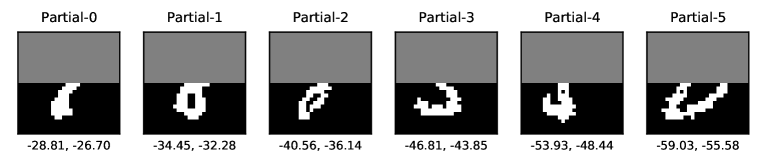
Figure 8: An example set of partial images for evaluating marginal likelihood estimate quality. The numbers in the captions show the log-likelihood calculated using learned marginals (left) v.s. learned conditionals (right)

Figure 8 illustrates an example set of partial images that we evaluate and compare likelihood estimate from MaM against ARM. Table 6 contains the comparison of the marginal likelihood estimate quality and inference time.

Table 6: Performance Comparison on Binary-MNIST partial images

Model	Spearman’s $\uparrow$	Pearson $\uparrow$	Marg. inf. time (s) $\downarrow$
AO-ARM-E-U-Net	1.0	1.0	248.96 $\pm$ 0.14
AO-ARM-S-U-Net	1.0	0.997	49.75 $\pm$ 0.03
MaM-U-Net	0.998	0.995	0.02 $\pm$ 0.00

Generated image samples

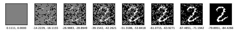
Figure 9: An example of the trajectory every $112$ step when generating an MNIST digit following a random order. The future pixels are generated by conditioning on the existent filled-in pixels. The numbers in the captions show the log-likelihood calculated using learned marginals (left) v.s. learned conditionals (right)

Figure 9 shows how a digit is generated pixel-by-pixel following a random order. We show generated samples from MaM using the learned conditionals $\phi$ in Figure 10.

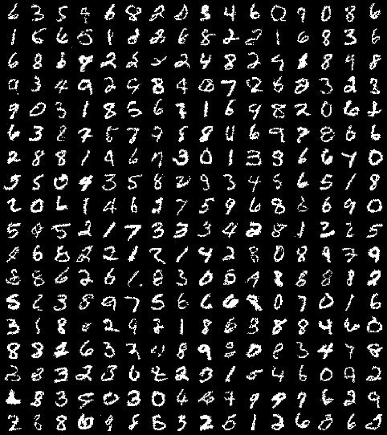
Figure 10: Generated samples: Binary MNIST

B.4 Additional results on MOSES

Table 7: Performance Comparison on MOSES

Model	Valid$\uparrow$	Unique 10k$\uparrow$	Frag Test$\downarrow$	Scaf TestSF$\uparrow$	Int Div1$\uparrow$	Int Div2$\uparrow$	Filters$\uparrow$	Novelty$\uparrow$
Train	1.0	1.0	1.0	0.9907	0.8567	0.8508	1.0	1.0
HMM	0.076	0.5671	0.5754	0.049	0.8466	0.8104	0.9024	0.9994
NGram	0.2376	0.9217	0.9846	0.0977	0.8738	0.8644	0.9582	0.9694
CharRNN	0.9748	0.9994	0.9998	0.1101	0.8562	0.8503	0.9943	0.8419
JTN-VAE	1.0	0.9996	0.9965	0.1009	0.8551	0.8493	0.976	0.9143
MaM-SMILES	0.7192	0.9999	0.9978	0.1264	0.8557	0.8499	0.9763	0.9485
MaM-SELFIES	1.0	0.9999	0.997	0.0943	0.8684	0.8625	0.894	0.9155

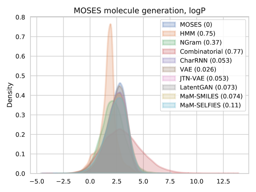
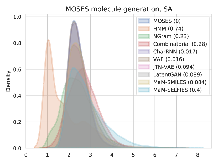
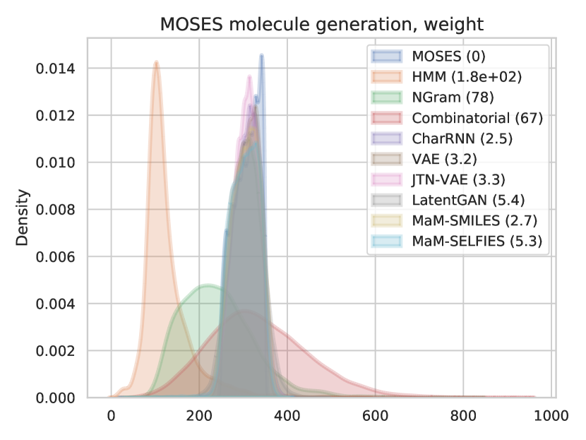
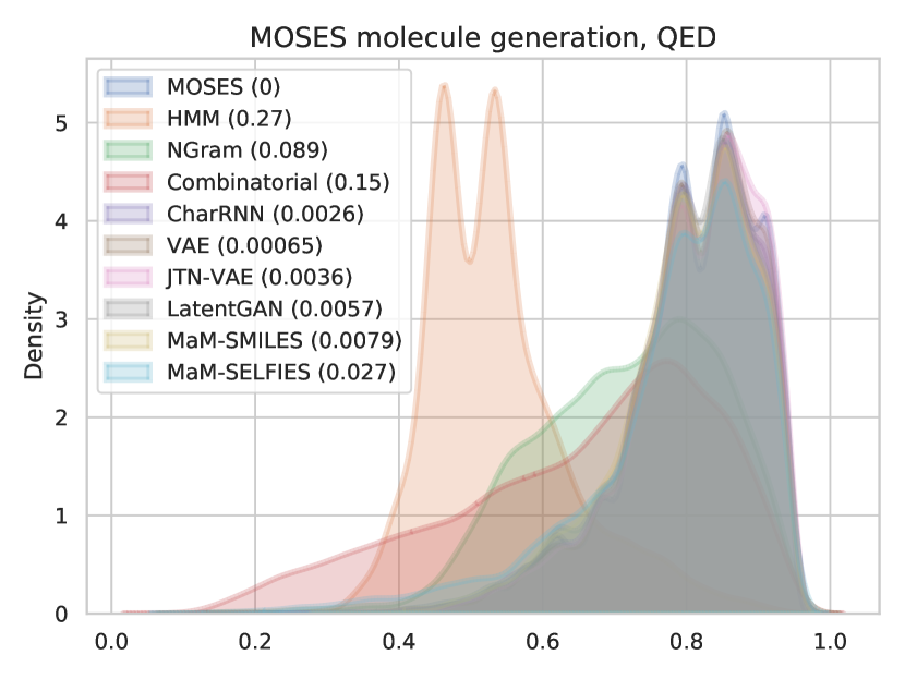
Figure 11: KDE plots of lipophilicity (logP), Synthetic Accessibility (SA), Quantitative Estimation of Drug-likeness (QED), and molecular weight for generated molecules. $30,000$ molecules are generated for each method.

Comparing MaM with SOTA on MOSES molecule generation

We compare the quality of molecules generated by MaM with standard baselines and state-of-the-art methods in Table 7 and Figure 11. Details of the baseline methods are provided in [46]. MaM-SMILES/SELFIES represents MaM trained on SMILES/SELFIES string representations of molecules. MaM performs either better or comparable to SOTA molecule generative modeling methods. The major advantage of MaM and AO-ARM is that their order-agnostic modeling enables generation in any desired order of the SMILES/SELFIES string (or molecule sub-blocks).

Generated molecular samples

Figure 12 and 13 plot the generated molecules from MaM-SMILES and MaM-SELFIES.

[width=1]svg-inkscape/samples_moese_smiles_svg-tex.pdf_tex

Figure 12: Generated samples from MaM-SMILES: MOSES

[width=1]svg-inkscape/samples_moses_selfies_svg-tex.pdf_tex

Figure 13: Generated samples from MaM-SELFIES: MOSES

B.5 Additional results on text8

Samples used for evaluating likelihood estimate quality

We show an example of a set of generated samples from masking different portions of the same text, which is then used for evaluating and comparing the likelihood estimate quality. Their log-likelihood calculated using the conditionals with the AO-ARM are in decreasing order. We use MaM marginal network to evaluate the log-likelihood and compare its quality with that of the AO-ARM conditionals.

B.6 Additional experiments on Ising model

Generated samples

We compare ground truth samples and MaM samples in Figure 14 and 15.

Figure 14: Samples: $10\times 10$ Ising model. Ground truth (left) v.s. MaM (right).

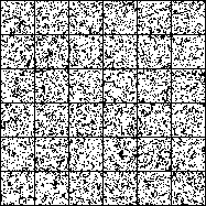
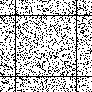
Figure 15: Samples: $30\times 30$ Ising model. Ground truth (left) v.s. MaM (right).

B.7 Additional experiments on molecule target generation

Target property energy-based training on lipophilicity (logP)

Figure 16 and 17 show the logP of generated samples of length $D=55$ towards target values $4.0$ and $-4.0$ under distribution temperature $\tau=1.0$ and $\tau=0.1$. For $\tau=1.0$, the peak of the probability density (mass) appears around $2.0$ (or $-2.0$) because there are more valid molecules in total with that logP than molecules with $4.0$ (or $-4.0$), although a single molecule with $4.0$ (or $-4.0$) has a higher probability than $2.0$ (or $-2.0$). When the temperature is set to much lower ($\tau=0.1$), the peaks concentrate around $4.0$ (or $-4.0$) because the probability of logP value being away from $4.0$ (or $-4.0$) quickly diminishes to zero. We additionally show results on molecules of length $D=500$. In this case, logP values are shifted towards the target but their peaks are closer to $0$ than when $D=55$, possibly due to the enlarged molecule space containing more molecules with logP around 0. Also, this is validated by the result when $\tau=0.1$ for $D=500$, the larger design space allows for more molecules with logP values that are close to, but not precisely, the target value.

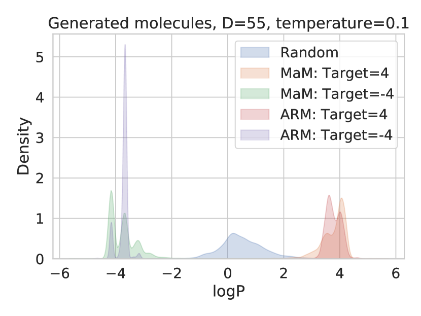
Figure 16: Target property matching with different temperatures. $2000$ samples are generated for each method.

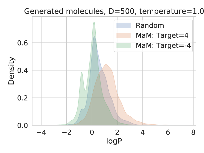
Figure 17: Target property matching with different temperatures. $2000$ samples are generated for each method.

Conditionally generated samples

More samples from conditionally generating towards low lipophilicity ($\text{target}=-4.0$, $\tau=1.0$) from user-defined substructures of Benzene. We are able to generate from any partial substructures with any-order generative modeling of MaM. Figure 18 shows conditional generation from masking out the left $4$ SELFIES characters. Figure 19 shows conditional generation from masking the right $4\sim 20$ characters.

[width=1]svg-inkscape/cond_gen_0_4_svg-tex.pdf_tex

Figure 18: Generated samples from masking out the left 4 SELFIES characters of a Benzene.

[width=1]svg-inkscape/cond_gen_4_20_svg-tex.pdf_tex

Figure 19: Generated samples from masking out the right 4-20 SELFIES characters of a Benzene.

Appendix C Limitations and Broader Impacts

The marginalization self-consistency in MaM is only softly enforced by minimizing the squared error on subsampled marginalization constraints. Therefore the marginal likelihood estimate is not guaranteed to be always perfectly valid. In particular, as a deep learning model, it has the risk of overfitting and low robustness on unseen data distribution. In practice, it means one should not blindly apply it to data that is very different from the training data and expect the marginal likelihood estimate can be trusted.

MaM enables training of a new type of generative model. Access to fast marginal likelihood is helpful for many downstream tasks such as outlier detection, protein/molecule design or screening. By allowing the training of order-agnostic discrete generative models scalable for energy-based training, it enhances the flexibility and controllability of generation towards a target distribution. This also poses the potential risk of deliberate misuse, leading to the generation of content/designs/materials that could cause harm to individuals.

References

- Austin et al. [2021] Jacob Austin, Daniel D Johnson, Jonathan Ho, Daniel Tarlow, and Rianne van den Berg. Structured denoising diffusion models in discrete state-spaces. Advances in Neural Information Processing Systems, 34:17981–17993, 2021.
- Bengio et al. [2021] Emmanuel Bengio, Moksh Jain, Maksym Korablyov, Doina Precup, and Yoshua Bengio. Flow network based generative models for non-iterative diverse candidate generation. Advances in Neural Information Processing Systems, 34:27381–27394, 2021.
- Bengio & Bengio [2000] Samy Bengio and Yoshua Bengio. Taking on the curse of dimensionality in joint distributions using neural networks. IEEE Transactions on Neural Networks, 11(3):550–557, 2000.
- Bengio et al. [2023] Yoshua Bengio, Salem Lahlou, Tristan Deleu, Edward J. Hu, Mo Tiwari, and Emmanuel Bengio. Gflownet foundations. Journal of Machine Learning Research, 24(210):1–55, 2023.
- Burda et al. [2015] Yuri Burda, Roger Grosse, and Ruslan Salakhutdinov. Importance weighted autoencoders. arXiv preprint arXiv:1509.00519, 2015.
- Choi et al. [2020] Y Choi, Antonio Vergari, and Guy Van den Broeck. Probabilistic circuits: A unifying framework for tractable probabilistic models. UCLA. URL: http://starai. cs. ucla. edu/papers/ProbCirc20. pdf, 2020.
- Chow & Liu [1968] CKCN Chow and Cong Liu. Approximating discrete probability distributions with dependence trees. IEEE transactions on Information Theory, 14(3):462–467, 1968.
- Cybenko [1989] George Cybenko. Approximation by superpositions of a sigmoidal function. Mathematics of control, signals and systems, 2(4):303–314, 1989.
- Damewood et al. [2022] James Damewood, Daniel Schwalbe-Koda, and Rafael Gómez-Bombarelli. Sampling lattices in semi-grand canonical ensemble with autoregressive machine learning. npj Computational Materials, 8(1):61, 2022.
- Darwiche [2003] Adnan Darwiche. A differential approach to inference in Bayesian networks. Journal of the ACM (JACM), 50(3):280–305, 2003.
- Devlin et al. [2018] Jacob Devlin, Ming-Wei Chang, Kenton Lee, and Kristina Toutanova. Bert: Pre-training of deep bidirectional transformers for language understanding. arXiv preprint arXiv:1810.04805, 2018.
- Dinh et al. [2014] Laurent Dinh, David Krueger, and Yoshua Bengio. NICE: Non-linear independent components estimation. arXiv preprint arXiv:1410.8516, 2014.
- Dinh et al. [2016] Laurent Dinh, Jascha Sohl-Dickstein, and Samy Bengio. Density estimation using real NVP. arXiv preprint arXiv:1605.08803, 2016.
- Douglas et al. [2017] Laura Douglas, Iliyan Zarov, Konstantinos Gourgoulias, Chris Lucas, Chris Hart, Adam Baker, Maneesh Sahani, Yura Perov, and Saurabh Johri. A universal marginalizer for amortized inference in generative models. Advances in Approximate Bayesian Inference, NIPS 2017 Workshop, 2017.
- Flam-Shepherd et al. [2022] Daniel Flam-Shepherd, Kevin Zhu, and Alán Aspuru-Guzik. Language models can learn complex molecular distributions. Nature Communications, 13(1):3293, 2022.
- Germain et al. [2015] Mathieu Germain, Karol Gregor, Iain Murray, and Hugo Larochelle. Made: Masked autoencoder for distribution estimation. In International conference on machine learning, pp. 881–889. PMLR, 2015.
- Grathwohl et al. [2021] Will Grathwohl, Kevin Swersky, Milad Hashemi, David Duvenaud, and Chris Maddison. Oops I took a gradient: Scalable sampling for discrete distributions. In International Conference on Machine Learning, pp. 3831–3841. PMLR, 2021.
- Ho et al. [2020] Jonathan Ho, Ajay Jain, and Pieter Abbeel. Denoising diffusion probabilistic models. Advances in Neural Information Processing Systems, 33:6840–6851, 2020.
- Hoogeboom et al. [2019] Emiel Hoogeboom, Jorn Peters, Rianne Van Den Berg, and Max Welling. Integer discrete flows and lossless compression. Advances in Neural Information Processing Systems, 32, 2019.
- Hoogeboom et al. [2021a] Emiel Hoogeboom, Alexey A Gritsenko, Jasmijn Bastings, Ben Poole, Rianne van den Berg, and Tim Salimans. Autoregressive diffusion models. arXiv preprint arXiv:2110.02037, 2021a.
- Hoogeboom et al. [2021b] Emiel Hoogeboom, Didrik Nielsen, Priyank Jaini, Patrick Forré, and Max Welling. Argmax flows and multinomial diffusion: Learning categorical distributions. Advances in Neural Information Processing Systems, 34:12454–12465, 2021b.
- Hornik [1991] Kurt Hornik. Approximation capabilities of multilayer feedforward networks. Neural networks, 4(2):251–257, 1991.
- Hornik et al. [1989] Kurt Hornik, Maxwell Stinchcombe, and Halbert White. Multilayer feedforward networks are universal approximators. Neural networks, 2(5):359–366, 1989.
- Ising [1925] Ernst Ising. Beitrag zur Theorie des Ferromagnetismus. Zeitschrift fur Physik, 31(1):253–258, February 1925. doi: 10.1007/BF02980577.
- Ivanov et al. [2018] Oleg Ivanov, Michael Figurnov, and Dmitry Vetrov. Variational autoencoder with arbitrary conditioning. arXiv preprint arXiv:1806.02382, 2018.
- Jin et al. [2018] Wengong Jin, Regina Barzilay, and Tommi Jaakkola. Junction tree variational autoencoder for molecular graph generation. In International conference on machine learning, pp. 2323–2332. PMLR, 2018.
- Johnson et al. [2021] Daniel D Johnson, Jacob Austin, Rianne van den Berg, and Daniel Tarlow. Beyond in-place corruption: Insertion and deletion in denoising probabilistic models. arXiv preprint arXiv:2107.07675, 2021.
- Kingma et al. [2016] Durk P Kingma, Tim Salimans, Rafal Jozefowicz, Xi Chen, Ilya Sutskever, and Max Welling. Improved variational inference with inverse autoregressive flow. Advances in Neural Information Processing Systems, 29, 2016.
- Krenn et al. [2020] Mario Krenn, Florian Häse, AkshatKumar Nigam, Pascal Friederich, and Alan Aspuru-Guzik. Self-referencing embedded strings (SELFIES): A 100% robust molecular string representation. Machine Learning: Science and Technology, 1(4):045024, 2020.
- Larochelle & Murray [2011] Hugo Larochelle and Iain Murray. The neural autoregressive distribution estimator. In Proceedings of the Fourteenth International Conference on Artificial Intelligence and Statistics, pp. 29–37. JMLR Workshop and Conference Proceedings, 2011.
- Li et al. [2020] Yang Li, Shoaib Akbar, and Junier Oliva. Acflow: Flow models for arbitrary conditional likelihoods. In International Conference on Machine Learning, pp. 5831–5841. PMLR, 2020.
- Lin et al. [2023] Zeming Lin, Halil Akin, Roshan Rao, Brian Hie, Zhongkai Zhu, Wenting Lu, Nikita Smetanin, Robert Verkuil, Ori Kabeli, Yaniv Shmueli, et al. Evolutionary-scale prediction of atomic-level protein structure with a language model. Science, 379(6637):1123–1130, 2023.
- Liu et al. [2022] Anji Liu, Honghua Zhang, and Guy Van den Broeck. Scaling up probabilistic circuits by latent variable distillation. arXiv preprint arXiv:2210.04398, 2022.
- Liu et al. [2023] Xuejie Liu, Anji Liu, Guy Van den Broeck, and Yitao Liang. Understanding the distillation process from deep generative models to tractable probabilistic circuits. In International Conference on Machine Learning, pp. 21825–21838. PMLR, 2023.
- MacKay [2003] David JC MacKay. Information Theory, Inference and Learning Algorithms. Cambridge University Press, 2003.
- Madani et al. [2023] Ali Madani, Ben Krause, Eric R Greene, Subu Subramanian, Benjamin P Mohr, James M Holton, Jose Luis Olmos Jr, Caiming Xiong, Zachary Z Sun, Richard Socher, et al. Large language models generate functional protein sequences across diverse families. Nature Biotechnology, pp. 1–8, 2023.
- Mahoney [2011] Matt Mahoney. Large text compression benchmark, 2011.
- Malkin et al. [2022a] Nikolay Malkin, Moksh Jain, Emmanuel Bengio, Chen Sun, and Yoshua Bengio. Trajectory balance: Improved credit assignment in gflownets. Advances in Neural Information Processing Systems, 35:5955–5967, 2022a.
- Malkin et al. [2022b] Nikolay Malkin, Salem Lahlou, Tristan Deleu, Xu Ji, Edward Hu, Katie Everett, Dinghuai Zhang, and Yoshua Bengio. Gflownets and variational inference. arXiv preprint arXiv:2210.00580, 2022b.
- Mitchell et al. [2023] Eric Mitchell, Yoonho Lee, Alexander Khazatsky, Christopher D Manning, and Chelsea Finn. Detectgpt: Zero-shot machine-generated text detection using probability curvature. arXiv preprint arXiv:2301.11305, 2023.
- Noé et al. [2019] Frank Noé, Simon Olsson, Jonas Köhler, and Hao Wu. Boltzmann generators: Sampling equilibrium states of many-body systems with deep learning. Science, 365(6457), 2019.
- OpenAI [2023] OpenAI. ChatGPT, 2023. URL https://openai.com.
- Ouyang et al. [2022] Long Ouyang, Jeffrey Wu, Xu Jiang, Diogo Almeida, Carroll Wainwright, Pamela Mishkin, Chong Zhang, Sandhini Agarwal, Katarina Slama, Alex Ray, et al. Training language models to follow instructions with human feedback. Advances in Neural Information Processing Systems, 35:27730–27744, 2022.
- Papamakarios et al. [2017] George Papamakarios, Theo Pavlakou, and Iain Murray. Masked autoregressive flow for density estimation. Advances in Neural Information Processing Systems, 30, 2017.
- Peharz et al. [2020] Robert Peharz, Steven Lang, Antonio Vergari, Karl Stelzner, Alejandro Molina, Martin Trapp, Guy Van den Broeck, Kristian Kersting, and Zoubin Ghahramani. Einsum networks: Fast and scalable learning of tractable probabilistic circuits. In International Conference on Machine Learning, pp. 7563–7574. PMLR, 2020.
- Polykovskiy et al. [2020] Daniil Polykovskiy, Alexander Zhebrak, Benjamin Sanchez-Lengeling, Sergey Golovanov, Oktai Tatanov, Stanislav Belyaev, Rauf Kurbanov, Aleksey Artamonov, Vladimir Aladinskiy, Mark Veselov, et al. Molecular sets (moses): a benchmarking platform for molecular generation models. Frontiers in Pharmacology, 11:565644, 2020.
- Poon & Domingos [2011] Hoifung Poon and Pedro M. Domingos. Sum-product networks: A new deep architecture. In Proceedings of the Twenty-Seventh Conference on Uncertainty in Artificial Intelligence, 2011.
- Prykhodko et al. [2019] Oleksii Prykhodko, Simon Viet Johansson, Panagiotis-Christos Kotsias, Josep Arús-Pous, Esben Jannik Bjerrum, Ola Engkvist, and Hongming Chen. A de novo molecular generation method using latent vector based generative adversarial network. Journal of Cheminformatics, 11(1):1–13, 2019.
- Radford et al. [2019] Alec Radford, Jeffrey Wu, Rewon Child, David Luan, Dario Amodei, Ilya Sutskever, et al. Language models are unsupervised multitask learners. OpenAI blog, 1(8):9, 2019.
- Ren et al. [2019] Jie Ren, Peter J Liu, Emily Fertig, Jasper Snoek, Ryan Poplin, Mark Depristo, Joshua Dillon, and Balaji Lakshminarayanan. Likelihood ratios for out-of-distribution detection. Advances in neural information processing systems, 32, 2019.
- Rezende & Mohamed [2015] Danilo Rezende and Shakir Mohamed. Variational inference with normalizing flows. In International Conference on Machine Learning, pp. 1530–1538. PMLR, 2015.
- Rippel & Adams [2013] Oren Rippel and Ryan P. Adams. High-dimensional probability estimation with deep density models. arXiv preprint arXiv:1302.5125, 2013.
- Ronneberger et al. [2015] Olaf Ronneberger, Philipp Fischer, and Thomas Brox. U-net: Convolutional networks for biomedical image segmentation. In Medical Image Computing and Computer-Assisted Intervention–MICCAI 2015: 18th International Conference, Munich, Germany, October 5-9, 2015, Proceedings, Part III 18, pp. 234–241. Springer, 2015.
- Salakhutdinov & Murray [2008] Ruslan Salakhutdinov and Iain Murray. On the quantitative analysis of deep belief networks. In Proceedings of the 25th international conference on Machine learning, pp. 872–879, 2008.
- Schneuing et al. [2022] Arne Schneuing, Yuanqi Du, Charles Harris, Arian Jamasb, Ilia Igashov, Weitao Du, Tom Blundell, Pietro Lió, Carla Gomes, Max Welling, et al. Structure-based drug design with equivariant diffusion models. arXiv preprint arXiv:2210.13695, 2022.
- Segler et al. [2018] Marwin HS Segler, Thierry Kogej, Christian Tyrchan, and Mark P Waller. Generating focused molecule libraries for drug discovery with recurrent neural networks. ACS Central Science, 4(1):120–131, 2018.
- Shih et al. [2022] Andy Shih, Dorsa Sadigh, and Stefano Ermon. Training and inference on any-order autoregressive models the right way. arXiv preprint arXiv:2205.13554, 2022.
- Shin et al. [2021] Jung-Eun Shin, Adam J Riesselman, Aaron W Kollasch, Conor McMahon, Elana Simon, Chris Sander, Aashish Manglik, Andrew C Kruse, and Debora S Marks. Protein design and variant prediction using autoregressive generative models. Nature Communications, 12(1):2403, 2021.
- Sohl-Dickstein et al. [2015] Jascha Sohl-Dickstein, Eric Weiss, Niru Maheswaranathan, and Surya Ganguli. Deep unsupervised learning using nonequilibrium thermodynamics. In International Conference on Machine Learning, pp. 2256–2265. PMLR, 2015.
- Song & Ermon [2019] Yang Song and Stefano Ermon. Generative modeling by estimating gradients of the data distribution. Advances in neural information processing systems, 32, 2019.
- Sterling & Irwin [2015] Teague Sterling and John J Irwin. ZINC 15–ligand discovery for everyone. Journal of Chemical Information and Modeling, 55(11):2324–2337, 2015.
- Strauss & Oliva [2021] Ryan Strauss and Junier B Oliva. Arbitrary conditional distributions with energy. Advances in Neural Information Processing Systems, 34:752–763, 2021.
- Tabak & Turner [2013] Esteban G Tabak and Cristina V Turner. A family of nonparametric density estimation algorithms. Communications on Pure and Applied Mathematics, 66(2):145–164, 2013.
- Tieleman [2008] Tijmen Tieleman. Training restricted Boltzmann machines using approximations to the likelihood gradient. In Proceedings of the 25th International Conference on Machine Learning, pp. 1064–1071, 2008.
- Tran et al. [2019] Dustin Tran, Keyon Vafa, Kumar Agrawal, Laurent Dinh, and Ben Poole. Discrete flows: Invertible generative models of discrete data. Advances in Neural Information Processing Systems, 32, 2019.
- Uria et al. [2014] Benigno Uria, Iain Murray, and Hugo Larochelle. A deep and tractable density estimator. In International Conference on Machine Learning, pp. 467–475. PMLR, 2014.
- Van Den Oord et al. [2016] Aäron Van Den Oord, Nal Kalchbrenner, and Koray Kavukcuoglu. Pixel recurrent neural networks. In International conference on machine learning, pp. 1747–1756. PMLR, 2016.
- Vaswani et al. [2017] Ashish Vaswani, Noam Shazeer, Niki Parmar, Jakob Uszkoreit, Llion Jones, Aidan N Gomez, Łukasz Kaiser, and Illia Polosukhin. Attention is all you need. Advances in Neural Information Processing Systems, 30, 2017.
- Wang et al. [2022] Jue Wang, Sidney Lisanza, David Juergens, Doug Tischer, Joseph L Watson, Karla M Castro, Robert Ragotte, Amijai Saragovi, Lukas F Milles, Minkyung Baek, et al. Scaffolding protein functional sites using deep learning. Science, 377(6604):387–394, 2022.
- Weininger et al. [1989] David Weininger, Arthur Weininger, and Joseph L Weininger. SMILES. 2. algorithm for generation of unique SMILES notation. Journal of Chemical Information and Computer Sciences, 29(2):97–101, 1989.
- Williams [1992] Ronald J Williams. Simple statistical gradient-following algorithms for connectionist reinforcement learning. Machine learning, 8:229–256, 1992.
- Wu et al. [2019] Dian Wu, Lei Wang, and Pan Zhang. Solving statistical mechanics using variational autoregressive networks. Physical review letters, 122(8):080602, 2019.
- Yang et al. [2019] Zhilin Yang, Zihang Dai, Yiming Yang, Jaime Carbonell, Russ R Salakhutdinov, and Quoc V Le. Xlnet: Generalized autoregressive pretraining for language understanding. Advances in Neural Information Processing Systems, 32, 2019.
- Yeh et al. [2017] Raymond A Yeh, Chen Chen, Teck Yian Lim, Alexander G Schwing, Mark Hasegawa-Johnson, and Minh N Do. Semantic image inpainting with deep generative models. In Proceedings of the IEEE Conference on Computer Vision and Pattern Recognition, pp. 5485–5493, 2017.
- Zhang et al. [2022a] Dinghuai Zhang, Ricky TQ Chen, Nikolay Malkin, and Yoshua Bengio. Unifying generative models with gflownets. arXiv preprint arXiv:2209.02606, 2022a.
- Zhang et al. [2022b] Dinghuai Zhang, Nikolay Malkin, Zhen Liu, Alexandra Volokhova, Aaron Courville, and Yoshua Bengio. Generative flow networks for discrete probabilistic modeling. In International Conference on Machine Learning, pp. 26412–26428. PMLR, 2022b.