Validation of the Survey Simulator tool for the NEO Surveyor mission using NEOWISE data

Abstract

The Near Earth Object Surveyor mission has a requirement to find two-thirds of the potentially hazardous asteroids larger than 140 meters in size. In order to determine the mission’s expected progress toward this goal during design and testing, as well as the actual progress during the survey, a simulation tool has been developed to act as a consistent and quantifiable yardstick. We test that the survey simulation software is correctly predicting on-sky positions and thermal infrared fluxes by using it to reproduce the published measurements of asteroids from the NEOWISE mission. We then extended this work to find previously unreported detections of known near Earth asteroids in the NEOWISE data archive, a search that resulted in 21,661 recovery detections, including 1,166 objects that had no previously reported NEOWISE observations. These efforts demonstrate the reliability of the NEOS Survey Simulator tool, and the perennial value of searchable image and source catalog archives for extending our knowledge of the small bodies of the Solar System.

1 Introduction

The Near Earth Object Surveyor mission is being designed and built with the explicit requirement of detecting two-thirds of all large, close-approaching near Earth objects (NEOs), and has the extended goal of fulfilling the George E. Brown Act which requires NASA to find and assess the hazard to Earth of over $90\%$ of the potentially hazardous asteroids larger than 140 meters in diameter . To do this the project will place a passively-cooled, thermal infrared telescope at the Sun-Earth L1 point. This will allow for a survey to be conducted at Solar elongations down to $45^{\circ}$, a region of sky that is difficult to survey with ground-based telescopes but where NEOs on orbits like the Earth’s will spend a much larger fraction of time compared to the opposition region. For a more detailed description of NEO Surveyor please refer to Mainzer et al. (2023).

As part of the analysis conducted by Mainzer et al. (2023), a simulation of the planned NEO Surveyor observing pattern was carried out to determine the completeness for NEOs that will be attained (that is, the fraction of the input population that would be detected by the survey). This simulation used a synthetic population of small Solar System bodies and the planned observing sequence over the 5-year survey period to determine when objects would be detected and if the detections would be sufficient for an object to be cataloged as discovered. The outputs of this NEO Survey Simulator (NSS) will be used by the project to assess the relative influence of different parameters within the Observatory design and its concept of operations on the final completeness, the top-level scientific margin being held by project during development, and the completeness delivered by the mission during survey operations.

Mainzer et al. (2023) describe the validation of the synthetic Solar System model used as input for our survey simulations. In this work, we describe efforts to validate the critical software components of the NSS. In particular we focus on ensuring that the NSS is correctly determining the positions of the synthetic objects, that the geometry-checking routines that determine if the asteroid is in the telescope’s field of view are correct, and that the predicted thermal fluxes created by the NSS match the actual expected fluxes. To do this, we make use of data from the Near Earth Object Wide field Infrared Survey Explorer (NEOWISE; Mainzer et al., 2011a, 2014a) which measured thermal infrared fluxes for over $150,000$ asteroids in 2010 during its cryogenic phase and continuing to today in the Reactivation survey has provided thermal IR measurements for nearly $2000$ near Earth asteroids. NEOWISE provides an ideal dataset to test the NEO Surveyor tools and validate the NSS.

2 Survey Simulator Design

As discussed in Mainzer et al. (2023), the NEO Surveyor mission has the top-level requirement of detecting and cataloging at least two-thirds of all asteroids larger than 140 m in size and that approach within $0.05~{}$AU of the Earth’s orbit (i.e. Minimum Orbit Intersection Distance MOID$<0.05~{}$AU), known as the Potentially Hazardous Asteroids (PHAs). This requires a system with a sufficient sensitivity to measure the thermal emission of these objects, a sufficient sky coverage to sample the whole population, a sufficient return time to obtain a series of detections of an object (known as a “tracklet”) and link these tracklets together to obtain an orbit, and a sufficient survey duration to sweep up objects with long orbital periods or unusually long synodic periods. Each of these needs drives an aspect of the mission design. This design, however, allows for a range of possible concepts of operations for the survey, each with its own expected final output. To evaluate the feasibility and value of potential trade-offs and ensure that the chosen concept meets the mission Level 1 goals, a survey simulator has been built that computes the expected catalog completeness of a reference population using the mission design and survey operations parameters for different test cases.

The NSS takes as input three primary data sources. First, a database containing a population of objects including orbital and physical properties is required in order to evaluate the potential for detectability of each object. Second, a plan for the individual telescope pointings is required. Finally, the properties of the observatory (such as sensitivity, field of view, and wavelength, etc.) are required. With these data as inputs, it is possible to simulate the planned survey to evaluate if each object is in the field of view, is detectable, and has sufficient detections to be cataloged. The principal output of the NSS is a plot of the catalog completeness of the target population as a function of time.

A top-level description of the simulation steps followed by the NSS are provided as follows, with a more detailed discussion given in Mainzer et al. (2023):

1. For each observation in the survey plan, the Ecliptic state vectors for each object in the input population are propagated to the time of observation. Object positions are corrected for light-time delay between the object and spacecraft, and then each object is evaluated to check if it fell within the footprint of the active area of a detector. The detector sizes and layouts are defined in the input configuration file. This step results in a list of potential detections, i.e. those objects that are geometrically accessible.

2. For each potential detection of an object, the object’s physical properties are used along with the observing geometry, to calculate the expected flux from the object at each NEO Surveyor bandpass. The flux is a combination of reflected light following the predictions from the H-G formalism (Bowell et al., 1989) and thermal emission using either the Near Earth Asteroid Thermal Model (NEATM, Harris et al., 1998) or the Fast Rotating Model (Lebofsky et al., 1978) (as specified in the configuration file).

3. The calculated flux for each observation is compared to the sensitivity of the detectors for the given observing geometry. This sensitivity will not be constant as the flux from the zodiacal background changes dramatically based on wavelength and the relative positions of the Sun, ecliptic plane, and telescope field of view. The predicted sensitivity as a function of viewing geometry relative to the Sun (accounting for both the detector performance and zodiacal background) is included with the NSS as a data file lookup table. The expected flux from the zodiacal background is based on the Wright (2005) model of the zodiacal dust cloud. Two versions of the sensitivity file are included with the NSS code: one corresponding to the Current Best Estimate (CBE) of system performance, and one set to the mission requirements to represent the limiting case.

4. The NSS then determines if the survey would build a tracklet for an object based on the signal-to-noise cutoff for a detection, the tracklet assembly requirements, tracklet velocity limits, and the detection and tracklet efficiency measured from data processing simulations at the NEO Surveyor Survey Data Center (NSDC). In the nominal case, a tracklet is assumed to be built if the object is detected 4 or more times at an SNR$>5$ and has an on-sky motion larger than 0.008 deg/day and smaller than 8 deg/day. Tracklet building efficiency has been measured at $99\%$ from recent simulation tests, and so $\sim 1\%$ of tracklets that pass the above thresholds are dropped randomly to simulate this incompleteness.

5. Tracklets are assembled into tracks based on the Minor Planet Center’s historical and simulated efficiency of linking isolated tracklets into tracks that are sufficient to compute accurate orbits and thus be cataloged as NEOs. In the nominal case, we assume a linking efficiency of $99\%$ based on historical performance of the MPC from NEOWISE survey data; future testing will provide a constraint on this parameter for the expected Surveyor observing cadence.

6. Using the simulated survey parameters and the model population, the NSS calculates the completeness that would be expected to be achieved as a function of time. The survey completeness is calculated as the fraction of objects in the input population that have sufficient data to be recorded as tracks by the Minor Planet Center (MPC) and have orbits determined. This fraction as a function of survey duration is used to evaluate the overall expected completeness of the survey, the effects of any changes to the survey plan or system configuration, and the scientific margin that the mission is carrying. In this way, the NSS is able to provide verification that the planned survey would fulfill the mission Level 1 requirements.

Mainzer et al. (2023) describe the anticipated survey completeness for NEO Surveyor based on the current mission design, as well as some of the considerations that drove design decisions. In order to be confident in the results of these studies, it is necessary to demonstrate that the predictions being made by the NSS, particularly the on-sky position and flux predictions, are accurate. This is doubly important as the outputs of the NSS are used by the NSDC as inputs to the ongoing image simulation work that is allowing the mission to develop and test the data reduction pipeline prior to the launch of the mission. In the following sections we describe our methods for validating the NSS outputs.

3 Comparison to Horizons predictions

Our first validation of the NSS seeks to confirm that the positions of asteroids are being correctly predicted. In order to demonstrate this, we must identify a source of ‘truth’ values that our outputs can be checked against. As a first test of the NSS, we elect to use the JPL Horizons tool to provide comparison values for the astrometric positions of our simulated objects. This test was carried out for both real asteroids using their published orbital element information as well as for synthetic objects computed in parallel by Horizons and by the NSS tools.

The NSS uses as a starting point an osculating orbital element set obtained from the MPC for each object, and performs an N-body gravitational orbital evolution from that point to the time of observation, accounting for first- and second-order relativistic terms. The Sun, Moon, and planets are all used as massive bodies for this calculation; the massive asteroids are neglected given the short time span required for this work. Mainzer et al. (2023) provide a detailed description of the method of implementation for these effects. Positions are computed in this way at hourly timesteps. For times between these benchmarks, including correcting for light-time delays, the nearest Cartesian state vector and velocity are propagated linearly in three dimensional space. Figure 1 shows the offset between the NSS-determined astrometric position and the JPL Horizons position for 1000 known NEOs with good orbits (i.e. numbered asteroids with over 3 years of orbital arc). For this test, the position of the objects were defined at the center time of the simulation and propagated forward and backward in time for a sufficient period to cover the entire NEO Surveyor survey. This reduces the numerical errors that build up over time and is the same process that is being used during survey simulation and completeness determination, with the epoch of synthetic object defined at the center time of the survey.

As shown in Fig 1, the NSS code produces positions with an on-sky RMS accuracy better than the mission requirement value of an RMS of $0.1$ arcsec in each axis. Objects with larger offsets are traced to those NEOs that have very low perihelia, resulting in a build up of numerical noise that increases the on-sky offset at times of close passes with the Earth. The on-sky positional errors subsequently decrease as the object recedes from Earth, and are in all cases less than 1 arcsec. This demonstrates that the N-body propagation code being used by the NSS accurately reflects both Horizons and the data we expect to obtain when NEO Surveyor begins collecting data.

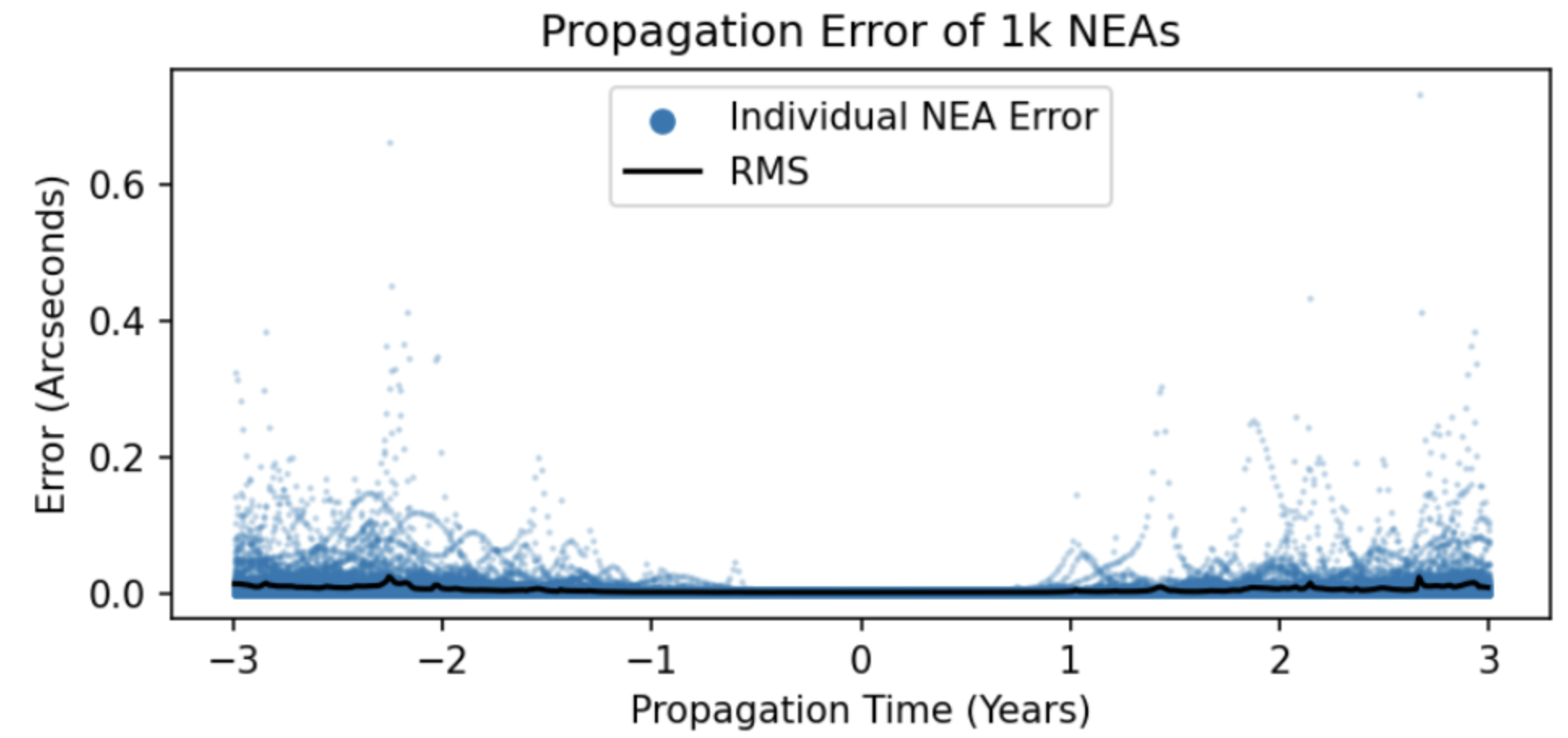
Figure 1: Comparison of NSS-predicted positions for 1000 known NEOs with well-determined orbits (i.e. numbered asteroids) to the JPL Horizons position of each object. The errors for each object are plotted as a blue point at each timestep evaluated. Errors for individual objects will grow well above the RMS value, and then decrease in cases where an object has a close pass with the telescope. The black line shows the RMS error for the population evaluated at each timestep.

4 Comparison to published NEOWISE data

While comparisons of one computer model to another offer an important confirmation that the NSS is correctly computing expected parameters, comparisons to measured data offer an independent means of confirmations of the validity of the methodology. In addition, comparisons to Horizons do not offer the ability to validate the thermal emission model used in the NSS. To address the ability to correctly compute both the ephemerides as well as fluxes, we next performed a validation of the NSS by comparing our predicted results to the reported NEOWISE astrometric and thermal flux measurements that are obtained from the IRSA data archive.

The NEOWISE mission obtained thermal infrared observations of over 150,000 asteroids and comets over the course of its multiple mission phases. The original NEOWISE data (Mainzer et al., 2011a) were obtained as part of the WISE survey (Wright et al., 2010) from 7 January 2010 to 6 August 2010, and simultaneously observed at $3.4~{}\mu$m, $4.6~{}\mu$m, $12~{}\mu$m and $22~{}\mu$m. After the exhaustion of the outer cryogen tank the survey continued in 3-band cryogenic mode though 29 Sep 2010, and then post-cryogenic mode until WISE was put into hibernation on 1 Feb 2011 (Cutri et al., 2012).

NEOWISE reported observations for $428$ NEOs during the fully cryogenic phase of the mission (i.e. when all four channels were operational; Mainzer et al., 2011c). While this population spans the range of magnitudes that we wish to validate here, we desire a larger sample to better investigate any systematics in our flux calculation. To that end, we also consider the $128,462$ Main Belt asteroids that were detected by WISE during the fully cryogenic mission. This population of known objects is used to validate our astrometric computation from a space-based observatory and our calculations of thermal flux.

To check the NSS astrometric accuracy, we downloaded from IRSA the time and pointing of every WISE frameset from the fully cryogenic phase of the mission. We also queried Horizons for the position and velocity of the WISE spacecraft at 15-minute increments over the same time span. These were used in place of the survey pattern and spacecraft ephemerides for NEO Surveyor. Using initial orbits from Horizons for the objects known to have been detected by NEOWISE, we built a model population and used the NSS tools to compute the predicted positions and fluxes for each object.

We compared the positions predicted by the NSS to the measurements reported by the NEOWISE mission to the MPC. We find that every detection that was reported to the MPC was listed as a potential detection by the NSS. Figure 2 shows the offsets between $1,624,795$ predicted and measured on-sky positions for $128,462$ Main Belt asteroids detected in this period. The Main Belt is used here as there are over two orders of magnitude more objects detected than for the NEOs, and it therefore provides superior statistics for constraining the accuracy of our simulation.

The systematic offsets found in this test ($0.05^{\prime\prime}$ and $0.12^{\prime\prime}$ for RA and Dec respectively) are significantly less than the $2.75^{\prime\prime}$ size of a WISE pixel, and the scatter ($2.01^{\prime\prime}$ and $2.10^{\prime\prime}$ 3-sigma in RA and Dec, respectively) is much less than the $7.25^{\prime\prime}$ PSF width. The offsets and scatter also closely match the astrometric residuals for the WISE cryogenic mission recorded by the MPC. These results further demonstrate that the orbit propagation and positional determination in a spacecraft’s field of view has been implemented correctly and with sufficient precision for the needs of the NEOS project.

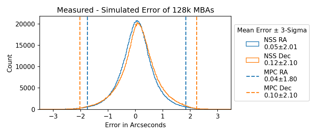
Figure 2: Histogram showing the comparison of NSS-predicted astrometric positions in Right Ascension (blue) and Declination (orange) to the measurements reported to the MPC for $1,624,795$ detections of $128,462$ MBAs observed by NEOWISE during the 2010 fully cryogenic mission. The vertical dashed lines show the offset and $3-\sigma$ scatter provided by MPC’s analysis of observations residuals for the submitted C51 observations to predictions from orbits of known objects. The offsets and random scatter in the observation error from the NSS code are comparable to the values found by the MPC’s analysis.

The vast majority of objects detected by NEOWISE during the cryogenic phase of the mission had sufficient data to fit a thermal model, and thus have physical properties reported (e.g. Mainzer et al., 2011c; Masiero et al., 2011; Mainzer et al., 2019). We take the physical properties for each epoch of observation and use them in the NSS to create a predicted thermal infrared flux at the time of observation. The sensitivity, zero point, and central wavelength for each band are taken from the WISE Explanatory Supplement (Cutri et al., 2012). The predicted value is then compared to the magnitude published for that observation in the NEOWISE data archive in IRSA. This comparison allows us to validate that our thermal modeling code is correctly implemented.

The NEOWISE physical properties were determined by fitting the NEATM thermal model to all detections in a given observing epoch (Mainzer et al., 2011b). The result of this is that the best-fit diameter represents a time-averaged, spherical equivalent size. To properly compare to the observations, we take the average predicted magnitude over each individual observing epoch and compare that to the average of the measured magnitudes at the same epoch. The NEATM beaming parameter used to calculate the flux at each epoch was drawn from the Mainzer et al. (2019) data table. Figure 3 shows the comparison of the predicted and measured magnitudes for the W3 ($12~{}\mu$m) and W4 ($22~{}\mu$m) bands for $1,624,795$ detections of $128,462$ Main Belt asteroids, as these two bands are always thermally dominated for these objects. The shorter wavelength channels can include significant contributions from reflected light depending on object temperature and involve more model-dependent assumptions about the reflected light behavior at these wavelengths and the fractional contributions of each. As above, the Main Belt population was used here to provide robust statistics over the full range of observed magnitudes.

Our analysis shows that the predicted magnitudes generally match the observed values to within the quoted uncertainties. Given that the physical parameters used here were originally derived from WISE data, this demonstrates that the implementation of the model used here is consistent with that used to derive the physical properties. Two exceptions stand out: at the bright end a systematic deviation is seen that is due to incomplete correction of non-linearity and saturation effects in the simulated data, while at the faint end the effects of background noise contributions to the measured data are apparent. This noise effect is especially pronounced in W4, where the multi-band forced-photometry carried out on the WISE images (see Cutri et al., 2012, for details) causes measured values to become brighter than the prediction. This effect occurs because asteroids tend to be brightest in W3, and so a faint W3 source will report a measurement for W4 that is background-dominated and so preferentially brighter than expected. In the regime above the faint limit, the NSS prediction matches the observations, confirming that our implementation of the predicted thermal emission is correct, with a scatter of only $\sim 0.11~{}$mag and systematic offsets well below $0.1~{}$mag.

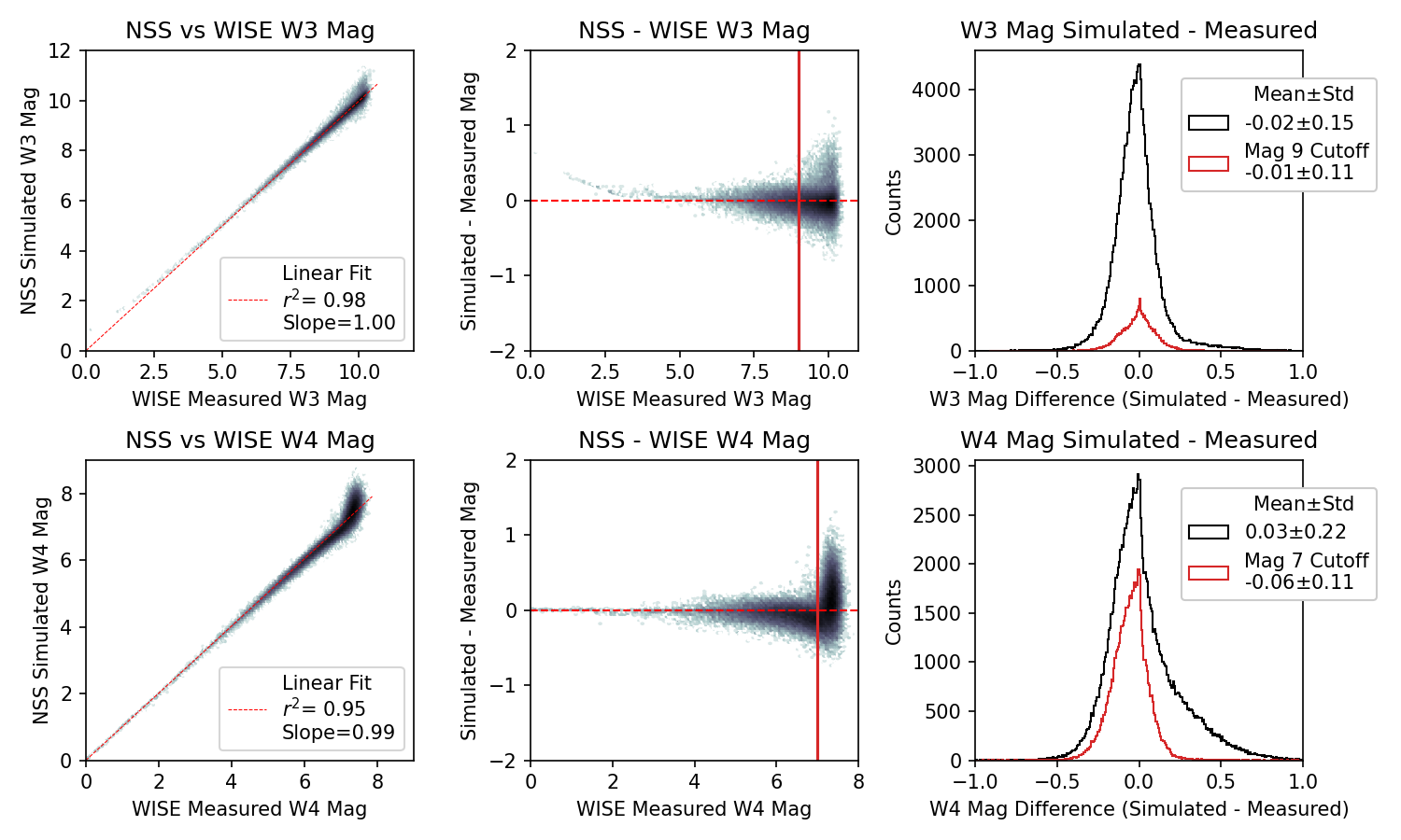
Figure 3: Validation of the NSS thermal model is done through comparison of the predicted magnitude to the WISE-measured magnitudes for W3 (top) and W4 (bottom). Columns show: (left) a density plot of the comparison between the prediction and the measurement in grey along with a best-fit linear trend in red; (middle) a density plot of the measured magnitude against the difference between the simulation and the measurement with the vertical red line showing the approximate transition into a background-impacted regime; (right) histograms of the magnitude differences for all objects in black and those brighter than the background cutoff in red. The spatial bins in the density plots are shaded following a logarithmic scale to emphasize the bright tail.

5 Recovery of new NEOWISE detections of known NEOs

Having demonstrated that the NSS can successfully reproduce the positions and magnitudes of the asteroids already measured by NEOWISE, it becomes natural to ask if this tool can identify detections in the NEOWISE data that have not yet been reported. Searches of NEOWISE data for unreported detections of known NEOs have been successfully conducted in the past (see Mainzer et al., 2014b; Masiero et al., 2018, 2020, for details). However there is a continuing benefit in revised searches of older data as new objects are discovered and known objects receive improved orbital solutions. The new NSS software developed for the NEO Surveyor provides the tools needed to quickly search the entire NEOWISE archive for predicted detections of all known NEOs.

The population we used for our search was drawn from the Minor Planet Center’s MPCORB file, filtered to only include those objects with perihelion distances of $q<1.3~{}$AU. This query was carried out on 17 Aug 2022, and resulted in a list of 29231 objects. Five objects that are listed in the MPCORB catalog but hit the Earth shortly after discovery were filtered from the search; as all of these objects have $H_{V}>29~{}$mag they are almost certainly too small to have been detected by NEOWISE. Objects with short observational arcs were not specifically removed, so that NEOWISE detections close in time to the observed arc might be recovered. These objects will have large positional uncertainties at other times, but visual vetting of recovered detections will remove spurious associations.

For objects where the physical properties were known, we used the measured diameter and albedos for the search. For all other objects we assumed an albedo of $p_{V}=5\%$ and derived a diameter based on the published $H_{V}$ magnitude which will result in the objects being preferentially larger than reality and make the fluxes predicted by the NSS larger. This ensures that our list of potential detections is as comprehensive as possible.

As was done for the test described above, we used the structure of the NSS code to simulate the position and viewing geometry of NEOWISE. The IRSA Single-Exposure Frame Metadata tables for each mission phase were queried without constraint to determine the position of the field of view of each frame with the associated MJD. These then became the “Visits” that would be used by the NSS. The frame metadata tables do not include the spacecraft position, so to calculate that we downloaded from Horizons the position of the WISE spacecraft at 15-minute intervals for the duration of all phases of the mission from 07 Jan 2010 to 13 Dec 2021. These way-points were propagated in time to the center point of each exposure to get the spacecraft position at each Visit.

The state vector for each object was propagated to the time of each exposure, and compared to the field of view of the detectors. Objects that fell on at least one detector were considered Potential Detections. To determine detectability, we convert the magnitude in each band for a signal-to-noise ratio (SNR) of five given in the WISE and NEOWISE Explanatory Supplements (Cutri et al., 2012, 2015) into fluxes, and compare those values to the flux determined for the object using NEATM. All objects passing this threshold were reported by the NSS ($\sim 30,000$ instances per year for the two band data and $\sim 37,000$ instances in the eight months of 4-band and 3-band cryo mission phases).

This list should then include all possible detections of all currently known NEOs during the NEOWISE survey. This output was filtered to remove all detections that had already been reported to the MPC, either those found by the WMOPS automated processing or recovered in previous searched of missed detections ($\sim 11,000$ during the cryo mission phases and $\sim 4,000$ per year for the two-band data). Taking the remaining list of potential detections that were not present in the MPC observation file, we then searched the IRSA archive of each mission phase at the predicted time and position, within 5 arcsecs of the predicted position and 5 seconds of exposure time of the frame. Approximately $70\%$ of potential detections had no associated source returned by IRSA; the most likely cause for this is that real NEOs had higher albedos than our assumed value which would translate to smaller sizes and fainter IR fluxes when using the $H_{V}$ magnitude and an assumed size. This fraction is consistent with the known bias toward higher albedo NEOs for objects discovered by ground-based surveys (Masiero et al., 2020).

The data table files returned by IRSA were cleaned to remove sources of contamination. This included removing sources that were associated with background stars; removing detections that have $rchi2$ data columns larger than three, an indication from the PSF-fit quality measurements that they are likely cosmic rays; and removing detections that had colors consistent with being stellar in nature even if not identified as stars (in this case where $W1-W2<1$, cf. Masiero et al., 2017, for details). At the end of this cleaning process there were 2553 detections from the cryogenic mission phase, 817 from the 3-band cryo phase, 1523 from the post-cryo survey, and $2000-2500$ detections from each year of the NEOWISE Reactivation mission.

For each of the $22,842$ detections left after filtering, we generated a finder chart showing the predicted position overlaid on a cutout of each of the available bands. Every detection was checked by-eye to verify that the source looked reliable and that the measurement was not contaminated by background objects, detector effects, or scattered light. An additional requirement was levied on instances of a single predicted detection for an object, where we required that these cases have a SNR$>5$ detection in at least two bands to help ensure that we were detecting real sources. In total, after by-eye filtering, we recover $21,661$ detections of near Earth asteroids that were previously not reported to the MPC. When combined with all previous NEO detections reported to the MPC we now have NEOWISE observations of 3330 NEOs, representing over $10\%$ of all known NEOs.

Detections were broken up into epochs of observation, defined as coherent sets of observations with at least three days of gap between the last detection of one epoch and the first detection of the next. A small number of objects had on-sky motions comparable to the progression of the survey field of regard, resulting in hundreds of detections spanning over a month. In these cases epochs were defined as lasting no longer than 10 days to minimize the changes of viewing geometry during an epoch, and detections were split up to match this requirement.

Of these $21,661$ new detections, $10,939$ are additional detections of an epoch of observation that had already been reported to the MPC. In these cases, either the detection fell just below the signal-to-noise threshold used for tracklet construction in the original WMOPS search, the detection was removed from consideration by WMOPS due to proximity to a nearby inertial source, or the detection links together other WMOPS-reported tracklets. This latter case most often happened when an object was in the NEOWISE field of regard for a long period of time and as such had significant curvature of motion on-sky which resulted in WMOPS splitting the object into separate tracklets.

The remaining recovered detections fall into two groups. The first group contains $5,160$ detections of $1,166$ objects for which no previous NEOWISE measurements had been reported to the MPC. Of these, $768$ tracklets had fewer than five detections, and so would not be found by WMOPS, which requires at least five detections to build a tracklet. An example of this is given in Figure 4, which shows two NEOWISE observations taken 11 second apart of the NEO 2020 TK₃ from the 7th year of the Reactivation Survey, which had an on-sky rate of motion of $70.5~{}$deg/day at the time of observation. $105$ of these objects with previously unreported astrometry ($355$ detections) were included in the physical property analysis conducted by Mainzer et al. (2014b) but not reported to the MPC. Figure 5 shows the distribution of tracklet lengths of these previously unreported objects. The remaining $5,562$ detections represent new observation epochs of $786$ previously-reported objects.

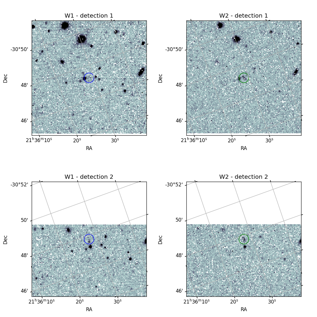
Figure 4: Detections of Near Earth Object 2020 TK₃ in the NEOWISE-Reactivation Year 7 data that were identified by the NSS. This object was seen in two sequential image sets (top and bottom) with center times separated by only 11 seconds. The left and right columns show the W1 and W2 images for each detection, respectively, and the NSS-predicted position for the object is marked by the colored circle overlaid on each image. The object was moving at $70.5~{}$ deg/day at the time of observation; it is noticeably trailed in the $7.7~{}$second-long W2 exposures and motion with respect to the background is apparent. Detection 2 is near the edge of the field of view, resulting in the image being cut off in the figure.

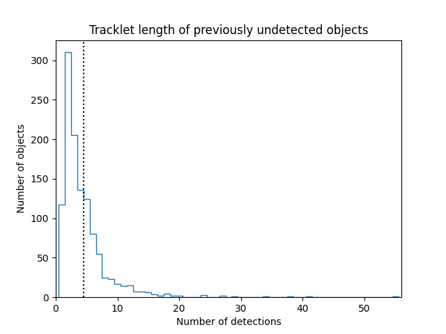
Figure 5: Length of tracklets found in our search of NEOWISE data for objects that had no previously reported measurements. The majority have less than five detections (left of the dotted line) and could not have been found by the automated processing. The longest tracklet here is 55 detections, for object 2017 SG14.

We show in Fig 6 the count newly recovered epochs of NEO detections as a function of time, splitting out objects detected in only a single image with those seen in multiple images. While the detection count shows some structure, it overall is relatively flat. The apparent structures seen in this histogram are:

• The $\sim 3-$year gap readily apparent is due to the period of time when the WISE spacecraft was placed in hibernation, from 1 Feb 2011 until the survey resumed on 13 Dec 2013 (Mainzer et al., 2014a).

• The 2010 period shows a larger number of recovered detections than later times; this is due to two primary effects: 1) WISE was more sensitive to asteroids during the cryogenic portions of the mission and 2) detections identified and used for thermal fitting by Mainzer et al. (2014b) were not reported to the MPC and so will be included in the new detection counts shown here.

• For the data collected after 2013, there appears to be a slight increasing trend in the number of recovered epochs with time. This is consistent with increase in NEO detection rate by ground-based surveys during this time, as the period around discovery is the most likely time for a close, bright pass with the Earth and thus a detection by NEOWISE.

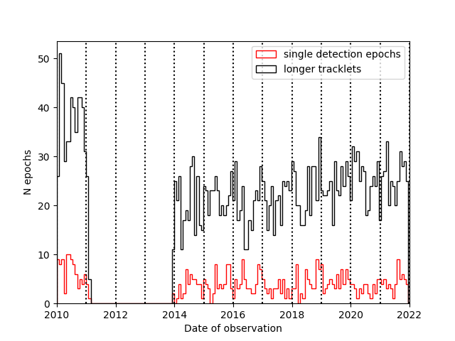
Figure 6: Histogram showing the number of epochs of new detections recovered as a function of time. The binsize used is 28 days, and the vertical dotted lines mark Jan 1 for each year starting with 2010. The red histogram shows epochs that consist of only a single detection, while the black histogram is all other recovered epochs. The large gap from 2011-2014 is the time when the WISE spacecraft was in hibernation. The recovery rate is higher during the cryogenic phase as the telescope was more sensitive then, and because the astrometry for the objects recovered by Mainzer et al. (2014b) was not submitted to the MPC and so does not appear in the list of already-reported detections. The general trend of increasing epochs with time during the reactivation mission is a result of the increasing number of objects discovered by ground-based surveys.

The recovered NEO detections found in this search show no significant trend with on-sky position. The distribution of declinations follows the expected $\cos\left({\rm Dec}\right)$ behavior and the distribution of Right Ascensions is flat. This holds for both the single-detection epochs as well as the longer tracklet epochs. The recovered detections are also uniform with respect to ecliptic and galactic coordinates as well. All detections recovered as part of this search were reported to the MPC on 2023 Feb 27 and were published in MPEC 2023 E12.

6 Discussion

The analysis presented here demonstrates that the new software tools developed for the NEOS mission survey simulator are performing as expected. This result establishes a high level of confidence in the outputs of the simulation in terms of the expected survey completeness. While the top-level mission requirement for NEO Surveyor is to detect two-thirds of the potentially hazardous asteroids, demonstrating this using the known population requires an a priori knowledge of the population size and properties. Once NEO Surveyor launches, the NSS code will use the synthetic population model to evaluate the survey performance in real-time by tracking the completeness NEO Surveyor would have achieved on the synthetic population. Simultaneously, the NSS provides the tools needed to conduct a full population debiasing at the end of the survey for the NEOs. In this way, the survey goals can be doubly-confirmed.

Survey simulation tools like the NSS are necessary for fully understanding the impacts of design choices on the goals of a survey. By designing the NSS to be generalizable it is possible to simulate other surveys and other populations, as we have done here for the NEOWISE survey. Grav et al. (2023) demonstrate a different use case for the NSS, where they simulated the historical sensitivity of ground-based surveys to reproduce the NEO discovery rate to the present day in order to quantify the fraction of objects in our simulated population that would be expected to be present in the NEO catalog once NEO Surveyor launches. In this way we can determine the overall catalog completeness for PHAs from the worldwide NEO search efforts.

7 Conclusions

The NEO Surveyor mission has developed computational tools to simulate the observations to be conducted as a way of assessing total expected performance for the mission. We have demonstrated here through comparisons to JPL Horizons, the MPC, and NEOWISE measurements that the various components of the NSS are functioning as expected and producing correct positions and fluxes. This external validation is critical to establishing the confidence in the expected survey completeness that NEO Surveyor will deliver.

In addition to this validation analysis, we also use these tools to search for previously missed detections of NEOs in the NEOWISE data. We find $21,661$ detections that were previously unreported, which we have now submitted to the MPC, including data on $1166$ NEOs that previously had no reported NEOWISE observations. Many of these detections were either extensions of previously reported tracklets that had been discarded due to filtering of nearby background objects, while the others were detections of objects that did not meet the criteria for tracklet construction used by the NEOWISE automated processing. As powerful new software tools like the NSS become available, searches of data archives like NEOWISE are expected to continue providing important data that was previously unrecognized for many years to come. This trend will likely accelerate as the next generation surveys find orders of magnitude more objects that can be the basis of future precovery efforts.

References

- Bowell et al. (1989) Bowell E., Hapke B., Domingue D., et al., 1989, Asteroids II (R. P. Binzel et al., eds), Univ. of Arizona Press, 524.
- Cutri et al. (2012) Cutri, R.M., Wright, E., Conrow, T., Bauer, J., et al., 2012, Explanatory Supplement to the WISE All-Sky Data Release Products, https://wise2.ipac.caltech.edu/docs/release/allsky/expsup
- Cutri et al. (2015) Cutri, R.M., Mainzer, A., Conrow, T., Masci, F., Bauer, J., et al., 2015, Explanatory Supplement to the NEOWISE Data Release Products, https://wise2.ipac.caltech.edu/docs/release/neowise/expsup
- Grav et al. (2023) Grav, T., et al., 2023, PSJ, submitted.
- Harris et al. (1998) Harris, A.W., 1998, Icarus, 131, 291.
- Lebofsky et al. (1978) Lebofsky, L. A., Veeder G. J., Lebofsky M. J., and Matson D. L., 1978, Icarus, 35, 336.
- Mainzer et al. (2011a) Mainzer, A.K., Bauer, J.M., Grav, T., Masiero, J., et al., 2011a, ApJ, 731, 53.
- Mainzer et al. (2011b) Mainzer, A.K., Grav, T., Masiero, J., et al., 2011b, ApJ, 736, 100.
- Mainzer et al. (2011c) Mainzer, A.K., Grav, T., Bauer, J.M., Masiero, J., et al., 2011c, ApJ, 743, 156.
- Mainzer et al. (2014a) Mainzer, A.K., Bauer, J., Cutri, R., Grav, T., Masiero, J., et al., 2014a, ApJ, 792, 30.
- Mainzer et al. (2014b) Mainzer, A.K., Bauer, J., Grav, T., Masiero, J., Cutri, R., et al., 2014b, ApJ, 784, 110.
- Mainzer et al. (2019) Mainzer, A.K., Bauer, J., Cutri, R., et al., 2019, NASA Planetary Data System. doi:10.26033/18S3-2Z54
- Mainzer et al. (2023) Mainzer, A.K., et al., 2023, PSJ submitted.
- Masiero et al. (2011) Masiero, J.R, Mainzer, A.K., Grav, T., et al., 2011, ApJ, 741, 68.
- Masiero et al. (2017) Masiero, J.R, Nugent, C., Mainzer, A.K., Wright, E., Bauer, J., et al., 2017, AJ, 154, 168.
- Masiero et al. (2018) Masiero, J.R, Redwing, E., Mainzer, A.K., Bauer, J.M., Cutri, R.M., et al., 2018, AJ, 156, 60.
- Masiero et al. (2020) Masiero, J.R, Smith, P., Teodoro, L., et al., 2020, PSJ, 1, 9.
- Wright (2005) Wright, E.L., 2005, New Astronomy Reviews, 49, 407.
- Wright et al. (2010) Wright, E.L., Eisenhardt, P., Mainzer, A.K., Ressler, M.E., Cutri, R.M., et al., 2010, AJ, 140, 1868.