STANLEY: Stochastic Gradient Anisotropic
Langevin Dynamics for Learning Energy-Based Models
Abstract
We propose in this paper, STANLEY, a STochastic gradient ANisotropic LangEvin dYnamics, for sampling high dimensional data.
With the growing efficacy and potential of Energy-Based modeling, also known as non-normalized probabilistic modeling, for modeling a generative process of different natures of high dimensional data observations, we present an end-to-end learning algorithm for Energy-Based models (EBM) with the purpose of improving the quality of the resulting sampled data points.
While the unknown normalizing constant of EBMs makes the training procedure intractable, resorting to Markov Chain Monte Carlo (MCMC) is in general a viable option.
Realizing what MCMC entails for the EBM training, we propose in this paper, a novel high dimensional sampling method, based on an anisotropic stepsize and a gradient-informed covariance matrix, embedded into a discretized Langevin diffusion.
We motivate the necessity for an anisotropic update of the negative samples in the Markov Chain by the nonlinearity of the backbone of the EBM, here a Convolutional Neural Network.
Our resulting method, namely STANLEY, is an optimization algorithm for training Energy-Based models via our newly introduced MCMC method.
We provide a theoretical understanding of our sampling scheme by proving that the sampler leads to a geometrically uniformly ergodic Markov Chain.
Several image generation experiments are provided in our paper to show the effectiveness of our method.
1 Introduction
The modeling of a data generating process is critical for many modern learning tasks. A growing interest in generative models within the realm of computer vision has led to multiple interesting solutions. In particular, Energy-based models (EBM) (Zhu et al., 1998; LeCun et al., 2006), are a class of generative models that learns high dimensional and complex (in terms of landscape) representation/distribution of the input data. EBMs have been used in several applications including computer vision (Ngiam et al., 2011; Xie et al., 2016; Du and Mordatch, 2019), natural language processing (Mikolov et al., 2013; Deng et al., 2020), density estimation (Li et al., 2019; Song et al., 2019) and reinforcement learning (Haarnoja et al., 2017). Formally, EBMs are built upon an unnormalized log probability, called the energy function, that is not required to sum to one as standard log probability functions. This noticeable feature allows for more freedom in the way one parameterizes the EBM. For instance, Convolutional Neural Network can be employed to parameterize this function, see Xie et al. (2016).
The training procedure of such models consists of finding an energy function that assigns to lower energies to observations than unobserved points. This phase can be cast as an optimization task and several ways are possible to solve it. In this paper, we will focus on training the EBM via Maximum Likelihood Estimation (MLE). Particularly, while using MLE to fit the EBM on observed data, the high non-convexity of the loss function leads to a non closed form maximization step. In general, gradient based optimization methods are thus used during that phase. Besides, given the intractability of the normalizing constant of our model, the aforementioned gradient, which is an intractable integral, needs to be approximated. A popular and efficient way to conduct such approximation is to use Monte Carlo approximation where the samples are obtained via Markov Chain Monte Carlo (MCMC) (Meyn and Tweedie, 2012). The goal of this embedded MCMC procedure while training the EBM is to synthesize new examples of the input data and use them to approximate quantities of interest.
Hence, the sampling phase is crucial for both the EBM training speed and its final accuracy in generating new synthetic samples. The computational burden of those MCMC transitions, at each iteration of the EBM training procedure, is alleviated via different techniques in the literature. For instance, in Nijkamp et al. (2019), the authors develop a short-run MCMC as a flow-based generator mechanism despite its non convergence property. Other principled approach, as in Hinton (2002), keeps in memory the final chain state under the previous global model parameter and uses it as the initialization of the current chain. The heuristic of such approach is that along the EBM iterations, the conditional distributions, depending on the model parameter, are more and more similar and thus using a good sample from the previous chain is in general a good sample of the current one. Though, this method can be limited during the first iterations of the EBM training since when the model parameter changes drastically, the conditional distributions do change too, and samples from two different chains can be quite inconsistent. Several extensions modifying the way the chain is initialized can be found in Welling and Hinton (2002); Gao et al. (2018); Du and Mordatch (2019).
An interesting line of work in the realm of MCMC-based EBM tackles the biases induced by stopping the MCMC runs too early. Indeed, it is known, see Meyn and Tweedie (2012), that before convergence, MCMC samples are biased and thus correcting this bias while keeping a short and less expensive run is an appealing option. Several contributions aiming at removing this bias for improved MCMC training include coupling MCMC chains, see Qiu et al. (2020); Jacob et al. (2020) or simply estimating this bias and correct the chain afterwards, see Du et al. (2021).
Here, our work is in line with the context of – high-dimensional data, – EBM parameterized by deep neural networks and – MLE-based optimization via MCMC, which make our method particularly attractive to all of the above combined. We also consider the case of a short-run MCMC for the training of an EBM. Rather than focusing on debiasing the chain, we develop a new sampling scheme where the goal is to obtain better samples from the target distribution in fewer MCMC transitions. We consider that the shape of the target distribution, which inspires our proposed method, is of utmost importance to obtain such negative samples. Our contributions are summarized below:
-
1.
We develop STANLEY, an Energy-Based model training method that embeds a newly proposed convergent and efficient MCMC sampling scheme, focusing on curvature informed metrics of the target distribution one wants to sample from.
-
2.
Based on an anisotropic stepsize, our method, which is an improvement of the Langevin Dynamics, achieves to obtain negative samples from the Energy-Based model data distribution and improves the overall optimization algorithm.
-
3.
We prove the geometric ergodicity uniformly on any compact set of our MCMC method assuming some regularity conditions on the target distribution and on the backbone model of the EBM.
-
4.
We empirically assess the effectiveness of our method on several image generation tasks, both on synthetic and real datasets including the Oxford Flowers 102 dataset, CIFAR-10 and CelebA. We conclude the work with an Image inpainting experiment on a benchmark dataset.
Roadmap. Section 2 introduces important notations and related work. Section 3 develops the main algorithmic contribution of this paper, namely STANLEY. Section 4 presents our main theoretical results focusing on the ergodicity of the proposed MCMC sampling method. Section 5 presents several image generation experiments on both synthetic and real datasets. The complete proofs of our theoretical results can be found in the supplementary material.
2 On MCMC-based Energy Based Models
Given a stream of input data noted , the EBM is a Gibbs distribution defined as follows:
| (1) |
where denotes the global parameters vector of our model and is the normalizing constant (with respect to ). In particular, , is the energy function (up to a sign) that can be parameterized by a Convolutional Neural Network for instance. The natural way of fitting model (1) is to employ Maximum Likelihood Estimation (MLE) maximizing the marginal likelihood , i.e., finding the vector such that for any ,
| (2) |
where denotes the true distribution of the input data . The optimization task (2) is not tractable in closed form and requires an iterative procedure in order to be solved. The standard algorithm used to train EBMs is Stochastic Gradient Descent (SGD), see Robbins and Monro (1951); Bottou et al. (2007). SGD requires having access to the gradient of the objective function which requires computing an intractable integral, due to the high nonlinearity of the generally utilized parameterized model . Given the general form defined in (1), we have that:
and a simple Monte Carlo approximation of yields the following expression of the gradient
| (3) |
where are samples obtained from the EBM and are drawn uniformly from the true data distribution . While drawing samples from the data distribution is trivial, the challenge during the EBM training phase is to obtain samples from the EBM distribution for any model parameter . This task is generally performed using MCMC methods. State-of-the-art MCMC used in the EBM literature include Langevin Dynamics, see Grenander and Miller (1994); Roberts and Rosenthal (1998); Roberts and Tweedie (1996) and Hamiltonian Monte Carlo (HMC), see Neal (2011). Those methods are detailed in the sequel and are important concepts of our contribution.
Energy Based Models. Energy based models are a class of generative models that leverage the power of Gibbs potential and high dimensional sampling techniques to produce high quality synthetic image samples. EBMs are powerful tools for generative modeling tasks, as a building block for a wide variety of tasks. The main purpose of EBMs is to learn an energy function (1) that assigns low energy to a stream of observation and high energy values to other inputs. Learning of such models is done via MLE (Xie et al., 2016; Du and Mordatch, 2019) or Score Matching (Hyvärinen, 2005) or Noise Constrastive Estimation (Gao et al., 2020). In several general applications, authors leverage the power of EBMs for develop an energy-based optimal policy where the parameters of that energy function are provided by the reward of the overall system. Learning EBMs with alternative strategies include contrastive divergence (CD) (Hinton, 2002; Tieleman, 2008), noise contrastive estimation (NCE) (Gutmann and Hyvärinen, 2010; Gao et al., 2020), introspective neural networks (INN) (Lazarow et al., 2017; Jin et al., 2017; Lee et al., 2018), cooperative networks (CoopNets) (Xie et al., 2018a, 2020, 2021c, 2022a, 2022c; Zhao et al., 2023), f-divergence (Yu et al., 2020), and triangle divergence (Han et al., 2019, 2020). Recently, EBMs parameterized by modern neural networks have drawn much attention from the computer vision and machine learning communities. Successful applications with EBMs include image generation (Xie et al., 2016; Gao et al., 2018; Du and Mordatch, 2019; Zhao et al., 2021; Zheng et al., 2021), videos (Xie et al., 2017, 2021d), 3D volumetric shapes (Xie et al., 2018b, 2022b), unordered point clouds (Xie et al., 2021a), texts (Deng et al., 2020), molecules (Ingraham et al., 2019; Du et al., 2020), as well as image-to-image translation (Xie et al., 2022a, 2021b), unpaired cross-domain image translation (Xie et al., 2021b; Song et al., 2023), out-of-distribution detection (Liu et al., 2020), inverse optimal control (Xu et al., 2022), deep regression (Gustafsson et al., 2020), salient object detection (Zhang et al., 2022) and latent space modeling (Pang et al., 2020; Zhang et al., 2021, 2023). Yet, unlike VAE (Kingma and Welling, 2014) or GAN (Goodfellow et al., 2014) EBMs enjoy from a single structure requiring training (versus several networks) resulting in more stability. The use of implicit sampling techniques, such as MCMC, as detailed in the sequel, allows more flexibility by trading off sample quality for computation time. Overall, the implicit property of the EBM, seen as an energy function, makes it a tool of choice as opposed to explicit generators that are limited to some design choices, such as the choice of the prior distribution for VAEs or both neural networks design in GANs.
MCMC procedures. Whether for sampling from a posterior distribution (Robert et al., 2010; Han et al., 2017; Xie et al., 2019; Zhang et al., 2020; An et al., 2021; Zhu et al., 2023; Xie et al., 2023), or in general intractable likelihoods scenario (Doucet et al., 2000), various inference methods are available. Approximate inference is a partial solution to the inference problem and include techniques such as Variational Inference (VI) (Wainwright and Jordan, 2008; de Freitas et al., 2001) or Laplace Approximation (Wolfinger, 1993; Rue et al., 2009). Those methods allow the simplification of the intractable quantities and result in the collection of good, yet approximate, samples. As seen in (3), training an EBM requires obtaining samples from the model itself. Given the nonconvexity of the structural model with respect to the model parameter , direct sampling is not an option. Besides, in order to update the model parameter , usually through gradient descent type of methods (Bottou et al., 2007), exact samples from the EBM are needed in order to compute a good approximation of its (intractable) gradient, see (3). To do so, we generally have recourse to MCMC methods. MCMC are a class of inference algorithms that provide a principled iterative approach to obtain samples from any intractable distribution. While being exact, the samples generally represent a larger computation burden than methods such as VI. Increasing the efficiency of MCMC methods, by obtaining exact samples, in other words constructing a chain that converges faster, in fewer transitions is thus of utmost importance in the context of optimizing EBMs. Several attempts have been proposed for the standalone task of posterior sampling through the use of Langevin diffusion, see the Unadjusted Langevin in Brosse et al. (2019), the MALA algorithm in Roberts and Rosenthal (1998); Roberts and Tweedie (1996); Durmus et al. (2017) or leveraging Hamiltonian Dynamics as in Girolami and Calderhead (2011). We propose in the next section, an improvement of the Langevin diffusion with the ultimate goal of speeding the EBM training procedure. Our method includes this latter improvement in an end-to-end learning algorithms for Energy-Based models.
3 Gradient Informed Langevin Diffusion
We now introduce the main algorithmic contribution of our paper, namely STANLEY. STANLEY is a learning algorithm for EBMs, comprised of a novel MCMC method for sampling samples from the intractable model (1). We provide theoretical guarantees of our scheme in Section 4.
3.1 Preliminaries on Langevin MCMC based EBM
State-of-the-art MCMC sampling algorithm, particularly used during the training procedure of EBMs, is the discretized Langevin diffusion, cast as Stochastic Gradient Langevin Dynamics (SGLD), see Welling and Teh (2011). In particular, several applications using EBM and SGLD have thrived in image generation, natural language processing or even biology (Du et al., 2020). Yet, the choice of the proposal, generally Gaussian, is critical for improving the performances of both the sampling step (inner loop of the whole procedure) and the EBM training. We recall the vanilla discretized Langevin diffusion used in the related literature as follows:
where is the target potential one needs samples from and defined in (1), represents the states of the chains at iteration , i.e., the generated samples in the context of EBM, is the MCMC iteration index and is the Brownian motion, usually set as a Gaussian noise and which can be written as where is a standard Gaussian random variable and is a scaling factor for implementation purposes. This method directs the proposed moves towards areas of high probability of the stationary distribution , for any , using the gradient of and has been the object of several studies (Girolami and Calderhead, 2011; Cotter et al., 2013). In high dimensional and highly nonlinear settings, the burden of computing this gradient for a certain number of MCMC transitions leads to a natural focus: improving of the sampling scheme by assimilating information about the landscape of the target distribution while keeping its ease of implementation.
3.2 STANLEY, an Anisotropic Energy Based Modeling Approach
Given the drawbacks of current MCMC methods used for training EBMs, we introduce a new sampler based on the Langevin updates presented above in Step 4 of Algorithm 1.
| (4) |
| (5) |
Intuitions behind the efficacy of STANLEY: Some past modifications have been proposed in particular to optimize the covariance matrix of the proposal of the general MCMC procedure in order to better stride the support of the target distribution. Langevin Dynamics is one example of those improvements where the proposal is a Gaussian distribution where the mean depends on the gradient of the log target distribution and the covariance depends on some Brownian motion. For instance, in Atchadé (2006); Marshall and Roberts (2012), the authors propose adaptive and geometrically ergodic Langevin chains. Yet, one important characteristic of our EBM problem, is that for each model parameter updated through the training iterations, the target distribution moves and the proposal should take that adjustment into account. The techniques in Atchadé (2006); Marshall and Roberts (2012) does not take the whole advantage of changing the proposal using the target distribution. In particular, the covariance matrix of the proposal is given by a stochastic approximation of the empirical covariance matrix. This choice seems completely relevant as soon as the convergence towards the stationary distribution is reached, in other words it would make sense towards the end of the EBM training, as the target distributions from a model parameter to the next one are similar. However, it does not provide a good guess of the variability during the first iterations since it is still very dependent on the initialization.
Moreover, in Girolami and Calderhead (2011), the authors consider the approximation of a constant. Even though this simplification leads to ease of implementation, the curvature metric chosen by the authors need to be inverted, step that can be a computational burden if not intractable. Especially in the case we are considering in our paper, i.e., ConvNet-based EBM, where the high nonlinearity would lead to intractable expectations. Therefore, in (4) and (5) of Algorithm 1, we propose a variant of Langevin Dynamics, in order to sample from a target distribution, using a full anisotropic covariance matrix based on the anisotropy and correlations of the target distribution, see the erm.
4 Geometric Ergodicity of STANLEY
We will present our theoretical analysis for the Markov Chain constructed using Line 3-4 of Algorithm 1. Let be a subset of for some integer . We denote by the measurable space of for some integer . We define a family of stationary distribution , probability density functions with respect to the Lebesgue measure on the measurable space . This family of p.d.f. defines the stationary distributions of our newly introduced sampler.
4.1 Notations and Assumptions
For any chain state , we denote by the transition kernel as defined in the STANLEY update in Line 4 of Algorithm 1. The objective of this section is to rigorously show that each transition kernel , for any parameter is geometrically ergodic and that this result holds for any compact subset . As a background note, a Markov chain, as constructed Line 4, is said to be geometrically ergodic when iterations of the same transition kernel is converging to the stationary distribution of the chain with a geometric dependence on .
As in Allassonniere and Kuhn (2015), we state the assumptions required for our analysis. The first one is related to the continuity of the gradient of the log posterior and the unit vectors pointing in the direction of the sample and in the direction of the gradient of the log posterior distribution at :
H 1.
For all , the structural model satisfies:
Besides, we assume some regularity conditions of the stationary distributions with respect to :
H 2.
and are continuous on .
For a positive and finite function noted , we define the V-norm distance between two arbitrary transition kernels and as follows:
The definition of this norm allows us to establish a convergence rate for our sampling method by deriving an upper bound of where denotes the number of MCMC transitions. We recall that is the transition kernel defined by Line 4 of Algorithm 1 and is the stationary distribution of our Markov chain at a given EBM model . This quantity characterizes how close to the target distribution our chain is getting, after a finite time of iterations and will eventually formalize the V-uniform ergodicity of our method. We specify that strictly speaking, is a probability measure, and not a transition kernel. However is well-defined if we consider as a kernel:
Here, for some we define the function, also know as the drift, for all as follows:
| (6) |
where is a constant, with respect to the chain state , such that for all , . Note that the V norm depends on the chain state noted and of the global model parameter varying through the optimization procedure. Yet, in both main results, the ergodicity and the convergence rate, including the underlying drift condition, are established uniformly on the parameter space . We also define the auxiliary functions, independent of the parameter as:
| (7) |
and assume the following:
H 3.
There exists a constant such that for all and , the function , defined in (7), is integrable against the kernel and we have
4.2 Convergence Results
The result consists in showing V-uniform ergodicity of the chain, the irreducibility of the transition kernels and their aperiodicity, following Meyn and Tweedie (2012); Allassonniere and Kuhn (2015). We also prove a drift condition which states that the transition kernels tend to bring back elements into a small set. Then, V-uniform ergodicity of the transition kernels boils down from the latter proven drift condition.
Important Note: The stationary distributions depend on as they vary at each model update during the EBM optimization phase. Thus uniform convergence of the chain is important in order to characterize the sampling phase throughout the entire training phase. Particularly at the beginning, the shape of the distributions one needs to sample from varies a lot from a parameter to another.
Theorem 4.2 shows two important convergence results for our sampling method. First, it establishes the existence of a small set leading to the crucially needed aperiodicity of the chain and ensuring that each transition moves towards a better state. Then, it provides a uniform ergodicity result of our sampling method in STANLEY, via the so-called drift condition providing the guarantee that our transition kernels attract the states into the small set . Moreover, the independence on the EBM model parameter of in (9) leads to uniform ergodicity as shown in the Corollary 4.2.
Assume H1-H3. For any , there exists a drift function , a set , a constant such that
| (8) |
Moreover there exists , and a drift function , independent of such that for all :
| (9) |
Assume H1-H3. A direct consequence of Theorem 4.2 is that the family of transition kernels are uniformly ergodic,i.e., for any compact , there exist constants and such for any MCMC iteration ,we have:
| (10) |
where is the drift function in Theorem 4.2 and is any bounded function we apply a transition to. While Theorem 4.2 is critical for proving the aperiodicity and irreducibility of the chain, we establish the geometric convergence speed of the chain. We do not only show the importance of the uniform ergodicity of the chain, which makes it appealing for the EBM training since the model parameter is often updated, but we also derive a geometrical rate in Corollary 4.2.
We encourage the readers to read through the sketch of the main Theorem of our paper provided on the first page of the supplemental as we give the important details leading to the desired ergodicity results. Those various techniques are common in the MCMC literature and we refer the readers to several MCMC handbooks such as Neal (2011); Meyn and Tweedie (2012) for more understanding.
5 Numerical Experiments
We conduct a collection of experiments to show the effectiveness of our method, both on synthetic and real datasets. After verifying the advantage of STANLEY on a Gaussian Mixture Model (GMM) retrieving the synthetic data observations, we then investigate its performance when learning a distribution over high-dimensional natural images such as pictures of flowers, see the Flowers dataset in Nilsback and Zisserman (2008), or general concepts featured in CIFAR-10 (Krizhevsky and Hinton, 2009). For both methods, we use the Frechet Inception Distance (FID), as a reliable performance metrics as detailed in Heusel et al. (2017). In the sequel, we tune the learning rates over a fine grid and report the best result for all methods. For our method STANLEY, the threshold parameter th, crucial for the implementation of the stepsize (4) is tuned over a grid search as well. As mentioned above, we also define a Brownian motion as , and tune the scaling factor for better performances.
5.1 Toy Example: Gaussian Mixture Model
Datasets. We first demonstrate the outcomes of both methods including our newly proposed STANLEY for low-dimensional toy distributions. We generate synthetic 2D rings data and use an EBM to learn the true data distribution and put it to the test of generating new synthetic samples.
Methods and Settings. We consider two methods. Methods are ran with nonconvergent MCMC, i.e.,, we do not necessitate the convergence to the stationary distribution of the Markov chains. The number of transitions of the MCMC is set to per EBM iteration. We use a standard deviation of as in Nijkamp et al. (2020). Both methods have a constant learning rate of . The value of the threshold th for our STANLEY method is set to . The total number of EBM iterations is set to . The global learning rate is set to a constant equal to .
Network architectures. For the backbone of the EBM model, noted in (1), we chose a CNN of 2D convolutional layers and Leaky ReLU activation functions, with the leakage parameter set to . The number of hidden neurons varies between and .
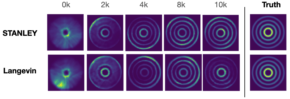
Results. We observe Figure 1 the outputs using both methods on the toy dataset. While they achieve a great representation of the truth after a large number of iterations, we notice that STANLEY learns an energy that closely approximates the true density during the first thousands of iterations if the training process. The sharpness of the data generated by STANLEY in the first iterations shows an empirically better ability to sample from the 2D dataset.
5.2 Image Generation
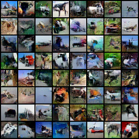
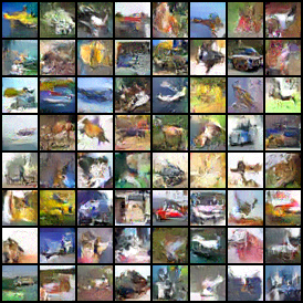
Datasets. We run our method and several baselines detailed below on the CIFAR-10 dataset (Krizhevsky and Hinton, 2009) and the Oxford Flowers 102 dataset (Nilsback and Zisserman, 2008). CIFAR-10 is a popular computer-vision dataset of training images and test images, of size . It is composed of tiny natural images representing a wide variety of objects and scenes, making the task of self supervision supposedly harder. The Oxford Flowers 102 dataset is composed of 102 flower categories. Per request of the authors, the images have large scale, pose and light variations making the task of generating new samples particularly challenging.
Methods and Settings for the Flowers dataset. Nonconvergent MCMC are also used in this experiment and the number of MCMC transitions is set to . Global learning parameters of the gradient descent update is set to for both methods. We run each method during iterations and plot the results using the final vector of fitted parameters.
Methods and Settings for CIFAR-10. We employ the same nonconvergent MCMC strategies for this experiment. The value of the threshold th for our STANLEY method is set to . The total number of EBM iterations is set to . The global learning rate is set to a constant equal to . In this experiment, we slightly change the last step of our method in Algorithm 1. Indeed, Line 11 in Algorithm 1 is not a plain Stochastic Gradient Descent here but we rather use the Adam optimizer (Kingma and Ba, 2015). The scaling factor of the Brownian motion is .
Network architectures for both. The backbone of the energy function for this experiment is a vanilla ConvNet composed of convolution layers with stride . Convolutional Layers using ReLU activation functions are stacked.
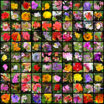
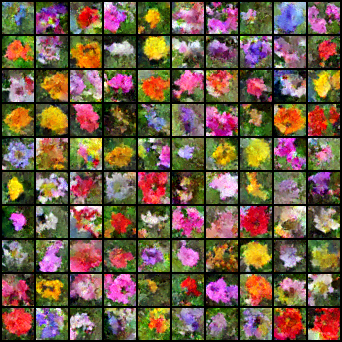
Results. (Flowers) Visual results are provided in Figure 2 where we have used both methods to generate synthetic images of flowers. For each threshold iterations number ( iterations) we sample synthetic images from the EBM model under the current vector of parameters and use the same number of data observations to compute the FID similarity score as advocated in Heusel et al. (2017). The evolution of the FID values are reported in Figure 3 (Left) through the iterations. We note that our method outperforms the other baselines for all iterations threshold, including the Vanilla Langevin (in blue) which is an ablated form our STANLEY (no adaptive stepsize).
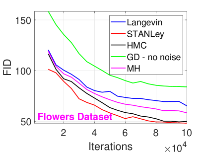
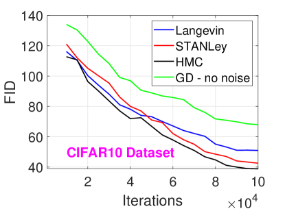
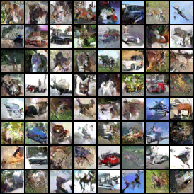
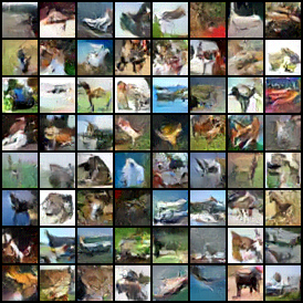
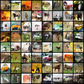
(CIFAR-10) Visual results are provided in Figure 4 where we have used both methods to generate synthetic images of flowers. The FID values are reported in Figure 3 (Right) and have been computed using synthetic images from each model. The similarity score is then evaluated every iterations. While the FID curves for the Flowers dataset exhibits a superior performance of our method throughout the training procedure, we notice that in the case of CIFAR-10, vanilla method seems to be slightly better than STANLEYḋuring the first iterations, i.e., when the model is still learning the representation of the images. Yet, after a certain number of iterations, we observe that STANLEY leads to more accurate synthetic images. This behavior can be explained by the importance of incorporating curvature informed metrics into the training process when the parameter reaches a neighborhood of the solution.
5.3 Image Inpainting
The image inpainting experiment aims to fill missing regions of a damaged image with synthesized content.
Datasets. We use the CelebA dataset (Liu et al., 2015) to evaluate our learning algorithm, which contains more than 200k RGB color facial image. We use 100k images for training and 100 images for testing.
Methods and Settings. Nonconvergent MCMC are also used in this experiment and the number of MCMC transitions is set to . Global learning parameters of the gradient descent update is set to . We run each method during iterations and plot the results using the final vector of fitted parameters.
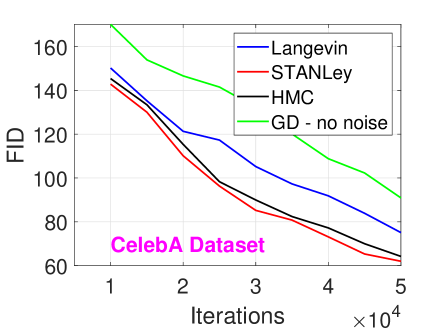
Results. Figure 5 displays the FID curves for all methods. We note that along the iterations, the STANLEY outperforms the other baseline and is similar to HMC, while only requiring first order information for the computation of the stepsize whereas HMC computes second order quantity. Even with second order information, the HMC samples does not lead to a better FID.
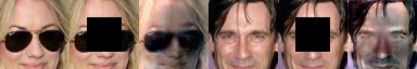

Figure 6 shows the visual check on different samples between our method and its ablated form, i.e., the vanilla Langevin sampler based EBM. In addition to a measurable metrics comparison, visual check provide empirical insights on the effectiveness of adding a curvature-informed stepsize in the sampler of our generative model as in STANLEY.
6 Conclusion
We propose in this paper, an improvement of the so-called MCMC based Energy-Based models. In the particular case of a highly nonlinear structural model of the EBM, more precisely a Convolutional Neural Network in our paper, we tackle the complex task of sampling negative samples from the energy function. The multi-modal and highly curved landscape one must sample from inspire our technique called STANLEY, and based on a Stochastic Gradient Anisotropic Langevin Dynamics, that updates the Markov Chain using an anisotropic stepsize in the vanilla Langevin update. We provide strong theoretical guarantees for our novel method, including uniform ergodicity and geometric convergence rate of the transition kernels to the stationary distribution of the chain. Our method is tested on several benchmarks data and image generation tasks including toy and real datasets.
References
- Allassonniere and Kuhn (2015) Stéphanie Allassonniere and Estelle Kuhn. Convergent stochastic expectation maximization algorithm with efficient sampling in high dimension. application to deformable template model estimation. Computational Statistics & Data Analysis, 91:4–19, 2015.
- An et al. (2021) Dongsheng An, Jianwen Xie, and Ping Li. Learning deep latent variable models by short-run MCMC inference with optimal transport correction. In Proceedings of the IEEE Conference on Computer Vision and Pattern Recognition (CVPR), pages 15415–15424, virtual, 2021.
- Atchadé (2006) Yves F Atchadé. An adaptive version for the metropolis adjusted langevin algorithm with a truncated drift. Methodology and Computing in applied Probability, 8(2):235–254, 2006.
- Bottou et al. (2007) Léon Bottou, Olivier Chapelle, Dennis DeCoste, and Jason Weston, editors. Large-Scale Kernel Machines. The MIT Press, Cambridge, MA, 2007.
- Brosse et al. (2019) Nicolas Brosse, Alain Durmus, Éric Moulines, and Sotirios Sabanis. The tamed unadjusted langevin algorithm. Stochastic Processes and their Applications, 129(10):3638–3663, 2019.
- Cotter et al. (2013) Simon L Cotter, Gareth O Roberts, Andrew M Stuart, and David White. MCMC methods for functions: modifying old algorithms to make them faster. Statistical Science, pages 424–446, 2013.
- de Freitas et al. (2001) Nando de Freitas, Pedro A. d. F. R. Højen-Sørensen, and Stuart Russell. Variational MCMC. In Proceedings of the 17th Conference in Uncertainty in Artificial Intelligence (UAI), pages 120–127, Seattle, WA, 2001.
- Deng et al. (2020) Yuntian Deng, Anton Bakhtin, Myle Ott, Arthur Szlam, and Marc’Aurelio Ranzato. Residual energy-based models for text generation. In Proceedings of the 8th International Conference on Learning Representations (ICLR), Addis Ababa, Ethiopia, 2020.
- Doucet et al. (2000) Arnaud Doucet, Simon Godsill, and Christophe Andrieu. On sequential monte carlo sampling methods for bayesian filtering. Statistics and Computing, 10(3):197–208, 2000.
- Du and Mordatch (2019) Yilun Du and Igor Mordatch. Implicit generation and modeling with energy based models. In Advances in Neural Information Processing Systems (NeurIPS), pages 3603–3613, Vancouver, Canada, 2019.
- Du et al. (2020) Yilun Du, Joshua Meier, Jerry Ma, Rob Fergus, and Alexander Rives. Energy-based models for atomic-resolution protein conformations. In Proceedings of the 8th International Conference on Learning Representations (ICLR), Addis Ababa, Ethiopia, 2020.
- Du et al. (2021) Yilun Du, Shuang Li, Joshua B. Tenenbaum, and Igor Mordatch. Improved contrastive divergence training of energy-based models. In Proceedings of the 38th International Conference on Machine Learning (ICML), pages 2837–2848, Virtual Event, 2021.
- Durmus et al. (2017) Alain Durmus, Gareth O Roberts, Gilles Vilmart, and Konstantinos C Zygalakis. Fast Langevin based algorithm for MCMC in high dimensions. The Annals of Applied Probability, 27(4):2195–2237, 2017.
- Gao et al. (2018) Ruiqi Gao, Yang Lu, Junpei Zhou, Song-Chun Zhu, and Ying Nian Wu. Learning generative convnets via multi-grid modeling and sampling. In Proceedings of the 2018 IEEE Conference on Computer Vision and Pattern Recognition (CVPR), pages 9155–9164, Salt Lake City, UT, 2018.
- Gao et al. (2020) Ruiqi Gao, Erik Nijkamp, Diederik P. Kingma, Zhen Xu, Andrew M. Dai, and Ying Nian Wu. Flow contrastive estimation of energy-based models. In Proceedings of the 2020 IEEE/CVF Conference on Computer Vision and Pattern Recognition (CVPR), pages 7515–7525, Seattle, WA, 2020.
- Girolami and Calderhead (2011) Mark Girolami and Ben Calderhead. Riemann manifold Langevin and Hamiltonian Monte Carlo methods. Journal of the Royal Statistical Society: Series B, 73(2):123–214, 2011.
- Goodfellow et al. (2014) Ian J. Goodfellow, Jean Pouget-Abadie, Mehdi Mirza, Bing Xu, David Warde-Farley, Sherjil Ozair, Aaron C. Courville, and Yoshua Bengio. Generative adversarial nets. In Advances in Neural Information Processing Systems (NIPS), pages 2672–2680, Montreal, Canada, 2014.
- Grenander and Miller (1994) Ulf Grenander and Michael I Miller. Representations of knowledge in complex systems. Journal of the Royal Statistical Society: Series B (Methodological), 56(4):549–581, 1994.
- Gustafsson et al. (2020) Fredrik K. Gustafsson, Martin Danelljan, Goutam Bhat, and Thomas B. Schön. Energy-based models for deep probabilistic regression. In Proceedings of the 16th European Conference on Computer Viosion (ECCV), Part XX, pages 325–343, Glasgow, UK, 2020.
- Gutmann and Hyvärinen (2010) Michael Gutmann and Aapo Hyvärinen. Noise-contrastive estimation: A new estimation principle for unnormalized statistical models. In Proceedings of the Thirteenth International Conference on Artificial Intelligence and Statistics (AISTATS), pages 297–304, Chia Laguna Resort, Sardinia, Italy, 2010.
- Haarnoja et al. (2017) Tuomas Haarnoja, Haoran Tang, Pieter Abbeel, and Sergey Levine. Reinforcement learning with deep energy-based policies. In Proceedings of the 34th International Conference on Machine Learning (ICML), pages 1352–1361, Sydney, Australia, 2017.
- Han et al. (2017) Tian Han, Yang Lu, Song-Chun Zhu, and Ying Nian Wu. Alternating back-propagation for generator network. In Proceedings of the Thirty-First AAAI Conference on Artificial Intelligence (AAAI), pages 1976–1984, San Francisco, CA, 2017.
- Han et al. (2019) Tian Han, Erik Nijkamp, Xiaolin Fang, Mitch Hill, Song-Chun Zhu, and Ying Nian Wu. Divergence triangle for joint training of generator model, energy-based model, and inferential model. In Proceedings of the IEEE Conference on Computer Vision and Pattern Recognition (CVPR), pages 8670–8679, Long Beach, CA, 2019.
- Han et al. (2020) Tian Han, Erik Nijkamp, Linqi Zhou, Bo Pang, Song-Chun Zhu, and Ying Nian Wu. Joint training of variational auto-encoder and latent energy-based model. In Proceedings of the 2020 IEEE/CVF Conference on Computer Vision and Pattern Recognition (CVPR), pages 7975–7984, Seattle, WA, 2020.
- Heusel et al. (2017) Martin Heusel, Hubert Ramsauer, Thomas Unterthiner, Bernhard Nessler, and Sepp Hochreiter. GANs trained by a two time-scale update rule converge to a local nash equilibrium. In Advances in Neural Information Processing Systems (NIPS), pages 6626–6637, Long Beach, CA, 2017.
- Hinton (2002) Geoffrey E. Hinton. Training products of experts by minimizing contrastive divergence. Neural Comput., 14(8):1771–1800, 2002.
- Hyvärinen (2005) Aapo Hyvärinen. Estimation of non-normalized statistical models by score matching. J. Mach. Learn. Res., 6:695–709, 2005.
- Ingraham et al. (2019) John Ingraham, Adam J. Riesselman, Chris Sander, and Debora S. Marks. Learning protein structure with a differentiable simulator. In Proceedings of the 7th International Conference on Learning Representationg (ICLR), New Orleans, LA, 2019.
- Jacob et al. (2020) Pierre E Jacob, John O Leary, and Yves F Atchadé. Unbiased markov chain monte carlo methods with couplings. Journal of the Royal Statistical Society: Series B (Statistical Methodology), 82(3):543–600, 2020.
- Jarner and Hansen (2000) Søren Fiig Jarner and Ernst Hansen. Geometric ergodicity of metropolis algorithms. Stochastic Processes and Their Applications, 85(2):341–361, 2000.
- Jin et al. (2017) Long Jin, Justin Lazarow, and Zhuowen Tu. Introspective classification with convolutional nets. In Advances in Neural Information Processing Systems (NIPS), pages 823–833, Long Beach, CA, 2017.
- Kingma and Ba (2015) Diederik P. Kingma and Jimmy Ba. Adam: A method for stochastic optimization. In Proceedings of the 3rd International Conference on Learning Representations (ICLR), San Diego, CA, 2015.
- Kingma and Welling (2014) Diederik P. Kingma and Max Welling. Auto-encoding variational bayes. In Proceedings of the 2nd International Conference on Learning Representations (ICLR), Banff, Canada, 2014.
- Krizhevsky and Hinton (2009) Alex Krizhevsky and Geoffrey Hinton. Learning multiple layers of features from tiny images. Technical Report, University of Toronto, 2009.
- Lazarow et al. (2017) Justin Lazarow, Long Jin, and Zhuowen Tu. Introspective neural networks for generative modeling. In Proceedings of the IEEE International Conference on Computer Vision (ICCV), pages 2793–2802, Venice, Italy, 2017.
- LeCun et al. (2006) Yann LeCun, Sumit Chopra, Raia Hadsell, M Ranzato, and F Huang. A tutorial on energy-based learning. Predicting Structured Data, 1(0), 2006.
- Lee et al. (2018) Kwonjoon Lee, Weijian Xu, Fan Fan, and Zhuowen Tu. Wasserstein introspective neural networks. In Proceedings of the 2018 IEEE Conference on Computer Vision and Pattern Recognition (CVPR), pages 3702–3711, Salt Lake City, UT, 2018.
- Li et al. (2019) Wenliang Li, Danica J. Sutherland, Heiko Strathmann, and Arthur Gretton. Learning deep kernels for exponential family densities. In Proceedings of the 36th International Conference on Machine Learning (ICML), pages 6737–6746, Long Beach, CA, 2019.
- Liu et al. (2020) Weitang Liu, Xiaoyun Wang, John D. Owens, and Yixuan Li. Energy-based out-of-distribution detection. In Advances in Neural Information Processing Systems (NeurIPS), virtual, 2020.
- Liu et al. (2015) Ziwei Liu, Ping Luo, Xiaogang Wang, and Xiaoou Tang. Deep learning face attributes in the wild. In Proceedings of the 2015 IEEE International Conference on Computer Vision (ICCV), pages 3730–3738, Santiago, Chile, 2015.
- Marshall and Roberts (2012) Tristan Marshall and Gareth O Roberts. An adaptive approach to Langevin MCMC. Statistics and Computing, 22(5), 2012.
- Meyn and Tweedie (2012) Sean P Meyn and Richard L Tweedie. Markov Chains and Stochastic Stability. Springer Science & Business Media, 2012.
- Mikolov et al. (2013) Tomás Mikolov, Ilya Sutskever, Kai Chen, Gregory S. Corrado, and Jeffrey Dean. Distributed representations of words and phrases and their compositionality. In Advances in Neural Information Processing Systems (NIPS), pages 3111–3119, Lake Tahoe, NV, 2013.
- Neal (2011) Radford M Neal. MCMC using hamiltonian dynamics. Handbook of Markov Chain Monte Carlo, 2(11):2, 2011.
- Ngiam et al. (2011) Jiquan Ngiam, Zhenghao Chen, Pang Wei Koh, and Andrew Y. Ng. Learning deep energy models. In Proceedings of the 28th International Conference on Machine Learning (ICML), pages 1105–1112, Bellevue, WA, 2011.
- Nijkamp et al. (2019) Erik Nijkamp, Mitch Hill, Song-Chun Zhu, and Ying Nian Wu. Learning non-convergent non-persistent short-run MCMC toward energy-based model. In Advances in Neural Information Processing Systems (NeurIPS), pages 5233–5243, Vancouver, Canada, 2019.
- Nijkamp et al. (2020) Erik Nijkamp, Mitch Hill, Tian Han, Song-Chun Zhu, and Ying Nian Wu. On the anatomy of MCMC-based maximum likelihood learning of energy-based models. In Proceedings of the Thirty-Fourth AAAI Conference on Artificial Intelligence (AAAI), pages 5272–5280, New York, NY, 2020.
- Nilsback and Zisserman (2008) Maria-Elena Nilsback and Andrew Zisserman. Automated flower classification over a large number of classes. In Proceedings of the Sixth Indian Conference on Computer Vision, Graphics & Image Processing (ICVGIP), pages 722–729, Bhubaneswar, India, 2008.
- Pang et al. (2020) Bo Pang, Tian Han, Erik Nijkamp, Song-Chun Zhu, and Ying Nian Wu. Learning latent space energy-based prior model. In Advances in Neural Information Processing Systems (NeurIPS) 2020, virtual, 2020.
- Qiu et al. (2020) Yixuan Qiu, Lingsong Zhang, and Xiao Wang. Unbiased contrastive divergence algorithm for training energy-based latent variable models. In Proceedings of the 8th International Conference on Learning Representations (ICLR), Addis Ababa, Ethiopia, 2020.
- Robbins and Monro (1951) Herbert Robbins and Sutton Monro. A stochastic approximation method. The Annals of Mathematical Statistics, pages 400–407, 1951.
- Robert et al. (2010) Christian P Robert, George Casella, and George Casella. Introducing Monte Carlo methods with R, volume 18. Springer, 2010.
- Roberts and Rosenthal (1998) Gareth O Roberts and Jeffrey S Rosenthal. Optimal scaling of discrete approximations to Langevin diffusions. Journal of the Royal Statistical Society: Series B (Statistical Methodology), 60(1):255–268, 1998.
- Roberts and Rosenthal (2004) Gareth O Roberts and Jeffrey S Rosenthal. General state space Markov chains and MCMC algorithms. Probability Surveys, 1:20–71, 2004.
- Roberts and Tweedie (1996) Gareth O Roberts and Richard L Tweedie. Exponential convergence of Langevin distributions and their discrete approximations. Bernoulli, pages 341–363, 1996.
- Rue et al. (2009) Håvard Rue, Sara Martino, and Nicolas Chopin. Approximate bayesian inference for latent gaussian models by using integrated nested laplace approximations. Journal of the Royal Statistical Society: Series B (Statistical Methodology), 2009.
- Song et al. (2023) Weinan Song, Yaxuan Zhu, Lei He, Ying Nian Wu, and Jianwen Xie. Progressive energy-based cooperative learning for multi-domain image-to-image translation. arXiv preprint arXiv:2306.14448, 2023.
- Song et al. (2019) Yang Song, Sahaj Garg, Jiaxin Shi, and Stefano Ermon. Sliced score matching: A scalable approach to density and score estimation. In Proceedings of the Thirty-Fifth Conference on Uncertainty in Artificial Intelligence (UAI), pages 574–584, Tel Aviv, Israel, 2019.
- Tieleman (2008) Tijmen Tieleman. Training restricted boltzmann machines using approximations to the likelihood gradient. In Proceedings of the Twenty-Fifth International Conference on Machine Learning (ICML), pages 1064–1071, Helsinki, Finland, 2008.
- Wainwright and Jordan (2008) Martin J. Wainwright and Michael I. Jordan. Graphical models, exponential families, and variational inference. Found. Trends Mach. Learn., 1(1-2):1–305, 2008.
- Welling and Hinton (2002) Max Welling and Geoffrey E. Hinton. A new learning algorithm for mean field boltzmann machines. In Proceedings of the International Conference on Artificial Neural Networks (ICANN), pages 351–357, Madrid, Spain, 2002.
- Welling and Teh (2011) Max Welling and Yee Whye Teh. Bayesian learning via stochastic gradient langevin dynamics. In Proceedings of the 28th International Conference on Machine Learning (ICML), pages 681–688, Bellevue, WA, 2011.
- Wolfinger (1993) Russ Wolfinger. Laplace’s approximation for nonlinear mixed models. Biometrika, 80(4):791–795, 1993.
- Xie et al. (2016) Jianwen Xie, Yang Lu, Song-Chun Zhu, and Ying Nian Wu. A theory of generative ConvNet. In Proceedings of the 33nd International Conference on Machine Learning (ICML), pages 2635–2644, New York City, NY, 2016.
- Xie et al. (2017) Jianwen Xie, Song-Chun Zhu, and Ying Nian Wu. Synthesizing dynamic patterns by spatial-temporal generative convnet. In Proceedings of the IEEE Conference on Computer Vision and Pattern Recognition (CVPR), pages 7093–7101, 2017.
- Xie et al. (2018a) Jianwen Xie, Yang Lu, Ruiqi Gao, and Ying Nian Wu. Cooperative learning of energy-based model and latent variable model via MCMC teaching. In Proceedings of the Thirty-Second AAAI Conference on Artificial Intelligence, (AAAI), pages 4292–4301, New Orleans, LA, 2018a. AAAI Press.
- Xie et al. (2018b) Jianwen Xie, Zilong Zheng, Ruiqi Gao, Wenguan Wang, Song-Chun Zhu, and Ying Nian Wu. Learning descriptor networks for 3D shape synthesis and analysis. In Proceedings of the 2018 IEEE Conference on Computer Vision and Pattern Recognition (CVPR), pages 8629–8638, Salt Lake City, UT, 2018b.
- Xie et al. (2019) Jianwen Xie, Ruiqi Gao, Zilong Zheng, Song-Chun Zhu, and Ying Nian Wu. Learning dynamic generator model by alternating back-propagation through time. In Proceedings of the Thirty-Third AAAI Conference on Artificial Intelligence (AAAI), pages 5498–5507, Honolulu, HI, 2019.
- Xie et al. (2020) Jianwen Xie, Yang Lu, Ruiqi Gao, Song-Chun Zhu, and Ying Nian Wu. Cooperative training of descriptor and generator networks. IEEE Trans. Pattern Anal. Mach. Intell., 42(1):27–45, 2020.
- Xie et al. (2021a) Jianwen Xie, Yifei Xu, Zilong Zheng, Song-Chun Zhu, and Ying Nian Wu. Generative PointNet: Deep energy-based learning on unordered point sets for 3D generation, reconstruction and classification. In Proceedings of the IEEE Conference on Computer Vision and Pattern Recognition (CVPR), pages 14976–14985, virtual, 2021a.
- Xie et al. (2021b) Jianwen Xie, Zilong Zheng, Xiaolin Fang, Song-Chun Zhu, and Ying Nian Wu. Learning cycle-consistent cooperative networks via alternating MCMC teaching for unsupervised cross-domain translation. In Proceedings of the Thirty-Fifth AAAI Conference on Artificial Intelligence (AAAI), pages 10430–10440, Virtual Event, 2021b.
- Xie et al. (2021c) Jianwen Xie, Zilong Zheng, and Ping Li. Learning energy-based model with variational auto-encoder as amortized sampler. In Proceedings of the Thirty-Fifth AAAI Conference on Artificial Intelligence (AAAI), pages 10441–10451, Virtual Event, 2021c.
- Xie et al. (2021d) Jianwen Xie, Song-Chun Zhu, and Ying Nian Wu. Learning energy-based spatial-temporal generative ConvNets for dynamic patterns. IEEE Trans. Pattern Anal. Mach. Intell., 43(2):516–531, 2021d.
- Xie et al. (2022a) Jianwen Xie, Zilong Zheng, Xiaolin Fang, Song-Chun Zhu, and Ying Nian Wu. Cooperative training of fast thinking initializer and slow thinking solver for conditional learning. IEEE Trans. Pattern Anal. Mach. Intell., 44(8):3957–3973, 2022a.
- Xie et al. (2022b) Jianwen Xie, Zilong Zheng, Ruiqi Gao, Wenguan Wang, Song-Chun Zhu, and Ying Nian Wu. Generative VoxelNet: Learning energy-based models for 3D shape synthesis and analysis. IEEE Trans. Pattern Anal. Mach. Intell., 44(5):2468–2484, 2022b.
- Xie et al. (2022c) Jianwen Xie, Yaxuan Zhu, Jun Li, and Ping Li. A tale of two flows: Cooperative learning of langevin flow and normalizing flow toward energy-based model. In Proceedings of the Tenth International Conference on Learning Representations (ICLR), Virtual Event, 2022c.
- Xie et al. (2023) Jianwen Xie, Yaxuan Zhu, Yifei Xu, Dingcheng Li, and Ping Li. A tale of two latent flows: Learning latent space normalizing flow with short-run langevin flow for approximate inference. In Proceedings of the Thirty-Seventh AAAI Conference on Artificial Intelligence (AAAI), pages 10499–10509, Washington, DC, 2023.
- Xu et al. (2022) Yifei Xu, Jianwen Xie, Tianyang Zhao, Chris Baker, Yibiao Zhao, and Ying Nian Wu. Energy-based continuous inverse optimal control. IEEE Trans. Neural Networks Learn. Syst. (Early Access), 2022.
- Yu et al. (2020) Lantao Yu, Yang Song, Jiaming Song, and Stefano Ermon. Training deep energy-based models with f-divergence minimization. In Proceedings of the 37th International Conference on Machine Learning (ICML), pages 10957–10967, Virtual Event, 2020.
- Zhang et al. (2020) Jing Zhang, Jianwen Xie, and Nick Barnes. Learning noise-aware encoder-decoder from noisy labels by alternating back-propagation for saliency detection. In Proceedings of the 16th European Conference on Computer Viosion (ECCV), Part XVII, pages 349–366, Glasgow, UK, 2020.
- Zhang et al. (2021) Jing Zhang, Jianwen Xie, Nick Barnes, and Ping Li. Learning generative vision transformer with energy-based latent space for saliency prediction. In Advances in Neural Information Processing Systems (NeurIPS), pages 15448–15463, virtual, 2021.
- Zhang et al. (2022) Jing Zhang, Jianwen Xie, Zilong Zheng, and Nick Barnes. Energy-based generative cooperative saliency prediction. In Proceedings of the Thirty-Sixth AAAI Conference on Artificial Intelligence (AAAI), pages 3280–3290, Virtual Event, 2022.
- Zhang et al. (2023) Jing Zhang, Jianwen Xie, Nick Barnes, and Ping Li. An energy-based prior for generative saliency. IEEE Trans. Pattern Anal. Mach. Intell., 45(11):13100–13116, 2023.
- Zhao et al. (2021) Yang Zhao, Jianwen Xie, and Ping Li. Learning energy-based generative models via coarse-to-fine expanding and sampling. In Proceedings of the 9th International Conference on Learning Representations (ICLR), Virtual Event, 2021.
- Zhao et al. (2023) Yang Zhao, Jianwen Xie, and Ping Li. CoopInit: Initializing generative adversarial networks via cooperative learning. In Proceedings of the Thirty-Seventh AAAI Conference on Artificial Intelligence (AAAI), pages 11345–11353, Washington, DC, 2023.
- Zheng et al. (2021) Zilong Zheng, Jianwen Xie, and Ping Li. Patchwise generative ConvNet: Training energy-based models from a single natural image for internal learning. In Proceedings of the IEEE Conference on Computer Vision and Pattern Recognition (CVPR), pages 2961–2970, virtual, 2021.
- Zhu et al. (1998) Song Chun Zhu, Ying Nian Wu, and David Mumford. Filters, random fields and maximum entropy (FRAME): towards a unified theory for texture modeling. Int. J. Comput. Vis., 27(2):107–126, 1998.
- Zhu et al. (2023) Yaxuan Zhu, Jianwen Xie, and Ping Li. Likelihood-based generative radiance field with latent space energy-based model for 3D-aware disentangled image representation. In Proceedings of the International Conference on Artificial Intelligence and Statistics (AISTATS), pages 4164–4180, Palau de Congressos, Valencia, Spain, 2023.
Appendix A Appendix: Proofs of the Theoretical Results
A.1 Sketch of the Proof of Theorem 4.2
Notations for the proof: We denote by , the pdf of the Gaussian proposal of Line 3 for any current state of the chain and dependent on the EBM model parameter . The transition kernel from to is denoted by . is a subset of and is a Borel set of .
The proof of our results are divided into two main parts. We first prove the existence of a small set for our transition kernel , noted showing that for any state, the Markov Chain moves away from it. It constitutes the first step toward proving its irreducibility and aperiodicity. Then, we will establish the so-called drift condition, also known as the Foster-Lyapunov condition, crucial to proving the convergence of the chain. The drift condition ensures the recurrence of the chain as the property that a chain returns to its initial state within finite time, see Roberts and Rosenthal (1998, 2004) for more details. Uniform ergodicity is then established as a consequence of those drift conditions and thus proving (9).
(i) Existence of a small set: Let be a compact subset of the state space . We recall the definition of the transition kernel in the case of a Metropolis adjustment and for any model parameter and state :
where we have defined the Metropolis ratio between two states as . Under H1 and due to the fact that the threshold th leads to a symmetric positive definite covariance matrix with bounded non zero eigenvalues, then the following holds:
| (11) |
for all and where and are the corresponding standard deviations of the two Gaussian distributions and . We denote by the ratio and define the quantity
| (12) |
where we have used assumptions H1 and H2. Then,
According to (12), we can find a compact set such that where where Z is the normalizing constant of the pdf and the proposal distribution is bounded from below by some quantity noted . The calculations above prove (8), i.e., the existence of a small set for our family of transition kernels .
(ii) Drift condition and ergodicity: We begin by proving that satisfies a drift property. For a given EBM parameter , we can see in Jarner and Hansen (2000) that the drift condition boils down to proving that
where is the drift function defined in (6) Let denote the acceptation set, i.e., by
| (13) |
for any state and its complementary set . The remaining of the proof is composed of three main steps. Step (1) shows that for any ,
where the smoothness of a Gaussian pdf, assumption H1 and a collection of inequalities based on (13), its complentary set and the interval in (11). Then, using an important intermediary result, stated in Lemma A.1, that initiates a relation between the set of accepted states noted and the cone designed so that it does not depend on the model parameter .
Define and . Then for , .
Noting the limit inferior as , Step (2) establishes that where is a constant, independent of all the other quantities towards showing uniformity of the final result. Finally, Step (3) uses the inequality dependent of and defines the V function, independent of , as in order to establish the main result of Theorem 4.2, i.e.,
Setting , and proves the uniformity of the inequality (9).
The complete proof is deferred in the appendix and is also developed in Allassonniere and Kuhn (2015) in the context of Bayesian Mixed Effect models trained with the EM algorithm.
A.2 Proof of Theorem 4.2
Theorem.
Proof.
Notations used throughout the proof are listed in Table 1
| Transition kernel of the MCMC defined by (5) | ||
| Subset of and small set for kernel | ||
| Ball around of radius | ||
| Acceptance set at state such that | ||
| Complementary set of | ||
| Probability density function of the Gaussian proposal | ||
| Stationary/Target distribution under model | ||
| Transition kernel from state to state | ||
| Pdf of a centered Normal distribution of standard deviation |
The proof of our results are divided into two parts. We first prove the existence of a set noted as a small set for our family of transition kernels . Proving a small set is crucial in order to show that for any state, the Markov Chain does not stay in the same state, and thus help in proving its irreducibility and aperiodicity.
Then, we will prove the drift condition towards a small set. This condition is crucial to prove the convergence of the chain since it states that the kernels tend to attract elements into that set. finally, uniform ergodicity is established as a consequence of those drift conditions.
(i) Existence of small set: Let be a compact subset of the state space . We also denote the probability density function (pdf) of the Gaussian proposal of Line 3 as for any current state of the chain and dependent on the EBM model parameter . Given STANLEY’s MCMC update, at iteration , the proposal is a Gaussian distribution of mean and covariance .
We recall the definition of the transition kernel in the case of a Metropolis adjustment and for any model parameter and state :
| (16) |
where we have defined the Metropolis ratio between two states and as . Thanks to Assumption H1 and due to the fact that the threshold th leads to a symmetric positive definite covariance matrix with bounded non zero eigenvalues implies that the proposal distribution can be bounded by two zero-mean Gaussian distributions as follows:
| (17) |
where and are the corresponding standard deviation of the distributions and and are some scaling factors.
We denote by the ratio and given the assumptions H1 and H2, define the quantity
| (18) |
Likewise, the proposal distribution is bounded from below by some quantity noted . Then,
| (19) |
Then, given the definition of (18), we can find a compact set such that where where Z is the normalizing constant of the pdf . The calculations above prove (8), i.e., the existence of a small set for our family of transition kernels .
(ii) Drift condition and ergodicity: We first need to prove the fact that our family of transition kernels satisfies a drift property.
For a given EBM model parameter , we can see in Jarner and Hansen (2000) that the drift condition boils down to proving that for the drift function noted and defined in (6), we have
| (20) |
Throughout the proof, the model parameter is set to an arbitrary . Let denote the acceptation set, i.e., by for any state and its complementary set .
Step (1): Following our definition of the drift function in (6) we obtain:
| (21) | ||||
| (22) |
where (a) is due to (6).
Furthermore, according to (17), we thus have that, for any state in the acceptance set :
| (23) |
For any state in the complementary set of the acceptance set, noted , we also have the following:
| (24) |
While we can define the level set of the stationary distribution as for some state , a neighborhood of that level set is defined as . H1 ensures the existence of a radial such that for all , then with . Since the function is smooth, it is known that there exists a constant such that for , we have that
| (25) |
for some small enough and where denotes the ball around of radius . Then combining (23) and (25) we have that:
| (26) |
Conversely, we can define the following set where if and . Then using the second part of H1, there exists a radius , such that for with we have
| (27) |
where . Note that H1 implies that when . Likewise with we have
| (28) |
Same arguments can be obtained for the second term of (21), i.e., and we obtain, plugging the above in (21) that:
| (29) |
Since is the complementary set of , the above inequality yields
| (30) |
Step (2): The final step of our proof consists in proving that where is a constant, independent of all the other quantities.
Given that the proposal distribution is a Gaussian and using assumption H1 we have the existence of a constant depending on as defined above (the radius of the ball ) such that
| (31) |
Then for any , we obtain that . A particular subset of used throughout the rest of the proof is the cone defined as
| (32) |
Using Lemma A.1, we have that . Then, we observe that
| (33) |
where we have used (17) in (a) and applied Lemma A.1 in (b).
If we define the translation of vector by the operator , then
| (34) |
Recalling the objective of Step (2) that is to find a constant such that , we deduce from (34) that since the set does not depend on the EBM model parameter and that once translated by the resulting set is independent of (but depends on , see definition (32), then the integral in (34) is independent of thus concluding on the existence of the constant such that
Thus proving the second part of (20) which is the main drift condition we ought to demonstrate. The first part of (20) can be proved by observing that is smooth on according to H2 and by construction of the transition kernel. Smoothness implies boundedness on the compact .
Step (3): We now use the main proven equations in (20) to derive the second result (9) of Theorem 4.2.
We will begin by showing a similar inequality for the drift function , thus not having uniformity, as an intermediary step. The Drift property is a consequence of Step (2) and (34) shown above. Thus, there exists , such that for all :
| (35) |
where is defined by (6). Using the two functions defined in (7), we define for , the function independent of as follows:
| (36) |
where , is defined in H3 and is defined in (6). Thus for , and :
| (37) |
where we have used the Young’s inequality in (a) and the definition of , see (7), in (b). Then plugging (35) in (37), we have
| (38) | ||||
| (39) | ||||
| (40) | ||||
| (41) | ||||
| (42) |
A.3 Proof of Lemma A.1
Lemma.
Define and . Then for , .
Proof.
In order to show the inclusion of the set in we start by selecting the quantity for and where is the radius of the ball used in (25) such that . We will now show that .
By the generalization of Rolle’s theorem applied on the stationary distribution , we guarantee the existence of some such that:
| (43) |
Expanding yields:
| (44) |
Yet, under assumption H1, there exists such that
and for any we note that , by construction of the set. Thus,
| (45) |
where is used in the definition of . Additionally we let denote the vector multiplication between the normalized gradient and . Then plugging (45) into (44) leads to and implies, using (31), that . Finally implies that , concluding the proof of Lemma A.1.
∎