Gradient Descent Fails to Learn High-frequency Functions and Modular Arithmetic

Abstract

Classes of target functions containing a large number of approximately orthogonal elements are known to be hard to learn by the Statistical Query algorithms. Recently this classical fact re-emerged in a theory of gradient-based optimization of neural networks. In the novel framework, the hardness of a class is usually quantified by the variance of the gradient with respect to a random choice of a target function.

A set of functions of the form $x\to ax\bmod p$, where $a$ is taken from ${\mathbb{Z}}_{p}$, has attracted some attention from deep learning theorists and cryptographers recently. This class can be understood as a subset of $p$-periodic functions on ${\mathbb{Z}}$ and is tightly connected with a class of high-frequency periodic functions on the real line.

We present a mathematical analysis of limitations and challenges associated with using gradient-based learning techniques to train a high-frequency periodic function or modular multiplication from examples. We highlight that the variance of the gradient is negligibly small in both cases when either a frequency or the prime base $p$ is large. This in turn prevents such a learning algorithm from being successful.

Keywords modular multiplication $\cdot$ high-frequency periodic functions $\cdot$ hardness of learning $\cdot$ gradient-based optimization $\cdot$ barren plateau $\cdot$ statistical query

1 Introduction

Gradient-based optimization is behind the success of modern deep learning methods. Therefore, the study of its limitations is a central theoretical and experimental topic. Already early studies on the subject recognized the vanishing gradient problem as a key reason for the failure to learn high-quality models. Today it is clear that gradient vanishing can be caused by problems with an architecture of a neural network (which inspired many remedies such as LSTM [1], residual networks [2, 3], using ReLU as an activation function, etc.), as well as by an implicit hardness of a class of target functions [4, 5, 6, 7] (or, a combination of reasons).

Recently, a useful relationship was established between gradient-based methods and the so-called Statistical Query (SQ) model [8, 9]. This led to an understanding that classes of target functions with a large statistical query dimension are unlikely to be trainable by modern gradient-based algorithms such as SGD, Adam, Nesterov, etc. In a practical setting, this reveals itself in a vanishing gradient problem, when for many iterations of an algorithm an objective function fluctuates around a certain value (or, easily overfits). This type of behavior is sometimes called the barren plateau phenomenon.

Mathematically, the barren plateau phenomenon can be described in terms of a high concentration of the gradient around its mean (or, equivalently, a negligibly small variance) when a target function is sampled (usually, uniformly) from a hypothesis space. This demonstrates that the information content of the gradient about a key parameter of the target function is, in fact, very small. A classical example of a hypothesis space for which this variance is provably small is a set of parity functions [10]. Other examples with obtained upper bounds on the variance of the gradient with respect to a hypothesis set include parameterized quantum circuit training [11] and tensor network training [12] problems. For the current paper, a key example was analyzed by [13], who considered a set of functions $\{\psi({\mathbf{w}}^{\top}{\mathbf{x}})\mid{\mathbf{w}}\in{\mathbb{R}}^{d},\|{\mathbf{w}}\|=r\}$, where $\psi$ is 1-periodic, both the dimension $d$ and the norm $r$ grow moderately, and proved that the variance is bounded by $\mathcal{O}\big{(}{\rm exp}(-\Theta(d))+{\rm exp}(-\Theta(r))\big{)}$.

The problem of training basic modular arithmetical operations from data also attracted some attention, though that problem seemingly belongs to a different context. First, it was noticed that the multiplication (or, the division) modulo some prime number $p$ is a mapping that is hard to train even for small primes (e.g. $p=97$) [14, 15]. The training process itself has an atypical structure — first, an SGD algorithm fluctuates around a certain mean value (or, even overfits), and then abruptly falls into a good minimum. The grokking is a term that was coined for this type of training process. The time until the second regime starts strongly depends on the initial value (whether it is close enough to the so-called “Goldilocks” zone) and for larger primes the second regime does not occur at all. In this line of research, an interest in training modular multiplication is mainly defined by the role the task plays in the demonstration of different aspects of grokking such as, for example, the so-called “LU mechanism”. Though grokking was reported in more real-world datasets from computer vision, natural language processing and molecule property prediction [16], training modular multiplication is still viewed as an archetypical case of the phenomenon.

Training the modular arithmetic operations has found applications in neural cryptanalysis. In such applications, one of the multipliers in modular multiplication is sometimes fixed (and called a secret). In [17], for the needs of lattice cryptography, experiments on training the modular multiplication were extended to include the dot product in ${\mathbb{Z}}_{p}^{n}$. To be specific, the mentioned paper studied the learnability of the mapping $f:{\mathbb{Z}}_{p}^{n}\to{\mathbb{Z}}_{p}$, $f(x_{1},\cdots,x_{n})=a_{1}x_{1}+\cdots+a_{n}x_{n}\bmod p$ from a set of examples $\{({\mathbf{y}}_{i},f({\mathbf{y}}_{i}))\mid{\mathbf{y}}_{i}\in{\mathbb{Z}}_{p}^{n},1\leq i\leq N\}$ where $(a_{1},\cdots,a_{n})$ was uniformly sampled from ${\mathbb{Z}}_{p}^{n}$.

In our paper, we are interested in the case $n=1$ only (though our results can be easily generalized to arbitrary $n$). Given some prime number $p>2$, a basic approach of our paper is to view the mapping $x\to ax\bmod p$ as a $p$-periodic function on a ring of integers ${\mathbb{Z}}$. Periodic functions on ${\mathbb{Z}}$ are analogous to periodic functions on ${\mathbb{R}}$, therefore we study these two kinds of target functions together using similar techniques. Thus, we also study the learnability of the function $f:{\mathbb{R}}\to{\mathbb{R}},f(x)=\psi(ax)$, where $\psi$ is 1-periodic and $a$ is sampled uniformly from the set $\{0,\cdots,A-1\}$. In both cases, our proofs are based on the adaptation of the proof technique for orthogonal functions from [10]. We emphasize that their result is not directly applicable to the class of functions that we consider in this paper (high-frequency one-dimensional waves or output bits of the modular multiplication) since these functions are not orthogonal with respect to a uniform distribution over the domain. However, they are approximately pairwise orthogonal, and the proof of this fact is the core of our work.

In both cases, we prove the existence of the barren plateau phenomenon, when either $p$ is a large prime (e.g. a typical prime base in cryptography), or $A$ is large in the second case. Our paper is organized in the following way. In Section 2 we give an overview of obtained results. Section 3 is dedicated to empirical verification of our main claims. Due to its technical simplicity, we first give a bound on the variance of the gradient w.r.t. a hypothesis set of periodic functions on the real line (Section 4). Then, in Section 5 we give a more elaborate proof of a bound on the variance of the gradient w.r.t. hypothesis sets $\{x\to ax\bmod p\}_{a\in{\mathbb{Z}}_{p}^{\ast}}$ and $\{x\to[ax\bmod p]_{r}\}_{a\in{\mathbb{Z}}_{p}^{\ast}}$ where $[x]_{r}$ is the $r$th bit from the end in a binary representation of $x$. Our proof technique is based on bounding the r.h.s. of the Boas-Bellman inequality [18, 19]. To establish the connection with the SQ model, in Section 7 we show that any upper bound on the latter expression directly leads to a lower bound on the so-called SQ dimension of a hypothesis set. Thus, all our bounds can be also turned to lower bounds on the SQ dimension. This implies that high-frequency functions on the real line and modular multiplication are hard not only for gradient-based methods but also for any SQ algorithm.

1.1 Notation

Bold-faced lowercase letters ($\mathbf{x}$) denote vectors, bold-faced uppercase letters ($\mathbf{A}$) denote matrices. Regular lowercase letters ($x$) denote scalars (or set elements), and regular uppercase letters ($X$) denote random variables (or random elements). $\|\cdot\|$ denotes the Euclidean norm: $\|\mathbf{x}\|:=\sqrt{\mathbf{x}^{\top}\mathbf{x}}$. For $\mathbf{x}\in\mathbb{C}^{n}$, conjugate transpose is denoted by $\mathbf{x}^{\dagger}$. For any finite set or interval $\mathcal{S}$, sampling $X$ uniformly from $\mathcal{S}$ is denoted by $X\sim\mathcal{S}$.

Given $f:\,\mathbb{N}\to\mathbb{R}$ and $g:\,\mathbb{N}\to\mathbb{R}_{+}$, we write $f\ll g$ if there exist universal constants $\alpha,\beta\in\mathbb{R}_{+}$ such that for all natural numbers $x>\beta$ we have $|f(x)|\leq\alpha g(x)$. When $f,g:\mathbb{N}\to\mathbb{R}_{+}$, we write $f\asymp g$ if $f\ll g$ and $g\ll f$. If $n\in{\mathbb{R}}$ is such that $f(x)\ll g(x)|\log^{n}g(x)|$ then we simply write $f(x)=\tilde{\mathcal{O}}(g(x))$. If we have $f(x)=\tilde{\mathcal{O}}(g(x))$ and $g(x)=\tilde{\mathcal{O}}(f(x))$, then we write $f(x)=\tilde{\Theta}(g(x))$.

$\mathbb{Z}_{p}$ is the set $\{0,1,\ldots,p-1\}$, equipped with two operations, which work as usual addition and multiplication, except that the results are reduced modulo $p$. $\mathbb{Z}_{p}^{\ast}$ denotes the set of elements in $\mathbb{Z}_{p}$ that are relatively prime to $p$. We are mainly interested in the case when $p$ is a prime number greater than 2. In this case $\mathbb{Z}_{p}^{\ast}=\{1,\ldots,p-1\}$. By abuse of notation, we sometimes treat elements of $\mathbb{Z}_{p}$ (and of $\mathbb{Z}_{p}^{\ast}$) as integers in $\mathbb{Z}$. Given two positive integers $a$ and $p$, $a\bmod p$ is the remainder of the Euclidean division of $a$ by $p$, where $a$ is the dividend and $p$ is the divisor. For $a,b\in{\mathbb{Z}}$, we denote ordinary multiplication simply by $ab$ and $ab\bmod p$ by $a\cdot b$ (the base $p$ is always clear from the context). If $a^{-1}$ is an inverse of $a\in{\mathbb{Z}}_{p}^{\ast}$ in the multiplicative group $({\mathbb{Z}}_{p}^{\ast},\cdot)$, then $b\cdot a^{-1}$ is denoted by $b/a$. Also, below $[\cdot]$ denotes the Iverson bracket, i.e. $[{\rm True}]=1$, $[{\rm False}]=0$.

2 Main results

Let $\psi:{\mathbb{R}}\to{\mathbb{R}}$ be a 1-periodic function on the real line that has a bounded variation. The latter condition captures all piecewise Lipschitz functions. Such a function induces a family of one-dimensional waves

$$h_{a}(x)=\psi(ax),$$ (1)

parametererized by the frequency $a\in\{0,\cdots,A-1\}$ where $A$ is a large integer. Let us denote $\mathcal{H}_{A}=\{h_{a}\}_{a\in{\mathbb{Z}}_{A}}$.

Consider the following supervised learning task. Let us assume that $a$ was generated uniformly from the set $\{0,\cdots,A-1\}$ and our goal is to approximate $h_{a}(x)$ in terms of $L_{2}([0,1])$-metrics. That is, we solve the task

$$\min\limits_{{\mathbf{w}}\in\mathcal{O}}\|h_{a}(x)-p({\mathbf{w}},x)\|^{2}_{L_{2}([0,1])}$$ (2)

where $p({\mathbf{w}},x)$ is some family of functions, parameterized by the weight ${\mathbf{w}}\in\mathcal{O}\subseteq{\mathbb{R}}^{s}$, e.g. given as a neural network.

For the task (2) to be solvable by some gradient-based method (e.g., SGD, Nesterov, Adam), the gradient of the objective function at a given point ${\mathbf{w}}$ should have enough mutual information with the random variable $a$. Following [13], we measure the information content of the gradient about $a$ by

$${\rm Var}_{a\sim{\mathbb{Z}}_{A}}\big{[}\nabla_{\mathbf{w}}\|h_{a}(x)-p({\mathbf{w}},x)\|^{2}_{L_{2}([0,1])}\big{]},$$ (3)

which is called the variance of the gradient w.r.t. to the hypothesis space $\mathcal{H}_{A}$ and is denoted by ${\rm Var}(\mathcal{H}_{A},{\mathbf{w}})$. The smaller ${\rm Var}(\mathcal{H}_{A},{\mathbf{w}})$ is the smaller the information content of the gradient.

Our key bound reads as

$${\rm Var}(\mathcal{H}_{A},{\mathbf{w}})=\tilde{\mathcal{O}}(\frac{1}{\sqrt{A}}),$$ (4)

where $\tilde{\mathcal{O}}$ hides a factor that depends polynomially on the logarithm of $A$ and factors that are bounded by derivatives of the neural network w.r.t. its weights and the variation of $\psi$. The equation (4) demonstrates that the gradient becomes non-informative as the highest frequency $A$ grows. Our proof is given in Section 4 and it is based on a certain combination of the Boas-Bellman inequality with some standard bounds (namely, the Erdős-Turán-Koksma inequality) from the ergodic theory of translations on a two-dimensional torus.

Remark 1.

The learnability by gradient-based methods of the hypothesis space

$$\mathcal{H}_{r}=\{h_{{\mathbf{w}}}:{\mathbb{R}}^{d}\to{\mathbb{R}}\mid\|{\mathbf{w}}\|=r,h_{{\mathbf{w}}}({\mathbf{x}})=\psi({\mathbf{w}}^{T}{\mathbf{x}})\}$$

was a subject in [13], who showed ${\rm Var}(\mathcal{H}_{r},w)=\mathcal{O}({\rm exp}(-\Theta(d))+{\rm exp}(-\Theta(r)))$. This result implies the failure of gradient-based learning when both $d$ and $r$ grow moderately. Our bound shows that the phenomenon of poor learnability of waves maintains in the smallest possible dimension ($d=1$) under the condition that the frequency grows exponentially.

We proceed to study the observed phenomenon and consider a discrete version of high-frequency waves, now on ${\mathbb{Z}}$ (not ${\mathbb{R}}$). Now, let $\psi:{\mathbb{Z}}\to{\mathbb{R}}$ be a $p$-periodic function on a ring of integers, i.e. $\psi(x+p)=\psi(x)$, where $p>2$ is prime. Let us introduce the hypothesis

$$\tilde{h}_{a}:{\mathbb{Z}}\to{\mathbb{R}},\tilde{h}_{a}(x)=\psi(ax)$$ (5)

parametererized by the frequency $a\in{\mathbb{Z}}^{\ast}_{p}$. Let us denote $\tilde{\mathcal{H}}_{p}=\{\tilde{h}_{a}\}_{a\in{\mathbb{Z}}^{\ast}_{p}}$. Note that any function from $\tilde{\mathcal{H}}_{p}$ is defined by its restriction on the set ${\mathbb{Z}}_{p}$, therefore, we alternatively can study the hypothesis set $\mathring{\mathcal{H}}_{p}=\{\mathring{h}_{a}:{\mathbb{Z}}_{p}\to{\mathbb{R}}\mid\mathring{h}_{a}(x)=t(a\cdot x),a\in{\mathbb{Z}}_{p}^{\ast}\}$ where $t$ is a restriction of $\psi$ on ${\mathbb{Z}}_{p}$.

Our interest towards the hypothesis set $\mathring{\mathcal{H}}_{p}$ is motivated by specific cases when (a) $t(x)=\frac{(a\cdot x)-\frac{p}{2}}{\sqrt{\frac{p^{2}}{12}-\frac{p}{6}}}[x\neq 0]$ or (b) $t(x)=[x]_{r}$ where $[x]_{r}$ is the $r$th bit from the end in a binary representation of $x$. The case (a) corresponds to the standardized hypothesis set $\{x\to a\cdot x\}_{a\in{\mathbb{Z}}_{p}^{\ast}}$ and the case (b) to the set $\{x\to[a\cdot x]_{r}\}_{a\in{\mathbb{Z}}_{p}^{\ast}}$. Let us define the variance w.r.t. $\mathring{\mathcal{H}}_{p}$ by

$${\rm Var}(\mathring{\mathcal{H}}_{p},{\mathbf{w}})={\rm Var}_{a\sim{\mathbb{Z}}^{\ast}_{p}}\big{[}\nabla_{\mathbf{w}}{\mathbb{E}}_{x\sim{\mathbb{Z}}^{\ast}_{p}}[L(\mathring{h}_{a}(x),p({\mathbf{w}},x))]\big{]},$$ (6)

where $L$ is a square loss function for the case (a) and $L(y,y^{\prime})=l(yy^{\prime})$, where $l$ is some 1-Lipschitz function, for the case (b).

In Sections 5 and 6 we prove that in both cases we have

$${\rm Var}(\mathring{\mathcal{H}}_{p},{\mathbf{w}})=\tilde{\mathcal{O}}(\frac{1}{\sqrt{p}}),$$ (7)

where, again, $\tilde{\mathcal{O}}$ hides factors that depend polynomially on the logarithm of $p$ and on derivatives of our model $p({\mathbf{w}},x)$ w.r.t. its weights (Theorems 15 and 16).

Remark 2.

From the first site, a proof of the bound (7) is substantially different from the proof of (4). In fact, there is an analogy between the two. Both proofs are based on the application of the Boas-Bellman inequality. When we prove (7), we first obtain a general bound on ${\rm Var}(\mathring{\mathcal{H}}_{p},{\mathbf{w}})$ in terms of properties of the Discrete Fourier Transform of $t$, and then apply the general bound to the cases (a) and (b) of modular multiplication. As was already mentioned, a proof of (4) is based on the Erdős-Turán-Koksma inequality, i.e. on the statement whose canonical proof is itself based on Fourier analysis. We believe that both bounds are edges of a more general theory (which, probably, can be formulated for periodic functions on general abelian groups), but this falls out of the scope of our paper.

Remark 3.

From our bounds on the variances, using Theorem 10 of [13], one can derive the following statement: an output of any algorithm with access to an approximate gradient oracle can distinguish between different values of the parameter $a$ of the target function $h_{a}$ (or, of $\mathring{h}_{a}$) only if the number of its iterations is substantially greater than $\tilde{\Theta}(A^{1/6})$ (or, $\tilde{\Theta}(p^{1/6})$). This statement implies that for large $A$ (or $p$), a gradient-based method fails for the task of training the set of targets $\mathcal{H}_{A}$ (or $\mathring{\mathcal{H}}_{p}$) if the hypothesis $h_{a}$ (or, $\mathring{h}_{a}$) depends on the parameter $a$ in a highly sensitive way (which is usually the case). In the last section of the paper we also obtain lower bounds on the statistical query dimension of our classes, and they grow at least as $\tilde{\Theta}(A^{1/3})$ (or, $\tilde{\Theta}(p^{1/3})$).

3 Empirical Verification

Failure to learn high-frequency waves on ${\mathbb{R}}$.

We verified the hardness of the task (2) for the stochastic gradient descent algorithm directly by minimizing the MSE loss that approximates the square of the $L_{2}([0,1])$-distance. We chose $\psi(x)=\{x\}$ where $\{x\}$ is the fractional part of $x\in{\mathbb{R}}$. For a large $a\in{\mathbb{N}}$ and a random $X\sim[0,1]$, $h_{a}(X)=\psi(aX)$ is distributed approximately uniformly on $[0,1]$. If we consider the mean of the uniform distribution on $[0,1]$ as a baseline approximation of $h_{a}(x)$, then the corresponding squared $L_{2}([0,1])$-distance of such an approximation equals the variance of this distribution, i.e. $\frac{1}{12}$. As Figure 1 shows, our model (a 3-layer neural network with dimensions of layers $[1,64,128,1]$ and the ReLU activation function) is unable to achieve the MSE loss smaller than the trivial $\frac{1}{12}$.

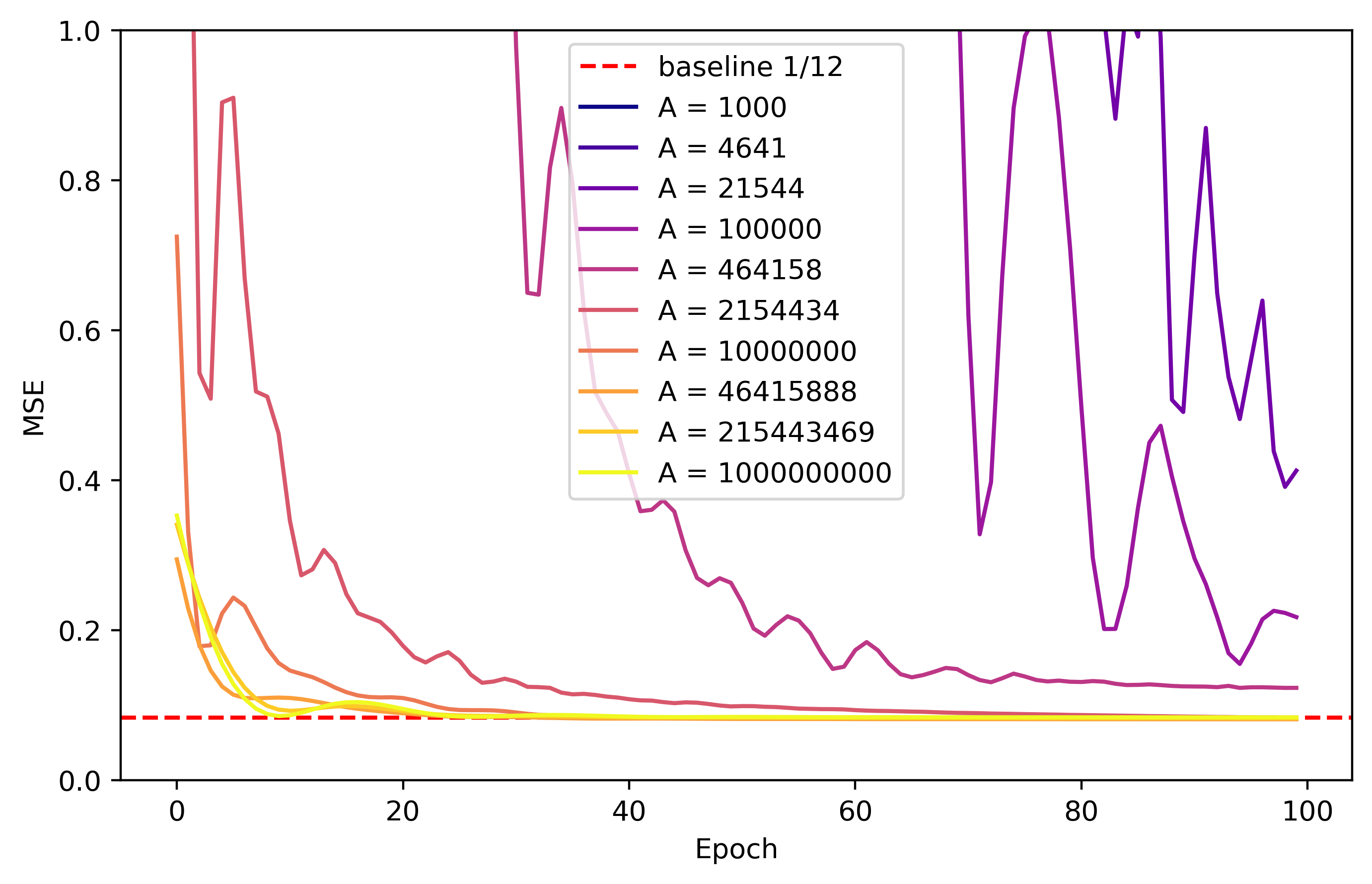
Figure 1: Learning the high-frequency wave on ${\mathbb{R}}$ with a 3-layer dense network with ReLU activation. For each $A$, the coefficient $a$ was sampled randomly 10 times from ${\mathbb{Z}}_{A}$, and an average MSE loss as a function of an epoch is depicted. The horizontal asymptote corresponds to ${\rm MSE}=\frac{1}{12}$.

Concentration of the Gradient.

Let us verify empirically the statement (7) for the last bit of modular multiplication. Let $p(\mathbf{w},x)$ be a neural network that we may want to train to learn the mapping $x\mapsto(-1)^{a\cdot x}$, $x\in\mathbb{Z}_{p}^{\ast}$, where $\mathbf{w}\in\mathbb{R}^{s}$ are all parameters of the neural network. Since $(-1)^{a\cdot x}=(-1)^{[a\cdot x]_{1}}$, this mapping computes the last bit of modular multiplication $a\cdot x$. Let $\nabla L_{a}(\mathbf{w})$ be the gradient of the binary cross-entropy loss function at $\mathbf{w}$. We sample $\mathbf{w}_{1},\ldots,\mathbf{w}_{20}$ from $\mathbb{R}^{s}$ using the default PyTorch initializer, and for each $\mathbf{w}_{i}$, we compute

$$v(\mathbf{w}_{i}) =\operatorname*{\mathbb{E}}_{A\sim\mathbb{Z}_{p}^{\ast}}\left\|\nabla L_{A}(\mathbf{w}_{i})-\operatorname*{\mathbb{E}}_{A^{\prime}\sim\mathbb{Z}_{p}^{\ast}}\nabla L_{A^{\prime}}(\mathbf{w}_{i})\right\|^{2},$$ (8)

$$g(\mathbf{w}_{i}) =\operatorname*{\mathbb{E}}_{X\sim\mathbb{Z}_{p}^{\ast}}\left\|\frac{\partial}{\partial\mathbf{w}}p_{\mathbf{w}}({X})\right\|^{2}.$$ (9)

According to Theorem 16, the values $\frac{v(\mathbf{w}_{i})}{g(\mathbf{w}_{i})}$ should be of order $\tilde{\mathcal{O}}\left(\frac{1}{\sqrt{p}}\right)$. Thus, we plot $\operatorname*{\mathbb{E}}_{i\sim\{1,\ldots,20\}}\left[\frac{v(\mathbf{w}_{i})}{g(\mathbf{w}_{i})}\cdot\sqrt{p}\right]$ against $p$ in Figure 3.

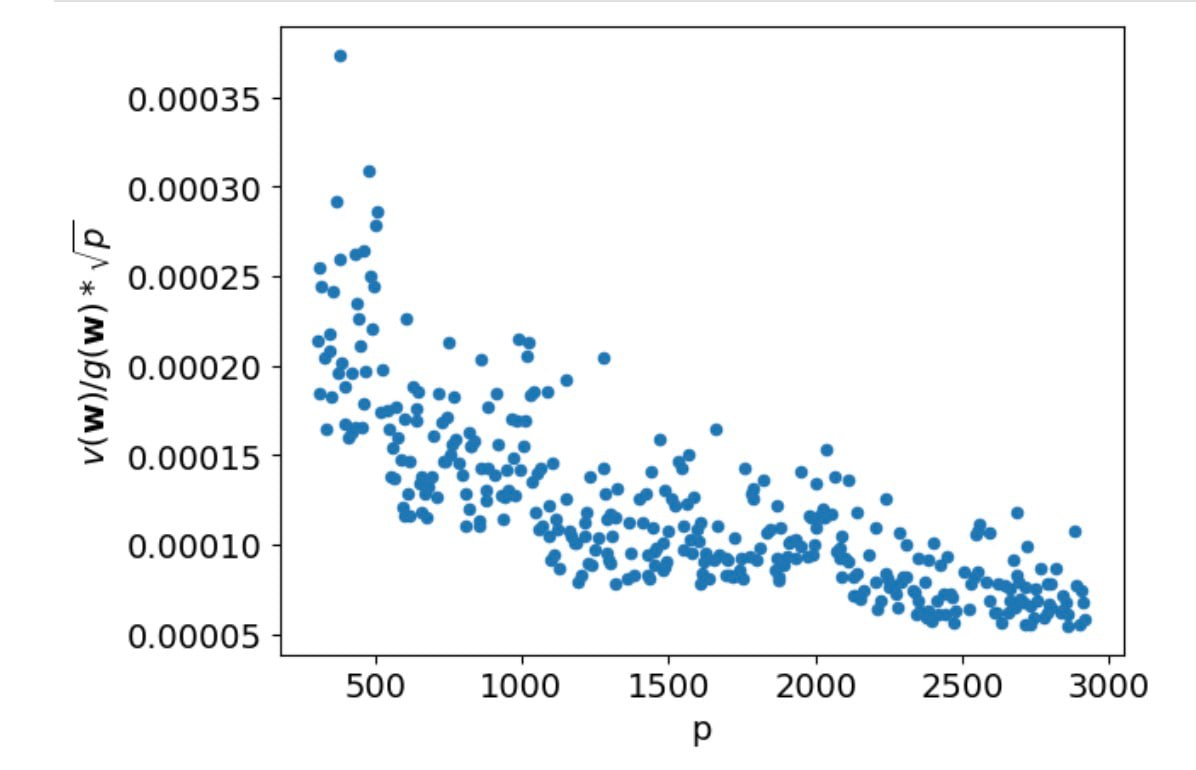
Figure 2: Verifying the statement of Theorem 16. For prime numbers $p$ in $[300,3000]$, we plot the left-hand side of (7) divided by the average squared norm of the neural network’s gradient (9) and multiplied by $\sqrt{p}$. The resulting curve is of order $\tilde{\mathcal{O}}(1)$. Moreover, it even decreases.

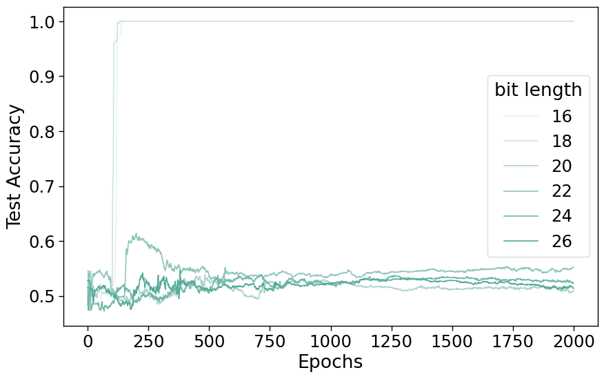
Figure 3: Learning the parity bit of multiplication modulo $p$ with a 3-layer width-1000 dense network. Darker shades correspond to longer bit lengths. For each bitlength $n$, $p$ is chosen randomly from the prime numbers in the interval $[2^{n-1},2^{n}-1]$.

As we can see, this expression is bounded as $p$ grows, which confirms the statement of the theorem. In fact, Figure 4 suggests that our upperbound (7) can be improved, i.e. the variance of the gradient decays like $\tilde{\mathcal{O}}(\frac{1}{p})$, not like $\tilde{\mathcal{O}}(\frac{1}{\sqrt{p}})$ (at a random point ${\mathbf{w}}$).

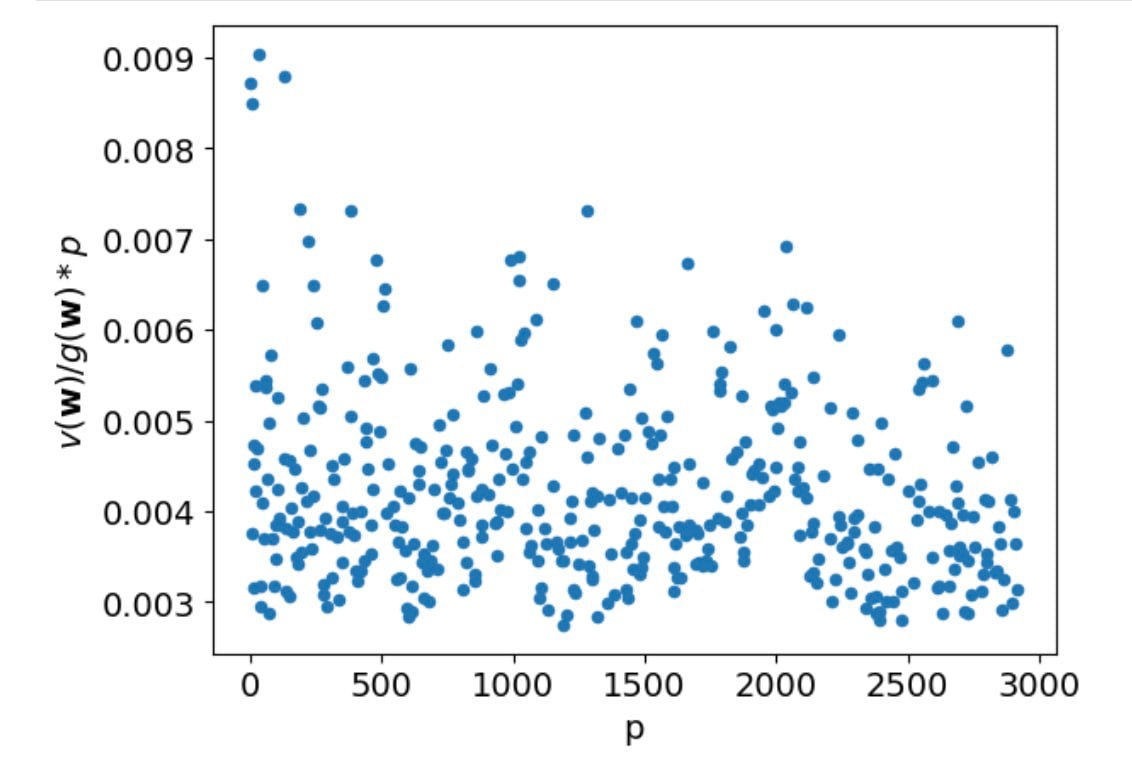
Figure 4: $\operatorname*{\mathbb{E}}_{i\sim\{1,\ldots,20\}}\left[\frac{v(\mathbf{w}_{i})}{g(\mathbf{w}_{i})}\cdot p\right]$ against $p$ for modular multiplication.

Failure to learn modular multiplication.

According to Remark 3, any gradient-based method most likely will fail to learn the parity bit of modular multiplication. To test this claim, we generated a labeled sample

$$(x_{1},(-1)^{a\cdot x_{1}}),\ldots,(x_{m},(-1)^{a\cdot x_{m}})$$

where $x_{1},\ldots,x_{m}$, and $a$ are taken randomly from $\mathbb{Z}_{p}^{\ast}$. Using this sample, we trained a dense 3-layer neural network with 1000 neurons in each hidden layer. We used Adam with a learning rate of 0.001 (default), $m=5000$, a 70/30 split between training and test sets, batch size 100, and we trained for 2000 epochs. The results for different bitlengths $n$ are shown in Figure 3. The prime base $p$ for each bitlength $n$ was taken randomly from the prime numbers in the interval $[2^{n-1},2^{n}-1]$. We can see that as the bit length increases, the chances of successful learning decrease, as predicted by our theory.

3.1 Additional Experiments

Here we present the results of experiments on the learnability of modular multiplication itself and of all its bits.

Low correlation of multiplication by different numbers.

We computed the mean squared covariance

$$\operatorname*{\mathbb{E}}_{A,B\sim\mathbb{Z}_{p}^{\ast}}\left(\operatorname*{\mathrm{Cov}}_{X\sim\mathbb{Z}_{p}^{\ast}}[A\cdot X,B\cdot X]\right)^{2}$$ (10)

for prime numbers in the interval $[3,500]$. The results are shown in Figure 5.

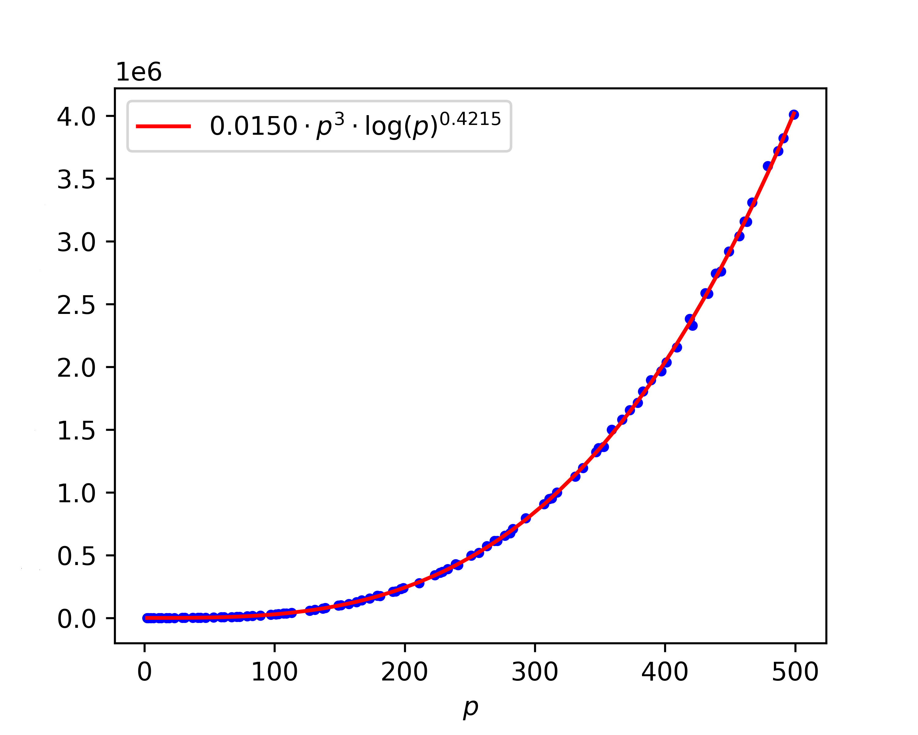
Figure 5: Mean squared covariance between two multiplications, $a\cdot X$ and $b\cdot X$, when $X$ is a random variable uniformly distributed on $\mathbb{Z}_{p}^{\ast}$.

As we can see, the expression (10) fits the curve $p\mapsto 0.015\cdot p^{3}\cdot(\log p)^{0.42}$ well. In Corollary 14 of subsection 6.1 we prove a slightly weaker bound $\operatorname*{\mathbb{E}}_{A,B\sim\mathbb{Z}_{p}^{\ast}}\left(\operatorname*{\mathrm{Cov}}_{X\sim\mathbb{Z}_{p}^{\ast}}[A\cdot X,B\cdot X]\right)^{2}\ll p^{3}\log^{2}p$. This suggests that $\operatorname*{\mathrm{Cov}}_{X\sim\mathbb{Z}_{p}^{\ast}}[a\cdot X,b\cdot X]=\tilde{\mathcal{O}}(p^{3/2})$ on average over $a,b\in\mathbb{Z}_{p}^{\ast}$. Since the variance of the multiplication by $a$ modulo $p$ is

$$\operatorname*{\mathrm{Var}}_{X\sim\mathbb{Z}_{p}^{\ast}}[a\cdot X]=\frac{1}{p-1}\sum_{k=1}^{p-1}k^{2}-\left(\frac{1}{p-1}\sum_{k=1}^{p-1}k\right)^{2}=\frac{p^{2}}{12}-\frac{p}{6}=\mathcal{O}(p^{2})$$

we have that the average correlation is

$$\operatorname*{\mathrm{Corr}}_{X\sim\mathbb{Z}_{p}^{\ast}}[a\cdot X,b\cdot X]=\tilde{\mathcal{O}}\left(\frac{1}{\sqrt{p}}\right).$$ (11)

Thus, using this estimate in the Boas-Bellman inequality for the class of “standardized” modular multiplication functions $\{f_{a}(x)\mid a\in\mathbb{Z}_{p}^{\ast}\}$, where

$$f_{a}(x)=\frac{a\cdot x-\frac{p}{2}}{\sqrt{\frac{p^{2}}{12}-\frac{p}{6}}},\qquad x\in\mathbb{Z}_{p}^{\ast},$$

one can show that this class is also hard to learn by gradient-based methods. A rigorous proof of the bound (11), together with the concentration of the gradient (Theorem 15), can be found in subsection 6.1.

Failure to learn all bits of modular multiplication.

Here we follow the experimental setup for the target $x\to[a\cdot x]_{1}$ with the difference that the output of the neural network is not only the parity bit, but all the bits of modular multiplication. As a loss function, we use the sum of the cross-entropies for each bit. The results for two different bit lengths are shown in Figure 6.

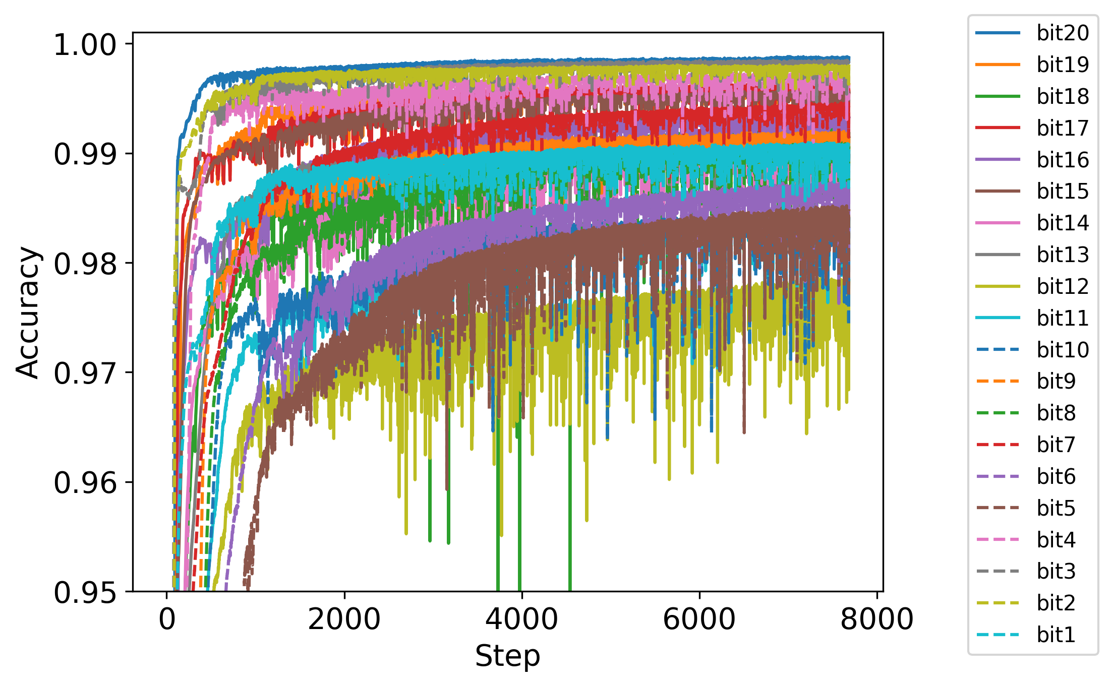
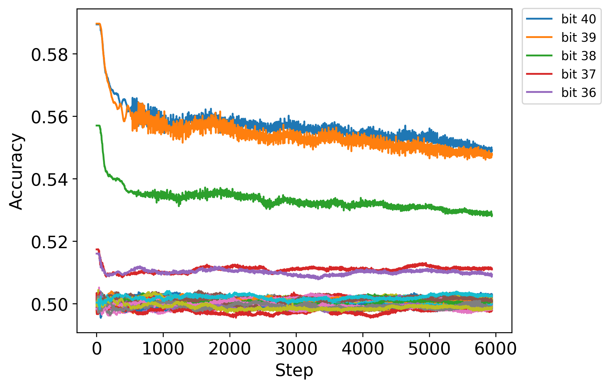
Figure 6: Test Accuracies when learning all bits of multiplication modulo $p$ with a single neural network. Bitlengths of $p$: 20 (left) and 40 (right). Accuracies are higher for larger $r$ because the classes are unbalanced.

As in the case of one bit, we see that for a longer bit length, the gradient method is not able to learn all the bits of modular multiplication.

4 High-frequency waves on the real line

Let $L_{2}([0,1])$ be a space square-integrable functions on $[0,1]$ with the inner product $\langle f,g\rangle=\int_{0}^{1}f(x)g(x)dx$. For a function with a bounded variation $f:{\mathbb{R}}\to{\mathbb{R}}$, we denote

$$\|f\|_{BV}=\sup_{0=x_{0}\leq...\leq x_{N}=1}\sum_{i=1}^{N}|f(x_{i})-f(x_{i-1})|.$$

Let $\psi:{\mathbb{R}}\to{\mathbb{R}}$ be a periodic function with period 1, i.e. $\psi(x+1)=\psi(x)$, and mean 0, i.e. $\int_{0}^{1}\psi(x)dx=0$. Also, we assume that $\psi$ has a bounded variation, i.e. $\|\psi\|_{BV}<+\infty$.

For $A\in{\mathbb{N}}$, let us introduce the hypothesis space

$$\begin{split}\mathcal{H}_{A}=\{h_{a}:{\mathbb{R}}\to{\mathbb{R}}\mid h_{a}(x)=\psi(ax),a\in{\mathbb{Z}}_{A}\}.\end{split}$$

Let $p:\mathcal{O}\times{\mathbb{R}}\to{\mathbb{R}}$ be a smooth function, where $\mathcal{O}$ is an open set in ${\mathbb{R}}^{s}$. The variance of the gradient w.r.t. $\mathcal{H}_{A}$ is defined as

$$\begin{split}{\rm Var}(\mathcal{H}_{A},{\mathbf{w}})={\rm Var}_{a\sim{\mathbb{Z}}_{A}}\big{[}\nabla_{\mathbf{w}}\|p({\mathbf{w}},x)-h_{a}(x)\|^{2}_{L_{2}([0,1])}\big{]},{\mathbf{w}}\in\mathcal{O}.\end{split}$$

We assume that the variance of a random vector is a sum of the variances of components. Let us denote $\frac{\partial p({\mathbf{w}},x)}{\partial w_{i}}\in L_{2}([0,1])$ by $g_{i}({\mathbf{w}})$ and set $g({\mathbf{w}})=[g_{1}({\mathbf{w}}),\cdots,g_{s}({\mathbf{w}})]^{\top}$. Note that $g({\mathbf{w}})\in L^{s}_{2}([0,1])$ and we assume $\|g({\mathbf{w}})\|^{2}_{L^{s}_{2}([0,1])}=\sum_{i=1}^{s}\|g_{i}({\mathbf{w}})\|^{2}_{L_{2}([0,1])}$. The following theorem shows that for a large $A$, the variance of the gradient w.r.t. $\mathcal{H}_{A}$ is very small.

Theorem 1.

There exists a universal constant $C>0$ such that

$$\begin{split}{\rm Var}(\mathcal{H}_{A},{\mathbf{w}})\leq C\|g({\mathbf{w}})\|^{2}_{L^{s}_{2}([0,1])}\|\psi\|^{2}_{BV}A^{-1/2}(\log A+1)^{5/2}.\end{split}$$

In the proof of the latter theorem we will need the following classical fact, which is a generalization of Bessel’s inequality.

Lemma 2 (Boas-Bellman inequality).

Let $h_{1},\ldots,h_{m},g$ be elements of a some Hilbert space $\mathcal{H}$ equipped with the inner product $\langle\cdot,\cdot\rangle_{\mathcal{H}}$. Then

$$\sum_{i=1}^{m}\langle h_{i},g\rangle^{2}_{\mathcal{H}}\leq\|g\|^{2}_{\mathcal{H}}\left(\max_{i}\|h_{i}\|^{2}_{\mathcal{H}}+\sqrt{\sum_{i\neq j}\langle h_{i},h_{j}\rangle^{2}_{\mathcal{H}}}\right).$$

Proof of Theorem 1.

The variance of the gradient w.r.t. $\mathcal{H}_{A}$ can be bounded in the following way:

$$\begin{split}{\rm Var}_{a\sim{\mathbb{Z}}_{A}}\big{[}\partial_{w_{i}}{\mathbb{E}}_{x\sim[0,1]}[(p({\mathbf{w}},x)-h_{a}(x))^{2}]\big{]}={\rm Var}_{a\sim{\mathbb{Z}}_{A}}\big{[}{\mathbb{E}}_{x\sim[0,1]}[2(p({\mathbf{w}},x)-h_{a}(x))\partial_{w_{i}}p({\mathbf{w}},x)]\big{]}=\\ 4{\rm Var}_{a\sim{\mathbb{Z}}_{A}}\big{[}{\mathbb{E}}_{x\sim[0,1]}[h_{a}(x)\partial_{w_{i}}p({\mathbf{w}},x)]\big{]}\leq\frac{4}{A}\sum_{a\in{\mathbb{Z}}_{A}}\langle h_{a},g_{i}({\mathbf{w}})\rangle^{2}.\end{split}$$

The Boas-Bellmann inequality gives us

$$\begin{split}\sum_{a=0}^{A-1}\langle h_{a},g_{i}({\mathbf{w}})\rangle^{2}\leq\|g_{i}({\mathbf{w}})\|^{2}_{L_{2}([0,1])}\big{(}\max_{a\in{\mathbb{Z}}_{A}}\|h_{a}\|^{2}+\sqrt{\sum_{a\neq b\in{\mathbb{Z}}_{A}}\langle h_{a},h_{b}\rangle^{2}}\big{)}.\end{split}$$ (12)

Recall that $\langle h_{a},h_{b}\rangle=\int_{0}^{1}\psi(ax)\psi(bx)dx$. Therefore,

$$\begin{split}\sum_{a,b\in{\mathbb{Z}}_{A}}\langle h_{a},h_{b}\rangle^{2}=\sum_{a,b\in{\mathbb{Z}}_{A}}\int_{[0,1]^{2}}\psi(ax)\psi(bx)\psi(ay)\psi(by)dxdy=\int_{[0,1]^{2}}Q(x,y)^{2}dxdy=\|Q\|^{2}_{L_{2}([0,1]^{2})}.\end{split}$$ (13)

where $Q(x,y)=\sum_{a\in{\mathbb{Z}}_{A}}\psi(ax)\psi(ay)$. This function can be represented as

$$Q(x,y)=\sum_{a=0}^{A-1}\psi^{2}(T^{a}_{(x,y)}(0,0)),$$

where $C={\mathbb{R}}/{\mathbb{Z}}$ is a factor-group (topologically isomorphic to a circle), $\psi^{2}:C\times C\to{\mathbb{R}}$, $\psi^{2}(x^{\prime},y^{\prime})=\psi(x^{\prime})\psi(y^{\prime})$ and $T_{(x,y)}:C\times C\to C\times C$, $T_{(x,y)}(x^{\prime},y^{\prime})=(x^{\prime}+x\bmod 1,y^{\prime}+y\bmod 1)$, $T^{a}_{(x,y)}=T_{(x,y)}\circ\cdots\circ T_{(x,y)}$ ($a$ times). The Weyl-von Neumann theorem guarantees that the mapping $T_{(x,y)}$ is ergodic on the 2-dimensional torus $C\times C$ if $ax+by=c,a,b,c\in{\mathbb{Z}}$ implies $a=b=c=0$. Thus, almost surely the following is satisfied:

$$\begin{split}\lim_{A\to+\infty}\frac{1}{A}\sum_{a=0}^{A-1}\psi^{2}(T^{a}_{(x,y)}(0,0))=\int_{[0,1]^{2}}\psi(x^{\prime})\psi(y^{\prime})dx^{\prime}dy^{\prime}=0.\end{split}$$

The Erdős-Turán-Koksma inequality (see pages 116 and 151 of [20]) helps us to bound the speed of convergence, i.e.

$$\begin{split}|\frac{1}{A}\sum_{a=0}^{A-1}\psi^{2}(T^{a}_{(x,y)}(0,0))|\ll\|\psi\|^{2}_{BV}\big{(}\frac{2}{H+1}+\sum_{a,b\in[-H,H]\cap{\mathbb{Z}},(a,b)\neq(0,0)}\frac{\frac{1}{A}|\sum_{n=0}^{A-1}e^{2\pi{\rm i}(anx+bny)}|}{\max(1,|a|)\max(1,|b|)}\big{)},\end{split}$$

for any $H\in{\mathbb{N}}$. Since $\sum_{n=0}^{A-1}e^{2\pi{\rm i}(anx+bny)}=\frac{e^{2\pi{\rm i}A(ax+by)}-1}{e^{2\pi{\rm i}(ax+by)}-1}$, we conclude

$$\begin{split}\|Q\|^{2}_{L_{2}([0,1]^{2})}\ll\\ A^{2}\|\psi\|^{4}_{BV}{\mathbb{E}}_{(x,y)\sim[0,1]^{2}}\big{(}\frac{2}{H+1}+\sum_{a,b\in[-H,H]\cap{\mathbb{Z}},(a,b)\neq(0,0)}\frac{|\sin(\pi A(ax+by))|}{A|\sin(\pi(ax+by))|\max(1,|a|)\max(1,|b|)}\big{)}^{2}.\end{split}$$ (14)

Now our plan will be to estimate the latter expression and obtain an upper bound on $\|Q\|^{2}_{L_{2}([0,1]^{2})}$. Further, we will combine it with the equality (13) and bound the expression $\sum_{a,b\in{\mathbb{Z}}_{A}}\langle h_{a},h_{b}\rangle^{2}$. The last expression bounds the needed variance according to Boas-Bellman inequality (12).

The following lemma is a key fact behind our bound of the RHS of (14).

Lemma 3.

For $\omega\geq 1,r\in{\mathbb{N}}$, we have $\int_{-1}^{1}\frac{|\sin(r\omega x)|}{|\sin(\omega x)|}dx\ll 1+\log r$.

Proof.

First note that if $\omega x\notin\Omega$ where $\Omega=\bigcup_{k\in{\mathbb{Z}}}(\pi k\pm\frac{\pi}{4})$, then $\frac{|\sin(r\omega x)|}{|\sin(\omega x)|}\leq\sqrt{2}$ and $\int_{[-1,1]\setminus\Omega}\frac{|\sin(r\omega x)|}{|\sin(\omega x)|}dx\leq 2\sqrt{2}$.

Let us now estimate $\int_{[-1,1]\cap\Omega}\frac{|\sin(r\omega x)|}{|\sin(\omega x)|}dx$. If $\omega x\in\pi k\pm\frac{\pi}{4}$, then $2|\sin(\omega x)|\geq|\omega x-\pi k|$. We have

$$\begin{split}\int_{(\pi k\pm\frac{\pi}{4})/\omega}\frac{|\sin(r\omega x)|}{|\sin(\omega x)|}dx\leq 2\int_{(\pi k\pm\frac{\pi}{4})/\omega}\frac{|\sin(r(\omega x-\pi k))|}{|\omega x-\pi k|}dx=\\ \frac{2}{\omega}\int_{-\pi/4}^{\pi/4}\frac{|\sin(rx)|}{|x|}dx=\frac{2}{\omega}\int_{-r\pi/4}^{r\pi/4}\frac{|\sin(x)|}{|x|}dx\ll\frac{\log r+1}{\omega}.\end{split}$$

Since the number $|k|$ can be at most $\lfloor\frac{\omega+\frac{\pi}{4}}{\pi}\rfloor$, the total integral is asymptotically bounded by $1+\frac{\log r+1}{\omega}\frac{\omega+\frac{\pi}{4}}{\pi}\ll 1+\log r$. ∎

Lemma 4.

For $(a,b)\in{\mathbb{Z}}^{2}\setminus\{(0,0)\}$, we have ${\mathbb{E}}_{(x,y)\sim[0,1]^{2}}[\frac{|\sin(\pi A(ax+by))|}{|\sin(\pi(ax+by))|}]\ll 1+\log A$.

Proof.

The following chain of inequalities can be checked:

$$\begin{split}{\mathbb{E}}_{(x,y)\sim[0,1]^{2}}\big{[}\frac{|\sin(\pi A(ax+by))|}{|\sin(\pi(ax+by))|}\big{]}\leq\int_{x^{2}+y^{2}\leq 2}\frac{|\sin(\pi A(ax+by))|}{|\sin(\pi(ax+by))|}dxdy=\\ \frac{1}{a^{2}+b^{2}}\int_{x^{2}+y^{2}\leq 2(a^{2}+b^{2})}\frac{|\sin(\pi Ax)|}{|\sin(\pi x)|}dxdy=\frac{1}{a^{2}+b^{2}}\int_{-\sqrt{2(a^{2}+b^{2})}}^{\sqrt{2(a^{2}+b^{2})}}\frac{|\sin(\pi Ax)|\sqrt{2(a^{2}+b^{2})-x^{2}}}{|\sin(\pi x)|}dx\leq\\ \frac{\sqrt{2}}{\sqrt{a^{2}+b^{2}}}\int_{-\sqrt{2(a^{2}+b^{2})}}^{\sqrt{2(a^{2}+b^{2})}}\frac{|\sin(\pi Ax)|}{|\sin(\pi x)|}dx=2\int_{-1}^{1}\frac{|\sin(\pi A\sqrt{2a^{2}+2b^{2}}x)|}{|\sin(\pi\sqrt{2a^{2}+2b^{2}}x)|}dx.\end{split}$$

Using Lemma 3 we conclude that the latter expression is asymptotically bounded by $1+\log A$. ∎

Lemma 5.

For $(a,b),(c,d)\in{\mathbb{Z}}^{2}\setminus\{(0,0)\}$, we have ${\mathbb{E}}_{(x,y)\sim[0,1]^{2}}[\frac{|\sin(\pi A(ax+by))\sin(\pi A(cx+dy))|}{|\sin(\pi(ax+by))\sin(\pi(cx+dy))|}]\ll A(1+\log A)$.

Proof.

Using $\frac{|\sin(\pi A(cx+dy))|}{|\sin(\pi(cx+dy))|}\leq A$ and the previous lemma, we obtain

$$\begin{split}{\mathbb{E}}_{(x,y)\sim[0,1]^{2}}[\frac{|\sin(\pi A(ax+by))\sin(\pi A(cx+dy))|}{|\sin(\pi(ax+by))\sin(\pi(cx+dy))|}]\leq A{\mathbb{E}}_{(x,y)\sim[0,1]^{2}}\big{[}\frac{|\sin(\pi A(ax+by))|}{|\sin(\pi(ax+by))|}\big{]}\ll A(1+\log A).\end{split}$$

∎

Now we are ready to bound $\|Q\|^{2}_{L_{2}([0,1]^{2})}$ using (14) and Lemmas 4 and 5 by:

$$\begin{split}{\mathbb{E}}_{(x,y)\sim[0,1]^{2}}\big{(}\frac{2}{H+1}+\sum_{\scriptscriptstyle a,b\in[-H,H]\cap{\mathbb{Z}},(a,b)\neq(0,0)}\frac{|\sin(\pi A(ax+by))|}{A|\sin(\pi(ax+by))|\max(1,|a|)\max(1,|b|)}\big{)}^{2}=\end{split}$$

$$\begin{split}\frac{4}{(H+1)^{2}}+\frac{4}{H+1}\sum_{\scriptscriptstyle a,b\in[-H,H]\cap{\mathbb{Z}},(a,b)\neq(0,0)}{\mathbb{E}}_{(x,y)\sim[0,1]^{2}}\frac{|\sin(\pi A(ax+by))|}{A|\sin(\pi(ax+by))|\max(1,|a|)\max(1,|b|)}\\ +A^{-2}\sum_{\begin{subarray}{c}\scriptscriptstyle a,b\in[-H,H]\cap{\mathbb{Z}},(a,b)\neq(0,0)\\ \scriptscriptstyle c,d\in[-H,H]\cap{\mathbb{Z}},(c,d)\neq(0,0)\end{subarray}}\frac{1}{\max(1,|a|)\max(1,|b|)\max(1,|c|)\max(1,|d|)}\\ \times{\mathbb{E}}_{(x,y)\sim[0,1]^{2}}[\frac{|\sin(\pi A(ax+by))\sin(\pi A(cx+dy))|}{|\sin(\pi(ax+by))\sin(\pi(cx+dy))|}]\ll\end{split}$$

$$\begin{split}H^{-2}+H^{-1}A^{-1}(\log A+1)(\sum_{a=-H}^{H}\frac{1}{\max(1,|a|)})^{2}+A^{-1}(\log A+1)(\sum_{a=-H}^{H}\frac{1}{\max(1,|a|)})^{4}\ll\\ H^{-2}+H^{-1}A^{-1}(\log A+1)(\log H+1)^{2}+A^{-1}(\log A+1)(\log H+1)^{4}.\end{split}$$

After we set $H\asymp A^{1/2}(\log A+1)^{-5/2}$ we obtain

$$\|Q\|^{2}_{L_{2}([0,1]^{2})}\ll A^{2}\|\psi\|^{4}_{BV}A^{-1}(\log A+1)^{5}.$$ (15)

Finally, using (12), we obtain

$$\begin{split}\sum_{a=0}^{A-1}\langle h_{a},g_{i}({\mathbf{w}})\rangle^{2}\leq\|g_{i}({\mathbf{w}})\|^{2}_{L_{2}([0,1])}\big{(}\max_{a\in{\mathbb{Z}}_{A}}\|h_{a}\|^{2}+\sqrt{\|Q\|^{2}_{L_{2}([0,1]^{2})}}\big{)}\ll\\ \|g_{i}({\mathbf{w}})\|^{2}_{L_{2}([0,1])}\big{(}\|\psi\|^{2}_{BV}+\|\psi\|^{2}_{BV}A^{1/2}(\log A+1)^{5/2}\big{)}.\end{split}$$

The latter directly implies

$$\begin{split}{\rm Var}_{a\sim{\mathbb{Z}}_{A}}\big{[}\nabla_{\mathbf{w}}{\mathbb{E}}_{x}(p_{w}(x)-h_{a}(x))^{2}\big{]}\ll\|g({\mathbf{w}})\|^{2}_{L^{s}_{2}([0,1])}A^{-1}\big{(}\|\psi\|^{2}_{BV}+\|\psi\|^{2}_{BV}A^{1/2}(\log A+1)^{5/2}\big{)}\\ \ll\|g({\mathbf{w}})\|^{2}_{L^{s}_{2}([0,1])}\|\psi\|^{2}_{BV}A^{-1/2}(\log A+1)^{5/2}.\end{split}$$

∎

5 The case of $p$-periodic function on ${\mathbb{Z}}$

Let $t:{\mathbb{Z}}^{\ast}_{p}\to{\mathbb{R}}$ be some function. Let us extend this function to ${\mathbb{Z}}_{p}$ by defining $t(0)$ arbitrarily. Let $a\in{\mathbb{Z}}_{p}^{\ast}$. Let us define a function $\mathring{h}_{a}:{\mathbb{Z}}_{p}\to{\mathbb{R}}$ by

$$\mathring{h}_{a}(x)=t(a\cdot x),$$ (16)

and define a hypothesis set

$$\mathring{\mathcal{H}}_{p}=\{\mathring{h}_{a}(x)\mid a\in{\mathbb{Z}}_{p}^{\ast}\}.$$ (17)

Throughout the section we assume that elements of ${\mathbb{R}}^{p}$ (or, ${\mathbb{C}}^{p}$) are functions from ${\mathbb{Z}}_{p}$ to ${\mathbb{R}}$ (or, ${\mathbb{C}}$) and introduce an inner product in ${\mathbb{R}}^{p}$ (or, ${\mathbb{C}}^{p}$) by

$$\langle f,g\rangle=\sum_{x\in{\mathbb{Z}}_{p}}f(x)^{\dagger}g(x).$$

We will be interested in the variance of the gradient w.r.t. $\mathring{\mathcal{H}}_{p}$ defined by

$${\rm Var}(\mathring{\mathcal{H}}_{p},{\mathbf{w}})={\rm Var}_{A\sim{\mathbb{Z}}^{\ast}_{p}}\big{[}\nabla_{\mathbf{w}}{\mathbb{E}}_{x\sim{\mathbb{Z}}^{\ast}_{p}}[L(\mathring{h}_{A}(x),p({\mathbf{w}},x))]\big{]},$$ (18)

where $L$ is either a square loss function (for regression tasks) or $L(y,y^{\prime})=l(yy^{\prime})$, where $l$ is some 1-Lipschitz function (for binary classification tasks).

Again, let $p({\mathbf{w}},x)$ depend smoothly on $w$ and let us denote $\partial_{w_{i}}p({\mathbf{w}},x)\in{\mathbb{R}}^{p}$ by $g_{i}({\mathbf{w}})$. A natural norm of the gradient is given by $\|g_{i}\|^{2}_{\ast}={\mathbb{E}}_{X\sim{\mathbb{Z}}_{p}}\big{[}(\partial_{w_{i}}p({\mathbf{w}},X))^{2}\big{]}$. Also, let $g({\mathbf{w}})=[g_{1}({\mathbf{w}}),\cdots,g_{s}({\mathbf{w}})]^{\top}$ and $\|g\|^{2}_{\ast s}=\sum_{i=1}^{s}\|g_{i}\|_{\ast}^{2}$.

Theorem 6.

For the square loss function, we have

$$\begin{split}{\rm Var}_{a\sim{\mathbb{Z}}^{\ast}_{p}}\big{[}\nabla_{\mathbf{w}}{\mathbb{E}}_{x\sim{\mathbb{Z}}^{\ast}_{p}}[L(\mathring{h}_{a}(x),p({\mathbf{w}},x))]\big{]}\ll\|g({\mathbf{w}})\|^{2}_{\ast s}\sqrt{{\mathbb{E}}_{Y\sim\mathbb{Z}_{p}^{\ast}}[f(Y)^{2}]},\end{split}$$ (19)

where

$$f(Y)=\frac{1}{p-1}\sum_{x\in{\mathbb{Z}}_{p}^{\ast}}t(x)t(Y\cdot x).$$ (20)

Proof.

Since the l.h.s. does not depend on the value of $t$ at 0, we can set $t(0)=0$. In the case of the square loss, an application of the Boas-Bellman inequality to the family $\{\mathring{h}_{a}(x)\}_{a\in{\mathbb{Z}}_{p}^{\ast}}$ gives us

$$\begin{split}{\rm Var}_{A\sim{\mathbb{Z}}^{\ast}_{p}}\big{[}\partial_{w_{i}}{\mathbb{E}}_{x\sim{\mathbb{Z}}^{\ast}_{p}}[(\mathring{h}_{A}(x)-p({\mathbf{w}},x))^{2}]\big{]}\leq\frac{4}{(p-1)^{2}}{\mathbb{E}}_{A\sim{\mathbb{Z}}_{p}^{\ast}}\big{[}\langle t(A\cdot x),g_{i}(w,x)\rangle^{2}\big{]}=\\ \frac{4}{(p-1)^{3}}\sum_{a\in{\mathbb{Z}}_{p}^{\ast}}\langle t(a\cdot x),g_{i}(w,x)\rangle^{2}\leq\frac{4\|g_{i}({\mathbf{w}})\|^{2}}{(p-1)^{3}}\big{(}\max_{a\in{\mathbb{Z}}_{p}^{\ast}}\|\mathring{h}_{a}\|^{2}+\sqrt{\sum_{a\neq b}\langle\mathring{h}_{a},\mathring{h}_{b}\rangle^{2}}\big{)}.\end{split}$$ (21)

Note that the r.h.s. is bounded by a factor of $\sqrt{\sum_{a,b\in{\mathbb{Z}}_{p}^{\ast}}\langle\mathring{h}_{a},\mathring{h}_{b}\rangle^{2}}$. As the following lemma shows, it is itself can be bounded by a factor of $\sqrt{{\mathbb{E}}_{Y\sim\mathbb{Z}_{p}^{\ast}}[f(Y)^{2}]}$.

Lemma 7.

We have,

$$\begin{split}\sum_{a\in{\mathbb{Z}}_{p}^{\ast}}\sum_{b\in{\mathbb{Z}}_{p}^{\ast}}\langle\mathring{h}_{a},\mathring{h}_{b}\rangle^{2}=(p-1)^{4}{\mathbb{E}}_{Y\sim\mathbb{Z}_{p}^{\ast}}[f(Y)^{2}].\end{split}$$

Proof of Lemma.

The following sequence of identities can be directly checked:

$$\begin{split}\frac{1}{(p-1)^{2}}\sum_{a\in{\mathbb{Z}}_{p}^{\ast}}\sum_{b\in{\mathbb{Z}}_{p}^{\ast}}{\mathbb{E}}_{X\sim{\mathbb{Z}}_{p}^{\ast}}[\mathring{h}_{a}(X)\mathring{h}_{b}(X)]^{2}=\operatorname*{\mathbb{E}}_{A,B\sim{\mathbb{Z}}_{p}^{\ast}}\left[\operatorname*{\mathbb{E}}_{X\sim{\mathbb{Z}}_{p}^{\ast}}[\mathring{h}_{A}(X)\mathring{h}_{B}(X)]^{2}\right]\\ =\operatorname*{\mathbb{E}}_{A,B\sim{\mathbb{Z}}_{p}^{\ast}}\left[\operatorname*{\mathbb{E}}_{X\sim{\mathbb{Z}}_{p}^{\ast}}\left[t(AX)t(BX)\right]^{2}\right]=\operatorname*{\mathbb{E}}_{A,B\sim{\mathbb{Z}}_{p}^{\ast}}\left[\operatorname*{\mathbb{E}}_{X\sim{\mathbb{Z}}_{p}^{\ast}}\left[t(AX)t((B\cdot A^{-1})\cdot AX)\right]^{2}\right]\\ \end{split}$$

$$\begin{split}=\operatorname*{\mathbb{E}}_{A,B\sim{\mathbb{Z}}_{p}^{\ast}}\left[\operatorname*{\mathbb{E}}_{X\sim{\mathbb{Z}}_{p}^{\ast}}\left[t(X)t((B\cdot A^{-1})\cdot X)\right]^{2}\right]=\operatorname*{\mathbb{E}}_{Y\sim{\mathbb{Z}}_{p}^{\ast}}\left[\operatorname*{\mathbb{E}}_{X\sim\mathbb{Z}_{p}^{\ast}}\left[t(X)t(Y\cdot X)\right]^{2}\right]=\\ {\mathbb{E}}_{Y\sim\mathbb{Z}_{p}^{\ast}}[f(Y)^{2}].\end{split}$$

Since ${\mathbb{E}}_{X\sim{\mathbb{Z}}_{p}^{\ast}}[\mathring{h}_{a}(X)\mathring{h}_{b}(X)]=\frac{\langle\mathring{h}_{a},\mathring{h}_{b}\rangle}{p-1}$, we conclude $\sum_{a,b\in{\mathbb{Z}}_{p}^{\ast}}\langle\mathring{h}_{a},\mathring{h}_{b}\rangle^{2}=(p-1)^{4}{\mathbb{E}}_{Y\sim\mathbb{Z}_{p}^{\ast}}[f(Y)^{2}]$. Lemma proved. ∎

Thus, we have

$$\begin{split}{\rm Var}_{a\sim{\mathbb{Z}}^{\ast}_{p}}\big{[}\partial_{w_{i}}{\mathbb{E}}_{x\sim{\mathbb{Z}}^{\ast}_{p}}[(\mathring{h}_{a}(x)-p({\mathbf{w}},x))^{2}]\big{]}\ll\|g_{i}({\mathbf{w}})\|^{2}_{\ast}\sqrt{{\mathbb{E}}_{Y\sim\mathbb{Z}_{p}^{\ast}}[f(Y)^{2}]},\end{split}$$

from which the statement of the theorem for a square loss function directly follows. ∎

Using ideas from Appendix B.1 of [10], the case of a binary classification task and a 1-Lipschitz loss can be treated analogously. Let us give a proof of the following theorem for completeness.

Theorem 8.

Suppose that $t(x)=t_{1}(x)+c,x\in{\mathbb{Z}}^{\ast}_{p}$ and a restriction of $t$ to ${\mathbb{Z}}^{\ast}_{p}$ is $\{-1,1\}$-valued. For $L(y,y^{\prime})=l(yy^{\prime})$, where $l$ is some 1-Lipschitz function, we have

$$\begin{split}{\rm Var}_{a\sim{\mathbb{Z}}^{\ast}_{p}}\big{[}\nabla_{\mathbf{w}}{\mathbb{E}}_{x\sim{\mathbb{Z}}^{\ast}_{p}}[L(\mathring{h}_{a}(x),p({\mathbf{w}},x))]\big{]}\ll\|g({\mathbf{w}})\|^{2}_{\ast s}\sqrt{{\mathbb{E}}_{Y\sim\mathbb{Z}_{p}^{\ast}}[f_{1}(Y)^{2}]},\end{split}$$ (22)

where $f_{1}(y)={\mathbb{E}}_{X\sim{\mathbb{Z}}_{p}^{\ast}}t_{1}(X)t_{1}(y\cdot X)$.

Proof.

W.l.o.g. $t(0)=t_{1}(0)=0$. We have

$$\begin{split}{\rm Var}_{a\sim{\mathbb{Z}}^{\ast}_{p}}\big{[}\partial_{w_{i}}{\mathbb{E}}_{x\sim{\mathbb{Z}}^{\ast}_{p}}[l(t(a\cdot x)p({\mathbf{w}},x))]\big{]}={\rm Var}_{a\sim{\mathbb{Z}}^{\ast}_{p}}\big{[}{\mathbb{E}}_{x\sim{\mathbb{Z}}^{\ast}_{p}}[\partial_{w_{i}}p({\mathbf{w}},x)l^{\prime}(t(a\cdot x)p({\mathbf{w}},x))]\big{]}=\\ {\rm Var}_{a\sim{\mathbb{Z}}^{\ast}_{p}}\big{[}{\mathbb{E}}_{x\sim{\mathbb{Z}}^{\ast}_{p}}[\partial_{w_{i}}p({\mathbf{w}},x)(\frac{l^{\prime}(p({\mathbf{w}},x))+l^{\prime}(-p({\mathbf{w}},x))}{2}+\frac{l^{\prime}(p({\mathbf{w}},x))-l^{\prime}(-p({\mathbf{w}},x))}{2}t(a\cdot x))]\big{]}=\\ {\rm Var}_{a\sim{\mathbb{Z}}^{\ast}_{p}}\big{[}{\mathbb{E}}_{x\sim{\mathbb{Z}}^{\ast}_{p}}[\partial_{w_{i}}p({\mathbf{w}},x)\frac{l^{\prime}(p({\mathbf{w}},x))-l^{\prime}(-p({\mathbf{w}},x))}{2}t_{1}(a\cdot x)]\big{]}\leq{\mathbb{E}}_{a\sim{\mathbb{Z}}^{\ast}_{p}}\big{[}{\mathbb{E}}_{x\sim{\mathbb{Z}}^{\ast}_{p}}[H({\mathbf{w}},x)t_{1}(a\cdot x)]^{2}\big{]}.\end{split}$$ (23)

where $H({\mathbf{w}},x)=\partial_{w_{i}}p({\mathbf{w}},x)\frac{l^{\prime}(p({\mathbf{w}},x))-l^{\prime}(-p({\mathbf{w}},x))}{2}$. Let us fix ${\mathbf{w}}$ and treat $H({\mathbf{w}},x)$ as a vector from ${\mathbb{R}}^{p}$. Using the Boas-Bellman inequality we bound the latter expression by $\frac{4\|H({\mathbf{w}},x)\|^{2}}{(p-1)^{3}}\big{(}\max_{a\in{\mathbb{Z}}_{p}^{\ast}}\|t_{1}(a\cdot x)\|^{2}+\sqrt{\sum_{a\neq b}\langle t_{1}(a\cdot x),t_{1}(b\cdot x)\rangle^{2}}\big{)}$. Using 1-Lipschitzness of $l$, we have $\|H({\mathbf{w}},x)\|^{2}\leq\|g_{i}({\mathbf{w}})\|^{2}$. Further, we proceed identically to the proof of the squared loss case. ∎

Next, our goal will be to find conditions under which $f(Y)$ is concentrated around its mean, whose value is established by the following theorem.

Theorem 9.

${\mathbb{E}}_{Y\sim{\mathbb{Z}}^{\ast}_{p}}[f(Y)]={\mathbb{E}}_{X\sim{\mathbb{Z}}^{\ast}_{p}}[t(X)]^{2}$.

Proof.

The following chain of identities can be easily verified.

$$\begin{split}{\mathbb{E}}_{Y\sim{\mathbb{Z}}^{\ast}_{p}}[f(Y)]={\mathbb{E}}_{Y\sim{\mathbb{Z}}^{\ast}_{p}}{\mathbb{E}}_{X\sim{\mathbb{Z}}^{\ast}_{p}}[t(X)t(Y\cdot X)]=\\ {\mathbb{E}}_{X\sim{\mathbb{Z}}^{\ast}_{p}}{\mathbb{E}}_{Y\sim{\mathbb{Z}}^{\ast}_{p}}[t(X)t(Y\cdot X)]={\mathbb{E}}_{X\sim{\mathbb{Z}}^{\ast}_{p}}{\mathbb{E}}_{Y\sim{\mathbb{Z}}^{\ast}_{p}}[t(X)t(Y)]={\mathbb{E}}_{X\sim{\mathbb{Z}}^{\ast}_{p}}[t(X)]^{2}.\end{split}$$

∎

5.1 A key theorem

The goal of this subsection is to study the distribution of the random variable $f(Y)$, defined by (20), where $Y$ is sampled uniformly at random from ${\mathbb{Z}}_{p}^{\ast}$. Let us now study the second moment of $f(Y)$ (which is equal to the variance of $f(Y)$).

Lemma 10.

Let $\mathbf{\Phi}=[t(y\cdot x)]_{(x,y)\in({\mathbb{Z}}_{p}^{\ast})^{2}}$ and ${\mathbf{t}}=[t(x)]_{x\in{\mathbb{Z}}_{p}^{\ast}}$. Then, ${\mathbb{E}}[f(Y)^{2}]=\frac{1}{(p-1)^{3}}\|\mathbf{\Phi}{\mathbf{t}}\|^{2}$.

Proof.

The second moment equals

$$\begin{split}{\mathbb{E}}[f(Y)^{2}]=\frac{1}{p-1}\sum_{y\in{\mathbb{Z}}_{p}^{\ast}}\frac{1}{(p-1)^{2}}\left(\sum_{x\in{\mathbb{Z}}_{p}^{\ast}}t(x)t(x\cdot y)\right)^{2}=\\ \frac{1}{(p-1)^{3}}\sum_{(y,x,x^{\prime})\in({\mathbb{Z}}_{p}^{\ast})^{3}}t(x)t(x\cdot y)t(x^{\prime})t(x^{\prime}\cdot y)=\frac{1}{(p-1)^{3}}\|[\sum_{x\in{\mathbb{Z}}_{p}^{\ast}}t(y\cdot x)t(x)]_{y\in{\mathbb{Z}}_{p}^{\ast}}\|^{2}=\frac{1}{(p-1)^{3}}\|\mathbf{\Phi}{\mathbf{t}}\|^{2}.\end{split}$$

∎

Our next goal will be to study $\|\mathbf{\Phi}{\mathbf{t}}\|^{2}$. Let us denote the vector $[t(x)]_{x\in{\mathbb{Z}}_{p}}\in{\mathbb{R}}^{p}$ by ${\mathbf{a}}$. Let $\omega=e^{\frac{2\pi{\rm i}}{p}}$ be a primitive $p$th root of unity. Other primitive roots of unity are $\omega_{2},\cdots,\omega_{p-1}$ where $\omega_{k}=\omega^{k},k\in{\mathbb{Z}}_{p}$. The matrix $\frac{1}{\sqrt{p}}\mathbf{U}_{k}$, where $\mathbf{U}_{k}=[\omega^{ij}_{k}]_{i,j\in{\mathbb{Z}}_{p}}$, is unitary for $k\in{\mathbb{Z}}_{p}^{\ast}$. In fact, $\mathbf{U}^{\top}_{1}$ is a discrete Fourier transform (DFT) matrix. For any $h:{\mathbb{Z}}_{p}\to{\mathbb{C}}$, its DFT is defined by

$$\begin{split}\widehat{h}(y)=\sum_{x\in{\mathbb{Z}}_{p}}\omega^{-yx}h(x).\end{split}$$

Recall that $\frac{1}{\sqrt{p}}\mathbf{U}_{k}$ is a unitarity matrix. Let us denote $\mathbf{U}_{1}=\begin{bmatrix}{\mathbf{b}}_{0},\cdots,{\mathbf{b}}_{p-1}\end{bmatrix}$. Our key tool for bounding $\|\mathbf{\Phi}{\mathbf{t}}\|^{2}$ is the following theorem.

Theorem 11.

Suppose that $t(0)=\sum_{x\in{\mathbb{Z}}_{p}^{\ast}}t(x)=0$. Let $t(x)=t^{1}(x)+t^{2}(x)$ where $t_{2}(x)=c[x\neq 0]$. Then, we have

$$\begin{split}{\mathbb{E}}[f(Y)^{2}]\leq\frac{1}{p(p-1)^{3}}(\sum_{x\in{\mathbb{Z}}_{p}^{\ast}}|\widehat{t^{1}}(x)|)^{2}(\sum_{x\in{\mathbb{Z}}_{p}^{\ast}}|t(x)|^{2}).\end{split}$$

Proof.

From unitarity of ${\mathbf{U}}_{1}$, we conclude that $\left\{{\mathbf{e}}_{i}=\frac{1}{\sqrt{p}}{\mathbf{b}}_{i}\right\}_{i=0}^{p-1}$ is an orthonormal basis in ${\mathbb{C}}^{p}$. The inverse DFT can be understood as an expansion

$$\begin{split}{\mathbf{a}}=\sum_{i=0}^{p-1}({\mathbf{e}}_{i}^{\dagger}{\mathbf{a}}){\mathbf{e}}_{i}.\end{split}$$

Note that

$$\begin{split}({\mathbf{e}}_{i}^{\dagger}{\mathbf{a}})&=\frac{1}{\sqrt{p}}\sum_{x=0}^{p-1}\omega^{-xi}t(x)=\frac{1}{\sqrt{p}}\widehat{t}(i).\end{split}$$

Thus, we conclude that

$$\begin{split}{\mathbf{a}}=\sum_{i=0}^{p-1}\frac{1}{\sqrt{p}}\widehat{t}(i){\mathbf{e}}_{i}=\frac{1}{p}\sum_{i=0}^{p-1}\widehat{t}(i){\mathbf{b}}_{i}.\end{split}$$

Note that $\widehat{t}(0)=0$ due to $\sum_{x\in{\mathbb{Z}}_{p}}t(x)=0$. From the latter equation we conclude that $t(x)=\frac{1}{p}\sum_{k=1}^{p-1}\widehat{t}(k)\omega^{kx}$, and therefore $t(x\cdot y)=\frac{1}{p}\sum_{k=1}^{p-1}\widehat{t}(k)\omega^{kxy}$. Equivalently,

$$\begin{split}\mathbf{\Psi}=[t(x\cdot y)]_{(x,y)\in{\mathbb{Z}}_{p}^{2}}=\frac{1}{p}\sum_{k=1}^{p-1}\widehat{t}(k){\mathbf{U}}_{k}.\end{split}$$

Using $t(0)=0$, we have

$$\begin{split}\mathbf{\Psi}{\mathbf{a}}=t(0)^{2}\begin{bmatrix}1\\ \vdots\\ 1\end{bmatrix}+\begin{bmatrix}t(0)\sum_{x\in{\mathbb{Z}}_{p}^{\ast}}t(x)\\ \mathbf{\Phi}{\mathbf{t}}\\ \end{bmatrix}=\begin{bmatrix}0\\ \mathbf{\Phi}{\mathbf{t}}\\ \end{bmatrix}.\end{split}$$

We again use $t(0)=0$ in the following chain of equations:

$$\begin{split}\|\mathbf{\Phi}{\mathbf{t}}\|^{2}=\|\mathbf{\Psi}{\mathbf{a}}\|^{2}=\frac{1}{p^{2}}\|\sum_{k=1}^{p-1}\widehat{t}(k)\mathbf{U}_{k}{\mathbf{a}}\|^{2}=\frac{1}{p^{2}}\|[\sum_{k=1}^{p-1}\sum_{s=0}^{p-1}\omega^{iks}\widehat{t}(k)t(s)]_{i\in{\mathbb{Z}}_{p}}\|^{2}=\\ \frac{1}{p^{2}}\|\sum_{k=1}^{p-1}\sum_{s=1}^{p-1}\widehat{t}(k)t(s){\mathbf{b}}_{k\cdot s}\|^{2}=\frac{1}{p}\sum_{a\in{\mathbb{Z}}_{p}^{\ast}}|\sum_{s\in{\mathbb{Z}}_{p}^{\ast}}\widehat{t}(a/s)t(s)|^{2}.\end{split}$$

Let us denote the convolution on the multiplicative group $({\mathbb{Z}}^{\ast}_{p},\cdot)$ by $\ast$, i.e. $(x\ast y)(a)=\sum_{s\in{\mathbb{Z}}_{p}^{\ast}}x(a/s)y(s)$. Note that

$$\begin{split}\big{(}\sum_{a\in{\mathbb{Z}}_{p}^{\ast}}|\sum_{s\in{\mathbb{Z}}_{p}^{\ast}}\widehat{t}(a/s)t(s)|^{2}\big{)}^{1/2}=\|\widehat{t}\ast t\|_{2}\leq\|\widehat{t^{1}}\ast t\|_{2}+\|\widehat{t^{2}}\ast t\|_{2}.\end{split}$$

where $\|\alpha\|_{q}=(\sum_{x\in{\mathbb{Z}}_{p}^{\ast}}|\alpha(x)|^{q})^{1/q}$. The fact that $\widehat{t^{2}}\ast t=0$ can be shown using an inverse sequence of equations:

$$\begin{split}\|\widehat{t^{2}}\ast t\|^{2}_{2}=\sum_{a\in{\mathbb{Z}}_{p}^{\ast}}|\sum_{s\in{\mathbb{Z}}_{p}^{\ast}}\widehat{t^{2}}(a/s)t(s)|^{2}=\frac{1}{p}\|\sum_{k=1}^{p-1}\sum_{s=1}^{p-1}\widehat{t^{2}}(k)t(s){\mathbf{b}}_{k\cdot s}\|^{2}=\\ \frac{1}{p}\|[\sum_{k=1}^{p-1}\sum_{s=0}^{p-1}\omega^{iks}\widehat{t^{2}}(k)t(s)]_{i\in{\mathbb{Z}}_{p}}\|^{2}=\frac{1}{p}\|\sum_{k=1}^{p-1}\widehat{t^{2}}(k)\mathbf{U}_{k}{\mathbf{a}}\|^{2}.\end{split}$$

We have $\mathbf{U}_{0}{\mathbf{a}}={\mathbf{0}}$. Therefore, $\sum_{k=1}^{p-1}\widehat{t^{2}}(k)\mathbf{U}_{k}{\mathbf{a}}=\sum_{k=0}^{p-1}\widehat{t^{2}}(k)\mathbf{U}_{k}{\mathbf{a}}=[t^{2}(x\cdot y)]_{x,y\in{\mathbb{Z}}_{p}}{\mathbf{a}}={\mathbf{0}}$. Thus, $\widehat{t^{2}}\ast t=0$.

By the Young Convolution Theorem, we have

$$\begin{split}\|\widehat{t^{1}}\ast t\|_{2}\leq\|\widehat{t^{1}}\|_{q}\|t\|_{q^{\prime}},\end{split}$$

where $\frac{1}{q}+\frac{1}{q^{\prime}}=\frac{3}{2}$. Let us set $q=1$ and $q^{\prime}=2$. Then,

$$\begin{split}\|\mathbf{\Phi}{\mathbf{t}}\|^{2}\leq\frac{1}{p}\big{(}(\sum_{x\in{\mathbb{Z}}_{p}^{\ast}}|\widehat{t^{1}}(x)|)(\sum_{x\in{\mathbb{Z}}_{p}^{\ast}}|t(x)|^{2})^{1/2}+0\big{)}^{2}=\frac{1}{p}(\sum_{x\in{\mathbb{Z}}_{p}^{\ast}}|\widehat{t^{1}}(x)|)^{2}(\sum_{x\in{\mathbb{Z}}_{p}^{\ast}}|t(x)|^{2}).\end{split}$$

Finally, using Lemma 10 we obtain the needed statement. ∎

6 Applications of Theorem 11 to modular multiplication

Before we start applying Theorem 11 we need one standard lemma. Let us first bound the sums $\sum_{k=0}^{p-1}\frac{1}{|1+\omega^{rk}|}$, $\sum_{k=1}^{p-1}\frac{1}{|1-\omega^{rk}|}$.

Lemma 12.

We have $\sum_{k=0}^{p-1}\frac{1}{|1+\omega^{rk}|}\ll p\log p$ and $\sum_{k=1}^{p-1}\frac{1}{|1-\omega^{rk}|}\ll p\log p$ for any $r\in{\mathbb{Z}}_{p}^{\ast}$.

Proof.

Since $\sum_{k=0}^{p-1}\frac{1}{|1+\omega^{rk}|}=\sum_{k=0}^{p-1}\frac{1}{|1+\omega^{k}|}$, it is enough to prove the first statement for $r=1$.

Let $\theta=\frac{2\pi k}{p}$. Note that $\theta\in[0,2\pi)$ and

$$\begin{split}|1+\omega^{k}|=|1+e^{{\rm i}\theta}|=(2+2\cos(\theta))^{1/2}=2\left|\cos\left(\frac{\theta}{2}\right)\right|.\end{split}$$

Let us denote $2\psi=\theta-\pi$. Thus, $|1+\omega^{k}|=2\left|\cos\left(\frac{2\psi+\pi}{2}\right)\right|=2|\sin(\psi)|\geq|\psi|$ if $\psi\in\left[-\frac{\pi}{4},\frac{\pi}{4}\right]$. Note that $\psi\in\left[-\frac{\pi}{4},\frac{\pi}{4}\right]$ if and only if $-\frac{\pi}{4}\leq\frac{\pi k}{p}-\frac{\pi}{2}\leq\frac{\pi}{4}$, or $\frac{1}{4}p\leq k\leq\frac{3}{4}p$. Thus, we have

$$\begin{split}\sum_{k\in\left[\frac{1}{4}p,\frac{3}{4}p\right]\cap{\mathbb{Z}}_{p}}\frac{1}{|1+\omega^{k}|}&\leq\sum_{k\in\left[\frac{1}{4}p,\frac{3}{4}p\right]\cap{\mathbb{Z}}_{p}}\frac{1}{\left|\frac{\pi k}{p}-\frac{\pi}{2}\right|}=\frac{2p}{\pi}\sum_{k\in\left[\frac{1}{4}p,\frac{3}{4}p\right]\cap{\mathbb{Z}}_{p}}\frac{1}{|2k-p|}\leq\frac{4p}{\pi}\sum_{i=1}^{\lceil p/2\rceil}\frac{1}{i}\ll p\log p.\end{split}$$

Since $\left|1+\omega^{k}\right|=2|\sin(\psi)|\geq 1$ if $\psi\in\left[-\frac{\pi}{2},-\frac{\pi}{4}\right]\cup\left[\frac{\pi}{4},\frac{\pi}{2}\right]$, then

$$\begin{split}\sum_{k\in{\mathbb{Z}}_{p}:\,\,\psi\in\left[-\frac{\pi}{2},-\frac{\pi}{4}\right]\cup\left[\frac{\pi}{4},\frac{\pi}{2}\right]}\frac{1}{\left|1+\omega^{k}\right|}\asymp p.\end{split}$$

Thus, the total sum satisfies

$$\begin{split}\sum_{k\in{\mathbb{Z}}_{p}}\frac{1}{\left|1+\omega^{k}\right|}\ll p\log p.\end{split}$$

Let us now prove the second statement, i.e. $\sum_{k=1}^{p-1}\frac{1}{|1-\omega^{rk}|}\ll p\log p$. Again, it is enough to prove it for $r=1$. Since $\sum_{k=1}^{p-1}\frac{1}{|1-\omega^{k}|}=\sum_{k=-\frac{p-1}{2}}^{-1}\frac{1}{|1-\omega^{k}|}+\sum_{k=1}^{\frac{p-1}{2}}\frac{1}{|1-\omega^{k}|}$, let us prove first that $\sum_{k=1}^{\frac{p-1}{2}}\frac{1}{|1-\omega^{k}|}\ll p\log p$.

Let $\theta=\frac{2\pi k}{p},1\leq k\leq\frac{p-1}{2}$. Note that $\theta\in(0,\pi)$ and

$$\begin{split}|1-\omega^{k}|=|1-e^{{\rm i}\theta}|=(2-2\cos(\theta))^{1/2}=2\left|\sin\left(\frac{\theta}{2}\right)\right|.\end{split}$$

Let us denote $2\psi=\theta$. The condition $0<\psi\leq\frac{\pi}{4}$ is equivalent to $1\leq k\leq\frac{p}{4}$. Under that condition, we have $2|\sin(\psi)|\geq|\psi|$. Therefore, we have

$$\begin{split}\sum_{k\in\left[1,\frac{p}{4}\right]\cap{\mathbb{Z}}_{p}}\frac{1}{|1-\omega^{k}|}&\leq\sum_{k\in\left[1,\frac{p}{4}\right]\cap{\mathbb{Z}}_{p}}\frac{1}{\left|\frac{\pi k}{p}\right|}=\frac{p}{\pi}\sum_{k\in\left[1,\frac{p}{4}\right]\cap{\mathbb{Z}}_{p}}\frac{1}{k}\ll p\log p.\end{split}$$

Also, $2|\sin(\psi)|\geq 1,\psi\in[\frac{\pi}{4},\frac{\pi}{2})$, therefore

$$\begin{split}\sum_{k\in\left[\frac{p}{4},\frac{p-1}{2}\right]\cap{\mathbb{Z}}_{p}}\frac{1}{|1-\omega^{k}|}&\leq\sum_{k\in\left[1,\frac{p}{4}\right]\cap{\mathbb{Z}}_{p}}\frac{1}{1}\ll p.\end{split}$$

Thus, $\sum_{k=1}^{\frac{p-1}{2}}\frac{1}{|1-\omega^{k}|}\ll p\log p$. Analogously one can prove $\sum_{k=-\frac{p-1}{2}}^{-1}\frac{1}{|1-\omega^{k}|}\ll p\log p$. ∎

6.1 Application to the whole output

Let us now consider the case of

$$t(x)=x-\frac{p}{2},x\in{\mathbb{Z}}_{p}^{\ast},$$

and $t(0)=0$. By construction ${\mathbb{E}}_{Y\sim{\mathbb{Z}}_{p}^{\ast}}[t(Y)]=0$. Let us define $f$ according to the equation (20), i.e. by $f(y)={\mathbb{E}}_{X\sim{\mathbb{Z}}_{p}^{\ast}}t(X)t(X\cdot y)$. From Theorem 9 we have ${\mathbb{E}}[f(Y)]=0$. The variance can be bounded by the following lemma.

Lemma 13.

For $t(x)=\big{(}x-\frac{p}{2}\big{)}[x\neq 0]$ and $f(y)={\mathbb{E}}_{X\sim{\mathbb{Z}}_{p}^{\ast}}t(X)t(X\cdot y)$, we have

$$\begin{split}{\mathbb{E}}_{Y\sim{\mathbb{Z}}_{p}^{\ast}}[f(Y)^{2}]\leq Cp^{3}\log^{2}p.\end{split}$$

where $C$ is some universal constant.

Proof.

Let us denote $t^{1}(x)=x,x\in{\mathbb{Z}}_{p}$, $t^{2}(x)=-\frac{p}{2}[x\neq 0]$ and verify that $t^{1},t^{2}$ satisfy conditions of Theorem 11. Since $\sum_{x\in{\mathbb{Z}}_{p}^{\ast}}|t(x)|^{2}\leq 2\sum_{i=1}^{\frac{p-1}{2}}i^{2}\ll p^{3}$, then Theorem 11 gives us

$$\begin{split}{\mathbb{E}}_{Y\sim{\mathbb{Z}}_{p}^{\ast}}[f(Y)^{2}]\ll\frac{1}{p}(\sum_{x\in{\mathbb{Z}}_{p}^{\ast}}|\widehat{t^{1}}(x)|)^{2}.\end{split}$$

A direct calculation of $\widehat{t^{1}}$ gives us

$$\begin{split}\widehat{t^{1}}(i)=\sum_{x\in{\mathbb{Z}}_{p}^{\ast}}\omega^{-ix}x.\end{split}$$

Using $\sum_{x\in{\mathbb{Z}}_{p}^{\ast}}\omega^{-ix}x=-\frac{d}{d(2\pi{\rm i}i/p)}(\sum_{x\in{\mathbb{Z}}_{p}^{\ast}}\omega^{-ix})=-\frac{p}{2\pi{\rm i}}\frac{d}{di}(\frac{1-\omega^{-pi}}{1-\omega^{-i}}-1)=\frac{p}{2\pi{\rm i}}\big{(}\frac{\frac{2\pi{\rm i}}{p}\omega^{-i}}{(1-\omega^{-i})^{2}}-\frac{2\pi{\rm i}}{1-\omega^{-i}}\big{)}$, we conclude

$$\begin{split}\widehat{t^{1}}(i)=-\frac{p}{1-\omega^{-i}}+\frac{\omega^{-i}}{(1-\omega^{-i})^{2}}.\end{split}$$

Therefore,

$$\begin{split}\sum_{i\in{\mathbb{Z}}_{p}^{\ast}}|\widehat{t^{1}}(i)|\leq p\sum_{i\in{\mathbb{Z}}_{p}^{\ast}}\frac{1}{|1-\omega^{-i}|}+\frac{1}{|1-\omega^{-i}|^{2}}.\end{split}$$

From Lemma 12 we have $\sum_{i\in{\mathbb{Z}}_{p}^{\ast}}\frac{1}{|1-\omega^{-i}|}\ll p\log p$ and

$$\begin{split}\sum_{i\in{\mathbb{Z}}_{p}^{\ast}}\frac{1}{|1-\omega^{-i}|^{2}}=2\sum_{i=1}^{\frac{p-1}{2}}\frac{1}{\sin^{2}(\frac{\pi i}{p})}=2\sum_{i=1}^{\lfloor p/4\rfloor}\frac{1}{\sin^{2}(\frac{\pi i}{p})}+2\sum_{i=\lfloor p/4\rfloor+1}^{\frac{p-1}{2}}\frac{1}{\sin^{2}(\frac{\pi i}{p})}\ll\sum_{i=1}^{\lfloor p/4\rfloor}\frac{1}{(\frac{\pi i}{p})^{2}}+p\ll p^{2}.\end{split}$$

Therefore,

$$\begin{split}{\mathbb{E}}[f(Y)^{2}]\ll\frac{1}{p}(p^{2}\log p)^{2}\ll p^{3}\log^{2}p.\end{split}$$

Lemma proved. ∎

Proved lemma directly leads to the following corollary.

Corollary 14.

We have

$$\begin{split}\operatorname*{\mathbb{E}}_{A,B\sim\mathbb{Z}_{p}^{\ast}}\left(\operatorname*{\mathrm{Cov}}_{X\sim\mathbb{Z}_{p}^{\ast}}[A\cdot X,B\cdot X]\right)^{2}\ll p^{3}\log^{2}p.\end{split}$$

Proof.

Note that $\operatorname*{\mathrm{Cov}}_{X\sim\mathbb{Z}_{p}^{\ast}}[A\cdot X,B\cdot X]=\operatorname*{\mathbb{E}}_{X\sim\mathbb{Z}_{p}^{\ast}}[\mathring{h}_{A}(X)\mathring{h}_{B}(X)]$ where $\mathring{h}_{a}=t(a\cdot x)$ for $t(x)=\big{(}x-\frac{p}{2}\big{)}[x\neq 0]$. The statement follows from a combination of Lemma 7 and the last Lemma. ∎

Theorem 15.

For standardized $t(x)=\frac{(a\cdot x)-\frac{p}{2}}{\sqrt{\frac{p^{2}}{12}-\frac{p}{6}}}[x\neq 0]$ we have

$$\begin{split}{\rm Var}_{a\sim{\mathbb{Z}}^{\ast}_{p}}\big{[}\nabla_{\mathbf{w}}{\mathbb{E}}_{x\sim{\mathbb{Z}}^{\ast}_{p}}[(t(a\cdot x)-p({\mathbf{w}},x))^{2}]\big{]}\ll\|g({\mathbf{w}})\|^{2}_{\ast s}\frac{\log p}{p^{1/2}}.\end{split}$$

Proof.

Using the previous theorem we conclude that for standardized $t(x)=\frac{(a\cdot x)-\frac{p}{2}}{\sqrt{\frac{p^{2}}{12}-\frac{p}{6}}}[x\neq 0]$ we have ${\mathbb{E}}[f(Y)^{2}]\ll\frac{p^{3}\log^{2}p}{p^{4}}$. From Theorem 6 we conclude that

$${\rm Var}_{a\sim{\mathbb{Z}}^{\ast}_{p}}\big{[}\nabla_{\mathbf{w}}{\mathbb{E}}_{x\sim{\mathbb{Z}}^{\ast}_{p}}[(t(a\cdot x)-p({\mathbf{w}},x))^{2}]\big{]}\ll\|g({\mathbf{w}})\|^{2}_{\ast s}\sqrt{\frac{\log^{2}p}{p}}.$$

∎

6.2 Application to the $r$th bit from the end

Let $[x]_{r}$ denote $x_{r}$ for $x=\sum_{i=1}^{n}x_{i}2^{i-1}$, $x_{i}\in\{0,1\}$. I.e. $[x]_{r}$ is the $r$th bit from the end of the binary encoding of $x$. Also, let us denote $p-2^{r-1}\lfloor\frac{p}{2^{r-1}}\rfloor$ by $p_{r-1}$. Note that $0\leq p_{r-1}<2^{r-1}$ and $p_{r-1}$ is just a number whose binary encoding forms the last $r-1$ bits of $p$.

Let us denote

$$t_{r}(x)=(-1)^{[x]_{r}},x\in{\mathbb{Z}}_{p}^{\ast}$$ (24)

and $t_{r}(0)=0$.

The main result of this subsection is the following theorem.

Theorem 16.

For $\mathring{\mathcal{H}}_{p}=\{t_{r}(a\cdot x)\mid a\in{\mathbb{Z}}^{\ast}_{p}\}$ and $L(y,y^{\prime})=l(yy^{\prime})$ where $l$ is 1-Lipschitz, we have

$$\begin{split}{\rm Var}_{a\sim{\mathbb{Z}}^{\ast}_{p}}\big{[}\nabla_{\mathbf{w}}{\mathbb{E}}_{x\sim{\mathbb{Z}}^{\ast}_{p}}L(t_{r}(a\cdot x),p({\mathbf{w}},x))]\big{]}\ll\|g({\mathbf{w}})\|^{2}_{\ast s}\frac{r(\log p+1-r)}{p^{1/2}}.\end{split}$$

Our proof will be given in the end and it is based on the sequence of the following statements.

Lemma 17.

${\operatorname*{\mathbb{E}}}_{Y\sim{\mathbb{Z}}_{p}^{\ast}}[t_{r}(Y)]=\frac{-1+(-1)^{[p]_{r}}p_{r-1}+2^{r-1}[p]_{r}}{p-1}$ for $r>1$ and ${\operatorname*{\mathbb{E}}}_{Y}[t_{1}(Y)]=0$.

Proof.

We have

$${\operatorname*{\mathbb{E}}}_{Y}[t_{r}(Y)]=\frac{1}{p-1}\sum_{y\in{\mathbb{Z}}_{p}^{\ast}}(-1)^{[x]_{r}}=\frac{1}{p-1}\sum_{x\in{\mathbb{Z}}_{p}^{\ast}}(-1)^{\lfloor x/2^{r-1}\rfloor}.$$

Since $\sum_{x\in{\mathbb{Z}}_{p}}(-1)^{\lfloor x/2^{r-1}\rfloor}$ consists of alternating segments of length $2^{r-1}$ and

$$\sum_{x=0}^{p-1}(-1)^{\lfloor x/2^{r-1}\rfloor}=\left\{\begin{array}[]{lr}p_{r-1},&\text{for even }\lfloor\frac{p}{2^{r-1}}\rfloor\\ 2^{r-1}-p_{r-1},&\text{for odd }\lfloor\frac{p}{2^{r-1}}\rfloor\\ \end{array}\right.$$

we conclude that $\sum_{x\in{\mathbb{Z}}_{p}^{\ast}}(-1)^{\lfloor x/2^{r-1}\rfloor}=-1+(-1)^{[p]_{r}}p_{r-1}+2^{r-1}[p]_{r}$. ∎

Let us now denote the centered version of $t_{r}$ by $\tilde{t}_{r}$:

$$\tilde{t}_{r}(x)=t_{r}(x)-\frac{-1+(-1)^{[p]_{r}}p_{r-1}+2^{r-1}[p]_{r}}{p-1},x\in{\mathbb{Z}}_{p}^{\ast},$$ (25)

and $\tilde{t}_{r}(0)=0$. Thus, we have

$$\tilde{t}_{r}(x)=t_{r}(x)+c_{r}[x\neq 0],$$

where $c_{r}=-\frac{-1+(-1)^{[p]_{r}}p_{r-1}+2^{r-1}[p]_{r}}{p-1}$.

Let us denote $\tilde{f}_{r}(y)={\mathbb{E}}_{X\sim{\mathbb{Z}}_{p}^{\ast}}\tilde{t}_{r}(X)\tilde{t}_{r}(y\cdot X)$. From Lemma 9 we conclude that

$${\operatorname*{\mathbb{E}}}_{Y}[\tilde{f}_{r}(Y)]=0.$$ (26)

Let us now bound the variance of $\tilde{f}_{r}(Y)$.

Lemma 18.

We have

$$\begin{split}{\mathbb{E}}[\tilde{f}_{r}(Y)^{2}]\leq C\frac{r^{2}(\log p+1-r)^{2}}{p}.\end{split}$$

where $C$ is some universal constant.

To apply Theorem 11 we need to compute the DFT of $t_{r}$ first.

Lemma 19.

We have

$$\begin{split}\widehat{t_{r}}(i)=-1+\frac{1-(-1)^{[p]_{r}}\omega^{-(p-p_{r-1})i}}{1+\omega^{-2^{r-1}i}}\frac{1-\omega^{-2^{r-1}i}}{1-\omega^{-i}}+(-1)^{[p]_{r}}\frac{\omega^{-(p-p_{r-1})i}-\omega^{-pi}}{1-\omega^{-i}},\end{split}$$

if $i\in{\mathbb{Z}}_{p}^{\ast}$ and $\widehat{t_{r}}(0)=-1+2^{r-1}[p]_{r}+(-1)^{[p]_{r}}p_{r-1}$.

Proof.

Note that

$$\begin{split}\widehat{t_{r}}(i)&=\sum_{x=1}^{p-1}\omega^{-xi}(-1)^{[x]_{r}}=\sum_{x=1}^{2^{r-1}\lfloor\frac{p}{2^{r-1}}\rfloor-1}\omega^{-xi}(-1)^{[x]_{r}}+\sum_{x=2^{r-1}\lfloor\frac{p}{2^{r-1}}\rfloor}^{p-1}\omega^{-xi}(-1)^{[x]_{r}}.\end{split}$$

The first term equals

$$\begin{split}-1+\sum_{x=0}^{2^{r-1}\lfloor\frac{p}{2^{r-1}}\rfloor-1}\omega^{-xi}(-1)^{[x]_{r}}=-1+\sum_{t=0}^{\lfloor\frac{p}{2^{r-1}}\rfloor-1}(-1)^{t}\omega^{-2^{r-1}ti}\sum_{x=0}^{2^{r-1}-1}\omega^{-xi}=\\ -1+\frac{1-(-1)^{[p]_{r}}\omega^{-(p-p_{r-1})i}}{1+\omega^{-2^{r-1}i}}\frac{1-\omega^{-2^{r-1}i}}{1-\omega^{-i}},\end{split}$$

if $i\neq 0$. If $i=0$, then it equals $-1+2^{r-1}[p]_{r}$. Whereas, the second term equals

$$\begin{split}(-1)^{[p]_{r}}\sum_{x=p-p_{r-1}}^{p-1}\omega^{-xi}=(-1)^{[p]_{r}}\frac{\omega^{-(p-p_{r-1})i}-\omega^{-pi}}{1-\omega^{-i}},\end{split}$$

if $i\neq 0$. If $i=0$, then it equals $(-1)^{[p]_{r}}p_{r-1}$. Thus, we conclude that

$$\begin{split}\widehat{t_{r}}(i)=\big{(}-1+\frac{1-(-1)^{[p]_{r}}\omega^{-(p-p_{r-1})i}}{1+\omega^{-2^{r-1}i}}\frac{1-\omega^{-2^{r-1}i}}{1-\omega^{-i}}+(-1)^{[p]_{r}}\frac{\omega^{-(p-p_{r-1})i}-\omega^{-pi}}{1-\omega^{-i}}\big{)}\cdot\\ \cdot[i\neq 0]+(-1+2^{r-1}[p]_{r}+(-1)^{[p]_{r}}p_{r-1})[i=0].\end{split}$$

∎

An application of Theorem 11 requires an estimate of the sum $\sum_{i\in{\mathbb{Z}}_{p}^{\ast}}|\widehat{t_{r}}(i)|$ which is made in the following lemma.

Lemma 20.

We have $\sum_{i\in{\mathbb{Z}}_{p}^{\ast}}|\widehat{t_{r}}(i)|\ll pr(\log p+1-r)$.

Proof.

First let us consider the case of $[p]_{r}=0$. In that case, we have

$$\begin{split}\sum_{i\in{\mathbb{Z}}_{p}^{\ast}}|\widehat{t_{r}}(i)|\leq p+\sum_{i\in{\mathbb{Z}}_{p}^{\ast}}\frac{|1-\omega^{-2^{r-1}\lfloor\frac{p}{2^{r-1}}\rfloor i}|}{|1+\omega^{-2^{r-1}i}|}\frac{|1-\omega^{-2^{r-1}i}|}{|1-\omega^{-i}|}+\frac{2}{|1-\omega^{-i}|}.\\ \end{split}$$

From Lemma 12 we have $\sum_{i\in{\mathbb{Z}}_{p}^{\ast}}\frac{2}{|1-\omega^{-i}|}\ll p\log p$. Thus, it remains to bound the sum of terms $a_{i}=\frac{|1-\omega^{-2^{r-1}\lfloor\frac{p}{2^{r-1}}\rfloor i}|}{|1+\omega^{-2^{r-1}i}|}\frac{|1-\omega^{-2^{r-1}i}|}{|1-\omega^{-i}|}$. Using $\sum_{i\in{\mathbb{Z}}_{p}^{\ast}}a_{i}=\sum_{i=1}^{\frac{p-1}{2}}a_{i}+\sum_{i=-\frac{p-1}{2}}^{-1}a_{i}$ and $\frac{1}{|1-\omega^{-i}|}\ll 1$ for $\frac{p}{4}\leq i\leq\frac{p-1}{2}$ or $-\frac{p-1}{2}\leq i\leq-\frac{p}{4}$ we conclude that

$$\sum_{i=\lceil\frac{p}{4}\rceil}^{\frac{p-1}{2}}a_{i}\ll 4\sum_{i=\lceil\frac{p}{4}\rceil}^{\frac{p-1}{2}}\frac{1}{|1+\omega^{-2^{r-1}i}|}\ll p\log p$$

and $\sum_{i=-\frac{p-1}{2}}^{-\lceil\frac{p}{4}\rceil}a_{i}\ll p\log p$ (using Lemma 12). Thus, a bound of the total sum directly follows from bounds of $\sum_{i=1}^{\lfloor\frac{p}{4}\rfloor}a_{i}$ (and $\sum_{i=-\lfloor\frac{p}{4}\rfloor}^{1}a_{i}$). For brevity, let us only show how to bound $S=\sum_{i=1}^{\lfloor\frac{p}{4}\rfloor}a_{i}$.

Using $|1-\omega^{x}|=2|\sin(\frac{\pi x}{p})|$ and $|1+\omega^{x}|=2|\cos(\frac{\pi x}{p})|$, this sum can be rewritten as

$$\begin{split}S=\sum_{i=1}^{\lfloor\frac{p}{4}\rfloor}\frac{|\sin(2^{r}k\frac{\pi i}{p})|\cdot|\sin(2^{r-1}\frac{\pi i}{p})|}{|\cos(2^{r-1}\frac{\pi i}{p})\sin(\frac{\pi i}{p})|}.\end{split}$$

where $2k=\lfloor\frac{p}{2^{r-1}}\rfloor$. For arbitrary $x$ and $y>0$, let us denote the interval $[x-y,x+y]$ by $x\pm y$. Let us denote $n=\lfloor 2^{r-2}\frac{i}{p}\rfloor$. By construction, we have $0\leq n\leq 2^{r-4}-1$. For any $i\in[\lfloor\frac{p}{4}\rfloor]$ at least one of the following inclusions holds

$$\begin{split}1)\,\,2^{r-1}\frac{\pi i}{p}\in\frac{\pi}{2}+2\pi n\pm\frac{\pi}{4},2)\,\,2^{r-1}\frac{\pi i}{p}\in\frac{3\pi}{2}+2\pi n\pm\frac{\pi}{4},{\rm\,\,or}\\ 3)\,\,2^{r-1}\frac{\pi i}{p}\notin(\frac{\pi}{2}+2\pi n\pm\frac{\pi}{4})\cup(\frac{3\pi}{2}+2\pi n\pm\frac{\pi}{4}).\end{split}$$

In the third case we have $\frac{1}{|\cos(2^{r-1}\frac{\pi i}{p})|}\ll 1$ and the summation over all such $i$ asymptotically cannot exceed $\sum_{i=1}^{\lfloor\frac{p}{4}\rfloor}\frac{1}{|\sin(\frac{\pi i}{p})|}\ll\sum_{i=1}^{\lfloor\frac{p}{4}\rfloor}\frac{1}{|\frac{\pi i}{p}|}\ll p\log p$. The first and the second cases are similar, therefore we will consider only the first one, i.e. we will bound

$$\begin{split}\tilde{S}=\sum_{n=0}^{2^{r-4}-1}\sum_{i\in[\lfloor\frac{p}{4}\rfloor]:2^{r-1}\frac{\pi i}{p}\in\frac{\pi}{2}+2\pi n\pm\frac{\pi}{4}}\frac{|\sin(2^{r}k\frac{\pi i}{p})|\cdot|\sin(2^{r-1}\frac{\pi i}{p})|}{|\cos(2^{r-1}\frac{\pi i}{p})\sin(\frac{\pi i}{p})|}.\end{split}$$

We have $2^{r-1}\frac{\pi i}{p}\in\frac{\pi}{2}+2\pi n\pm\frac{\pi}{4}$, $i\in[\lfloor\frac{p}{4}\rfloor]$ if and only if $i\in[\lfloor\frac{p}{4}\rfloor]\cap\frac{p}{2^{r}}+\frac{np}{2^{r-2}}\pm\frac{p}{2^{r+1}}$. Let us denote $\varepsilon=i-(\frac{p}{2^{r}}+\frac{np}{2^{r-2}})$. From $i\in[\lfloor\frac{p}{4}\rfloor]\cap\frac{p}{2^{r}}+\frac{np}{2^{r-2}}\pm\frac{p}{2^{r+1}}$ we deduce $\varepsilon\in\pm\frac{p}{2^{r+1}}\cap({\mathbb{Z}}-\{\frac{p}{2^{r}}+\frac{np}{2^{r-2}}\})$ where $\{x\}=x-\lfloor x\rfloor$ and ${\mathbb{Z}}-s$ denotes $\{z-s\mid z\in{\mathbb{Z}}\}$.

Using $2|\cos(2^{r-1}\frac{\pi i}{p})|\geq|2^{r-1}\frac{\pi i}{p}-\frac{\pi}{2}-2\pi n|$ for $2^{r-1}\frac{\pi i}{p}\in\frac{\pi}{2}+2\pi n\pm\frac{\pi}{4}$ we obtain

$$\begin{split}\tilde{S}\ll\sum_{n=0}^{2^{r-2}-1}\sum_{i\in[\lfloor\frac{p}{4}\rfloor]\cap\frac{p}{2^{r}}+\frac{np}{2^{r-2}}\pm\frac{p}{2^{r+1}}}\frac{|\sin(2^{r}k\frac{\pi i}{p})|\cdot|\sin(2^{r-1}\frac{\pi i}{p})|}{|(2^{r-1}\frac{\pi i}{p}-\frac{\pi}{2}-2\pi n)\frac{\pi i}{p}|}\leq\\ \sum_{n=0}^{2^{r-2}-1}\sum_{i\in[\lfloor\frac{p}{4}\rfloor]\cap\frac{p}{2^{r}}+\frac{np}{2^{r-2}}\pm\frac{p}{2^{r+1}}}\frac{|\sin(2^{r}k\frac{\pi i}{p})|}{|(2^{r-1}\frac{\pi i}{p}-\frac{\pi}{2}-2\pi n)\frac{\pi i}{p}|}\leq\\ \sum_{n=0}^{2^{r-2}-1}\sum_{\varepsilon\in\pm\frac{p}{2^{r+1}}\cap({\mathbb{Z}}-\{\frac{p}{2^{r}}+\frac{np}{2^{r-2}}\})}\frac{|\sin(2^{r}k\frac{\pi\varepsilon}{p})|}{\frac{2^{r-1}\pi}{p}|\varepsilon|(\frac{\pi}{2^{r}}+\frac{\pi n}{2^{r-2}}+\frac{\pi}{p}\varepsilon)}.\end{split}$$

Let us denote $q=\frac{\pi 2^{r}k}{p}$. Note that $\frac{\pi}{2}\leq\frac{\pi 2^{r}k}{p}\leq\pi$. We have

$$\begin{split}\sum_{\varepsilon\in\pm\frac{p}{2^{r+1}}\cap({\mathbb{Z}}-\{\frac{p}{2^{r}}+\frac{np}{2^{r-2}}\})}\frac{|\sin(q\varepsilon)|}{\frac{2^{r-1}\pi}{p}|\varepsilon|(\frac{\pi}{2^{r}}+\frac{\pi n}{2^{r-2}}+\frac{\pi}{p}\varepsilon)}\ll\frac{B_{r}}{\frac{2^{r-1}\pi}{p}(\frac{\pi}{2^{r+1}}+\frac{\pi n}{2^{r-2}})},\end{split}$$

where

$$\begin{split}B_{r}=\max_{s\in[0,1]}\sum_{\varepsilon\in\pm\frac{p}{2^{r+1}}\cap({\mathbb{Z}}-s)}\frac{|\sin(q\varepsilon)|}{|\varepsilon|}.\end{split}$$

Obviously, we have $B_{r}\leq\sum_{\varepsilon\in\pm\frac{p}{2^{r+1}}\cap({\mathbb{Z}}-s^{\ast})}\frac{|\sin(q\varepsilon)|}{|\varepsilon|}$ for some $s^{\ast}\in[0,1]$, and the latter is bounded by $2q+2\sum_{i=1}^{\lceil\frac{p}{2^{r+1}}\rceil}\frac{1}{i}\ll\log(\frac{p}{2^{r+1}}+1)$.

Thus, $\tilde{S}$ is asymptotically bounded by

$$\begin{split}pB_{r}\sum_{n=0}^{2^{r-2}-1}\frac{1}{2^{r-1}(\frac{1}{2^{r+1}}+\frac{n}{2^{r-2}})}\ll p\log(\frac{p}{2^{r+1}}+1)\log(2^{r-2}+1)\ll pr(\log p+1-r),\end{split}$$

and therefore, the total sum is bounded by $pr(\log p+1-r)$.

Let us now consider the case of $[p]_{r}=1$. As in the previous case, we can reduce bounding the total sum to bounding the sum $U=\sum_{i=1}^{\lfloor\frac{p}{4}\rfloor}b_{i}$ where $b_{i}=\frac{|1+\omega^{-2^{r-1}\lfloor\frac{p}{2^{r-1}}\rfloor i}|}{|1+\omega^{-2^{r-1}i}|}\frac{|1-\omega^{-2^{r-1}i}|}{|1-\omega^{-i}|}$, which is equal to

$$\begin{split}U=\sum_{i=1}^{\lfloor\frac{p}{4}\rfloor}\frac{|\cos(2^{r-1}(2k+1)\frac{\pi i}{p})|\cdot|\sin(2^{r-1}\frac{\pi i}{p})|}{|\cos(2^{r-1}\frac{\pi i}{p})\sin(\frac{\pi i}{p})|}.\end{split}$$

where $2k+1=\lfloor\frac{p}{2^{r-1}}\rfloor$. As in the previous case, $U$ can be bounded according to

$$\begin{split}U\ll\sum_{n=0}^{2^{r-2}-1}\sum_{i\in[\lfloor\frac{p}{4}\rfloor]\cap\frac{p}{2^{r}}+\frac{np}{2^{r-2}}\pm\frac{p}{2^{r+1}}}\frac{|\cos(2^{r-1}(2k+1)\frac{\pi i}{p})|\cdot|\sin(2^{r-1}\frac{\pi i}{p})|}{|(2^{r-1}\frac{\pi i}{p}-\frac{\pi}{2}-2\pi n)\frac{\pi i}{p}|}\leq\\ \sum_{n=0}^{2^{r-2}-1}\sum_{i\in[\lfloor\frac{p}{4}\rfloor]\cap\frac{p}{2^{r}}+\frac{np}{2^{r-2}}\pm\frac{p}{2^{r+1}}}\frac{|\cos(2^{r-1}(2k+1)\frac{\pi i}{p})|}{|(2^{r-1}\frac{\pi i}{p}-\frac{\pi}{2}-2\pi n)\frac{\pi i}{p}|}\leq\\ \sum_{n=0}^{2^{r-2}-1}\sum_{\varepsilon\in\pm\frac{p}{2^{r+1}}\cap({\mathbb{Z}}-\{\frac{p}{2^{r}}+\frac{np}{2^{r-2}}\})}\frac{|\sin(2^{r-1}(2k+1)\frac{\pi\varepsilon}{p})|}{\frac{2^{r-1}\pi}{p}|\varepsilon|(\frac{\pi}{2^{r}}+\frac{\pi n}{2^{r-2}}+\frac{\pi}{p}\varepsilon)}.\end{split}$$

The latter sum is asymptotically bounded by $pB^{\prime}_{r}\sum_{n=0}^{2^{r-2}-1}\frac{1}{2^{r-1}(\frac{1}{2^{r+1}}+\frac{n}{2^{r-2}})}$ where $B_{r}^{\prime}=\max_{s\in[0,1]}\sum_{\varepsilon\in\pm\frac{p}{2^{r+1}}\cap({\mathbb{Z}}-s)}\frac{|\sin(q^{\prime}\varepsilon)|}{|\varepsilon|}$, $q^{\prime}=\frac{2^{r-1}(2k+1)\pi}{p}$ and $B^{\prime}_{r}\ll(\log p+1-r)$. Thus, $U\ll pr(\log p+1-r)$. ∎

Now we are ready to apply Theorem 11.

Proof of Lemma 18.

Since $\tilde{t}_{r}(x)=t_{r}(x)+c_{r}[x\neq 0]$, functions $t^{1}(x)=t_{r}(x)$ and $t^{2}(x)=c_{r}[x\neq 0]$ satisfy all requirements of Theorem 11. Therefore,

$$\begin{split}{\mathbb{E}}[\tilde{f}_{r}(Y)^{2}]\leq\frac{1}{p(p-1)^{3}}(\sum_{x\in{\mathbb{Z}}_{p}^{\ast}}|\widehat{t_{r}}(x)|)^{2}(\sum_{x\in{\mathbb{Z}}_{p}^{\ast}}|\tilde{t}_{r}(x)|^{2}).\end{split}$$

The previous lemma and $|\tilde{t}_{r}(x)|\ll 1$ give us

$$\begin{split}{\mathbb{E}}[\tilde{f}_{r}(Y)^{2}]\ll\frac{1}{p^{4}}(pr(\log p+1-r))^{2}p\ll\frac{r^{2}(\log p+1-r)^{2}}{p}.\end{split}$$ (27)

∎

As a direct consequence of Lemma 18 we obtain a proof of Theorem 16.

Proof of Theorem 16.

First we use Theorem 8 and bound

$$\begin{split}{\rm Var}_{a\sim{\mathbb{Z}}^{\ast}_{p}}\big{[}\nabla_{\mathbf{w}}{\mathbb{E}}_{x\sim{\mathbb{Z}}^{\ast}_{p}}L(t_{r}(a\cdot x),p({\mathbf{w}},x))]\big{]}\ll\|g({\mathbf{w}})\|^{2}_{\ast s}\sqrt{{\mathbb{E}}_{Y\sim\mathbb{Z}_{p}^{\ast}}[\tilde{f}_{r}(Y)^{2}]}.\end{split}$$

From the latter and Lemma 18 we obtain the needed bound. ∎

7 The SQ dimension and r.h.s. of the Boas-Bellman inequality

All our bounds are based on the application of the Boas-Bellman inequality. Let $\mathcal{H}\subseteq\{-1,+1\}^{\mathcal{X}}$ be a hypothesis set and $\mathcal{D}$ be a distribution on $\mathcal{X}$. The main part of the r.h.s. of that inequality is the following expression

$${\rm BB}(\mathcal{H},\mathcal{D})=\sum_{h_{1}\neq h_{2}\in\mathcal{H}}{\mathbb{E}}_{X\sim\mathcal{D}}[h_{1}(X)h_{2}(X)]^{2}.$$

The following definition, taken from [4], plays an important role in the theory of SQ algorithms.

Definition 1.

The statistical query dimension of $\mathcal{H}$ with respect to $\mathcal{D}$, denoted ${\rm SQ-dim}(\mathcal{H},\mathcal{D})$, is the largest number $d$ such that $\mathcal{H}$ contains $d$ functions $f_{1},f_{2},\cdots,f_{d}$ such that for all $i\neq j$, $|{\mathbb{E}}_{X\sim\mathcal{D}}[f_{i}(X)f_{j}(X)]|\leq\frac{1}{d}$.

Let us demonstrate how an upper bound on ${\rm BB}(\mathcal{H},\mathcal{D})$ can be turned to a lower bound on the statistical query dimension of $\mathcal{H}$ w.r.t. $\mathcal{D}$.

Theorem 21.

$${\rm SQ-dim}(\mathcal{H},\mathcal{D})+1\geq\min\big{(}\frac{|\mathcal{H}|^{2/3}}{2^{1/3}{\rm BB}(\mathcal{H},\mathcal{D})^{1/3}},|\mathcal{H}|^{1/2}\big{)}.$$ (28)

Proof.

Suppose that ${\rm SQ-dim}(\mathcal{H},\mathcal{D})=d-1$ for some $d\in{\mathbb{N}}$. Let us build a simple graph $\mathcal{G}=(\mathcal{H},\mathcal{E})$, whose set of vertices is $\mathcal{H}$ and a set of edges is defined by $(h_{1},h_{2})\in\mathcal{E}\Leftrightarrow|{\mathbb{E}}_{X\sim\mathcal{D}}[h_{1}(X)h_{2}(X)]|\leq\frac{1}{d}$. By construction, ${\rm SQ-dim}(\mathcal{H},\mathcal{D})=d-1$ means that $\mathcal{G}$ does not contain a clique of size $d$. In that case, Turán’s theorem implies that

$$|\mathcal{E}|\leq T(|\mathcal{H}|,d-1),$$

where $T(|\mathcal{H}|,d-1)$ is the number of edges in the complete $d-1$-partite graph on $|\mathcal{H}|$ vertices in which the parts are as equal in size as possible. Therefore, we have

$$\begin{split}\sum_{h_{1}\neq h_{2}\in\mathcal{H}}{\mathbb{E}}_{X\sim\mathcal{D}}[h_{1}(X)h_{2}(X)]^{2}\geq\sum_{h_{1}\neq h_{2}\in\mathcal{H}:|{\mathbb{E}}_{X\sim\mathcal{D}}[h_{1}(X)h_{2}(X)]|>1/d}\frac{1}{d^{2}}=\frac{{|\mathcal{H}|\choose 2}-|\mathcal{E}|}{d^{2}}\geq\frac{|\mathcal{H}|(|\mathcal{H}|-1)-2T(|\mathcal{H}|,d-1)}{2d^{2}}.\end{split}$$

Using $T(|\mathcal{H}|,d-1)\leq\frac{|\mathcal{H}|^{2}}{2}(1-\frac{1}{d-1})$, we conclude ${\rm BB}(\mathcal{H},\mathcal{D})\geq\frac{|\mathcal{H}|^{2}}{2d^{2}(d-1)}-\frac{|\mathcal{H}|}{2d^{2}}$. We have

$$\frac{|\mathcal{H}|^{2}}{2d^{2}(d-1)}-\frac{|\mathcal{H}|}{2d^{2}}\geq\frac{|\mathcal{H}|^{2}}{2d^{3}}\Leftrightarrow|\mathcal{H}|\geq d(d-1).$$

Thus, if $|\mathcal{H}|>d^{2}$, we have ${\rm BB}(\mathcal{H},\mathcal{D})\geq\frac{|\mathcal{H}|^{2}}{2d^{3}}$. The latter implies $({\rm SQ-dim}(\mathcal{H},\mathcal{D})+1)^{3}=d^{3}\geq\frac{|\mathcal{H}|^{2}}{2{\rm BB}(\mathcal{H},\mathcal{D})}$. If $|\mathcal{H}|\leq d^{2}$, then ${\rm SQ-dim}(\mathcal{H},\mathcal{D})+1=d\geq|\mathcal{H}|^{1/2}$. ∎

Remark 4.

Let $\psi:{\mathbb{R}}\to\{-1,+1\}$ be of bounded variation. Our proof of the inequality (4) was based on the intermediate result ${\rm BB}(\mathcal{H}_{A},U([0,1]))\ll A\|\psi\|_{BV}^{4}\log^{5}(A+1)$ proved in Section 4 where $U([0,1])$ is a uniform distribution on $[0,1]$ (see the inequality (15)). The previous theorem automatically gives us

$${\rm SQ-dim}(\mathcal{H}_{A},U([0,1]))\gg\|\psi\|_{BV}^{-4/3}A^{1/3}\log^{-5/3}(A+1).$$

Remark 5.

Analogously, the proof of the inequality (7) for the last bit of modular multiplication was based on the intermediate result ${\rm BB}(\mathring{\mathcal{H}}_{p},U({\mathbb{Z}}^{\ast}_{p}))\ll pr^{2}(\log p+1-r)^{2}$ proved in Section 7 where $U({\mathbb{Z}}^{\ast}_{p})$ is a uniform distribution on ${\mathbb{Z}}^{\ast}_{p}$ (this can be directly derived from the inequality (27) and Lemma 7). The previous theorem automatically gives us

$${\rm SQ-dim}(\mathring{\mathcal{H}}_{p},U({\mathbb{Z}}^{\ast}_{p}))\gg\frac{p^{1/3}}{r^{2/3}(\log p+1-r)^{2/3}}.$$

For bits higher than the last, definition 1 is not helpful, due to the fact that classes $\{-1,+1\}$ are unbalanced in this case.

Obtained lower bounds on the statistical query dimension demonstrate that learning high-frequency functions, or learning modular arithmetic, are hard tasks not only for gradient-based algorithms but also in the general SQ model.

8 Conclusions and open problems

Our paper is written in the framework of the Statistical Query model and recently discovered connections of the SQ model with gradient-based learning. We consider a set of target functions (hypotheses) given in the form of a superposition of a linear function (with an integer coefficient) and a periodic function $\psi$ (on ${\mathbb{R}}$ or ${\mathbb{Z}}$). We observe a phenomenon of the concentration of the gradient of a loss function (when a target function is sampled uniformly from a hypothesis set) in the case of a 1-periodic function $\psi$ on ${\mathbb{R}}$ and in the case of a $p$-periodic function $\psi$ on ${\mathbb{Z}}$ defined as $\psi(x)=[x\bmod p]_{r}$ or $\psi(x)=x\bmod p$. This phenomenon is verified both mathematically and experimentally.

We obtained that the variance in both cases is asymptotically bounded by an inverse of the square root of the cardinality of a hypothesis set. Experiments show that the variance decay even faster, i.e. as an inverse of the cardinality (see Figure 4). It is an open problem to obtain a sharper bound.

Another important open problem is to study the relationship between the verified barren plateau phenomenon in training modular multiplication and certain aspect of grokking, such as the reported existence of the “Goldilocks” zone in the weight space of training models and the “LU mechanism”.

Declarations

Funding

This research has been funded by Nazarbayev University under Faculty-development competitive research grants program for 2023-2025 Grant #20122022FD4131, PI R. Takhanov.

References

- [1] Sepp Hochreiter and Jürgen Schmidhuber. Long Short-Term Memory. Neural Computation, 9(8):1735–1780, 11 1997.
- [2] Kaiming He, Xiangyu Zhang, Shaoqing Ren, and Jian Sun. Deep residual learning for image recognition, 2015.
- [3] Moritz Hardt and Tengyu Ma. Identity matters in deep learning. In International Conference on Learning Representations, 2017.
- [4] Avrim Blum, Merrick L. Furst, Jeffrey C. Jackson, Michael J. Kearns, Yishay Mansour, and Steven Rudich. Weakly learning DNF and characterizing statistical query learning using fourier analysis. In Frank Thomson Leighton and Michael T. Goodrich, editors, Proceedings of the Twenty-Sixth Annual ACM Symposium on Theory of Computing, 23-25 May 1994, Montréal, Québec, Canada, pages 253–262. ACM, 1994.
- [5] Adam R. Klivans and Alexander A. Sherstov. Unconditional lower bounds for learning intersections of halfspaces. Mach. Learn., 69(2-3):97–114, 2007.
- [6] Adam R. Klivans and Alexander A. Sherstov. Cryptographic hardness for learning intersections of halfspaces. Journal of Computer and System Sciences, 75(1):2–12, 2009. Learning Theory 2006.
- [7] Roi Livni, Shai Shalev-Shwartz, and Ohad Shamir. On the computational efficiency of training neural networks. In Z. Ghahramani, M. Welling, C. Cortes, N. Lawrence, and K.Q. Weinberger, editors, Advances in Neural Information Processing Systems, volume 27. Curran Associates, Inc., 2014.
- [8] Michael J. Kearns. Efficient noise-tolerant learning from statistical queries. In S. Rao Kosaraju, David S. Johnson, and Alok Aggarwal, editors, Proceedings of the Twenty-Fifth Annual ACM Symposium on Theory of Computing, May 16-18, 1993, San Diego, CA, USA, pages 392–401. ACM, 1993.
- [9] Vitaly Feldman, Cristóbal Guzmán, and Santosh S. Vempala. Statistical query algorithms for mean vector estimation and stochastic convex optimization. In Philip N. Klein, editor, Proceedings of the Twenty-Eighth Annual ACM-SIAM Symposium on Discrete Algorithms, SODA 2017, Barcelona, Spain, Hotel Porta Fira, January 16-19, pages 1265–1277. SIAM, 2017.
- [10] Shai Shalev-Shwartz, Ohad Shamir, and Shaked Shammah. Failures of gradient-based deep learning. In Doina Precup and Yee Whye Teh, editors, Proceedings of the 34th International Conference on Machine Learning, ICML 2017, Sydney, NSW, Australia, 6-11 August 2017, volume 70 of Proceedings of Machine Learning Research, pages 3067–3075. PMLR, 2017.
- [11] Jarrod R. McClean, Sergio Boixo, Vadim N. Smelyanskiy, Ryan Babbush, and Hartmut Neven. Barren plateaus in quantum neural network training landscapes. Nature Communications, 9(1):4812, Nov 2018.
- [12] Zidu Liu, Li-Wei Yu, L.-M. Duan, and Dong-Ling Deng. Presence and absence of barren plateaus in tensor-network based machine learning. Phys. Rev. Lett., 129:270501, Dec 2022.
- [13] Ohad Shamir. Distribution-specific hardness of learning neural networks. J. Mach. Learn. Res., 19:32:1–32:29, 2018.
- [14] Alethea Power, Yuri Burda, Harri Edwards, Igor Babuschkin, and Vedant Misra. Grokking: Generalization beyond overfitting on small algorithmic datasets, 2022.
- [15] Andrey Gromov. Grokking modular arithmetic, 2023.
- [16] Ziming Liu, Eric J Michaud, and Max Tegmark. Omnigrok: Grokking beyond algorithmic data. In The Eleventh International Conference on Learning Representations, 2023.
- [17] Emily Wenger, Mingjie Chen, Francois Charton, and Kristin Lauter. Salsa: Attacking lattice cryptography with transformers. Cryptology ePrint Archive, Paper 2022/935, 2022.
- [18] RP Boas. A general moment problem. American Journal of Mathematics, 63(2):361–370, 1941.
- [19] Richard Bellman. Almost orthogonal series. Bulletin of the American Mathematical Society, 50(8):517–519, 1944.
- [20] L. Kuipers and H. Niederreiter. Uniform Distribution of Sequences. Dover Books on Mathematics. Dover Publications, 2012.