A Comparison Of Direct Solvers In FROSch Applied To Chemo-Mechanics

Abstract

Sparse direct linear solvers are at the computational core of domain decomposition preconditioners and therefore have a strong impact on their performance. In this paper, we consider the Fast and Robust Overlapping Schwarz (FROSch) solver framework of the Trilinos software library, which contains a parallel implementations of the GDSW domain decomposition preconditioner. We compare three different sparse direct solvers used to solve the subdomain problems in FROSch. The preconditioner is applied to different model problems; linear elasticity and more complex fully-coupled deformation diffusion-boundary value problems from chemo-mechanics. We employ FROSch in fully algebraic mode, and therefore, we do not expect numerical scalability. Strong scalability is studied from 64 to 4 096 cores, where good scaling results are obtained up to 1 728 cores. The increasing size of the coarse problem increases the solution time for all sparse direct solvers.

A. Heinlein, B. Kiefer, S. Prüger, O. Rheinbach, and F. Röver

1 FROSch preconditioner framework

Domain decomposition preconditioners are suitable for parallel computations, since they decompose, based on the computational domain, the problem into smaller subdomain problems, which can be solved in parallel. In this paper, we consider the Fast and Robust Overlapping Schwarz (FROSch) preconditioner framework [12] of the Trilinos software library [2]. The framework contains a parallel implementation of the Generalized-Dryja-Smith-Widlund (GDSW) preconditioner [8]. The GDSW preconditioner is a two-level overlapping Schwarz preconditioner [19] with an energy-minimizing coarse space, which can be written in the form

$$M_{\rm GDSW}^{-1}={\Phi K_{0}^{-1}\Phi^{T}}+\sum\nolimits_{i=1}^{N}R_{i}^{T}K_{i}^{-1}R_{i}\,.$$ (1)

Here, $K_{i}=R_{i}KR_{i}^{T}\,\,,i=1,\ldots,N$, represent the local subdomain problems on the overlapping subdomain $\Omega_{i}^{\prime}$, which we solve using a sparse direct solver. Each overlapping subdomain $\Omega_{i}^{\prime}$ is obtained by recursively adding layers of elements to the nonoverlapping subdomain $\Omega_{i}$. The global coarse problem $K_{0}=\Phi^{T}K\Phi$ is solved using a sparse direct solver as well. The matrix $\Phi$ contains the coarse basis functions, as columns, spanning the global coarse space. For the construction of the GDSW coarse space functions, we consider interface functions $\Phi_{\Gamma}$ of the nonoverlapping decomposition. The interface functions are chosen as restrictions of the null space of the global Neumann matrix to the interface components, such as the vertices, edges and in 3D faces. We obtain the global coarse basis functions $\Phi$ by energy minimizing extensions of $\Phi_{\Gamma}$ into the interior of the nonoverlapping subdomain $\Omega_{i}$. We obtain

$$\Phi=\begin{bmatrix}-K_{II}^{-1}K_{I\Gamma}\Phi_{\Gamma}\\ \Phi_{\Gamma}\end{bmatrix}.$$ (2)

For scalar elliptic problems and regular decompositions the GDSW preconditioner has a known condition number bound

$$\kappa(M_{\rm GDSW}^{-1}K)\leq C\left(1+\frac{H}{\delta}\right)\left(1+\log\left(\frac{H}{h}\right)\right),$$ (3)

where $C$ is a constant independent of the problem parameters, $h$ the element, $H$ the subdomain size and $\delta$ the subdomain overlap; cf. [9, 8]. For extended parallel scalability, the FROSch framework includes an implementation of the reduced dimensional GDSW (RGDSW) coarse space [10] as well as a multi-level extension [14]. However, for all results presented here, we only applied the classical GDSW coarse space and two levels.

2 Model problems

2.1 Linear elasticity

As a first model problem, we consider the linear elasticity model problem in three dimensions: find ${\bf u}\in H^{1}(\Omega)^{3}$

$$-\operatorname{div}(\bm{\sigma}) =f\quad\mbox{in}\,\Omega$$ (4)

$$\bm{u} =0\quad\mbox{on}\,\partial\Omega_{D}$$

We use a generic right-hand-side vector of ones $\begin{pmatrix}1\ldots 1\end{pmatrix}^{T}$ and use the standard implementations from [15] based on [1].

2.2 Coupled mechanics-diffusion problems

In contrast to the linear boundary value problem introduced in section 2.1, the model considered in this section incorporates material and geometrically nonlinear effects in a fully coupled formulation of the mechanical balance of momentum and Fickian diffusion. The model employs the rate-type potential from [5],

$$\Pi\left(\dot{{\bm{\varphi}}},\dot{v},\bm{J}_{v}\right)=\frac{{\mathrm{d}}{}}{{\mathrm{d}}{t}}\underbrace{\int\nolimits_{{\cal B}}\widehat{\psi}\left(\nabla{\bm{\varphi}},v\right)\mathrm{d}V}_{E\left({\bm{\varphi}},v\right)}+\underbrace{\int\nolimits_{{\cal B}}\widehat{\phi}\left(\bm{J}_{v};\nabla{\bm{\varphi}},v\right)\mathrm{d}V}_{D\left(\bm{J}_{v}\right)}-P_{\mathrm{ext}}^{{\bm{\varphi}}}\left(\dot{{\bm{\varphi}}}\right)-P_{\mathrm{ext}}^{\mu}\left(\bm{J}_{v}\right)\ \mbox{,}$$ (5)

in which $E$ denotes the stored energy functional, depending on the deformation ${\bm{\varphi}}$ through its material gradient and the swelling volume fraction $v$. Furthermore, the dissipation potential functional $D$ associated with the body ${\cal B}$ is a function of the fluid flux $\bm{J}_{v}$ and is additionally parameterized by means of the deformation gradient and the swelling volume fraction. The mechanical part of the external load functional, associated volumetric body forces and prescribed tractions, is abbreviated with $P_{\mathrm{ext}}^{{\bm{\varphi}}}$, whereas $P_{\mathrm{ext}}^{\mu}$ expresses the corresponding diffusion part, which depends upon the normal component of fluid flux, i.e. $H_{v}=\bm{J}_{v}\cdot{{\bm{\mathrm{N}}}}$. By incorporating the balance of solute volume

$$\dot{v}=-\operatorname{Div}[{\bm{J}_{v}}]$$ (6)

in (5), the primary fields can be computed from the two-field minimization principle

$$\left\{\dot{{\bm{\varphi}}},\bm{J}_{v}\right\}=\mathrm{Arg}\left\{\underset{\dot{{\bm{\varphi}}}\in\mathcal{W}_{\dot{{\bm{\varphi}}}}}{\mathrm{inf}}\ \underset{\bm{J}_{v}\in\mathcal{W}_{\bm{J}_{v}}}{\mathrm{inf}}\Pi\left(\dot{{\bm{\varphi}}},\bm{J}_{v}\right)\right\}\ \mbox{,}$$ (7)

in which the following admissible function spaces are chosen:

$$\mathcal{W}_{\dot{{\bm{\varphi}}}} =\left\{\dot{{\bm{\varphi}}}\in H^{1}\!\left({\cal B}\right)|\ \dot{{\bm{\varphi}}}=\dot{\bar{{\bm{\varphi}}}}\ \text{on}\ \partial{\cal B}^{{\bm{\varphi}}}\right\},$$ (8)

$$\mathcal{W}_{\bm{J}_{v}} =\left\{\bm{J}_{v}\in H\left(\operatorname{Div},{\cal B}\right)|\ \bm{J}_{v}\!\cdot{{\bm{\mathrm{N}}}}=H_{v}\ \text{on}\ \partial{\cal B}^{H_{v}}\right\}.$$

In the implementation of this model, a free-energy function $\psi$ of Neo-Hookean type in connection with a Flory-Rehner type energy that accounts for the energy due to changes in the swelling volume fraction, and a quadratic dissipation potential $\phi$ are chosen. Upon the application of the Euler backward time integration to (6) and (5), the time discrete counterpart of (7) is employed to compute the primary fields ${\bm{\varphi}}|_{n+1}$ and $\bm{J}_{v}|_{n+1}$ at time $t_{n+1}$. Note that the employed variational principle ensures that the linearization of the necessary optimality condition yields a symmetric system of equations. For more details, the interested reader is referred to [17, 5]. The following specific model problems were also used in [17].

\begin{overpic}[scale={1.1}]{free_swelling_eighth_cube.pdf} \put(0.0,0.0){(a)} \end{overpic}

\begin{overpic}[scale={1.1}]{mech_induced_diffusion_eighth_cube.pdf} \put(0.0,0.0){(b)} \end{overpic}

Figure 1: Cuboidal domain considered in the free-swelling boundary problem (a), and mechanically induced diffusion boundary value problem. Figures taken from [17, Figure 4 and 6].

2.2.1 Free-swelling boundary value problem

This problem was also investigated in [17]. In the free-swelling boundary value problem, a cube of edge length $2L$, as shown in Figure 1(a), is considered. It is loaded in terms of a temporarily varying fluid flux at the outer boundary, while the outer surface remains traction free. Due to the intrinsic symmetry of the problem, only one eighth of the cube is taken into account in the scalability studies. Therefore, appropriate symmetry boundary conditions are applied along the symmetry planes ($X_{1}=0,X_{2}=0$, and $X_{3}=0$), i.e., the displacement component and the fluid flux in the direction normal to these planes are set to zero.

2.2.2 Mechanically induced diffusion boundary value problem

This problem was also investigated in [17]. Similar to the free-swelling boundary value problem, a cuboidal domain is also considered for the mechanically induced diffusion problem. However, here, zero Neumann boundary conditions for the normal component of the fluid flux are prescribed, while along the subset $\left(X_{1},X_{3}\right)\in\left[-\frac{\mathrm{L}}{3},\frac{\mathrm{L}}{3}\right]\times\left[-\frac{\mathrm{L}}{3},\frac{\mathrm{L}}{3}\right]$ at the plane $X_{2}=\mathrm{L}$, highlighted in Figure 1(b), the coefficients of the displacement vector are prescribed as $u_{i}=[0,-\hat{u},0]$. Once again the intrinsic symmetry of the problem is exploited by specifying symmetry boundary conditions as described in section 2.2.1. The material parameters employed in the free energy function $\psi$ and the dissipation potential $\phi$ are adopted from [17].

3 Implementation

In this paper, we use the implementation and setup from [17]. For the the finite element implementation of our model problem, we employed the deal.II software library [4] version 9.2.0. The MPI-parallel data distribution is handled using the parallel::distributed::Triangulation, which links to the external p4est library [6]. To solve the nonlinear system, we apply the Newton-Raphson scheme with the relative and absolute tolerances as provided in Table 1.

	$\|r_{k}\|$	$\|r_{k}\|/\|r_{0}\|$
$\bm{\varphi}$	$10^{-9}$	$10^{-6}$
$\bm{J}_{v}$	$5*10^{-12}$	$10^{-9}$

Table 1: Tolerances for the Newton-Raphson scheme. Here, $r_{k}$ is the $k$-th residual. Table taken from [17, Table 3]

For the parallel linear algebra, we use the deal.II TrilinosWrappers such that the Trilinos package Epetra is applied. Further, we use some functions implemented for standard tensor operations from [18]. The linearized system is solved using the Krylov iteration method GMRES. For GMRES, we use the parallel implementation provided by the Trilinos package Belos with a relative stopping criterion of $\|r_{k}\|/\|r_{0}\|\leq 10^{-8}$, where $r_{k}$ is the $k$-th residual and $r_{0}$ the initial residual. FROSch is applied as a preconditioner. In all computations, we apply an algebraically computed overlap of two nodes ($\delta\approx 2h$) and employ the provided algebraic computation of the interface components. Applying FROSch in a completely algebraic sense implies using a one-dimensional null space. It has been shown that FROSch may be able to scale even if certain dimensions of the null space are neglected [13, 11]. However, this is not covered by the theory. A one-to-one correspondence between cores and subdomains is applied, and the global coarse problem is solved on a single core. We use Trilinos version 13.0.1 with small modifications. We compare the performance of different sparse direct linear solvers, applying the build-in KLU solver from Amesos2 as well as Umfpack [7] and MUMPS [3] both interfaced through Amesos. We always use the same sparse solver for the local problems and the coarse problem. Using Trilinos version 13.0.1, we faced issues with the Amesos2 interfaces for Epetra matrices, such that we used the older Amesos interfaces in our tests; in more recent Trilinos versions, these issues may have been fixed. We use MUMPS in Version 5.6.0 without METIS, and Umfpack included in the Suite Sparse library Version 5.1.0, which uses METIS 5.1.0-IDX64. We consider the solver time, which denotes the time to build the preconditioner and to perform the Krylov iterations. The time to solve the subdomain problems as well as the time to solve the coarse problem includes the numerical factorization and the forward/backward substitution, denoted as subd. problems solve time and coarse problem solve time, respectively. For the coarse problem solve time the time is determined by lower level timers, such that it may deviate from the pure solution time by the sparse direct linear solver. All test were performed on the JSC supercomputer JUWELS [16] at the FZ Jülich using the Intel 2021.4.0 compiler and IntelMPI.

4 Numerical Results

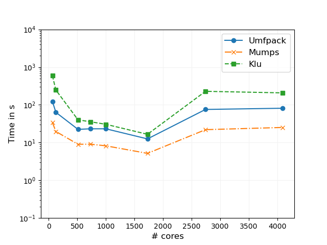
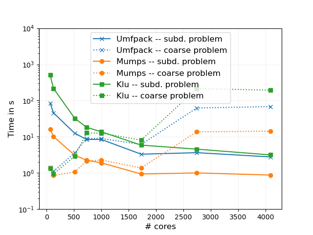
Figure 2: Strong scalability of the solver time, scaling from 64 to 4 096 cores, for the linear elasticity model problem applying the FROSch preconditioner with th GDSW coarse space (left) and the detailed timers subd. problem solve time and the coarse problem solve time (right), including the time for the factorization and the forward./backward substitution. See Table 2 for the data.

linear elasticity – GDSW

solver time

subd. problems

coarse problem

solve time

solve time

# cores

Krylov

max.

size

Amesos

Amesos2

Amesos

Amesos2

Amesos

Amesos2

it.

size $K_{i}$

$K_{0}$

MUMPS

Umfpack

KLU

MUMPS

Umfpack

KLU

MUMPS

Umfpack

KLU

64

56

86 577

932

34.04s

123.38 s

592.77 s

16.36 s

85.23 s

505.00 s

1.36 s

1.44 s

1.34 s

125

62

54 396

2 108

19.72s

63.39 s

246.96 s

10.11 s

45.80 s

217.09 s

0.85 s

1.11 s

0.94 s

512

72

21 504

10 412

9.02s

22.41 s

40.16 s

3.11 s

12.54 s

32.50 s

1.07 s

3.59 s

2.87 s

729

73

17 868

16 412

9.07s

23.21 s

35.64 s

2.25 s

8.44 s

18.27 s

2.14 s

8.95 s

12.79 s

1 000

78

14 724

20 037

8.21s

23.21 s

30.54 s

1.90 s

8.44 s

13.74 s

2.28 s

8.95 s

12.56 s

1 728

68

7 581

18 788

5.18s

12.53 s

16.58 s

0.94 s

3.30 s

5.88 s

1.38 s

6.14 s

8.10 s

2 744

86

8 700

60 090

22.02s

75.62 s

228.62 s

1.00 s

3.64 s

4.55 s

13.69 s

62.47 s

214.63 s

4 096

90

7 038

78 653

25.20s

81.41 s

207.76 s

0.87 s

2.77 s

3.15 s

14.29 s

68.19 s

194.30 s

Table 2: Strong scalability results for the linear elasticity model problem using $Q_{1}$ elements. We apply the FROSch preconditioner with the GDSW coarse space and an algebraic overlap of two elements and compare different sparse direct linear solver. The solver time is the time to build the preconditioner and to perform the Krylov iterations. The problem size is 2 738 019.

4.1 Linear Elasticity

As a first example problem, we choose the linear elasticity model problem, described in section 2.1, using $Q_{1}$ finite elements on a structured mesh with 884 736 cells such that we have 2 738 019 degrees of freedom (DOF). Since we neglect the rotations from the null space, we may expect the number of iterations to increase with an increasing number of cores. For our tests, the number of iterations increases from 56 to 90 scaling from 64 to 4 096 cores; see Table 2. Note that it has shown that the majority of the solver time is taken by the construction of the preconditioner rather than by the Krylov iterations for a smaller number of cores [17]. For this reason, the number of iterations should not influence the solver time significantly compared to the sizes of the subdomain problems within the considered range of cores.

We obtain good strong scalability results scaling from 64 to 1 728 cores for all sparse direct linear solvers with MUMPS being the fastest. Umfpack is faster than KLU, however for smaller subdomain problem sizes (obtained from 729 to 1 728 cores) the results are comparable; see Table 2 and Figure 2. Reaching 2 744 cores the solver time starts to increase instead of decreasing. The reason for that is the significant increase for the size of the coarse problem, e.g., for 1 728 dim($K_{0}$) =18 788 which compares to dim($K_{0}$) = 60 090 for 2 744 cores; see Table 2. From 2 744 cores on, the problem size relation of $K_{0}$ and max $K_{i}$ is similar to 125 cores, where the subd. problem solve time dominated the solver time. The coarse problem reaches a critical size beyond 1 728 cores, since after this point the solution of the coarse problem begins to dominate the solver time; see Figure 2. The solution on a single core is not sufficient anymore. As a next step, we could apply three-levels or/and RGDSW. We want to remark that for certain numbers of cores and numbers of elements the decomposition obtained from p4est results in structured decompositions decreasing the size of the coarse problem. The proportion of the number of elements and the number of subdomains is decisive for this phenomenon.

free-swelling problem – GDSW
solver time
	$Q_{1}Q_{1}$				$Q_{1}RT_{0}$
	avg.	Amesos		Amesos2	avg.	Amesos		Amesos2
# cores	Krylov	MUMPS	Umfpack	KLU	Krylov	MUMPS	Umfpack	KLU
64	70.9	173.24 s	536.41 s	1 587.04 s	49.7	75.35 s	238.57 s	686.13 s
125	79.8	121.68 s	362.16 s	833.82 s	56.4	53.18 s	155.20 s	352.30 s
512	103.4	71.88 s	213.51 s	250.88 s	73.7	41.18 s	122.68 s	134.44 s
729	111.0	78.86 s	258.50 s	240.84 s	78.3	54.20 s	178.32 s	200.62 s
1 000	116.3	73.49 s	241.98 s	216.39 s	81.3	53.48 s	167.36 s	154.35 s
1 728	105.1	57.20 s	190.70 s	171.00 s	76.5	38.76 s	121.18 s	128.17 s
2 744	125.1	147.99 s	599.51 s	1 068.12 s	86.8	172.00 s	646.72 s	1 547.63 s
4 096	131.9	178.61 s	755.28 s	1 428.17 s	92.3	197.48 s	836.19 s	1 428.17 s

Table 3: Strong scalability results for the free-swelling model problem. We apply the FROSch preconditioner with the GDSW coarse space and an algebraic overlap of two elements and compare different sparse direct linear solver. The solver time is the time to build the preconditioner and to perform the Krylov iterations. The problem size is 705 894 for $Q_{1}Q_{1}$ elements and 691 635 for $Q_{1}RT_{0}$ elements.

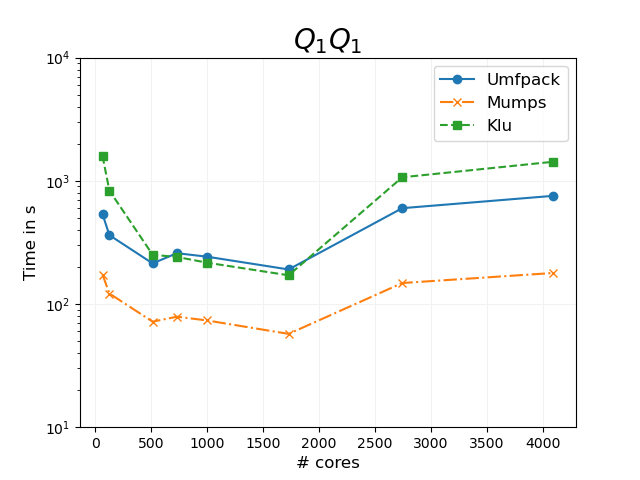
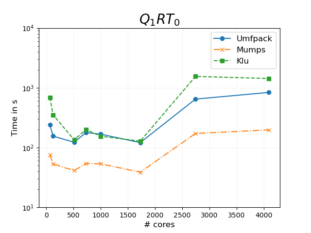
Figure 3: solver time scaling from 64 to 4 096 cores using different direct linear solvers for the subd. problems of the FROSch preconditioner with a GDSW coarse space. The preconditioner is applied the free-swelling model problem. See Table 3 for the data.

4.2 Free-swelling boundary value problem

For the model problem described in section 2.2.1, we consider a mesh with 110 592 cells. We compare two types of ansatz functions for the flux field $Q_{1}$ and $RT_{0}$, and for the deformation field, we always use $Q_{1}$ elements. For $Q_{1}Q_{1}$, we obtain 705 894 DOF and 691 635 DOF for $Q_{1}RT_{0}$. We restrict the computation to two time steps. Each requires five Newton iterations. We take the solver time over the two time steps, such that the preconditioner is applied ten times. We consider an average number of Krylov iterations (avg. Krylov) over the ten Newton steps. Since we apply FROSch fully algebraically, i.e., using the the null space of the Laplace operator for the construction of the coarse space, we cannot expect numerical scalability. Consequently, avg. Krylov increases with the number of cores; see Table 3.

Generally, the number of Krylov iterations is lower for the $Q_{1}RT_{0}$ elements, yet the increase from 64 to 4 096 cores stronger than for the $Q_{1}Q_{1}$ elements. This is in agreement with the results obtained in [17]. Further, the size of the coarse problem is much larger with increasing number of cores. For 4 096 cores, we obtain a coarse space dimension of 48 232 for $Q_{1}Q_{1}$ elements respectively 77 222 for $Q_{1}RT_{0}$ elements; see also Table 4. This indicates that the algebraic decomposition for the $Q_{1}Q_{1}$ is favorable since less interface components are obtained.

Regarding the strong scalability, we obtain similar results as for the linear elasticity model problem; compare Figures 2 and 3. For both ansatz functions, the solver time increases reaching 2 744 cores. The $Q_{1}RT_{0}$ elements are faster up to 1 728 cores. For larger number of cores the solve coarse problem time dominates the solver time. As previously discussed, the size of the coarse problem is smaller for $Q_{1}Q_{1}$ elements such that the solver time is faster for these elements employing larger numbers of cores. As for linear elasticity, the best performance of the solver framework is obtained using MUMPS. For 64 cores, MUMPS is more than 15 times faster than KLU and more than five times faster than Umfpack; see Table 3. The advantage of using MUMPS is most apparent if the size of the directly solved problem is large. From 1 728 to 4 096 the subd. problem solve time Umfpack and KLU perform similarly, e.g., considering 1 728 cores, the time to solve the $K_{i}$s is 51.02s for Umfpack and 50.89s for KLU using $Q_{1}Q_{1}$ elements; see also Table 4 and Figure 4. Generally for smaller subdomain problem sizes Umfpack and KLU are comparable.

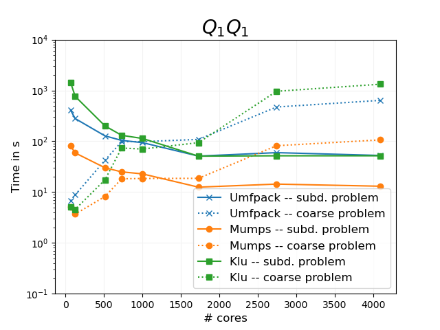
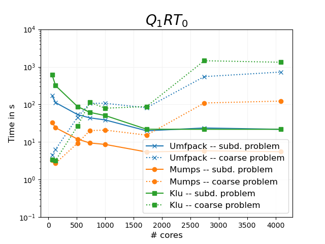
Figure 4: Time to solve the local subd. problems scaling from 64 to 4 096 cores using different direct linear. See Table 4 for the data.

free-swelling problem – GDSW
	$Q_{1}Q_{1}$				$Q_{1}RT_{0}$
subd. problem solve time
	max. size	Amesos		Amesos2	max. size	Amesos		Amesos2
	$K_{i}$	MUMPS	Umfpack	KLU	$K_{i}$	MUMPS	Umfpack	KLU
64	38 334	81.29 s	412.17 s	1 453.55 s	35 634	33.33 s	171.26 s	615.22 s
125	27 648	58.90 s	279.19 s	763.12 s	25 598	24.02 s	112.08 s	317.11 s
512	13 896	30.06 s	127.59 s	200.50 s	12 571	11.95 s	53.77 s	87.94 s
729	11 472	24.97 s	103.84 s	130.83 s	10 368	9.43 s	43.92 s	61.50 s
1000	10 452	22.79 s	93.92 s	113.40 s	9 369	8.63 s	38.68 s	50.62 s
1728	5 634	12.49 s	51.02 s	50.89 s	5 064	5.43 s	19.91 s	21.87 s
2744	7 020	14.35 s	59.66 s	51.74 s	6 209	5.84 s	23.64 s	21.81 s
4096	6 312	13.03 s	52.51 s	51.74 s	5 563	5.54 s	21.75 s	21.81 s
coarse problem solve time
	size	Amesos		Amesos2	Size	Amesos		Amesos2
	$K_{0}$	MUMPS	Umfpack	KLU	$K_{0}$	MUMPS	Umfpack	KLU
64	981	5.07 s	6.74 s	5.16 s	981	3.35 s	4.53 s	3.39 s
125	2 003	3.69 s	8.80 s	4.56 s	2 125	2.72 s	6.35 s	3.22 s
512	8 614	8.16 s	42.14 s	17.41 s	10 748	9.30 s	45.55 s	26.41 s
729	13 552	18.24 s	98.23 s	73.48 s	16 712	20.11 s	107.02 s	114.12 s
1 000	15 904	18.51 s	98.23 s	70.23 s	20 578	20.76 s	107.02 s	79.36 s
1 728	18 788	18.62 s	108.68 s	93.77 s	18 788	15.24 s	81.61 s	87.93 s
2 744	37 229	81.63 s	471.65 s	961.46 s	57 308	109.34 s	550.39 s	1 456.04 s
4 096	48 232	106.39 s	637.60 s	1 325.53 s	77 222	122.81 s	727.94 s	1 325.53 s

Table 4: Strong scalability for the subd. problem solve time and the coarse problem solve time using different sparse direct linear solvers. The time includes the factorization of problem and the forward./backw. substitution during the Krylov iterations. For the whole solver time see Table 3

Although MUMPS is much faster than Umfpack and KLU the scalability is not extended solely by this choice of the direct linear solver.

4.3 Mechanically induced diffusion problem

The results for the mechanically induced diffusion problem, introduced in section 2.2.2, confirm the results obtained for the free-swelling boundary value problem. Here, we also restrict the computation to two timesteps each solved with five Newton iterations. The more complex boundary conditions result in higher numbers of Krylov iterations. As for the other model problems, the number os iterations increases with an increasing number of cores.

mechanically-induced diffusion problem – GDSW
solver time
	$Q_{1}Q_{1}$				$Q_{1}RT_{0}$
	avg.	Amesos		Amesos2	Avg.	Amesos		Amesos2
# cores	Krylov	MUMPS	Umfpack	KLU	Krylov	MUMPS	Umfpack	KLU
64	115.8	214.14 s	739.30 s	1 654.99 s	119.9	113.30 s	432.78 s	753.36 s
125	130.0	154.23 s	500.88 s	887.11 s	137.2	85.14 s	300.36 s	399.83 s
512	177.2	100.06 s	323.04 s	292.94 s	180.3	74.06 s	265.61 s	183.75 s
729	186.4	112.14 s	390.50 s	288.87 s	192.3	102.14 s	395.56 s	260.95 s
1 000	196.4	107.12 s	374.02 s	262.23 s	205.4	106.15 s	386.94 s	224.96 s
1 728	210.6	97.71 s	356.62 s	226.93 s	219.5	88.08 s	320.87 s	192.73 s
2 744	224.4	241.59 s	1 008.08 s	1 212.64 s	235.6	362.65 s	1 561.48 s	1 846.48 s
4 096	239.1	295.22 s	1 283.16 s	1 606.95 s	249.0	422.36 s	2 027.79 s	2 372.35 s

Table 5: Strong scalability results for the mechanically-induced diffusion model problem. We apply the FROSch preconditioner with the GDSW coarse space and an algebraic overlap of two elements and compare different sparse direct linear solver. The solver time is the time to build the preconditioner and to perform the Krylov iterations. The problem size is 705 894 for $Q_{1}Q_{1}$ elements and 691 635 for $Q_{1}RT_{0}$ elements.

Yet, the change of boundary conditions does not affect the domain decomposition, such that the sizes for the subdomain problems $K_{i}$ and the coarse problem $K_{0}$ are equal. Therefore, the strong scaling behavior is similar to the free-swelling problem; see Table 5. Consequently, for these tests, the solver time obtained using MUMPS is the fastest as well. The results comparing Umfpack and KLU for this model problem are remarkable. From 512 to 1 728 cores the solver time using KLU is slightly faster than Umfpack, although it has been slower for the free-swelling model problem. The time to solve the subdomain problems again dominates solver time scaling from 64 to 1 000 cores; see Tables 5 and 6 and Figures 5 and 6.

mechanically induced diffusion problem – GDSW
	$Q_{1}Q_{1}$				$Q_{1}RT_{0}$
subd. problem solve time
	max. size	Amesos		Amesos2	max. size	Amesos		Amesos2
	$K_{i}$	MUMPS	Umfpack	KLU	$K_{i}$	MUMPS	Umfpack	KLU
64	38 334	115.89 s	609.33 s	1 515.37 s	35 634	61.56 s	351.75 s	673.00 s
125	27 648	85.54 s	409.80 s	809.69 s	25 598	47.02 s	239.01 s	356.35 s
512	13 896	46.94 s	207.11 s	229.25 s	12 571	25.06 s	122.50 s	112.68 s
729	11 472	38.56 s	166.92 s	152.12 s	10 368	20.03 s	100.85 s	81.18 s
1 000	10 452	35.56 s	152.18 s	131.74 s	9 369	18.88 s	92.55 s	69.41 s
1 728	5 634	22.80 s	90.63 s	65.87 s	5 064	13.30 s	53.54 s	34.12 s
2 744	7 020	23.92 s	101.89 s	65.43 s	6 209	13.75 s	62.04 s	34.43 s
4 096	6 312	21.98 s	89.07 s	65.43 s	5 563	13.01 s	56.25 s	34.43 s
coarse problem solve time
	max. size	Amesos		Amesos2	max. size	Amesos		Amesos2
	$K_{i}$	MUMPS	Umfpack	KLU	$K_{i}$	MUMPS	Umfpack	KLU
64	981	5.32 s	7.92 s	5.42 s	981	4.36 s	7.18 s	4.43 s
125	2 003	4.25 s	12.21 s	5.34 s	2 125	4.06 s	13.04 s	5.08 s
512	8 614	11.64 s	68.46 s	22.99 s	10 748	16.23 s	103.86 s	38.81 s
729	13 552	25.86 s	167.40 s	87.50 s	16 712	35.08 s	239.38 s	132.98 s
1 000	15 904	26.73 s	167.40 s	85.64 s	20 578	38.30 s	239.38 s	107.88 s
1 728	18 788	30.67 s	206.60 s	116.33 s	18 788	31.65 s	218.03 s	117.71 s
2 744	37 229	119.86 s	788.58 s	1 059.76 s	57 308	204.04 s	1 315.37 s	1 633.51 s
4 096	48 232	156.47 s	1 076.23 s	1 432.02 s	77 222	233.64 s	1 748.85 s	2 130.84 s

Table 6: Strong scalability for the subd. problem solve time and the coarse problem solve time using different sparse direct linear solvers. The time includes the factorization of problem and the forward./backw. substitution during the Krylov iterations. For the whole solver time see Table 5

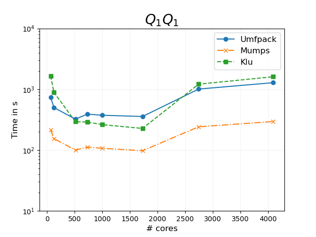
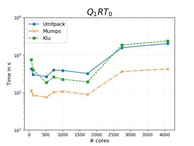
Figure 5: Solver time scaling from 64 to 4 096 cores using different direct linear solvers for the subd. problems of the FROSch preconditioner with a GDSW coarse space. The preconditioner is applied the mechanically induced diffusion model problem. See Table 5 for the data.

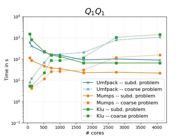
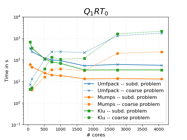
Figure 6: Time to solve the local subd. problems scaling from 64 to 4 096 cores using different direct linear. See Table 6 for the data.

5 Conclusion

In our tests, we were able to reduce the solver time by over 80% with the choice of the sparse solver. We should therefore take particular interest in the choice of the solver using FROSch. For the considered model problems, we recommend using MUMPS since it performed the best. We expect a good performance of MUMPS for other model problems as well.

For the range of problems considered here, we did not face any memory issues with the direct solvers compared, and we did not specifically examine the memory usage. However, we expect differences in the range of possible subdomain and coarse problem sizes due to different memory demands of the different solvers.

References

- [1] Reference documentation for deal.II version 9.3.0 - the step-8 tutorial program., 2021.
- [2] Trilinos public git repository. Web, 2021.
- [3] P. Amestoy, A. Buttari, I. Duff, A. Guermouche, J.-Y. L’Excellent, and B. Uçar. Mumps. In D. Padua, editor, Encyclopedia of Parallel Computing, pages 1232–1238. Springer US, Boston, MA, 2011.
- [4] W. Bangerth, C. Burstedde, T. Heister, and M. Kronbichler. Algorithms and data structures for massively parallel generic adaptive finite element codes. ACM Trans Math Softw, 38(2):1–28, 2011.
- [5] L. Böger, A. Nateghi, and C. Miehe. A minimization principle for deformation-diffusion processes in polymeric hydrogels: Constitutive modeling and FE implementation. Int J Solids Struct, 121:257–274, 2017.
- [6] C. Burstedde, L. C. Wilcox, and O. Ghattas. p4est: Scalable algorithms for parallel adaptive mesh refinement on forests of octrees. SIAM J Sci Comput, 33(3):1103–1133, 2011.
- [7] T. A. Davis and I. S. Duff. A combined unifrontal/multifrontal method for unsymmetric sparse matrices. ACM Trans Math Softw, 25(1):1–20, 1999.
- [8] C. R. Dohrmann, A. Klawonn, and O. B. Widlund. Domain decomposition for less regular subdomains: Overlapping Schwarz in two dimensions. SIAM J Numer Anal, 46(4):2153–2168, 2008.
- [9] C. R. Dohrmann, A. Klawonn, and O. B. Widlund. A family of energy minimizing coarse spaces for overlapping Schwarz preconditioners. In Domain decomposition methods in science and engineering XVII, volume 60 of LNCSE. Springer, 2008.
- [10] C. R. Dohrmann and O. B. Widlund. On the design of small coarse spaces for domain decomposition algorithms. SIAM J Sci Comput, 39(4):A1466–A1488, 2017.
- [11] A. Heinlein, C. Hochmuth, and A. Klawonn. Fully algebraic two-level overlapping Schwarz preconditioners for elasticity problems. In F. Vermolen and C. Vuik, editors, Numerical Mathematics and Advanced Applications ENUMATH 2019, pages 531–539, Cham, 2021. Springer International Publishing.
- [12] A. Heinlein, A. Klawonn, S. Rajamanickam, and O. Rheinbach. FROSch: A fast and robust overlapping Schwarz domain decomposition preconditioner based on Xpetra in Trilinos. In R. Haynes, S. MacLachlan, X.-C. Cai, L. Halpern, H. H. Kim, A. Klawonn, and O. Widlund, editors, Domain Decomposition Methods in Science and Engineering XXV, pages 176–184, Cham, 2020. Springer.
- [13] A. Heinlein, A. Klawonn, and O. Rheinbach. A parallel implementation of a two-level overlapping Schwarz method with energy-minimizing coarse space based on Trilinos. SIAM J Sci Comput, 38(6):C713–C747, 2016.
- [14] A. Heinlein, O. Rheinbach, and F. Röver. Parallel scalability of three-level FROSch preconditioners to 220 000 cores using the theta supercomputer. SIAM J Sci Comput, 45(3):S173–S198, 2023.
- [15] A. Heinlein, O. Rheinbach, F. Röver, S. Sandfeld, and D. Steinberger. Applying the FROSch overlapping Schwarz preconditioner to dislocation mechanics in deal.ii. PAMM, 19(1):e201900337, 2019.
- [16] Jülich Supercomputing Centre. JUWELS Cluster and Booster: Exascale Pathfinder with Modular Supercomputing Architecture at Juelich Supercomputing Centre. Journal of large-scale research facilities, 7(A138), 2021.
- [17] B. Kiefer, S. Prüger, O. Rheinbach, and F. Röver. Monolithic parallel overlapping Schwarz methods in fully-coupled nonlinear chemo-mechanics problems. Comput Mech, 71(4):765–788, 2023.
- [18] A. McBride, A. Javili, P. Steinmann, and B. D. Reddy. A finite element implementation of surface elasticity at finite strains using the deal.II library. arXiv:1506.01361 [physics], June 2015.
- [19] A. Toselli and O. Widlund. Domain decomposition methods—algorithms and theory, volume 34 of Springer Series in Computational Mathematics. Springer-Verlag, Berlin, 2005.