Meta-Learning With Hierarchical Models Based on Similarity of Causal Mechanisms

Abstract

In this work the goal is to generalise to new data in a non-iid setting where datasets from related tasks are observed, each generated by a different causal mechanism, and the test dataset comes from the same task distribution. This setup is motivated by personalised medicine, where a patient is a task and complex diseases are heterogeneous across patients in cause and progression. The difficulty is that there usually is not enough data in one task to identify the causal mechanism, and unless the mechanisms are the same, pooling data across tasks, which meta-learning does one way or the other, may lead to worse predictors when the test setting may be uncontrollably different. In this paper we introduce to meta-learning, formulated as Bayesian hierarchical modelling, a proxy measure of similarity of the causal mechanisms of tasks, by learning a suitable embedding of the tasks from the whole data set. This embedding is used as auxiliary data for assessing which tasks should be pooled in the hierarchical model. We show that such pooling improves predictions in three health-related case studies, and by sensitivity analyses on simulated data that the method aids generalisability by utilising interventional data to identify tasks with similar causal mechanisms for pooling, even in limited data settings.

1 Introduction

Given a dataset of related tasks, how can we train a machine learning model that performs well on new data? This is the fundamental problem of generalisation in machine learning. In this work we study generalisation for supervised learning tasks (i.e., learning to predict outputs $\bm{y}$ from inputs $\bm{x}$) in a non-iid setting where datasets consist of related supervised learning tasks that may be generated by different causal mechanisms. This setup is motivated by real-world settings, where causally heterogeneous datasets arising from different populations, experiment regimes and sampling methods create challenges such as confounding and cross-population biases (Bareinboim and Pearl, 2016). These issues disrupt predictive algorithms applied to causally heterogeneous datasets.

Causally heterogeneous datasets are common in healthcare, epidemiology and economics, for example, where data is rarely collected in an idealised iid setting. The causal mechanisms are typically unknown and cannot be accurately established from the data (e.g., due to a limited number of data samples or lack of the appropriate data needed for causal identifiability), so predictive models applied to these datasets may not be explicitly utilising causal properties of the data that can aid with generalisability. For example, precision medicine applications require accurate models for individual patients. This is challenging for complex diseases such as type 2 diabetes and Alzheimer’s disease, where differences in patient outcomes are driven by different underlying biological processes of disease (Nair et al., 2022; Scheltens et al., 2016). Predictive models can pool data from similar patients (e.g., based on similar health outcomes or other patient attributes) to improve individual-level performance (Suresh et al., 2018; Alaa et al., 2017), but it is challenging to identify similar patients based on the true causal mechanisms of disease.

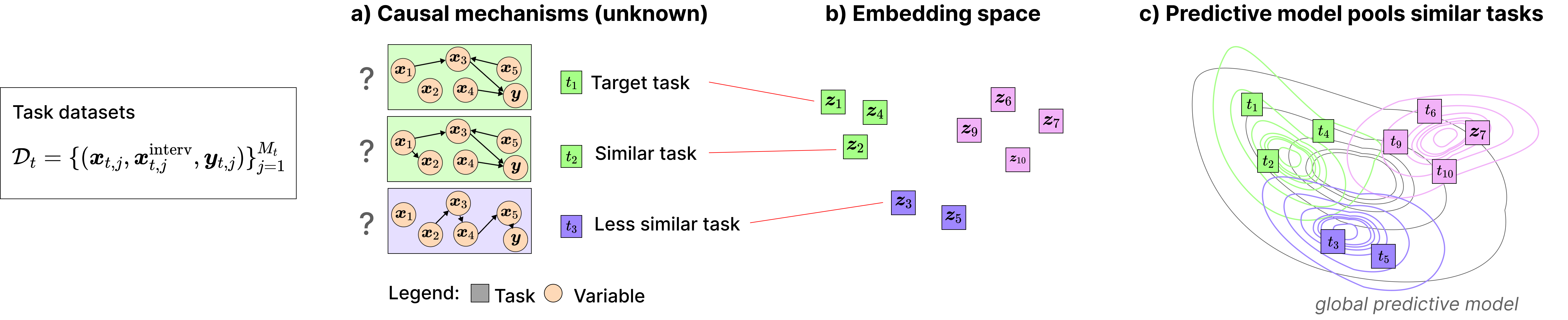
Figure 1: (a) Each task is assumed to have been generated by a causal model, but these models are unknown and infeasible to infer for each task from the task-specific data alone; (b) Groups of tasks with similar causal models are approximated by embedding the tasks in a latent space that generates structural causal models; (c) The similarity of the causal mechanisms can be used in grouping tasks in a hierarchical predictive model, to improve task-level predictive performance and generalisation to new tasks.

In this work we relate this to the more general machine learning problem of learning from multiple related tasks (from a common task environment), where some aspects of the data are common across all tasks (global properties), but other aspects are unique to a specific task (local properties). This problem has been examined in learning paradigms such as hierarchical Bayesian models, meta-learning and multi-task learning (Caruana, 1997; Gelman and Hill, 2006; Hospedales et al., 2021). The meta-learning framework, in particular, aims to ”learn how to learn” a model for a new task with only a limited amount of data (Thrun and Pratt, 2012; Wang et al., 2020), and has been successfully applied to non-iid datasets in healthcare and other domains (Rafiei et al., 2023). Extensions to the popular approach of model-agnostic meta-learning (MAML) (Finn et al., 2017) show that it is beneficial to consider the underlying similarity structure between tasks (e.g., similar tasks in the feature space, model parameter space, or meta-knowledge space) (Zhou et al., 2021; Yao et al., 2019a, b). However, existing meta-learning methods do not consider the causal similarity structure of the tasks, and therefore may fail to learn important information that can aid with generalisation.

To address this gap, we consider a problem setup of multiple, related supervised prediction tasks sampled from a causally heterogeneous task environment, and we study the meta-learning problem of generalisation to new tasks from the same task environment, assuming there are few labelled samples for each new task. In a causally heterogeneous task environment each task may have been generated by a different causal mechanism. This setup is motivated by personalised medicine, where a patient is a task and complex diseases are heterogeneous across patients in cause and progression. As is typically the case, our problem setting assumes that task-specific data is not sufficient for identifying the causal mechanisms. However, given a large enough set of tasks, even a simple model of causal mechanisms may be able to give useful information about the mechanisms. For learning that model, we assume that the data has been observed under various interventional settings which induce some information about the causal mechanisms, even indirectly. The problem setting and our approach is visualised in Fig. 1.

The main contributions of this work are as follows:

• We formulate the problem of meta-learning predictive models in causally heterogeneous task environments (assuming unknown causal models) and propose a method for this problem, formulated as Bayesian hierarchical modelling, that learns how to pool data across tasks with similar causal mechanisms.

• We demonstrate on simulated data and three health-related applications that the method improves generalisability in causally heterogeneous task environments, even in settings with limited data for tasks.

The code for the method and experiments presented in this work is publicly available at https://github.com/sophiewharrie/meta-learning-hierarchical-model-similar-causal-mechanisms.

2 Related Work

2.1 OOD Generalisation and Meta-Learning

A variety of techniques have been developed to improve the performance of predictive models on out-of-distribution (OOD) data (data that is different from the training data) for various problem settings, including meta-learning, multi-task learning, domain adaptation, and domain generalisation. Our work uses the meta-learning problem setting, which aims to “learn how to learn” by training a model on multiple related tasks and then using this experience to adapt quickly to new tasks with few labelled samples (see, e.g., Hospedales et al. (2021) for a review).

We formulate the meta-learning problem in terms of Bayesian hierarchical modelling, which relates to previous Bayesian meta-learning methods (Grant et al., 2019; Gordon et al., 2019; Ravi and Beatson, 2018; Amit and Meir, 2018). Recent extensions to general meta-learning methods show that task similarity can be exploited to further improve performance, e.g., in the feature space, model parameter space, or meta-knowledge space (Zhou et al., 2021; Yao et al., 2019a, b). These methods use the similar tasks to tailor the parameter initialisation of a meta-learning algorithm, whereas in a Bayesian meta-learning context, our work is better understood as using similar tasks to meta-learn a prior distribution for the predictive models of new tasks. Our method extends previous work on task-similarity in meta-learning by incorporating causal task similarity into the Bayesian meta-learning framework, to address the problem of meta-learning in causally heterogeneous task environments.

There is also a tangential link to Bayesian switching linear dynamical systems (Linderman et al., 2017), which can be seen as hierarchical models in the special case of dynamical systems, and where the dynamical system models are, in a sense, models of the systems’ causal mechanisms.

2.2 Causality-Inspired Approaches for OOD Generalisation

Utilising ideas from causal inference to improve the generalisation of predictive models is an active topic of research. Peters et al. (2016) introduced invariant causal prediction for selecting the set of features which are causal predictors of a target variable. Furthermore, several graph pruning approaches have been proposed for the domain adaptation problem setting, based on the assumption of an underlying invariant causal mechanism that is persistent across environments (Rojas-Carulla et al., 2018; Magliacane et al., 2018), while graph surgery aims to create estimators that are invariant across environments (Subbaswamy et al., 2019; Subbaswamy and Saria, 2018). Like our method, the objective of these approaches is not causal reasoning, but rather to improve predictive models by reducing the influence of data without a direct causal relationship to the outcomes being predicted. These methods make assumptions about available data that are incompatible to our setup, because they have been developed for different settings, and cannot be straightforwardly included in our setup. The principle of invariant causal prediction could in principle be used also in our method, within each task or task cluster, given suitable data. However, based on preliminary experiments, a straightforward implementation did not improve results over the embedding method described in Sec. 4, and we leave more refined combinations as future work.

3 Preliminaries

3.1 Problem specification for meta-learning in a causally heterogeneous task environment

We formulate the problem setup studied in this work as follows. Each task $t$ is sampled from a task environment defined by a task distribution $t\sim p(\mathcal{T})$ (standard setup in inductive bias, Baxter (2000)). In this work we are interested in causally heterogeneous task environments, where each task is generated by a causal model (one causal model per task) and the causal models differ between tasks. We assume it is infeasible to infer the true causal model for each task from the task data alone, due to limited data, which is why we develop meta-learning techniques for predictive modelling (i.e., as opposed to directly using a causal model such as an SCM for the purpose of predictive modelling). To aid with identifying tasks with similar causal models, we utilise the idea that a causal model may become identifiable when the data is observed under different experiment conditions (“environments”) (Tian and Pearl, 2001; Hauser and Bühlmann, 2012; Hyttinen et al., 2012). Specifically, we assume that the data is observed under different interventional settings $\mathcal{I}\subseteq\{X_{1},...,X_{K}\}$, and, for simplicity, that these settings are the same for all tasks.

Each task $t$ has $M_{t}$ labelled samples $\mathcal{D}_{t}=\{(\bm{x}_{t,j},\bm{x}^{\text{interv}}_{t,j},\bm{y}_{t,j})\}_{j=1}^{M_{t}}$ from a task-specific data distribution $p(\mathcal{D}\mid\mathcal{T}=t)$, where $\bm{x}_{t,j}\in\mathcal{X}\subseteq\mathbb{R}^{K}$ contains the same $K$ variables for all tasks and the goal is to learn how to predict outputs $\bm{y}_{t}$ from inputs $\bm{x}_{t}$ for each task. Known (hard) intervention targets are indicated by a binary mask $\bm{x}^{\text{interv}}_{t,j}\in\{0,1\}^{K}$ for each data sample.

Meta-learners aim to learn some knowledge from a training set of $N$ tasks that will facilitate the learning of new tasks (from the same task environment) with few labelled samples. To achieve this, the task data $\mathcal{D}_{t}$ is typically split into support $\mathcal{D}_{t}^{(s)}$ and query $\mathcal{D}_{t}^{(q)}$ sets. The support set is used to adapt the meta-learner to the task at hand, and the query set is used to update the meta-learner’s ability to generalise to new data from the same task. In this work we evaluate performance in terms of generalisation to new tasks from the same task environment, assuming there are few labelled observations available for each new task, i.e., for a new task $s$, the meta-learner is adapted using the support samples $\mathcal{D}_{s}^{(s)}$, and evaluated using the query samples $\mathcal{D}_{s}^{(q)}$.

3.2 Causal models for tasks

In this paper we utilise the framework of structural causal models (SCMs) (Pearl, 2009) as a simplified mathematical model of the causal mechanisms. An SCM is described by a collection of structural equations $V_{u}:=f_{u}(\operatorname{\textbf{PA}}_{u}^{\mathcal{G}},\epsilon_{u};\bm{\Theta}_{u})$ for $u=1,...,K+1$, where $\mathcal{G}=(\bm{V},\bm{E})$ is a directed acyclic graph (DAG) consisting of $K+1$ vertices $\bm{V}=\{X_{1},...,X_{K},Y\}$ and the edge set $\bm{E}\subseteq\bm{V}^{2}$, $\operatorname{\textbf{PA}}_{u}^{\mathcal{G}}$ are parent vertices of $V_{u}$, $\bm{\Theta}_{u}$ are parameters of the structural equation, and $\epsilon_{u}$ is exogenous noise. For a task $t$ with causal DAG $\mathcal{G}_{t}$ and data observed under interventional setting $\mathcal{I}$, the interventional Markovian factorisation expresses the joint distribution over the data $(X_{1},...,X_{K},Y)$ as

$$p(\mathcal{D}\mid\mathcal{T}=t;\operatorname{do}{\{V_{u}=W_{u}\}_{u\in\mathcal{I}}})=\prod_{u\notin\mathcal{I}}p(V_{u}\mid\operatorname{\textbf{PA}}_{u}^{\mathcal{G}_{t}})\prod_{u\in\mathcal{I}}p(V_{u}),$$ (1)

where $\operatorname{do}{\{\cdot\}}$ is the do-operator (Pearl, 2009).

3.3 Learning from related tasks using hierarchical models

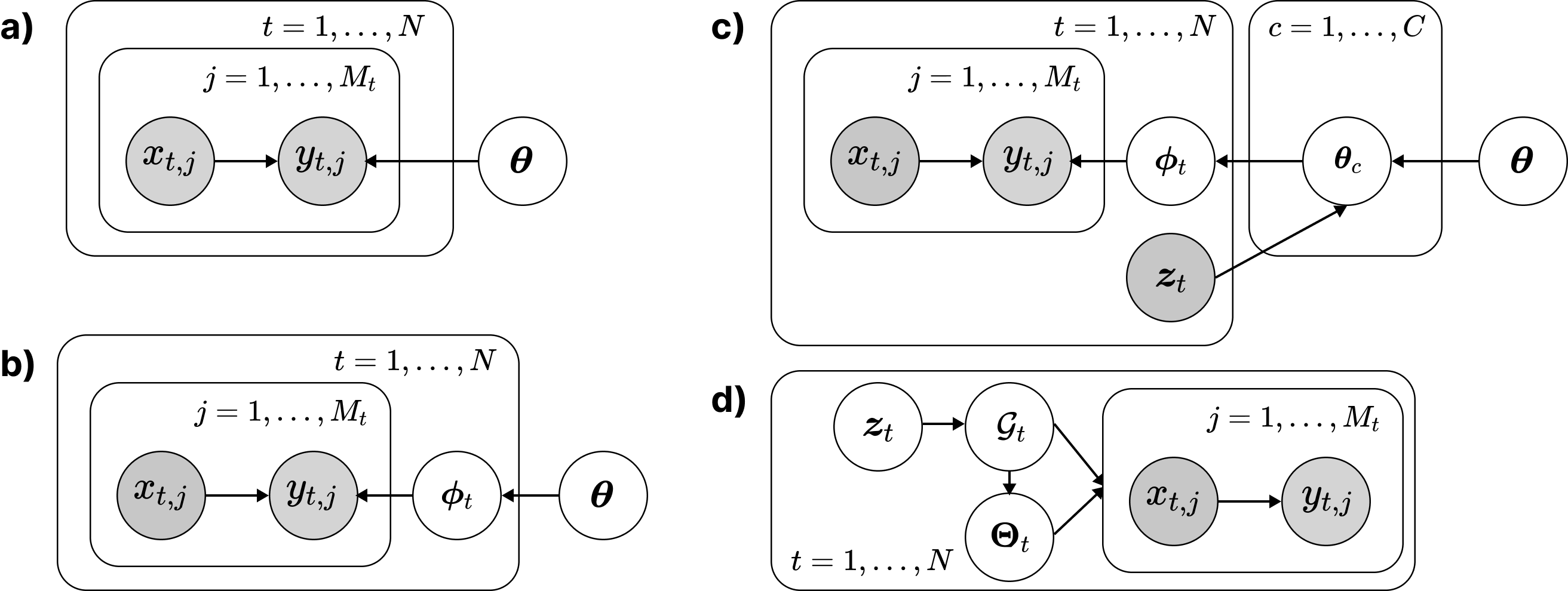
Figure 2: (a) Global model with parameters $\bm{\theta}$ shared across all $N$ tasks; (b) Hierarchical model with global parameters $\bm{\theta}$ and task-specific parameters $\bm{\phi_{t}}$ for each task $t=1,...,N$; (c) Our approach, which introduces parameters $\bm{\theta}_{c}$ for pooling across $c=1,...,C$ groups of causally similar tasks and side data $\bm{z}_{t}$ for embedding the inferred causal mechanisms of the tasks; (d) The side data is generated from structural causal models with parameters $(\mathcal{G}_{t},\bm{\Theta}_{t})$, learned from all available data.

We utilise hierarchical Bayesian models (HBMs) as the basis of our meta-learning method. A basic HBM consists of global parameters $\bm{\theta}$ that act to pool information across multiple tasks and task-specific parameters $\bm{\phi}_{t}$ that allow for variation between tasks. HBMs can be used to formulate Bayesian meta-learning methods, where the aim is to meta-learn a global prior $p(\bm{\theta})$ from the training data that is suitable for deriving posterior distributions of the local parameters for new tasks (Grant et al., 2019; Gordon et al., 2019; Fortuin, 2022). For prior distributions $p(\bm{\phi}_{t}\mid\bm{\theta}),p(\bm{\theta})$, the posterior distribution of the local model $p(\bm{\phi}_{t}\mid\mathcal{D}_{t}^{(s)},\bm{\theta})$ is inferred and the posterior predictive distribution for the unseen data is computed as

$$\textit{p}(\bm{y}_{t}^{(q)}\mid\bm{x}_{t}^{(q)},\bm{\theta})=\int p(\bm{y}_{t}^{(q)}\mid\bm{x}_{t}^{(q)},\bm{\phi}_{t},\bm{\theta})p(\bm{\phi}_{t}\mid\mathcal{D}_{t}^{(s)},\bm{\theta})d\bm{\phi}_{t}.$$ (2)

Fig. 2 illustrates the difference between a non-hierarchical model (2a) and an HBM (2b). As described in Sec. 4.1, we build on this approach to meta-learn from causally similar tasks.

4 Our Method

We present a method for the problem setup described in Sec. 3.1, based on the idea that task-level performance can be improved by pooling data from related tasks. We introduce to meta-learning, formulated as Bayesian hierarchical modelling, a proxy measure of similarity of the causal mechanisms of tasks, by learning a suitable embedding of the tasks from the whole data set. This embedding (generated by the model shown in Fig. 2d) is used as auxiliary data for assessing which tasks should be pooled in the hierarchical model (Fig. 2c). Details of the hierarchical model and embedding are described in Sec. 4.1 and 4.2, respectively.

4.1 Learning from causally similar tasks

We extend the hierarchical model (2) to also pool data across causally similar tasks. Here we make the simplifying approximation that the tasks come in clusters having similar causal mechanisms; this approximation is reasonable because many real world datasets exhibit a clustering structure, e.g., subtypes of disease in medical datasets (Turner et al., 2015; Seymour et al., 2019). Based on this idea, we add an extra level in the hierarchical model with parameters $\bm{\theta}_{c}$ for $c=1...,C$ groups of causally related tasks (illustrated in Fig. 2c). The posterior distribution over the model parameters becomes

$$p(\bm{\theta},\bm{\theta}_{1},...,\bm{\theta}_{C},\bm{\phi}_{1},...,\bm{\phi}_{N}\mid\mathcal{D}_{1},...,\mathcal{D}_{N})=\textit{p}(\bm{\theta}\mid\mathcal{D}_{1},...,\mathcal{D}_{N})\prod_{c=1}^{C}p(\bm{\theta}_{c}\mid\bm{\theta},\mathcal{D}_{1},...,\mathcal{D}_{N_{c}})\prod_{t=1}^{N}p(\bm{\phi_{t}}\mid\bm{\theta}_{c_{t}},\mathcal{D}_{t}).$$ (3)

We would like to emphasise that in principle, our approach does not rely on the specific assumption that the data can be partitioned into $C$ groups of causally similar tasks; alternatively, there could be a similarity kernel or latent-variable model connecting the tasks. We use variational inference to estimate (3), with details of the formulation of this as a meta-learning optimisation problem given in Sec. 5.

4.2 Identifying causally similar tasks

To learn from tasks with similar causal mechanisms, we first need to define a measure of causal similarity for tasks. In experiments, we utilise a distance $d(t_{1},t_{2}):=d((\mathcal{G}_{t_{1}},\bm{\Theta}_{t_{1}}),(\mathcal{G}_{t_{2}},\bm{\Theta}_{t_{2}}))$, where a small distance indicates that the tasks $t_{1},t_{2}$ have similar causal models. If the causal models for the tasks were known, then the Structural Hamming Distance (SHD) (Acid and de Campos, 2003) or interventional distances (Peters and Bühlmann, 2015; Peyrard and West, 2021) could be used. However, since we are dealing with unknown causal models, determining causally similar tasks relies on identifiability of the causal models (or at least partial identifiability to the extent that the distinguishing factors of the causal models of different tasks can be determined). Assuming there is not sufficient data in each task, we cannot infer the causal model $(\mathcal{G}_{t},\bm{\Theta}_{t})$ from only the task data. Instead, we leverage the idea of “foundation models” and learn from the larger set of $N$ training tasks a generative model of causal models, and use it to embed each task in a latent space $\bm{z}$, where distances $d(t_{1},t_{2})\approx d(\bm{z}_{t_{1}},\bm{z}_{t_{2}})$ serve as proxies for causal similarity.

For learning the embedding, we utilise recent developments in differentiable causal discovery techniques (Lorch et al., 2021; Brouillard et al., 2020). We follow prior work (Lorch et al., 2021) in formulating $\bm{z}_{t}$ to model the generative process of a structural causal model. Specifically, $\bm{z}_{t}=[\bm{u}_{t},\bm{v}_{t}]$ is defined in terms of $\bm{u}_{t},\bm{v}_{t}\in\mathbb{R}^{\rho\times(K+1)}$ (where $\rho$ is the dimension of a latent space), and the adjacency matrix $A_{t}\in\{0,1\}^{(K+1)\times(K+1)}$ of the causal DAG $\mathcal{G}_{t}$ is encoded by a bilinear generative model:

$$A_{t}(\bm{z}_{t})_{ij}:=p_{\alpha}(a_{ij}=1\mid\bm{u}_{t,i},\bm{v}_{t,j})=\begin{cases}\sigma_{\alpha}(\bm{u}_{t,i}^{T}\bm{v}_{t,j})&\text{if }i\neq j\\ 0&\text{if }i=j,\end{cases}$$ (4)

where $\sigma_{\alpha}$ is the sigmoid function with inverse temperature $\alpha$. The prior $p(\bm{z}_{t})$ encourages valid DAGs by penalising cyclicity:

$$p(\bm{z}_{t})\propto\exp{\big{(}-\beta\mathbb{E}_{p(A_{t}\mid\bm{z}_{t})}[h(A_{t})]\big{)}}\prod_{ij}\mathcal{N}(z_{t,ij};0,\sigma^{2}_{z}),$$ (5)

where $\beta$ controls how strongly the acyclicity is enforced and $h(A_{t}):=\operatorname{tr}{[(\bm{I}+\frac{1}{K+1}A_{t})^{(K+1)}]}-K-1$ is a DAG constraint function where $h(A_{t})=0$ if and only if $A_{t}$ does not have any cycles (Yu et al., 2019). In experiments we consider both linear and non-linear Gaussian SCMs, and Erdős-Rényi and scale-free graph priors (as an additional term in (5)). Further details are given in Appendix A.3. The inference procedure for inferring $p(\bm{z}_{t}\mid\mathcal{D}_{t})$ for each task is described in Sec. 5.

5 Application for Bayesian Neural Networks

We propose an algorithm for implementing our method for Bayesian neural networks (BNNs), which is used in experiments in this paper. This consists of a meta-learning procedure for the $N$ training tasks, as well as a procedure for adapting the meta-learner to new tasks (given few labelled observations). These are described in Algorithm 1 and Algorithm 2 (in Appendix A.1), respectively, and summarised below.

5.1 Meta-learning procedure

A variational inference approach is used to estimate (3) using a family of variational distributions:

$$q(\bm{\theta},\bm{\theta}_{1},...,\bm{\theta}_{C},\bm{\phi}_{1},...,\bm{\phi}_{N})=q_{\bm{\psi}}(\bm{\theta})\prod_{c=1}^{C}q_{\bm{\psi}_{c}}(\bm{\theta}_{c})\prod_{t=1}^{N}q_{\bm{\gamma}_{t}}(\bm{\phi}_{t}),$$ (6)

where $\bm{\psi},\bm{\psi}_{1},...,\bm{\psi}_{C},\bm{\gamma}_{1},...,\bm{\gamma}_{N}$ are unknown neural network parameters. The optimisation objective for this problem is

$$\underset{\bm{\psi},\bm{\psi}_{1},...,\bm{\psi}_{C},\bm{\gamma}_{1},...,\bm{\gamma}_{N}}{\operatorname{argmin}}\mathbb{E}_{q_{\bm{\psi}}}\big{[}\sum_{c=1}^{C}\mathbb{E}_{q_{\bm{\psi}_{c}}}\big{[}\sum_{t=1}^{N_{c}}\mathcal{L}_{\mathcal{D}_{t}^{(s)}}(\bm{\gamma}_{t})\big{]}+D_{KL}(q_{\bm{\psi}_{c}}(\bm{\theta}_{c})\;\|\;p(\bm{\theta}_{c}\mid\bm{\theta}))\big{]}+D_{KL}(q_{\bm{\psi}}(\bm{\theta})\;\|\;p(\bm{\theta})),$$ (7)

where the part of the optimisation objective corresponding to the task data is denoted by

$$\mathcal{L}_{\mathcal{D}_{t}}(\bm{\gamma}_{t})=D_{KL}(q_{\bm{\gamma}_{t}}(\bm{\phi}_{t}\mid\mathcal{D}_{t})\;\|\;p(\bm{\phi}_{t}\mid\bm{\theta_{c}}))-\mathbb{E}_{q_{\bm{\gamma}_{t}}}[\log p(\mathcal{D}_{t}\mid\bm{\phi}_{t})].$$ (8)

Further details on the derivation of the optimisation objective are given in Appendix A.2. The global parameters use a sparsity-inducing Gaussian scale mixture prior,

$$p(\bm{\theta})=\pi_{\theta}N(\bm{\theta};\bm{0},\sigma_{\theta,1}^{2}\bm{I})+(1-\pi_{\theta})N(\bm{\theta};\bm{0},\sigma_{\theta,2}^{2}\bm{I})$$ (9)

while the priors for the group and local parameters are adapted during training:

$$p(\bm{\theta}_{c}\mid\bm{\theta})=N(\bm{\theta}_{c};\bm{\mu}_{\bm{\theta}},\bm{\sigma}^{2}_{\bm{\theta}}\bm{I}),p(\bm{\phi}_{t}\mid\bm{\theta}_{c},\bm{\theta})=N(\bm{\phi}_{t};\bm{\mu}_{\bm{\theta}_{c}},\bm{\sigma}^{2}_{\bm{\theta}_{c}}\bm{I}).$$ (10)

We use a meta-learning approach similar to the amortised variational inference method proposed by Ravi and Beatson (2018) (but extended to an additional hierarchical level), which reduces memory requirements by computing local variational parameters on the fly for each task.

For forming the task clusters, we first learn a task embedding given all available data, using the method described in Sec. 4.2. The embeddings $\bm{z}_{t}$ of each task are then used as auxiliary data for each task $t$. In experiments we use the Stein variational gradient descent (SVGD) algorithm implemented by Lorch et al. (2021) for this generative model, which supports inference from interventional data via the interventional log (marginal) likelihood (i.e, see (1)). A distance matrix $\tilde{D}\in\mathbb{R}^{N\times N}$ is constructed by calculating $d(t_{i},t_{j})\approx d(\tilde{\bm{z}}_{t_{i}},\tilde{\bm{z}}_{t_{j}})$ for all pairs $i,j\in N^{2}$, where $\tilde{\bm{z}}_{t_{i}}\approx\frac{1}{S}\sum_{s=1}^{S}\bm{z}^{s}_{t_{i}}$ for $\bm{z}_{t_{i}}^{s}\sim p(\bm{z}_{t_{i}}\mid\mathcal{D}_{t_{i}})$ and $d$ is the Euclidean distance. In this paper we simply cluster the embeddings to determine the causal group assignments (with spectral clustering), $c_{1},...,c_{N}$ for $C$ clusters, where $C$ is treated as a hyperparameter; to validate the idea. In future work this can be done as part of the meta-learning algorithm.

5.2 Adapting the meta-learner to new tasks

For new tasks, we use the procedure described in Algorithm 2. To assign one of $C$ groups to a new task, we define a representative embedding for each group $\bm{z}^{1},...,\bm{z}^{C}$ as the average of the group’s task embeddings, and assign the group with shortest distance to $\bm{z}_{t}$. Several steps of gradient descent are then applied to the corresponding hierarchical model to infer the posterior distribution of the task model parameters.

6 Experiments

6.1 Experiment setup

Datasets

In experiments we consider synthetic datasets, as well as 3 health-related case studies. The synthetic datasets are used to study different settings of interest: (i) causal heterogeneity (variation in causal mechanisms between tasks); (ii) limited data (number of tasks and number of samples per task); (iii) interventional settings (ratio of observational to interventional data). Specifically, synthetic data for $N$ tasks with $M$ samples per task is simulated from a linear Gaussian SCM defined for each task: $V_{u}:=\sum_{v\in\operatorname{\textbf{PA}}_{u}^{\mathcal{G}}}\beta_{v}V_{v}+\epsilon_{u}$. Given a reference SCM model, SCMs for $C$ groups of causally similar tasks are derived from $(\mathcal{G}_{\text{ref}},\bm{\beta}_{\text{ref}})$ using two hyperparameters $(\sigma_{\text{group}},\eta_{\text{group}})$, where $\bm{\beta}_{c}\sim N(\bm{\beta}_{\text{ref}},\sigma_{\text{group}})$ and $\mathcal{G}_{c}$ is determined by “flipping” edges in the adjacency matrix of $\mathcal{G}_{\text{ref}}$ with probability determined by $\eta_{\text{group}}$. Tasks are assigned to $C$ causal groups and a task model is derived in a similar hierarchical manner, where variation from the corresponding group model is determined by $(\sigma_{\text{task}},\eta_{\text{task}})$. Data samples are then generated from the task SCMs, where interventions are enacted in $q$% of samples (and the remaining data is observational).

The first medical case study is on type 2 diabetes (T2D), where the goal is to predict total cholesterol levels for 309 patients (tasks) from clinical biomarkers associated with T2D disease heterogeneity (Nair et al., 2022) and several intervention variables (different types of statin medications). The data for this case study comes from UK Biobank (Bycroft et al., 2018). The second use case is on COVID-19, with data from 162 countries (tasks) from the Response2covid19 dataset (Porcher, 2020). The aim is to predict the number of COVID-19 cases for each country from public policy intervention variables and other descriptive variables (e.g., population size). The final use case is to predict an individuals’ cognitive load from personality type and physiological variables from wearable devices (where the intervention is regarded to be the difficulty level of the cognitive task). Data on 22 individuals (tasks) comes from the CogLoad dataset (Gjoreski et al., 2020). Full details for all datasets are given in Appendix B.1.

Method	Generalisability (RMSE)
Local BNNs baseline	0.4832 (0.011)
Global BNN baseline	0.3741 (0.014)
Meta-learning baseline	0.0440 (0.006)
Our method	0.0351 (0.001)

mean RMSE (standard error); best model marked in bold

(a)

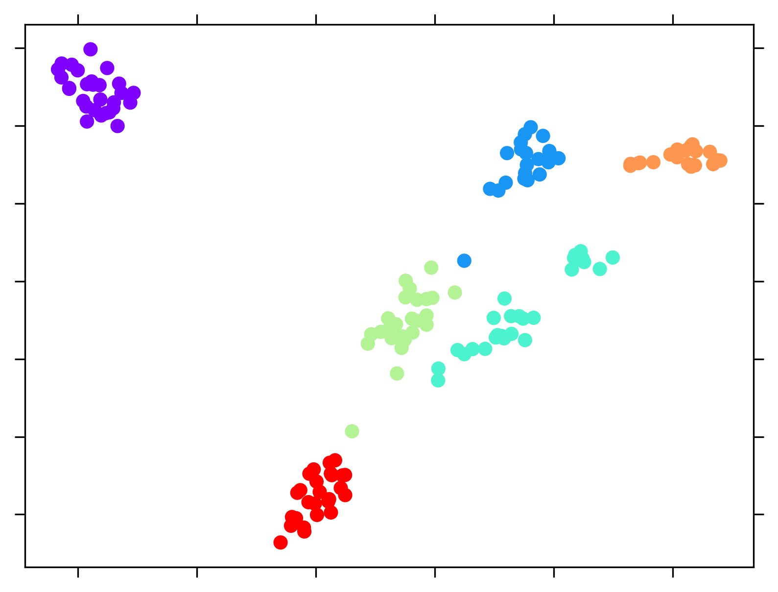
(b)

Tasks	F1 score
Train	0.7758 (0.056)
Test	0.6972 (0.107)

mean F1 score (standard error)

(c)

Figure 3: Causally heterogeneous synthetic datasets. We observe that our method performs better than the baselines, by pooling causally similar tasks identified using an embedding of causal mechanisms: (a) Generalisability performance reported as mean RMSE for the test tasks. (b) Example of the $\bm{z}$ embedding for the training tasks of one of the datasets, visualised in 2 dimensions using the t-SNE approach; colours indicate $C$ ground truth groups. (c) F1 scores of our method inferring the correct groups (for the training and unseen test tasks).

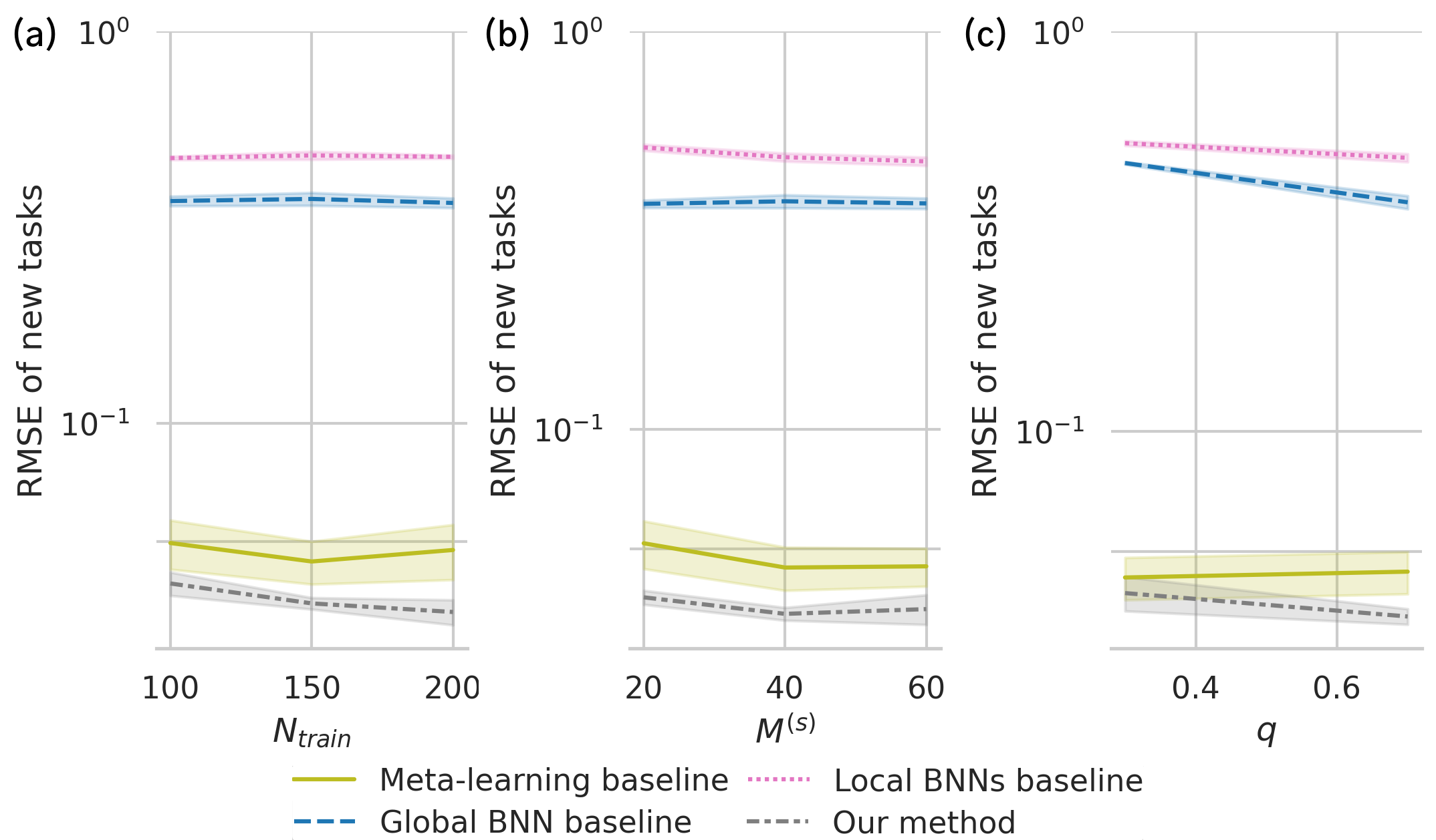
Figure 4: Sensitivity analyses. Generalisability performance (mean RMSE) for different synthetic data settings: (a) number of tasks; (b) number of samples per task; (c) ratio of interventional to observational data. We observe that our method performs consistently better than the baselines in limited data settings and leverages interventional data to identify relevant tasks for pooling.

Baselines and Ablations

The first group of baselines includes a global model “global BNN” (single neural network for all tasks), local BNNs that are trained on each task separately, and a Bayesian meta-learning baseline (Amit and Meir, 2018; Ravi and Beatson, 2018). We additionally consider two meta-learning methods that explicitly model task similarity: hierarchically structured meta-learning (HSML) (Yao et al., 2019a) and task similarity aware meta-learning (TSA-MAML) (Zhou et al., 2021), which model (non-causal) task similarity in terms of feature and model parameter similarity, respectively. In order to compare methods with similar model complexity, we use a comparable basic neural network architecture where possible, consisting of two linear layers, ReLU activation and 20 hidden units (except for the global model, where the number of parameters is doubled to exclude the possibility that hierarchical models trivially perform better because of a nested parameter structure).

We report the following ablations for our method: (i) without latent similarity - causally similar tasks are determined by comparing estimated $G_{t}$ instead of the latent space $\bm{z}_{t}$; (ii) without causal task similarity - similar tasks are determined in the parameter space of the BNN, instead of using the generative causal model; (iii) without task similarity - the task similarity aspect is removed entirely from the meta-learning method; (iv) without global hierarchy - the global parameters of the hierarchical model are removed (equivalent to training separate hierarchical models for each group of causally similar tasks). Further details for all baselines and ablations are given in Appendix B.2.

Performance Metrics

All methods are trained on $N_{\text{train}}$ tasks, validated on $N_{\text{val}}$ tasks, and evaluated on $N_{\text{test}}$ tasks to assess the methods’ generalisability performance. For the test tasks, $M^{(s)}$ support samples are used to derive task-specific models (for methods where this is applicable), then $M^{(q)}$ query samples are used to compute the evaluation metric $\ell$ (i.e., RMSE for regression or cross-entropy error for classification). For all experiments, this is averaged across $N_{\text{test}}$ tasks, $\frac{1}{N_{\text{test}}}\sum_{t=1}^{N_{\text{test}}}\ell(y_{t}^{(s)},y_{t,\text{pred}}^{(s)})$, and then averaged across 6 random dataset splits (or synthetic datasets). For synthetic data, we also report F1-scores for recovering the tasks’ ground truth causal groups.

Hyperparameters and Other Settings

Hyperparameters are selected based on the performance for the validation set and we report the results for the test set not used for hyperparameter tuning. A full list of hyperparameters and other settings used for each method is given in Appendix B.2.

6.2 Synthetic data results

We study datasets with causally heterogeneous task environments and report the results in Fig. 3, as well as a sensitivity analysis in Fig. 4. Unless stated otherwise in the text, synthetic datasets are generated using $N_{\text{train}}=150,N_{\text{val}}=N_{\text{test}}=30,M^{(s)}=M^{(q)}=40$, $C=6$, $q=0.7$. SCMs are generated with relatively low $\eta_{\text{task}}=0.001,\sigma_{\text{task}}=0.0001$ compared to $\eta_{\text{group}}=0.5,\sigma_{\text{group}}=0.02$, to form datasets with $C$ clusters of causally similar tasks (with small variation within clusters) related to a common reference SCM. We observe that our method has the following properties:

Improved generalisability in causally heterogeneous task environments

We observe that our method performs better than the global BNN, local BNNs and meta-learning baselines in the synthetic datasets with causally heterogeneous task environments. Results in Fig. 3a show that the generated datasets have the property that it is beneficial to pool data across tasks to improve task-level predictive performance (as indicated by global models performing better than local models, and meta-learning models performing better than global models), and that our method provides further benefit compared to the baseline meta-learning approach. A visualisation of the embedding in Fig. 3b and F1 scores in Fig. 3c show that the embedding can be used to identify groups of causally similar tasks, which are pooled by the predictive model to achieve better generalisability to new tasks from the same task environment.

Consistent performance in limited data settings

We observe that our method can aid generalisation performance in limited data settings. Fig. 3 shows that even for $N_{\text{train}}=150$ training tasks and $M^{(s)}=40$ support samples per task, causally similar tasks can be identified and utilised by the predictive model. A sensitivity analysis of a variety of settings for $N_{\text{train}}$ and $M^{(s)}$ is reported in Fig. 4a-b. In meta-learning, environment-level and task-level generalisation gaps result from having a finite number of tasks and samples per task (Rezazadeh, 2022; Amit and Meir, 2018; Pentina and Lampert, 2014). We observe this in our results, as well as that our method consistently has the lowest RMSE for various settings of $N_{\text{train}}$ and $M^{(s)}$.

Interventional data aids with identifying relevant tasks for pooling

Our method utilises interventional data to identify causally similar tasks for pooling. The sensitivity analysis of various settings of $q$ in Fig. 4c shows that our method has comparable performance with the meta-learning baseline for datasets with mostly observational data, and achieves lower RMSE for datasets with relatively more interventional data. This suggests that as intended, our method provides the most benefit for applications where data is observed under the effect of interventions (e.g., medical treatments, economic policy).

Table 1: Generalisability results in the three case studies (columns). We observe that our method provides improved generalisability performance, compared to meta-learning baselines (and a “no meta-learning” global model) including meta-learning methods that model task similarity using different approaches.

Method	Medical	Covid-19	Cognition
No meta.	0.854 (0.037)	0.729 (0.115)	1.727 (0.255)
Bayes. meta.	0.750 (0.049)	0.391 (0.110)	0.825 (0.173)
HSML	0.684 (0.074)	0.387 (0.086)	1.241 (0.142)
TSA-MAML	0.798 (0.071)	0.418 (0.116)	0.830 (0.037)
Our method	0.654 (0.036)	0.382 (0.106)	0.734 (0.208)

mean RMSE (standard error); best model for each dataset marked in bold

6.3 Health-related case studies

We compare meta-learning methods for 3 health-related use cases that represent illustrative examples of causally heterogeneous task environments, and which also contain interventional variables. As usual in real data, it cannot be guaranteed that these variables represent hard interventions (i.e., as assumed in (1)), and naturally we cannot study for certain whether our method actually learns from causally similar tasks in these cases. The results summarised in Table 1 show that our method performs better than the baselines for the datasets considered, including other meta-learning methods that utilise (non-causal) forms of task similarity. This indicates that the form of task similarity implemented in our method benefits generalisation performance.

Table 2: Ablation studies. Comparing our method with ablations (removing each of the listed components in turn), we observe that a latent generative model of causal mechanisms and hierarchical modelling contribute to improved generalisability performance; we see similar results when accounting for settings of less data per task and less interventional data. See text for further details.

	Synthetic dataset
	RMSE	F1 score
Method	New tasks	Train tasks	New tasks
Our method	0.0376 (0.002)	0.7493 (0.053)	0.6403 (0.110)
- Latent similarity	0.0520 (0.006)	0.1545 (0.012)	0.0516 (0.019)
- Causal task similarity	0.0517 (0.006)	0.2177 (0.008)	0.0634 (0.018)
- Task similarity	0.0453 (0.005)	NA	NA
- Global pooling	0.0533 (0.003)	NA	NA
	Less data per task ($M^{(s)}$)
	RMSE	F1 score
Method	New tasks	Train tasks	New tasks
Our method	0.0403 (0.001)	0.7415 (0.044)	0.6007 (0.057)
- Latent similarity	0.0563 (0.008)	0.1598 (0.005)	0.0554 (0.013)
- Causal task similarity	0.0589 (0.008)	0.2264 (0.004)	0.0626 (0.014)
- Task similarity	0.0522 (0.007)	NA	NA
- Global pooling	0.0544 (0.004)	NA	NA
	Less interventional data ($q$)
	RMSE	F1 score
Method	New tasks	Train tasks	New tasks
Our method	0.0373 (0.003)	0.6845 (0.072)	0.6575 (0.072)
- Latent similarity	0.0467 (0.006)	0.1560 (0.008)	0.0824 (0.016)
- Causal task similarity	0.0492 (0.006)	0.2181 (0.003)	0.0536 (0.016)
- Task similarity	0.0408 (0.004)	NA	NA
- Global pooling	0.0541 (0.003)	NA	NA

mean RMSE (standard error) and mean F1 scores (standard error); best models marked in bold; F1 score is NA if method does not use task similarity or uses same groups as full method

6.4 Ablation studies

To better understand what aspects of our method contribute to improved generalisability performance we setup controlled ablation studies for synthetic datasets, reported in Table 2. We consider three datasets of interest motivated by practical concerns: (i) a causally heterogeneous task environment, $C=6,\eta_{\text{group}}=0.5$ (reference setup); (ii) the reference setup with less data per task ($M^{(s)}=20$ instead of $M^{(s)}=40$); (iii) the reference setup with relatively less interventional data ($q=0.5$ instead of $q=0.7$). All other hyperparameters are the same as Sec. 6.2.

The results in Table 2 show that several aspects of the method contribute to its performance. In particular, the use of the latent space $\bm{z}_{t}$, as opposed to directly measuring causal distances between inferred DAGs $\mathcal{G}_{t}$, aids identifiability of causally similar tasks (indicated by the drop in F1 scores for the without latent similarity ablation). This result emphasises that it is challenging to completely identify the task SCMs from the data, but the embedding is a useful approach for identifying groups of tasks with similar SCMs, which in this case is sufficient for improving predictive performance. The poorer performance for the without causal task similarity ablation also shows that the causal generative model used in experiments is more effective than an alternative approach of calculating task similarity in the predictive model parameter space (which we observe generalises more poorly to unseen tasks, compared to our approach). The hierarchical model also contributes to improved generalisability performance, as indicated by weaker performance in the without task similarity (removing the group parameters $\bm{\theta}_{c}$) and without global hierarchy (removing the global parameters $\bm{\theta}$) ablations, illustrating the benefits of pooling data at multiple levels.

7 Discussion and conclusion

In this paper we proposed a new problem setting and method for meta-learning predictive models in causally heterogeneous task environments, where tasks may be generated by different causal mechanisms. In a range of experiments on simulated and real datasets, we showed that our method improves generalisability performance for causally heterogeneous datasets, without knowledge of the true causal models for tasks. Ablation studies showed that a latent generative model of causal mechanisms (represented by structural causal models) and hierarchical modelling (in the predictive model) contribute to the improved performance.

However, there are some limitations and open problems. The paper is best seen as a proof of concept, after which many details can be improved in future work and for specific use cases. Here we used an embedding of causal models learned separately, and a natural question is how much performance could be improved by either adding considerably more data to such a “foundation model”, or different kinds of data such as simulated data from counterfactual scenarios. Another natural question is how much would estimating the two models together help, which is expected to be relevant in scenarios with less total data. Finally, if computation can be made feasible for the new initiative of hierarchical causal models (Weinstein and Blei, 2024), identifiability of the mechanisms has potential to improve considerably.

8 Acknowledgements

This study has received funding from the European Union’s Horizon 2020 research and innovation programme under grant agreement No 101016775. This research has been conducted using the UK Biobank Resource under Application Number 77565.

Appendix A Further details for our method

A.1 Algorithms

Algorithm 1 Meta-learning

  Require: Tasks $\mathcal{D}_{1},...,\mathcal{D}_{N}$; learning rates $\beta_{1},\beta_{2}$; number of updates $G$

  Initialise: $\bm{\psi}^{(0)}$, $\bm{\psi}_{c}^{(0)}$ for $c=1,...,C$, prior distributions for parameters, and $\bm{z}_{1},...,\bm{z}_{N}$ as per the procedure described in Sec. 5

  Construct $\tilde{D}\in\mathbb{R}^{N\times N}$ from $d(t_{i},t_{j})$ for $i,j=1,...,N$ and apply spectral clustering to determine the causal group assignments $c_{1},...,c_{N}$

  for $t=0$ to $N-1$ do

     Sample $\mathcal{D}_{t}^{(s)},\mathcal{D}_{t}^{(q)}$ from $\mathcal{D}_{t}$

     Initialise $\bm{\gamma}_{t}^{(0)}$ and $p(\bm{\phi}_{t}\mid\bm{\theta}_{c},\bm{\theta})=N(\bm{\phi}_{t};\bm{\mu}_{\bm{\psi}_{c_{t}}}^{(t)},{\bm{\sigma}^{2}}^{(t)}_{\bm{\psi}_{c_{t}}}\bm{I})$

     for $g=0$ to $G-1$ do

        $\bm{\gamma}_{t}^{(g+1)}\leftarrow\bm{\gamma}_{t}^{(g)}-\beta_{1}\nabla_{\bm{\gamma}_{t}}\mathcal{L}_{\mathcal{D}_{t}^{(s)}}(\bm{\gamma}_{t}^{(g)})$

     end for

     $\bm{\psi}_{c_{t}}^{(t+1)}\leftarrow\bm{\psi}_{c_{t}}^{(t)}-\beta_{2}\nabla_{\bm{\psi}_{c_{t}}}\big{[}\mathcal{L}_{{\mathcal{D}}_{t}}(\bm{\gamma}_{t}^{(G-1)})+\frac{1}{N_{c}}D_{KL}(q_{\bm{\psi}_{c_{t}}}(\bm{\theta}_{c_{t}})\;\|\;p(\bm{\theta}_{c_{t}}\mid\bm{\theta}))\big{]}$

     $\bm{\psi}^{(t+1)}\leftarrow\bm{\psi}^{(t)}-\beta_{2}\nabla_{\bm{\psi}}\big{[}\mathcal{L}_{{\mathcal{D}}_{t}}(\bm{\gamma}_{t}^{(G-1)})+\frac{1}{N_{c}}D_{KL}(q_{\bm{\psi}_{c_{t}}}(\bm{\theta}_{c_{t}})\;\|\;p(\bm{\theta}_{c_{t}}\mid\bm{\theta}))+\frac{1}{N}D_{KL}(q_{\bm{\psi}}(\bm{\theta})\;\|\;p(\bm{\theta}))\big{]}$

     $p(\bm{\theta}_{c}\mid\bm{\theta})=N(\bm{\theta}_{c};\bm{\mu}_{\bm{\psi}}^{(t+1)},{\bm{\sigma}^{2}}^{(t+1)}_{\bm{\psi}}\bm{I})$ for $c=1,...,C$

  end for

Algorithm 2 Adapting to new tasks

  Require: New task $\mathcal{D}_{t}$; learning rate $\beta_{1}$; number of updates $G$; number of samples $S$; representative embeddings $\bm{z}^{1},...,\bm{z}^{C}$

  Initialise: $\bm{z}_{t}$ and the group $c_{t}$ that minimises $d(\bm{z}_{t},\bm{z}^{c_{t}})$; $\bm{\gamma}_{t}^{(0)}=\{\bm{\mu}_{\bm{\psi}_{c_{t}}},{\bm{\sigma}^{2}}_{\bm{\psi}_{c_{t}}}\}$, and $p(\bm{\phi}_{t}\mid\bm{\theta}_{c},\bm{\theta})=N(\bm{\phi}_{t};\bm{\mu}_{\bm{\psi}_{c_{t}}},{\bm{\sigma}^{2}}_{\bm{\psi}_{c_{t}}}\bm{I})$ from Alg 1

  for $g=0$ to $G-1$ do

     $\bm{\gamma}_{t}^{(g+1)}\leftarrow\bm{\gamma}_{t}^{(g)}-\beta_{1}\nabla_{\bm{\gamma}_{t}}\mathcal{L}_{\mathcal{D}_{t}^{(s)}}(\bm{\gamma}_{t}^{(g)})$

  end for

  for $s=0$ to $S-1$ do

     Sample $\bm{\phi}_{t}^{s}\sim N(\bm{\phi}_{t};\bm{\mu}^{(G-1)}_{\bm{\gamma}_{t}},{\bm{\sigma}^{2}}^{(G-1)}_{\bm{\gamma}_{t}}\bm{I})$

  end for

  Evaluate $p(\bm{y}_{t}^{(q)}\mid\bm{x}_{t}^{(q)},\mathcal{D}_{t}^{(s)},\bm{\theta}_{c_{t}})\approx\frac{1}{S}\sum_{s=1}^{S}p(\bm{y}_{t}^{(q)}\mid\bm{x}_{t}^{(q)},\bm{\phi}_{t}^{s})$

A.2 Optimisation objective

The posterior distribution over the neural network parameters is

$$p(\bm{\theta},\bm{\theta}_{1},...,\bm{\theta}_{C},\bm{\phi}_{1},...,\bm{\phi}_{N}\mid\mathcal{D}_{1},...,\mathcal{D}_{N})=p(\bm{\theta}\mid\mathcal{D}_{1},...,\mathcal{D}_{N})\prod_{c=1}^{C}p(\bm{\theta}_{c}\mid\bm{\theta},\mathcal{D}_{1},...,\mathcal{D}_{N_{c}})\prod_{i=1}^{N}p(\bm{\phi_{i}}\mid\bm{\theta}_{c_{i}},\mathcal{D}_{i}),$$ (11)

which is approximated using a family of variational distributions:

$$q(\bm{\theta},\bm{\theta}_{1},...,\bm{\theta}_{C},\bm{\phi}_{1},...,\bm{\phi}_{N})=q_{\bm{\psi}}(\bm{\theta})\prod_{c=1}^{C}q_{\bm{\psi}_{c}}(\bm{\theta}_{c})\prod_{i=1}^{N}q_{\bm{\gamma}_{i}}(\bm{\phi}_{i}),$$ (12)

where $\bm{\psi},\bm{\psi}_{1},...,\bm{\psi}_{C},\bm{\gamma}_{1},...,\bm{\gamma}_{N}$ are unknown (variational) parameters.

The following optimisation problem is solved to obtain an approximation for the variational parameters:

$$\underset{\bm{\psi},\bm{\psi}_{1},...,\bm{\psi}_{C},\bm{\gamma}_{1},...,\bm{\gamma}_{N}}{\operatorname{argmin}}D_{KL}(q(\bm{\theta},\bm{\theta}_{1},\ldots,\bm{\theta}_{C},\bm{\phi}_{1},\ldots,\bm{\phi}_{N})\;\|\;p(\bm{\theta},\bm{\theta}_{1},\ldots,\bm{\theta}_{C},\bm{\phi}_{1},\ldots,\bm{\phi}_{N}|\mathcal{D}_{1},\ldots,\mathcal{D}_{N}))\\ =\underset{\bm{\psi},\bm{\psi}_{1},...,\bm{\psi}_{C},\bm{\gamma}_{1},...,\bm{\gamma}_{N}}{\operatorname{argmin}}D_{KL}(q_{\bm{\psi}}(\bm{\theta})\prod_{c=1}^{C}q_{\bm{\psi}_{c}}(\bm{\theta}_{c})\prod_{i=1}^{N}q_{\bm{\gamma}_{i}}(\bm{\phi}_{i})\;\|\;p(\bm{\theta}\mid\mathcal{D}_{1},...,\mathcal{D}_{N})\prod_{c=1}^{C}p(\bm{\theta}_{c}\mid\bm{\theta},\mathcal{D}_{1},...,\mathcal{D}_{N_{c}})\prod_{i=1}^{N}p(\bm{\phi_{i}}\mid\bm{\theta}_{c_{i}},\mathcal{D}_{i})),$$ (13)

where $D_{KL}(\cdot\;\|\;\cdot)$ is the Kullback-Leibler divergence, defined as

$$D_{KL}(q\;\|\;p)\triangleq\int q(x)\log\frac{q(x)}{p(x)}\,dx.$$ (14)

Using (14), an equivalent form for the optimisation problem (13) is derived:

$$\underset{\bm{\psi},\bm{\psi}_{1},...,\bm{\psi}_{C},\bm{\gamma}_{1},...,\bm{\gamma}_{N}}{\operatorname{argmin}}\mathbb{E}_{q_{\bm{\psi}}}\big{[}\mathbb{E}_{q_{\bm{\psi_{c}}}}\big{[}\mathbb{E}_{q_{\bm{\gamma}_{i}}}\big{[}\log q_{\bm{\psi}}(\bm{\theta})+\sum_{c=1}^{C}\log q_{\bm{\psi_{c}}}(\bm{\theta}_{c})+\sum_{i=1}^{N}\log q_{\bm{\gamma_{i}}}(\bm{\phi_{i}})\\ -\log p(\bm{\theta}|\mathcal{D}_{1},\ldots,\mathcal{D}_{N})-\sum_{c=1}^{C}\log p(\bm{\theta}_{c}|\mathcal{D}_{1},\ldots,\mathcal{D}_{N_{c}})-\sum_{i=1}^{N}\log p(\bm{\phi_{i}}|\bm{\theta}_{c_{i}},\mathcal{D}_{i})\big{]}\big{]}\big{]}.$$ (15)

The following are derived using Bayes’ theorem and conditional independence in the model (Fig. 2c):

$$p(\bm{\theta}|\mathcal{D}_{1},\ldots,\mathcal{D}_{N})=\frac{\prod_{i=1}^{N}p(\mathcal{D}_{i}|\bm{\theta})p(\bm{\theta})}{p(\mathcal{D}_{1},\ldots,\mathcal{D}_{N})},$$ (16)

$$p(\bm{\theta}_{c}|\bm{\theta},\mathcal{D}_{1},\ldots,\mathcal{D}_{N})=\frac{\prod_{i=1}^{N_{c}}p(\mathcal{D}_{i}|\bm{\theta},\bm{\theta}_{c})p(\bm{\theta}_{c}|\bm{\theta})}{\prod_{i=1}^{N_{c}}p(\mathcal{D}_{i}|\bm{\theta})}=\frac{\prod_{i=1}^{N_{c}}p(\mathcal{D}_{i}|\bm{\theta}_{c})p(\bm{\theta}_{c}|\bm{\theta})}{\prod_{i=1}^{N_{c}}p(\mathcal{D}_{i}|\bm{\theta})},$$ (17)

$$p(\bm{\phi}_{i}|\bm{\theta}_{c},\mathcal{D}_{i})=\frac{p(\mathcal{D}_{i}|\bm{\phi}_{i},\bm{\theta}_{c})p(\bm{\phi}_{i}|\bm{\theta}_{c})}{p(\mathcal{D}_{i}|\bm{\theta}_{c})}=\frac{p(\mathcal{D}_{i}|\bm{\phi}_{i})p(\bm{\phi}_{i}|\bm{\theta}_{c})}{p(\mathcal{D}_{i}|\bm{\theta}_{c})}.$$ (18)

Substituting (16), (17) and (18) into (15), and dropping terms that are independent of the optimisation parameters and rearranging gives

$$\underset{\bm{\psi},\bm{\psi}_{1},...,\bm{\psi}_{C},\bm{\gamma}_{1},...,\bm{\gamma}_{N}}{\operatorname{argmin}}\mathbb{E}_{q_{\bm{\psi}}}\big{[}\mathbb{E}_{q_{\bm{\psi_{c}}}}\big{[}\mathbb{E}_{q_{\bm{\gamma}_{i}}}\big{[}{\color[rgb]{1,.5,0}\log q_{\bm{\psi}}(\bm{\theta})}+{\color[rgb]{0,0,1}\sum_{c=1}^{C}\log q_{\bm{\psi_{c}}}(\bm{\theta}_{c})}+{\color[rgb]{0,.5,.5}\sum_{i=1}^{N}\log q_{\bm{\gamma_{i}}}(\bm{\phi_{i}})}-\sum_{i=1}^{N}\log p(\mathcal{D}_{i}|\bm{\theta})-{\color[rgb]{1,.5,0}\log p(\bm{\theta})}\\ +\log p(\mathcal{D}_{1},\ldots,\mathcal{D}_{N})-\sum_{c=1}^{C}\sum_{i=1}^{N_{c}}\log p(\mathcal{D}_{i}|\bm{\theta}_{c})-{\color[rgb]{0,0,1}\sum_{c=1}^{C}\log p(\bm{\theta}_{c}|\bm{\theta})}+\sum_{c=1}^{C}\sum_{i=1}^{N_{c}}\log p(\mathcal{D}_{i}|\bm{\theta})-\sum_{i=1}^{N}{\color[rgb]{1,0,1}\log p(\mathcal{D}_{i}|\bm{\phi}_{i})}\\ -{\color[rgb]{0,.5,.5}\sum_{i=1}^{N}\log p(\bm{\phi}_{i}|\bm{\theta}_{c_{i}})}+\sum_{i=1}^{N}\log p(\mathcal{D}_{i}|\bm{\theta}_{c_{i}})\big{]}\big{]}\big{]}\\ =\underset{\bm{\psi},\bm{\psi}_{1},...,\bm{\psi}_{C},\bm{\gamma}_{1},...,\bm{\gamma}_{N}}{\operatorname{argmin}}\mathbb{E}_{q_{\bm{\psi}}}\big{[}{\color[rgb]{1,.5,0}\log\frac{q_{\bm{\psi}}(\bm{\theta})}{p(\bm{\theta})}}\big{]}+\mathbb{E}_{q_{\bm{\psi}}}\big{[}\sum_{c=1}^{C}\mathbb{E}_{q_{\bm{\psi_{c}}}}\big{[}{\color[rgb]{0,0,1}\log\frac{q_{\bm{\psi_{c}}}(\bm{\theta}_{c})}{p(\bm{\theta}_{c}|\bm{\theta})}}\big{]}\big{]}+\mathbb{E}_{q_{\bm{\psi}}}\big{[}\sum_{c=1}^{C}\mathbb{E}_{q_{\bm{\psi_{c}}}}\big{[}\sum_{i=1}^{N_{c}}\mathbb{E}_{q_{\bm{\gamma}_{i}}}\big{[}{\color[rgb]{0,.5,.5}\log\frac{q_{\bm{\gamma_{i}}}(\bm{\phi_{i}})}{p(\bm{\phi}_{i}|\bm{\theta}_{c})}}\\ -{\color[rgb]{1,0,1}\log p(\mathcal{D}_{i}|\bm{\phi}_{i})}-\log p(\mathcal{D}_{i}|\bm{\theta})+\log p(\mathcal{D}_{i}|\bm{\theta})+\log p(\mathcal{D}_{i}|\bm{\theta}_{c})-\log p(\mathcal{D}_{i}|\bm{\theta}_{c})\big{]}\big{]}\big{]}\\ =\underset{\bm{\psi},\bm{\psi}_{1},...,\bm{\psi}_{C},\bm{\gamma}_{1},...,\bm{\gamma}_{N}}{\operatorname{argmin}}{\color[rgb]{1,.5,0}D_{KL}(q_{\bm{\psi}}(\bm{\theta})\;\|\;p(\bm{\theta}))}+{\color[rgb]{0,0,1}D_{KL}(q_{\bm{\psi_{c}}}(\bm{\theta}_{c})\;\|\;p(\bm{\theta}_{c}|\bm{\theta}))}+{\color[rgb]{0,.5,.5}D_{KL}(q_{\bm{\gamma_{i}}}(\bm{\phi_{i}})\;\|\;p(\bm{\phi}_{i}|\bm{\theta}_{c}))}-\\ \mathbb{E}_{q_{\bm{\psi}}}\big{[}\sum_{c=1}^{C}\mathbb{E}_{q_{\bm{\psi_{c}}}}\big{[}\sum_{i=1}^{N_{c}}\mathbb{E}_{q_{\bm{\gamma}_{i}}}\big{[}{\color[rgb]{1,0,1}\log p(\mathcal{D}_{i}|\bm{\phi}_{i})}\big{]}\big{]}\big{]}.$$

This optimisation objective can be rewritten as

$$\underset{\bm{\psi},\bm{\psi}_{1},...,\bm{\psi}_{C},\bm{\gamma}_{1},...,\bm{\gamma}_{N}}{\operatorname{argmin}}\mathbb{E}_{q_{\bm{\psi}}}\big{[}\sum_{c=1}^{C}\mathbb{E}_{q_{\bm{\psi}_{c}}}\big{[}\sum_{i=1}^{N_{c}}\mathcal{L}_{\mathcal{D}_{i}}(\bm{\gamma}_{i})\big{]}+D_{KL}(q_{\bm{\psi}_{c}}(\bm{\theta}_{c})\;\|\;p(\bm{\theta}_{c}\mid\bm{\theta}))\big{]}+D_{KL}(q_{\bm{\psi}}(\bm{\theta})\;\|\;p(\bm{\theta})),$$ (19)

where the part of the optimisation objective corresponding to the task data is denoted by

$$\mathcal{L}_{\mathcal{D}_{i}}(\bm{\gamma}_{i})=D_{KL}(q_{\bm{\gamma}_{i}}(\bm{\phi}_{i}\mid\mathcal{D}_{i})\;\|\;p(\bm{\phi}_{i}\mid\bm{\theta_{c}}))-\mathbb{E}_{q_{\bm{\gamma}_{i}}}[\log p(\mathcal{D}_{i}\mid\bm{\phi}_{i})].$$ (20)

It is convention in meta-learning to split the data for each training task into support and query samples to improve generalisation: $\mathcal{D}_{i}=\mathcal{D}_{i}^{(s)}\cup\mathcal{D}_{i}^{(q)}$. In this case, we use $\mathcal{L}_{\mathcal{D}_{i}^{(s)}}(\bm{\gamma}_{i})$ when updating the local parameters, while the query set is used to evaluate the local model’s performance and update the group and global parameters. Algorithms 1 and 2 give details for how the optimisation procedure is implemented in experiments for Bayesian neural networks (BNNs).

A.3 Additional implementation details

Architecture

For the BNN architecture we used two Bayesian linear layers, each followed by a rectified linear unit (ReLU) activation function. Each of these layers comprises 20 hidden units.

Priors and initialisation

The BNN priors are given in (10). We observed significant improvement by initialising the (global) BNN parameters based on a few training iterations of a basic hierarchical model (Fig. 2b).

Training and early stopping

We use an early stopping criterion that stops the model training when validation loss increases. This prevents overfitting and reduces the computational cost of training. BNNs often suffer from the cold posterior effect. To alleviate this, we incorporated a weight $\lambda$ in the optimisation objective.

Additional details for the causal generative model

For the generative model, the prior is given in (5), and in experiments we consider Erdős-Rényi graph priors $p(\mathcal{G})\propto q^{{\lVert\mathcal{G}\rVert}_{1}}(1-q)^{\binom{K+1}{2}-{\lVert\mathcal{G}\rVert}_{1}}$ (which encodes prior knowledge that each edge exists independently with probability $q$) and scale-free graph priors $p(\mathcal{G})\propto\prod_{k=1}^{K+1}(1+{\lVert\mathcal{G}_{k}^{T}\rVert}_{1})^{-3}$. These priors are each added as an additional term in (5). In experiments we use linear Gaussian SCM and non-linear Gaussian SCM models (2-layers with 5 hidden nodes):

$$p(\tilde{\bm{x}}_{t}\mid\mathcal{G}_{t},\bm{\Theta}_{t})=N(\tilde{\bm{x}}_{t};(\mathcal{G}_{t}\odot\bm{\Theta}_{t})^{T}\tilde{\bm{x}}_{t},\sigma^{2}\bm{I}),$$

for a linear Gaussian SCM and

$$p(\tilde{\bm{x}}_{t}\mid\mathcal{G}_{t},\bm{\Theta}_{t})=\prod_{k=1}^{K+1}N(\tilde{\bm{x}}_{t,k};\text{FFN}(\mathcal{G}_{t,k}^{T}\odot\tilde{\bm{x}}_{t};\bm{\Theta}_{t,k}),\sigma^{2}),$$

for a non-linear Gaussian SCM, where FFN is a feed-forward neural network, $\odot$ denotes element-wise multiplication, and $\tilde{\bm{x}}_{t}$ refers to a data input consisting of both $\bm{x}_{t}$ and $\bm{y}_{t}$.

As described in the main text, we use the Stein variational gradient descent routine implemented by Lorch et al. [2021] for generating the side data $\bm{z}_{t}$ for our predictive model. The model is first trained using the data for all $N$ tasks and then fine-tuned to each task to infer $p(\bm{z}_{t}\mid\mathcal{D}_{t})$.

Appendix B Further details for experiments

B.1 Datasets

Table 3 summarises the datasets used in experiments, where $N_{\text{train}}$ is number of training tasks, $N_{\text{val}}$ is number of validation tasks, $N_{\text{test}}$ is number of test tasks, $M^{(s)}$ is number of support samples per task, $M^{(q)}$ is number of query samples per task. For all experiments, the models are trained and evaluated for 5 random dataset splits.

Table 3: Overview of datasets used in experiments. Synthetic data experiments use the data splits specified here, unless explicitly stated otherwise in the text.

	$N_{\text{train}}$	$N_{\text{val}}$	$N_{\text{test}}$	$M^{(s)}$	$M^{(q)}$
Synthetic	200	30	30	30	30
Medical	217	46	46	6	6
COVID-19	114	24	24	15	14
Cognition	16	3	3	120	120

Synthetic dataset

Synthetic data is simulated from linear Gaussian SCMs defined for each task:

$$V_{u}:=\sum_{v\in\operatorname{\textbf{PA}}_{u}^{\mathcal{G}}}\beta_{v}V_{v}+\epsilon_{u}.$$

The hyperparameters of the synthetic data model include the number of train, validation and test tasks $N_{\text{train}},N_{\text{val}},N_{\text{test}}$, number of support and query samples per task $M^{(s)},M^{(q)}$, random seed, variance for reference SCM parameters $\sigma_{\text{ref}}$, Gaussian noise variance $\sigma_{\text{noise}}$, and the ratio of observational to interventional data $q$. The properties of the task environment are determined by hyperparameters that control how similar or different the causal models are between groups of causally similar tasks and individual tasks. Specifically, $C$ is the number of groups of causally similar tasks, $\eta_{\text{group}}$ controls variation of DAGs across groups, $\eta_{\text{task}}$ controls variation of DAGs within groups, $\sigma_{\text{group}}$ controls variation of group SCM parameters (relative to the reference parameters), and $\sigma_{\text{task}}$ controls variation of task SCM parameters (relative to the group parameters).

In experiments, a reference model for each dataset $(\mathcal{G}_{\text{ref}},\bm{\beta}_{\text{ref}})$ is randomly generated for $K+1=8$ nodes with expected degree 2, where $\beta_{k}^{\text{ref}}\sim N(0,\sigma_{\text{ref}})$ for $k=0,...,K+1$. The $Y$ node is chosen as the node with the highest number of parents and no children. SCMs for $C$ groups of causally similar tasks are derived from $(\mathcal{G}_{\text{ref}},\bm{\beta}_{\text{ref}})$ using two hyperparameters $(\sigma_{\text{group}},\eta_{\text{group}})$, where $\bm{\beta}_{c}\sim N(\bm{\beta}_{\text{ref}},\sigma_{\text{group}})$ and $\mathcal{G}_{c}$ is determined by “flipping” edges in the adjacency matrix of $\mathcal{G}_{\text{ref}}$ with probability $p\sim\text{Unif}(0,\eta_{\text{group}})$. Tasks are assigned to $C$ causal groups and a task model is derived in a similar hierarchical manner, where variation from the corresponding group model is determined by $(\sigma_{\text{task}},\eta_{\text{task}})$.

$M=M^{(s)}+M^{(q)}$ data samples are generated for each of the $N$ tasks from the corresponding task SCMs, for the train, validation and test sets. For each data sample, a (predetermined) hard intervention occurs with probability $q$ (otherwise the data sample is considered observational). The $Y$ values are rescaled between 0 and 1 by applying the sigmoid function to create a label for the prediction task (which can be easily modified for regression or binary classification tasks).

Medical dataset

The variables listed in Table 4 are extracted from the UK Biobank dataset bycroft2018uk for 309 patients (tasks) with a diagnosis of type 2 diabetes (T2D) prior to January 1, 2000. After the variables are extracted and quality checked for outliers and other issues, year-level data is derived between 2000 and 2020. The intervention variables are defined as binary variables with value 1 if the treatment was prescribed in a given year and 0 otherwise. The diagnosis variables are defined as binary variables with value 1 if the patient received the diagnosis prior to the given year and 0 otherwise. The other variables and the label are continuous variables defined as the average value for the given year or the most recent value from the previous year. The datasets are then prepared according to the data splits described in Table 3.

The final dataset consists of 309 patients with 12 datapoints each. The cohort is 64.7% female, with a mean age of 59 years and mean age of 49 at T2D diagnosis. The most frequent treatment is Simvastatin (38% of observations), followed by Atorvastatin (28% of observations), and other statins (7.7% of observations). The most common diagnosis is CAD (35%), followed by Stroke (3.0%), AAA (0.3%) and DVT (0.1%). The mean total cholesterol level is 4.39 mmol/L. For other variables, the mean values are as follows: 31.5 for BMI, 77.5 mmHG for DBP, 135.6 mmHg for SBP.

We obtained permission to use the UK Biobank resource under application number 77565.

Table 4: Variables used in the medical dataset. The data source is the UK Biobank dataset bycroft2018uk. Full details of the UK Biobank data fields are available at https://biobank.ndph.ox.ac.uk/showcase/

Variable name (type)	Data source
Total cholesterol (label)	Values are derived from the participant’s GP clinical event records (field 42040) for read v2 codes that matched 44P.. and read v3 codes that matched XE2eD
Atorvastatin (intervention)	Prescription dates are derived from the participant’s GP prescription records (field 42039) for drug names that matched “atorvastatin”, “lipitor”
Simvastatin (intervention)	Prescription dates are derived from the participant’s GP prescription records (field 42039) for drug names that matched “simvastatin”, “zocor”
Other statin (intervention)	Prescription dates are derived from the participant’s GP prescription records (field 42039) for drug names that matched “pravastatin”, “pravachol”, ‘rosuvastatin”, “crestor”, “ezallor’
Coronary Artery Disease (diagnosis)	Date of first report derived from fields 131306 (I25), 131304 (I24), 131302 (I23), 131300 (I22), 131298 (I21), 131296 (I20)
Stroke (diagnosis)	Date of first report derived from fields 131378 (I69), 131374 (I67), 131372 (I66), 131366 (I63), 131058 (G46)
Abdominal Aortic Aneurysm (diagnosis)	Date of first report derived from fields 131394 (I79), 131382 (I71)
Deep Vein Thrombosis (diagnosis)	Date of first report derived from fields 132198 (O22), 131400 (I82)
Systolic blood pressure (other)	Values are derived from the participant’s GP clinical event records (field 42040) for read v2 codes that matched 2469. and read v3 codes that matched 2469.
Diastolic blood pressure (other)	Values are derived from the participant’s GP clinical event records (field 42040) for read v2 codes that matched 246A and read v3 codes that matched 246A
Body mass index (other)	Values are derived from the participant’s GP clinical event records (field 42040) for read v2 codes that matched 22K.. and read v3 codes that matched 22K..
Sex (other)	Genetic sex of the participant (field 31)
Age (other)	Age derived from the year of birth of the participant (field 34)

COVID-19 dataset

The variables listed in Table 5 are extracted from the Response2covid19 dataset porcher2020response2covid19 for 162 countries (tasks). After the variables are extracted, week-level data is derived for 2020. The values for the intervention variables are averaged for the given week (i.e., maximum value of 1 for all days in the week, minimum value of 0 for no days that week). The other variables are defined as described in Table 5. The datasets are then prepared according to the data splits described in Table 3.

Table 5: Variables used in the COIVD-19 dataset. The data source is the Response2covid19 dataset porcher2020response2covid19

Variable name (type)	Data source
Covid cases (label)	Response2covid19 dataset, total number of cases reported each week
School (intervention)	Response2covid19 dataset, indicating if schools were closed
Domestic (intervention)	Response2covid19 dataset, indicating if there was a domestic lockdown
Travel (intervention)	Response2covid19 dataset, indicating if travel restrictions were implemented
Travel dom (intervention)	Response2covid19 dataset, indicating if there were travel restrictions within the country (e.g. inter-region travels)
Curf (intervention)	Response2covid19 dataset, indicating if a curfew was implemented
Mass (intervention)	Response2covid19 dataset, indicating if bans on mass gatherings were implemented
Sport (intervention)	Response2covid19 dataset, indicating if bans on sporting and large events were implemented
Rest (intervention)	Response2covid19 dataset, indicating if restaurants were closed
Testing (intervention)	Response2covid19 dataset, indicating if there was a public testing policy
Masks (intervention)	Response2covid19 dataset, indicating if mandates to wear masks in public spaces were implemented
Surveillance (intervention)	Response2covid19 dataset, indicating if mobile app or bracelet surveillance was implemented
State (intervention)	Response2covid19 dataset, indicating if the state of emergency is declared
Population (other)	Other, population size for the country in 2020
Week (other)	NA, week number since start of 2020

Cognition dataset

The variables listed in Table 6 are extracted from the CogLoad dataset gjoreski2020datasets for 22 individuals (tasks). There are 240 observations extracted for each individual, including variables for physiological responses, personality traits and cognitive load when performing computer-based tasks of varying levels of difficulty. Aside from separating the difficulty level into 3 separate indicator variables, we do not perform any other transformations to the data. The datasets are then prepared according to the data splits described in Table 3.

Table 6: Variables used in the cognition dataset. The data source is the CogLoad dataset gjoreski2020datasets

Variable name (type)	Data source
Points (label)	CogLoad dataset, number of points scored in the task
Level 0 (intervention)	CogLoad dataset, binary indicator for task difficulty level 0
Level 1 (intervention)	CogLoad dataset, binary indicator for task difficulty level 1
Level 2 (intervention)	CogLoad dataset, binary indicator for task difficulty level 2
hr (other)	CogLoad dataset, heart rate
gsr (other)	CogLoad dataset, galvanic skin response
rr (other)	CogLoad dataset, RR intervals
temperature (other)	CogLoad dataset, skin temperature
click per second (other)	CogLoad dataset, number of clicks the participant made during the measuring time
honesty (other)	CogLoad dataset, personality trait
emotionality (other)	CogLoad dataset, personality trait
extraversion (other)	CogLoad dataset, personality trait
agreeableness (other)	CogLoad dataset, personality trait
conscientiousness (other)	CogLoad dataset, personality trait
openness (other)	CogLoad dataset, personality trait

B.2 Baselines, ablations and hyperparameter settings

For all methods, hyperparameters are selected based on performance for the validation tasks and the final result is reported for the test tasks.

Global BNN baseline

The BNN consists of two Bayesian linear layers with ReLU activation and 20 hidden units. The method is implemented using stochastic variational inference (SVI) from the NumPyro library phan2019composable, bingham2019pyro. The model is trained by combining the feature and label data for all training tasks (for both support and query samples) into one feature matrix and one label vector. The model is validated and evaluated using the query samples for the validation and test tasks. Other hyperparameter settings considered: learning rate 0.001, 0.0001.

Individual BNNs baseline

Similar to the global baseline, each BNN consists of two Bayesian linear layers with ReLU activation and 20 hidden units, implemented using SVI from the NumPyro library phan2019composable, bingham2019pyro. For each task, a model is trained using the support samples and evaluation metrics are computed using the query samples. Other hyperparameter settings considered: learning rate 0.001, 0.0001.

Bayesian meta-learning baseline

The Bayesian meta-learning algorithm is implemented using the Blitz esposito2020blitzbdl and Higher grefenstette2019generalized Python libraries. The Blitz library provides the functionality to create a BNN for two Bayesian linear layers with ReLU activation and 20 hidden units each. The Higher library enables meta-learning with differentiable inner-loop optimisation. The BNN uses a Gaussian scale mixture prior with $\sigma_{1}=0.1,\sigma_{2}=0.4,\pi=1.0$ and an amortised inference objective ravi2018amortized. Other hyperparameter settings considered: base learning rate 0.001, 0.0001; global learning rate 0.001, 0.0001; number of inner gradient steps 2.

Hierarchically structured meta-learning (HSML)

We use the code provided by the authors yao2019hierarchically and add a data loader that is compatible with our datasets. The parameters relating to the neural network architecture were chosen to be consistent with the other baselines, and any remaining parameters were left with the default settings. Other hyperparameter settings considered: base learning rate 0.001, 0.0001; global learning rate 0.001, 0.0001; number of inner gradient steps 2.

Task similarity aware meta-learning (TSA-MAML)

We use the code provided by the authors zhou2021task and add a data loader that is compatible with our datasets. The parameters relating to the neural network architecture were chosen to be consistent with the other baselines, and any remaining parameters were left with the default settings. Other hyperparameter settings considered: base learning rate 0.001, 0.0001; global learning rate 0.001, 0.0001; number of inner gradient steps 2, number of groups 2, 4.

Our method

We provide code for our method in a public repository. The causal generative model uses hyperparameter values suggested in prior work. Other hyperparameter settings considered: base learning rate 0.001, 0.0001; global learning rate 0.001, 0.0001; number of inner gradient steps 2, number of groups 2, 4; lambda 0.01. For the causal generative model, the following hyperparameter settings are considered: $\rho=K+1$, $\alpha=0.02,0.015$; $\gamma_{z}=5,8$; $\gamma_{\theta}=1000,1200$; model linear, nonlinear; prior Erdős-Rényi, scale-free.

Ablations

We report the following ablations for our method (i) without latent similarity - causally similar tasks are determined via $G_{t}$ instead of the latent space $\bm{z}_{t}$. The Structural Hamming Distance (SHD) is used to compute distances between causal models; (ii) without causal task similarity - similar tasks are determined in the parameter space of the BNN, instead of using the generative causal model. For the embedding for the parameter space, the neural network weights and biases are used, and distance is calculated using Euclidean distance; (iii) without task similarity - the task similarity aspect is removed entirely from the meta-learning method. This is implemented as a two-level hierarchical model (global and local parameters, without the group parameters); (iv) without global hierarchy - the global parameters of the hierarchical model are removed (equivalent to training separate hierarchical models for each group of causally similar tasks). Ablations use the same hyperparameter settings as the full method.

References

- Acid and de Campos [2003] S. Acid and L. M. de Campos. Searching for Bayesian network structures in the space of restricted acyclic partially directed graphs. Journal of Artificial Intelligence Research, 18:445–490, 2003.
- Alaa et al. [2017] A. M. Alaa, J. Yoon, S. Hu, and M. Van der Schaar. Personalized risk scoring for critical care prognosis using mixtures of gaussian processes. IEEE Transactions on Biomedical Engineering, 65(1):207–218, 2017.
- Amit and Meir [2018] R. Amit and R. Meir. Meta-learning by adjusting priors based on extended PAC-Bayes theory. In International Conference on Machine Learning, pages 205–214. PMLR, 2018.
- Bareinboim and Pearl [2016] E. Bareinboim and J. Pearl. Causal inference and the data-fusion problem. Proceedings of the National Academy of Sciences, 113(27):7345–7352, 2016.
- Baxter [2000] J. Baxter. A model of inductive bias learning. Journal of Artificial Intelligence Research, 12:149–198, 2000.
- Bingham et al. [2019] E. Bingham, J. P. Chen, M. Jankowiak, F. Obermeyer, N. Pradhan, T. Karaletsos, R. Singh, P. A. Szerlip, P. Horsfall, and N. D. Goodman. Pyro: Deep universal probabilistic programming. J. Mach. Learn. Res., 20:28:1–28:6, 2019. URL http://jmlr.org/papers/v20/18-403.html.
- Brouillard et al. [2020] P. Brouillard, S. Lachapelle, A. Lacoste, S. Lacoste-Julien, and A. Drouin. Differentiable causal discovery from interventional data. Advances in Neural Information Processing Systems, 33:21865–21877, 2020.
- Bycroft et al. [2018] C. Bycroft, C. Freeman, D. Petkova, G. Band, L. T. Elliott, K. Sharp, A. Motyer, D. Vukcevic, O. Delaneau, J. O’Connell, et al. The UK Biobank resource with deep phenotyping and genomic data. Nature, 562(7726):203–209, 2018.
- Caruana [1997] R. Caruana. Multitask learning. Machine learning, 28:41–75, 1997.
- Esposito [2020] P. Esposito. Blitz - bayesian layers in torch zoo (a bayesian deep learing library for torch). https://github.com/piEsposito/blitz-bayesian-deep-learning/, 2020.
- Finn et al. [2017] C. Finn, P. Abbeel, and S. Levine. Model-agnostic meta-learning for fast adaptation of deep networks. In International Conference on Machine Learning, pages 1126–1135. PMLR, 2017.
- Fortuin [2022] V. Fortuin. Priors in Bayesian deep learning: A review. International Statistical Review, 90(3):563–591, 2022.
- Gelman and Hill [2006] A. Gelman and J. Hill. Data analysis using regression and multilevel/hierarchical models. Cambridge university press, 2006.
- Gjoreski et al. [2020] M. Gjoreski, T. Kolenik, T. Knez, M. Luštrek, M. Gams, H. Gjoreski, and V. Pejović. Datasets for cognitive load inference using wearable sensors and psychological traits. Applied Sciences, 10(11):3843, 2020.
- Gordon et al. [2019] J. Gordon, J. Bronskill, M. Bauer, S. Nowozin, and R. E. Turner. Meta-learning probabilistic inference for prediction. In International Conference on Learning Representations, 2019.
- Grant et al. [2019] E. Grant, C. Finn, S. Levine, T. Darrell, and T. Griffiths. Recasting gradient-based meta-learning as hierarchical bayes. In International Conference on Learning Representations, 2019.
- Grefenstette et al. [2019] E. Grefenstette, B. Amos, D. Yarats, P. M. Htut, A. Molchanov, F. Meier, D. Kiela, K. Cho, and S. Chintala. Generalized inner loop meta-learning. arXiv preprint arXiv:1910.01727, 2019.
- Hauser and Bühlmann [2012] A. Hauser and P. Bühlmann. Characterization and greedy learning of interventional markov equivalence classes of directed acyclic graphs. The Journal of Machine Learning Research, 13(1):2409–2464, 2012.
- Hospedales et al. [2021] T. Hospedales, A. Antoniou, P. Micaelli, and A. Storkey. Meta-learning in neural networks: A survey. IEEE Transactions on Pattern Analysis and Machine Intelligence, 44(9):5149–5169, 2021.
- Hyttinen et al. [2012] A. Hyttinen, F. Eberhardt, and P. O. Hoyer. Learning linear cyclic causal models with latent variables. The Journal of Machine Learning Research, 13(1):3387–3439, 2012.
- Linderman et al. [2017] S. Linderman, M. Johnson, A. Miller, R. Adams, D. Blei, and L. Paninski. Bayesian learning and inference in recurrent switching linear dynamical systems. In Artificial Intelligence and Statistics, pages 914–922. PMLR, 2017.
- Lorch et al. [2021] L. Lorch, J. Rothfuss, B. Schölkopf, and A. Krause. Dibs: Differentiable bayesian structure learning. Advances in Neural Information Processing Systems, 34:24111–24123, 2021.
- Magliacane et al. [2018] S. Magliacane, T. Van Ommen, T. Claassen, S. Bongers, P. Versteeg, and J. M. Mooij. Domain adaptation by using causal inference to predict invariant conditional distributions. Advances in Neural Information Processing Systems, 31, 2018.
- Nair et al. [2022] A. T. N. Nair, A. Wesolowska-Andersen, C. Brorsson, A. L. Rajendrakumar, S. Hapca, S. Gan, A. Y. Dawed, L. A. Donnelly, R. McCrimmon, A. S. Doney, et al. Heterogeneity in phenotype, disease progression and drug response in type 2 diabetes. Nature Medicine, 28(5):982–988, 2022.
- Pearl [2009] J. Pearl. Causality. Cambridge university press, 2009.
- Pentina and Lampert [2014] A. Pentina and C. Lampert. A PAC-Bayesian bound for lifelong learning. In International Conference on Machine Learning, pages 991–999. PMLR, 2014.
- Peters and Bühlmann [2015] J. Peters and P. Bühlmann. Structural intervention distance for evaluating causal graphs. Neural computation, 27(3):771–799, 2015.
- Peters et al. [2016] J. Peters, P. Bühlmann, and N. Meinshausen. Causal inference by using invariant prediction: identification and confidence intervals. Journal of the Royal Statistical Society Series B: Statistical Methodology, 78(5):947–1012, 2016.
- Peyrard and West [2021] M. Peyrard and R. West. A ladder of causal distances. In Proceedings of the Thirtieth International Joint Conference on Artificial Intelligence, IJCAI-21, 8 2021. doi: 10.24963/ijcai.2021/277. URL https://doi.org/10.24963/ijcai.2021/277.
- Phan et al. [2019] D. Phan, N. Pradhan, and M. Jankowiak. Composable effects for flexible and accelerated probabilistic programming in numpyro. arXiv preprint arXiv:1912.11554, 2019.
- Porcher [2020] S. Porcher. Response2covid19, a dataset of governments’ responses to covid-19 all around the world. Scientific data, 7(1):423, 2020.
- Rafiei et al. [2023] A. Rafiei, R. Moore, S. Jahromi, F. Hajati, and R. Kamaleswaran. Meta-learning in healthcare: A survey. arXiv preprint arXiv:2308.02877, 2023.
- Ravi and Beatson [2018] S. Ravi and A. Beatson. Amortized Bayesian meta-learning. In International Conference on Learning Representations, 2018.
- Rezazadeh [2022] A. Rezazadeh. A general framework for PAC-Bayes bounds for meta-learning. arXiv preprint arXiv:2206.05454, 2022.
- Rojas-Carulla et al. [2018] M. Rojas-Carulla, B. Schölkopf, R. Turner, and J. Peters. Invariant models for causal transfer learning. The Journal of Machine Learning Research, 19(1):1309–1342, 2018.
- Scheltens et al. [2016] N. M. Scheltens, F. Galindo-Garre, Y. A. Pijnenburg, A. E. van der Vlies, L. L. Smits, T. Koene, C. E. Teunissen, F. Barkhof, M. P. Wattjes, P. Scheltens, et al. The identification of cognitive subtypes in alzheimer’s disease dementia using latent class analysis. Journal of Neurology, Neurosurgery & Psychiatry, 87(3):235–243, 2016.
- Seymour et al. [2019] C. W. Seymour, J. N. Kennedy, S. Wang, C.-C. H. Chang, C. F. Elliott, Z. Xu, S. Berry, G. Clermont, G. Cooper, H. Gomez, et al. Derivation, validation, and potential treatment implications of novel clinical phenotypes for sepsis. Jama, 321(20):2003–2017, 2019.
- Subbaswamy and Saria [2018] A. Subbaswamy and S. Saria. Counterfactual normalization: Proactively addressing dataset shift using causal mechanisms. In UAI, pages 947–957, 2018.
- Subbaswamy et al. [2019] A. Subbaswamy, P. Schulam, and S. Saria. Preventing failures due to dataset shift: Learning predictive models that transport. In The 22nd International Conference on Artificial Intelligence and Statistics, pages 3118–3127. PMLR, 2019.
- Suresh et al. [2018] H. Suresh, J. J. Gong, and J. V. Guttag. Learning tasks for multitask learning: Heterogenous patient populations in the icu. In Proceedings of the 24th ACM SIGKDD International Conference on Knowledge Discovery & Data Mining, pages 802–810, 2018.
- Thrun and Pratt [2012] S. Thrun and L. Pratt. Learning to learn. Springer Science & Business Media, 2012.
- Tian and Pearl [2001] J. Tian and J. Pearl. Causal discovery from changes. In Proceedings of the 17th Conference in Uncertainty in Artificial Intelligence, pages 512–521, 2001.
- Turner et al. [2015] A. M. Turner, L. Tamasi, F. Schleich, M. Hoxha, I. Horvath, R. Louis, and N. Barnes. Clinically relevant subgroups in copd and asthma. European Respiratory Review, 24(136):283–298, 2015.
- Wang et al. [2020] Y. Wang, Q. Yao, J. T. Kwok, and L. M. Ni. Generalizing from a few examples: A survey on few-shot learning. ACM computing surveys (csur), 53(3):1–34, 2020.
- Weinstein and Blei [2024] E. N. Weinstein and D. M. Blei. Hierarchical causal models. arXiv preprint arXiv:2401.05330, 2024.
- Yao et al. [2019a] H. Yao, Y. Wei, J. Huang, and Z. Li. Hierarchically structured meta-learning. In International Conference on Machine Learning, pages 7045–7054. PMLR, 2019a.
- Yao et al. [2019b] H. Yao, X. Wu, Z. Tao, Y. Li, B. Ding, R. Li, and Z. Li. Automated relational meta-learning. In International Conference on Learning Representations, 2019b.
- Yu et al. [2019] Y. Yu, J. Chen, T. Gao, and M. Yu. Dag-gnn: Dag structure learning with graph neural networks. In International Conference on Machine Learning, pages 7154–7163. PMLR, 2019.
- Zhou et al. [2021] P. Zhou, Y. Zou, X.-T. Yuan, J. Feng, C. Xiong, and S. Hoi. Task similarity aware meta learning: Theory-inspired improvement on maml. In Uncertainty in Artificial Intelligence, pages 23–33. PMLR, 2021.