Chiral Analysis of the Nucleon Mass and Sigma Commutator

Abstract

Methods for describing the light quark mass dependence of the nucleon mass calculated in lattice QCD are compared. All preserve the leading and next-to-leading non-analytic behavior of QCD. It is found that the low-energy coefficients describing the mass in the SU(2) limit and the slope in pion mass squared are independent of the method used. Results for the masses of the other members of the baryon octet are also presented. Finally, results are presented for the pion-nucleon sigma commutator, based upon recent data from the CLS Collaboration.

I Introduction

The existence of lattice QCD calculations as a function of light quark mass offers important opportunities for gaining insight into hadron structure. There have been many studies of the dependence of nucleon properties on the mass of the light quarks, from its mass [1, 2, 3, 4, 5, 6, 7, 8, 9, 10, 11, 12, 13, 14, 15, 16, 17, 18, 19, 20, 21, 22] to its electromagnetic [23, 24, 25, 26, 27, 28, 29, 30, 31, 32] and axial form factors [33, 34, 35, 36, 37], the properties of its excited states [38, 39, 40, 41, 42, 43, 44, 45, 46, 47, 48, 49, 50, 51, 52, 53, 54, 55, 56, 57, 58, 59, 60, 61, 62, 63, 64, 65, 66] and most recently its generalized parton distributions [67, 68, 69, 70]. Here we focus on the nucleon mass, and report results for the other members of the octet. We also present a new result for the pion-nucleon light-quark sigma commutator, $\sigma_{\pi N}$, based upon an analysis of the most recent CLS data [2].

In studying the nucleon mass, $M_{N}$, as a function of quark mass, chiral symmetry provides important guidance. First we know that at leading order $m_{\pi}^{2}\propto m_{q}$, where this appears to be a good approximation for values of $m_{\pi}$ as large as 0.8 GeV. For this reason we will show baryon masses as functions of $m_{\pi}^{2}$. Second, terms involving odd powers of $m_{\pi}$ or $\ln m_{\pi}$ are non-analytic in the quark mass, with the leading and next-to-leading non-analytic terms (LNA and NLNA) being proportional to $m_{\pi}^{3}$ and $m_{\pi}^{4}\ln m_{\pi}$, respectively. These terms arise from pion loops and have coefficients which are, in principle, model independent.

Unfortunately, the convergence properties of an expansion of $M_{N}$ in powers of $m_{\pi}^{2}$ plus the non-analytic terms are poor. Indeed, the series is badly divergent outside the so-called power counting regime (PCR), which corresponds roughly to $m_{\pi}$ below 0.2 to 0.3 GeV. Attempts to fit lattice QCD results over a wider range of $m_{\pi}$ have often led to values of the coefficients of the non-analytic terms being adjusted to values which are inconsistent with the model independent constraints of chiral symmetry.

Here we have two key aims. First, we examine attempts to describe the nucleon mass from lattice QCD over a wide range of pion mass beyond the PCR. Of particular interest is an examination of relativistic effects in the effective field theory. We compare two relativistic formulations with the heavy-baryon approximation to discern these effects. Finite-range regularization (FRR) is used to resum the power-series expansion and address larger pion masses in a careful manner, while preserving the leading and next-to-leading non-analytic behavior of chiral perturbation theory exactly.

Three schemes are considered including a fully relativistic and Lorentz covariant scheme which uses a four-dimensional regulator, a fully relativistic scheme, similar to the covariant scheme, but using a three-dimensional regulator, and the semi-relativistic heavy baryon (HB) approximation, corresponding to the limit of infinitely heavy baryons but including relativistic meson energies and using the three-dimensional regulator.

We find that the results obtained with these different schemes yield accurate and mutually compatible renormalized coefficients of the lower powers of $m_{\pi}^{2}$. This is in contrast to claims in the literature [71].

Second, having established the efficacy of the various formulations considered, we use them to tackle the highly topical question of the pion-nucleon sigma commutator.

The structure of this paper is as follows. In section II we outline the theoretical framework, including a discussion of the non-analytic behavior required by chiral symmetry, as well as the finite volume corrections to the lattice QCD results. The degree of compatibility of the various schemes considered is investigated in Sec. III over a large range of $m_{\pi}^{2}$ using data generated by the PACS-CS collaboration [1]. Results are also presented for the other members of the nucleon octet. In section IV we analyze the latest data from the CLS collaboration [2] and compare the extracted low-energy coefficients with contemporary analyses. This naturally leads to a study of the pion-nucleon sigma commutator, $\sigma_{\pi N}$. In section V we summarize our key findings and make some concluding remarks.

II Theoretical framework

II.1 Chiral effective field theory

We present a $\chi$PT inspired model which gives the same leading and next-to-leading model-independent terms in the chiral expansion. The effective SU(3)${}_{L}\times$SU(3)_R chiral Lagrangian (density) is given by

$$\mathcal{L}=\mathcal{L}_{\phi}+\mathcal{L}_{\phi B}+\mathcal{L}_{\phi T}+\mathcal{L}_{\phi BT},$$ (1)

where $\mathcal{L}$ consists of the free meson Lagrangian $\mathcal{L}_{\phi}$, meson-octet Lagrangian $\mathcal{L}_{\phi B}$, meson-decuplet Lagrangian $\mathcal{L}_{\phi T}$, and the meson-octet-decuplet Lagrangian $\mathcal{L}_{\phi BT}$. Explicitly, at leading order, they are [72, 73, 74, 71]

$$\mathcal{L}_{\phi} =\frac{f_{\phi}^{2}}{4}\Tr\left[D_{\mu}U(D^{\mu}U)^{\dagger}\right]+\frac{f_{\phi}^{2}}{4}\Tr\left[\chi U^{\dagger}+U\chi^{\dagger}\right],$$

$$\mathcal{L}_{\phi B} =\Tr\left[\bar{B}(i\not{D}-M_{B})B\right]-\frac{D}{2}\Tr\left[\bar{B}\gamma^{\mu}\gamma_{5}\{u_{\mu},B\}\right]$$

$$-\frac{F}{2}\Tr\left[\bar{B}\gamma^{\mu}\gamma_{5}\left[u_{\mu},B\right]\right],$$

$$\mathcal{L}_{\phi T} =\left(\bar{T}_{\mu}\right)^{ijk}(i\gamma^{\mu\nu\alpha}D_{\alpha}-M_{T}\gamma^{\mu\nu})\left(T_{\nu}\right)^{ijk}$$

$$-\frac{\mathcal{H}}{2}\left(\bar{T}_{\mu}\right)^{ijk}\gamma^{\alpha}\gamma_{5}(u_{\alpha})^{kl}(T^{\mu})^{ijl},$$

$$\mathcal{L}_{\phi BT} =-\frac{\mathcal{C}}{2}\left[\epsilon^{ijk}\left(\bar{T}_{\mu}\right)^{ilm}\Theta^{\mu\nu}(u_{\nu})^{lj}(B)^{mk}+\mathrm{H.c.}\right],$$ (2)

where $f_{\phi}$ is the pseudoscalar decay constant with value 93 MeV, $D$ and $F$ are the meson-octet coupling constants, $\mathcal{H}$ and $\mathcal{C}$ are the meson-decuplet and meson-octet-decuplet constants, and $M_{B}$ and $M_{T}$ are the octet and decuplet baryon masses respectively. Additionally, we have used the definition, $\gamma^{\mu\nu}\equiv\frac{1}{2}\left[\gamma^{\mu},\gamma^{\nu}\right]=-i\sigma^{\mu\nu}$ and $\gamma^{\mu\nu\alpha}\equiv\frac{1}{2}\left\{\gamma^{\mu\nu},\gamma^{\alpha}\right\}=i\epsilon^{\mu\nu\alpha\beta}\gamma_{\beta}\gamma_{5}$.

We also include the next-to-leading order (NLO) terms, corresponding to the Lagrangian [75]

$$\mathcal{L}_{\phi B}^{(2)} =b_{0}\Tr[\chi_{+}]\Tr[\bar{B}B]+b_{D}\Tr[\bar{B}\{\chi_{+},B\}]$$

$$+b_{F}\Tr\left[\bar{B}[\chi_{+},B]\right]+\sum_{i=1}^{8}b_{i}O^{(2)}_{i}+\cdots,$$ (3)

where $b_{i}$ are the NLO low energy constants (LECs) of $\chi$PT. We refer the readers to Appendix A for explicit expressions of the fields and the covariant derivatives of the Lagrangian.

Relevant to the later sections, we also present the NLO Lagrangian in the SU(2) limit [76, 77, 78]

$$\mathcal{L}_{\pi N}^{(2)} =c_{1}\Tr[\chi_{+}]\bar{\Psi}\Psi$$

$$-\frac{c_{2}}{4M_{N}^{2}}\Tr[u_{\mu}u_{\nu}]\left(\bar{\Psi}D^{\mu}D^{\nu}\Psi+\text{H.c.}\right)$$

$$+\frac{c_{3}}{2}\Tr[u^{\mu}u_{\mu}]\bar{\Psi}\Psi+\cdots\,.$$ (4)

Here, $c_{i}$ are the SU(2) dimension-two LECs, $\Psi$ is the nucleon nucleon doublet, and $u$ (equivalently $U$) becomes the $2\times 2$ unimodular unitary matrix with only pions.

II.2 Chiral expansion using FRR

Our focus here is on the analysis of lattice QCD data over a wide range of $m_{\pi}^{2}$. As the naive series expansion is badly divergent for $m_{\pi}$ beyond 0.2 to 0.3 GeV, we explore the application of FRR, which aims to re-sum the series in a physically motivated way [5, 4].

Figure 1: Contributions to the octet baryon self-energies at $\mathcal{O}(p^{4})$ from the $\chi$EFT Lagrangian. These include octet-meson, decuplet-meson and tadpole terms. Note that there are additional diagrams that contribute to the tree-level correction at $\mathcal{O}(p^{4})$ in $\chi$PT, they are implicitly incorporated in our model through the series expansion of the baryon mass.

Historically, the FRR approach has had a number of successes, such as the accurate prediction of the strange quark contribution to the magnetic moment [24] and charge radius [25] of the proton, some years before experimental measurements confirmed the predictions [79, 80, 81]. It also led to the prediction of the excess of $\bar{d}$ over $\bar{u}$ quarks in the proton a decade before experimental confirmation [82]. Here we are particularly interested in examining the historical criticism of the use of the heavy baryon approximation in early analyses of lattice QCD results.

In the analysis of the mass of the baryon as a function of meson mass using FRR, the mass of a baryon, $B$, is written as

$$M_{B}=a_{0}+\sum_{\phi,\mathcal{B}^{\prime}}a_{2,\phi}m_{\phi}^{2}+a_{4,\phi}m_{\phi}^{4}+\Sigma_{B\mathcal{B}^{\prime}\phi}+\Sigma_{B\phi,\mathrm{tad}}\,,$$ (5)

where $\mathcal{B}^{\prime}$ denotes intermediate octet and decuplet baryons, and $a_{i,\phi}$ are the unrenormalized residual series coefficients (RSCs), which after renormalization yield the low-energy coefficients of the $\chi$PT expansion. Details of the renormalization procedure are presented later in this section.

The self-energy contributions, $\Sigma$, are defined to be the on-shell matrix elements of the transition operator $\hat{\Sigma}$, that is

$$\Sigma=\frac{1}{2}\sum_{s}\bar{u}(p,s)\,\hat{\Sigma}\,u(p,s)\,,$$ (6)

where $u$ is the Dirac spinor, normalized as $\bar{u}(p,s)\,u(p,s^{\prime})=\delta_{ss^{\prime}}$, and the sum is taken over the spin of the external baryon state.

Illustrated in Fig. 1, we consider all possible octet-octet-meson, octet-decuplet-meson, and tadpole transitions. Note that the first two diagrams are generated by the leading order Lagrangian, while the tadpole diagram is solely generated by the NLO Lagrangian. All meson loops are included and the strange quark mass is fixed at its physical value.

In principle, the computation of Eq. (5) is circular within the model, as $M_{B}$ itself appears in the Lagrangian. This means that we require prior knowledge of $M_{B}$ in the recursive calculation. At leading order approximation, one typically sets $M_{B}$ to its physical value with no meson mass dependence. For a more sophisticated treatment, one could take some parametrization of $M_{B}$ in terms of the pion mass from lattice QCD studies. In a preliminary analysis, we computed the renormalized RSCs for the nucleon and the pion-nucleon sigma commutator, and found that there is no significant difference between the results fixing $M_{N}$ and using some parametrization of $M_{N}$. In light of this, we fix $M_{B}$ in the Lagrangian density to their physical values for computational convenience.

The self-energy contributions from the relevant one-loop diagrams, for internal meson momentum $k$ and external baryon momentum $p$, are

$$\hat{\Sigma}_{BB^{\prime}\phi}=i\left(\frac{C_{BB^{\prime}\phi}}{f_{\phi}}\right)^{2}\int\frac{d^{4}k}{(2\pi)^{4}}\not{k}\gamma_{5}\frac{(\not{p}-\not{k}+M_{B})}{D_{B^{\prime}}}\not{k}\gamma_{5}\frac{1}{D_{\phi}},$$ (7)

$$\hat{\Sigma}_{BT^{\prime}\phi}=i\left(\frac{C_{BT^{\prime}\phi}}{f_{\phi}}\right)^{2}\int\frac{d^{4}k}{(2\pi)^{4}}\Theta^{\mu\nu}k_{\nu}\frac{(\not{p}-\not{k}+M_{T^{\prime}})\Lambda_{\mu\rho}(p-k)}{D_{T^{\prime}}}\Theta^{\rho\sigma}k_{\sigma}\frac{1}{D_{\phi}},$$ (8)

$$\hat{\Sigma}_{B\phi,\text{tad}}=i\frac{C_{B\phi,\text{tad}}}{f_{\phi}^{2}}\int\frac{d^{4}k}{(2\pi)^{4}}\frac{1}{D_{\phi}},$$ (9)

where $C_{B\mathcal{B}^{\prime}\phi}$ and $C_{\text{tad}}$ are the octet-octet/decuplet-meson and octet-tadpole coupling constants, respectively (given in the Appendix B), $\Theta^{\mu\nu}=g^{\mu\nu}-\gamma^{\mu}\gamma^{\nu}$ and the spin-3/2 projector is $\Lambda_{\mu\rho}(q)=g_{\mu\rho}-\frac{1}{3}\gamma_{\mu}\gamma_{\rho}-\frac{\gamma_{\mu}q_{\rho}-\gamma_{\rho}q_{\mu}}{3M_{T^{\prime}}}-\frac{2q_{\mu}q_{\rho}}{3M_{T^{\prime}}^{2}}$, and $D_{X}\equiv q^{2}-m_{X}^{2}+i\varepsilon$ with $q$ and $m_{X}$ being the momentum and mass of the hadron, respectively.

We commence with a consideration of a fully relativistic and Lorentz covariant formalism. In this case we introduce a 4-dimensional dipole form factor to regulate the divergent integrals

$$u(k)=\left(\frac{\Lambda^{2}}{k^{2}-\Lambda^{2}}\right)^{2}\,,$$ (10)

where $\Lambda$ is a cutoff scale. Correspondingly, in an alternate relativistic formalism (discussed in further detail in the next section) we use a 3-dimensional dipole regulator

$$u_{3\text{D}}(\vec{k})=\left(\frac{\Lambda^{2}}{\vec{k}^{2}+\Lambda^{2}}\right)^{2}\,.$$ (11)

This three-dimensional regulator is also used in the heavy baryon case. Closed expressions for the self-energies with these regulators are presented in Appendix C.

The essential feature of the FRR approach is that it guarantees the correct, model-independent, LNA and NLNA behavior of the nucleon mass as a function of $m_{\pi}^{2}$. Of course, it also generates a non-analytic term of order $m_{\pi}^{5}$, which does depend on the regulator mass, $\Lambda$. However, the choice $\Lambda\in 0.8-1.0$ GeV, motivated by considerations of the size of the nucleon [83, 3, 84, 85] and analyses examining the renormalization flow of the low-energy coefficients of the chiral expansion [13, 86, 29], is in agreement with the higher-order two-loop calculation of McGovern and Birse [87], which included an estimate of the effect of nucleon size on the nucleon self-energy within chiral perturbation theory.

The presence of multiple contact interactions in the formal expansion of the chiral Lagrangian density, in Eq. (II.1), with coefficients typically adjusted to describe pion-nucleon scattering [88] up to 70 MeV above threshold, leads to tadpole diagrams which generate NLNA terms involving $m_{\pi}^{4}\ln m_{\pi}$. In the limit where the pion mass is much less than the $\Delta-N$ mass difference, $m_{\pi}\ll\Delta_{\Delta N}$, the self energy term $\Sigma_{N\Delta\pi}$ generates exactly this non-analytic behavior. The corresponding coefficient is approximately $-3.1$ GeV^-1, which lies within the range for this coefficient quoted by Frink and Meissner [89], namely $-8.4^{+5.2}_{-4.4}$ GeV^-1. However, in the physically more relevant case, where $m_{\pi}$ is comparable to, or larger than, $\Delta$, the non-analytic behavior involves a square root branch point at $m_{\pi}=\Delta$.

As the tadpole terms generated by the contact interactions will have overlap with a small-$m_{\pi}$ expansion of the $\Delta\pi$ self-energy term, we examine the effect of including the explicit tadpole contribution of Eq. (9), with a coefficient in the range suggested in Ref. [89], but corrected for the $\Delta\pi$ contribution.

In any regularization scheme the expressions of observables should preserve the symmetries of the underlying theory. Building from Ref. [90], it can been shown that the regulators presented above can be generated by an alternate chirally invariant Lagrangian. The alternate Lagrangian includes additional terms to the $\chi$EFT Lagrangian, which modifies the hadron propagators to incorporate the regulator. Renormalization can be carried out using the extended on-mass-shell (EOMS) scheme [78] for which one systematically removes the chiral symmetry and power counting violating terms. While we do not strictly follow the EOMS renormalization, our renormalization scheme is tantamount to that of the EOMS scheme up to the desired order in the chiral expansion.

In this investigation, we make use of lattice QCD data to determine the renormalized RSCs of the chiral expansion. For the lattice data that we consider, the simulations are carried out in $N_{f}=2+1$ flavours. Given that the strange quark mass is fixed (typically at the physical point), this serves as a good justification to consider the baryon mass expansion only in terms of the light quark mass expressed by $m_{\pi}^{2}$. That is, using the Gell-Mann-Oakes-Renner relation with the strange quark mass fixed, the squared kaon and eta masses can be written as a function of varying pion mass as

$$m_{K}^{2} =\frac{1}{2}m_{\pi}^{2}+\left(m_{K}^{2}|_{\text{phys}}-\frac{1}{2}m_{\pi}^{2}|_{\text{phys}}\right),$$ (12)

$$m_{\eta}^{2} =\frac{1}{3}m_{\pi}^{2}+\frac{4}{3}\left(m_{K}^{2}|_{\text{phys}}-\frac{1}{2}m_{\pi}^{2}|_{\text{phys}}\right),$$ (13)

where “phys” denotes the physical (experimental) value. As a result, the RSCs associated with each meson $a_{i,\phi}$ in Eq. (5) are absorbed into one $a_{i}$ at each order of $m_{\pi}^{2}$.

Given this background, we can now explicitly write the renormalized chiral expansion of the baryon mass as

$$M_{B} =C_{0}+C_{2}\,m_{\pi}^{2}+a_{4}\,m_{\pi}^{4}$$

$$+\sum_{\phi,\mathcal{B}^{\prime}}\left(\tilde{\Sigma}_{B\mathcal{B}^{\prime}\phi}(m_{\pi}^{2})+\tilde{\Sigma}_{B\phi,\mathrm{tad}}(m_{\pi}^{2})\right)\,,$$ (14)

where $C_{i}$ are the renormalized RSCs. Here, $C_{0}$ is identified as the mass of the baryon in the SU(2) chiral limit. The subtracted self-energies in Eq. (II.2) are defined by

$$\tilde{\Sigma}_{B\mathcal{B}^{\prime}\phi} \equiv\Sigma_{B\mathcal{B}^{\prime}\phi}-\Sigma_{B\mathcal{B}^{\prime}\phi}(0)-m_{\pi}^{2}\frac{\partial\Sigma_{B\mathcal{B}^{\prime}\phi}}{\partial m_{\pi}^{2}}(0),$$

$$\tilde{\Sigma}_{B\phi,\mathrm{tad}} \equiv\Sigma_{B\phi,\mathrm{tad}}-\Sigma_{B\phi,\mathrm{tad}}(0),$$ (15)

where, for brevity, $\Sigma(0)=\Sigma(m_{\pi}^{2}=0)$. The above is adequate in our renormalization scheme because the lowest order non-analytic term starts at $\mathcal{O}(m_{\pi}^{3})$ and the tadpole terms enter at $\mathcal{O}(m_{\pi}^{2})$. For computational convenience we did not renormalize the coefficients of the terms analytic in $m_{q}$ beyond $\mathcal{O}(m_{\pi}^{2})$ (i.e., $a_{4}$ is left unrenormalized).

With the baryon mass expansion expressed only in powers of $m_{\pi}^{2}$, the NLNA terms can only arise from pion loops, such that we only consider three of the SU(2) dimension-two LECs, $c_{1}$, $c_{2}$, and $c_{3}$, which control the NLNA behavior of the nucleon mass. They will be constrained by the requirement that our model respects the same non-analytic behavior as SU(2) $\chi$PT up to and including $\mathcal{O}(m_{\pi}^{4}\,\ln m_{\pi})$ for the nucleon. That is, our fits are constrained by the requirement of consistency with the coefficient of the nucleon-pion tadpole diagram from past $\chi$PT studies. In $\chi$PT, the nucleon-pion tadpole self-energy is written as [78]

$$\Sigma_{N\pi,\text{tad}}=-i\frac{3}{f_{\phi}^{2}}\left(-2c_{1}+\frac{c_{2}}{4}+c_{3}\right)m_{\pi}^{2}\int\frac{d^{4}k}{(2\pi)^{4}}\frac{1}{D_{\pi}}\,.$$ (16)

In the relativistic theory, the $NN\pi$ self-energy contributes both a LNA contribution proportional to $m_{\pi}^{3}$ and a NLNA contribution proportional to $m_{\pi}^{4}\,\ln m_{\pi}$, such that the coefficient of the NLNA term in the $\chi$PT nucleon mass expansion is

$$k_{3}=-\frac{3}{32\pi^{2}f_{\phi}^{2}}\left(-8c_{1}+c_{2}+4c_{3}+\frac{g_{A}^{2}}{M_{N}}\right).$$ (17)

It is precisely the combination of $c_{1}$, $c_{2}$, and $c_{3}$ in Eq. (16) minus the contribution from the $N\Delta\pi$ loop, discussed earlier, that we take as a single parameter $\chi C$ as

$$\chi C\equiv-2c_{1}+\frac{c_{2}}{4}+c_{3}+\frac{\mathcal{A}}{4}=-1.3_{-1.1}^{+1.3}\,,$$ (18)

from Refs. [9, 91], where $\mathcal{A}$ is proportional to the $N\Delta\pi$ NLNA contribution and is given by

$$\mathcal{A}\equiv\frac{24}{25}g_{A}^{2}\frac{M_{N}^{2}}{\Delta_{\Delta N}(M_{N}+\Delta_{\Delta N})^{2}}\approx 3.1\ \text{GeV}^{-1},$$ (19)

quoted earlier. $\Delta_{\Delta N}$ is the $\Delta-N$ mass difference at the physical point. In this manner, $k_{3}$ in our model is congruent to that of $\chi$PT, once we separately include the $N\Delta\pi$ self-energy contribution

$$k_{3}=-\frac{3}{32\pi^{2}f_{\phi}^{2}}\left(4\chi C-\mathcal{A}+\frac{g_{A}^{2}}{M_{N}}\right).$$ (20)

II.3 Finite volume corrections

In order to fit the chiral expansion to lattice results, one either needs to compute the expansions in finite volume, or to correct the lattice results to infinite volume. For the latter case, it is necessary to calculate the finite volume corrections (FVCs). Following common practice, we choose to treat the spatial and temporal dimensions differently, such that the temporal integral is performed over infinite volume. Then, for some FRR integrand, $I(\vec{k},m_{\pi}^{2},\Lambda)$, the FVC is defined as follows

$$\delta^{\text{FVC}}(m_{\pi}^{2},L,\Lambda)\equiv\int\frac{d^{3}k}{(2\pi)^{3}}I(\vec{k},m_{\pi}^{2},\Lambda)-\frac{1}{L^{3}}\sum_{\vec{k}}I(\vec{k},m_{\pi}^{2},\Lambda),$$ (21)

where $L$ is the length of the box. By denoting the FVC from each self-energy contributions as $\delta_{i}^{\text{FVC}}$ (where $i=B\mathcal{B}^{\prime}\phi$ or $B\phi$,tad), the lattice QCD results are corrected to infinite volume through the addition of $\sum_{i}\delta_{i}^{\text{FVC}}(m_{\pi}^{2},L,\Lambda)$ to each finite-volume lattice value.

III Heavy Baryon versus Relativistic Formalisms

In the numerical calculations we use the values $f_{\phi}=93$ MeV, $D=0.86$ and $F=0.41$ leading to $g_{A}=D+F=1.27$, and $\mathcal{C}=(6/5)g_{A}$.

III.1 The correspondence of the schemes

In order to compare the application of the HB approximation with relativistic approaches for analyzing lattice QCD data for $M_{N}(m_{\pi}^{2})$, we consider three schemes:

1. Covariant (Cov) - a fully relativistic and Lorentz covariant scheme which uses the four-dimensional dipole regulator of Eq. (10),

2. Relativistic (Rel) - a fully relativistic scheme, similar to the covariant scheme, but uses the three-dimensional dipole regulator of Eq. (11), and

3. Heavy baryon (HB) - a semi-relativistic scheme corresponding to the limit of infinitely heavy baryons but including relativistic meson energies and using the three-dimensional dipole regulator.

One may obtain the self-energy expressions in the HB scheme by performing the $k_{0}$ integral of Eqs. (7)-(9) and taking the limit $M_{\mathcal{B}}$ and $M_{\mathcal{B^{\prime}}}$ to infinity in the relativistic scheme. We obtain

$$\Sigma^{(\text{HB})}_{BB^{\prime}\phi} =-\frac{1}{2}\left(\frac{C_{BB^{\prime}\phi}}{f_{\phi}}\right)^{2}\int\frac{d^{3}k}{(2\pi)^{3}}\frac{k^{2}}{\omega_{k}(\omega_{k}+\delta)},$$ (22)

$$\Sigma^{(\text{HB})}_{BT^{\prime}\phi} =-\frac{1}{3}\left(\frac{C_{BT^{\prime}\phi}}{f_{\phi}}\right)^{2}\int\frac{d^{3}k}{(2\pi)^{3}}\frac{k^{2}}{\omega_{k}(\omega_{k}+\Delta)},$$ (23)

$$\Sigma^{(\text{HB})}_{B\phi,\text{tad}} =\frac{1}{2}\frac{C_{B\phi,\text{tad}}}{f_{\phi}^{2}}\int\frac{d^{3}k}{(2\pi)^{3}}\frac{1}{\omega_{k}}\,,$$ (24)

where $\delta$ ($\Delta$) is the mass difference between the external octet and the internal octet (decuplet) baryon. The meson energy $\omega_{k}=\sqrt{k^{2}+m_{\phi}^{2}}$.

As the regulator cutoff parameters, $\Lambda$, are a priori not the same in different schemes, we can determine a correspondence between the three cutoff scales $\Lambda_{(\text{Cov})}$, $\Lambda_{(\text{Rel})}$, and $\Lambda_{(\text{HB})}$. This correspondence allows for a reasonable comparison between the schemes, since it may compensate for the differences in the suppression of large momenta.

The correspondence between the cutoff scales is determined by computing the self-energy contributions in one scheme, and fitting the others to it. Given the abundance of literature pointing towards the optimal range $0.8\leq\Lambda_{(\text{HB})}\leq 1.0\ \text{GeV}$ for the HB scheme in SU(2), we fix $\Lambda_{(\text{HB})}=0.8$ GeV and perform a fit of the form

$$\sum_{\phi,\mathcal{B}^{\prime}}\tilde{\Sigma}_{B\mathcal{B}^{\prime}\phi}^{(\text{HB})}(m_{\pi}^{2},\Lambda_{(\text{HB})})=d_{4}\,m_{\pi}^{4}+\sum_{\phi,\mathcal{B}^{\prime}}\tilde{\Sigma}_{B\mathcal{B}^{\prime}\phi}(m_{\pi}^{2},\Lambda)\,,$$ (25)

over the domain $0.0\ \leq m_{\pi}^{2}\leq 0.6\ \text{GeV}^{2}$, by adjusting $d_{4}$ and $\Lambda$.

We note that the subtracted self energies are void of the leading constant and $m_{\pi}^{2}$ terms. Since we left $a_{4}$ unrenormalized in Eq. (II.2), we have introduced the $d_{4}$ term to compensate for the differences at $\mathcal{O}(m_{\pi}^{4})$. Such a difference will simply be absorbed by $a_{4}$ when performing the fits to lattice data.

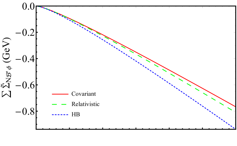
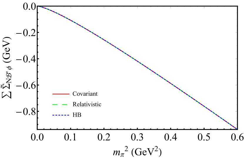
Figure 2: Sum of all FRR renormalized nucleon-baryon-meson self-energy contributions in different schemes. The upper figure compares the schemes at the same cutoff scale $\Lambda_{(\text{Cov})}=\Lambda_{(\text{Rel})}=\Lambda_{(\text{HB})}=0.8$ GeV. The bottom figure shows the fit of the relativistic schemes to the HB scheme at $\Lambda_{(\text{HB})}=0.8$ GeV. The fit parameters are shown in Table 1.

In Fig. 2 we show the sum of all FRR renormalized nucleon-baryon-meson self-energy contributions for each scheme. As we see in the top half, the relativistic schemes do differ at the 10-20% level when the same cut-off mass, 0.8 GeV, is used in all of them. However, as shown in the bottom half of Fig. 2, if we allow the values of the cutoff mass to vary with scheme, one finds excellent agreement between all three. The variation in $\Lambda$ is indeed somewhat subtle.

Since the cutoff scales $\Lambda_{(\text{Cov})}$ and $\Lambda_{(\text{Rel})}$, corresponding to the bottom half of Fig. 2, are quite close, as shown in Table 1, we set $\Lambda_{(\text{Cov})}=\Lambda_{(\text{Rel})}$ in the subsequent fits.

Table 1: Regulator mass and difference in unrenormalized coefficient of $m_{\pi}^{4}$ determined by fitting the corresponding self-energies calculated in the HB scheme (Eq. (25)), using $\Lambda_{(\text{HB})}\,=\,0.8$ GeV.

Scheme	Baryon	$\Lambda$ (GeV)	$d_{4}$ ($10^{-2}$ GeV-3 )
Covariant	Nucleon	1.05	0.69
	Lambda	1.15	8.82
	Sigma	0.93	-0.01
	Xi	1.04	2.74
Relativistic	Nucleon	1.01	6.78
	Lambda	1.06	9.79
	Sigma	0.91	2.38
	Xi	0.98	3.20

While we have considered one value of $\Lambda$ for the sum over intermediate baryons in this comparison, one may conduct a comparison on a diagram-by-diagram basis. In such a case, one could theoretically have different regulator cutoffs for each baryon-baryon-meson contribution. However, with the level of agreement seen above, it seems sufficient to only have one.

III.2 Fit Strategy

The fitting procedure is as follows. Firstly, we apply the FVCs of Sec. II.3 to the lattice results, taking them from finite to infinite volume.

Then, we fit the infinite volume results available at several quark masses and lattice spacings to function containing both the physics of chiral non-analytic behavior and a term linear in the square of the lattice spacing to address finite lattice spacing corrections at $\mathcal{O}(a^{2})$. For the nucleon, we have

$$M_{N}=\ C_{0}+C_{2}\,m_{\pi}^{2}+a_{4}\,m_{\pi}^{4}+\tilde{\Sigma}_{NN\pi}+\tilde{\Sigma}_{N\Lambda K}+\tilde{\Sigma}_{N\Sigma K}$$

$$+\tilde{\Sigma}_{NN\eta}+\tilde{\Sigma}_{N\Delta\pi}+\tilde{\Sigma}_{N\Sigma^{*}K}+\tilde{\Sigma}_{N\pi,\mathrm{tad}}+D_{a}\,a^{2}\,.$$ (26)

We note the PACS-CS results are obtained with a nonperturbatively improved Wilson-Clover fermion action such that the leading lattice artifact is the same as for the CLS results [2], and addressed at $\mathcal{O}(a^{2})$ by the final term in Eq. (III.2).

The fit parameters include $C_{0}$, $C_{2}$, $a_{4}$ and $D_{a}$. With the parameters constrained by lattice QCD results, one can then use Eq. (III.2) to interpolate/extrapolate to any value of $m_{\pi}^{2}$ or lattice spacing approaching the continuum limit. For example, one can expose the lattice spacing dependence of the lattice results by using Eq. (III.2) without the final term to access the physical quark masses and then plot the results as a function of $a^{2}$.

As a final step, we also explore the addition of the physical baryon mass to the data set and refit to obtain our best estimates of the low-energy coefficients.

In order to check the degree of model dependence associated with the three schemes under consideration, we compare our renormalized RSCs, $C_{0}$ and $C_{2}$ to the linear combinations of SU(2) LECs reported using $\chi$PT.

Finally, given the large uncertainty in the tadpole coefficient of Eq. (18), we consider the upper and lower bounds of this coefficient as a source of systematic uncertainty. We note that the upper limit of this coefficient corresponds to an absence of tadpole contributions.

III.3 Fit to PACS-CS lattice QCD data

Recent advances in computational capabilities and techniques have led to lattice QCD calculations near physical values of the light quark masses. Our aim in this section is compare analyses of the historical PACS-CS lattice QCD results [1], which extend over a wide range of pion mass, using the three schemes described. Note that, we choose to exclude two data points from the PACS-CS data set, one near the physical point with $m_{\pi}L\approx 2$, and one simulated with a different strange quark mass.

Table 2: Fits obtained from the PACS-CS nucleon mass lattice QCD results of Ref. [1], combined with the physical mass. The errors associated with the fit parameters are statistical followed by systematic as described in the text. The regulator cutoff for relativistic and HB formalisms are $\Lambda_{(\text{Cov})}=\Lambda_{(\text{Rel})}=1.0$ GeV and $\Lambda_{(\text{HB})}=0.8$ GeV respectively.

Scheme	$C_{0}$ (GeV)	$C_{2}$ (GeV-1)	$a_{4}$ (GeV-3)
Covariant	0.885(1)(5)	3.59(5)(37)	-0.17(10)(49)
Relativistic	0.882(1)(6)	3.69(7)(40)	0.25(13)(80)
HB	0.883(1)(5)	3.59(5)(35)	-0.06(9)(54)

In the case of the PACS-CS data set [1], we cannot readily calculate the $\mathcal{O}(a^{2})$ leading lattice artifact correction, because the lattice spacing is kept constant in the PACS-CS scheme. As an initial fit, we set $D_{a}=0$ in Eq. (III.2). The results of this initial fit are shown in Fig. 3 and Table 2.

We note that the uncertainty associated with the physical point is several orders of magnitude smaller than that of the lattice data, this means that the goodness of fit is primarily determined by the physical point. Therefore, to have some reasonable gauge of the goodness of fit, we exclude the physical point in the $\chi^{2}_{\text{dof}}$ calculation.

As seen in Fig. 3, the fits to the PACS-CS data are virtually indistinguishable. The $\chi^{2}_{\text{dof}}$ is approximately 0.26 for all three schemes.

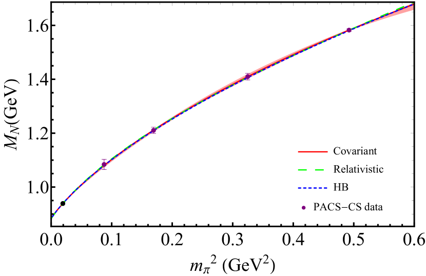
Figure 3: Fits to the PACS-CS nucleon mass data in the three schemes under consideration, covariant and relativistic formalisms at $\Lambda_{(\text{Cov})}=1.0$ GeV, and the heavy-baryon scheme at $\Lambda_{(\text{HB})}=0.8$ GeV. The physical nucleon mass (black point) is combined with the lattice results in constraining the fit parameters. The data points are finite volume corrected but there has been no correction applied for the finite lattice spacing as described in the text. The uncertainties on individual data points are statistical while the narrow extrapolation band incorporates both statistical and systematic uncertainties.

Not only are the fits to the data over values of $m_{\pi}^{2}\in 0.02-0.50$ GeV² using the three schemes extremely close but, as we see in Table 2, the renormalized RSCs $C_{0}$ and $C_{2}$ are also completely consistent. It is also necessary to examine if the value of $C_{2}$ is consistent with the input used in the coefficient of the tadpole contribution of Eq. (18). This is due to the fact that, in the nucleon mass expansion, the renormalized coefficient of the $m_{\pi}^{2}$ is related to one of the tadpole coefficients, specifically $C_{2}=-4c_{1}$. In obtaining the combination of Eq. (18), Refs.  [9, 91] quote $c_{1}=-0.9^{+0.5}_{-0.2}$ GeV^-1. Taking the average value of $C_{2}$ in Table 2, we find $c_{1}=-0.91(1)$ GeV^-1 (negligible difference when added in quadrature), which is completely consistent with the input.

In summary, contrary to claims in the literature, the use of HB theory with FRR does allow one to determine model independent low-energy coefficients using lattice data over a wide range of $m_{\pi}^{2}$.

Table 3: Renormalized RSCs obtained from fits to the PACS-CS octet baryon mass lattice QCD results [1], combined with the physical masses. The regulator cutoff masses for the relativistic and HB formalisms are $\Lambda_{(\text{Cov})}=\Lambda_{(\text{Rel})}=1.0$ GeV and $\Lambda_{(\text{HB})}=0.8$ GeV, respectively.

Baryon	Scheme	$C_{0}$ (GeV)	$C_{2}$ (GeV-1)	$a_{4}$ (GeV-3)
Lambda	Covariant	1.077(3)	2.21(11)	-0.78(22)
	Relativistic	1.076(3)	2.24(11)	-0.71(21)
	HB	1.076(3)	2.26(10)	-0.76(21)
Sigma	Covariant	1.157(3)	2.11(10)	-0.70(21)
	Relativistic	1.157(3)	2.11(10)	-0.65(20)
	HB	1.157(3)	2.08(10)	-0.74(21)
Xi	Covariant	1.289(6)	1.64(22)	-0.97(45)
	Relativistic	1.288(6)	1.65(22)	-0.95(45)
	HB	1.289(6)	1.62(20)	-0.94(42)

The PACS-CS data set further provides the masses for the other octet baryon (hyperon) masses. Since we restricted the study of the nucleon to dimension two LECs in SU(2), for the hyperons, we use a form analogous to Eq. (III.2), again omitting the $\mathcal{O}(a^{2})$ lattice artifact correction. We reiterate that $C_{i}$ and $a_{i}$ simply correspond to the coefficients of the chiral expansion of the baryon mass.

In Fig. 4 we see that the baryon mass expansion for the other octet baryons describes the data fairly well. While we only show the covariant fit, the other fits are indistinguishable, similar to those shown in Fig. 3. While not significant for the nucleon, the fact that the strange quark mass used in the PACS-CS simulations is a little large [92] is manifest in Fig. 4. There the extrapolation curves dip down to pass through the experimental values in a manner that leaves the lattice QCD results at the smallest pion mass included sitting above the curves. In Table 3 we see a similar trend to that found for the nucleon. With a cutoff mass chosen to give a good fit over the large range of $m_{\pi}^{2}$ provided by PACS-CS, there is very little difference in the renormalized coefficients $C_{0}$ and $C_{2}$. Recall that $a_{4}$ is not renormalized and therefore has no physical meaning.

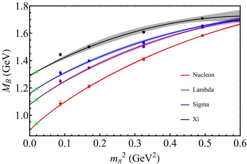
Figure 4: Fits to the PACS-CS octet baryon mass results in the covariant formalism at $\Lambda_{(\text{Cov})}=1.0$ GeV, with the inclusion of the physical points (green dots). The data points are finite volume corrected. The extrapolation bands and errors on individual data points are purely statistical.

IV Analysis of the latest CLS Lattice QCD results for the nucleon

Here, we focus on the most recent nucleon mass lattice QCD results from the CLS collaboration [2]. This data set is chosen because it presents a range of accurate lattice QCD results up to $m_{\pi}^{2}=0.14$ GeV², with the physical mass scale set using the modern gradient flow method [93].

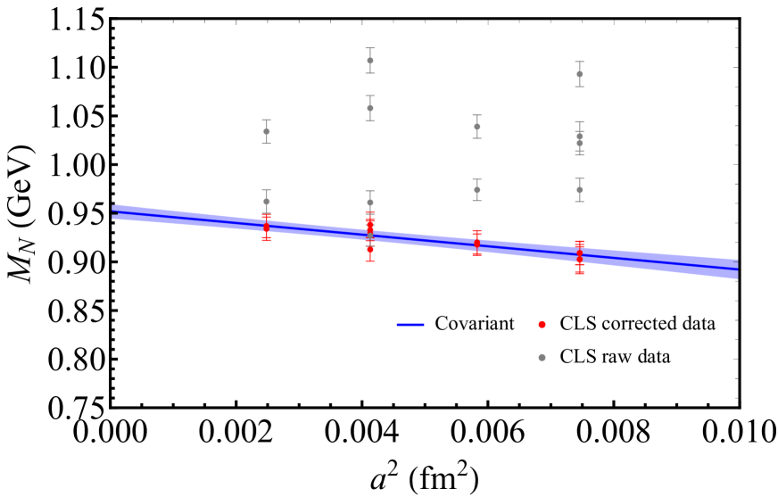
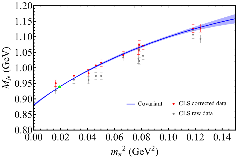
Figure 5: Fits to the CLS data set in the covariant formalism at $\Lambda_{(\text{Cov})}=1.0$ GeV. The top panel shows the uncorrected data at various pion masses along with a fit to the finite volume corrected data evaluated at $m_{\pi}^{2}=m_{\pi}^{2}|_{\text{phys}}$, where $D_{a}\approx-6$ GeV fm^-2. The bottom panel shows our fit to the CLS results in the continuum and infinite volume limit with the inclusion of the physical point (green dot). The uncertainties on individual data points are statistical while the extrapolation band incorporates both statistical and systematic uncertainties associated with the tadpole contribution.

Table 4: Fits including the physical point to the corrected CLS nucleon mass data [2]. The errors associated with the fit parameters are statistical followed by systematic as described in the text. The regulator cutoff for the covariant, relativistic, and HB formalisms are $\Lambda_{(\text{Cov})}=\Lambda_{(\text{Rel})}=1.0$ GeV and $\Lambda_{(\text{HB})}=0.8$ GeV respectively.

Scheme	$C_{0}$ (GeV)	$C_{2}$ (GeV-1)	$a_{4}$ (GeV-3)
Covariant	0.879(4)(2)	3.91(24)(20)	-3.2(20)(15)
Relativistic	0.878(4)(2)	3.97(24)(22)	-2.7(20)(20)
HB	0.878(4)(2)	3.92(24)(19)	-3.3(20)(15)

The results for the fits are shown in Fig. 5 and the renormalized RSCs are provided in Table 4. In performing the fits, we have omitted all data with $L<2.5$ fm in order to avoid large FVCs. We also show in Fig. 5 the lattice artifact correction, where $D_{a}\approx-6$ GeV fm^-2.

In the same way from the previous section, we perform a consistency check on $C_{2}$. We find, from Table 4, $C_{2}=-0.98(6)$ GeV^-1 which again is consistent with the input.

The $\chi^{2}_{\text{dof}}$ in all schemes are comparable at approximately 0.62. Again, all the fits are within one standard deviation of one another, and the differences are small.

In relation to the previous section, we also performed an analysis for the combined set of PACS-CS and CLS nucleon lattice data. For this particular case, we allow the coefficient of the tadpole, $\chi C$, to also be a fit parameter, constrained by Eq. (18). This is reasonable, as the wide range of $m_{\pi}^{2}$ covered by the PACS-CS data acts to restrict $\chi C$ in a meaningful manner. We use the CLS data to correct for the PACS-CS leading lattice artifact (noting that $D_{a}$ was set to zero for the PACS-CS data in the previous section). Since the variation in the lattice spacing for the PACS-CS data is small, the $\mathcal{O}(a^{2})$ correction simply shifts the data points by a constant amount. We find, for the renormalized RSCs and the coefficient of the tadpole, $C_{0}=0.884(4)$ GeV and $C_{2}=3.63(28)$ GeV^-1, and $\chi C=-1.6(10)$ GeV^-1, respectively. These values are consistent with the those found in the fits presented earlier.

V Comparison of the LECs and the $\bm{\sigma}$-term

V.1 Comparison of the LECs

Here, we wish to make a comparison between the $\chi$EFT renormalized series coefficients of the nucleon extracted using our three FRR schemes and those LECs obtained in earlier $\chi$PT work. In $\chi$PT, the chiral expansion of the nucleon mass in SU(2) is written as [94, 95, 78, 96]

$$M_{N}=m+k_{1}\,m_{\pi}^{2}+k_{2}\,m_{\pi}^{3}+k_{3}\,m_{\pi}^{4}\ln\frac{m_{\pi}}{\mu}+\cdots\,,$$ (27)

where $m$ is the renormalized nucleon mass in the chiral limit and the coefficients $k_{i}$ are linear combinations of the renormalized LECs. Explicitly, the $k_{i}$ are

$$k_{1}=-4c_{1},\mkern 20.0muk_{2}=-\frac{3g_{A}^{2}}{32\pi F^{2}},$$ (28)

and $k_{3}$ is provided in Eq. (17). $g_{A}$ and $F$ are the chiral limit values of the axial-vector coupling constant and pion decay constant respectively. In line with common practice we take them at the physical values $g_{A}=1.27$ and $F=f_{\phi}=93$ MeV.

We note that the values of $k_{3}$ found in the relativistic schemes are different from that found in the HB scheme. Clearly, in the limit $M_{N}\to\infty$, the term proportional to $g_{A}^{2}/M_{N}$ vanishes, and

$$\lim_{M_{N}\to\infty}\mathcal{A}=\frac{24}{25}g_{A}^{2}\frac{1}{\Delta_{\Delta N}}.$$ (29)

The total discrepancy in the coefficient of the NLNA term from the $NN\pi$ and the $N\Delta\pi$ self-energies amounts to 10% between the relativistic and HB formalisms. This difference, in comparison with the uncertainty associated with the tadpole coefficient, $\chi C$, is very small.

A comparison is shown in Table 5, where we present our (covariant) FRR result from the CLS data set Table 4 with earlier $\chi$PT works from Refs. [6] and [7]. These two works include the physical point constraint, but use a different regularization scheme, namely, infrared regularization (IR) and cut-off regularization (CR). The values for $k_{3}$ vary greatly with $\chi C$. With $\chi C$ in the range of Eq. (18), $k_{3}=1.62$ to 12.2 GeV^-3, while the values of Procura et al. [6] and Bernard et al. [7] yield $k_{3}=1.36\pm 3.29\ \text{GeV}^{-3}$ and $k_{3}=3.82\ \text{GeV}^{-3}$, respectively.

Table 5: Comparison of the renormalized series coefficients obtained using FRR in the covariant scheme to analyze the CLS data with those $\chi$PT LECs reported in Refs. [6] and [7]. Note in $\chi$PT notation $C_{0}=m$ and $C_{2}=k_{1}$.

Scheme	$C_{0}$ (GeV)	$C_{2}$ (GeV-1)
FRR result	0.879(4)(2)	3.91(24)(20)
Procura IR	0.883(3)	3.72(16)
Bernard CR	0.88	3.6 (fixed)

By way of comparison, we also show the results obtained from the CLS collaboration, by fitting a $\chi$PT-inspired form [2]

$$M_{N}(m_{\pi},a,L)=\mathring{M}_{N}+Bm_{\pi}^{2}+Cm_{\pi}^{3}+Da^{2}+E\frac{m_{\pi}^{3}}{m_{\pi}L}e^{-m_{\pi}L}\,.$$ (30)

$\mathring{M}_{N}$ is the nucleon mass in the chiral limit and the letters $B$-$E$ represent fit parameters including the LNA term. The lattice artifact correction and FVC are accounted for by the terms proportional to $D$ and $E$, respectively. Note that in our $\chi$EFT the LNA term is model- and scheme-independent and the coefficient is not a fit parameter. Nevertheless, with the above form, we obtain (including the physical point) $\mathring{M}_{N}=0.880(6)$ GeV, $B=3.75(46)$ GeV^-1, and $C=-4.8(13)$ GeV^-2. We remark that $C$ in this fit is roughly 14% smaller than the correct, model independent value, resulting in a shallow slope of the extrapolation curve near the physical point. Without the physical point constraint in the fit, one would find $C$ to be approximately 2 to 3 times smaller than the $\chi$EFT value. Any extrapolation relying on such a value is unphysical and extracting any physically meaningful observable is difficult. Alternatively, one may fix $C$ to $k_{2}$ of $\chi$EFT (see Eq. (28)), and in that case we find $\mathring{M}_{N}=0.875(1)$ GeV and $B=4.07(5)$ GeV^-1 producing reasonable agreement with the values quoted in Table 4.

V.2 The $\bm{\sigma}$-term

The pion-nucleon sigma term $\sigma_{\pi N}$ is defined as

$$\sigma_{\pi N}=\hat{m}\bra{N}\bar{u}u+\bar{d}d\ket{N}\,,$$ (31)

where $\hat{m}=(m_{u}+m_{d})/2$ with $m_{u}$ and $m_{d}$ being the light quark masses. From the quark mass dependence of the baryon and using the Feynman-Hellmann theorem, one can compute $\sigma_{\pi N}$ by

$$\sigma_{\pi N}=m_{\pi}^{2}\frac{\partial M_{N}}{\partial m_{\pi}^{2}}\,,$$ (32)

at the physical pion mass. The results for the application of Eq. (32) to each of the schemes summarized in Table 4 are presented in Table 6. The first set of uncertainties are statistical, while the second set are systematic, originating from the uncertainty in $\chi C$. The systematic uncertainty is determined by refitting to the CLS data using fixed values of $\chi C$ at the upper and lower bound given in Eq. (18), then calculating $\sigma_{\pi N}$ from the respective fits.

Table 6: Pion-nucleon sigma term at the physical point computed from the CLS data set using the fits for each scheme as summarized in Table 4. The first set of uncertainties are statistical and the second set are systematic.

Scheme	$\sigma_{\pi N}$ (MeV)
Covariant	$52.7\pm 3.1^{+0.7}_{-0.8}$
Relativistic	$53.2\pm 3.2^{+0.8}_{-0.9}$
HB	$53.0\pm 3.2^{+0.7}_{-0.8}$

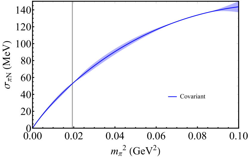
Figure 6: $\sigma_{\pi N}$ as a function of $m_{\pi}^{2}$ from the CLS data set fits of Table 4 in the covariant formalism at $\Lambda_{(\text{Cov})}=1.0$ GeV. The vertical line represents the physical value of $m_{\pi}^{2}$. The extrapolation band incorporates both statistical and systematic uncertainties.

We also show in Fig. 6 a plot of the $m_{\pi}^{2}$ dependence of $\sigma_{\pi N}$. Again, we show only the result in the covariant scheme, but the curves essentially overlap for the other two schemes, as in Fig. 3. Here, the gradient of the curve starts to flatten at around $m_{\pi}^{2}=0.1$ GeV², where the data points become sparse. With points available at larger $m_{\pi}^{2}$, as in the PACS-CS data set, we tend to see the curve flattening further out.

The explicit tadpole makes an important contribution to $\sigma_{\pi N}$ of order a few MeV. In exploring the systematic uncertainty associated with the tadpole contribution, we have observed a strong correlation between the coefficients $k_{1}$ and $k_{3}$ which act to reduce the effect of the systematic uncertainty. This results in a small net change in $\sigma_{\pi N}$.

In Table 7 we compare the value of $\sigma_{\pi N}$ calculated here with the values extracted by other methods. Deducing the value from pion-nucleon scattering data [97] may involve a number of complications [98]. As indicated, the preferred value seems to be around 58 MeV with an uncertainty of order 5 MeV [99]. This differs by a surprising amount from direct lattice calculations but is within the uncertainties of most applications of the Feynman-Hellmann theorem. The value found in our analysis, namely $53.0\pm 3.2^{+0.7}_{-0.8}$ MeV is clearly compatible with the value extracted from pion-nucleon scattering.

Table 7: Comparison with other determinations of the pion-nucleon sigma commutator.

Method	$\sigma_{\pi N}$ (MeV)	Ref.
$\pi N$ scattering	58(5)	[99]
Direct lattice calculation	45.9(7.4)(2.8)	[100]
	41.6(3.8)	[101]
Feynman-Hellmann + lattice data	45(6)	[16]
	52(3)(8)	[17]
	55(1)(4)	[18]
	44(3)(3)	[22]
This work	$53.0\pm 3.2^{+0.7}_{-0.8}$

VI Conclusion

We have presented a detailed study of the mass of the nucleon as a function of pion mass using finite range regularization to evaluate the self-energy integrals. The heavy baryon approximation is compared with a covariant scheme and a relativistic scheme. All three methods produce essentially identical fits to the lattice QCD results from the PACS-CS collaboration [1] over a wide range of pion mass, well beyond the power counting regime. The LECs derived from those fits are independent of the method used and agree well with those derived in earlier studies using $\chi$PT. A similar degree of model independence is found when the methods are applied to the other members of the nucleon octet.

These schemes were then applied to an analysis of the most recent data on the nucleon mass from the CLS Collaboration [2]. Of particular interest is the result that the values of $\sigma_{\pi N}$ extracted using all three methods, including the uncertainty in the coefficient of the (NLNA) $m_{\pi}^{4}\ln m_{\pi}$ term in the chiral expansion, are completely consistent. The result is $\sigma_{\pi N}=53.0\pm 3.2^{+0.7}_{-0.8}$ MeV. As illustrated in Table 7, this is in reasonable agreement with the value deduced from pion-nucleon scattering data as well as most applications of the Feynman-Hellmann theorem to lattice data.

Appendix A Effective SU(3)${}_{L}\times$SU(3)_R chiral Lagrangian

Beginning in the mesonic sector, $U$ is the 3$\times$3 unimodular unitary matrix which contains the meson fields $\phi$. In particular,

$$U=\exp\left(i\frac{\phi}{f_{\phi}}\right)=u^{2},$$ (33)

where

$$\phi=\sqrt{2}\begin{bmatrix}\frac{1}{\sqrt{2}}\pi^{0}+\frac{1}{\sqrt{6}}\eta&\pi^{+}&K^{+}\\ \pi^{-}&-\frac{1}{\sqrt{2}}\pi^{0}+\frac{1}{\sqrt{6}}\eta&K^{0}\\ K^{-}&\bar{K}^{0}&-\frac{2}{\sqrt{6}}\eta\end{bmatrix},$$ (34)

with $u$ the unitary square root of $U$. The investigations of the paper assumes the absence of an external field, so that the covariant derivative $D_{\mu}U\to\partial_{\mu}U$. The explicit chiral symmetry breaking is accounted for in the matrix $\chi=2B_{0}\mathcal{M}$ where $\mathcal{M}=\text{diag}(m_{u},m_{d},m_{s})$ and the parameter $B_{0}$ is related to the singlet quark condensate $3F_{0}^{2}B_{0}=-\left\langle 0|\bar{q}q|0\right\rangle_{0}$ with $F_{0}$ the pseudoscalar decay constant in the chiral limit.

In the octet baryon sector, each baryon field is a four-component Dirac field, and the matrix $B$ follows a similar structure to the meson matrix

$$B=\begin{bmatrix}\frac{1}{\sqrt{2}}\Sigma^{0}+\frac{1}{\sqrt{6}}\Lambda&\Sigma^{+}&p\\ \Sigma^{-}&-\frac{1}{\sqrt{2}}\Sigma^{0}+\frac{1}{\sqrt{6}}\Lambda&n\\ \Xi^{-}&\Xi^{0}&-\frac{2}{\sqrt{6}}\Lambda\end{bmatrix}.$$ (35)

The covariant derivative of the octet baryon is (again, in the absence of external fields) $D_{\mu}B=\partial_{\mu}+[\Gamma_{\mu},B]$, where $\Gamma_{\mu}\equiv\frac{1}{2}(u^{\dagger}\partial_{\mu}u+u\partial_{\mu}u^{\dagger})$. With a similar structure to the $\Gamma_{\mu}$, the baryon fields couple to the meson fields by the so-called chiral vielbein

$$u_{\mu}\equiv i(u^{\dagger}\partial_{\mu}u-u\partial_{\mu}u^{\dagger}),$$ (36)

which transforms as an axial-vector under parity transformation. In the NLO Lagrangian, additional chirally invariant structures are possible, and in particular we have $\chi_{+}=u^{\dagger}\chi u^{\dagger}+u\chi^{\dagger}u.$

In the decuplet baryon sector, the spin-3/2 decuplet fields are defined by the symmetric flavour tensor $T^{ijk}$ with

$$T^{111} =\Delta^{++}, T^{112} =\frac{1}{\sqrt{3}}\Delta^{+},$$

$$T^{122} =\frac{1}{\sqrt{3}}\Delta^{0}, T^{222} =\Delta^{-},$$

$$T^{113} =\frac{1}{\sqrt{3}}\Sigma^{*+}, T^{123} =\frac{1}{\sqrt{6}}\Sigma^{*0}, T^{223} =\frac{1}{\sqrt{3}}\Sigma^{*-},$$

$$T^{133} =\frac{1}{\sqrt{3}}\Xi^{*0}, T^{233} =\frac{1}{\sqrt{3}}\Xi^{*-}, T^{333} =\Omega^{-}.$$ (37)

The covariant derivative is defined by $D_{\mu}\left(T_{\nu}\right)^{ijk}=\partial_{\mu}\left(T_{\nu}\right)^{ijk}+\left(\Gamma_{\mu}\right)^{i}_{l}\left(T_{\nu}\right)^{ljk}+\left(\Gamma_{\mu}\right)^{j}_{l}\left(T_{\nu}\right)^{ilk}+\left(\Gamma_{\mu}\right)^{k}_{l}\left(T_{\nu}\right)^{ijl}$.

The propagators of the meson and octet baryon Lagrangian are the usual spin-0 and spin-1/2 Feynman propagators respectively, while the spin-3/2 propagator is a little bit more involved. Here, we simply quote the result [102]

$$S^{\mu\nu}_{F}(p) =-\frac{\not{p}+M_{T}}{p^{2}-M_{T}^{2}+i\varepsilon}\bigg{[}g^{\mu\nu}-\frac{1}{3}\gamma^{\mu}\gamma^{\nu}+\frac{(p^{\mu}\gamma^{\nu}-\gamma^{\mu}p^{\nu})}{3M_{T}}$$

$$-\frac{2}{3M_{T}^{2}}p^{\mu}p^{\nu}\bigg{]}+\frac{1}{3M_{T}^{2}}\frac{1+A}{1+2A}\bigg{[}\bigg{(}\frac{A}{1+2A}M_{T}$$

$$-\frac{1+A}{2(A+2A)}\not{p}\bigg{)}\gamma^{\mu}\gamma^{\nu}-\gamma^{\mu}p^{\nu}-\frac{A}{1+2A}p^{\mu}\gamma^{\nu}\bigg{)}\bigg{]}.$$ (38)

In addition, for the leading-order meson-octet-decuplet Lagnragian, the tensor $\Theta^{\mu\nu}$ is defined as

$$\Theta^{\mu\nu}\equiv g^{\mu\nu}+\frac{3A+1}{2}\gamma^{\mu}\gamma^{\nu},$$ (39)

where the choice of the off-shell parameter $A=-1$ simplifies both the propagator and the above tensor, as was done in Eq. (8).

Table 8: Squared coupling constants $C^{2}_{BB^{\prime}\phi}$ from two insertions of octet-octet-meson transition.

$N$		$\Lambda$		$\Sigma$		$\Xi$
$N\pi$	$\frac{3}{4}(D+F)^{2}$	$NK$	$\frac{1}{6}(D+3F)^{2}$	$NK$	$\frac{1}{2}(D-F)^{2}$	$\Lambda K$	$\frac{1}{12}(D-3F)^{2}$
$N\eta$	$\frac{1}{12}(D-3F)^{2}$	$\Lambda\eta$	$\frac{1}{3}D^{2}$	$\Lambda\pi$	$\frac{1}{3}D^{2}$	$\Sigma K$	$\frac{3}{4}(D+F)^{2}$
$\Lambda K$	$\frac{1}{12}(D+3F)^{2}$	$\Sigma\pi$	$D^{2}$	$\Sigma\pi$	$2F^{2}$	$\Xi\pi$	$\frac{3}{4}(D-F)^{2}$
$\Sigma K$	$\frac{3}{4}(D-F)^{2}$	$\Xi K$	$\frac{1}{6}(D-3F)^{2}$	$\Xi K$	$\frac{1}{2}(D+F)^{2}$	$\Xi\eta$	$\frac{1}{12}(D+3F)^{2}$

Table 9: Squared coupling constants $C^{2}_{BT^{\prime}\phi}$ from two insertions of octet-decuplet-meson transition.

$N$		$\Lambda$		$\Sigma$		$\Xi$
$\Delta\pi$	$\mathcal{C}^{2}$	$\Sigma^{*}\pi$	$\frac{3}{4}\mathcal{C}^{2}$	$\Delta K$	$\frac{2}{3}\mathcal{C}^{2}$	$\Sigma^{*}K$	$\frac{1}{4}\mathcal{C}^{2}$
$\Sigma^{*}K$	$\frac{1}{4}\mathcal{C}^{2}$	$\Xi^{*}K$	$\frac{1}{2}\mathcal{C}^{2}$	$\Sigma^{*}\pi$	$\frac{1}{6}\mathcal{C}^{2}$	$\Xi^{*}\pi$	$\frac{1}{4}\mathcal{C}^{2}$
				$\Sigma^{*}\eta$	$\frac{1}{4}\mathcal{C}^{2}$	$\Xi^{*}\eta$	$\frac{1}{4}\mathcal{C}^{2}$
				$\Xi^{*}K$	$\frac{1}{6}\mathcal{C}^{2}$	$\Omega K$	$\frac{1}{2}\mathcal{C}^{2}$

Appendix B Coupling constants of Lagrangian

Here, we present the coupling constants of the one-loop transitions given in the self-energy expressions Eqs. (7)-(9) determined from the effective Lagrangians Eqs. (II.1) and (II.1). These are presented in Tables 8 and 9. For the tadpole couplings, we primarily focus on the SU(2) limit, such that we only have

$$C_{N\pi,\text{tad}}=-3\left(-2c_{1}+\frac{c_{2}}{4}+c_{3}\right)m_{\pi}^{2}.$$ (40)

Appendix C Explicit self-energy contributions

In this section we explicitly show the closed form self-energy contributions in all schemes. We write the internal octet baryon mass as $M_{B^{\prime}}=M_{B}+\delta$ where $\delta$ is the mass difference between the internal and external octet baryons, and we divide the baryon-baryon-meson self-energy into 2 different parts: terms that produce analytic terms in $m_{\phi}^{2}$ and terms that produce non-analytic terms in $m_{\phi}^{2}$. Thus, we have, $\Sigma_{B\mathcal{B}^{\prime}\phi}=\Sigma_{B\mathcal{B}^{\prime}\phi}^{(1)}+\Sigma_{B\mathcal{B}^{\prime}\phi}^{(2)}$.

In FRR renormalization, the first part $\Sigma_{B\mathcal{B}^{\prime}\phi}^{(1)}$ is not generally of interest as they will be subtracted off. Here, we write down all the parts explicitly in all formalisms except for the relativistic formalism where $\Sigma_{B\mathcal{B}^{\prime}\phi}^{(1)}$ is lengthy and only will be partially presented.

$$\mkern-65.0mu\Sigma_{BB^{\prime}\phi}^{(\text{Cov},1)}= -\frac{C_{BB^{\prime}\phi}^{2}\Lambda^{6}\left(2M_{B}+\delta\right)}{96\pi^{2}f_{\phi}^{2}M_{B}(\Lambda^{2}-\delta^{2})\left(\Lambda^{2}-m_{\phi}^{2}\right)^{3}\left(\left(2M_{B}+\delta\right)^{2}-\Lambda^{2}\right)^{2}}\Bigg{\{}\Lambda^{2}\bigg{[}3\delta^{3}\left(2M_{B}+\delta\right)^{4}-\delta\Lambda^{2}\left(2M_{B}+\delta\right)^{2}\left(7\delta M_{B}+9M_{B}^{2}+6\delta^{2}\right)$$

$$+\Lambda^{4}\left(11\delta^{2}M_{B}+13\delta M_{B}^{2}-2M_{B}^{3}+3\delta^{3}\right)+2\Lambda^{6}M_{B}\bigg{]}$$

$$-m_{\phi}^{2}\Lambda^{2}\bigg{[}\delta\left(2M_{B}+\delta\right)^{2}\left(7\delta M_{B}+6M_{B}^{2}+3\delta^{2}\right)+2\Lambda^{2}\left(-4\delta^{2}M_{B}+\delta M_{B}^{2}+4M_{B}^{3}-3\delta^{3}\right)+\Lambda^{4}\left(M_{B}+3\delta\right)\bigg{]}$$

$$+m_{\phi}^{4}M_{B}\bigg{[}\delta\left(2M_{B}+\delta\right)^{2}\left(3M_{B}+2\delta\right)+\Lambda^{2}\left(13\delta M_{B}+10M_{B}^{2}+5\delta^{2}\right)-\Lambda^{4}\bigg{]}\Bigg{\}}$$

$$+\frac{C_{BB^{\prime}\phi}^{2}\Lambda^{8}\left(2M_{B}+\delta\right)^{2}\arctan\left(\frac{\sqrt{\left(\delta^{2}-\Lambda^{2}\right)\left(\Lambda^{2}-\left(2M_{B}+\delta\right)^{2}\right)}}{\delta\left(2M_{B}+\delta\right)+\Lambda^{2}}\right)}{32\pi^{2}f_{\phi}^{2}M_{B}^{3}\left(\Lambda^{2}-\delta^{2}\right)^{3/2}\left(\Lambda^{2}-m_{\phi}^{2}\right)^{4}\left(\left(2M_{B}+\delta\right)^{2}-\Lambda^{2}\right)^{5/2}}\Bigg{\{}\delta^{6}\left(2M_{B}+\delta\right)^{6}-2\delta^{4}\Lambda^{2}\left(2M_{B}+\delta\right)^{4}\left(3\delta M_{B}+3M_{B}^{2}+2\delta^{2}\right)$$

$$+6\delta^{2}\Lambda^{4}\left(2M_{B}+\delta\right)^{2}\left(3\delta^{3}M_{B}+4\delta^{2}M_{B}^{2}+2\delta M_{B}^{3}+M_{B}^{4}+\delta^{4}\right)+2\Lambda^{6}\left(-9\delta^{5}M_{B}-15\delta^{4}M_{B}^{2}-10\delta^{3}M_{B}^{3}+6\delta M_{B}^{5}+2M_{B}^{6}-2\delta^{6}\right)$$

$$+\Lambda^{8}\left(2\delta^{3}M_{B}-4\delta M_{B}^{3}-2M_{B}^{4}+\delta^{4}\right)-2m_{\phi}^{2}\bigg{[}\delta^{4}\left(2M_{B}+\delta\right)^{4}\left(3\delta M_{B}+3M_{B}^{2}+\delta^{2}\right)$$

$$-2\delta^{2}\Lambda^{2}\left(2M_{B}+\delta\right)^{2}\left(3\delta M_{B}+3M_{B}^{2}+\delta^{2}\right)\left(3\delta M_{B}+3M_{B}^{2}+2\delta^{2}\right)$$

$$+6\Lambda^{4}\left(3\delta M_{B}+3M_{B}^{2}+\delta^{2}\right)\left(3\delta^{3}M_{B}+4\delta^{2}M_{B}^{2}+2\delta M_{B}^{3}+M_{B}^{4}+\delta^{4}\right)-2\Lambda^{6}\left(\delta M_{B}+M_{B}^{2}+\delta^{2}\right)\left(5\delta M_{B}+5M_{B}^{2}+2\delta^{2}\right)$$

$$+\Lambda^{8}\left(\delta M_{B}+M_{B}^{2}+\delta^{2}\right)\bigg{]}+m_{\phi}^{4}\bigg{[}\delta^{2}\left(2M_{B}+\delta\right)^{2}\left(6\delta^{3}M_{B}+12\delta^{2}M_{B}^{2}+12\delta M_{B}^{3}+6M_{B}^{4}+\delta^{4}\right)$$

$$-2\Lambda^{2}\left(3\delta M_{B}+3M_{B}^{2}+2\delta^{2}\right)\left(6\delta^{3}M_{B}+12\delta^{2}M_{B}^{2}+12\delta M_{B}^{3}+6M_{B}^{4}+\delta^{4}\right)+6\Lambda^{4}\left(5\delta^{3}M_{B}+10\delta^{2}M_{B}^{2}+10\delta M_{B}^{3}+5M_{B}^{4}+\delta^{4}\right)$$

$$-2\Lambda^{6}\left(5\delta M_{B}+5M_{B}^{2}+2\delta^{2}\right)+\Lambda^{8}\bigg{]}+4m_{\phi}^{6}M_{B}^{3}\left(M_{B}+\delta\right)^{3}\Bigg{\}},$$ (41)

$$\mkern-55.0mu\Sigma_{BB^{\prime}\phi}^{(\text{Cov},2)} =\frac{C_{BB^{\prime}\phi}^{2}\Lambda^{8}\left(2M_{B}+\delta\right)}{64\pi^{2}f_{\phi}^{2}M_{B}\left(\Lambda^{2}-m_{\phi}^{2}\right)^{4}}\Bigg{\{}4\delta m_{\phi}^{2}\ln\left(\frac{m_{\phi}}{\Lambda}\right)+\frac{2(m_{\phi}^{2}-\delta^{2})(\delta+2M_{B})}{M_{B}^{2}}\bigg{[}(\delta\left(2M_{B}+\delta\right)-m_{\phi}^{2})\ln\left(\frac{m_{\phi}}{\Lambda}\right)$$

$$-\sqrt{(m_{\phi}^{2}-\delta^{2})((2M_{B}+\delta)^{2}-m_{\phi}^{2})}\arctan\left(\frac{\sqrt{(m_{\phi}^{2}-\delta^{2})((2M_{B}+\delta)^{2}-m_{\phi}^{2})}}{\delta\left(2M_{B}+\delta\right)+m_{\phi}^{2}}\right)\bigg{]}\Bigg{\}}.$$ (42)

In a similar fashion, we write $M_{T^{\prime}}=M_{B}+\Delta$ for the internal decuplet mass with $\Delta$ the mass difference between the external octet and internal decuplet baryon. Again, we divide the self-energies in two different terms.

$$\mkern-65.0mu\Sigma_{BT^{\prime}\phi}^{(\text{Cov},1)} =\frac{C_{BT^{\prime}\phi}^{2}\Lambda^{6}}{384\pi f_{\phi}^{2}M_{B}\left(M_{B}+\Delta\right)^{2}\left(\Lambda^{2}-\Delta^{2}\right)\left(\Lambda^{2}-m_{\phi}^{2}\right)^{3}}\Bigg{\{}$$

$$\Lambda^{2}\bigg{[}2\Lambda^{6}-2\Delta^{6}+4\Delta M_{B}\left(-3\Delta^{4}+\Delta^{2}\Lambda^{2}+\Lambda^{4}\right)+M_{B}^{2}\left(-24\Delta^{4}+13\Delta^{2}\Lambda^{2}+3\Lambda^{4}\right)-4M_{B}^{3}\left(4\Delta^{3}-3\Delta\Lambda^{2}\right)\bigg{]}$$

$$+\Lambda^{2}m_{\phi}^{2}\bigg{[}6\left(\Delta^{4}-\Lambda^{4}\right)+4M_{B}\left(5\Delta^{3}-3\Delta\Lambda^{2}\right)+M_{B}^{2}\left(25\Delta^{2}-9\Lambda^{2}\right)+8\Delta M_{B}^{3}\bigg{]}$$

$$-2m_{\phi}^{4}\bigg{[}3\Delta^{2}\Lambda^{2}-3\Lambda^{4}+2\Delta\Lambda^{2}M_{B}+4\Lambda^{2}M_{B}^{2}+2\Delta M_{B}^{3}\bigg{]}\Bigg{\}}$$

$$+\frac{C_{BT^{\prime}\phi}^{2}\Lambda^{8}}{192\pi^{2}f_{\phi}^{2}M_{B}^{3}\left(M_{B}+\Delta\right)^{2}}\Bigg{\{}\ln\left(\frac{M_{B}+\Delta}{\Lambda}\right)+\frac{\arctan\left(\frac{\sqrt{\left(\Delta^{2}-\Lambda^{2}\right)\left(\Lambda^{2}-\left(2M_{B}+\Delta\right)^{2}\right)}}{\Delta\left(2M_{B}+\Delta\right)+\Lambda^{2}}\right)}{\left(\Lambda^{2}-\Delta^{2}\right)^{3/2}\left(\Lambda^{2}-m_{\phi}^{2}\right)^{4}\sqrt{\left(2M_{B}+\Delta\right)^{2}-\Lambda^{2}}}\bigg{[}$$

$$-\Delta^{6}\left(2M_{B}+\Delta\right)^{6}+2\Delta^{4}\Lambda^{2}\left(2M_{B}+\Delta\right)^{4}\left(3\Delta M_{B}+3M_{B}^{2}+\Delta^{2}\right)-4\Lambda^{6}M_{B}^{3}\left(M_{B}+\Delta\right)^{3}$$

$$+\Lambda^{8}\left(2\Delta^{3}M_{B}-4\Delta M_{B}^{3}-2M_{B}^{4}+\Delta^{4}\right)-2\Lambda^{10}\left(\Delta M_{B}+M_{B}^{2}+\Delta^{2}\right)+\Lambda^{12}-2m_{\phi}^{2}\Big{(}-\Delta^{4}\left(2M_{B}+\Delta\right)^{4}\left(3\Delta M_{B}+3M_{B}^{2}+2\Delta^{2}\right)$$

$$+2\Delta^{2}\Lambda^{2}\left(2M_{B}+\Delta\right)^{2}\left(3\Delta M_{B}+3M_{B}^{2}+\Delta^{2}\right)\left(3\Delta M_{B}+3M_{B}^{2}+2\Delta^{2}\right)$$

$$-\Lambda^{4}\left(3\Delta M_{B}+3M_{B}^{2}+2\Delta^{2}\right)\left(6\Delta^{3}M_{B}+12\Delta^{2}M_{B}^{2}+12\Delta M_{B}^{3}+6M_{B}^{4}+\Delta^{4}\right)+2\Lambda^{6}\left(2\Delta^{3}M_{B}-4\Delta M_{B}^{3}-2M_{B}^{4}+\Delta^{4}\right)$$

$$-4\Lambda^{8}\left(\Delta M_{B}+M_{B}^{2}+\Delta^{2}\right)+2\Lambda^{10}\Big{)}+6m_{\phi}^{4}\Big{(}-\Delta^{2}\left(2M_{B}+\Delta\right)^{2}\left(3\Delta^{3}M_{B}+4\Delta^{2}M_{B}^{2}+2\Delta M_{B}^{3}+M_{B}^{4}+\Delta^{4}\right)$$

$$+2\Lambda^{2}\left(3\Delta M_{B}+3M_{B}^{2}+\Delta^{2}\right)\left(3\Delta^{3}M_{B}+4\Delta^{2}M_{B}^{2}+2\Delta M_{B}^{3}+M_{B}^{4}+\Delta^{4}\right)-\Lambda^{4}M_{B}\left(M_{B}+\Delta\right)\left(7\Delta M_{B}+7M_{B}^{2}+3\Delta^{2}\right)$$

$$-2\Lambda^{6}\left(\Delta M_{B}+M_{B}^{2}+\Delta^{2}\right)+\Lambda^{8}\Big{)}-2m_{\phi}^{6}\Big{(}-9\Delta^{5}M_{B}-15\Delta^{4}M_{B}^{2}-10\Delta^{3}M_{B}^{3}+6\Delta M_{B}^{5}+2M_{B}^{6}-2\Delta^{6}$$

$$+6\Lambda^{2}\left(3\Delta^{3}M_{B}+4\Delta^{2}M_{B}^{2}+2\Delta M_{B}^{3}+M_{B}^{4}+\Delta^{4}\right)-3\Lambda^{4}\left(3\Delta M_{B}+3M_{B}^{2}+2\Delta^{2}\right)+2\Lambda^{6}\Big{)}\bigg{]}\Bigg{\}},$$ (43)

$$\mkern-55.0mu\Sigma_{BT^{\prime}\phi}^{(\text{Cov},2)} =\frac{C_{BT^{\prime}\phi}^{2}\Lambda^{8}}{192\pi^{2}f_{\phi}^{2}M_{B}\left(M_{B}+\Delta\right)^{2}\left(\Lambda^{2}-m_{\phi}^{2}\right)^{4}}\Bigg{\{}2m_{\phi}^{2}\ln\left(\frac{m_{\phi}}{\Lambda}\right)\bigg{[}\Delta\left(2M_{B}+\Delta\right)^{3}+m_{\phi}^{2}\left(-6\Delta M_{B}-7M_{B}^{2}-2\Delta^{2}\right)+m_{\phi}^{4}\bigg{]}$$

$$+\frac{1}{M_{B}^{2}}\left(m_{\phi}^{2}-\Delta^{2}\right)\left((2M_{B}+\Delta)^{2}-m_{\phi}^{2}\right)^{2}\bigg{[}\ln\left(\frac{m_{\phi}}{\Lambda}\right)\left(\Delta\left(2M_{B}+\Delta\right)-m_{\phi}^{2}\right)$$

$$-\sqrt{(m_{\phi}^{2}-\Delta^{2})((2M_{B}+\Delta)^{2}-m_{\phi}^{2})}\arctan\left(\frac{\sqrt{(m_{\phi}^{2}-\Delta^{2})((2M_{B}+\Delta)^{2}-m_{\phi}^{2})}}{\Delta\left(2M_{B}+\Delta\right)+m_{\phi}^{2}}\right)\bigg{]}\Bigg{\}}.$$ (44)

The explicit nucleon-tadpole self-energy contribution in the covariant formalism is

$$\Sigma_{N\pi,\text{tad}}^{(\text{Cov})}=-\frac{\chi C\,\Lambda^{4}m_{\pi}^{2}}{32\pi^{2}f_{\pi}^{2}\left(\Lambda^{2}-m_{\pi}^{2}\right)^{4}}\left[2\Lambda^{6}+3\Lambda^{4}m_{\pi}^{2}-6\Lambda^{2}m_{\pi}^{4}+m_{\pi}^{6}+12\Lambda^{4}m_{\pi}^{2}\ln\left(\frac{m_{\pi}}{\Lambda}\right)\right].$$ (45)

As mentioned before, we present $\Sigma_{B\mathcal{B}^{\prime}\phi}^{(\text{Rel},1)}$ partially

$$\mkern-55.0mu\Sigma_{BB^{\prime}\phi}^{(\text{Rel},1)} =-\frac{C_{BB^{\prime}\phi}^{2}\Lambda^{3}\left(2M_{B}+\delta\right)^{2}\arctan\left(\frac{\sqrt{\left(M_{B}+\delta\right)^{2}-\Lambda^{2}}}{\Lambda}\right)}{64\pi^{2}f_{\phi}^{2}\left((M_{B}+\delta)^{2}-\Lambda^{2})\right)^{7/2}\left((m_{\phi}^{2}-\delta^{2})(m_{\phi}^{2}-(2M_{B}+\delta)^{2})+4\Lambda^{2}M_{B}^{2}\right)^{4}}\Bigg{\{}$$

$$\left(M_{B}+\delta\right)^{7}\left(\delta^{2}-m_{\phi}^{2}\right)^{4}\left((2M_{B}+\delta)^{2}-m_{\phi}^{2}\right)^{3}$$

$$+2\Lambda^{2}\left(M_{B}+\delta\right)^{5}\left(\delta^{2}-m_{\phi}^{2}\right)^{3}\left((2M_{B}+\delta)^{2}-m_{\phi}^{2}\right)^{2}\bigg{[}-3M_{B}^{2}\left(\delta^{2}-3m_{\phi}^{2}\right)-9\delta M_{B}\left(\delta^{2}-m_{\phi}^{2}\right)+12\delta M_{B}^{3}+6M_{B}^{4}-2\left(\delta^{2}-m_{\phi}^{2}\right)^{2}\bigg{]}$$

$$-4\Lambda^{4}\left(M_{B}+\delta\right)^{3}\left(\delta^{2}-m_{\phi}^{2}\right)^{2}\left((2M_{B}+\delta)^{2}-m_{\phi}^{2}\right)\bigg{[}M_{B}^{2}\left(13\delta^{2}-11m_{\phi}^{2}\right)+11\delta M_{B}\left(\delta^{2}-m_{\phi}^{2}\right)+4\delta M_{B}^{3}+2M_{B}^{4}+2\left(\delta^{2}-m_{\phi}^{2}\right)^{2}\bigg{]}$$

$$\times\bigg{[}2M_{B}^{2}\left(\delta^{2}+2m_{\phi}^{2}\right)-4\delta M_{B}\left(\delta^{2}-m_{\phi}^{2}\right)+12\delta M_{B}^{3}+6M_{B}^{4}-\left(\delta^{2}-m_{\phi}^{2}\right)^{2}\bigg{]}$$

$$+32\Lambda^{6}M_{B}^{2}\left(M_{B}+\delta\right)^{3}\left(\delta^{2}-m_{\phi}^{2}\right)\bigg{[}4\left(\delta^{2}-m_{\phi}^{2}\right)^{4}+38\delta M_{B}\left(\delta^{2}-m_{\phi}^{2}\right)^{3}+2M_{B}^{2}\left(63\delta^{2}-19m_{\phi}^{2}\right)\left(\delta^{2}-m_{\phi}^{2}\right)^{2}$$

$$+\delta M_{B}^{3}\left(\delta^{2}-m_{\phi}^{2}\right)\left(185\delta^{2}-176m_{\phi}^{2}\right)+M_{B}^{4}\left(141\delta^{4}-203\delta^{2}m_{\phi}^{2}+88m_{\phi}^{4}\right)+M_{B}^{5}\left(131\delta^{3}-27\delta m_{\phi}^{2}\right)+3M_{B}^{6}\left(55\delta^{2}-3m_{\phi}^{2}\right)$$

$$+104\delta M_{B}^{7}+26M_{B}^{8}\bigg{]}+64\Lambda^{8}M_{B}^{4}\left(M_{B}+\delta\right)^{3}\bigg{[}12\left(\delta^{2}-m_{\phi}^{2}\right)^{3}+31\delta M_{B}\left(\delta^{2}-m_{\phi}^{2}\right)^{2}-M_{B}^{2}\left(\delta^{2}-m_{\phi}^{2}\right)\left(19\delta^{2}+31m_{\phi}^{2}\right)$$

$$+2M_{B}^{3}\left(50\delta m_{\phi}^{2}-49\delta^{3}\right)+M_{B}^{4}\left(50m_{\phi}^{2}-44\delta^{2}\right)+6\delta M_{B}^{5}+2M_{B}^{6}\bigg{]}$$

$$-256\Lambda^{10}M_{B}^{5}\left(M_{B}+\delta\right)^{2}\bigg{[}M_{B}^{2}\left(22m_{\phi}^{2}-20\delta^{2}\right)-22\delta M_{B}\left(\delta^{2}-m_{\phi}^{2}\right)+4\delta M_{B}^{3}+2M_{B}^{4}-7\left(\delta^{2}-m_{\phi}^{2}\right)^{2}\bigg{]}$$

$$+512\Lambda^{12}M_{B}^{5}\bigg{[}2m_{\phi}^{2}\left(\delta M_{B}+M_{B}^{2}+\delta^{2}\right)-2\delta^{3}M_{B}+4\delta M_{B}^{3}+2M_{B}^{4}-\delta^{4}-m_{\phi}^{4}\bigg{]}\Bigg{\}}+\cdots,$$ (46)

$$\mkern-65.0mu\Sigma_{BB^{\prime}\phi}^{(\text{Rel},2)} =\frac{C_{BB^{\prime}\phi}^{2}\Lambda^{3}\left(2M_{B}+\delta\right)}{64\pi^{2}f_{\phi}^{2}\left((m_{\phi}^{2}-\delta^{2})(m_{\phi}^{2}-(2M_{B}+\delta)^{2})+4\Lambda^{2}M_{B}^{2}\right)^{4}}\Bigg{(}-512\Lambda^{5}M_{B}^{5}\arctan\left(\frac{\sqrt{(m_{\phi}^{2}-\delta^{2})((2M_{B}+\delta)^{2}-m_{\phi}^{2})}}{\delta\left(2M_{B}+\delta\right)+m_{\phi}^{2}}\right)$$

$$\times\left(2M_{B}+\delta\right)\left(m_{\phi}^{2}-\delta^{2}\right)^{3/2}\sqrt{(2M_{B}+\delta)^{2}-m_{\phi}^{2}}+\frac{1}{\left(m_{\phi}^{2}-\Lambda^{2}\right)^{7/2}}\arctan\left(\frac{\sqrt{m_{\phi}^{2}-\Lambda^{2}}}{\Lambda}\right)\bigg{\{}$$

$$-m_{\phi}^{8}\left(m_{\phi}^{2}-\delta^{2}\right)^{4}\left((2M_{B}+\delta)^{2}-m_{\phi}^{2}\right)^{3}$$

$$+2\Lambda^{2}m_{\phi}^{6}\left(m_{\phi}^{2}-\delta^{2}\right)^{3}\left((2M_{B}+\delta)^{2}-m_{\phi}^{2}\right)^{2}\bigg{[}6M_{B}^{2}\left(2\delta^{2}-3m_{\phi}^{2}\right)+9\delta M_{B}\left(\delta^{2}-m_{\phi}^{2}\right)+4\delta M_{B}^{3}+2\left(m_{\phi}^{2}-\delta^{2}\right)^{2}\bigg{]}$$

$$+4\Lambda^{4}m_{\phi}^{4}\left(m_{\phi}^{2}-\delta^{2}\right)^{2}\left(m_{\phi}^{2}-(2M_{B}+\delta)^{2}\right)\bigg{[}M_{B}^{2}\left(4\delta^{2}-10m_{\phi}^{2}\right)+4\delta M_{B}\left(\delta^{2}-m_{\phi}^{2}\right)+\left(m_{\phi}^{2}-\delta^{2}\right)^{2}\bigg{]}$$

$$\times\bigg{[}M_{B}^{2}\left(20\delta^{2}-18m_{\phi}^{2}\right)+11\delta M_{B}\left(\delta^{2}-m_{\phi}^{2}\right)+12\delta M_{B}^{3}+2\left(m_{\phi}^{2}-\delta^{2}\right)^{2}\bigg{]}$$

$$-32\Lambda^{6}M_{B}^{2}m_{\phi}^{4}\left(m_{\phi}^{2}-\delta^{2}\right)\bigg{[}4\left(m_{\phi}^{2}-\delta^{2}\right)^{4}+38\delta M_{B}\left(\delta^{2}-m_{\phi}^{2}\right)^{3}-8M_{B}^{2}\left(m_{\phi}^{2}-\delta^{2}\right)^{2}\left(7m_{\phi}^{2}-18\delta^{2}\right)$$

$$+\delta M_{B}^{3}\left(m_{\phi}^{2}-\delta^{2}\right)\left(263m_{\phi}^{2}-272\delta^{2}\right)+2M_{B}^{4}\left(128\delta^{4}-190\delta^{2}m_{\phi}^{2}+75m_{\phi}^{4}\right)+\left.M_{B}^{5}\left(96\delta^{3}-60\delta m_{\phi}^{2}\right)\right)\bigg{]}$$

$$+64\Lambda^{8}M_{B}^{4}m_{\phi}^{4}\bigg{[}M_{B}^{3}\left(70\delta m_{\phi}^{2}-68\delta^{3}\right)+31\delta M_{B}\left(m_{\phi}^{2}-\delta^{2}\right)^{2}+10M_{B}^{2}\left(m_{\phi}^{2}-\delta^{2}\right)\left(2\delta^{2}+3m_{\phi}^{2}\right)-12\left(m_{\phi}^{2}-\delta^{2}\right)^{3}\bigg{]}$$

$$-256\Lambda^{10}M_{B}^{5}m_{\phi}^{2}\bigg{[}M_{B}^{2}\left(30\delta m_{\phi}^{2}-28\delta^{3}\right)+M_{B}\left(-28\delta^{4}+34\delta^{2}m_{\phi}^{2}-6m_{\phi}^{4}\right)-7\delta\left(m_{\phi}^{2}-\delta^{2}\right)^{2}\bigg{]}$$

$$+512\Lambda^{12}M_{B}^{5}\bigg{[}M_{B}^{2}\left(6\delta m_{\phi}^{2}-4\delta^{3}\right)-2M_{B}\left(2\delta^{4}-3\delta^{2}m_{\phi}^{2}+m_{\phi}^{4}\right)-\delta\left(m_{\phi}^{2}-\delta^{2}\right)^{2}\bigg{]}\bigg{\}}\Bigg{)},$$ (47)

$$\mkern-55.0mu\Sigma_{BT^{\prime}\phi}^{(\text{Rel},1)} =-\frac{C_{BT^{\prime}\phi}^{2}\Lambda^{3}\arctan\left(\frac{\sqrt{\left(M_{B}+\Delta\right)^{2}-\Lambda^{2}}}{\Lambda}\right)}{96\pi^{2}f_{\phi}^{2}\left(M_{B}+\Delta\right)^{2}\left((M_{B}+\Delta)^{2}-\Lambda^{2})\right)^{7/2}\left((m_{\phi}^{2}-\Delta^{2})(m_{\phi}^{2}-(2M_{B}+\Delta)^{2})+4\Lambda^{2}M_{B}^{2}\right)^{4}}\Bigg{\{}$$

$$\left(M_{B}+\Delta\right)^{7}\left(m_{\phi}^{2}-\Delta^{2}\right)^{3}\left((2M_{B}+\Delta)^{2}-m_{\phi}^{2}\right)^{4}$$

$$-2\Lambda^{2}\left(M_{B}+\Delta\right)^{5}\left(m_{\phi}^{2}-\Delta^{2}\right)^{2}\left((2M_{B}+\Delta)^{2}-m_{\phi}^{2}\right)^{3}\bigg{[}-3\left(m_{\phi}^{2}-\Delta^{2}\right)^{2}+7\Delta M_{B}\left(m_{\phi}^{2}-\Delta^{2}\right)+M_{B}^{2}\left(11\Delta^{2}+7m_{\phi}^{2}\right)$$

$$+36\Delta M_{B}^{3}+18M_{B}^{4}\bigg{]}+24\Lambda^{4}M_{B}^{2}\left(M_{B}+\Delta\right)^{5}\left(\Delta^{2}-m_{\phi}^{2}\right)\left((2M_{B}+\Delta)^{2}-m_{\phi}^{2}\right)^{2}\bigg{[}3M_{B}^{2}\left(9\Delta^{2}-7m_{\phi}^{2}\right)+21\Delta M_{B}\left(\Delta^{2}-m_{\phi}^{2}\right)$$

$$+4\left(m_{\phi}^{2}-\Delta^{2}\right)^{2}+12\Delta M_{B}^{3}+6M_{B}^{4}\bigg{]}+16\Lambda^{6}M_{B}^{3}\left(M_{B}+\Delta\right)^{4}\left((2M_{B}+\Delta)^{2}-m_{\phi}^{2}\right)\bigg{[}35\left(m_{\phi}^{2}-\Delta^{2}\right)^{3}$$

$$-174\Delta M_{B}\left(m_{\phi}^{2}-\Delta^{2}\right)^{2}-6M_{B}^{2}\left(50\Delta^{4}-79\Delta^{2}m_{\phi}^{2}+29m_{\phi}^{4}\right)+4M_{B}^{3}\left(63\Delta m_{\phi}^{2}-62\Delta^{3}\right)+6M_{B}^{4}\left(21m_{\phi}^{2}-19\Delta^{2}\right)$$

$$+12\Delta M_{B}^{5}+4M_{B}^{6}\bigg{]}+64\Lambda^{8}M_{B}^{3}\left(M_{B}+\Delta\right)^{2}\bigg{[}-7\left(m_{\phi}^{2}-\Delta^{2}\right)^{4}+70\Delta M_{B}\left(m_{\phi}^{2}-\Delta^{2}\right)^{3}+70M_{B}^{2}\left(m_{\phi}^{2}-4\Delta^{2}\right)\left(m_{\phi}^{2}-\Delta^{2}\right)^{2}$$

$$-4M_{B}^{3}\left(146\Delta^{5}-251\Delta^{3}m_{\phi}^{2}+105\Delta m_{\phi}^{4}\right)+M_{B}^{4}\left(-688\Delta^{4}+912\Delta^{2}m_{\phi}^{2}-210m_{\phi}^{4}\right)+M_{B}^{5}\left(492\Delta m_{\phi}^{2}-436\Delta^{3}\right)$$

$$+4M_{B}^{6}\left(41m_{\phi}^{2}-20\Delta^{2}\right)+56\Delta M_{B}^{7}+14M_{B}^{8}\bigg{]}+128\Lambda^{10}M_{B}^{3}\bigg{[}-\left(m_{\phi}^{2}-\Delta^{2}\right)^{4}+10\Delta M_{B}\left(m_{\phi}^{2}-\Delta^{2}\right)^{3}$$

$$+10M_{B}^{2}\left(m_{\phi}^{2}-4\Delta^{2}\right)\left(m_{\phi}^{2}-\Delta^{2}\right)^{2}-20M_{B}^{3}\left(4\Delta^{5}-7\Delta^{3}m_{\phi}^{2}+3\Delta m_{\phi}^{4}\right)-10M_{B}^{4}\left(8\Delta^{4}-12\Delta^{2}m_{\phi}^{2}+3m_{\phi}^{4}\right)$$

$$+20M_{B}^{5}\left(3\Delta m_{\phi}^{2}-\Delta^{3}\right)+20M_{B}^{6}\left(2\Delta^{2}+m_{\phi}^{2}\right)+40\Delta M_{B}^{7}+10M_{B}^{8}\bigg{]}\Bigg{\}}+\cdots,$$ (48)

$$\mkern-65.0mu\Sigma_{BT^{\prime}\phi}^{(\text{Rel},2)} =\frac{C_{BT^{\prime}\phi}^{2}\Lambda^{5}M_{B}^{2}}{96\pi^{2}f_{\phi}^{2}\left(M_{B}+\Delta\right)^{2}\left((m_{\phi}^{2}-\Delta^{2})(m_{\phi}^{2}-(2M_{B}+\Delta)^{2})+4\Lambda^{2}M_{B}^{2}\right)^{4}}\Bigg{(}$$

$$-128\Lambda^{3}M_{B}^{3}\left(m_{\phi}^{2}-\Delta^{2}\right)^{3/2}\left((2M_{B}+\Delta)^{2}-m_{\phi}^{2}\right)^{5/2}\arctan\left(\frac{\sqrt{(m_{\phi}^{2}-\Delta^{2})((2M_{B}+\Delta)^{2}-m_{\phi}^{2})}}{\Delta\left(2M_{B}+\Delta\right)+m_{\phi}^{2}}\right)$$

$$-\frac{1}{\left(m_{\phi}^{2}-\Lambda^{2}\right)^{7/2}}\arctan\left(\frac{\sqrt{m_{\phi}^{2}-\Lambda^{2}}}{\Lambda}\right)\bigg{\{}\Delta m_{\phi}^{6}\left(m_{\phi}^{2}-\Delta^{2}\right)^{3}\left((2M_{B}+\Delta)^{2}-m_{\phi}^{2}\right)^{4}$$

$$+2\Lambda^{2}m_{\phi}^{4}\left(m_{\phi}^{2}-\Delta^{2}\right)^{2}\left((2M_{B}+\Delta)^{2}-m_{\phi}^{2}\right)^{3}\bigg{[}3\Delta\left(m_{\phi}^{2}-\Delta^{2}\right)^{2}+M_{B}\left(12\Delta^{4}-17\Delta^{2}m_{\phi}^{2}+5m_{\phi}^{4}\right)-6M_{B}^{2}\left(5\Delta m_{\phi}^{2}-2\Delta^{3}\right)\bigg{]}$$

$$-24\Lambda^{4}M_{B}^{2}m_{\phi}^{4}\left(m_{\phi}^{2}-\Delta^{2}\right)\left((2M_{B}+\Delta)^{2}-m_{\phi}^{2}\right)^{2}\bigg{[}4\Delta\left(m_{\phi}^{2}-\Delta^{2}\right)^{2}-M_{B}\left(-16\Delta^{4}+11\Delta^{2}m_{\phi}^{2}+5m_{\phi}^{4}\right)-2M_{B}^{2}\left(5\Delta m_{\phi}^{2}-8\Delta^{3}\right)\bigg{]}$$

$$+16\Lambda^{6}M_{B}^{3}m_{\phi}^{4}\bigg{[}-35\left(m_{\phi}^{2}-\Delta^{2}\right)^{4}+314\Delta M_{B}\left(m_{\phi}^{2}-\Delta^{2}\right)^{3}+2M_{B}^{2}\left(m_{\phi}^{2}-\Delta^{2}\right)^{2}\left(145m_{\phi}^{2}-556\Delta^{2}\right)$$

$$-4M_{B}^{3}\left(484\Delta^{5}-843\Delta^{3}m_{\phi}^{2}+359\Delta m_{\phi}^{4}\right)-8M_{B}^{4}\left(206\Delta^{4}-283\Delta^{2}m_{\phi}^{2}+75m_{\phi}^{4}\right)+16M_{B}^{5}\left(35\Delta m_{\phi}^{2}-34\Delta^{3}\right)\bigg{]}$$

$$-64\Lambda^{8}M_{B}^{3}m_{\phi}^{2}\bigg{[}-7\left(m_{\phi}^{2}-\Delta^{2}\right)^{4}+70\Delta M_{B}\left(m_{\phi}^{2}-\Delta^{2}\right)^{3}+70M_{B}^{2}\left(m_{\phi}^{2}-4\Delta^{2}\right)\left(m_{\phi}^{2}-\Delta^{2}\right)^{2}$$

$$-4M_{B}^{3}\left(140\Delta^{5}-239\Delta^{3}m_{\phi}^{2}+99\Delta m_{\phi}^{4}\right)-2M_{B}^{4}\left(280\Delta^{4}-372\Delta^{2}m_{\phi}^{2}+85m_{\phi}^{4}\right)+16M_{B}^{5}\left(15\Delta m_{\phi}^{2}-14\Delta^{3}\right)\bigg{]}$$

$$+128\Lambda^{10}M_{B}^{3}\bigg{[}-\left(m_{\phi}^{2}-\Delta^{2}\right)^{4}+10\Delta M_{B}\left(m_{\phi}^{2}-\Delta^{2}\right)^{3}+10M_{B}^{2}\left(m_{\phi}^{2}-4\Delta^{2}\right)\left(m_{\phi}^{2}-\Delta^{2}\right)^{2}-20M_{B}^{3}\left(4\Delta^{5}-7\Delta^{3}m_{\phi}^{2}+3\Delta m_{\phi}^{4}\right)$$

$$-10M_{B}^{4}\left(8\Delta^{4}-12\Delta^{2}m_{\phi}^{2}+3m_{\phi}^{4}\right)+16M_{B}^{5}\left(3\Delta m_{\phi}^{2}-2\Delta^{3}\right)\bigg{]}\bigg{\}}\Bigg{)},$$ (49)

$$\mkern-55.0mu\Sigma^{(\text{Rel})}_{N\pi,\text{tad}}=\frac{\chi C\,\Lambda^{3}m_{\pi}^{2}}{256\pi^{2}f_{\pi}^{2}\left(\Lambda^{2}-m_{\pi}^{2}\right)^{7/2}}\left[\Lambda\sqrt{\Lambda^{2}-m_{\pi}^{2}}\left(-8\Lambda^{4}-10\Lambda^{2}m_{\pi}^{2}+3m_{\pi}^{4}\right)+3m_{\pi}^{2}\left(8\Lambda^{4}-4\Lambda^{2}m_{\pi}^{2}+m_{\pi}^{4}\right)\text{artanh}\left(\frac{\sqrt{\Lambda^{2}-m_{\pi}^{2}}}{\Lambda}\right)\right].$$ (50)

Finally, in the HB scheme

$$\mkern-55.0mu\Sigma_{BB^{\prime}\phi}^{(\text{HB},1)} =-\frac{C_{BB^{\prime}\phi}^{2}\Lambda^{5}}{384\pi^{2}f_{\phi}^{2}\left(\delta^{2}+\Lambda^{2}-m_{\phi}^{2}\right)^{4}}\Bigg{\{}3\pi\left(\Lambda^{6}+9\Lambda^{4}\left(\delta^{2}-m_{\phi}^{2}\right)-9\Lambda^{2}\left(m_{\phi}^{2}-\delta^{2}\right)^{2}+\left(m_{\phi}^{2}-\delta^{2}\right)^{3}\right)$$

$$+\frac{48\delta\Lambda\left(\delta^{2}-m_{\phi}^{2}\right)^{2}\left(\delta^{2}+\Lambda^{2}-m_{\phi}^{2}\right)}{m_{\phi}^{2}-\Lambda^{2}}$$

$$+\frac{2\delta\Lambda\left(\delta^{2}+\Lambda^{2}-m_{\phi}^{2}\right)^{2}\left(-28\delta^{2}\Lambda^{4}+8\Lambda^{6}-\left(21\delta^{2}+67\Lambda^{2}\right)m_{\phi}^{4}+\left(64\delta^{2}\Lambda^{2}+38\Lambda^{4}\right)m_{\phi}^{2}+21m_{\phi}^{6}\right)}{\left(m_{\phi}^{2}-\Lambda^{2}\right)^{3}}\Bigg{\}},$$ (51)

$$\mkern-55.0mu\Sigma_{BB^{\prime}\phi}^{(\text{HB},2)} =\frac{C_{BB^{\prime}\phi}^{2}\Lambda^{8}}{64\pi^{2}f_{\phi}^{2}\left(\delta^{2}+\Lambda^{2}-m_{\phi}^{2}\right)^{4}}\Bigg{\{}8\left(m_{\phi}^{2}-\delta^{2}\right)^{3/2}\bigg{[}2\arctan\left(\frac{\delta}{\sqrt{m_{\phi}^{2}-\delta^{2}}}\right)-\pi\bigg{]}$$

$$-\frac{\delta}{\Lambda^{3}\left(\Lambda^{2}-m_{\phi}^{2}\right)^{7/2}}\text{artanh}\left(\frac{\sqrt{\Lambda^{2}-m_{\phi}^{2}}}{\Lambda}\right)\bigg{[}-16\delta^{2}\Lambda^{10}+8\Lambda^{8}\left(7\delta^{2}+3\Lambda^{2}\right)m_{\phi}^{2}+\left(6\delta^{6}\Lambda^{2}+24\delta^{4}\Lambda^{4}-34\delta^{2}\Lambda^{6}-60\Lambda^{8}\right)m_{\phi}^{4}$$

$$-\left(\delta^{6}+27\delta^{4}\Lambda^{2}+39\delta^{2}\Lambda^{4}-35\Lambda^{6}\right)m_{\phi}^{6}+3\left(\delta^{4}+12\delta^{2}\Lambda^{2}+5\Lambda^{4}\right)m_{\phi}^{8}-3\left(\delta^{2}+5\Lambda^{2}\right)m_{\phi}^{10}+m_{\phi}^{12}\bigg{]}\Bigg{\}}.$$ (52)

Then observing Eqs. (22) and (23), we note that the expression for the octet-decuplet-meson self-energy will be the same besides the factor of 2/3, and replacing $\delta\to\Delta$ and $C_{BB^{\prime}\phi}\to C_{BT^{\prime}\phi}$. We further remark that $\Sigma^{(\text{Rel})}_{N\pi,\text{tad}}=\Sigma^{(\text{HB})}_{N\pi,\text{tad}}$.

References

- Aoki et al. [2009] S. Aoki, K.-I. Ishikawa, N. Ishizuka, T. Izubuchi, D. Kadoh, K. Kanaya, Y. Kuramashi, Y. Namekawa, M. Okawa, Y. Taniguchi, A. Ukawa, N. Ukita, and T. Yoshié (PACS-CS Collaboration), flavor lattice QCD toward the physical point, Phys. Rev. D 79, 034503 (2009).
- Ottnad et al. [2023] K. Ottnad, D. Djukanovic, H. B. Meyer, G. von Hippel, and H. Wittig, Mass and isovector matrix elements of the nucleon at zero-momentum transfer, PoS LATTICE2022, 117 (2023), arXiv:2212.09940 [hep-lat] .
- Leinweber et al. [2000] D. B. Leinweber, A. W. Thomas, K. Tsushima, and S. V. Wright, Baryon masses from lattice QCD: Beyond the perturbative chiral regime, Phys. Rev. D 61, 074502 (2000), arXiv:hep-lat/9906027 .
- Young et al. [2003] R. D. Young, D. B. Leinweber, and A. W. Thomas, Convergence of chiral effective field theory, Prog. Part. Nucl. Phys. 50, 399 (2003), arXiv:hep-lat/0212031 .
- Leinweber et al. [2004] D. B. Leinweber, A. W. Thomas, and R. D. Young, Physical nucleon properties from lattice QCD, Phys. Rev. Lett. 92, 242002 (2004), arXiv:hep-lat/0302020 .
- Procura et al. [2004] M. Procura, T. R. Hemmert, and W. Weise, Nucleon mass, sigma term, and lattice QCD, Phys. Rev. D 69, 034505 (2004).
- Bernard et al. [2004] V. Bernard, T. R. Hemmert, and U.-G. Meißner, Cutoff schemes in chiral perturbation theory and the quark mass expansion of the nucleon mass, Nuclear Physics A 732, 149 (2004).
- Bernard et al. [2005] V. Bernard, T. R. Hemmert, and U.-G. Meißner, Chiral extrapolations and the covariant small scale expansion, Physics Letters B 622, 141 (2005).
- Meißner [2006] U.-G. Meißner, Quark mass dependence of baryon properties: Foundations and applications, Nuclear Physics B - Proceedings Supplements 153, 170 (2006), proceedings of the Workshop on Computational Hadron Physics.
- Goeke et al. [2006] K. Goeke, J. Ossmann, P. Schweitzer, and A. Silva, Pion mass dependence of the nucleon mass in the chiral quark soliton model, The European Physical Journal A - Hadrons and Nuclei 27, 77 (2006).
- Procura et al. [2006] M. Procura, B. U. Musch, T. Wollenweber, T. R. Hemmert, and W. Weise, Nucleon mass: From lattice QCD to the chiral limit, Phys. Rev. D 73, 114510 (2006).
- Armour et al. [2010] W. Armour, C. R. Allton, D. B. Leinweber, A. W. Thomas, and R. D. Young, An Analysis of the nucleon spectrum from lattice partially-quenched QCD, Nucl. Phys. A 840, 97 (2010), arXiv:0810.3432 [hep-lat] .
- Hall et al. [2010] J. M. M. Hall, D. B. Leinweber, and R. D. Young, Power Counting Regime of Chiral Effective Field Theory and Beyond, Phys. Rev. D 82, 034010 (2010), arXiv:1002.4924 [hep-lat] .
- Ren et al. [2012] X.-L. Ren, L. S. Geng, J. M. Camalich, J. Meng, and H. Toki, Octet baryon masses in next-to-next-to-next-to-leading order covariant baryon chiral perturbation theory, Journal of High Energy Physics 2012, 73 (2012).
- Bruns et al. [2013] P. C. Bruns, L. Greil, and A. Schäfer, Chiral extrapolation of baryon mass ratios, Phys. Rev. D 87, 054021 (2013), arXiv:1209.0980 [hep-ph] .
- Shanahan et al. [2013] P. E. Shanahan, A. W. Thomas, and R. D. Young, Sigma terms from an SU(3) chiral extrapolation, Phys. Rev. D 87, 074503 (2013), arXiv:1205.5365 [nucl-th] .
- Alvarez-Ruso et al. [2013] L. Alvarez-Ruso, T. Ledwig, J. Martin Camalich, and M. J. Vicente-Vacas, Nucleon mass and pion-nucleon sigma term from a chiral analysis of lattice QCD data, Phys. Rev. D 88, 054507 (2013), arXiv:1304.0483 [hep-ph] .
- Ren et al. [2015] X.-L. Ren, L.-S. Geng, and J. Meng, Scalar strangeness content of the nucleon and baryon sigma terms, Phys. Rev. D 91, 051502 (2015), arXiv:1404.4799 [hep-ph] .
- Lutz et al. [2018] M. F. M. Lutz, Y. Heo, and X.-Y. Guo, On the convergence of the chiral expansion for the baryon ground-state masses, Nucl. Phys. A 977, 146 (2018), arXiv:1801.06417 [hep-lat] .
- Bali et al. [2022] G. S. Bali, S. Collins, W. Söldner, and S. Weishäupl (RQCD Collaboration), Leading order mesonic and baryonic su(3) low energy constants from lattice QCD, Phys. Rev. D 105, 054516 (2022).
- Lutz et al. [2023] M. F. M. Lutz, Y. Heo, and X.-Y. Guo, Low-energy constants in the chiral Lagrangian with baryon octet and decuplet fields from Lattice QCD data on CLS ensembles, Eur. Phys. J. C 83, 440 (2023), arXiv:2301.06837 [hep-lat] .
- Copeland et al. [2023] P. M. Copeland, C.-R. Ji, and W. Melnitchouk, Octet and decuplet baryon terms and mass decompositions, Phys. Rev. D 107, 094041 (2023), arXiv:2112.03198 [nucl-th] .
- Leinweber [2004] D. B. Leinweber, Quark contributions to baryon magnetic moments in full, quenched and partially quenched QCD, Phys. Rev. D 69, 014005 (2004), arXiv:hep-lat/0211017 .
- Leinweber et al. [2005] D. B. Leinweber, S. Boinepalli, I. C. Cloet, A. W. Thomas, A. G. Williams, R. D. Young, J. M. Zanotti, and J. B. Zhang, Precise determination of the strangeness magnetic moment of the nucleon, Phys. Rev. Lett. 94, 212001 (2005), arXiv:hep-lat/0406002 .
- Leinweber et al. [2006] D. B. Leinweber, S. Boinepalli, A. W. Thomas, P. Wang, A. G. Williams, R. D. Young, J. M. Zanotti, and J. B. Zhang, Strange electric form-factor of the proton, Phys. Rev. Lett. 97, 022001 (2006), arXiv:hep-lat/0601025 .
- Hall et al. [2013a] J. M. M. Hall, D. B. Leinweber, B. J. Owen, and R. D. Young, Finite-volume corrections to charge radii, Phys. Lett. B 725, 101 (2013a), arXiv:1210.6124 [hep-lat] .
- Hall et al. [2013b] J. M. M. Hall, D. B. Leinweber, and R. D. Young, Chiral extrapolations for nucleon electric charge radii, Phys. Rev. D 88, 014504 (2013b), arXiv:1305.3984 [hep-lat] .
- Shanahan et al. [2014] P. E. Shanahan, A. W. Thomas, R. D. Young, J. M. Zanotti, R. Horsley, Y. Nakamura, D. Pleiter, P. E. L. Rakow, G. Schierholz, and H. Stüben (CSSM, QCDSF/UKQCD), Magnetic form factors of the octet baryons from lattice QCD and chiral extrapolation, Phys. Rev. D 89, 074511 (2014), arXiv:1401.5862 [hep-lat] .
- Hall et al. [2012] J. M. M. Hall, D. B. Leinweber, and R. D. Young, Chiral extrapolations for nucleon magnetic moments, Phys. Rev. D 85, 094502 (2012), arXiv:1201.6114 [hep-lat] .
- Hall et al. [2014] J. M. M. Hall, D. B. Leinweber, and R. D. Young, Finite-volume and partial quenching effects in the magnetic polarizability of the neutron, Phys. Rev. D 89, 054511 (2014), arXiv:1312.5781 [hep-lat] .
- Bignell et al. [2018] R. Bignell, J. Hall, W. Kamleh, D. Leinweber, and M. Burkardt, Neutron magnetic polarizability with Landau mode operators, Phys. Rev. D 98, 034504 (2018), arXiv:1804.06574 [hep-lat] .
- Bignell et al. [2020] R. Bignell, W. Kamleh, and D. Leinweber, Magnetic polarizability of the nucleon using a Laplacian mode projection, Phys. Rev. D 101, 094502 (2020), arXiv:2002.07915 [hep-lat] .
- Edwards et al. [2006] R. G. Edwards, G. T. Fleming, P. Hagler, J. W. Negele, K. Orginos, A. V. Pochinsky, D. B. Renner, D. G. Richards, and W. Schroers (LHPC), The Nucleon axial charge in full lattice QCD, Phys. Rev. Lett. 96, 052001 (2006), arXiv:hep-lat/0510062 .
- Horsley et al. [2014] R. Horsley, Y. Nakamura, A. Nobile, P. E. L. Rakow, G. Schierholz, and J. M. Zanotti, Nucleon axial charge and pion decay constant from two-flavor lattice QCD, Phys. Lett. B 732, 41 (2014), arXiv:1302.2233 [hep-lat] .
- Liang et al. [2017] J. Liang, Y.-B. Yang, K.-F. Liu, A. Alexandru, T. Draper, and R. S. Sufian, Lattice Calculation of Nucleon Isovector Axial Charge with Improved Currents, Phys. Rev. D 96, 034519 (2017), arXiv:1612.04388 [hep-lat] .
- Berkowitz et al. [2017] E. Berkowitz, D. Brantley, C. Bouchard, C. C. Chang, M. A. Clark, N. Garron, B. Joo, T. Kurth, C. Monahan, H. Monge-Camacho, A. Nicholson, K. Orginos, E. Rinaldi, P. Vranas, and A. Walker-Loud, An accurate calculation of the nucleon axial charge with lattice QCD (2017), arXiv:1704.01114 [hep-lat] .
- Lutz et al. [2020] M. F. M. Lutz, U. Sauerwein, and R. G. E. Timmermans, On the axial-vector form factor of the nucleon and chiral symmetry, Eur. Phys. J. C 80, 844 (2020), arXiv:2003.10158 [hep-lat] .
- Mahbub et al. [2012] M. S. Mahbub, W. Kamleh, D. B. Leinweber, P. J. Moran, and A. G. Williams (CSSM Lattice), Roper Resonance in 2+1 Flavor QCD, Phys. Lett. B 707, 389 (2012), arXiv:1011.5724 [hep-lat] .
- Edwards et al. [2011] R. G. Edwards, J. J. Dudek, D. G. Richards, and S. J. Wallace, Excited state baryon spectroscopy from lattice QCD, Phys. Rev. D 84, 074508 (2011), arXiv:1104.5152 [hep-ph] .
- Lang and Verduci [2013] C. B. Lang and V. Verduci, Scattering in the N negative parity channel in lattice QCD, Phys. Rev. D 87, 054502 (2013), arXiv:1212.5055 [hep-lat] .
- Mahbub et al. [2013] M. S. Mahbub, W. Kamleh, D. B. Leinweber, P. J. Moran, and A. G. Williams, Structure and Flow of the Nucleon Eigenstates in Lattice QCD, Phys. Rev. D 87, 094506 (2013), arXiv:1302.2987 [hep-lat] .
- Engel et al. [2013] G. P. Engel, C. B. Lang, D. Mohler, and A. Schäfer (BGR), QCD with Two Light Dynamical Chirally Improved Quarks: Baryons, Phys. Rev. D 87, 074504 (2013), arXiv:1301.4318 [hep-lat] .
- Hall et al. [2013c] J. M. M. Hall, A. C. P. Hsu, D. B. Leinweber, A. W. Thomas, and R. D. Young, Finite-volume matrix Hamiltonian model for a system, Phys. Rev. D 87, 094510 (2013c), arXiv:1303.4157 [hep-lat] .
- Roberts et al. [2013] D. S. Roberts, W. Kamleh, and D. B. Leinweber, Wave Function of the Roper from Lattice QCD, Phys. Lett. B 725, 164 (2013), arXiv:1304.0325 [hep-lat] .
- Roberts et al. [2014] D. S. Roberts, W. Kamleh, and D. B. Leinweber, Nucleon Excited State Wave Functions from Lattice QCD, Phys. Rev. D 89, 074501 (2014), arXiv:1311.6626 [hep-lat] .
- Alexandrou et al. [2015] C. Alexandrou, T. Leontiou, C. N. Papanicolas, and E. Stiliaris, Novel analysis method for excited states in lattice QCD: The nucleon case, Phys. Rev. D 91, 014506 (2015), arXiv:1411.6765 [hep-lat] .
- Liu et al. [2016] Z.-W. Liu, W. Kamleh, D. B. Leinweber, F. M. Stokes, A. W. Thomas, and J.-J. Wu, Hamiltonian effective field theory study of the resonance in lattice QCD, Phys. Rev. Lett. 116, 082004 (2016), arXiv:1512.00140 [hep-lat] .
- Kiratidis et al. [2015] A. L. Kiratidis, W. Kamleh, D. B. Leinweber, and B. J. Owen, Lattice baryon spectroscopy with multi-particle interpolators, Phys. Rev. D 91, 094509 (2015), arXiv:1501.07667 [hep-lat] .
- Leinweber et al. [2016] D. Leinweber, W. Kamleh, A. Kiratidis, Z.-W. Liu, S. Mahbub, D. Roberts, F. Stokes, A. W. Thomas, and J. Wu, N* Spectroscopy from Lattice QCD: The Roper Explained, JPS Conf. Proc. 10, 010011 (2016), arXiv:1511.09146 [hep-lat] .
- Stokes et al. [2015] F. M. Stokes, W. Kamleh, D. B. Leinweber, M. S. Mahbub, B. J. Menadue, and B. J. Owen, Parity-expanded variational analysis for nonzero momentum, Phys. Rev. D 92, 114506 (2015), arXiv:1302.4152 [hep-lat] .
- Kiratidis et al. [2017] A. L. Kiratidis, W. Kamleh, D. B. Leinweber, Z.-W. Liu, F. M. Stokes, and A. W. Thomas, Search for low-lying lattice QCD eigenstates in the Roper regime, Phys. Rev. D 95, 074507 (2017), arXiv:1608.03051 [hep-lat] .
- Liu et al. [2017] Z.-W. Liu, W. Kamleh, D. B. Leinweber, F. M. Stokes, A. W. Thomas, and J.-J. Wu, Hamiltonian effective field theory study of the resonance in lattice QCD, Phys. Rev. D 95, 034034 (2017), arXiv:1607.04536 [nucl-th] .
- Wu et al. [2017] J.-J. Wu, H. Kamano, T. S. H. Lee, D. B. Leinweber, and A. W. Thomas, Nucleon resonance structure in the finite volume of lattice QCD, Phys. Rev. D 95, 114507 (2017), arXiv:1611.05970 [hep-lat] .
- Lang et al. [2017] C. B. Lang, L. Leskovec, M. Padmanath, and S. Prelovsek, Pion-nucleon scattering in the Roper channel from lattice QCD, Phys. Rev. D 95, 014510 (2017), arXiv:1610.01422 [hep-lat] .
- Wu et al. [2018] J.-j. Wu, D. B. Leinweber, Z.-w. Liu, and A. W. Thomas, Structure of the Roper Resonance from Lattice QCD Constraints, Phys. Rev. D 97, 094509 (2018), arXiv:1703.10715 [nucl-th] .
- Andersen et al. [2018] C. W. Andersen, J. Bulava, B. Hörz, and C. Morningstar, Elastic -wave nucleon-pion scattering amplitude and the (1232) resonance from Nf=2+1 lattice QCD, Phys. Rev. D 97, 014506 (2018), arXiv:1710.01557 [hep-lat] .
- Stokes et al. [2020] F. M. Stokes, W. Kamleh, and D. B. Leinweber, Elastic Form Factors of Nucleon Excitations in Lattice QCD, Phys. Rev. D 102, 014507 (2020), arXiv:1907.00177 [hep-lat] .
- Stokes et al. [2019] F. M. Stokes, W. Kamleh, and D. B. Leinweber, Structure and transitions of nucleon excitations via parity-expanded variational analysis, PoS LATTICE2019, 182 (2019), arXiv:2001.07919 [hep-lat] .
- Virgili et al. [2020] A. Virgili, W. Kamleh, and D. Leinweber, Role of chiral symmetry in the nucleon excitation spectrum, Phys. Rev. D 101, 074504 (2020), arXiv:1910.13782 [hep-lat] .
- Khan et al. [2021] T. Khan, D. Richards, and F. Winter, Positive-parity baryon spectrum and the role of hybrid baryons, Phys. Rev. D 104, 034503 (2021), arXiv:2010.03052 [hep-lat] .
- Morningstar et al. [2022] C. Morningstar, J. Bulava, A. D. Hanlon, B. Hörz, D. Mohler, A. Nicholson, S. Skinner, and A. Walker-Loud, Progress on Meson-Baryon Scattering, PoS LATTICE2021, 170 (2022), arXiv:2111.07755 [hep-lat] .
- Abell et al. [2022] C. D. Abell, D. B. Leinweber, A. W. Thomas, and J.-J. Wu, Regularization in nonperturbative extensions of effective field theory, Phys. Rev. D 106, 034506 (2022), arXiv:2110.14113 [hep-lat] .
- Bulava et al. [2023a] J. Bulava, A. D. Hanlon, B. Hörz, C. Morningstar, A. Nicholson, F. Romero-López, S. Skinner, P. Vranas, and A. Walker-Loud, Elastic nucleon-pion scattering at m=200 MeV from lattice QCD, Nucl. Phys. B 987, 116105 (2023a), arXiv:2208.03867 [hep-lat] .
- Bulava et al. [2023b] J. Bulava et al., Low-lying baryon resonances from lattice QCD (2023) arXiv:2310.08375 [hep-lat] .
- Abell et al. [2023a] C. D. Abell, D. B. Leinweber, A. W. Thomas, and J.-J. Wu, Effects of multiple single-particle basis states in scattering systems (2023a), arXiv:2305.18790 [nucl-th] .
- Abell et al. [2023b] C. D. Abell, D. B. Leinweber, Z.-W. Liu, A. W. Thomas, and J.-J. Wu, Low-lying odd-parity nucleon resonances as quark-model like states (2023b), arXiv:2306.00337 [hep-lat] .
- Wang and Thomas [2010] P. Wang and A. W. Thomas, The First Moments of Nucleon Generalized Parton Distributions, Phys. Rev. D 81, 114015 (2010), arXiv:1003.0957 [hep-ph] .
- Scapellato et al. [2022] A. Scapellato, C. Alexandrou, K. Cichy, M. Constantinou, K. Hadjiyiannakou, K. Jansen, and F. Steffens, Generalized parton distributions of the proton from lattice QCD, PoS LATTICE2021, 129 (2022), arXiv:2111.03226 [hep-lat] .
- He et al. [2022] F. He, C.-R. Ji, W. Melnitchouk, A. W. Thomas, and P. Wang, Generalized parton distributions of sea quarks in the proton from nonlocal chiral effective theory, Phys. Rev. D 106, 054006 (2022), arXiv:2202.00266 [hep-ph] .
- Lin [2023] H.-W. Lin, Pion valence-quark generalized parton distribution at physical pion mass, Phys. Lett. B 846, 138181 (2023).
- Copeland et al. [2021] P. M. Copeland, C.-R. Ji, and W. Melnitchouk, Octet and decuplet baryon self-energies in relativistic su(3) chiral effective theory, Phys. Rev. D 103, 094019 (2021).
- Jenkins and Manohar [1991] E. Jenkins and A. V. Manohar, Chiral corrections to the baryon axial currents, Physics Letters B 259, 353 (1991).
- Lutz and Kolomeitsev [2002] M. Lutz and E. Kolomeitsev, Relativistic chiral su(3) symmetry, large-nc sum rules and meson–baryon scattering, Nuclear Physics A 700, 193 (2002).
- Ledwig et al. [2014] T. Ledwig, J. M. Camalich, L. S. Geng, and M. J. V. Vacas, Octet-baryon axial-vector charges and su(3)-breaking effects in the semileptonic hyperon decays, Phys. Rev. D 90, 054502 (2014).
- Oller et al. [2006] J. A. Oller, M. Verbeni, and J. Prades, Meson-baryon effective chiral lagrangians to , Journal of High Energy Physics 2006, 079 (2006).
- Gasser et al. [1988] J. Gasser, M. Sainio, and A. Švarc, Nucleons with chiral loops, Nuclear Physics B 307, 779 (1988).
- Fettes et al. [2000] N. Fettes, U.-G. Meißner, M. Mojžiš, and S. Steininger, The chiral effective pion-nucleon lagrangian of order p4, Annals of Physics 283, 273 (2000).
- Fuchs et al. [2003] T. Fuchs, J. Gegelia, G. Japaridze, and S. Scherer, Renormalization of relativistic baryon chiral perturbation theory and power counting, Phys. Rev. D 68, 056005 (2003).
- Armstrong and McKeown [2012] D. S. Armstrong and R. D. McKeown, Parity-Violating Electron Scattering and the Electric and Magnetic Strange Form Factors of the Nucleon, Ann. Rev. Nucl. Part. Sci. 62, 337 (2012), arXiv:1207.5238 [nucl-ex] .
- Aniol et al. [1999] K. A. Aniol et al. (HAPPEX), Measurement of the neutral weak form-factors of the proton, Phys. Rev. Lett. 82, 1096 (1999), arXiv:nucl-ex/9810012 .
- Androic et al. [2010] D. Androic et al. (G0), Strange Quark Contributions to Parity-Violating Asymmetries in the Backward Angle G0 Electron Scattering Experiment, Phys. Rev. Lett. 104, 012001 (2010), arXiv:0909.5107 [nucl-ex] .
- Thomas [1983] A. W. Thomas, A Limit on the Pionic Component of the Nucleon Through SU(3) Flavor Breaking in the Sea, Phys. Lett. B 126, 97 (1983).
- Thomas [1984] A. W. Thomas, Chiral Symmetry and the Bag Model: A New Starting Point for Nuclear Physics, Adv. Nucl. Phys. 13, 1 (1984).
- Thomas [2003] A. W. Thomas, Chiral extrapolation of hadronic observables, Nucl. Phys. B Proc. Suppl. 119, 50 (2003), arXiv:hep-lat/0208023 .
- Donoghue et al. [1999] J. F. Donoghue, B. R. Holstein, and B. Borasoy, SU(3) baryon chiral perturbation theory and long distance regularization, Phys. Rev. D 59, 036002 (1999), arXiv:hep-ph/9804281 .
- Hall et al. [2011] J. M. M. Hall, F. X. Lee, D. B. Leinweber, K. F. Liu, N. Mathur, R. D. Young, and J. B. Zhang, Chiral extrapolation beyond the power-counting regime, Phys. Rev. D 84, 114011 (2011), arXiv:1101.4411 [hep-lat] .
- McGovern and Birse [2006] J. A. McGovern and M. C. Birse, Convergence of the chiral expansion for the nucleon mass, Phys. Rev. D 74, 097501 (2006), arXiv:hep-lat/0608002 .
- Alarcon et al. [2011] J. M. Alarcon, J. Martin Camalich, J. A. Oller, and L. Alvarez-Ruso, scattering in relativistic baryon chiral perturbation theory revisited, Phys. Rev. C 83, 055205 (2011), [Erratum: Phys.Rev.C 87, 059901 (2013)], arXiv:1102.1537 [nucl-th] .
- Frink et al. [2005] M. Frink, U.-G. Meissner, and I. Scheller, Baryon masses, chiral extrapolations, and all that, Eur. Phys. J. A 24, 395 (2005), arXiv:hep-lat/0501024 .
- Djukanovic et al. [2005] D. Djukanovic, M. R. Schindler, J. Gegelia, and S. Scherer, Improving the ultraviolet behavior in baryon chiral perturbation theory, Phys. Rev. D 72, 045002 (2005).
- Frink and Meißner [2004] M. Frink and U.-G. Meißner, Chiral extrapolations of baryon masses for unquenched three-flavor lattice simulations, Journal of High Energy Physics 2004, 028 (2004).
- Menadue et al. [2012] B. J. Menadue, W. Kamleh, D. B. Leinweber, and M. S. Mahbub, Isolating the in Lattice QCD, Phys. Rev. Lett. 108, 112001 (2012), arXiv:1109.6716 [hep-lat] .
- Lüscher [2010] M. Lüscher, Properties and uses of the wilson flow in lattice QCD, Journal of High Energy Physics 2010, 71 (2010).
- Steininger et al. [1998] S. Steininger, U.-G. Meißner, and N. Fettes, On wave function renormalization and related aspects in heavy fermion effective field theories, Journal of High Energy Physics 1998, 008 (1998).
- Becher and Leutwyler [1999] T. Becher and H. Leutwyler, Baryon chiral perturbation theory in manifestly lorentz invariant form, The European Physical Journal C - Particles and Fields 9, 643 (1999).
- Schindler et al. [2007] M. R. Schindler, D. Djukanovic, J. Gegelia, and S. Scherer, Chiral expansion of the nucleon mass to order , Physics Letters B 649, 390 (2007).
- Alarcón et al. [2012] J. M. Alarcón, J. M. Camalich, and J. A. Oller, Chiral representation of the scattering amplitude and the pion-nucleon sigma term, Phys. Rev. D 85, 051503 (2012).
- Ericson [1987] T. E. O. Ericson, A New Interpretation of the - Term, Phys. Lett. B 195, 116 (1987).
- Ruiz de Elvira et al. [2018] J. Ruiz de Elvira, M. Hoferichter, B. Kubis, and U.-G. Meißner, Extracting the -term from low-energy pion-nucleon scattering, J. Phys. G 45, 024001 (2018), arXiv:1706.01465 [hep-ph] .
- Yang et al. [2016] Y.-B. Yang, A. Alexandru, T. Draper, J. Liang, and K.-F. Liu (xQCD), and strangeness sigma terms at the physical point with chiral fermions, Phys. Rev. D 94, 054503 (2016), arXiv:1511.09089 [hep-lat] .
- Alexandrou et al. [2020] C. Alexandrou, S. Bacchio, M. Constantinou, J. Finkenrath, K. Hadjiyiannakou, K. Jansen, G. Koutsou, and A. Vaquero Aviles-Casco, Nucleon axial, tensor, and scalar charges and -terms in lattice QCD, Phys. Rev. D 102, 054517 (2020), arXiv:1909.00485 [hep-lat] .
- Scherer and Schindler [2011] S. Scherer and M. R. Schindler, A primer for chiral perturbation theory, Vol. 830 (Springer Science & Business Media, 2011).