Abstract

Entropy maximization and free energy minimization are general physical principles for modeling the dynamics of various physical systems. Notable examples include modeling decision-making within the brain using the free-energy principle, optimizing the accuracy-complexity trade-off when accessing hidden variables with the information bottleneck principle (Tishby et al., 2000), and navigation in random environments using information maximization (Vergassola et al., 2007). Built on this principle, we propose a new class of bandit algorithms that maximize an approximation to the information of a key variable within the system. To this end, we develop an approximated analytical physics-based representation of an entropy to forecast the information gain of each action and greedily choose the one with the largest information gain. This method yields strong performances in classical bandit settings. Motivated by its empirical success, we prove its asymptotic optimality for the two-armed bandit problem with Gaussian rewards. Owing to its ability to encompass the system’s properties in a global physical functional, this approach can be efficiently adapted to more complex bandit settings, calling for further investigation of information maximization approaches for multi-armed bandit problems.

1 Introduction

Multi-armed bandit problems have raised a vast interest in the past decades. They embody the challenge of balancing exploration and exploitation and have been applied to various different settings such as online recommendation (Bresler et al., 2014), medical trials (Thompson, 1933), dynamic pricing (Den Boer, 2015), and reinforcement learning-based decision making (Silver et al., 2016; Ryzhov et al., 2012). Besides the classic stochastic version of the multi-armed bandit problem, many subsequent extensions have been developed, providing finer models for specific applications. These extensions include linear bandits (Li et al., 2010), many-armed bandits (Bayati et al., 2020), and pure exploration problems such as thresholding bandits (Locatelli et al., 2016) or top-K bandits (Kalyanakrishnan et al., 2012; Kaufmann et al., 2016).

In the classic setting, an agent chooses an arm at each time step and observes a stochastic reward. Since they only observe the payoff of the chosen arm, the agent should regularly explore suboptimal arms. This is often referred as the exploration-exploitation trade-off. An agent can exploit its current knowledge to optimize gains by drawing the current empirically best arm or exploring other arms to potentially increase future gains.

In the infinite horizon setting, optimal strategies are characterized asymptotically by the Lai and Robbins bound (Lai et al., 1985). Among them, upper confidence bound (UCB, Auer (2000); Garivier and Cappé (2011)) methods associate a tuned confidence index to each arm, Thompson sampling (Kaufmann et al., 2012a; Agrawal and Goyal, 2013) relies on sampling the action from the posterior distribution that maximizes the expected reward, and deterministic minimum empirical divergence (DMED) (Honda and Takemura, 2010) builds on a balance between the maximum likelihood of an arm being the best and the posterior expectation of the regret.

Even if these approaches efficiently utilize current available information, they do not aim directly to acquire more information while considering the impact of future draws on the expected reward gain. We highlight however the approach of Russo and Van Roy (2014), which relies on a measure of the information gain of the optimal actions. However, like DMED, this method explicitly balances information gain with expected losses induced by exploration, and the efficiency of purely information-maximizing approaches remains to be proven.

Information-maximization approaches consist of building a decision-making strategy where the agent tries to maximize their information about one or a set of relevant stochastic variables. This principle has shown to be efficient in a broad range of domains (Helias and Dahmen, 2020; Parr et al., 2022; Hernández-Lobato et al., 2015; Vergassola et al., 2007) where decisions have to be taken in fluctuating or unknown environments. These domains include, e.g., robotics applications (Zhang et al., 2015), where the ability to share approximate information improves collective decisions, and the search for olfactory sources in turbulent flows (Masson, 2013; Reddy et al., 2022).

In the specific case of bandits, information-based strategies have shown promising empirical results, and heuristic arguments support their asymptotic optimality (Reddy et al., 2016; Barbier-Chebbah et al., 2023). In this context, we aim to leverage new strategies derived from this information acquisition principle without the burden of numerical computational evaluation of complex functionals and rigorously prove their efficiency.

Contributions.

Our main contribution is the introduction of a new class of asymptotically optimal algorithms that rely on approximations of a functional representing the currently available information about the whole bandit system. This approach is based on the entropy of the posterior mean value of the best arm, for which we provide an approximate expression to enable robust, easily tunable, and extendable algorithms with a direct analytical formulation. We focus here on the two-armed bandit problem with Gaussian rewards, for which we derive a simple approximate information maximization algorithm (AIM ) and provide an upper bound on its pseudo-regret, ensuring that AIM is asymptotically optimal. Indeed, the information from each arm is mixed in a unique entropy functional, which shows promise for tackling more complex bandits settings such as linear bandits, or in the presence of a large amount of untested arms aka the many arms problem. Our main motivation is thus to design an analytic functional-based algorithmic principle, which can potentially address problems with more correlated information structures in the future. Additionally, another strength of AIM lies in its short-time behavior, which shows strong performances, as illustrated numerically.

Organization.

In Section 2, we briefly review the two-armed bandit setting. Section 3 presents the general principle of information maximization approaches originally inspired from both information bottleneck principles and navigation in turbulent plumes. Section 4 upper bounds the regret of AIM,  which attains Lai and Robbins asymptotic bound. The performance of AIM is numerically compared with known baselines on a few examples Section 5. Finally, Section 6 discusses extensions of AIM to various bandit settings.

2 Setting

We consider the classical two-armed stochastic bandit. In each round $t$, the agent selects an arm $a_{t}\in[K]=\{1,\ldots,K\}$ among a set of $K=2$ choices, solely based on the rewards of the previously pulled arms. The chosen arm $k$ then returns a stochastic reward $X_{t}(k)$, drawn independently of the previous rounds, according to a distribution $\nu_{k}$ of mean $\mu_{k}\in[0,1]$. The goal of the agent is then to maximize its cumulative reward, or equivalently to minimize its pseudo-regret up to round $T$ defined as

$${R}(T)=\mu^{*}T-\sum_{\tau=1}^{T}\mathbb{E}[\mu_{a_{\tau}}],$$ (1)

where $\mu^{*}=\max(\mu_{1},\mu_{2})$. Hence, the agent will optimize its choice of $a_{t}$ relying on the previous observations up to $t$. For a large family of reward distributions, the asymptotic pseudo-regret is lower-bounded for any uniformly good policy by Lai et al. (1985) as

$$\liminf_{T\to\infty}\frac{{R}(T)}{\ln(T)}\geq\frac{\mu_{k}-\mu_{k^{*}}}{D_{\mathrm{KL}}(\nu_{k}\|\nu_{k^{*}})},$$ (2)

where $k^{*}=\operatorname*{\arg\!\max}_{i=1,2}\mu_{i},k=\operatorname*{\arg\!\min}_{i=1,2}\mu_{i}$ and $D_{\mathrm{KL}}(\nu_{k}\|\nu_{k^{*}})$ denotes the Kullback-Leibler divergence between the reward distributions of the arms $k$ and $k^{*}$. In the particular case of Gaussian rewards with equal variances, i.e., $\nu_{i}=\mathcal{N}(\mu_{i},\sigma^{2})$, the Kullback-Leibler divergence is $D_{\mathrm{KL}}(\nu_{1}\|\nu_{2})=(\mu_{1}-\mu_{2})^{2}/(2\sigma^{2})$.

3 Infomax strategies

We introduce here entropy-based strategies and their underlying physical principles. We then detail the approximations leading to the implementation of an analytic and simplified entropy functional, which is the basis of the AIM algorithm.

3.1 Algorithm design principle: physical intuition

We aim to design a functional that encompasses the current available knowledge of the full system. Inspired by the information maximization principle (Vergassola et al., 2007; Reddy et al., 2016) which has revealed effective in taxis strategies where the agent needs to find an emitting odour source (Martinez et al., 2014; Cardé, 2021; Murlis et al., 1992), we rely on an entropic functional for policy decision. More precisely, we choose $S_{\mathrm{\max}}$, the entropy of the posterior distribution of the value of the maximal mean reward, denoted $p_{\mathrm{\max}}$. Formally, $S_{\mathrm{\max}}$ reads as

$$S_{\mathrm{\max}}=-\int_{\Theta}\>p_{\mathrm{\max}}(\theta)\ln p_{\mathrm{\max}}(\theta)\mathrm{d}\theta,$$ (3)

where $\Theta=[\mu_{\inf},\mu_{\sup}]$ is the support of $p_{\mathrm{\max}}$ (which depends on the nature of the game and can be infinite) and

$$\begin{split}p_{\mathrm{\max}}(\theta)\mathrm{d}\theta&=\mathrm{d}\mathbb{P}\left(\max_{k}\mu_{k}=\theta\mid\mathcal{F}_{t-1}\right)\\ &=\sum_{k=1}^{K}\mathrm{d}\mathbb{P}(\mu_{k}=\theta|\mathcal{F}_{t-1})\prod_{j\neq k}\mathbb{P}(\mu_{j}\leq\theta|\mathcal{F}_{t-1}),\end{split}$$ (4)

where $\mathcal{F}_{t-1}=\sigma(X_{1}(a_{1}),\ldots,X_{t-1}(a_{t-1}))$ denotes the filtration associated to the observations up to time ${t-1}$.

Of note, $p_{\mathrm{\max}}$ includes the arms’ priors and depends on the reward distributions. Similarly to Thompson sampling, it relies on a Bayesian representation of the environment. Yet, given past observations, it distinguishes itself by providing a deterministic decision procedure. The entropy encompasses a measure of the information carried by all arms in a single functional, characterising a global state description of the game.

Our policy aims at minimizing the entropy of the system. For that, it greedily chooses the arm providing the largest decrease in entropy, conditioned on the current knowledge of the game,

$$\operatorname*{\arg\!\min}_{k\in[K]}\mathbb{E}\left[S_{\mathrm{\max}}(t)-S_{\mathrm{\max}}(t-1)\mid\mathcal{F}_{t-1},a_{t}=k\right].$$ (5)

We stress that $S_{\mathrm{\max}}$ does not quantify the available information about the best arm but rather about the value of the average reward of the best arm. One could have assumed that a policy based on the information gain about the best arm’s identity could have been more efficient. However, such a policy tends to to over-explore, leading to a linear regret, as shown in (Reddy et al., 2016).

Therefore, approaches based on the information on the best arm’s mean reward fix this concern by including the expected regret in the functional to favor exploitation (Russo and Van Roy, 2014). Furthermore, we argue that by definition of $p_{\mathrm{\max}}$, the information carried by the arms’ posteriors are sufficiently mixed to ensure an optimal behavior that we will prove in Section 4. Since the policy aims to maximise the information about the best arm’s mean, it mainly pulls the current best arm to learn more about its value. On the contrary, best arm identification policies pull worse empirical arms more often because they are only concerned about the arms’ order.

The information maximization policy based on Eq. 5 has been empirically shown to be competitive with state-of-the-art algorithms (Reddy et al., 2016) and robust to prior variations (Reddy et al., 2016; Barbier-Chebbah et al., 2023) on classical bandit settings. However, while Eq. 5 can be numerically evaluated, it cannot be computed in closed form, preventing the gradient from being analytically tractable. This makes it complicated to theoretically bound the two-armed setting but also prevents its extension to more complicated bandit settings. Additionally, it also induces a computational cost which isdisadvantageous when considering a large number of arms. Finally, the integral form of $S_{\mathrm{\max}}$ prevents fine-tuning that could reveal itself crucial to obtain or surpass empirical state of the art performances.

A second simplified and analytic functional mirroring $S_{\mathrm{\max}}$ has to be derived to address these concerns. This analytic result strengthens the information maximization principle, both by providing novel algorithms that are analytical, tractable and computationally efficient while conserving the main advantages of the exact entropy (Reddy et al., 2016) and by making theoretical analysis tractable.

3.2 Towards an analytical approximation

Here, we devise a set of approximations of $p_{\mathrm{\max}}$ and $S_{\mathrm{\max}}$ to get a tractable analytical algorithm. Given that the better empirical arm and the worse empirical arm have notably distinct contributions to $p_{\mathrm{\max}}$, we approximate $p_{\mathrm{\max}}$ while taking into account the current arms’ order. We sort them based on their present posterior means, labelling the highest one as ${M_{t}}$ (with an empirical reward of $\hat{\mu}_{M_{t}}$) and the worse empirical one as ${m_{t}}$ (with $\hat{\mu}_{m_{t}}$). Of note, ${M_{t}}$ might differ from the actual optimal arm $k^{*}$ due to the randomness in the observed rewards. Our algorithm focuses on approximating Eqs. 3 and 4 when the best empirical arm has already been extensively drawn more often than the other arm.

The entropy is then decomposed into two tractable terms corresponding to distinct behaviors of $p_{\mathrm{\max}}(\theta)$ when $\theta$ varies:

$$\begin{split}\tilde{S}_{\mathrm{max}}&=\tilde{S}_{\mathrm{body}}+\tilde{S}_{\mathrm{tail}}.\end{split}$$ (6)

The first term, $\tilde{S}_{\mathrm{body}}$, approximates the contribution around the mode of $p_{\mathrm{\max}}$, while the second term, $\tilde{S}_{\mathrm{tail}}$, quantifies the information carried by the tail of $p_{\mathrm{\max}}$ (corresponding to high rewards, see Fig. 1). Each of these terms then corresponds to a part of the entropy where the dominant term of Eq. 4 is distinct (see Section A.1 for details).

More precisely, the tail term reads as:

$$\tilde{S}_{\mathrm{tail}}=-\int_{\tilde{\mu}_{\mathrm{eq}}}^{\mu_{\mathrm{sup}}}p_{m_{t}}(\theta)\ln p_{m_{t}}(\theta)\mathrm{d}\theta,$$ (7)

where $\tilde{\mu}_{\mathrm{eq}}$, defined in Eq. 9 below, approximates $\bar{\mu}_{\mathrm{eq}}$, the value of $\theta$ where both arms have the same probability of being the maximal one (see red and orange curves in Fig. 1(b)), and $p_{m_{t}}(\theta)=\frac{\mathrm{d}\mathbb{P}(\mu_{m_{t}}=\theta\mid\mathcal{F}_{t})}{\mathrm{d}\theta}$ is the posterior density of the current worse arm evaluated at $\theta$. Roughly, because the better empirical arm has been largely drawn, $p_{M_{t}}(\theta)$ decays faster than $p_{m_{t}}(\theta)$ resulting on a tail term (see Eq. 7) whose main contribution is the worse empirical arm. The approximate entropy of the body component reads as:

$$\begin{split}\tilde{S}_{\mathrm{body}}&=-\int_{\Theta}C_{m_{t}}(\theta)p_{M_{t}}(\theta)\ln p_{M_{t}}(\theta)\mathrm{d}\theta,\\ \end{split}$$ (8)

where $p_{M_{t}}(\theta)$ is the posterior density at $\theta$ of the better empirical arm and $C_{m_{t}}(\theta)=\mathbb{P}(\theta>\mu_{m_{t}}\mid\mathcal{F}_{t})$ is the cumulative probability of the mean of the worse empirical arm. Eq. 8 is the leading-order term of the mode of $p_{\mathrm{\max}}$, which is mainly contributed to by the better empirical arm.

This approximation of Eq. 4 is good when the best empirical arm has been extensively drawn with respect to the worst empirical one, which corresponds to the situation encountered at infinity for uniformly good algorithms. Surprisingly, when both arms have instead been pulled roughly the same number of times, the approximation captured by Eq. 6 is still accurate enough to provide a high-performance decision scheme.

We denote by $N_{k}(t)$ and $\hat{\mu}_{k}(t)$ the number of times the arm $k$ has been pulled and its empirical mean at time $t$, respectively. When clear from context, we omit the dependence on $t$ for simplicity.

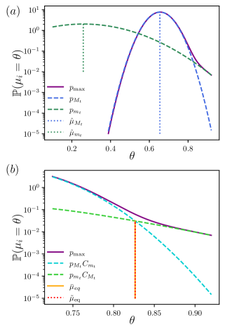
Figure 1: (a) Posterior distributions of a two-armed bandit with Gaussian rewards. The dotted lines represent the individual posterior distributions of each arm while the continuous line represents the posterior of the maximum mean reward of all arms (Eq. 4). (b) Zoom of (a) in the region where both arms have the same posterior probability of being the best one. $p_{M_{t}}C_{m_{t}}$ ($p_{m_{t}}C_{M_{t}}$) is the probability that the maximal value is given by the better (worse) empirical arm.

For Gaussian reward distributions, one can first derive an analytic expression for $\tilde{\mu}_{\mathrm{eq}}$ (see Section A.2 for details):

$$\begin{split}&\tilde{\mu}_{\mathrm{eq}}=\hat{\mu}_{M_{t}}+\frac{N_{m_{t}}(\hat{\mu}_{M_{t}}-\hat{\mu}_{m_{t}})}{N_{M_{t}}-N_{m_{t}}}+..\\ &\hskip 8.5359pt\sqrt{\frac{N_{M_{t}}N_{m_{t}}(\hat{\mu}_{M_{t}}-\hat{\mu}_{m_{t}})^{2}}{(N_{M_{t}}-N_{m_{t}})^{2}}+\frac{\sigma^{2}}{N_{M_{t}}-N_{m_{t}}}\ln\left(\frac{N_{M_{t}}}{N_{m_{t}}}\right)}.\end{split}$$ (9)

Hence, for Gaussian reward distributions Eq. 7 can be rewritten as (see Section A.4):

$$\begin{split}\tilde{S}_{\mathrm{tail}}&=\frac{1}{4}\ln(\frac{2\pi\sigma^{2}e}{N_{m_{t}}})\mathrm{erfc}\left(\frac{\sqrt{N_{m_{t}}}(\tilde{\mu}_{\mathrm{eq}}-\hat{\mu}_{m_{t}})}{\sqrt{2\sigma^{2}}}\right)\\ &\hskip 28.45274pt+\frac{\sqrt{N_{m_{t}}}(\tilde{\mu}_{\mathrm{eq}}-\hat{\mu}_{m_{t}})}{2\sqrt{2\pi\sigma^{2}}}e^{-\frac{-N_{m_{t}}(\tilde{\mu}_{\mathrm{eq}}-\hat{\mu}_{m_{t}})^{2}}{2\sigma^{2}}}.\\ \end{split}$$ (10)

Similarly for $\tilde{S}_{\mathrm{body}}$, we obtain for Gaussian rewards (see Section A.3):

$$\begin{split}\tilde{S}_{\mathrm{body}}&=\frac{1}{2}\ln\left(\frac{2\pi\sigma^{2}e}{N_{M_{t}}}\right)\times..\\ &\left[1-\frac{1}{2}\mathrm{erfc}\left(\frac{\sqrt{N_{m_{t}}N_{M_{t}}}(\hat{\mu}_{M_{t}}-\hat{\mu}_{m_{t}})}{\sqrt{2\sigma^{2}(N_{m_{t}}+N_{M_{t}})}}\right)\right]\\ &-\frac{\sqrt{N_{M_{t}}}N_{m_{t}}^{3/2}(\hat{\mu}_{M_{t}}-\hat{\mu}_{m_{t}})}{2\sigma\sqrt{2\pi}(N_{M_{t}}+N_{m_{t}})^{3/2}}e^{-\frac{N_{m_{t}}N_{M_{t}}(\hat{\mu}_{M_{t}}-\hat{\mu}_{m_{t}})^{2}}{2\sigma^{2}(N_{m_{t}}+N_{M_{t}})}}.\\ \end{split}$$ (11)

At this stage, even if we have already obtained a closed-form expression for $S_{\mathrm{\max}}$, it remains too involved to directly compute its exact (discrete) gradient for our decision policy. To finally derive a simplified gradient, we opt to retain asymptotic expressions of Eq. 10 and Eq. 11 and of the obtained gradient (see Section A.5 for derivation details). Finally, the expression of our approximate difference of gradients of the entropy functional reads:

$$\begin{split}\Delta&=\frac{1}{2}\ln(\frac{N_{m_{t}}}{N_{m_{t}}+1})+\frac{1}{4N_{M_{t}}}\mathrm{erfc}\left(\frac{\sqrt{N_{m_{t}}}(\tilde{\mu}_{\mathrm{eq}}-\hat{\mu}_{m_{t}})}{\sqrt{2\sigma^{2}}}\right)\\ &\hskip 14.22636pt+\frac{\sqrt{N_{m_{t}}}(\tilde{\mu}_{\mathrm{eq}}-\hat{\mu}_{m_{t}})}{\sqrt{2\pi\sigma^{2}}}e^{-\frac{N_{m_{t}}(\tilde{\mu}_{\mathrm{eq}}-\hat{\mu}_{m_{t}})^{2}}{2\sigma^{2}}}\times\\ &\hskip 14.22636pt\bigg{[}\frac{2N_{M_{t}}^{2}-3N_{m_{t}}^{2}}{4N_{m_{t}}N_{M_{t}}^{2}}+\frac{1}{4}\ln\left(\frac{N_{M_{t}}}{2\pi\sigma^{2}e}\right)\frac{N_{m_{t}}^{3}+N_{M_{t}}^{2}}{N_{m_{t}}^{2}N_{M_{t}}^{2}}\\ &\hskip 91.04872pt+\frac{(N_{m_{t}}^{3}+N_{M_{t}}^{2})(\tilde{\mu}_{\mathrm{eq}}-\hat{\mu}_{m_{t}})^{2}}{4\sigma^{2}N_{m_{t}}N_{M_{t}}^{2}}\bigg{]}.\\ \end{split}$$ (12)

In words, $\Delta$ approximates the difference

$$\begin{split}\Delta\approx&\phantom{-}\mathbb{E}\left[S_{\mathrm{\max}}(t)\mid\mathcal{F}_{t-1},a_{t}=M_{t}\right]\\ &-\mathbb{E}\left[S_{\mathrm{\max}}(t)\mid\mathcal{F}_{t-1},a_{t}=m_{t}\right],\end{split}$$

which is directly related to the greedy choice maximizing the entropy decrease, described in Eq. 5.

The decision procedure can be summarized as follows: if Eq. 12 is negative, the better empirical arm is chosen as it reduces the most our entropy approximation in expectation. Inversely, if Eq. 12 is positive, the worse empirical arm is chosen.

In conclusion, we have derived an analytical expression obtained from the information measure of the maximum posterior. Furthermore, it allows us to isolate an analytically tractable gradient acting as a decision procedure that eluded previous approximated information derivations. We now provide the full AIM implementation and bound its regret in the next section.

3.3 Approximate information maximization algorithm

The pseudo-code of AIM algorithm is presented in Algorithm 1 below.

Draw each arm once; observe reward $X_{t}(t)$ and update statistics $\hat{\mu}_{t}\leftarrow X_{t}(t),N_{t}\leftarrow 1\,\,\forall t\in\{1,2\}$

for $t=3$ to $T$ do

       /* Arm selection */

       $M_{t}\leftarrow\operatorname*{\arg\!\max}_{k=1,2}\hat{\mu}_{k}$, $m_{t}\leftarrow\operatorname*{\arg\!\min}_{k=1,2}\hat{\mu}_{k}$;

       if $N_{M_{t}}\leq N_{m_{t}}$ then

            $a_{t}\leftarrow M_{t}$

      else

             Evaluate $\Delta$ following Eq. 12 ;

            

            if $\Delta<0$ then

                  $a_{t}\leftarrow M_{t}$

            else

                  $a_{t}\leftarrow m_{t}$

            

      Pull $a_{t}$ and observe $X_{t}(a_{t})$

      /* Update statistics */

       $\hat{\mu}_{a_{t}}\leftarrow\frac{\hat{\mu}_{a_{t}}N_{a_{t}}+X_{t}(a_{t})}{N_{a_{t}}+1}$, $N_{a_{t}}\leftarrow N_{a_{t}}+1$

Algorithm 1 AIM Algorithm for $2$ Gaussian arm

The better empirical arm is drawn by default if ${N_{M_{t}}\leq N_{m_{t}}}$. In such a case, both entropy components in Eq. 6 are mainly contributed to by $M_{t}$ since the better empirical arm has been less selected than the worse empirical one.

4 Regret bound

This section provides theoretical guarantees on the performance of AIM.  More precisely, Theorem 1 below states that AIM is asymptotically optimal on the two-armed bandits problem with Gaussian rewards.

Theorem 1.

For Gaussian reward distributions with unit variance, the regret of AIM satisfies for any mean vector $(\mu_{1},\mu_{2})$

$$\limsup_{T\to\infty}\frac{{R}(T)}{\ln(T)}\leq\frac{2\sigma^{2}\ln(T)}{|\mu_{1}-\mu_{2}|}.$$

With Gaussian rewards, the asymptotic regret of AIM thus exactly reaches the lower bound of Lai et al. (1985) given by Eq. 2. A non-asymptotic version of Theorem 1 is given by Theorem 2 in Appendix B. We briefly sketch the proof idea below, and the complete proof is deferred to Appendix B.

Sketch of the proof.

We assume without loss of generality here and in the proof that $\mu_{1}>\mu_{2}$. Although very different in the demonstration, the structure of the proof is borrowed from Kaufmann et al. (2012a). In particular, the first main step is showing that the optimal arm is pulled at least a polynomial (in $t$) number of times with high probability. This result holds because otherwise, the contribution of the arm $1$ in the tail of the information entropy would dominate the contribution of the arm $2$ in the approximate information. In that case, pulling the first arm would naturally lead to a larger decrease in entropy, which ensures that the optimal arm is always pulled a significant amount of times.

From there, we only need to work in the asymptotic regime where both arms $1$ and $2$ are pulled a lot of times. We can ignore low-probability events and restrict the analysis to cases where empirical means of the arms do not significantly deviate from the true means. An important property of the entropy is that it approximates the behaviour of the bound of Lai et al. (1985). More precisely, in the asymptotic regime, the difference $\Delta$ of the entropy gradients almost behaves as

$$\Delta\approx-\frac{1}{2N_{M_{t}}}+\mathrm{poly}(N_{m_{t}})e^{-\frac{N_{m_{t}}(\mu_{1}-\mu_{2})^{2}}{2\sigma^{2}}},$$ (13)

where $\mathrm{poly}(N_{m_{t}})$ is some positive polynomial in $N_{m_{t}}$. In the asymptotic regime, we thus naturally have $N_{m_{t}}$ of order $\frac{2\sigma^{2}\ln T}{(\mu_{1}-\mu_{2})^{2}}$. ∎

Moreover, the required form of the entropy for the proof is very general. As long as we are guaranteed that the optimal arm will be pulled a significant amount of times with high probability and that the asymptotic regime behaves as Eq. 13, the algorithm yields an optimal regret. Hence, Theorem 1 should hold for a large family of entropy approximations (and likely for free energy generalization too, as in Masson, 2013), as long as the approximation is accurate enough to not yield trivial behaviors in the short time regime. Additionally, the approximate framework we devised here allows tuned formulas, in which individual terms ensure asymptotic optimality and the coefficients in front of them can be adjusted to improve short-time performance.

5 Experiments

This section investigates the empirical performance of AIM (Algorithm 1) on numerical examples. All details of the numerical experiments are given in Appendix D.

We start by considering two arms, with Gaussian rewards (Honda and Takemura, 2010) of unit variance and means $\mu_{k}$ drawn uniformly in $[0,1]$. Fig. 2 compares the Bayesian regret (i.e., the regret averaged over all values of $(\mu_{1},\mu_{2})$ in $[0,1]\times[0,1]$) of Algorithm 1 with the state-of-the-art algorithms UCB-tuned and Thompson sampling (Kaufmann et al., 2012b; Pilarski et al., 2021; Cappé et al., 2013) (see Section D.4 for detailed descriptions of the algorithms and an overview of other classic bandit strategies). The Bayesian regret of AIM empirically scales as $\log\left(t\right)$. Its long-time performance matches Thompson sampling, as implied by Theorem 1, while relying on a (conditionally) deterministic decision process. Additionally, AIM outperforms Thompson sampling at both short and intermediate times. AIM particularly outperforms Thompson sampling in instances where the arms are difficult to distinguish due to their mean rewards being close (see examples in Section D.5.1).

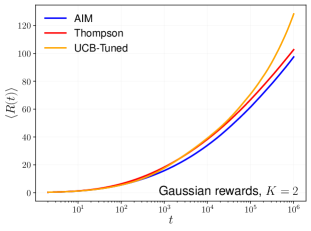
Figure 2: Evolution of the Bayesian regret for 2-armed bandit with Gaussian rewards under a uniform mean prior. The regret is averaged over more than $10^{5}$ runs.

AIM yields strong performance in the two-armed Gaussian rewards case, as predicted by our theoretical analysis. We now aim at extending our method to other bandit settings. Figs. 3 and 4 present the performance of AIM when adapted to Bernoulli reward distributions and bandits with more than two arms. These adaptations are described in detail in Section 6 below.

Fig. 3 considers Bernoulli distributed rewards (Pilarski et al., 2021) with arm means drawn uniformly in $[0,1]$. The performance of AIM is comparable to Thompson sampling here. Additionally, AIM shows comparable performance to Thompson sampling for close mean rewards (see Section D.5.2).

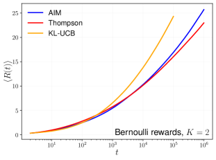
Figure 3: Evolution of the Bayesian regret for 2-armed bandit with Bernoulli rewards under a uniform mean prior. The regret is averaged over more than $10^{5}$ runs.

Fig. 4 investigates AIM,  for $50$ arms with Bernoulli rewards and means drawn uniformly in $[0,1]$. Its short-time efficiency is comparable to Thompson sampling and it is significantly more efficient at intermediary times, while showing the same logarithmic scaling at long time as Thompson sampling.

These observations support the robustness of AIM and its potential for extensions to more complex bandit settings.

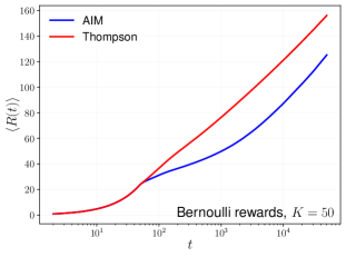
Figure 4: Evolution of the Bayesian regret for 50-armed bandit with Bernoulli rewards under a uniform mean prior. The regret is averaged over $4\times 10^{4}$ runs.

6 Extensions

We have applied our approach (above) to Bernouilli bandits with many arms, where it shows strong empirical performances (see Figs. 3 and 4). This section describes the extensions of AIM to these cases and discusses potential extensions to more general bandit settings.

Exponential family bandits.

Since Eq. 4 explicitly relies on arm posterior distributions, information maximization methods can be directly extended to various reward distributions. In particular, when the reward distributions belong to the exponential family (see Korda et al., 2013, and Section C.1 for details on such distributions), an asymptotic and analytic expression of the entropy can be derived for the case of uniform priors (see Appendix C for more details), yielding

$$\begin{split}\tilde{S}_{\mathrm{max}}&=\frac{1}{2}\ln(2\pi\bar{\sigma}^{2}_{i})\left[1-\frac{e^{-N_{m_{t}}\mathrm{KL}(\hat{\mu}_{m_{t}},\tilde{\mu}_{\mathrm{eq}})}}{N_{m_{t}}\partial_{2}\mathrm{KL}(\hat{\mu}_{m_{t}},\tilde{\mu}_{\mathrm{eq}})\sqrt{2\pi\bar{\sigma}^{2}_{m_{t}}}}\right]\\ &\hskip 62.59596pt+\frac{\mathrm{KL}(\hat{\mu}_{m_{t}},\tilde{\mu}_{\mathrm{eq}})e^{-N_{m_{t}}\mathrm{KL}(\hat{\mu}_{m_{t}},\tilde{\mu}_{\mathrm{eq}})}}{\partial_{2}\mathrm{KL}(\hat{\mu}_{m_{t}},\tilde{\mu}_{\mathrm{eq}})\sqrt{2\pi\bar{\sigma}^{2}_{m_{t}}}}.\end{split}$$ (14)

Here $\mathrm{KL}(\hat{\mu}_{i},\tilde{\mu}_{\mathrm{eq}})$ is the Kullback-Leibler divergence between the reward distributions, parameterized by $\hat{\mu}_{i}$ and $\tilde{\mu}_{\mathrm{eq}}$, respectively, and $\partial_{2}\mathrm{KL}$ denotes its derivative w.r.t. the second variable. All the steps leading to Eqs. 7 and 8 in Section 3 are not specific to Gaussian rewards. The main difference lies on their asymptotic simplifications obtained afterwards with Laplace’s method. Our implementation of AIM to Bernoulli rewards (a specific case of the exponential family) with Eq. 14 shows comparable performance to state-of-the-art algorithms (see Fig. 3), supporting its adaptability to general settings. We believe that AIM should be optimal for all exponential family reward distributions as well as general prior distributions (see Appendix C for a detailed discussion).

Extension to $K>2$.

The functional form of Eq. 3 offers a straightforward extension to AIM for more than two arms (Reddy et al., 2016). As for the previous settings, a similar set of simplifications have to be derived to extract an analytic expression. We will again consider the best empirical arm as the main component of the $p_{\mathrm{\max}}$ mode and approximate the worse empirical arms contributions as essentially concentrated in the tail. We thus keep a partitioning similar to Eq. 6 as

$$\tilde{S}_{\mathrm{tail}}=-\sum_{i\neq M_{t}}^{K}\int_{\tilde{\mu}_{\mathrm{eq,i}}}^{\mu_{\mathrm{sup}}}p_{i}(\theta)\ln p_{i}(\theta)\mathrm{d}\theta,$$ (15)

where $\tilde{\mu}_{\mathrm{eq,i}}$ approximates the value where arm $i$ has the same probability of being the maximum as the better empirical arm and

$$\begin{split}\tilde{S}_{\mathrm{body}}&=-\int_{\Theta}\big{(}1-\sum_{i\neq M_{t}}^{K}[1-C_{i}(\theta)]\big{)}p_{M_{t}}(\theta)\ln p_{M_{t}}(\theta)\mathrm{d}\theta.\\ \end{split}$$ (16)

Notably, Eqs. 15 and 16 summations come from the expansion at the lower order of the worse empirical arms contributions (see Section C.8 for derivation details). Hence, Eqs. 11, 10 and 14 can be directly used to get tractable expressions for any finite arms setting. An implementation for Bernoulli rewards with $K=50$ is displayed Fig. 4, where AIM shows comparable performances to Thompson Sampling on large times and strongly outperform Thompson sampling on short time scales. Finally, since Eqs. 15 and 16 resemble the expression in the case of two arms, we believe that AIM should also be optimal for $K>2$ arms and that similar proof techniques can be used.

Other bandits settings.

At last, we provide a quick overview of several more complex bandit settings for which the information maximization should build to the specific bandit structure of the problem to provide efficient algorithms. First, we emphasize that AIM partition between body/tail components remains relevant even when dealing with heavy-tailed (Lee et al., 2023) or non-parametric reward distributions (Baudry et al., 2020); it should thus be able to provide strong guarantees in these settings, similarly to Thompson sampling. Secondly, let us stress that information can also be quantified for unpulled arms, which may prove crucial when facing a large number of arms. The agent could quantify the information of the “reservoir” of unpulled arms, to anticipate the information gain of exploring these unpulled arms. Additionally, if the agent has access to the remaining time, it can not only evaluate the expected information gain when pulling an arm for a single round, but instead evaluate the information gain of multiple pulls of the same arm. We believe that such a consideration might be pivotal when facing many arms, since the limited amount of time does not allow to pull all the arms (Bayati et al., 2020) sufficiently. Thirdly, one can consider linear bandits, where arms are correlated with each other (Li et al., 2010). Because pulling a specific direction directly provides side information on correlated directions, the shared information gain could be leveraged by information-based methods to yield strong performances. Finally, one could consider pure exploration problems (Bubeck et al., 2011; Locatelli et al., 2016; Kalyanakrishnan et al., 2012) where the agent’s goal is directly linked to an information gain, thus making the information maximization principle an inherent candidate when a suitable entropy is derived from the underlying bandit structure and problem objective. A last advantage of AIM lies in its possible extension to multiple constraints that would be introduced using Lagrange multipliers (or borrowed from physics reasoning by defining a free energy), further improving its adaptability to various settings and to specific requirements.

7 Conclusion

This paper introduces a new algorithm class, AIM, which leverages approximate information maximization of the whole bandit system to achieve optimal regret performances. This approach builds on the entropy of the posterior of the arms’ maximal mean, from which we extract a simplified and analytical functional at the core of the decision schemes. It enables easily tunable and tractable algorithms, which we prove to be optimal in for two-armed Gaussian bandits. Numerical experiments for Bernoulli rewards with two or several arms emphasise robustness and efficiency of AIM. An additional strength of AIM lies in its efficiency at short times and when the arms have close mean rewards. Further research should focus on adjusting the information maximization framework to more complex bandit settings, including many-armed bandits, linear bandits and thresholding bandits, where some wisely selected information measure can efficiently apprehend the arms’ structure and correlations.

Appendix A Towards an analytical approximation of the entropy

In this section, we recapitulate all the steps leading to the analytical expression constitutive of our AIM algorithm.

A.1 The partitioning approximation

We start by commenting on the partition scheme and the approximations leading to the body/tail expressions summarized below.

$$\tilde{S}_{\mathrm{tail}}=-\int_{\tilde{\mu}_{\mathrm{eq}}}^{\mu_{\mathrm{sup}}}p_{m_{t}}(\theta)\ln p_{m_{t}}(\theta)d\theta,\>\mathrm{and}\>\tilde{S}_{\mathrm{body}}=-\int_{\Theta}p_{M_{t}}(\theta)C_{m_{t}}(\theta)\ln p_{M_{t}}(\theta)\mathrm{d}\theta.$$ (17)

We first remind $p_{\mathrm{\max}}(\theta)$ expression with the arms order ($M_{t}$,$m_{t}$)

$$\begin{split}p_{\mathrm{\max}}(\theta)&=\left[C_{m_{t}}(\theta)p_{M_{t}}(\theta)+C_{M_{t}}(\theta)p_{m_{t}}(\theta)\right].\end{split}$$ (18)

We aim to keep the leading orders of $p_{\mathrm{\max}}(\theta)$ when $N_{M_{t}}\gg N_{m_{t}}\gg 1$ and $\hat{\mu}_{M_{t}}>\hat{\mu}_{m_{t}}$. Here, the posterior distributions are assumed uni-modal. The first term is the leading order in the vicinity of the mode of $\hat{\mu}_{M_{t}}$. Also, since $N_{M_{t}}>N_{m_{t}}$, $p_{M_{t}}(\theta)$ is more concentrated than $p_{m_{t}}(\theta)$, resulting in the dominance of the second term in the distribution tail (for the high reward side).

Thus, by defining the intersection point $\tilde{\mu}_{\mathrm{eq}}$ (where $C_{m_{t}}(\tilde{\mu}_{\mathrm{eq}})p_{M_{t}}(\tilde{\mu}_{\mathrm{eq}})=C_{M_{t}}(\tilde{\mu}_{\mathrm{eq}})p_{m_{t}}(\tilde{\mu}_{\mathrm{eq}})$), we decompose the entropy in the body/tail components defined in the main text. In the asymptotic regime, $\tilde{\mu}_{\mathrm{eq}}$ will verify $p_{m_{t}}(\theta)\gg p_{M_{t}}(\theta)$ for $\theta>\tilde{\mu}_{\mathrm{eq}}$ and $p_{m_{t}}(\theta)\ll p_{M_{t}}(\theta)$ for $\theta<\tilde{\mu}_{\mathrm{eq}}$. We neglect the transition regime where $\tilde{\mu}_{\mathrm{eq}}\sim\theta$ where both distributions are of the same order because it is narrow (in the asymptotic regime) and have a very little influence on the total value of the entropy.

We now consider the tail where $\theta>\tilde{\mu}_{\mathrm{eq}}$ implying $p_{m_{t}}(\theta)\gg p_{M_{t}}(\theta)$. Because $N_{m_{t}}\gg 1$, we get $C_{m_{t}}(\theta)\approx 1$. Noticing that $C_{M_{t}}(\theta)>C_{m_{t}}(\theta)$, we also get $C_{M_{t}}(\theta)\approx 1$. Applying these scaling ratios, we get rid of all the subdominant terms in $\tilde{S}_{\mathrm{tail}}$:

$$\begin{split}-\tilde{S}_{\mathrm{tail}}&\sim\int_{\tilde{\mu}_{\mathrm{eq}}}^{\mu_{\mathrm{sup}}}\left[C_{m_{t}}(\theta)p_{M_{t}}(\theta)+C_{M_{t}}(\theta)p_{m_{t}}(\theta)\right]\log\left[C_{m_{t}}(\theta)p_{M_{t}}(\theta)+C_{M_{t}}(\theta)p_{m_{t}}(\theta)\right]\mathrm{d}\theta\\ &\sim\int_{\tilde{\mu}_{\mathrm{eq}}}^{\mu_{\mathrm{sup}}}C_{M_{t}}(\theta)p_{m_{t}}(\theta)\log\left[C_{M_{t}}(\theta)p_{m_{t}}(\theta)\right]+C_{m_{t}}(\theta)p_{M_{t}}(\theta)+o(C_{m_{t}}(\theta)p_{M_{t}}(\theta))\mathrm{d}\theta\\ &\hskip 56.9055pt+\int_{\tilde{\mu}_{\mathrm{eq}}}^{\mu_{\mathrm{sup}}}C_{m_{t}}(\theta)p_{M_{t}}(\theta)\log\left[C_{m_{t}}(\theta)p_{M_{t}}(\theta)+C_{M_{t}}(\theta)p_{m_{t}}(\theta)\right]\mathrm{d}\theta\\ &\sim\int_{\tilde{\mu}_{\mathrm{eq}}}^{\mu_{\mathrm{sup}}}p_{m_{t}}(\theta)\log\left[p_{m_{t}}(\theta)\right][1+\mathcal{O}\left(1-C_{M_{t}}(\tilde{\mu}_{\mathrm{eq}})\right)]+\mathcal{O}\left(p_{M_{t}}(\theta)\log[p_{m_{t}}(\theta)]\right)\mathrm{d}\theta,\\ &\sim\int_{\tilde{\mu}_{\mathrm{eq}}}^{\mu_{\mathrm{sup}}}p_{m_{t}}(\theta)\log\left[p_{m_{t}}(\theta)\right]\mathrm{d}\theta\\ \end{split}$$ (19)

where we used that $C_{M_{t}}(\theta)=1-\int_{\theta}^{\mu_{\mathrm{sup}}}p_{M_{t}}(\theta)d\theta<C_{M_{t}}(\tilde{\mu}_{\mathrm{eq}})$.

We finally consider the body term. Noticing that $p_{M_{t}}(\theta)\gg p_{m_{t}}(\theta)$, $\tilde{S}_{\mathrm{body}}$ reads

$$\begin{split}-\tilde{S}_{\mathrm{body}}&\sim\int_{\mu_{\mathrm{inf}}}^{\tilde{\mu}_{\mathrm{eq}}}\left[C_{m_{t}}(\theta)p_{M_{t}}(\theta)+C_{M_{t}}(\theta)p_{m_{t}}(\theta)\right]\log\left[C_{m_{t}}(\theta)p_{M_{t}}(\theta)+C_{M_{t}}(\theta)p_{m_{t}}(\theta)\right]\mathrm{d}\theta\\ &\sim\int_{\mu_{\mathrm{inf}}}^{\tilde{\mu}_{\mathrm{eq}}}C_{m_{t}}(\theta)p_{M_{t}}(\theta)\log\left[C_{m_{t}}(\theta)p_{M_{t}}(\theta)\right]+C_{M_{t}}(\theta)p_{m_{t}}(\theta)+o(C_{M_{t}}(\theta)p_{m_{t}}(\theta))d\theta\\ &\hskip 56.9055pt+\int_{\mu_{\mathrm{inf}}}^{\tilde{\mu}_{\mathrm{eq}}}C_{M_{t}}(\theta)p_{m_{t}}(\theta)\log\left[C_{m_{t}}(\theta)p_{M_{t}}(\theta)+C_{M_{t}}(\theta)p_{m_{t}}(\theta)\right]\mathrm{d}\theta\\ &\sim\int_{\mu_{\mathrm{inf}}}^{\tilde{\mu}_{\mathrm{eq}}}C_{m_{t}}(\theta)p_{M_{t}}(\theta)\log\left[p_{M_{t}}(\theta)\right][1+o(1)]+o(p_{M_{t}}(\theta))\mathrm{d}\theta,\\ \end{split}$$ (20)

where we have used that $p_{M_{t}}(\theta)\gg 1$ around the vicinity of $\hat{\mu}_{M_{t}}$. Since, the inner term of the integral is negligible for $\theta>\tilde{\mu}_{\mathrm{eq}}$ (by definition of $\tilde{\mu}_{\mathrm{eq}}$), we extend the upper bound of Eq. 20 to the full integration domain without loss of consistency. It will simplify the derivation of an analytical expression for the body component in the next section. Taking altogether the leading orders of Eqs. 19 and 20 gives Eq. 17.

A.2 Asymptotic of the intersection point

In this section we derive the asymptotic expression of the intersection point (defined above as $\tilde{\mu}_{\mathrm{eq}}$) where the distributions $C_{m_{t}}(\tilde{\mu}_{\mathrm{eq}})p_{M_{t}}(\tilde{\mu}_{\mathrm{eq}})$ and $C_{M_{t}}(\tilde{\mu}_{\mathrm{eq}})p_{m_{t}}(\tilde{\mu}_{\mathrm{eq}})$ intersect at their highest value (if they intersect more than once). Here we consider Gaussian rewards. The exact equation verified by the intersection point $\bar{\mu}_{\mathrm{eq}}$ is

$$\begin{split}&\frac{\sqrt{N_{M_{t}}}e^{-\frac{N_{M_{t}}(\bar{\mu}_{\mathrm{eq}}-\hat{\mu}_{M_{t}})^{2}}{2\sigma^{2}}}}{\sqrt{2\pi\sigma^{2}}}\frac{1}{2}\left[1+\mathrm{erf}\left(\frac{\sqrt{N_{m_{t}}}(\bar{\mu}_{\mathrm{eq}}-\hat{\mu}_{m_{t}})}{\sqrt{2\sigma^{2}}}\right)\right]=\frac{\sqrt{N_{m_{t}}}e^{-\frac{N_{m_{t}}(\bar{\mu}_{\mathrm{eq}}-\hat{\mu}_{m_{t}})^{2}}{2\sigma^{2}}}}{\sqrt{2\pi\sigma^{2}}}\frac{1}{2}\left[1+\mathrm{erf}\left(\frac{\sqrt{N_{M_{t}}}(\bar{\mu}_{\mathrm{eq}}-\hat{\mu}_{M_{t}})}{\sqrt{2\sigma^{2}}}\right)\right].\\ \end{split}$$ (21)

Taking the logarithm of Eq. 21 and normalizing the last term leads to

$$\begin{split}&\frac{N_{m_{t}}(\bar{\mu}_{\mathrm{eq}}-\hat{\mu}_{m_{t}})^{2}}{2\sigma^{2}}-\frac{N_{M_{t}}(\bar{\mu}_{\mathrm{eq}}-\hat{\mu}_{M_{t}})^{2}}{2\sigma^{2}}+\frac{1}{2}\ln\frac{N_{M_{t}}}{N_{m_{t}}}+\ln\left[\frac{1+\mathrm{erf}\left(\frac{\sqrt{N_{m_{t}}}(\bar{\mu}_{\mathrm{eq}}-\hat{\mu}_{m_{t}})}{\sqrt{2\sigma^{2}}}\right)}{1+\mathrm{erf}\left(\frac{\sqrt{N_{M_{t}}}(\bar{\mu}_{\mathrm{eq}}-\hat{\mu}_{M_{t}})}{\sqrt{2\sigma^{2}}}\right)}\right]=0.\end{split}$$ (22)

The distributions are uni-modal, and assuming that $\hat{\mu}_{M_{t}}>\hat{\mu}_{m_{t}}$, $N_{M_{t}}>N_{m_{t}}$ and recalling that $\bar{\mu}_{\mathrm{eq}}$ is the highest intersection solution, we get that $\bar{\mu}_{\mathrm{eq}}>\hat{\mu}_{M_{t}}>\hat{\mu}_{m_{t}}$. Both error functions are then bounded in $[0,1]$ making the last term also bounded. We then approximate $\bar{\mu}_{\mathrm{eq}}$ with $\tilde{\mu}_{\mathrm{eq}}$ by neglecting the last term which leads to the following solution:

$$\begin{split}&\tilde{\mu}_{\mathrm{eq}}=\hat{\mu}_{M_{t}}+\frac{N_{m_{t}}(\hat{\mu}_{M_{t}}-\hat{\mu}_{m_{t}})}{N_{M_{t}}-N_{m_{t}}}+\sqrt{\frac{N_{M_{t}}N_{m_{t}}}{(N_{M_{t}}-N_{m_{t}})^{2}}(\hat{\mu}_{M_{t}}-\hat{\mu}_{m_{t}})^{2}+\frac{\sigma^{2}}{N_{M_{t}}-N_{m_{t}}}\ln\left(\frac{N_{M_{t}}}{N_{m_{t}}}\right)}.\end{split}$$ (23)

Note that Eq. 23 expression relies on both $\hat{\mu}_{M_{t}}>\hat{\mu}_{m_{t}}$ and $N_{M_{t}}>N_{m_{t}}$. For $N_{M_{t}}\leq N_{m_{t}}$, even if the above $\tilde{\mu}_{\mathrm{eq}}$ can be computed, it doesn’t quantify the tail contribution. As a matter of fact, for $N_{M_{t}}\leq N_{m_{t}}$, the tail is always dominated by $p_{M_{t}}$ which means that it has been already included in the main mode $\tilde{S}_{\mathrm{body}}$. Then, in this specific configuration, we take $\tilde{S}_{\mathrm{tail}}$ equals to $0$ and $\tilde{\mu}_{\mathrm{eq}}=\mu_{\mathrm{sup}}$.

A.3 Closed-form expressions for the main mode’s contribution

Here, we derive the $\tilde{S}_{\mathrm{body}}$ expression given in the main text for Gaussian rewards distribution. Inserting the Gaussian form of the posterior into Eq. 8 gives:

$$\begin{split}\tilde{S}_{\mathrm{body}}=&-\int_{-\infty}^{+\infty}\frac{\sqrt{N_{M_{t}}}e^{-\frac{N_{M_{t}}(\theta-\hat{\mu}_{M_{t}})^{2}}{2\sigma^{2}}}}{\sqrt{2\pi\sigma^{2}}}\frac{1}{2}\left[1+\mathrm{erf}\left(\frac{\sqrt{N_{m_{t}}}(\theta-\hat{\mu}_{m_{t}})}{\sqrt{2\sigma^{2}}}\right)\right]\left(-\frac{1}{2}\ln(\frac{2\pi\sigma^{2}}{N_{M_{t}}})-\frac{N_{M_{t}}(\theta-\hat{\mu}_{M_{t}})^{2}}{2\sigma^{2}}\right)\mathrm{d}\theta,\end{split}$$ (24)

We integrate the constant part of the first term by use of the following identity (Ng and Geller, 1969):

$$\begin{split}\int_{-\infty}^{\infty}&\bigg{[}1+\mathrm{erf}\left(\frac{\theta-\theta_{1}}{\sqrt{2V_{1}}}\right)\bigg{]}\frac{e^{-\frac{(\theta-\theta_{2})^{2}}{2V_{2}}}}{\sqrt{2\pi V_{2}}}\mathrm{d}\theta=\left[1+\mathrm{erf}\left(\frac{\theta_{2}-\theta_{1}}{\sqrt{2}\sqrt{V_{2}+V_{1}}}\right)\right],\end{split}$$ (25)

which leads to

$$\begin{split}&\int_{-\infty}^{+\infty}\frac{\sqrt{N_{M_{t}}}e^{-\frac{N_{M_{t}}(\theta-\hat{\mu}_{M_{t}})^{2}}{2\sigma^{2}}}}{\sqrt{2\pi\sigma^{2}}}\left[1+\mathrm{erf}\left(\frac{\sqrt{N_{m_{t}}}(\theta-\hat{\mu}_{m_{t}})}{\sqrt{2\sigma^{2}}}\right)\right]\mathrm{d}\theta=\left[1+\mathrm{erf}\left(\frac{\hat{\mu}_{M_{t}}-\hat{\mu}_{m_{t}}}{\sqrt{2\sigma^{2}(\frac{1}{N_{M_{t}}}+\frac{1}{N_{m_{t}}})}}\right)\right].\end{split}$$ (26)

Next, we integrate by parts the second term to obtain:

$$\begin{split}&\int_{-\infty}^{\infty}\frac{N_{M_{t}}(\theta-\hat{\mu}_{M_{t}})^{2}}{2\sigma^{2}}\frac{\sqrt{N_{M_{t}}}e^{-\frac{N_{M_{t}}(\theta-\hat{\mu}_{M_{t}})^{2}}{2\sigma^{2}}}}{\sqrt{2\pi\sigma^{2}}}\frac{1}{2}\left[1+\mathrm{erf}\left(\frac{\sqrt{N_{m_{t}}}(\theta-\hat{\mu}_{m_{t}})}{\sqrt{2\sigma^{2}}}\right)\right]\mathrm{d}\theta\\ &=\int_{-\infty}^{\infty}\frac{1}{4}\frac{\sqrt{N_{M_{t}}}e^{-\frac{N_{M_{t}}(\theta-\hat{\mu}_{M_{t}})^{2}}{2\sigma^{2}}}}{\sqrt{2\pi\sigma^{2}}}\left[1+\mathrm{erf}\left(\frac{\sqrt{N_{m_{t}}}(\theta-\hat{\mu}_{m_{t}})}{\sqrt{2\sigma^{2}}}\right)\right]+\frac{(\theta-\hat{\mu}_{M_{t}})}{2}\frac{\sqrt{N_{M_{t}}N_{m_{t}}}e^{-\frac{N_{M_{t}}(\theta-\hat{\mu}_{M_{t}})^{2}}{2\sigma^{2}}-\frac{N_{m_{t}}(\theta-\hat{\mu}_{m_{t}})^{2}}{2\sigma^{2}}}}{2\pi\sigma^{2}}\mathrm{d}\theta\\ &=\frac{1}{4}\left[1+\mathrm{erf}\left(\frac{\hat{\mu}_{M_{t}}-\hat{\mu}_{m_{t}}}{\sqrt{2\sigma^{2}(\frac{1}{N_{M_{t}}}+\frac{1}{N_{m_{t}}})}}\right)\right]+\frac{(\hat{\mu}_{m_{t}}-\hat{\mu}_{M_{t}})\sigma^{2}}{2N_{M_{t}}\sqrt{2\pi}(\frac{\sigma^{2}}{N_{M_{t}}}+\frac{\sigma^{2}}{N_{m_{t}}})^{3/2}}e^{-\frac{ (\hat{\mu}_{M_{t}}-\hat{\mu}_{m_{t}})^{2}}{2\sigma^{2}(\frac{1}{N_{M_{t}}}+\frac{1}{N_{m_{t}}})}},\end{split}$$ (27)

where we also rely on the identity of Eq. 25.

Combining Eqs. 26 and 27 leads to the analytical expression of the body component.

$$\begin{split}\tilde{S}_{\mathrm{body}}&=\frac{1}{2}\ln(\frac{2\pi\sigma^{2}e}{N_{M_{t}}})\left[1-\frac{1}{2}\mathrm{erfc}\left(\frac{\sqrt{N_{m_{t}}N_{M_{t}}}(\hat{\mu}_{M_{t}}-\hat{\mu}_{m_{t}})}{\sqrt{2\sigma^{2}(N_{m_{t}}+N_{M_{t}})}}\right)\right]-\frac{\sqrt{N_{M_{t}}}N_{m_{t}}^{3/2}(\hat{\mu}_{M_{t}}-\hat{\mu}_{m_{t}})}{2\sigma\sqrt{2\pi}(N_{M_{t}}+N_{m_{t}})^{3/2}}e^{-\frac{N_{m_{t}}N_{M_{t}}(\hat{\mu}_{M_{t}}-\hat{\mu}_{m_{t}})^{2}}{2\sigma^{2}(N_{m_{t}}+N_{M_{t}})}}.\\ \end{split}$$ (28)

To finally get an asymptotic and simplified expression of the body component, we neglect the second term. Then, since $\tilde{\mu}_{\mathrm{eq}}\underset{N_{M_{t}}\to\infty}{\longrightarrow}\hat{\mu}_{M_{t}}$ and $N_{m_{t}}\ll N_{M_{t}}$ asymptotically, we approximate the first term as:

$$\begin{split}\tilde{S}_{\mathrm{b}}&=\frac{1}{2}\ln(\frac{2\pi\sigma^{2}e}{N_{M_{t}}})\left[1-\frac{1}{2}\mathrm{erfc}\left(\frac{\sqrt{N_{m_{t}}}(\tilde{\mu}_{\mathrm{eq}}-\hat{\mu}_{m_{t}})}{\sqrt{2\sigma^{2}}}\right)\right].\\ \end{split}$$ (29)

This last approximation will enable to provide an analytically tractable gradient without altering the asymptotic behavior expected at large times for the entropy measure.

A.4 Close form and asymptotic expression for the entropy tail

The contribution from the tail can be derived exactly and reads

$$\begin{split}\tilde{S}_{\mathrm{tail}}&=\int_{\tilde{\mu}_{\mathrm{eq}}}^{\infty}\frac{\sqrt{N_{m_{t}}}e^{-\frac{N_{m_{t}}(\theta-\hat{\mu}_{m_{t}})^{2}}{2\sigma^{2}}}}{\sqrt{2\pi\sigma^{2}}}\bigg{[}\frac{1}{2}\ln(\frac{2\pi\sigma^{2}}{N_{m_{t}}})+\frac{N_{m_{t}}(\theta-\hat{\mu}_{m_{t}})^{2}}{2\sigma^{2}}\bigg{]}\mathrm{d}\theta\\ &=\frac{1}{4}\ln\left(\frac{2\pi\sigma^{2}e}{N_{m_{t}}}\right)\mathrm{erfc}\left(\frac{\sqrt{N_{m_{t}}}(\tilde{\mu}_{\mathrm{eq}}-\hat{\mu}_{m_{t}})}{\sqrt{2\sigma^{2}}}\right)+\frac{\sqrt{N_{m_{t}}}(\tilde{\mu}_{\mathrm{eq}}-\hat{\mu}_{m_{t}})}{2\sqrt{2\pi\sigma^{2}}}e^{-\frac{N_{m_{t}}(\tilde{\mu}_{\mathrm{eq}}-\hat{\mu}_{m_{t}})^{2}}{2\sigma^{2}}}.\end{split}$$ (30)

To get a simplified analytical expression of the tail component, we only keep the second term since it prevails asymptotically:

$$\begin{split}\tilde{S}_{\mathrm{t}}&=\frac{\sqrt{N_{m_{t}}}(\tilde{\mu}_{\mathrm{eq}}-\hat{\mu}_{m_{t}})}{2\sqrt{2\pi\sigma^{2}}}e^{-\frac{N_{m_{t}}(\tilde{\mu}_{\mathrm{eq}}-\hat{\mu}_{m_{t}})^{2}}{2\sigma^{2}}}.\end{split}$$ (31)

Taken altogether, Eqs. 29 and 31 leads to the desired simplified approximation of the entropy:

$$\tilde{S}_{\mathrm{m}}=\tilde{S}_{\mathrm{b}}+\tilde{S}_{\mathrm{t}}.$$ (32)

A.5 Derivation of the increment for the closed-form expression of entropy.

Since, Eqs. 29 and 31 exhibit simple closed-form expressions, it becomes possible to derive an explicit expression of its expected increment. Here we again consider continuous Gaussian reward distributions.

We start by deriving the increment along the better empirical arm. The posterior of the reward obtained at time $N_{m_{t}}+N_{M_{t}}+1$ is approximated as a Gaussian of variance $\sigma^{2}$ and centred around $\hat{\mu}_{M_{t}}$, leading for the increment evaluation to:

$$\begin{split}\Delta_{M_{t}}\tilde{S}_{\mathrm{m}}&=\int_{-\infty}^{\infty}\frac{e^{-\frac{\mu^{2}}{2\sigma^{2}}}}{\sqrt{2\pi\sigma^{2}}}\bigg{[}\tilde{S}_{\mathrm{m}}(\hat{\mu}_{M_{t}}+\frac{\mu}{N_{M_{t}}+1},N_{M_{t}}+1,\hat{\mu}_{m_{t}},N_{m_{t}})-\tilde{S}_{\mathrm{m}}(\hat{\mu}_{M_{t}},N_{M_{t}},\hat{\mu}_{m_{t}},N_{m_{t}})\bigg{]}\mathrm{d}\mu.\\ \end{split}$$ (33)

For the sake of simplicity, we neglect the variations of all the subdominant terms inside $\tilde{\mu}_{\mathrm{eq}}$ meaning we approximate $\tilde{\mu}_{\mathrm{eq}}$ as $\tilde{\mu}_{\mathrm{eq}}(\hat{\mu}_{M_{t}}+\frac{\mu}{N_{M_{t}}+1},N_{M_{t}}+1,\hat{\mu}_{m_{t}},N_{m_{t}})\approx\tilde{\mu}_{\mathrm{eq}}(\hat{\mu}_{M_{t}},N_{M_{t}},\hat{\mu}_{m_{t}},N_{m_{t}})+\frac{\mu}{N_{M_{t}}+1}$, after observing a reward $\mu$ when pulling the arm $M_{t}$ for the $N_{M_{t}}\!+\!1$-th time.

By use of the identity Eq. 25, one can show that the gradient of the body component $\Delta_{M_{t}}\tilde{S}_{\mathrm{max}}$ rewrites as

$$\begin{split}\Delta_{M_{t}}\tilde{S}_{\mathrm{b}}&=\frac{1}{2}\ln(\frac{2\pi\sigma^{2}e}{N_{M_{t}}+1})\left[1-\frac{1}{2}\mathrm{erfc}\left(\frac{\sqrt{N_{m_{t}}}(\tilde{\mu}_{\mathrm{eq}}-\hat{\mu}_{m_{t}})}{\sqrt{2\sigma^{2}}\sqrt{1+\frac{N_{m_{t}}}{(N_{M_{t}}+1)^{2}}}}\right)\right]-\frac{1}{2}\ln(\frac{2\pi\sigma^{2}e}{N_{M_{t}}})\left[1-\frac{1}{2}\mathrm{erfc}\left(\frac{\sqrt{N_{m_{t}}}(\tilde{\mu}_{\mathrm{eq}}-\hat{\mu}_{m_{t}})}{\sqrt{2\sigma^{2}}}\right)\right].\\ \end{split}$$ (34)

Next, we consider the increment of the tail component along the better empirical arm:

$$\begin{split}\Delta_{M_{t}}\tilde{S}_{\mathrm{t}}&=\int_{-\infty}^{\infty}\frac{e^{-\frac{\mu^{2}}{2\sigma^{2}}}}{\sqrt{2\pi\sigma^{2}}}\frac{\sqrt{N_{m_{t}}}(\frac{\mu}{N_{M_{t}}+1}+\tilde{\mu}_{\mathrm{eq}}-\hat{\mu}_{m_{t}})}{2\sqrt{2\pi\sigma^{2}}}e^{-\frac{N_{m_{t}}(\tilde{\mu}_{\mathrm{eq}}+\frac{\mu}{N_{M_{t}}+1}-\hat{\mu}_{m_{t}})^{2}}{2\sigma^{2}}}-\tilde{S}_{\mathrm{t}}(\hat{\mu}_{M_{t}},N_{M_{t}},\hat{\mu}_{m_{t}},N_{m_{t}})\mathrm{d}\mu\\ &=e^{-N_{m_{t}}\frac{(\tilde{\mu}_{\mathrm{eq}}-\hat{\mu}_{m_{t}})^{2}}{2\sigma^{2}(1+\frac{N_{m_{t}}}{(1+N_{M_{t}})^{2}})}}\sqrt{\frac{N_{m_{t}}}{8\pi\sigma^{2}}}\frac{\left(\tilde{\mu}_{\mathrm{eq}}-\hat{\mu}_{m_{t}}\right)}{(1+\frac{N_{m_{t}}}{(N_{M_{t}}+1)^{2}})^{3/2}}-\tilde{S}_{\mathrm{t}}(\hat{\mu}_{M_{t}},N_{M_{t}},\hat{\mu}_{m_{t}},N_{m_{t}}).\\ \end{split}$$ (35)

Next, we consider the increment evaluation along the worst empirical arm.

$$\begin{split}\Delta_{m_{t}}\tilde{S}_{\mathrm{m}}&=\int_{-\infty}^{\infty}\frac{e^{-\frac{\mu^{2}}{2\sigma^{2}}}}{\sqrt{2\pi\sigma^{2}}}\bigg{[}\tilde{S}_{\mathrm{m}}(\hat{\mu}_{M_{t}},N_{M_{t}},\hat{\mu}_{m_{t}}+\frac{\mu}{N_{m_{t}}+1},N_{m_{t}}+1)-\tilde{S}_{\mathrm{m}}(\hat{\mu}_{M_{t}},N_{M_{t}},\hat{\mu}_{m_{t}},N_{m_{t}})\bigg{]}\mathrm{d}\mu.\\ \end{split}$$ (36)

We also neglect the variations of the subdominant term inside $\tilde{\mu}_{\mathrm{eq}}$. We start by considering the increment of the body component.

$$\begin{split}\Delta_{m_{t}}\tilde{S}_{\mathrm{b}}&=\frac{1}{2}\ln(\frac{2\pi\sigma^{2}e}{N_{M_{t}}})\left[1-\mathrm{erfc}\left(\frac{(N_{m_{t}}+1)(\tilde{\mu}_{\mathrm{eq}}-\hat{\mu}_{m_{t}})}{\sqrt{2\sigma^{2}(N_{m_{t}}+2)}}\right)\right]-\frac{1}{2}\ln(\frac{2\pi\sigma^{2}e}{N_{M_{t}}})\left[1-\frac{1}{2}\mathrm{erfc}\left(\frac{\sqrt{N_{m_{t}}}(\tilde{\mu}_{\mathrm{eq}}-\hat{\mu}_{m_{t}})}{\sqrt{2\sigma^{2}}}\right)\right].\\ \end{split}$$ (37)

Finally, we consider the last component of the increment along the worst empirical arm:

$$\begin{split}\Delta_{m_{t}}\tilde{S}_{\mathrm{t}}&=\int_{-\infty}^{\infty}\frac{e^{-\frac{\mu^{2}}{2\sigma^{2}}}}{\sqrt{2\pi\sigma^{2}}}\frac{\sqrt{N_{m_{t}}+1}(\frac{\mu}{N_{m_{t}}+1}+\tilde{\mu}_{\mathrm{eq}}-\hat{\mu}_{m_{t}})}{2\sqrt{2\pi\sigma^{2}}}e^{-\frac{(N_{m_{t}}+1)(\tilde{\mu}_{\mathrm{eq}}+\frac{\mu}{N_{m_{t}}+1}-\hat{\mu}_{m_{t}})^{2}}{2\sigma^{2}}}-\tilde{S}_{\mathrm{t}}(\hat{\mu}_{M_{t}},N_{M_{t}},\hat{\mu}_{m_{t}},N_{m_{t}})\mathrm{d}\mu\\ &=e^{-\frac{(N_{m_{t}}+1)^{2}}{(N_{m_{t}}+2)}\frac{(\tilde{\mu}_{\mathrm{eq}}-\hat{\mu}_{m_{t}})^{2}}{2\sigma^{2}}}\frac{(1+N_{m_{t}})^{2}\left(\tilde{\mu}_{\mathrm{eq}}-\hat{\mu}_{m_{t}}\right)}{\sqrt{8\pi\sigma^{2}}(2+N_{m_{t}})^{3/2}}.-\tilde{S}_{\mathrm{t}}(\hat{\mu}_{M_{t}},N_{M_{t}},\hat{\mu}_{m_{t}},N_{m_{t}})\\ \end{split}$$ (38)

Taken altogether, Eqs. 34, 35, 37 and 38 leads to the final analytical expression of the increment:

$$\begin{split}\Delta_{M_{t}}\tilde{S}_{\mathrm{m}}-\Delta_{m_{t}}\tilde{S}_{\mathrm{m}}&=\frac{1}{2}\ln(\frac{2\pi\sigma^{2}e}{N_{M_{t}}+1})\left[1-\frac{1}{2}\mathrm{erfc}\left(\frac{\sqrt{N_{m_{t}}}(\tilde{\mu}_{\mathrm{eq}}-\hat{\mu}_{m_{t}})}{\sqrt{2\sigma^{2}}\sqrt{1+\frac{N_{m_{t}}}{(N_{M_{t}}+1)^{2}}}}\right)\right]\\ &\hskip 2.84544pt-\frac{1}{2}\ln(\frac{2\pi\sigma^{2}e}{N_{M_{t}}})\left[1-\frac{1}{2}\mathrm{erfc}\left(\frac{(N_{m_{t}}+1)(\tilde{\mu}_{\mathrm{eq}}-\hat{\mu}_{m_{t}})}{\sqrt{2\sigma^{2}(N_{m_{t}}+2)}}\right)\right]\\ &\hskip 2.84544pt+e^{-N_{m_{t}}\frac{(\tilde{\mu}_{\mathrm{eq}}-\hat{\mu}_{m_{t}})^{2}}{2\sigma^{2}(1+\frac{N_{m_{t}}}{(1+N_{M_{t}})^{2}})}}\sqrt{\frac{N_{m_{t}}}{8\pi\sigma^{2}}}\frac{\left(\tilde{\mu}_{\mathrm{eq}}-\hat{\mu}_{m_{t}}\right)}{(1+\frac{N_{m_{t}}}{(N_{M_{t}}+1)^{2}})^{3/2}}-e^{-\frac{(N_{m_{t}}+1)^{2}}{(N_{m_{t}}+2)}\frac{(\tilde{\mu}_{\mathrm{eq}}-\hat{\mu}_{m_{t}})^{2}}{2\sigma^{2}}}\frac{(1+N_{m_{t}})^{2}\left(\tilde{\mu}_{\mathrm{eq}}-\hat{\mu}_{m_{t}}\right)}{\sqrt{8\pi\sigma^{2}}(2+N_{m_{t}})^{3/2}},\\ \end{split}$$ (39)

Which rewrites as:

$$\begin{split}\Delta_{M_{t}}\tilde{S}_{\mathrm{m}}-\Delta_{m_{t}}\tilde{S}_{\mathrm{m}}&=\frac{1}{2}\ln(\frac{N_{M_{t}}}{N_{M_{t}}+1})\\ &-\frac{1}{4}\ln(\frac{2\pi\sigma^{2}e}{N_{M_{t}}+1})\mathrm{erfc}\left(\frac{\sqrt{N_{m_{t}}}(\tilde{\mu}_{\mathrm{eq}}-\hat{\mu}_{m_{t}})}{\sqrt{2\sigma^{2}}\sqrt{1+\frac{N_{m_{t}}}{(N_{M_{t}}+1)^{2}}}}\right)+\frac{1}{4}\ln(\frac{2\pi\sigma^{2}e}{N_{M_{t}}})\mathrm{erfc}\left(\frac{(N_{m_{t}}+1)(\tilde{\mu}_{\mathrm{eq}}-\hat{\mu}_{m_{t}})}{\sqrt{2\sigma^{2}(N_{m_{t}}+2)}}\right)\\ &+e^{-N_{m_{t}}\frac{(\tilde{\mu}_{\mathrm{eq}}-\hat{\mu}_{m_{t}})^{2}}{2\sigma^{2}(1+\frac{N_{m_{t}}}{(1+N_{M_{t}})^{2}})}}\sqrt{\frac{N_{m_{t}}}{8\pi\sigma^{2}}}\frac{\left(\tilde{\mu}_{\mathrm{eq}}-\hat{\mu}_{m_{t}}\right)}{(1+\frac{N_{m_{t}}}{(N_{M_{t}}+1)^{2}})^{3/2}}-e^{-\frac{(N_{m_{t}}+1)^{2}}{(N_{m_{t}}+2)}\frac{(\tilde{\mu}_{\mathrm{eq}}-\hat{\mu}_{m_{t}})^{2}}{2\sigma^{2}}}\frac{(1+N_{m_{t}})^{2}\left(\tilde{\mu}_{\mathrm{eq}}-\hat{\mu}_{m_{t}}\right)}{\sqrt{8\pi\sigma^{2}}(2+N_{m_{t}})^{3/2}}.\\ \end{split}$$ (40)

To finally obtain a simplified expression, we make an expansion in the first order for each component of the last two terms. We consider the second term denoted as $T_{2}$:

$$\begin{split}T_{2}&=-\frac{1}{4}\ln(\frac{2\pi\sigma^{2}e}{N_{M_{t}}+1})\mathrm{erfc}\left(\frac{\sqrt{N_{m_{t}}}(\tilde{\mu}_{\mathrm{eq}}-\hat{\mu}_{m_{t}})}{\sqrt{2\sigma^{2}}\sqrt{1+\frac{N_{m_{t}}}{(N_{M_{t}}+1)^{2}}}}\right)+\frac{1}{4}\ln(\frac{2\pi\sigma^{2}e}{N_{M_{t}}})\mathrm{erfc}\left(\frac{(N_{m_{t}}+1)(\tilde{\mu}_{\mathrm{eq}}-\hat{\mu}_{m_{t}})}{\sqrt{2\sigma^{2}(N_{m_{t}}+2)}}\right)\\ &\approx\frac{1}{4N_{M_{t}}}\mathrm{erfc}\left(\frac{\sqrt{N_{m_{t}}}(\tilde{\mu}_{\mathrm{eq}}-\hat{\mu}_{m_{t}})}{\sqrt{2\sigma^{2}}}\right)-\frac{1}{4}\ln(\frac{2\pi\sigma^{2}e}{N_{M_{t}}})\left(\frac{1}{N_{m_{t}}^{2}}+\frac{N_{m_{t}}}{N_{M_{t}}^{2}}\right)\frac{\sqrt{N_{m_{t}}}(\tilde{\mu}_{\mathrm{eq}}-\hat{\mu}_{m_{t}})}{\sqrt{2\pi\sigma^{2}}}e^{-\frac{N_{m_{t}}(\tilde{\mu}_{\mathrm{eq}}-\hat{\mu}_{m_{t}})^{2}}{2\sigma^{2}}}.\end{split}$$ (41)

Finally, the last term denoted as $T_{3}$ reads:

$$\begin{split}T_{3}&=e^{-N_{m_{t}}\frac{(\tilde{\mu}_{\mathrm{eq}}-\hat{\mu}_{m_{t}})^{2}}{2\sigma^{2}(1+\frac{N_{m_{t}}}{(1+N_{M_{t}})^{2}})}}\sqrt{\frac{N_{m_{t}}}{8\pi\sigma^{2}}}\frac{\left(\tilde{\mu}_{\mathrm{eq}}-\hat{\mu}_{m_{t}}\right)}{(1+\frac{N_{m_{t}}}{(N_{M_{t}}+1)^{2}})^{3/2}}-e^{-\frac{(N_{m_{t}}+1)^{2}}{(N_{m_{t}}+2)}\frac{(\tilde{\mu}_{\mathrm{eq}}-\hat{\mu}_{m_{t}})^{2}}{2\sigma^{2}}}\frac{(1+N_{m_{t}})^{2}\left(\tilde{\mu}_{\mathrm{eq}}-\hat{\mu}_{m_{t}}\right)}{\sqrt{8\pi\sigma^{2}}(2+N_{m_{t}})^{3/2}}\\ &\approx-\frac{3N_{m_{t}}}{2N_{M_{t}}^{2}}e^{-N_{m_{t}}\frac{(\tilde{\mu}_{\mathrm{eq}}-\hat{\mu}_{m_{t}})^{2}}{2\sigma^{2}}}\sqrt{\frac{N_{m_{t}}}{8\pi\sigma^{2}}}\left(\tilde{\mu}_{\mathrm{eq}}-\hat{\mu}_{m_{t}}\right)+\frac{1}{N_{m_{t}}}e^{-N_{m_{t}}\frac{(\tilde{\mu}_{\mathrm{eq}}-\hat{\mu}_{m_{t}})^{2}}{2\sigma^{2}}}\frac{\sqrt{N_{m_{t}}}\left(\tilde{\mu}_{\mathrm{eq}}-\hat{\mu}_{m_{t}}\right)}{\sqrt{8\pi\sigma^{2}}}\\ &\hskip 28.45274pt+\frac{N_{m_{t}}}{N_{M_{t}}^{2}}N_{m_{t}}\frac{(\tilde{\mu}_{\mathrm{eq}}-\hat{\mu}_{m_{t}})^{2}}{2\sigma^{2}}e^{-N_{m_{t}}\frac{(\tilde{\mu}_{\mathrm{eq}}-\hat{\mu}_{m_{t}})^{2}}{2\sigma^{2}}}\sqrt{\frac{N_{m_{t}}}{8\pi\sigma^{2}}}\left(\tilde{\mu}_{\mathrm{eq}}-\hat{\mu}_{m_{t}}\right)\\ &\hskip 28.45274pt+\frac{1}{N_{m_{t}}^{2}}N_{m_{t}}\frac{(\tilde{\mu}_{\mathrm{eq}}-\hat{\mu}_{m_{t}})^{2}}{2\sigma^{2}}e^{-N_{m_{t}}\frac{(\tilde{\mu}_{\mathrm{eq}}-\hat{\mu}_{m_{t}})^{2}}{2\sigma^{2}}}\sqrt{\frac{N_{m_{t}}}{8\pi\sigma^{2}}}\left(\tilde{\mu}_{\mathrm{eq}}-\hat{\mu}_{m_{t}}\right)\\ &\approx e^{-N_{m_{t}}\frac{(\tilde{\mu}_{\mathrm{eq}}-\hat{\mu}_{m_{t}})^{2}}{2\sigma^{2}}}\sqrt{\frac{N_{m_{t}}}{8\pi\sigma^{2}}}\left(\tilde{\mu}_{\mathrm{eq}}-\hat{\mu}_{m_{t}}\right)\left[\frac{1}{N_{m_{t}}}-\frac{3N_{m_{t}}}{2N_{M_{t}}^{2}}+\frac{N_{m_{t}}^{2}}{N_{M_{t}}^{2}}\frac{(\tilde{\mu}_{\mathrm{eq}}-\hat{\mu}_{m_{t}})^{2}}{2\sigma^{2}}+\frac{1}{N_{m_{t}}}\frac{(\tilde{\mu}_{\mathrm{eq}}-\hat{\mu}_{m_{t}})^{2}}{2\sigma^{2}}\right].\end{split}$$ (42)

Taken altogether, we finally obtain the following simplified increment used for AIM:

$$\begin{split}\Delta&=\frac{1}{2}\ln(\frac{N_{M_{t}}}{N_{M_{t}}+1})+\frac{1}{4N_{M_{t}}}\mathrm{erfc}\left(\frac{\sqrt{N_{m_{t}}}(\tilde{\mu}_{\mathrm{eq}}-\hat{\mu}_{m_{t}})}{\sqrt{2\sigma^{2}}}\right)+\frac{\sqrt{N_{m_{t}}}(\tilde{\mu}_{\mathrm{eq}}-\hat{\mu}_{m_{t}})}{\sqrt{2\pi\sigma^{2}}}e^{-\frac{N_{m_{t}}(\tilde{\mu}_{\mathrm{eq}}-\hat{\mu}_{m_{t}})^{2}}{2\sigma^{2}}}\times\\ &\hskip 56.9055pt\left[\frac{1}{4}\ln(\frac{N_{M_{t}}}{2\pi\sigma^{2}e})\left(\frac{1}{N_{m_{t}}^{2}}+\frac{N_{m_{t}}}{N_{M_{t}}^{2}}\right)+\frac{1}{2N_{m_{t}}}-\frac{3N_{m_{t}}}{4N_{M_{t}}^{2}}+\left(\frac{N_{m_{t}}^{2}}{N_{M_{t}}^{2}}+\frac{1}{N_{m_{t}}}\right)\frac{(\tilde{\mu}_{\mathrm{eq}}-\hat{\mu}_{m_{t}})^{2}}{4\sigma^{2}}\right].\\ \end{split}$$ (43)

Appendix B Proof of Theorem 1

This section provides the complete proof of Theorem 1. More precisely, it proves the more refined Theorem 2 below.

Theorem 2.

For two-armed bandits with Gaussian rewards of unit variance, for any $\varepsilon\in(0,\frac{1}{2})$, there exists a constant $C(|\mu_{1}-\mu_{2}|,\varepsilon)\in\mathbb{R}$ depending solely on $|\mu_{1}-\mu_{2}|$ and $\varepsilon$ such that for any $T\in\mathbb{N}$

$${R}(T)\leq\frac{2\sigma^{2}\ \ln T}{(1-\varepsilon)|\mu_{1}-\mu_{2}|}+\frac{3\sigma^{2}\ \ln\ln T}{(1-\varepsilon)|\mu_{1}-\mu_{2}|}+C(|\mu_{1}-\mu_{2}|,\varepsilon).$$

Proof.

We assume in the whole proof and without loss of generality that $\mu_{1}>\mu_{2}$. For $\Delta_{2}=\mu_{1}-\mu_{2}$, the regret can then be written as

$${R}(T) =\Delta_{2}\mathbb{E}\left[N_{2}(T)\right]=\Delta_{2}\sum_{t=1}^{T}\mathbb{P}(a_{t}=2).$$

For some $b\in(0,1)$, we decompose this expectation in $4$ terms as follows

$$\mathbb{E}\left[N_{2}(T)\right] \leq\sum_{t=1}^{T}\mathbb{P}\left(N_{1}(t)\leq t^{b}\right)+\sum_{t=1}^{T}\mathbb{P}\left(\hat{\mu}_{2}(t)\geq\mu_{1}-\sqrt{\frac{6\sigma^{2}\ln t}{N_{1}(t)}},a_{t}=2,N_{1}(t)\geq t^{b}\right)$$

$$\phantom{=}+\sum_{t=1}^{T}\mathbb{P}\left(\hat{\mu}_{1}(t)\leq\mu_{1}-\sqrt{\frac{6\sigma^{2}\ln t}{N_{1}(t)}},N_{1}(t)\geq t^{b}\right)+\sum_{t=1}^{T}\mathbb{P}\left(\hat{\mu}_{1}(t)\geq\mu_{1}-\sqrt{\frac{6\sigma^{2}\ln t}{N_{1}(t)}}\geq\hat{\mu}_{2}(t),a_{t}=2,N_{1}(t)\geq t^{b}\right).$$

This inequality comes simply by noticing the event $\{a_{t}=2\}$ is included in the union of the $4$ other events. Lemmas 1, 3 and 4 allow to respectively bound the first, second and third sums by a constant $C(b,\Delta_{2})$ depending solely on $b$ and $\Delta_{2}$, so that

$$\mathbb{E}\left[N_{2}(T)\right]\leq\sum_{t=1}^{T}\mathbb{P}\left(\hat{\mu}_{1}(t)\geq\mu_{1}-\sqrt{\frac{6\sigma^{2}\ln t}{N_{1}(t)}}\geq\hat{\mu}_{2}(t),a_{t}=2,N_{1}(t)\geq t^{b}\right)+C(b,\Delta_{2}).$$

Thanks to Lemma 5, there exist constants $t(\Delta_{2}),n(\Delta_{2}),c_{4}(\Delta_{2})$ depending solely on $\Delta_{2}$ such that

$$\sum_{t=1}^{T}\mathbb{P}\left(\hat{\mu}_{1}(t)\geq\mu_{1}-\sqrt{\frac{6\sigma^{2}\ln t}{N_{1}(t)}}\geq\hat{\mu}_{2}(t),a_{t}=2,N_{1}(t)\geq t^{b}\right)\leq t(\Delta_{2})+\sum_{t=1}^{T}\mathbb{P}\left(\mathcal{E}_{1}(t)\right)+\mathbb{P}\left(\mathcal{E}_{2}(t)\right)+\mathbb{P}\left(\mathcal{E}_{3}(t)\right),$$

where

$$\mathcal{E}_{1}(t)=\{N_{2}(t)\leq n(\Delta_{2}),a_{t}=2\},$$

$$\mathcal{E}_{2}(t)=\{\mu_{2}-\hat{\mu}_{2}(t)\leq-\varepsilon\Delta_{2},a_{t}=2\},$$

$$\mathcal{E}_{3}(t)=\{N_{2}(t)\leq\frac{2\sigma^{2}}{(1-2\varepsilon)^{2}\Delta_{2}^{2}}\big{(}\ln t+\frac{3}{2}\ln\ln t\big{)}+c_{4}(\Delta_{2}),a_{t}=2\}.$$

Let us now bound indivdually the sum corresponding to each of these $3$ events. The first bound holds directly:

$$\sum_{t=1}^{T}\mathbb{P}(\mathcal{E}_{1}(t)) =\mathbb{E}\left[\sum_{t=1}^{T}\mathds{1}\{N_{2}(t)\leq n(\Delta_{2}),a_{t}=2\}\right]$$

$$\leq n(\Delta_{2}).$$

The second one can be bounded using Hoeffding’s inequality. Indeed, for independent random variables $Z_{2}(n)\sim\mathcal{N}(\mu_{2},\sigma^{2})$, it reads as:

$$\sum_{t=1}^{T}\mathbb{P}\left(\mu_{2}-\hat{\mu}_{2}(t)\leq-\varepsilon\Delta_{2},a_{t}=2\right) \leq\sum_{n=1}^{T}\mathbb{P}\left(\frac{1}{n}\sum_{i=1}^{n}Z_{2}(i)-\mu_{2}\geq\varepsilon\Delta_{2}\right)$$

$$\leq\sum_{n=1}^{T}e^{-\frac{n\varepsilon^{2}\Delta_{2}^{2}}{2\sigma^{2}}}$$

$$\leq\frac{1}{e^{\frac{\varepsilon^{2}\Delta_{2}^{2}}{2\sigma^{2}}-1}}.$$

The bound of the last term is similar to the bound for $\mathcal{E}_{1}(t)$, so that we get:

$$\sum_{t=1}^{T}\mathbb{P}(\mathcal{E}_{3}(t)) \leq\frac{2\sigma^{2}}{(1-2\varepsilon)^{2}\Delta_{2}^{2}}\big{(}\ln T+\frac{3}{2}\ln\ln T\big{)}+c_{4}(\Delta_{2})+1.$$

Wrapping up everything finally yields that for some constant $C(\Delta_{2},\varepsilon)$ depending solely on $\Delta_{2},\varepsilon$,

$${R}(T)\leq\frac{2\sigma^{2}}{(1-2\varepsilon)^{2}\Delta_{2}}\ln T+\frac{3\sigma^{2}}{(1-2\varepsilon)^{2}\Delta_{2}}\ln\ln T+C(\Delta_{2},\varepsilon).$$

This concludes the proof of Theorem 2 with the reparameterisation $\varepsilon\leftarrow 1-(1-2\varepsilon)^{2}$. ∎

B.1 Auxiliary Lemmas

Similarly to the proof of Thompson sampling, the first part of the proof shows that the optimal arm is at least pulled a polynomial number of times with high probability. We recall that we assume in this whole section that $\mu_{1}>\mu_{2}$.

Lemma 1.

For any $b\in(0,1)$, there exists a constant $C_{0}(b,\Delta_{2})$ depending solely on $b$ and $\Delta_{2}$ such that

$$\sum_{t=1}^{\infty}\mathbb{P}(N_{1}(t)\leq t^{b})\leq C_{0}(b,\Delta_{2}).$$

Proof.

Let $b\in(0,1)$ and $t_{0}(b,\Delta_{2})$ a large constant that depends solely on $b$ and $\Delta_{2}$. In the remaining of the proof, we assume at some points that $t_{0}(b,\Delta_{2})$ is chosen large enough (but only larger than a threshold depending on $b$ and $\Delta_{2}$) such that some inequalities hold.

Assume that for $t\geq t_{0}(b,\Delta_{2})$, $N_{1}(t)\leq t^{b}$. Necessarily, this implies the arm $2$ is pulled at some time $t^{\prime}\leq t$ where $N_{1}(t^{\prime})\leq t^{b}$ and $N_{2}(t^{\prime})\geq t-t^{b}-1$. We choose $t_{0}(b,\Delta_{2})$, so that it implies $N_{2}(t^{\prime})>N_{1}(t^{\prime})$. We thus necessarily have $\hat{\mu}_{2}(t^{\prime})>\hat{\mu}_{1}(t^{\prime})$. The arm $2$ is thus pulled at time $t^{\prime}$ because $S_{2}\geq S_{1}$ (i.e. $\Delta<0$), where

$$S_{2} =\frac{1}{2}\ln\left(1+\frac{1}{N_{2}(t^{\prime})}\right),$$

$$S_{1} =\frac{1}{4N_{2}(t^{\prime})}\mathrm{erfc}\left(\frac{\sqrt{N_{1}(t^{\prime})}(\tilde{\mu}_{\mathrm{eq}}-\hat{\mu}_{1})}{\sqrt{2\sigma^{2}}}\right)+\frac{(\tilde{\mu}_{\mathrm{eq}}-\hat{\mu}_{1})}{\sqrt{2\pi\sigma^{2}N_{1}(t^{\prime})}}\times$$

$$\qquad e^{-\frac{N_{1}(t^{\prime})(\tilde{\mu}_{\mathrm{eq}}-\hat{\mu}_{1})^{2}}{2\sigma^{2}}}\left(-\frac{1}{4}\ln(\frac{2\pi\sigma^{2}e}{N_{2}(t^{\prime})})\left(\frac{1}{N_{1}(t^{\prime})}+\frac{N_{1}(t^{\prime})^{2}}{N_{2}(t^{\prime})^{2}}\right)+\frac{1}{2}-\frac{3N_{1}(t^{\prime})^{2}}{4N_{2}(t^{\prime})^{2}}+(1+\frac{N_{1}(t^{\prime})^{3}}{N_{2}(t^{\prime})^{2}})\frac{(\tilde{\mu}_{\mathrm{eq}}-\hat{\mu}_{1})^{2}}{4\sigma^{2}}\right).$$

To simplify, note that $S_{2}\leq\frac{1}{2N_{2}(t^{\prime})}$. Moreover since $N_{2}(t^{\prime})\geq t-t^{b}-1\geq 2\pi e^{4}\sigma^{2}$ for a large enough choice of $t_{0}(b,\Delta_{2})$, $S_{1}$ can be easily lower bounded as

$$S_{1}\geq\frac{1}{2}\frac{(\tilde{\mu}_{\mathrm{eq}}-\hat{\mu}_{1})}{\sqrt{2\pi\sigma^{2}N_{1}(t^{\prime})}}e^{-\frac{N_{1}(t^{\prime})(\tilde{\mu}_{\mathrm{eq}}-\hat{\mu}_{1})^{2}}{2\sigma^{2}}}.$$

So that we finally have the following inequality at time $t^{\prime}$:

$$\frac{1}{N_{2}(t^{\prime})}\geq\frac{(\tilde{\mu}_{\mathrm{eq}}-\hat{\mu}_{1})}{\sqrt{2\pi\sigma^{2}N_{1}(t^{\prime})}}e^{-\frac{N_{1}(t^{\prime})(\tilde{\mu}_{\mathrm{eq}}-\hat{\mu}_{1})^{2}}{2\sigma^{2}}}.$$ (44)

Recall that $N_{2}(t^{\prime})\geq t-t^{b}-1$, so that Eq. 44 can be rewritten as

$$N_{1}(t^{\prime})\geq(t-t^{b}-1)\frac{\tilde{x}}{\sqrt{\pi}}e^{-\tilde{x}^{2}},$$ (45)

where $\tilde{x}=\frac{\sqrt{N_{1}(t^{\prime})}(\tilde{\mu}_{\mathrm{eq}}-\hat{\mu}_{1})}{\sqrt{2\sigma^{2}}}$. In the following, we will show that $\tilde{x}\in[\tilde{x}_{\min},\tilde{x}_{\max}]$. By analysing the variations of $x\mapsto xe^{-x^{2}}$, this will imply that

$$N_{1}(t^{\prime})\geq\frac{t-t^{b}-1}{\sqrt{\pi}}\min\{\tilde{x}_{\min}e^{-\tilde{x}_{\min}^{2}},\tilde{x}_{\max}e^{-\tilde{x}_{\max}^{2}}\}.$$ (46)

For the lower bound, the definition of $\tilde{\mu}_{\mathrm{eq}}$ and the fact that $N_{1}(t^{\prime})\geq 1$ directly implies that

$$\tilde{x} \geq\sqrt{\frac{\ln(\frac{t-t^{b}-1}{t^{b}})}{t-2t^{b}-1}}=\Omega\left(\sqrt{\frac{(1-b)\ln(t)}{t}}\right).$$

Moreover by subadditivity of the square root:

$$\tilde{x} \leq\sqrt{\frac{N_{1}(t^{\prime})}{2\sigma^{2}}}(\hat{\mu}_{2}-\hat{\mu}_{1})\left(1+\frac{N_{1}(t^{\prime})+\sqrt{N_{1}(t^{\prime})N_{2}(t^{\prime})}}{N_{2}(t^{\prime})-N_{1}(t^{\prime})}\right)+\sqrt{\frac{N_{1}(t^{\prime})\ln(\frac{N_{2}(t^{\prime})}{N_{1}(t^{\prime})})}{2(N_{2}(t^{\prime})-N_{1}(t^{\prime}))}}$$ (47)

$$\leq\sqrt{\frac{N_{1}(t^{\prime})}{2\sigma^{2}}}(\hat{\mu}_{2}-\hat{\mu}_{1})\left(1+\mathcal{O}\left(t^{\frac{b-1}{2}}\right)\right)+\mathcal{O}\left(\sqrt{\ln(t)}t^{\frac{b-1}{2}}\right).$$ (48)

Let us now consider the events

$$\mathcal{H}_{1}(t)\coloneqq\left\{\exists s\leq t,\hat{\mu}_{1}(s)-\mu_{1}\leq-\sqrt{\frac{2\sigma^{2}(\ln(t)-\ln\ln(t))}{N_{1}(s)}}-\frac{\Delta_{2}}{3}\right\},$$ (49)

$$\mathcal{H}_{2}(t)\coloneqq\left\{\exists s\leq t,t-t^{b}-1\leq N_{2}(s)\leq t\text{ and }\hat{\mu}_{2}(s)-\mu_{2}\geq\frac{\Delta_{2}}{3}\right\}.$$ (50)

Assume in the following that $\neg\mathcal{H}_{1}(t)\cap\neg\mathcal{H}_{2}(t)$. This implies that

$$\hat{\mu}_{2}-\hat{\mu}_{1}\leq-\frac{\Delta_{2}}{3}+\sqrt{\frac{2\sigma^{2}(\ln(t)-\ln\ln(t))}{N_{1}(s)}}.$$ (51)

In particular,

$$\sqrt{\frac{N_{1}(t^{\prime})}{2\sigma^{2}}}(\hat{\mu}_{2}-\hat{\mu}_{1})\leq\sqrt{\ln(t)-\ln\ln(t)},$$

which implies that $\tilde{x}\leq\sqrt{\ln(t)-\ln\ln(t)}+\mathcal{O}\left(\sqrt{\frac{\ln(t)}{t^{1-b}}}\right)$. Using the lower and upper bounds on $\tilde{x}$, we have thanks to Eq. 46 that under $\neg\mathcal{H}_{1}(t)\cap\neg\mathcal{H}_{2}(t)$,

$$N_{1}(t^{\prime})=\Omega(\ln^{\frac{3}{2}}(t)).$$

For a large enough choice of $t_{0}(b,\Delta_{2})$, this last equality along with Eq. 51 actually yield $\hat{\mu}_{2}-\hat{\mu}_{1}<0$, which contradicts the beginning of the proof. By contradiction, we thus showed the following event inclusion for $t\geq t_{0}(b,\Delta)$:

$$\{N_{1}(t)\leq t^{b}\}\subset\mathcal{H}_{1}(t)\cup\mathcal{H}_{2}(t).$$ (52)

Lemma 1 then follows, thanks to Lemma 2 below,

$$\sum_{t=1}^{\infty}\mathbb{P}(N_{1}(t)\leq t^{b})\leq t_{0}(b,\Delta_{2})+\sum_{t=t_{0}(b,\Delta_{2})+1}^{\infty}\mathbb{P}(\mathcal{H}_{1}(t))+\mathbb{P}(\mathcal{H}_{2}(t)).$$

∎

Lemma 2.

For any $b\in(0,1)$, the events $\mathcal{H}_{1}(t),\mathcal{H}_{2}(t)$ defined in Eqs. 49 and 50, there exist constants $c_{1}$ and $c_{2}$ depending solely on $\Delta_{2}$ and $b$ such that

$$\sum_{t=1}^{\infty}\mathbb{P}(\mathcal{H}_{1}(t))\leq c_{1}\quad\mathrm{and}\quad\sum_{t=1}^{\infty}\mathbb{P}(\mathcal{H}_{2}(t))\leq c_{2}.$$

Proof.

The two bounds directly result from Hoeffding’s inequality. Consider independent random variables $(Z_{1}(n))_{n\in N},(Z_{2}(n))_{n\in N}$ where $Z_{k}(n)\sim\mathcal{N}(\mu_{k},\sigma^{2})$. Let us first bound the probability of $\mathcal{H}_{2}(t)$, which is simpler.

$$\mathbb{P}(\mathcal{H}_{2}(t)) \leq\sum_{n=\lceil t-t^{b}-1\rceil}^{t}\mathbb{P}\left(\sum_{i=1}^{n}(Z_{2}(i)-\mu_{2})\geq\frac{n\Delta}{3}\right)$$

$$\leq\sum_{n=\lceil t-t^{b}-1\rceil}^{t}e^{-\frac{n\Delta^{2}}{18\sigma^{2}}}$$

$$\leq\frac{e^{-\frac{\lceil t-t^{b}-1\rceil\Delta_{2}^{2}}{18\sigma^{2}}}}{1-e^{-\frac{\Delta_{2}^{2}}{18\sigma^{2}}}}.$$

The second inequality of Lemma 2 then follows by noting that the last term is summable over $t$ for $b\in(0,1)$.

For the second bound, we also have by Hoeffding’s inequality

$$\mathbb{P}(\mathcal{H}_{1}(t)) \leq\sum_{n=1}^{\infty}\mathbb{P}\left(\sum_{i=1}^{n}(Z_{1}(i)-\mu_{1})\leq-\sqrt{2n\sigma^{2}(\ln(t)-\ln\ln(t))}-\frac{n\Delta_{2}}{3}\right)$$

$$\leq\sum_{n=1}^{\infty}\exp\left(-\ln(t)+\ln\ln(t)-\sqrt{2n\sigma^{2}(\ln(t)-\ln\ln(t))}\frac{\Delta_{2}}{3\sigma^{2}}-\frac{n\Delta_{2}^{2}}{18\sigma^{2}}\right)$$

$$\leq\frac{\ln(t)}{t}\exp\left(-\sqrt{2(\ln(t)-\ln\ln(t))}\frac{\Delta_{2}}{3\sqrt{\sigma^{2}}}\right)\sum_{n=1}^{\infty}e^{-\frac{n\Delta_{2}^{2}}{18\sigma^{2}}}.$$

The last sum is obviously finite. Moreover, $\sqrt{2(\ln(t)-\ln\ln(t))}=\Omega(\alpha\ln\ln(t))$ for any $\alpha>0$, so that $\exp\left(-\sqrt{2(\ln(t)-\ln\ln(t))}\frac{\Delta_{2}}{3\sqrt{\sigma^{2}}}\right)=\mathcal{O}\left(\frac{1}{\ln^{\alpha}(t)}\right)$ for any $\alpha>0$. By comparison with series of the form $\frac{1}{n\ln^{\alpha}(n)}$, the term $\frac{\ln(t)}{t}\exp\left(-\sqrt{2(\ln(t)-\ln\ln(t))}\frac{\Delta_{2}}{3\sqrt{\sigma^{2}}}\right)$ is summable over $t$, which leads to the first bound of Lemma 2. ∎

Lemma 3.

For any $b\in(0,1)$, there exists a constant $C_{1}(b,\Delta_{2})$ depending solely on $b$ and $\Delta_{2}$ such that

$$\sum_{t=1}^{\infty}\mathbb{P}\left(\hat{\mu}_{2}(t)\geq\mu_{1}-\sqrt{\frac{6\sigma^{2}\ln t}{N_{1}(t)}},a_{t}=2,N_{1}(t)\geq t^{b}\right)\leq C_{1}(b,\Delta_{2}).$$

Proof.

A union bound on the sum yields for any $T\in\mathbb{N}$

$$\sum_{t=1}^{T}\mathbb{P}\left(\hat{\mu}_{2}(t)\geq\mu_{1}-\sqrt{\frac{6\sigma^{2}\ln t}{N_{1}(t)}},a_{t}=2,N_{1}(t)\geq t^{b}\right)\leq\sum_{t=1}^{T}\sum_{n=0}^{t}\mathbb{P}\left(\hat{\mu}_{2}(t)\geq\mu_{1}-\sqrt{\frac{6\sigma^{2}\ln t}{t^{b}}},N_{2}(t)=n,N_{2}(t+1)=n+1\right)$$

$$\hskip 184.9429pt\leq\sum_{n=0}^{T}\sum_{t=n}^{T}\mathbb{P}\left({\color[rgb]{0.4,0.8,0.5}\underbrace{\color[rgb]{0,0,0}\hat{\mu}_{2}(t)\geq\mu_{1}-\sqrt{\frac{6\sigma^{2}\min_{s\geq n}\ln s}{s^{b}}},N_{2}(t)=n,N_{2}(t+1)=n+1}_{\coloneqq\mathcal{G}_{1}(t,n)}}\right).$$

Now note that the $\mathcal{G}_{1}(t,n)$ are disjoint for different $t$. In particular,

$$\sum_{t=n}^{T}\mathbb{P}(\mathcal{G}_{1}(t,n)) =\mathbb{P}\left(\exists t\in[n,T],\hat{\mu}_{2}(t)\geq\mu_{1}-\sqrt{\frac{6\sigma^{2}\min_{s\geq n}\ln s}{s^{b}}},N_{2}(t)=n\right).$$

For independent random variables $Z_{2}(n)\sim\mathcal{N}(\mu_{2},\sigma^{2})$, we have by independence of the $X_{t}$ and $a_{t}$, and then by Hoeffding inequality:

$$\sum_{t=1}^{T}\mathbb{P}\left(\hat{\mu}_{2}(t)\geq\mu_{1}-\sqrt{\frac{6\sigma^{2}\ln t}{N_{1}(t)}},a_{t}=2,N_{1}(t)\geq t^{b}\right) \leq 1+\sum_{n=1}^{T}\mathbb{P}\left(\frac{1}{n}\sum_{i=1}^{n}(Z_{2}(i)-\mu_{2})\geq\Delta_{2}-\sqrt{\frac{6\sigma^{2}\min_{s\geq n}\ln s}{s^{b}}}\right),$$

$$\leq 1+\sum_{n=1}^{T}\exp\left(-\frac{n\left(\Delta_{2}-\sqrt{\frac{6\sigma^{2}\min_{s\geq n}\ln s}{s^{b}}})\right)^{2}}{2\sigma^{2}}\right).$$

Obviously, this sum can be bounded for any $T\in\mathbb{N}$ by a constant solely depending on $\Delta_{2}$ and $b$. ∎

Lemma 4.

For any $b\in(0,1)$, there exists a universal constant $C_{2}$ such that

$$\sum_{t=0}^{\infty}\mathbb{P}\left(\hat{\mu}_{1}(t)\leq\mu_{1}-\sqrt{\frac{6\sigma^{2}\ln t}{N_{1}(t)}},N_{1}(t)\geq t^{b})\right)\leq C_{2}.$$

Proof.

This is a direct consequence of Garivier (2013), which states that for Gaussian rewards with variance $\sigma^{2}$:

$$\mathbb{P}(N_{1}(t)\frac{(\hat{\mu}_{1}(t)-\mu_{1})^{2}}{2\sigma^{2}}\geq(1+\alpha)\ln t)\leq 2\left\lceil\frac{\ln t}{\ln(1+\eta)}\right\rceil t^{-(1-\frac{\eta^{2}}{16})(1+\alpha)}\quad\text{for any }t\in\mathbb{N}^{*}\text{ and }\alpha,\eta>0.$$

In particular with $\alpha=2=\eta$, this implies

$$\mathbb{P}\left(\hat{\mu}_{1}(t)\leq\mu_{1}-\sqrt{\frac{6\sigma^{2}\ln t}{N_{1}(t)}}\right)\leq 2\frac{\ln(t)+1}{\ln(3)}t^{-{\frac{9}{4}}}.$$

This term is obviously summable, so that there exists a constant $C_{2}$ such that

$$\sum_{t=1}^{\infty}\mathbb{P}\left(\hat{\mu}_{1}(t)\leq\mu_{1}-\sqrt{\frac{6\sigma^{2}\ln t}{N_{1}(t)}}\right)\leq C_{2}.$$

Lemma 4 directly follows by inclusion of the considered events. ∎

For any $b\in(0,1)$, Lemma 5 below gives an event inclusion for the event

$$\mathcal{E}(t)\coloneqq\left\{\hat{\mu}_{1}(t)\geq\mu_{1}-\sqrt{\frac{6\sigma^{2}\ln t}{N_{1}(t)}}\geq\hat{\mu}_{2}(t),a_{t}=2,N_{1}(t)\geq t^{b}\right\}.$$ (53)

Lemma 5.

There exist constants $t(\Delta_{2})$, $n(\Delta_{2})$ and $c_{3}(\Delta_{2})$ depending solely on $\Delta_{2}$ such that for any $t\geq t(\Delta_{2})$ and $\varepsilon\in(0,\frac{1}{3})$,

$$\mathcal{E}(t) \subset\{N_{2}(t)\leq n(\Delta_{2}),a_{t}=2\}\cup\{\mu_{2}-\hat{\mu}_{2}(t)\leq-\varepsilon\Delta_{2},a_{t}=2\}$$

$$\phantom{\subset}\cup\{N_{2}(t)\leq\frac{2\sigma^{2}}{(1-2\varepsilon)^{2}\Delta_{2}^{2}}\big{(}\ln t+\frac{3}{2}\ln\ln t\big{)}+c_{4}(\Delta_{2}),a_{t}=2\}.$$

Proof.

Assume in the following that $\mathcal{E}(t)$ holds for some $t\geq t(\Delta_{2})$. First of all, $\hat{\mu}_{1}(t)\geq\mu_{2}(t)$ and $a_{t}=2$ so that $N_{1}(t)\geq\frac{t}{2}\geq N_{2}(t)$. Moreover as we pulled the second arm, $S_{2}\geq S_{1}$ where

$$S_{1} =\frac{1}{2}\ln(1+\frac{1}{N_{1}(t)})$$

$$S_{2} =\frac{1}{N_{1}(t)}\mathrm{erfc}\left(\frac{\sqrt{N_{2}(t)(\tilde{\mu}_{\mathrm{eq}}-\hat{\mu}_{2})^{2}}}{\sqrt{2\sigma^{2}}}\right)+\frac{(\tilde{\mu}_{\mathrm{eq}}-\hat{\mu}_{1})\sqrt{N_{2}(t)}}{\sqrt{2\pi\sigma^{2}}}e^{-\frac{N_{2}(t)(\tilde{\mu}_{\mathrm{eq}}-\hat{\mu}_{2})^{2}}{2\sigma^{2}}}\times$$

$$\hskip 56.9055pt\hfill\Bigg{(}-\frac{1}{4}\ln(\frac{2\pi\sigma^{2}e}{N_{1}(t)}))(\frac{1}{N_{2}(t)^{2}}+\frac{N_{2}(t)}{N_{1}(t)^{2}})+\frac{1}{2N_{2}(t)}-\frac{3N_{2}(t)}{4N_{1}(t)^{2}}+(1+\frac{N_{2}(t)^{2}}{N_{1}(t)^{2}})\frac{(\tilde{\mu}_{\mathrm{eq}}-\hat{\mu}_{2})^{2}}{4\sigma^{2}}\Bigg{)}.$$

In particular, for a large enough choice of the constant $t(\Delta_{2})$,

$$S_{2}\leq\frac{(\tilde{\mu}_{\mathrm{eq}}-\hat{\mu}_{2})\sqrt{N_{2}(t)}}{\sqrt{2\pi\sigma^{2}}}e^{-\frac{N_{2}(t)(\tilde{\mu}_{\mathrm{eq}}-\hat{\mu}_{2})^{2}}{2\sigma^{2}}}\left[\ln t+\frac{(\tilde{\mu}_{\mathrm{eq}}-\hat{\mu}_{2})^{2}}{4\sigma^{2}}\right]+\frac{1}{4N_{1}(t)}\mathrm{erfc}\left(\frac{\sqrt{N_{2}(t)(\tilde{\mu}_{\mathrm{eq}}-\hat{\mu}_{2})^{2}}}{\sqrt{2\sigma^{2}}}\right).$$

Also, $S_{1}\geq\frac{1}{t}-\frac{1}{t^{2}}$ since $N_{1}(t)\geq\frac{t}{2}$ and $\ln(1+x)\geq x-\frac{x^{2}}{2}$ for $x\in[0,1]$.

Now assume that both $\mu_{2}-\hat{\mu}_{2}(t)\geq-\varepsilon\Delta_{2}$ and $N_{2}(t)\geq n(\Delta_{2})$ for some constant $n(\Delta_{2})$ depending only on $\Delta_{2}$. It then holds

$$\tilde{\mu}_{\mathrm{eq}}-\hat{\mu}_{2}(t) \geq\hat{\mu}_{1}(t)-\hat{\mu}_{2}(t)$$

$$\geq\Delta_{2}+\mu_{2}-\hat{\mu}_{2}(t)-\sqrt{\frac{12\sigma^{2}\ln t}{t}}$$

$$\geq(1-\varepsilon)\Delta_{2}-\sqrt{\frac{12\sigma^{2}\ln t}{t}}.$$

Again, we can choose $t(\Delta_{2})$ large enough so that $\tilde{\mu}_{\mathrm{eq}}-\hat{\mu}_{2}(t)\geq(1-2\varepsilon)\Delta_{2}$. Moreover, note that the functions $\mathrm{erfc},x\mapsto xe^{-x^{2}},x\mapsto x^{3}e^{-x^{2}}$ are all decreasing on an interval of the form $[M,+\infty]$. As a consequence, we can choose $n(\Delta_{2})$ large enough so that $\frac{\sqrt{n(\Delta_{2})((1-2\varepsilon)\Delta_{2})^{2}}}{\sqrt{2\sigma^{2}}}\geq M$. As $N_{2}(t)\geq n(\Delta_{2})$, we then have

$$S_{2}\leq\frac{(1-2\varepsilon)\Delta_{2}}{\sqrt{2\pi\sigma^{2}}}\sqrt{N_{2}(t)}e^{-\frac{N_{2}(t)(1-2\varepsilon)^{2}\Delta_{2}^{2}}{2\sigma^{2}}}\left[\ln t+\frac{(1-2\varepsilon)^{2}\Delta_{2}^{2}}{4\sigma^{2}}+1\right].$$

The inequality $S_{2}\geq S_{1}$ then implies, thanks to the above bounds:

$$\frac{(1-2\varepsilon)\Delta_{2}}{\sqrt{2\pi\sigma^{2}}}\sqrt{N_{2}(t)}e^{-\frac{N_{2}(t)(1-2\varepsilon)^{2}\Delta_{2}^{2}}{2\sigma^{2}}}\left[\ln t+\frac{\Delta_{2}^{2}+4\sigma^{2}}{4\sigma^{2}}\right]\geq\frac{1}{t}-\frac{1}{t^{2}}$$

$$\sqrt{x}e^{-x}\geq\left(\frac{1}{t}-\frac{1}{t^{2}}\right)\left(\frac{\sqrt{\pi}}{\ln t+\frac{\Delta_{2}^{2}+4\sigma^{2}}{4\sigma^{2}}}\right),$$

where $x=\frac{(1-2\varepsilon)^{2}\Delta_{2}^{2}}{2\sigma^{2}}N_{2}(t)$. Moreover, for a large enough choice of $n(\Delta_{2})$, $x\geq 1$.

The inverse of the function $x\mapsto\sqrt{x}e^{-x}$ on $[1,\infty)$ is given by the function $y\mapsto-\frac{1}{2}W_{-1}(-2y^{2})$, where $W_{-1}$ denotes the negative branch of the Lambert $W$ function, which is decreasing on the interval of interest. As a consequence, the previous inequality yields for $y=\left(\frac{1}{t}-\frac{1}{t^{2}}\right)\left(\frac{\sqrt{\pi}}{\ln t+\frac{\Delta_{2}^{2}+4\sigma^{2}}{4\sigma^{2}}}\right)$:

$$x\leq-\frac{1}{2}W_{-1}(-2y^{2})$$

$$N_{2}(t)\leq-\frac{2\sigma^{2}}{(1-2\varepsilon)^{2}\Delta_{2}^{2}}\frac{1}{2}W_{-1}(-2y^{2}).$$

Moreover, classical results on the Lambert function (Corless et al., 1996) yield that, $W_{-1}(z)\geq\ln(-z)-\ln(-\ln(-z))+o\left(1\right)$. In particular here:

$$N_{2}(t)\leq\frac{2\sigma^{2}}{(1-2\varepsilon)^{2}\Delta_{2}^{2}}\left(\ln t+\frac{3}{2}\ln\ln t+\mathcal{O}\left(1\right)\right),$$

where the $\mathcal{O}$ hides constants depending in $\Delta_{2}$. This concludes the proof of Lemma 5 as we just shown that if $\mathcal{E}(t)$ holds, at least one of the three following events hold:

• $N_{2}(t)\leq n(\Delta_{2})$

• $\mu_{2}-\hat{\mu}_{2}(t)\leq-\varepsilon\Delta_{2}$

• $N_{2}(t)\leq\frac{2\sigma^{2}}{(1-2\varepsilon)^{2}\Delta_{2}^{2}}\left(\ln t+\frac{3}{2}\ln\ln t+\mathcal{O}\left(1\right)\right)$.

∎

Appendix C Generalization of the information maximization approximation

In this section we will generalize the approach derived in Appendix A for bandit settings with a reward distribution belonging to the exponential family. We will retrace all the previous steps made in Appendix A, insisting on the differences with the Gaussian reward case. We will also discuss bandit settings with non-uniform priors and more than two arms.

C.1 Asymptotic expression for exponential family rewards

We derive an asymptotic expression for the one-dimensional canonical exponential family from which we will derive an analytic approximation of the entropy. We thus focus on a reward distribution density $f$ with respect to some reference measure $\nu$ belonging to some one-dimensional canonical exponential family, i.e., writing as

$$f(x|\theta)=A(x)\exp\big{(}T(x)\theta-F(\theta)\big{)},$$ (54)

where $F$ is twice differentiable and strictly convex. Additionally, let us recall that the Kullback-Leibler divergence verifies (Korda et al., 2013):

$$\mathrm{KL}(\theta,\theta^{\prime})=F(\theta^{\prime})-F(\theta)-F^{\prime}(\theta)(\theta^{\prime}-\theta),$$ (55)

where $\mathrm{KL}(\theta,\theta^{\prime})$ is the Kullback-Leibler divergence between the reward distribution parameterized by $\theta$ and the one parameterized by $\theta^{\prime}$.

For an unknown prior $\pi(\theta)$, after $(x_{1},\ldots,x_{n})$ reward realizations, the associated posterior distribution on $\theta$, denoted $p$, reads

$$p(\theta|x_{1},..,x_{n})=\frac{1}{C}\pi(\theta)\exp\left(\theta\sum_{k=1}^{n}T(x_{k})-nF(\theta)\right),$$ (56)

where $C=\int\pi(\theta)\exp\left(\theta\sum T(x_{k})-nF(\theta)\right)\mathrm{d}\theta$ is a normalization constant. Next, we derive the maximum a posteriori, denoted $\hat{\mu}_{l}$, which verifies

$$\sum_{i=1}^{n}T(x_{i})=nF^{\prime}(\hat{\mu}_{l})-\frac{\pi^{\prime}(\hat{\mu}_{l})}{\pi(\hat{\mu}_{l})}.$$ (57)

Replacing the sum in Eq. 56 leads to

$$\begin{split}p(\theta|x_{1},..,x_{n})&=\frac{1}{C}\pi(\theta)\exp\left(\theta nF^{\prime}(\hat{\mu}_{l})-\theta\frac{\pi^{\prime}(\hat{\mu}_{l})}{\pi(\hat{\mu}_{l})}-nF(\theta)\right)\\ &=\frac{e^{n\hat{\mu}_{l}F^{\prime}(\hat{\mu}_{l})-nF(\hat{\mu}_{l})}}{C}\pi(\theta)e^{-\theta\frac{\pi^{\prime}(\hat{\mu}_{l})}{\pi(\hat{\mu}_{l})}}e^{-n\mathrm{KL}(\hat{\mu}_{l},\theta)}\\ &=\frac{1}{C_{2}}\pi(\theta)e^{-\theta\frac{\pi^{\prime}(\hat{\mu}_{l})}{\pi(\hat{\mu}_{l})}}e^{-n\mathrm{KL}(\hat{\mu}_{l},\theta)}.\\ \end{split}$$ (58)

where $C_{2}$ also acts as a normalization constant of Eq. 58. For $n\gg 1$, the distribution concentrates in the vicinity of $\hat{\mu}_{l}$ from which we will derive the asymptotic scaling of $C_{2}$. We then integrate Eq. 58 after change of variable $\theta(u)=\hat{\mu}_{l}+\frac{u}{\sqrt{n}}$:

$$\begin{split}1=\int_{\Theta}p(\theta|x_{1},..,x_{n})\mathrm{d}\theta&=\int_{-(\theta_{b}-\hat{\mu}_{l})\sqrt{n}}^{(\theta_{b}-\hat{\mu}_{l})\sqrt{n}}\frac{1}{C_{2}\sqrt{n}}\pi(\hat{\mu}_{l}+\frac{u}{\sqrt{n}})e^{-(\hat{\mu}_{l}+\frac{u}{\sqrt{n}})\frac{\pi^{\prime}(\hat{\mu}_{l}+\frac{u}{\sqrt{n}})}{\pi(\hat{\mu}_{l}+\frac{u}{\sqrt{n}})}}e^{-n\mathrm{KL}(\hat{\mu}_{l},\hat{\mu}_{l}+\frac{u}{\sqrt{n}})}\mathrm{d}u\\ &\phantom{=}+\int_{\mu_{\mathrm{inf}}}^{-\theta_{b}}p(\theta|x_{1},..,x_{n})\mathrm{d}\theta+\int_{\theta_{b}}^{\mu_{\mathrm{sup}}}p(\theta|x_{1},..,x_{n})\mathrm{d}\theta\end{split}$$ (59)

Taking $(\theta_{b}-\hat{\mu}_{l})\sim n^{-b}$ with $b<1/2$, we get rid of the tail components in the asymptotic limit. Secondly, by noticing that $\frac{F^{\prime\prime}(\hat{\mu}_{l})}{2}=\underset{\theta\rightarrow\hat{\mu}_{l}}{\lim}K(\hat{\mu}_{l},\theta)/|\theta-\hat{\mu}_{l}|^{2}$ from Eq. 55, we make an expansion at the lower order of the Kullback-Leibler divergence which gives

$$\begin{split}1&=\underset{\theta\rightarrow\hat{\mu}_{l}}{\lim}\int_{-(\theta_{b}-\hat{\mu}_{l})\sqrt{n}}^{(\theta_{b}-\hat{\mu}_{l})\sqrt{n}}\frac{1}{C_{2}\sqrt{n}}\pi(\hat{\mu}_{l})e^{-\hat{\mu}_{l}\frac{\pi^{\prime}(\hat{\mu}_{l})}{\pi(\hat{\mu}_{l})}}e^{-\frac{F^{\prime\prime}(\hat{\mu}_{l})u^{2}}{2}\hat{\mu}_{l}+\mathcal{O}\left(\frac{1}{\sqrt{n}}\right)}\mathrm{d}u.\\ \end{split}$$ (60)

Then, we obtain

$$C_{2}\sim\frac{\sqrt{2\pi}}{\sqrt{nF^{\prime\prime}(\hat{\mu}_{l})}}\pi(\hat{\mu}_{l})e^{-\hat{\mu}_{l}\frac{\pi^{\prime}(\hat{\mu}_{l})}{\pi(\hat{\mu}_{l})}}.$$ (61)

Of note, the gaussian limit also gives that $\bar{\sigma}^{2}_{i}\sim F^{\prime\prime}(\hat{\mu}_{l})^{-1}N_{i}^{-1}$.

Thus, we assume to develop an approximation scheme for a posterior distribution $p_{i}$ asymptotically verifying:

$$\begin{split}p_{i}(\theta)&\underset{N_{i}\rightarrow\infty}{\sim}\sqrt{\frac{1}{2\pi\bar{\sigma}^{2}_{i}}}H(\theta,\hat{\mu}_{l})e^{-N_{i}\mathrm{KL}(\hat{\mu}_{l},\theta)},\end{split}$$ (62)

where $H$ is a function accounting for the prior distribution. For the following we take a uniform prior on $\Theta$ then taking $H(\theta,\hat{\mu}_{l})=1$.

Of note, in the following we will denote $\hat{\mu}_{M_{t}}$ and $\hat{\mu}_{m_{t}}$ as the maximum a posteriori associated to their respective arms (instead of the empirical means).

C.2 The partitioning approximation

Since all the steps leading to the partitioning approximations are independent of the reward distribution type. We retain the identical expressions of $\tilde{S}_{\mathrm{tail}}$ and $\tilde{S}_{\mathrm{body}}$ given in Section A.1.

C.3 Asymptotic of the intersection point

By use of Eq. 62 the equation verified by the intersection point $\bar{\mu}_{\mathrm{eq}}$ now asymptotically reads

$$\frac{e^{-N_{M_{t}}\mathrm{KL}(\hat{\mu}_{M_{t}},\bar{\mu}_{\mathrm{eq}})}}{\sqrt{2\pi\bar{\sigma}^{2}_{M_{t}}}}\int_{\mu_{\mathrm{inf}}}^{\bar{\mu}_{\mathrm{eq}}}\frac{e^{-N_{m_{t}}\mathrm{KL}(\hat{\mu}_{m_{t}},\theta^{\prime})}}{\sqrt{2\pi\bar{\sigma}^{2}_{m_{t}}}}\mathrm{d}\theta^{\prime}=\frac{e^{-N_{m_{t}}\mathrm{KL}(\hat{\mu}_{m_{t}},\bar{\mu}_{\mathrm{eq}})}}{\sqrt{2\pi\bar{\sigma}^{2}_{m_{t}}}}\int_{\mu_{\mathrm{inf}}}^{\bar{\mu}_{\mathrm{eq}}}\frac{e^{-N_{M_{t}}\mathrm{KL}(\hat{\mu}_{M_{t}},\theta^{\prime})}}{\sqrt{2\pi\bar{\sigma}^{2}_{M_{t}}}}\mathrm{d}\theta^{\prime}.$$ (63)

Taking the logarithm of Eq. 63 leads to

$$\begin{split}&N_{m_{t}}\mathrm{KL}(\hat{\mu}_{m_{t}},\bar{\mu}_{\mathrm{eq}})-N_{M_{t}}\mathrm{KL}(\hat{\mu}_{M_{t}},\bar{\mu}_{\mathrm{eq}})+\frac{1}{2}\ln\frac{\bar{\sigma}^{2}_{m_{t}}}{\bar{\sigma}^{2}_{M_{t}}}+\ln\frac{\int_{\mu_{\mathrm{inf}}}^{\bar{\mu}_{\mathrm{eq}}}\sqrt{\bar{\sigma}^{2}_{M_{t}}}e^{-N_{m_{t}}\mathrm{KL}(\hat{\mu}_{m_{t}},\theta^{\prime})}\mathrm{d}\theta^{\prime}}{\int_{\mu_{\mathrm{inf}}}^{\bar{\mu}_{\mathrm{eq}}}\sqrt{\bar{\sigma}^{2}_{m_{t}}}e^{-N_{M_{t}}\mathrm{KL}(\hat{\mu}_{M_{t}},\theta^{\prime})}\mathrm{d}\theta^{\prime}}=0.\end{split}$$ (64)

with identical arguments to the ones exposed in Section A.2, we approximate $\bar{\mu}_{\mathrm{eq}}$ by neglecting the last term. Furthermore, in the considered asymptotic scaling $N_{M_{t}}\gg N_{m_{t}}$, $\bar{\mu}_{\mathrm{eq}}$ will be in the vicinity of $\hat{\mu}_{M_{t}}$ where a the Gaussian expansion of the Kullback-Leibler divergence is relevant (see Eq. 59). Thus, we approximate $\mathrm{KL}(\hat{\mu}_{m_{t}},\tilde{\mu}_{\mathrm{eq}})$ by $\mathrm{KL}(\hat{\mu}_{m_{t}},\hat{\mu}_{M_{t}})$ and expand $\mathrm{KL}(\hat{\mu}_{M_{t}},\bar{\mu}_{\mathrm{eq}})$ to lowest order in $\tilde{\mu}_{\mathrm{eq}}$ (with $\bar{\sigma}^{2}_{i}\sim F^{\prime\prime}(\hat{\mu}_{l})^{-1}N_{i}^{-1}$), leading to:

$$\begin{split}&\tilde{\mu}_{\mathrm{eq}}=\hat{\mu}_{M_{t}}+\sqrt{2\bar{\sigma}^{2}_{M_{t}}\left[N_{m_{t}}\mathrm{KL}(\hat{\mu}_{m_{t}},\hat{\mu}_{M_{t}})+\frac{1}{2}\ln\frac{\bar{\sigma}^{2}_{m_{t}}}{\bar{\sigma}^{2}_{M_{t}}}\right]}.\end{split}$$ (65)

C.4 Generalisation of the main mode’s contribution

We start by reminding the body component expression

$$\tilde{S}_{\mathrm{body}}=-\int_{\Theta}p_{M_{t}}(\theta)C_{m_{t}}(\theta)\ln p_{M_{t}}(\theta)\mathrm{d}\theta.$$ (66)

Without any additional information on $\mathrm{KL}$ expression, Eq. 66 cannot be computed in a closed form. Then, we will rely on the asymptotic scaling $N_{M_{t}}\gg N_{m_{t}}\gg 1$ to provide a tractable expression. First, we neglect $C_{m_{t}}(\theta)$ variations in Eq. 66 integral by evaluating it at $\tilde{\mu}_{\mathrm{eq}}$. Then, by noticing that the resulting integral is the entropy of the better empirical arm mean, we approximate it by the leading order proportional to $\ln(2\pi\bar{\sigma}^{2}_{M_{t}})/2$:

$$\begin{split}\tilde{S}_{\mathrm{body}}&\approx\frac{1}{2}\ln(2\pi\bar{\sigma}^{2}_{i})\left[1-\int_{\bar{\mu}_{\mathrm{eq}}}^{\mu_{\mathrm{sup}}}\frac{e^{-N_{m_{t}}\mathrm{KL}(\hat{\mu}_{m_{t}},\theta^{\prime})}}{\sqrt{2\pi\bar{\sigma}^{2}_{m_{t}}}}\mathrm{d}\theta^{\prime}\right].\\ \end{split}$$ (67)

We finally consider the last integral in Eq. 67. By noticing that it is concentrated in the vicinity of $\tilde{\mu}_{\mathrm{eq}}$ for $N_{m_{t}}\gg 1$, we do a Taylor expansion of $\mathrm{KL}(\hat{\mu}_{m_{t}},\theta^{\prime})$ at $\tilde{\mu}_{\mathrm{eq}}$ to obtain

$$\begin{split}\int_{\bar{\mu}_{\mathrm{eq}}}^{\mu_{\mathrm{sup}}}\frac{e^{-N_{m_{t}}\mathrm{KL}(\hat{\mu}_{m_{t}},\theta^{\prime})}}{\sqrt{2\pi\bar{\sigma}^{2}_{m_{t}}}}\mathrm{d}\theta&\approx\frac{e^{-N_{m_{t}}\mathrm{KL}(\hat{\mu}_{m_{t}},\tilde{\mu}_{\mathrm{eq}})}}{\sqrt{2\pi\bar{\sigma}^{2}_{m_{t}}}}\int_{\bar{\mu}_{\mathrm{eq}}}^{\mu_{\mathrm{sup}}}e^{-N_{m_{t}}(\theta^{\prime}-\tilde{\mu}_{\mathrm{eq}})\partial_{2}\mathrm{KL}(\hat{\mu}_{m_{t}},\tilde{\mu}_{\mathrm{eq}})}\mathrm{d}\theta^{\prime}\\ &\approx\frac{e^{-N_{m_{t}}\mathrm{KL}(\hat{\mu}_{m_{t}},\tilde{\mu}_{\mathrm{eq}})}}{\sqrt{2\pi\bar{\sigma}^{2}_{m_{t}}}N_{m_{t}}\partial_{2}\mathrm{KL}(\hat{\mu}_{m_{t}},\tilde{\mu}_{\mathrm{eq}})}.\\ \end{split}$$ (68)

Injecting Eq. 68 expression in Eq. 67 leads to the expected body component

$$\begin{split}\tilde{S}_{\mathrm{b}}&=\frac{1}{2}\ln(2\pi\bar{\sigma}^{2}_{i})\left[1-\frac{e^{-N_{m_{t}}\mathrm{KL}(\hat{\mu}_{m_{t}},\tilde{\mu}_{\mathrm{eq}})}}{\sqrt{2\pi\bar{\sigma}^{2}_{m_{t}}}N_{m_{t}}\partial_{2}\mathrm{KL}(\hat{\mu}_{m_{t}},\tilde{\mu}_{\mathrm{eq}})}\right].\\ \end{split}$$ (69)

C.5 Generalised expression for the entropy tail

We start by reminding the tail component expression

$$\tilde{S}_{\mathrm{tail}}=-\int_{\tilde{\mu}_{\mathrm{eq}}}^{\mu_{\mathrm{sup}}}p_{m_{t}}(\theta)\ln p_{m_{t}}(\theta)\mathrm{d}\theta.$$ (70)

As for Eq. 68, we make a Taylor expansion of $\mathrm{KL}(\hat{\mu}_{m_{t}},\theta^{\prime})$ at $\tilde{\mu}_{\mathrm{eq}}$ in the exponential term to obtain

$$\begin{split}\tilde{S}_{\mathrm{t}}&=-\ln p_{m_{t}}(\tilde{\mu}_{\mathrm{eq}})\frac{e^{-N_{m_{t}}\mathrm{KL}(\hat{\mu}_{m_{t}},\tilde{\mu}_{\mathrm{eq}})}}{\sqrt{2\pi\bar{\sigma}^{2}_{m_{t}}}N_{m_{t}}\partial_{2}\mathrm{KL}(\hat{\mu}_{m_{t}},\tilde{\mu}_{\mathrm{eq}})}.\end{split}$$ (71)

Keeping the leading order of $-\ln p_{m_{t}}(\tilde{\mu}_{\mathrm{eq}})\sim N_{m_{t}}\mathrm{KL}(\hat{\mu}_{m_{t}},\tilde{\mu}_{\mathrm{eq}})$ leads to the expected tail expression used in the main text.

C.6 Generalised form of the entropy approximation

To summarize, by combining Eqs. 69 and 71 we obtain an asymptotic expression from exponential family bandits with uniform prior:

$$\begin{split}\tilde{S}_{\mathrm{max}}&=\frac{1}{2}\ln(2\pi\bar{\sigma}^{2}_{i})\left[1-\frac{e^{-N_{m_{t}}\mathrm{KL}(\hat{\mu}_{m_{t}},\tilde{\mu}_{\mathrm{eq}})}}{N_{m_{t}}\partial_{2}\mathrm{KL}(\hat{\mu}_{m_{t}},\tilde{\mu}_{\mathrm{eq}})\sqrt{2\pi\bar{\sigma}^{2}_{m_{t}}}N_{m_{t}}}\right]+\frac{\mathrm{KL}(\hat{\mu}_{m_{t}},\tilde{\mu}_{\mathrm{eq}})e^{-N_{m_{t}}\mathrm{KL}(\hat{\mu}_{m_{t}},\tilde{\mu}_{\mathrm{eq}})}}{\partial_{2}\mathrm{KL}(\hat{\mu}_{m_{t}},\tilde{\mu}_{\mathrm{eq}})\sqrt{2\pi\bar{\sigma}^{2}_{m_{t}}}}.\end{split}$$ (72)

Finally, depending on the convenience for implementation, we propose to replace in $\tilde{S}_{\mathrm{max}}$ the maximum a posteriori of each arm by either; their empirical mean; their mean posterior or the maximum of the log likelihood. This doesn’t alter $\tilde{S}_{\mathrm{max}}$ efficiency while it may simplify the implementation procedure for specific reward distributions.

Note, all these steps can be adapted to non-uniform priors (in particular by multiplying the tail by the prior effects evaluated in $\tilde{\mu}_{\mathrm{eq}}$). Finally, let us draw that our approximation scheme holds for any posterior distributions verifying Eq. 62, a property we believe to be shared for more general reward distributions.

C.7 Derivation of the increment for the closed-form expression of entropy

First, we stress there is no unique guideline to compute the expected increment of Eq. 72 and multiple solutions emerge depending on the type of the reward distribution. In particular, if the reward distribution is continuous, one could integrate the increment as it has been done for Gaussian rewards above. But, if the integration can’t be rendered analytical, one could approximate the increments by taking discrete reward values of the order of $\pm\sigma$. Similarly, if the reward takes discrete values, the increments are already discrete but asymptotic simplifications or taking the continuous limit can be also considered.

Finally, if the increment evaluation is discrete or approximated, one could encounter rare cases where the algorithm falls in entrapment scenarios. It could occur when the algorithm observes a worse suboptimal arm close to the best empirical already extensively drawn. Because the entropy could increase drastically if an arm inversion occurs, the gradient signs may occasionally switch leading the minimization procedure to fail. To prevent such cases, we change the decision procedure by maximizing the entropy variation rather than its direct minimization. An example is given for Bernoulli rewards implementation in the next section.

C.8 Extension of information maximization for more than two arms

Here, we briefly justify the entropy approximations for more than two arms leading to the body/tail components given in the main text.

Most of the approximations are similar to the one derived in Section A.1 discussion. We continue to denote the better empirical arm as $M_{t}$ and look for a valid approximations in the regime $N_{M_{t}}\gg N_{i}\gg 1,\forall i\neq M_{t}$. We start by rewriting the exact entropy expression isolating $M_{t}$:

$$\begin{split}S_{\mathrm{\max}}&=-\int_{\Theta}p_{M_{t}}(\theta)\left[\prod_{j\neq M_{t}}C_{j}(\theta)\right]\ln\left(p_{M_{t}}(\theta)\prod_{j\neq M_{t}}C_{j}(\theta)+\sum_{i\neq M_{t}}C_{M_{t}}(\theta)p_{i}(\theta)\prod_{j\neq i,M_{t}}C_{j}(\theta)\right)\mathrm{d}\theta\\ &-\sum_{i\neq M_{t}}\int_{\Theta}p_{i}(\theta)C_{M_{t}}(\theta)\left[\prod_{j\neq i,M_{t}}C_{j}(\theta)\right]\ln\left(p_{M_{t}}(\theta)\prod_{j\neq M_{t}}C_{j}(\theta)+\sum_{i\neq M_{t}}C_{M_{t}}(\theta)p_{i}(\theta)\prod_{j\neq i,M_{t}}C_{j}(\theta)\right)\mathrm{d}\theta.\\ \end{split}$$ (73)

We define $\tilde{\mu}_{\mathrm{eq,i}}$, which approximates the value where arm $i$ has the same probability of being the maximum as the best empirical arm. Next, we consider the first term for $\theta<\min(\{\tilde{\mu}_{\mathrm{eq,i}},i\neq M_{t}\})$, we assume to neglect all the inner terms inside the logarithm which is then dominated by $p_{\mathrm{\max}}$. Next, by noticing that $C_{i}(\theta)\approx 1$ in the vicinity of $\hat{\mu}_{M_{t}}$, we make a first order expansion of the product along all the worse empirical arms. Finally, extending the upper bound of the integral leads to the body expression given in the main text:

$$\begin{split}\tilde{S}_{\mathrm{body}}&=-\int_{\Theta}\big{(}1-\sum_{i\neq M_{t}}^{K}[1-C_{i}(\theta)]\big{)}p_{M_{t}}(\theta)\ln p_{M_{t}}(\theta)\mathrm{d}\theta.\\ \end{split}$$ (74)

Then, we consider the additional terms (each denoted as $i$) in Eq. 73. First, due to $C_{M_{t}}(\theta)$, each term of the sum is negligible for $\theta<\tilde{\mu}_{\mathrm{eq,i}}$. Then, we approximate all the cumulatives by one since we are considering the tail contribution. Finally, to get a simplified expression for the increment, we assume to neglect all the posterior distributions except for $p_{i}(\theta)$ inside the logarithmic of the $i$-th term. One could legitimately remark that some of these posterior distributions ($j\neq i,M_{t}$) are not necessarily negligible compared to $p_{i}(\theta)$ at a given $\theta$. However, this cross information between current suboptimal arms is not valuable regarding the decision procedure (which largely resumes as balancing between exploiting the best empirical solution compared to exploring worse empirical arms), while unnecessarily complicating the increment evaluation.

Taken altogether, we obtain the full expression of the entropy

$$\tilde{S}_{\mathrm{max}}=-\int_{\Theta}\big{(}1-\sum_{i\neq M_{t}}^{K}[1-C_{i}(\theta)]\big{)}p_{M_{t}}(\theta)\ln p_{M_{t}}(\theta)\mathrm{d}\theta-\sum_{i\neq M_{t}}^{K}\int_{\tilde{\mu}_{\mathrm{eq,i}}}^{\mu_{\mathrm{sup}}}p_{i}(\theta)\ln p_{i}(\theta)d\theta.$$ (75)

Appendix D Numerical experiments

Here, we provide all the information regarding numerical experiments. This includes: details on the numerical settings; implementation details for AIM in the investigated settings; an overview of investigated classical bandit algorithms; and additional experiments focusing on close arm means.

D.1 Numerical settings:

In Fig. 1, the posterior distributions are drawn with, $\hat{\mu}_{M_{t}}\approx 0.65$, $N_{1}(t)=374$, $\hat{\mu}_{m_{t}}\approx 0.29$, $N_{m_{t}}=26$, where $r_{i}(t)$, $N_{i}(t)$ are respectively the empirical mean and number of draws of arm $i$ and have been obtained with AIM algorithm.

For the two-arm cases in Figs. 2 and 3 the arm means are chosen from a uniform grid in $[0,1]$ using a Sobol sequence (we have avoided $\{0,1\}$ values but it has no impact on the obtained results). Regret is averaged over more than $10^{5}$ events and observed during $10^{6}$ steps to attest the logarithmic scaling. It is worth noting that for Gaussian rewards the prior information of arm means being only between $0$ and $1$ is not given to AIM nor Thompson sampling to allow a direct comparison.

For the fifty-armed case in Fig. 4, the arm means are drawn on a uniform prior and regret is averaged over $4.10^{4}$ events and observed during $5.10^{4}$ steps.

Finally for close arm means in Figs. 5 and 6, the mean values are fixed with $\mu_{1}=0.79$ and $\mu_{2}=0.8$, but this prior information is not given to the investigated algorithms. Regret is averaged over $10^{5}$ events and observed during $10^{6}$ steps.

Of note, for all the experiments, seed values are not shared throughout the algorithms. To obtain a sufficient number of runs the code was parallelized on a cluster (asynchronously), with each run operating independently while ensuring that seed values are not common between runs.

For completeness, an implementation of AIM for Bernoulli rewards and more than two arms are given in the supplementary material (AIM bernoulli bandits folder).

D.2 AIM implementation details

Here, we recap below AIM setups for the different settings evoked in the main text.

D.2.1 Information maximization approximation for Bernoulli rewards

We denote $\bar{\mu}_{i}$ as the posterior mean with

$$\mathbb{E}\left[X_{\mathcal{B}(r_{i}+1,N_{i}-r_{i}+1)}\right]=\frac{r_{i}+1}{N_{i}+2}=\bar{\mu}_{i},$$ (76)

where $r_{i}$ is the cumulative reward at time $t$ , $N_{i}$ the number of draws and $X_{\mathcal{B}(a,b)}$ is variable following a Beta distribution of parameters $(a,b)$. Then, we also denote $\bar{N}_{i}$ as verifying

$$\begin{split}\mathrm{Var}\left[X_{\mathcal{B}(r_{i}+1,N_{i}-r_{i}+1)}\right]&=\frac{r_{i}+1}{N_{i}+2}\frac{N_{i}-r_{i}+1}{N_{i}+2}\frac{1}{N_{i}+3}\\ &=\frac{\bar{\mu}_{i}(1-\bar{\mu}_{i})}{\bar{N}_{i}},\\ \end{split}$$ (77)

i.e., $\bar{N}_{i}=N_{i}+3$.

For Bernoulli reward, we asses to approximate the gradient as follow:

$$\begin{split}\Delta_{i}|\tilde{S}_{\mathrm{max}}|=\bigg{|}\frac{\bar{\mu}_{i}(\bar{N}_{i}-1)-1}{\bar{N}_{i}-3}&\tilde{S}_{\mathrm{max}}(\frac{\bar{\mu}_{i}\bar{N}_{i}+1-\bar{\mu}_{i}}{\bar{N}_{i}},\bar{N}_{i}+1,\bar{\mu}_{j},\bar{N}_{j})\\ &+\frac{\bar{N}_{i}-2-\bar{\mu}_{i}(\bar{N}_{i}-1)}{\bar{N}_{i}-3}\tilde{S}_{\mathrm{max}}(\frac{\bar{\mu}_{i}(\bar{N}_{i}-1)}{\bar{N}_{i}},\bar{N}_{i}+1,\bar{\mu}_{j},\bar{N}_{j})-\tilde{S}_{\mathrm{max}}(\bar{\mu}_{i},\bar{N}_{i},\bar{\mu}_{j},\bar{N}_{j})\bigg{|},\\ \end{split}$$ (78)

with $\tilde{S}_{\mathrm{max}}$ given by Eq. 72 reading:

$$\begin{split}\tilde{S}_{\mathrm{max}}(\bar{\mu}_{M_{t}},\bar{N}_{M_{t}},\bar{\mu}_{m_{t}},\bar{N}_{m_{t}})&=\left(1-\frac{e^{-\bar{N}_{m_{t}}\mathrm{KL}(\bar{\mu}_{m_{t}},\tilde{\mu}_{\mathrm{eq}})}}{\sqrt{N_{m_{t}}}\partial_{2}\mathrm{KL}(\bar{\mu}_{m_{t}},\tilde{\mu}_{\mathrm{eq}})\sqrt{2\pi\bar{\mu}_{m_{t}}(1-\bar{\mu}_{m_{t}})}}\right)\frac{1}{2}\ln\left(\frac{2\pi\bar{\mu}_{M_{t}}(1-\bar{\mu}_{M_{t}})}{\bar{N}_{M_{t}}}\right)\\ &\hskip 113.81102pt+\frac{\sqrt{\bar{N}_{m_{t}}}\mathrm{KL}(\bar{\mu}_{m_{t}},\tilde{\mu}_{\mathrm{eq}})e^{-\bar{N}_{m_{t}}\mathrm{KL}(\bar{\mu}_{m_{t}},\tilde{\mu}_{\mathrm{eq}})}}{\partial_{2}\mathrm{KL}(\bar{\mu}_{m_{t}},\tilde{\mu}_{\mathrm{eq}})\sqrt{2\pi\bar{\mu}_{m_{t}}(1-\bar{\mu}_{m_{t}})}},\\ \end{split}$$ (79)

with $\mathrm{KL}(\theta,\theta^{\prime})=\theta\ln(\theta/\theta^{\prime})+(1-\theta)\ln([1-\theta]/[1-\theta^{\prime}])$ and $\sigma_{i}^{2}=\frac{\bar{\mu}_{i}(1-\bar{\mu}_{i})}{\bar{N}_{i}}$.

Briefly, the expected gradient is evaluated along arm $i$ with a returned reward equal to $1$ with probability $\frac{\bar{\mu}_{i}(\bar{N}_{i}-1)-1}{\bar{N}_{i}-3}$ (which is the empirical mean) or equal to $0$ with probability $1-\frac{\bar{\mu}_{i}(\bar{N}_{i}-1)-1}{\bar{N}_{i}-3}$.

Of note, by adding absolute values we seek to maximize the entropy variation rather than its direct minimization to avoid falling into an entrapment scenario (see Section C.7 for further discussion).

Draw each arm once; observe reward $X_{t}(t)$ and update statistics $\bar{\mu}_{t}\leftarrow\frac{X_{t}(t)+1}{3},\bar{N}_{t}\leftarrow 4\,\,\forall t\in\{1,2\}$

for $t=3$ to $T$ do

       /* Arm selection */

       $M_{t}\leftarrow\operatorname*{\arg\!\max}_{k=1,2}\bar{\mu}_{k}$, $m_{t}\leftarrow\operatorname*{\arg\!\min}_{k=1,2}\bar{\mu}_{k}$;

       if $N_{M_{t}}\leq N_{m_{t}}$ then

            $a_{t}\leftarrow M_{t}$

      else

             Evaluate $\Delta=\Delta_{M_{t}}|\tilde{S}_{\mathrm{max}}|-\Delta_{m_{t}}|\tilde{S}_{\mathrm{max}}|$ following Eq. 78 ;

            

            if $\Delta>0$ then

                  $a_{t}\leftarrow M_{t}$

            else

                  $a_{t}\leftarrow m_{t}$

            

      Pull $a_{t}$ and observe $X_{t}(a_{t})$

       /* Update statistics */

       $\bar{\mu}_{a_{t}}\leftarrow\frac{\bar{\mu}_{a_{t}}(\bar{N}_{a_{t}}-1)+X_{t}}{\bar{N}_{a_{t}}}$, $\bar{N}_{a_{t}}\leftarrow\bar{N}_{a_{t}}+1$

Algorithm 2 AIM Algorithm for $2$ Bernoulli arm

Let us draw some additional observation on the practical implementation of the code. First in then gradient evaluation of $\Delta_{i}$ following Eq. 78. If ones finds a $\tilde{\mu}_{\mathrm{eq}}$ value to be undefined (because $N_{m_{t}}>N_{M_{t}}$ or $\tilde{\mu}_{\mathrm{eq,i}}>1$ which is unusable for Bernoulli reward). Then, $\tilde{\mu}_{\mathrm{eq,i}}$ is taken to be equal to $1$, resulting in $S_{\mathrm{\max}}=\frac{1}{2}\ln\left(\frac{2\pi\bar{\mu}_{M_{t}}(1-\bar{\mu}_{M_{t}})}{\bar{N}_{M_{t}}}\right)$.

Secondly, at large times, noticing the better empirical arm is drawn extensively, one can build on entropy increment structure to speed up AIM performances. Indeed, let us assume that the better empirical arm is drawn $T$ times successively while always returning a null reward, which is the worst scenario for the returned reward of the better empirical arm. Then, if the increment evaluation at $t+T$ of Algorithm 2 still returns $M_{t}$, then it ensures that all increment evaluations between $[t,t+T]$ of Algorithm 2 will always return $M_{t}$ independently of its returned rewards. Then, by use of a dichotomy search on the variable $T$, ones can diminish the number of increment evaluation of AIM at large times, thus improving AIM time performances.

D.3 Information maximization approximation for Bernoulli rewards with more than two arms

We start by reminding the obtained the entropy approximation for more than two arms:

$$\tilde{S}_{\mathrm{max}}=-\int_{\Theta}\big{(}1-\sum_{i\neq M_{t}}^{K}[1-C_{i}(\theta)]\big{)}p_{M_{t}}(\theta)\ln p_{M_{t}}(\theta)\mathrm{d}\theta-\sum_{i\neq M_{t}}^{K}\int_{\tilde{\mu}_{\mathrm{eq,i}}}^{\mu_{\mathrm{sup}}}p_{i}(\theta)\ln p_{i}(\theta)\mathrm{d}\theta.$$ (80)

We first consider the increment along a worse empirical arm which simplifies :

$$\Delta_{i}|\tilde{S}_{\mathrm{max}}|=\Delta_{i}\bigg{|}-\int_{\Theta}C_{i}(\theta)p_{M_{t}}(\theta)\ln p_{M_{t}}(\theta)\mathrm{d}\theta-\int_{\tilde{\mu}_{\mathrm{eq,i}}}^{\mu_{\mathrm{sup}}}p_{i}(\theta)\ln p_{i}(\theta)\mathrm{d}\theta\bigg{|},$$ (81)

which is exactly the increment evaluated in the two-armed case given in Eq. 79.

Finally, we consider the increment along the better empirical arm. For simplicity we neglect $\tilde{\mu}_{\mathrm{eq,i}}$ variations for the increments evaluation. By use of Eq. 79 we obtain

$$\Delta_{M_{t}}S_{\mathrm{\max}}=\bigg{|}1-\sum_{i\neq M_{t}}^{K}\frac{e^{-\bar{N}_{m_{t}}\mathrm{KL}(\bar{\mu}_{m_{t}},\tilde{\mu}_{\mathrm{eq}})}}{\sqrt{N_{m_{t}}}\partial_{2}\mathrm{KL}(\bar{\mu}_{m_{t}},\tilde{\mu}_{\mathrm{eq}})\sqrt{2\pi\bar{\mu}_{m_{t}}(1-\bar{\mu}_{m_{t}})}}\bigg{|}\Delta_{M_{t}}\bigg{|}H(\bar{\mu}_{M_{t}},\bar{N}_{M_{t}})\bigg{|},$$ (82)

where

$$\begin{split}\Delta_{M_{t}}\bigg{|}H(\bar{\mu}_{i},\bar{N}_{i})\bigg{|}=\bigg{|}\frac{\bar{\mu}_{i}(\bar{N}_{i}-1)-1}{\bar{N}_{i}-3}&H(\frac{\bar{\mu}_{i}\bar{N}_{i}+1-\bar{\mu}_{i}}{\bar{N}_{i}},\bar{N}_{i}+1,\bar{\mu}_{j},\bar{N}_{j})\\ &+\frac{\bar{N}_{i}-2-\bar{\mu}_{i}(\bar{N}_{i}-1)}{\bar{N}_{i}-3}H(\frac{\bar{\mu}_{i}(\bar{N}_{i}-1)}{\bar{N}_{i}},\bar{N}_{i}+1,\bar{\mu}_{j},\bar{N}_{j})-H(\bar{\mu}_{i},\bar{N}_{i},\bar{\mu}_{j},\bar{N}_{j})\bigg{|},\\ \end{split}$$ (83)

with $H(\bar{\mu}_{M_{t}},\bar{N}_{M_{t}})=\frac{1}{2}\ln\left(\frac{2\pi\bar{\mu}_{M_{t}}(1-\bar{\mu}_{M_{t}})}{\bar{N}_{M_{t}}}\right)$.

Draw each arm once; observe reward $X_{t}(t)$ and update statistics $\bar{\mu}_{t}\leftarrow\frac{X_{t}(t)+1}{3},\bar{N}_{t}\leftarrow 4\,\,\forall t\in\{1,..K\}$

for $t=K+1$ to $T$ do

       /* Arm selection */

       $M_{t}\leftarrow\operatorname*{\arg\!\max}_{k=\{1,..,K\}}\bar{\mu}_{k}$; Evaluate $\Delta_{M_{t}}\tilde{S}_{\mathrm{max}}$ following Eq. 82 ;

       Evaluate $m_{t}=argmax(\Delta_{i}|\tilde{S}_{\mathrm{max}}|,i\neq M_{t})$ with $\Delta_{i}|\tilde{S}_{\mathrm{max}}|$ following Eq. 78 ;

      

      if $\Delta_{M_{t}}\tilde{S}_{\mathrm{max}}>\Delta_{m_{t}}|\tilde{S}_{\mathrm{max}}|$ then

            $a_{t}\leftarrow M_{t}$

      else

            $a_{t}\leftarrow m_{t}$

      

      Pull $a_{t}$ and observe $X_{t}(a_{t})$

       /* Update statistics */

       $\bar{\mu}_{a_{t}}\leftarrow\frac{\bar{\mu}_{a_{t}}(\bar{N}_{a_{t}}-1)+X_{t}}{\bar{N}_{a_{t}}}$, $\bar{N}_{a_{t}}\leftarrow\bar{N}_{a_{t}}+1$

Algorithm 3 AIM Algorithm for $K>2$ Bernoulli arm

Of note in the gradient evaluation of $\Delta_{i}$ following Eq. 78, if ones finds a $\tilde{\mu}_{\mathrm{eq,i}}$ value undefined (because $N_{m_{t}}>N_{M_{t}}$ or $\tilde{\mu}_{\mathrm{eq,i}}>1$ which is unusable for Bernoulli reward), then, $\tilde{\mu}_{\mathrm{eq,i}}$ is taken to be equal to $1$ resulting in $S_{\mathrm{\max}}=\frac{1}{2}\ln\left(\frac{2\pi\bar{\mu}_{M_{t}}(1-\bar{\mu}_{M_{t}})}{\bar{N}_{M_{t}}}\right)$. Finally, if $M_{t}\leftarrow\operatorname*{\arg\!\max}_{k=\{1,..,K\}}\bar{\mu}_{k}$ has multiple solution, we suggest choosing the one displaying the lowest number of draws.

D.4 Overview of investigated classical bandit algorithms

Here, we briefly review several baseline algorithms and their chosen parameters to provide a benchmark of our information maximization method.

D.4.1 UCB-Tuned

This algorithm falls under the category of upper confidence bound (UCB) algorithms, which select the arm maximizing a proxy function typically defined as $F_{i}=\hat{\mu}_{i}+B_{i}$. For UCB-tuned, $B_{i}$ is given by:

$$\begin{split}R_{i}&=c(\mu_{1},\mu_{2})\sqrt{\frac{\ln(t)}{N_{i}(t)}\mathrm{min}\left(\frac{1}{4},s_{i}(t)\right)},\>\>s_{i}(t)=\hat{\sigma_{i}}^{2}+\sqrt{\frac{2\ln(t)}{N_{i}(t)}},\end{split}$$ (84)

where $\hat{\sigma_{i}}^{2}$ is the reward variance and $c$ a hyperparameter. For Gaussian rewards, by testing various $c$ values for uniform priors in Eq. 84, we end up with $c=2.1$ and $\hat{\sigma_{i}}^{2}=\frac{\sigma^{2}}{N_{i}(t)}$.

D.4.2 KL-UCB

This algorithm is another variant of the upper confidence bound (UCB) class, specifically designed for bounded rewards. In particular, it is known to be optimal for Bernoulli distributed rewards (Garivier and Cappé, 2011; Cappé et al., 2013). For KL-UCB, $F_{i}$ is expressed as follows:

$$\begin{split}F_{i}=\mathrm{\max}\Bigl{\{}&\theta\in\Theta:N{i}(t)\mathrm{KL}\left(\frac{r_{i}(t)}{N_{i}(t)},\theta\right)\leq\ln(t)+c(\mu_{1},\mu_{2})\ln(\ln(t))\Bigl{\}},\end{split}$$ (85)

where $\Theta$ denotes the definition interval of the posterior distribution. By testing various $c$ values for uniform priors, we end up with $c(\mu_{1},\mu_{2})=0.00001$. Of note, the maximum is found using a dichotomy method using a precision of $10^{-5}$ and a $50$ maximum iterations.

D.4.3 Thompson sampling

At each step, Thompson sampling (Thompson, 1933; Kaufmann et al., 2012a, b) selects an arm at random, based on the posterior probability maximizing the expected reward. In practice, it draws $K$ random values according to each arm mean’s posterior distribution and selects the arm with the highest sampled value:

$$a_{t}=\underset{i=1..K}{\mathrm{argmax}}\bigg{(}Z_{i}\left(\hat{\mu}_{i}(t),N_{i}(t)\right)\bigg{)}.$$ (86)

where $Z_{i}(t)$ is drawn according to the posterior distribution of the arm mean. Here we used an uniform prior on $[0,1]$ for Bernoulli rewards and a uniform prior on $\mathbb{Z}$ for Gaussian rewards to provide a direct comparison with AIM.

D.5 Additional experiments

D.5.1 Information maximization approximation for Gaussian rewards and close arms

For completeness, we provide in Fig. 5 below regret performances in which the arms mean value are close ($\Delta\mu=0.01$) for Gaussian reward distributions. Then, AIM shows state-of-the-art performance comparable to Thompson sampling even when arms mean rewards are difficult to distinguish.

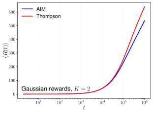
Figure 5: Temporal evolution of the regret for 2-armed bandit with Gaussian rewards ($\sigma=1$) for close mean parameters. In blue AIM, in red Thompson sampling. Arm mean reward values are fixed with $\mu_{1}=0.8$ and $\mu_{2}=0.79$, the regret is obtained by averaging over $10^{5}$ realizations.

D.5.2 Information maximization approximation for Bernoulli rewards and close arms

For completeness, we provide in Fig. 6 below regret performances in which the arms mean value are close ($\Delta\mu=0.01$) for Bernoulli reward distributions. As for Gaussian rewards, AIM shows state-of-the-art performance comparable to Thompson sampling even when arms mean rewards are difficult to distinguish.

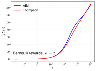
Figure 6: Temporal evolution of the regret for 2-armed bandit with Bernoulli rewards for close mean parameters. In blue AIM, in red Thompson sampling. Arm mean reward values are fixed with $\mu_{1}=0.8$ and $\mu_{2}=0.79$, the regret is obtained by averaging over $10^{5}$ realizations.

References

- Agrawal and Goyal (2013) Shipra Agrawal and Navin Goyal. Thompson Sampling for Contextual Bandits with Linear Payoffs. In Proceedings of the 30th International Conference on Machine Learning, pages 127–135. PMLR, May 2013.
- Auer (2000) P. Auer. Using upper confidence bounds for online learning. In Proceedings 41st Annual Symposium on Foundations of Computer Science, pages 270–279, Redondo Beach, CA, USA, 2000. IEEE Comput. Soc. ISBN 978-0-7695-0850-4. doi: 10.1109/SFCS.2000.892116.
- Barbier-Chebbah et al. (2023) Alex Barbier-Chebbah, Christian L. Vestergaard, and Jean-Baptiste Masson. Approximate information for efficient exploration-exploitation strategies, July 2023.
- Baudry et al. (2020) Dorian Baudry, Emilie Kaufmann, and Odalric-Ambrym Maillard. Sub-sampling for efficient non-parametric bandit exploration. In Proceedings of the 34th International Conference on Neural Information Processing Systems, NIPS’20, pages 5468–5478, Red Hook, NY, USA, December 2020. Curran Associates Inc. ISBN 978-1-71382-954-6.
- Bayati et al. (2020) Mohsen Bayati, Nima Hamidi, Ramesh Johari, and Khashayar Khosravi. Unreasonable effectiveness of greedy algorithms in multi-armed bandit with many arms. Advances in Neural Information Processing Systems, 33:1713–1723, 2020.
- Bresler et al. (2014) Guy Bresler, George H Chen, and Devavrat Shah. A latent source model for online collaborative filtering. Advances in neural information processing systems, 27, 2014.
- Bubeck et al. (2011) Sébastien Bubeck, Rémi Munos, and Gilles Stoltz. Pure exploration in finitely-armed and continuous-armed bandits. Theoretical Computer Science, 412(19):1832–1852, April 2011. ISSN 0304-3975. doi: 10.1016/j.tcs.2010.12.059.
- Cappé et al. (2013) Olivier Cappé, Aurélien Garivier, Odalric-Ambrym Maillard, Rémi Munos, and Gilles Stoltz. Kullback–Leibler upper confidence bounds for optimal sequential allocation. The Annals of Statistics, 41(3):1516–1541, June 2013. ISSN 0090-5364, 2168-8966. doi: 10.1214/13-AOS1119.
- Cardé (2021) Ring T. Cardé. Navigation Along Windborne Plumes of Pheromone and Resource-Linked Odors. Annual Review of Entomology, 66(1):317–336, 2021. doi: 10.1146/annurev-ento-011019-024932.
- Corless et al. (1996) Robert M Corless, Gaston H Gonnet, David EG Hare, David J Jeffrey, and Donald E Knuth. On the lambert w function. Advances in Computational mathematics, 5:329–359, 1996.
- Den Boer (2015) Arnoud V. Den Boer. Dynamic pricing and learning: historical origins, current research, and new directions. Surveys in operations research and management science, 20(1):1–18, 2015.
- Garivier (2013) Aurélien Garivier. Informational confidence bounds for self-normalized averages and applications. In 2013 IEEE Information Theory Workshop (ITW), pages 1–5. IEEE, 2013.
- Garivier and Cappé (2011) Aurélien Garivier and Olivier Cappé. The kl-ucb algorithm for bounded stochastic bandits and beyond. In Proceedings of the 24th annual conference on learning theory, pages 359–376. JMLR Workshop and Conference Proceedings, 2011.
- Helias and Dahmen (2020) Moritz Helias and David Dahmen. Statistical Field Theory for Neural Networks, volume 970 of Lecture Notes in Physics. Springer International Publishing, Cham, 2020. ISBN 978-3-030-46443-1 978-3-030-46444-8. doi: 10.1007/978-3-030-46444-8.
- Hernández-Lobato et al. (2015) José Miguel Hernández-Lobato, Michael A. Gelbart, Matthew W. Hoffman, Ryan P. Adams, and Zoubin Ghahramani. Predictive entropy search for Bayesian optimization with unknown constraints. In Proceedings of the 32nd International Conference on International Conference on Machine Learning - Volume 37, ICML’15, pages 1699–1707, Lille, France, July 2015. JMLR.org.
- Honda and Takemura (2010) Junya Honda and Akimichi Takemura. An Asymptotically Optimal Bandit Algorithm for Bounded Support Models. In Adam Tauman Kalai and Mehryar Mohri, editors, COLT 2010 - The 23rd Conference on Learning Theory, Haifa, Israel, June 27-29, 2010, pages 67–79. Omnipress, 2010.
- Kalyanakrishnan et al. (2012) Shivaram Kalyanakrishnan, Ambuj Tewari, Peter Auer, and Peter Stone. PAC Subset Selection in Stochastic Multi-armed Bandits. Proceedings of the 29th International Conference on Machine Learning, ICML 2012, 1, January 2012.
- Kaufmann et al. (2012a) Emilie Kaufmann, Nathaniel Korda, and Rémi Munos. Thompson sampling: An asymptotically optimal finite-time analysis. In International conference on algorithmic learning theory, pages 199–213. Springer, 2012a.
- Kaufmann et al. (2012b) Emilie Kaufmann, Nathaniel Korda, and Rémi Munos. Thompson Sampling: An Asymptotically Optimal Finite-Time Analysis. In Nader H. Bshouty, Gilles Stoltz, Nicolas Vayatis, and Thomas Zeugmann, editors, Algorithmic Learning Theory, Lecture Notes in Computer Science, pages 199–213, Berlin, Heidelberg, 2012b. Springer. ISBN 978-3-642-34106-9. doi: 10.1007/978-3-642-34106-9˙18.
- Kaufmann et al. (2016) Emilie Kaufmann, Olivier Cappé, and Aurélien Garivier. On the complexity of best-arm identification in multi-armed bandit models. J. Mach. Learn. Res., 17(1):1–42, January 2016. ISSN 1532-4435.
- Korda et al. (2013) Nathaniel Korda, Emilie Kaufmann, and Remi Munos. Thompson sampling for 1-dimensional exponential family bandits. In Proceedings of the 26th International Conference on Neural Information Processing Systems - Volume 1, NIPS’13, pages 1448–1456, Red Hook, NY, USA, December 2013. Curran Associates Inc.
- Lai et al. (1985) Tze Leung Lai, Herbert Robbins, et al. Asymptotically efficient adaptive allocation rules. Advances in applied mathematics, 6(1):4–22, 1985.
- Lee et al. (2023) Jongyeong Lee, Junya Honda, Chao-Kai Chiang, and Masashi Sugiyama. Optimality of thompson sampling with noninformative priors for pareto bandits. arXiv preprint arXiv:2302.01544, 2023.
- Li et al. (2010) Lihong Li, Wei Chu, John Langford, and Robert E Schapire. A contextual-bandit approach to personalized news article recommendation. In Proceedings of the 19th international conference on World wide web, pages 661–670, 2010.
- Locatelli et al. (2016) Andrea Locatelli, Maurilio Gutzeit, and Alexandra Carpentier. An optimal algorithm for the Thresholding Bandit Problem. In Proceedings of The 33rd International Conference on Machine Learning, pages 1690–1698. PMLR, June 2016.
- Martinez et al. (2014) Dominique Martinez, Lotfi Arhidi, Elodie Demondion, Jean-Baptiste Masson, and Philippe Lucas. Using Insect Electroantennogram Sensors on Autonomous Robots for Olfactory Searches. JoVE (Journal of Visualized Experiments), (90):e51704, August 2014. ISSN 1940-087X. doi: 10.3791/51704.
- Masson (2013) Jean-Baptiste Masson. Olfactory searches with limited space perception. Proceedings of the National Academy of Sciences, 110(28):11261–11266, July 2013. doi: 10.1073/pnas.1221091110.
- Murlis et al. (1992) John Murlis, Joseph S. Elkinton, and Ring T. Cardé. Odor Plumes and How Insects Use Them. Annual Review of Entomology, 37(1):505–532, January 1992. doi: 10.1146/annurev.en.37.010192.002445.
- Ng and Geller (1969) Edward W. Ng and Murray Geller. A table of integrals of the Error functions. J. RES. NATL. BUR. STAN. SECT. B. MATH. SCI., 73B(1):1, January 1969. ISSN 0098-8979. doi: 10.6028/jres.073B.001.
- Parr et al. (2022) Thomas Parr, Giovanni Pezzulo, and Karl J. Friston. Active Inference: The Free Energy Principle in Mind, Brain, and Behavior. The MIT Press, March 2022. ISBN 978-0-262-36997-8. doi: 10.7551/mitpress/12441.001.0001.
- Pilarski et al. (2021) Sebastian Pilarski, Slawomir Pilarski, and Dániel Varró. Optimal Policy for Bernoulli Bandits: Computation and Algorithm Gauge. IEEE Transactions on Artificial Intelligence, 2(1):2–17, February 2021. ISSN 2691-4581. doi: 10.1109/TAI.2021.3074122.
- Reddy et al. (2016) Gautam Reddy, Antonio Celani, and Massimo Vergassola. Infomax Strategies for an Optimal Balance Between Exploration and Exploitation. J Stat Phys, 163(6):1454–1476, June 2016. ISSN 1572-9613. doi: 10.1007/s10955-016-1521-0.
- Reddy et al. (2022) Gautam Reddy, Venkatesh N. Murthy, and Massimo Vergassola. Olfactory Sensing and Navigation in Turbulent Environments. Annual Review of Condensed Matter Physics, 13:191–213, March 2022. doi: 10.1146/annurev-conmatphys-031720-032754.
- Russo and Van Roy (2014) Daniel Russo and Benjamin Van Roy. Learning to Optimize via Information-Directed Sampling. In Z. Ghahramani, M. Welling, C. Cortes, N. Lawrence, and K. Q. Weinberger, editors, Advances in Neural Information Processing Systems, volume 27. Curran Associates, Inc., 2014.
- Ryzhov et al. (2012) Ilya O. Ryzhov, Warren B. Powell, and Peter I. Frazier. The Knowledge Gradient Algorithm for a General Class of Online Learning Problems. Operations Research, 60(1):180–195, February 2012. ISSN 0030-364X. doi: 10.1287/opre.1110.0999.
- Silver et al. (2016) David Silver, Aja Huang, Chris J. Maddison, Arthur Guez, Laurent Sifre, George van den Driessche, Julian Schrittwieser, Ioannis Antonoglou, Veda Panneershelvam, Marc Lanctot, Sander Dieleman, Dominik Grewe, John Nham, Nal Kalchbrenner, Ilya Sutskever, Timothy Lillicrap, Madeleine Leach, Koray Kavukcuoglu, Thore Graepel, and Demis Hassabis. Mastering the game of Go with deep neural networks and tree search. Nature, 529(7587):484–489, January 2016. ISSN 1476-4687. doi: 10.1038/nature16961.
- Thompson (1933) William R Thompson. On the likelihood that one unknown probability exceeds another in view of the evidence of two samples. Biometrika, 25(3-4):285–294, 1933.
- Tishby et al. (2000) Naftali Tishby, Fernando C. Pereira, and William Bialek. The information bottleneck method, April 2000.
- Vergassola et al. (2007) Massimo Vergassola, Emmanuel Villermaux, and Boris I. Shraiman. ‘Infotaxis’ as a strategy for searching without gradients. Nature, 445(7126):406–409, January 2007. ISSN 1476-4687. doi: 10.1038/nature05464.
- Zhang et al. (2015) Siqi Zhang, Dominique Martinez, and Jean-Baptiste Masson. Multi-Robot Searching with Sparse Binary Cues and Limited Space Perception. Frontiers in Robotics and AI, 2, 2015. ISSN 2296-9144.