Quantum teleportation implies symmetry-protected topological order

Abstract

We constrain a broad class of teleportation protocols using insights from locality. In the “standard” teleportation protocols we consider, all outcome-dependent unitaries are Pauli operators conditioned on linear functions of the measurement outcomes. We find that all such protocols involve preparing a “resource state” exhibiting symmetry-protected topological (SPT) order with Abelian protecting symmetry $\mathcal{G}_{k}=(\mathbb{Z}^{\,}_{2}\times\mathbb{Z}^{\,}_{2})^{k}$. The $k$ logical states are teleported between the edges of the chain by measuring the corresponding $2k$ string order parameters in the bulk and applying outcome-dependent Paulis. Hence, this single class of nontrivial SPT states is both necessary and sufficient for the standard teleportation of $k$ qubits. We illustrate this result with several examples, including a nonstabilizer hypergraph state.

1 Introduction

Entangled states of many-body quantum systems are valuable resources for a variety of tasks in quantum information processing. A prototypical example is quantum teleportation: By measuring an entangled state and applying unitaries conditioned on the outcomes (i.e., feedback), quantum information can be transferred over larger distances than can be achieved using unitary time evolution alone Bennett et al. (1993). Teleportation protocols can also be concatenated to form a quantum repeater that transfers quantum information over arbitrary distances Briegel et al. (1998).

It is then natural to ask what types of entangled many-body resource states can be used to teleport quantum information by measuring from one end of a 1D chain to the other and applying outcome-dependent feedback, as illustrated in Fig. 1. In fact, such entangled resource states form the backbone of many notions of quantum computation, and especially measurement-based quantum computation (MBQC), in which logical operations are applied to a quantum state as it is teleported Gottesman and Chuang (1999); Raussendorf and Briegel (2001). These same states are also closely related to the concept of localizable entanglement Popp et al. (2005), which has important connections to the ground-state properties and phase transitions of quantum spin chains Verstraete et al. (2004a, b); Jin and Korepin (2004); Pachos and Plenio (2004); Venuti and Roncaglia (2005); Skrøvseth and Bartlett (2009). Accordingly, significant effort has been invested into characterizing entangled quantum states by their utility as resources for tasks such as MBQC and quantum teleportation Raussendorf et al. (2005); Van den Nest et al. (2006); Gross and Eisert (2007); Gross et al. (2009); Bremner et al. (2009); Doherty and Bartlett (2009); Gross and Eisert (2010); Else et al. (2012); Prakash and Wei (2015); Miller and Miyake (2016); Stephen et al. (2017); Marvian (2017); Wei (2018).

Here we consider a different question. Rather than consider particular quantum states and diagnose their suitability for various quantum tasks, we instead seek to classify and constrain teleportation protocols directly, in analogy to phases of matter. The idea is to use this alternate, top-down approach to identify classes of entangled resource states compatible with teleportation. However, this requires restricting our consideration to a particular class of “standard” teleportation protocols, which include the most straightforwardly implementable protocols known to the literature. From the conditions imposed by standard teleportation, we then investigate the implications for the associated resource state.

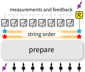
Figure 1: Illustration of the central result of this paper: All standard teleportation protocols amount to preparing an SPT state with symmetry $\mathcal{G}=\mathbb{Z}^{\,}_{2}\times\mathbb{Z}^{\,}_{2}$ with a logical state $\lvert\psi\rangle$ encoded (in purple), measuring the corresponding pair of string order parameters, and applying outcome-dependent Paulis. Teleporting $k\geq 1$ qubits requires measuring $2k$ strings.

Of particular interest is the class of many-body states in 1D with symmetry-protected topological (SPT) order Chen et al. (2011); Pollmann et al. (2010); Schuch et al. (2011); Chen et al. (2013), which are known to be useful resource states for quantum teleportation and MBQC Doherty and Bartlett (2009); Miyake (2010); Else et al. (2012); Prakash and Wei (2015); Stephen et al. (2017); Marvian (2017); Wei (2018). These states are short-range entangled, yet cannot be connected to product states via finite-depth unitaries that respect the “protecting” symmetry group $\mathcal{G}$. For an Abelian symmetry $\mathcal{G}$, the corresponding SPT states exhibit perfect long-range order characterized by nonlocal stringlike objects. These string order parameters act as commuting symmetry operators in the interior of any finite interval, but are decorated by endpoint operators at the boundaries den Nijs and Rommelse (1989); Kennedy and Tasaki (1992); Pollmann and Turner (2012). Moreover, measuring the symmetry charge in any such bulk region reduces the string order parameter to a long-range two-point correlation function of the two endpoint operators, indicating long-range entanglement that can be used for teleportation Marvian (2017). Remarkably, a state’s suitability for teleportation is a property of entire SPT phases, and not merely special points within the phase Doherty and Bartlett (2009); Else et al. (2012); Miyake (2010); Raussendorf et al. (2022), establishing a compelling link between quantum information processing and quantum phases of matter.

Another source of insight into quantum information processing is locality, which imposes bounds on the speed with which quantum information can be transferred. The Lieb-Robinson Theorem Lieb and Robinson (1972) establishes such an emergent speed limit in the context of unitary time evolution under local Hamiltonians. In fact, more general quantum channels captured by local Lindbladians obey the same bound Poulin (2010). However, when local projective measurements are combined with nonlocal feedback (via instantaneous classical signalling), the standard Lieb-Robinson bound can be overcome. Nevertheless, an alternative bound on generic useful quantum tasks has recently been derived even in the presence of nonlocal feedback Friedman et al. (2022a). These results impose optimal quantitative constraints on the distance over which qubits can be teleported.

In this paper, we use similar techniques to derive more qualitative constraints on teleportation protocols and their associated resource states. Importantly, this requires only a few physically motivated assumptions—namely that the initial state is short-range entangled and that the outcome-dependent corrections have some particular form. In particular we consider “standard” teleportation protocols, whose correction operations are Pauli gates that depend on parities of measurement outcomes. We then find that all standard teleportation protocols can be written in a particular “canonical form” that corresponds to preparing a resource state with $\mathbb{Z}_{2}^{2k}$ SPT order, measuring its string order parameters, and applying Pauli gates conditioned on the outcomes, as depicted in Fig. 1. Because such SPT states were known to be viable resource states for teleportation, our main result—captured by Theorem 18—implies an equivalence between standard teleportation and resource states with $\mathbb{Z}_{2}^{2k}$ SPT order.

This paper is organized as follows. In Sec. 2, we define important terms relevant to quantum state transfer and teleportation, review the Stinespring measurement formalism Stinespring (1955); Choi (1975); Takesaki (2012); Friedman et al. (2022b); Barberena and Friedman (2023) crucial to our analysis, along with locality bounds. In Sec. 3, we define the “standard” teleportation protocols of interest and identify several constraints on their ingredients. In Sec. 4, we use locality bounds to derive additional constraints on standard teleportation protocols. In Sec. 5, we use these constraints to obtain the main result: Standard teleportation of $k\geq 1$ logical qubits necessarily amounts to preparing a resource state with perfect $\mathbb{Z}_{2}^{2k}$ string order. In Sec. 6 we highlight these results using various examples, including states in which the SPT order is not obvious. Finally, in Sec. 7, we briefly discuss protocols beyond standard teleportation, summarize our results, and comment on future directions.

2 Teleportation overview

Here we briefly review the task of quantum teleportation. In Sec. 2.1 we identify the physical systems of interest, corresponding to qubits on a graph $G$, along with various useful operators. In Sec. 2.2, we define quantum state transfer—the measurement-free analogue of teleportation—and prove several results. In Sec. 2.3, we review the Stinespring representation Barberena and Friedman (2023); Friedman et al. (2022a, b); Stinespring (1955); Choi (1975); Takesaki (2012) of measurements and outcome-dependent operations as unitary channels on a dilated Hilbert space. In this sense, teleportation can be viewed as state transfer on the dilated Hilbert space, as we explain in Sec. 2.4, where we also consider an example of teleportation using the 1D cluster state Briegel and Raussendorf (2001), highlighting the Stinespring representation. Lastly, in Sec. 2.5, we present Theorem 2 due to Lieb and Robinson Lieb and Robinson (1972), which establishes a bound (28) on quantum state transfer. We then present Theorem 3 Friedman et al. (2022a), which extends Theorem 2 to generic quantum channels (involving measurements and nonlocal feedback) with a modified bound (29), and constrains teleportation.

2.1 Preliminaries

We consider physical systems of $N$ qubits identified with the vertices $v\in V$ of an arbitrary graph $G$. The $N$-qubit Hilbert space has the tensor-product structure

$$\mathcal{H}^{\vphantom{\prime}}_{\rm ph}=\bigotimes\limits_{v\in V}\,\mathbb{C}^{2}=\mathbb{C}^{2^{N}}\,,~{}~{}$$ (1)

and dimension $\mathcal{D}^{\,}_{\rm ph}=\operatorname*{dim}(\mathcal{H}^{\,}_{\rm ph})=2^{N}$. We denote Pauli-string operators acting on $\mathcal{H}^{\,}_{\rm ph}$ as, e.g.,

$$\Gamma^{\vphantom{\prime}}_{\boldsymbol{n}}=\bigotimes\limits_{v\in V}\,\sigma^{n^{\,}_{v}}_{v}\equiv\sigma^{\boldsymbol{n}}_{\,},~{}~{}$$ (2)

where $\boldsymbol{n}=\{\,n^{\,}_{v}\,|\,\forall\,v\in V\,\}$ is a length-$N$ vector that encodes the Pauli content $n^{\,}_{v}\in\{0,1,2,3\}$ on each vertex $v\in V$, and $\sigma^{0}_{v}\equiv\mathds{1}$, $\sigma^{1}_{j}=\sigma^{x}_{j}=X_{j}$, and so on. The $4^{N}$ unique Pauli strings form a complete, orthonormal basis for operators acting on $\mathcal{H}^{\,}_{\rm ph}$ (1); when multiplied by $\mathrm{i}^{k}$ (for $k=0,1,2,3$), these operators realize the Pauli group $\mathbf{P}^{\vphantom{*}}_{*}{N}$. Relatedly, the Clifford group $\mathbf{C}^{\vphantom{*}}_{*}{N}$ is the set of unitary operators that map the Pauli group $\mathbf{P}^{\vphantom{*}}_{*}{N}$ to itself. Note that we frequently label both the Clifford and Pauli groups by the vertex set or Hilbert space to which they correspond (e.g., $\mathbf{C}^{\vphantom{*}}_{*}{N}=\mathbf{C}^{\vphantom{*}}_{*}{V}=\mathbf{C}^{\vphantom{*}}_{*}{\rm ph}$).

Additionally, for a given $N$-qubit state $\lvert\Psi\rangle\in\mathcal{H}^{\,}_{\rm ph}$, we define the unitary stabilizer group

$$\mathcal{S}=\operatorname*{stab}\left(\lvert\Psi\rangle\right)=\left\{\,\mathsf{S}\in\mathsf{U}\left(2^{N}\right)\,\middle|\,\mathsf{S}\lvert\Psi\rangle=\lvert\Psi\rangle\,\right\}\,,~{}~{}$$ (3)

as the set of all unitaries $\mathsf{S}$ for which $\lvert\Psi\rangle$ is a $+1$ eigenstate (note that $\mathcal{S}$ always contains the identity $\mathds{1}$). Crucially, we do not require that $\mathcal{S}$ (3) be a subset of the Pauli group $\mathbf{P}^{\vphantom{*}}_{*}{N}$—i.e., we do not restrict to “stabilizer states” $\lvert\Psi\rangle$ Gottesman (1997), for which all $\mathsf{S}\in\operatorname*{stab}\left(*\right){\lvert\Psi\rangle}$ are Pauli strings (2). In fact, in Sec. 6.2, we explicitly consider teleportation protocols involving a nonstabilizer hypergraph resource state Gottesman and Chuang (1999); Rossi et al. (2013); Gachechiladze et al. (2019); Miller and Miyake (2016). Moreover, we do not require that $\mathcal{S}$ (3) be Abelian (which is guaranteed when $\mathcal{S}\subset\mathbf{P}^{\vphantom{*}}_{*}{N}$).

2.2 Quantum state transfer

Before considering quantum teleportation, we briefly discuss the related task of quantum state transfer. By convention, “quantum state transfer” refers to unitary protocols $\mathcal{W}$ applied to a system of physical qubits, while “quantum teleportation” also involves projective measurements and outcome-dependent operations (feedback).

Both tasks transfer $k\geq 1$ “logical states” within a given many-body state. A logical state is simply a particular state of a quantum bit—i.e., $\lvert\psi^{\,}_{n}\rangle=\alpha^{\,}_{n}\,\lvert 0\rangle^{\,}_{n}+\beta^{\,}_{n}\lvert 1\rangle^{\,}_{n}$ for the $n$th “logical qubit” with logical basis states $\lvert 0\rangle^{\,}_{n}$ and $\lvert 1\rangle^{\,}_{n}$. The simplest protocols $\mathcal{W}$ transfer logical states between individual physical qubits; however, logical states may also be “embedded” in many physical qubits.

Logical qubits can also be characterized in terms of their associated logical operators. If the many-body state $\lvert\Psi\rangle$ encodes $k\geq 1$ logical states $\lvert\psi^{\,}_{n}\rangle$ with coefficients $\alpha^{\,}_{n},\beta^{\,}_{n}$ (for $1\leq n\leq k$), then the corresponding logical basis operators $X^{(n)}_{{\rm L}},Y^{(n)}_{{\rm L}},Z^{(n)}_{{\rm L}}$ are defined such that,

$$\left\langle*\middle|\Psi\middle|X^{(n)}_{{\rm L}}\right\rangle{\Psi} =\left\langle*\middle|\psi^{\vphantom{\prime}}_{n}\middle|X^{\vphantom{*}}\right\rangle{\psi^{\vphantom{\prime}}_{n}}=2\,\mathrm{Re}(\alpha^{*}_{n}\beta^{\vphantom{\prime}}_{n})$$ (4a)

$$\left\langle*\middle|\Psi\middle|Y^{(n)}_{{\rm L}}\right\rangle{\Psi} =\left\langle*\middle|\psi^{\vphantom{\prime}}_{n}\middle|Y^{\vphantom{*}}\right\rangle{\psi^{\vphantom{\prime}}_{n}}=2\,\mathrm{Im}(\beta^{*}_{n}\alpha^{\vphantom{\prime}}_{n})$$ (4b)

$$\left\langle*\middle|\Psi\middle|Z^{(n)}_{{\rm L}}\right\rangle{\Psi} =\left\langle*\middle|\psi^{\vphantom{\prime}}_{n}\middle|Z^{\vphantom{*}}\right\rangle{\psi^{\vphantom{\prime}}_{n}}=\lvert\alpha^{\vphantom{\prime}}_{n}\rvert^{2}-\lvert\beta^{\vphantom{\prime}}_{n}\rvert^{2}\,,~{}~{}$$ (4c)

so that the logical Paulis $X^{(n)}_{{\rm L}},Y^{(n)}_{{\rm L}},Z^{(n)}_{{\rm L}}$ span all logical operations on the $n$th logical qubit.

In general, the logical operators must reproduce the Pauli algebra and satisfy Eq. 4. However, in the context of state transfer and teleportation, we assume that the initial and final many-body states are separable with respect to the $k$ logical qubits and all other physical qubits, and realized on $k$ physical sites. Often, the $n$th logical qubit is realized on the physical qubit $j$, so that $X^{(n)}_{{\rm L}},Y^{(n)}_{{\rm L}},Z^{(n)}_{{\rm L}}$ reduce to the standard Paulis $X^{\vphantom{*}}_{j}$, $Y^{\vphantom{*}}_{j}$, and $Z^{\vphantom{*}}_{j}$.

Definition 1.

A unitary protocol $\mathcal{W}$ acting on $\mathcal{H}^{\,}_{\rm ph}$ (1) achieves quantum state transfer of $k$ logical qubits from the initial logical vertex set $I=\{i_{1},\dots,i_{k}\}\subset V$ to the final logical vertex set $F=\{f_{1},\dots,f_{k}\}\subset V$ if

$$\lvert\Psi^{\vphantom{\prime}}_{T}\left(\boldsymbol{\alpha},\boldsymbol{\beta}\right)\rangle=\mathcal{W}\,\lvert\Psi^{\vphantom{\prime}}_{0}\left(\boldsymbol{\alpha},\boldsymbol{\beta}\right)\rangle\,,~{}~{}$$ (5)

with the initial and final states given by

$$\lvert\Psi^{\vphantom{\prime}}_{0}\left(\boldsymbol{\alpha},\boldsymbol{\beta}\right)\rangle =\left[\bigotimes\limits_{n=1}^{k}\,\lvert\psi^{\vphantom{*}}_{n}(\alpha^{\vphantom{*}}_{n},\beta^{\vphantom{*}}_{n})\rangle^{\vphantom{\dagger}}_{i_{n}}\right]\otimes\lvert\Phi^{\vphantom{\prime}}_{0}\rangle^{\vphantom{\dagger}}_{I^{c}}$$ (6)

$$\lvert\Psi^{\vphantom{\prime}}_{T}\left(\boldsymbol{\alpha},\boldsymbol{\beta}\right)\rangle =\left[\bigotimes\limits_{n=1}^{k}\,\lvert\psi^{\vphantom{*}}_{n}(\alpha^{\vphantom{*}}_{n},\beta^{\vphantom{*}}_{n})\rangle^{\vphantom{\dagger}}_{f_{n}}\right]\otimes\lvert\Phi^{\vphantom{\prime}}_{T}\rangle^{\vphantom{\dagger}}_{F^{c}}\,,~{}$$ (7)

where the logical state $\lvert\psi^{\,}_{n}\rangle=\alpha^{\,}_{n}\lvert 0\rangle+\beta^{\,}_{n}\lvert 1\rangle$ is transferred from site $i^{\,}_{n}\in I$ (6) to site $f^{\,}_{n}\in F$ (7), $\boldsymbol{\alpha}=(\alpha^{\,}_{1},\dots,\alpha^{\,}_{k})$ and $\boldsymbol{\beta}=(\beta^{\,}_{1},\dots,\beta^{\,}_{k})$ satisfy $\lvert\alpha^{\,}_{n}\rvert^{2}+\lvert\beta^{\,}_{n}\rvert^{2}=1$ for each $n$, and $\lvert\Phi^{\,}_{0}\rangle$ and $\lvert\Phi^{\,}_{T}\rangle$ are arbitrary many-body states on the $N-k$ qubits in $I^{c}$ and $F^{c}$, respectively.

We now present Prop. 1, which establishes necessary and sufficient conditions for quantum state transfer in terms of logical and stabilizer operators, an equivalence between the transfer of logical states and logical operators, and that the logical operators in the initial and final many-body states are spanned by the Pauli operators $X^{\vphantom{*}}_{i_{n}},Z^{\vphantom{*}}_{i_{n}}$ and $X^{\vphantom{*}}_{f_{n}},Z^{\vphantom{*}}_{f_{n}}$, for $i^{\,}_{n}\in I$ and $f^{\,}_{n}\in F$, respectively.

Proposition 1 (State-transfer conditions).

Given an initial state of the form (6), the following conditions are necessary and sufficient for a unitary protocol $\mathcal{W}$ to achieve quantum state transfer of $k$ logical states $\lvert\psi^{\,}_{n}\rangle$,

$$\mathcal{W}^{\dagger}X^{\vphantom{*}}_{f_{n}}\mathcal{W} =X^{\vphantom{*}}_{i_{n}}\,\mathsf{S}_{n,x}$$ (8a)

$$\mathcal{W}^{\dagger}Z^{\vphantom{*}}_{f_{n}}\mathcal{W} =Z^{\vphantom{*}}_{i_{n}}\,\mathsf{S}_{n,z}\,,$$ (8b)

for $1\leq n\leq k$, where $\mathsf{S}_{n,\nu}\in\operatorname*{stab}\left(\lvert\Psi^{\,}_{0}\rangle\right)$ (3) are unitary and stabilize $\lvert\Psi^{\,}_{0}\rangle$ (6); see also Def. 1.

The proof of Prop. 1 appears in App. A. Loosely speaking, Prop. 1 establishes that the task of transferring $k$ logical states from the logical sites $I=\{i_{1},\dots,i_{k}\}\subset V$ to the logical sites $F=\{f_{1},\dots,f_{k}\}\subset V$ in the Schrödinger picture is equivalent to transferring $k$ pairs of $X$- and $Z$-type logical operators from the logical sites in $F$ to those in $I$ in the Heisenberg picture. The result for the $n$th $Y$-type logical operator follows from $Y^{\vphantom{*}}=\mathrm{i}X^{\vphantom{*}}Z^{\vphantom{*}}$:

$$\mathcal{W}^{\dagger}Y^{\vphantom{*}}_{f_{n}}\mathcal{W} =Y^{\vphantom{*}}_{i_{n}}\,\mathsf{S}_{n,y}\,,$$ (9)

where $\mathsf{S}_{n,y}\equiv Z^{\vphantom{*}}_{i_{n}}\mathsf{S}_{n,x}Z^{\vphantom{*}}_{i_{n}}\mathsf{S}_{n,z}\in\operatorname*{stab}\left(\lvert\Psi^{\vphantom{*}}_{0}\rangle\right)$.

Importantly the result (8) of Prop. 1 captures how any logical operation $\mathcal{O}^{\,}_{n}$ on the $n$th logical qubit in the final state $\lvert\Psi^{\,}_{T}\rangle$ (7) is related to the same logical operation $\mathcal{O}^{\,}_{n}$ on the $n$th logical qubit in the initial state $\lvert\Psi^{\,}_{0}\rangle$ (6). Since the logical Paulis $\sigma^{\nu}_{n,{\rm L}}$ for $\nu=1,2,3$ form a complete basis for $\mathcal{O}^{\,}_{n}$ in the final state $\lvert\Psi^{\,}_{T}\rangle$ (7), Prop. 1 implies that

$$O^{\vphantom{\prime}}_{f_{n}}(T) =\mathcal{W}^{\dagger}\,O^{\vphantom{\prime}}_{f_{n}}\mathcal{W}$$

$$=\frac{1}{2}\sum\limits_{\nu=0}^{3}\,\operatorname*{tr}\limits_{f_{n}}\left[O^{\vphantom{\prime}}_{f_{n}}\,\sigma^{\nu}_{f_{n}}\right]\,\mathcal{W}^{\dagger}\,\sigma^{\nu}_{f_{n}}\,\mathcal{W}$$

$$=\frac{1}{2}\sum\limits_{\nu=1}^{3}\,\operatorname*{tr}\limits_{i_{n}}\left[O^{\vphantom{\prime}}_{i_{n}}\,\sigma^{\nu}_{i_{n}}\right]\,\sigma^{\nu}_{i_{n}}\,\mathsf{S}_{n,\nu}$$

$$\equiv O^{\vphantom{\prime}}_{i_{n}}\mathsf{S}_{n,O}\,,$$ (10)

is equivalent to $O^{\,}_{i_{n}}$ acting on $\lvert\Psi^{\,}_{0}\rangle$ (6).

Prop. 1 establishes that state transfer requires growing the support of logical operators. Quantitatively, the degree of “overlap” between two operators can be captured by commutator norms. To this end, we define the standard spectral norm of an operator as

$$\lVert A\rVert\equiv\max\limits_{\lambda\in{\rm eigs}(A)}\,\lvert\lambda\rvert\,,~{}~{}$$ (11)

which is magnitude of the largest eigenvalue of $A$. Using the fact that $\lVert\left\{\sigma^{\nu}_{n,{\rm L}},\,\mathsf{S}\right\}\rVert=2$, we find that Friedman et al. (2022a)

$$\lVert\left[\mathcal{W}^{\dagger}X^{\vphantom{*}}_{f_{n}}\mathcal{W},\,Z^{\vphantom{*}}_{i_{n}}\right]\rVert=2\,,$$ (12)

meaning that successful state transfer implies that the Heisenberg-evolved logical operator $X^{\vphantom{*}}_{f_{n}}(T)$ for the $n$th logical qubit realizes the operator $X^{\vphantom{*}}_{i_{n}}$ acting on the initial state, and obeys the Pauli algebra (12).

Finally, we define the “task distance” $L$ for quantum state transfer (and later, teleportation), as the minimum distance any logical qubit is transferred.

Definition 2.

The task distance (or teleportation distance) for a protocol $\mathcal{W}$ that maps the initial state $\lvert\Psi^{\,}_{0}\rangle$ (6) with $k$ logical qubits on the sites $I=\{i_{1},i_{2},\dots,i_{k}\}\subset V$ to the state $\lvert\Psi^{\,}_{T}\rangle$ (7) with logical qubits on the sites $F=\{f_{1},f_{2},\dots,f_{k}\}\subset V$ is given by

$$L\equiv\min\limits_{n}\,d(i_{n},f_{n})\,,~{}~{}$$ (13)

where the metric $d(x,y)$ is defined by the graph $G$.

2.3 Stinespring measurement

To facilitate our discussion of quantum teleportation—which involves measurements and outcome-dependent feedback—we now review the Stinespring formalism Friedman et al. (2022a, b); Barberena and Friedman (2023); Stinespring (1955), which derives from the Stinespring Dilation Theorem Stinespring (1955); Choi (1975); Takesaki (2012). The formalism leads to a unitary representation of projective measurements and outcome-dependent operations in a dilated Hilbert space,

$$\mathcal{H}^{\vphantom{\dagger}}_{\rm dil}\equiv\mathcal{H}^{\vphantom{\dagger}}_{\rm ph}\otimes\mathcal{H}^{\vphantom{\dagger}}_{\rm ss}\,,~{}~{}$$ (14)

where $\mathcal{H}^{\,}_{\rm ph}$ is the physical Hilbert space (1) and $\mathcal{H}^{\,}_{\rm ss}$ is the “Stinespring” Hilbert space. For a protocol $\mathcal{W}$ involving $M$ single-qubit measurements, $\mathcal{H}^{\,}_{\rm ss}=\mathbb{C}^{2M}$ contains $M$ qubits, which store the $M$ outcomes (and reflect the states of the corresponding measurement apparati).

The crucial result of the Stinespring Theorem Stinespring (1955); Takesaki (2012); Choi (1975) in this context is that all valid quantum channels (i.e., positive maps) can be represented via isometries. An isometry is a map $\mathbb{V}\,:\,\mathcal{H}\to\mathcal{H}^{\prime}$, where $\mathcal{D}\leq\mathcal{D}^{\prime}$. When $\mathcal{D}=\mathcal{D}^{\prime}$, $\mathbb{V}$ is a unitary; when $\mathcal{D}<\mathcal{D}^{\prime}$, $\mathbb{V}$ dilates $\mathcal{H}$ to $\mathcal{H}^{\prime}=\mathcal{H}^{\,}_{\rm dil}$ (14). Crucially, one can always embed the isometry $\mathbb{V}\,:\,\mathcal{H}^{\,}_{\rm ph}\to\mathcal{H}^{\,}_{\rm dil}$ in a unitary $U\,:\,\mathcal{H}^{\,}_{\rm dil}\to\mathcal{H}^{\,}_{\rm dil}$ by working in $\mathcal{H}^{\,}_{\rm dil}$ from the outset; this merely requires identifying a default initial state of all measurement apparati, which we take to be $\lvert 0\rangle^{\,}_{\rm ss}$ without loss of generality Takesaki (2012); Choi (1975); Friedman et al. (2022b, a); Stinespring (1955); Barberena and Friedman (2023).

We first consider the Stinespring representation of projective measurements. An observable $A$ with $\mathcal{N}$ unique eigenvalues $a^{\,}_{n}$ has a spectral decomposition given by

$$A =\sum\limits_{n=0}^{\mathcal{N}-1}\,a^{\vphantom{\prime}}_{n}\,P^{(n)}_{A}\,,~{}~{}$$ (15)

where the projectors are orthogonal, idemptotent, and complete. The trace of each projector is equal to the degeneracy of the corresponding eigenvalue. The dilated unitary channel that captures measurement of $A$ (15) is

$$\mathcal{M}^{\vphantom{\dagger}}_{\left[A\right]} =\sum\limits_{m,n=0}^{\mathcal{N}-1}\,P^{(m)}_{A}\otimes\lvert n+m\rangle\langle n\rvert^{\vphantom{\prime}}_{\rm ss}\,,~{}~{}$$ (16)

which is unique up to the definition of the Stinespring basis and choice of default state Stinespring (1955); Takesaki (2012); Friedman et al. (2022b, a); Barberena and Friedman (2023); Choi (1975). Projecting the post-measurement state onto the $n$th Stinespring state leads to the physical state $\lvert\psi^{\prime}\rangle\propto P^{(n)}_{A}\,\lvert\psi\rangle$ (15), as required. For example, when $A=Z^{\vphantom{*}}_{j}$, we have

$$\mathcal{M}^{\vphantom{\dagger}}_{\left[Z^{\vphantom{*}}_{j}\right]} =\frac{1}{2}\sum\limits_{m=0,1}\left(\mathds{1}+(-1)^{m}\,Z^{\vphantom{*}}_{j}\right)\otimes\widetilde{X}^{m}_{j}~{}~{}$$

$$=P^{(0)}_{j}\otimes\widetilde{\mathds{1}}^{\vphantom{*}}_{j}+P^{(1)}_{j}\otimes\widetilde{X}^{\,}_{j},$$ (17)

which is simply a CNOT gate from the physical site $j$ to the Stinespring qubit $j$. In general, we use tildes to denote operators on the Stinespring registers, which we label according to the corresponding observable.

The Stinespring formalism also represents outcome-dependent operations as controlled unitary operations on the physical qubits, conditioned on the Stinespring qubits. Since we assume classical communication (of the outcomes) to be instantaneous, such operations may be conditioned on any prior outcomes (in the Schrödinger picture), and take the generic form

$$\mathcal{R}^{\vphantom{\dagger}}_{\Omega} =\sum\limits_{\boldsymbol{n}}\,\chi^{\vphantom{\dagger}}_{\boldsymbol{n}}\otimes\widetilde{P}^{(\boldsymbol{n})}_{\Omega}\,,~{}~{}$$ (18)

where $\widetilde{P}^{(\boldsymbol{n})}_{\Omega}$ is an $\widetilde{Z}^{\vphantom{*}}$-basis projector onto the outcome “trajectory” $\boldsymbol{n}=(n^{\,}_{1},\dots,n^{\,}_{s})$ for the subset $\Omega\subset V^{\,}_{\rm ss}$. The “recovery operators” $\chi^{\,}_{\boldsymbol{n}}$ must act unitarily on $\mathcal{H}^{\,}_{\rm ph}$ and/or any unused Stinespring registers. For example, one might apply $X^{\vphantom{*}}_{i}$ to the physical qubit $i$ if the $j$th outcome was $-1$, and do nothing otherwise, so that $\mathcal{R}^{\,}_{\Omega}$ (18) becomes

$$\mathcal{R}^{\vphantom{\dagger}}_{j\to i} =\mathds{1}^{\vphantom{\dagger}}_{i}\otimes\widetilde{P}^{(0)}_{j}+X^{\vphantom{*}}_{i}\otimes\widetilde{P}^{(1)}_{j}\,,~{}~{}$$ (19)

which is simply a CNOT gate from the Stinespring site $j$ to the physical qubit $i$, in contrast to $\mathcal{M}^{\,}_{[Z]}$(2.3).

2.4 Physical teleportation

We are now equipped to define quantum teleportation in a general sense. Importantly, we distinguish this notion of physical teleportation—as described in Def. 3—from the slightly restricted class of quantum teleportation protocols we consider later on. We then consider a canonical example teleportation protocol involving the 1D cluster state Briegel and Raussendorf (2001); the corresponding circuit is depicted in Fig. 2.

Definition 3.

Physical teleportation refers to any unitary protocol $\mathcal{W}$ acting on a dilated Hilbert space $\mathcal{H}^{\,}_{\rm dil}$ (14) that (i) fulfills the criteria for quantum state transfer (see Def. 1) and (ii) involves the combination of $M>1$ measurements, instantaneous classical communication, and outcome-dependent operations.

We stress that physical teleportation requires that the $k$ logical qubits be localized to $k$ physical qubits both before and after the protocol $\mathcal{W}$. This is in contrast to more general definitions of teleportation—which we refer to as “virtual teleportation”—in which the logical qubits may be spread out amongst many physical qubits, but can nonetheless be decoded using certain measurements thereof. This is the case for general teleportation protocols based on matrix product states Gross and Eisert (2007); Else et al. (2012); we relegate the treatment of virtual teleportation to future work Hong et al. (2023).

Importantly, the class of teleportation protocols described by Def. 3 is too broad to constrain. However, as far as we are aware, all known physical teleportation protocols—in which the final state is of the form $\lvert\Psi^{\,}_{T}\rangle$ (7)—belong to a slightly restricted class of protocols. Before defining that class in Sec. 3, we briefly consider a canonical example protocol belonging to this class (depicted in Fig. 2 for $N=5$ qubits) based on the 1D cluster state Briegel and Raussendorf (2001) that teleports a single logical qubit.

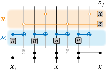
Figure 2: Dilated quantum circuit for 1D cluster-state teleportation of a single logical qubit a distance $L=4$, along with Heisenberg evolution of the logical $X_{\rm L}$ operator. The $M=4$ Stinespring qubits are depicted in gray, the measurement channel in blue, and the outcome-dependent operations in orange (the operation on site $f=5$ is conditioned on the parity of the Stinespring qubits, indicated by white circles). The initial state is given by (20), with $\lvert\psi\rangle$ on the leftmost site, so that $X_{\rm L}(T)=X_{1}X_{3}X_{5}$ is a valid logical operator.

The initial state is the product state

$$\lvert\Psi^{\vphantom{*}}_{0}\rangle=\lvert\psi\rangle^{\vphantom{\prime}}_{1}\otimes\lvert+++\dots\rangle^{\vphantom{\prime}}_{\rm rest}\otimes\lvert\boldsymbol{0}\rangle^{\vphantom{\prime}}_{\rm ss}\,,~{}~{}$$ (20)

where $\lvert+\rangle$ is the $+1$ eigenstate of $X^{\vphantom{*}}$, $\lvert\boldsymbol{0}\rangle=\lvert 0\cdots 0\rangle$ is the default Stinespring state, and we take $N$ to be odd. We first apply to $\lvert\Psi^{\,}_{0}\rangle$ (20) the (physical) unitary circuit

$$\mathcal{U}=\prod_{j=1}^{N-1}\mathrm{CZ}^{\vphantom{*}}_{j,j+1}\,,$$ (21)

where the controlled-$Z^{\vphantom{*}}$ gate $\mathrm{CZ}=\mathrm{diag}(1,1,1,-1)$ in the two-qubit computational ($Z^{\vphantom{*}}$) basis. Applying $\mathcal{U}$ to $\lvert\Psi^{\vphantom{*}}_{0}\rangle$ prepares the so-called cluster state Briegel and Raussendorf (2001).

We then measure $X^{\vphantom{*}}$ on all sites $j=1,\dots,N-1$ (where $i=1$ and $f=N$ are the initial and final logical sites, respectively). This is represented by the measurement channel $\mathcal{M}$, corresponding to the blue-shaded region of Fig. 2, which is the product of the channels

$$\mathcal{M}^{\vphantom{\dagger}}_{j}=P^{(+)}_{j}\otimes\widetilde{\mathds{1}}^{\vphantom{*}}_{j}+P^{(-)}_{j}\otimes\widetilde{X}^{\vphantom{*}}_{j}\,,~{}~{}$$ (22)

where the projectors are in the $X^{\vphantom{*}}_{j}$ basis, and the Stinespring registers are marked in light gray in Fig. 2.

Finally, we apply the outcome-dependent recovery operations. The parity of outcomes on “odd” sites $j=2n+1$ (with $j<N$) determines a final $Z^{\vphantom{*}}_{N}$ rotation, while the parity of outcomes on “even” sites $j=2n+2$ (with $j<N)$ determines a final $X^{\vphantom{*}}_{f}=X^{\vphantom{*}}_{N}$ rotation, according to

$$\mathcal{R}^{\vphantom{\dagger}}_{z} =\mathds{1}^{\vphantom{\dagger}}_{f}\otimes\widetilde{P}^{(0)}_{\rm even}+X^{\vphantom{*}}_{f}\otimes\widetilde{P}^{(1)}_{\rm even}$$ (23a)

$$\mathcal{R}^{\vphantom{\dagger}}_{x} =\mathds{1}^{\vphantom{\dagger}}_{f}\otimes\widetilde{P}^{(0)}_{\rm odd}+Z^{\vphantom{*}}_{f}\otimes\widetilde{P}^{(1)}_{\rm odd}\,,$$ (23b)

where, e.g., $\widetilde{P}^{(n)}_{\rm even}$ projects onto the parity-$n$ configuration $\widetilde{Z}^{\vphantom{*}}_{\rm even}=(-1)^{n}$ of the even Stinespring qubits. The channels above appear in the orange-shaded part of Fig. 2; they are named according to the logical operator they modify, and may be applied in either order. After applying these three steps, the initial logical state $\lvert\psi\rangle$ appears on site $f$ for any sequence of measurement outcomes.

Having defined the cluster-state teleportation protocol $\mathcal{W}$, we can evolve the final-state logical operator $X^{\vphantom{*}}_{{\rm L}}=X^{\vphantom{*}}_{f}$ backwards in time via the Heisenberg picture. We have

$$\mathcal{R}^{\dagger}X^{\vphantom{*}}_{f}\mathcal{R} =\mathcal{R}^{\dagger}_{x}X^{\vphantom{*}}_{f}\mathcal{R}^{\vphantom{\dagger}}_{x}=X^{\vphantom{*}}_{f}\prod_{j=1}^{L/2}\widetilde{Z}^{\vphantom{*}}_{2j-1}$$ (24a)

$$\mathcal{R}^{\dagger}Z^{\vphantom{*}}_{f}\mathcal{R} =\mathcal{R}^{\dagger}_{z}Z^{\vphantom{*}}_{f}\mathcal{R}^{\vphantom{\dagger}}_{z}=Z^{\vphantom{*}}_{f}\,\prod_{j=1}^{L/2}\widetilde{Z}^{\vphantom{*}}_{2j}\,,~{}~{}$$ (24b)

where $L=N-1$. Next, evolving through $\mathcal{M}$ gives

$$\mathcal{M}^{\dagger}\mathcal{R}^{\dagger}X^{\vphantom{*}}_{f}\mathcal{R}\mathcal{M} =X^{\vphantom{*}}_{f}\,\prod_{j=1}^{L/2}X^{\vphantom{*}}_{2j-1}\,\widetilde{Z}^{\vphantom{*}}_{2j-1}$$ (25a)

$$\mathcal{M}^{\dagger}\mathcal{R}^{\dagger}Z^{\vphantom{*}}_{f}\mathcal{R}\mathcal{M} =Z^{\vphantom{*}}_{f}\,\prod_{j=1}^{L/2}X^{\vphantom{*}}_{2j}\,\widetilde{Z}^{\vphantom{*}}_{2j}\,,~{}~{}$$ (25b)

and evolving through the circuit $\mathcal{U}$ (21) leads to

$$\mathcal{W}^{\dagger}X^{\vphantom{*}}_{f}\mathcal{W} =X^{\vphantom{*}}_{i}\,\underbrace{\prod_{j=1}^{L/2}X^{\vphantom{*}}_{2j+1}\,\widetilde{Z}^{\vphantom{*}}_{2j-1}}_{\mathsf{S}_{x}}$$ (26a)

$$\mathcal{W}^{\dagger}Z^{\vphantom{*}}_{f}\mathcal{W} =Z^{\vphantom{*}}_{i}\,\underbrace{\prod_{j=1}^{L/2}X^{\vphantom{*}}_{2j}\,\widetilde{Z}^{\vphantom{*}}_{2j}}_{\mathsf{S}_{z}}\,,~{}~{}$$ (26b)

from which we identify $\mathsf{S}^{\,}_{x}$ and $\mathsf{S}^{\,}_{z}$ according to Prop. 1, and confirm that they indeed stabilize $\lvert\Psi^{\,}_{0}\rangle$ (20).

We now comment on several properties of the foregoing protocol. Observe that there are effectively two types of commuting measurements, corresponding to even versus odd sites. There are also two types of recovery channel—one for each logical operator—which depend only on the measurement outcomes on the even sites and odd sites, respectively. Finally, if we take the stabilizers $\mathsf{S}_{x}$ and $\mathsf{S}_{z}$ and evolve them forwards through $\mathcal{U}$, we find

$$\mathcal{U}\,\mathsf{S}^{\vphantom{\prime}}_{x}\,\mathcal{U}^{\dagger} =Z^{\vphantom{*}}_{2}\left(\prod_{j=2}^{L/2}X^{\vphantom{*}}_{2j-1}\right)X^{\vphantom{*}}_{N}$$ (27a)

$$\mathcal{U}\,\mathsf{S}^{\vphantom{\prime}}_{z}\,\mathcal{U}^{\dagger} =Z^{\vphantom{*}}_{1}X^{\vphantom{*}}_{2}\left(\prod_{j=2}^{L/2}X^{\vphantom{*}}_{2j}\right)Z^{\vphantom{*}}_{N},~{}~{}$$ (27b)

up to $\widetilde{Z}^{\vphantom{*}}$ operators, which we recognize as the string order parameters of the cluster state Briegel and Raussendorf (2001). Observe that, while these operators necessarily commute in the bulk of the chain, the endpoint operators anticommute—i.e., $\{Z^{\vphantom{*}}_{2},Z^{\vphantom{*}}_{1}X^{\vphantom{*}}_{2}\}=\{X^{\vphantom{*}}_{N},Z^{\vphantom{*}}_{N}\}=0$. This anticommutation demonstrates the nontrivial SPT order of the cluster state, as we discuss in further detail in Sec. 5.1.

In the remainder, we prove that many of the above features—including the emergence of string order parameters for the state to which $\mathcal{M}$ is applied—are ubiquitous features of a large class of teleportation protocols.

2.5 Bounds on teleportation

Before defining a restricted class of teleportation protocols in Sec. 3, we briefly discuss general bounds on generic useful quantum tasks that derive from locality. We first consider bounds for unitary protocols $\mathcal{W}=\mathcal{U}$ (e.g., state transfer) that act only on $\mathcal{H}^{\,}_{\rm ph}$ (1). In general, we regard $\mathcal{U}$ as a finite-depth quantum circuit (FDQC), though all of our results are compatible with $\mathcal{U}$ being generated by evolution under a local Hamiltonian, up to exponentially small operator tails. In either case, the task distance $L$ (13) obeys the Lieb-Robinson Theorem Lieb and Robinson (1972), which we state below as Theorem 2.

Theorem 2 (Lieb Robinson Lieb and Robinson (1972)).

Consider a unitary $\mathcal{W}$ realizing time evolution on $\mathcal{H}^{\,}_{\rm ph}$ (1) for total time $T$, and two operators $A$ and $B$ with support in regions $X$ and $Y$, where $\lVert A\rVert=\lVert B\rVert=1$ (11) and $d(X,Y)=L$. Then,

$$\lVert\left[\,\mathcal{W}^{\dagger}A\,\mathcal{W}\,,\,B\right]\rVert\lesssim e^{v\,T-L}\,,~{}~{}$$ (28)

where the Lieb-Robinson velocity $v$ depends on $\mathcal{W}$ and the graph $G$, and the inequality is exact in the limit $L,T\gg 1$.

Theorem 2 has been proven in the literature for numerous classes of local Hamiltonians (and circuits) Lieb and Robinson (1972); Hastings (2010); Wang and Hazzard (2020). It has also been extended to long-range interactions Foss-Feig et al. (2015); Chen and Lucas (2019); Kuwahara and Saito (2020); Tran et al. (2020) and even local Lindblad dynamics Poulin (2010), up to minor modifications to the Lieb-Robinson velocity $v$. In the case of dynamics generated by local quantum circuits, the linear “light cone” is sharp, in that the commutator norm (28) is identically zero until $vT\geq L$, after which it is $\mathsf{O}\left(1\right)$. Detailed reviews of Lieb-Robinson bounds and their applications appear in, e.g., Refs. 47 and 53.

In the context of teleportation, the use of projective measurements and outcome-dependent operations far from the corresponding measurement can realize a task distance $L$ (13) that exceeds the Lieb-Robinson bound (28). However, strictly local nonunitary channels are captured by Lindblad dynamics, and obey the same Lieb-Robinson bound (28) Poulin (2010); hence, such channels are not useful to teleportation (compared to time evolution alone), and we do not consider them herein. Although teleportation can overcome the conventional Lieb-Robinson bound (28), it is nonetheless constrained by an alternative bound due to Ref. 36, which we now state in the specific context of teleporting $k$ qubits as Theorem 3.

Theorem 3 (Teleportation bound Friedman et al. (2022a)).

Consider a protocol $\mathcal{W}$ involving (i) unitary time evolution generated by a local Hamiltonian $H(t)$ for duration $T$, (ii) $M$ local projective measurements, and (iii) arbitrary local operations based all prior measurement outcomes. If $\mathcal{W}$ teleports $k$ logical states (per Def. 6) or generates $k$ bits of entanglement, then the task distance $L$ (13) obeys the bound

$$L\leq 2\left(1+\left\lfloor\frac{M}{k}\right\rfloor\right)v\,T\,,~{}~{}$$ (29)

where $v$ is determined solely by the Hamiltonian $H$ that generates time evolution in $\mathcal{W}$. If $\mathcal{W}$ is a circuit, then $T$ is the circuit depth and $v$ is the maximum distance between any two qubits acted upon by a single gate.

While the teleportation bound (29) depends on the number of measurements $M$, the general bounds of Ref. 36 depend on the number of “measurement regions” $m$ (see Sec. 4.3). Teleporting a single qubit ($k=1$), e.g., obeys

$$L\leq 2\left(m+1\right)vT\,,~{}~{}$$ (30)

and we prove in Sec. 4 for all $k\geq 1$ that standard teleportation protocols require $M=2k$ outcomes per “region,” so the factor of two in the bound (29) is loose. In fact, it was conjectured in Ref. 36 that a minimum of two distinct measurements are required per logical qubit, per measurement region. By comparison, generating long-range entanglement—e.g., preparing an $N$-qubit Greenberger-Horne-Zeilinger (GHZ) state Greenberger et al. (1989); Piroli et al. (2021)—may succeed with a single measurement per region.

The bounds of Ref. 36 apply to generic quantum tasks that transfer or generate quantum information, entanglement, and/or correlations using arbitrary local quantum channels and instantaneous classical communication. Even when gates are conditions on the outcomes of arbitrarily distant measurements, a finite speed limit emerges. While all such protocols obey the generalized bound (30), only protocols involving local time evolution, projective measurements, and outcome-dependent feedback are compatible with violations of the standard Lieb-Robinson bound (28) Poulin (2010); Friedman et al. (2022a)—and thus, teleportation.

3 Protocols of interest

Here we detail the physical teleportation protocols of interest, motivated both by practical constraints and analytical necessity, culminating in Def. 6 in Sec. 3.4. Importantly, the “standard teleportation protocols” captured by Def. 6 include all known physical teleportation protocols.

3.1 Canonical form

Here we define the canonical form $\mathcal{W}$ of a measurement-based protocol $\mathcal{W}^{\prime}$. We note that physical unitaries $U$ that act after a dilated channel (i.e., $\mathcal{R}_{j}^{\prime}$ or $\mathcal{M}_{j}^{\prime}$) can always be “pulled through” to act before that channel, at the cost of modifying the latter according to $U\mathcal{R}_{j}^{\prime}=\mathcal{R}^{\vphantom{\prime}}_{j}U$, where $\mathcal{R}^{\vphantom{\prime}}_{j}=U\mathcal{R}_{j}^{\prime}U^{\dagger}$, and likewise for $\mathcal{M}_{j}^{\prime}$. See Fig. 3.

Definition 4.

The canonical form $\mathcal{W}$ of the naïve protocol $\mathcal{W}^{\prime}$ involving physical unitaries, projective measurements, and outcome-dependent operations is given by

$$\mathcal{W}=\mathcal{R}\,\mathcal{M}\,\mathcal{U}\,,~{}~{}$$ (31)

where $\mathcal{U}$ includes all physical unitaries, $\mathcal{M}$ includes all measurements, and $\mathcal{R}$ includes all recovery operations.

We now briefly comment on Def. 4. Crucially, $\mathcal{W}$ and $\mathcal{W}^{\prime}$ are mathematically and physically the same protocol (i.e., $\mathcal{W}=\mathcal{W}^{\prime}$). However, the effective measured observables $A^{\,}_{j}$ and recovery operators $\chi^{\,}_{j}$ in $\mathcal{W}$ may differ from those in the naïve protocol $\mathcal{W}^{\prime}$. The canonical form (31) is essential to defining the class of protocols of interest and numerous other results. Additionally, familiar teleportation protocols (such as the cluster-state example in Sec. 2.4) already realize the canonical form (31).

However, by identifying modified channels as needed, any protocol $\mathcal{W}^{\prime}$ whose projective measurements are effectively instantaneous and whose recovery operations effectively realize a quantum circuit can be rewritten in canonical form $\mathcal{W}$ (31). The unitary operations captured by $\mathcal{U}$ may be generated by evolution under a local, time-dependent Hamiltonian. Using, e.g., the interaction picture, the corresponding unitaries can be “pulled through” the measurement channels and recovery operations without complication, because the latter are effectively instantaneous Friedman et al. (2022a). We note that, in the presence of outcome-dependent measurements, one also includes in $\mathcal{W}$ (31) a channel $\mathcal{M}^{\prime}$ between $\mathcal{M}$ and $\mathcal{R}$ comprising outcome-dependent measurements. However, such channels are generally not useful to physical teleportation (see Def. 3), and we do not consider them herein. Lastly, only protocols $\mathcal{W}^{\prime}=\mathcal{W}$ (31) that are already in canonical form saturate the teleportation bound (29) of Theorem 3.

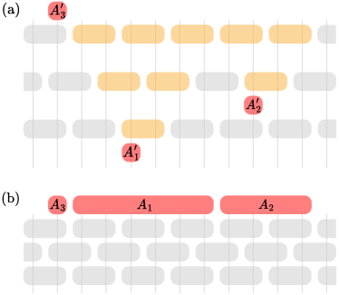
Figure 3: (a) A naïve teleportation protocol $\mathcal{W}$ and (b) the equivalent canonical-form protocol $\mathcal{W}^{\prime}$ (31). The three layers of unitary gates are the same in both protocols; the measured observables $A_{j}^{\prime}$ (in red) are modified as the unitaries in their light cone (in orange) are “pulled through” to realize $A^{\,}_{j}$ (32).

3.2 Measurement gates

The first restriction we impose relates to the projective measurements in the dilated channel $\mathcal{M}$ (16). In the literature on quantum information processing, by convention, one only considers single-qubit measurements corresponding to $Z^{\vphantom{*}}_{j}$. From a theoretical standpoint, multiqubit projective measurements are universal Nielsen (2003); Leung (2002), and can achieve teleportation acting on a trivial (product) states; as a result, no meaningful constraints can be derived in their presence. From an experimental perspective, in most quantum hardware with qubits amenable to useful quantum tasks (such as teleportation), all measurements are implemented using a combination of physical unitaries and single-qubit $Z^{\vphantom{*}}$ measurements (2.3).

Here, we restrict to the measurement of single-qubit observables $A_{j}^{\prime}$ in the naïve protocol $\mathcal{W}^{\prime}$. In the canonical-form protocol $\mathcal{W}$ (31), we allow observables $A^{\,}_{j}$ that are unitarily equivalent to single-qubit operators, i.e.,

$$A^{\vphantom{\prime}}_{j}=U\,A_{j}^{\prime}\,U^{\dagger}\,,~{}~{}$$ (32)

for generality. Since single-qubit rotations are “free” (they do not count toward the depth $T$ of $\mathcal{W}$), this restriction is equivalent to the standard one in the literature.

We now state Prop. 4, which establishes that measuring any single-qubit observable is equivalent to measuring an involutory observable (with eigenvalues $\pm 1$).

Proposition 4 (Equivalent involutory measurement).

The measurement of any nontrivial single-qubit observable $A^{\,}_{j}$ with real eigenvalues $a^{\,}_{0}>a^{\,}_{1}$ is equivalent to measurement of its involutory part $\bar{A}^{\,}_{j}$, defined to be

$$\bar{A}^{\vphantom{\dagger}}_{j} =\frac{1}{a^{\,}_{0}-a^{\,}_{1}}\sum\limits_{n=1}^{3}\,\operatorname*{tr}\limits_{j}\,\left[\,A^{\vphantom{\prime}}_{j}\,\sigma^{n}_{j}\,\right]\,\sigma^{n}_{j}$$ (33a)

$$=\left(a^{\,}_{0}-a^{\,}_{1}\right)^{-1}\,\left(2\,A^{\vphantom{\prime}}_{j}-\left(a^{\,}_{0}+a^{\,}_{1}\right)\,\mathds{1}\right)\,,~{}~{}$$ (33b)

which is unitary, Hermitian, and squares to the identity.

The proof of Prop. 4 appears in App. B. Importantly, Prop. 4 implies that all measurement channels take the simple form $\mathcal{M}^{\,}_{j}$ (2.3), with $Z^{\vphantom{*}}_{j}\to\bar{A}^{\,}_{j}$ (33). If the effective observable is given by $A^{\,}_{j}$ (32) in the canonical-form protocol $\mathcal{W}$ (31), then $\bar{A}^{\,}_{j}=U\,\bar{A}_{j}^{\prime}U^{\dagger}$, where $\bar{A}_{j}^{\prime}$ is the involutory part of the single-qubit observable $A_{j}^{\prime}$ (unitary channels preserve involutions). As a result of Prop. 4, all measurements effectively have outcomes $\pm 1$, and spectral projectors $P^{(n)}_{A}=\left(\mathds{1}+(-1)^{n}\,\bar{A}\right)/2$ (15). This also simplifies the implementation of outcome-dependent operations, and facilitates the following result.

We next state Prop. 5, which establishes that, if the outcome of a measurement channel $\mathcal{M}^{\,}_{j}$ (16) is not utilized later in the protocol $\mathcal{W}$ then, on average, $\mathcal{M}^{\,}_{j}$ either acts trivially on all logical operators or causes $\mathcal{W}$ to fail.

Proposition 5 (Necessity of feedback).

Consider the outcome-averaged Heisenberg evolution of a logical operator $\Gamma\in\mathbf{P}^{\vphantom{*}}_{*}{\rm ph}$ (2) through the measurement channel $\mathcal{M}^{\,}_{j}$ of the single-qubit observable $A^{\,}_{j}$ in the protocol $\mathcal{W}$, averaged over outcomes. If no aspect of $\mathcal{W}$ depends on the outcome of measuring $A^{\,}_{j}$, then $\mathcal{M}^{\,}_{j}$ either acts trivially on $\Gamma$ (i.e., $\Gamma\to\Gamma$), or trivializes $\Gamma$ (i.e., $\Gamma\to 0$).

The proof of Prop. 5 appears in App. C. Simply put, all projective measurements must be accompanied by at least one outcome-dependent operation to be useful to a quantum task $\mathcal{W}$ characterized by a set of logical operators. Absent feedback, a measurement either does nothing to a given logical operator $\Gamma$, or sends $\Gamma\to 0$, implying failure of $\mathcal{W}$. Hence, we may ignore any measurements in $\mathcal{W}$ without corresponding feedback.

3.3 Recovery operations

Like all useful quantum tasks, a teleportation protocol $\mathcal{W}$ outputs a state $\rho^{\,}_{T}=\lvert\Psi^{\,}_{T}\rangle\langle\Psi^{\,}_{T}\rvert$ (7), from which, e.g., one extracts expectation values of observables. Hence, $\rho^{\,}_{T}$ must be prepared and sampled many times; accordingly, when $\mathcal{W}$ involves measurements, the effective output state $\rho^{\,}_{T}$ of $\mathcal{W}$ is the one that is prepared upon averaging over outcomes. When either $\rho^{\,}_{T}$ or its logical part is pure, as with physical teleportation (see Def. 3), the above immediately implies the following Proposition.

Proposition 6 (Hybrid preparation of pure states).

Suppose that a protocol $\mathcal{W}$ involving measurements and feedback outputs the state $\rho^{\,}_{T}$ when averaged over outcomes. If the logical state $\rho^{\,}_{\rm L}=\operatorname*{tr}_{F^{c}}\left[\rho^{\,}_{T}\right]$ supported on $F\subset V$ is both pure and separable with respect to $F^{c}$, then $\mathcal{W}$ must realize $\rho^{\,}_{\rm L}$ for every sequence of measurement outcomes.

The proof of Prop. 6 appears in App. D. Note that $F^{c}$ includes all Stinespring qubits, so that $\rho^{\,}_{\rm L}$ is implicitly averaged over all outcomes. Additionally, Prop. 6 applies to protocols $\mathcal{W}$ for which $\rho^{\,}_{T}$ itself is pure. As an aside, “virtual” teleportation protocols—in which the logical state is stored in the virtual legs of a tensor network Gross and Eisert (2007); Else et al. (2012)—generally do not realize the logical states $\lvert\psi^{\,}_{n}\rangle$ on any finite subset $F\subset V$ of the physical qubits, even up to unitary operations on $F$. Instead, information is recovered from ostensibly unrelated operations Raussendorf et al. (2017); we relegate virtual teleportation to future work.

We now consider the implications for the outcome-dependent operations in $\mathcal{R}$. In general, using measurements to achieve a quantum task only outputs the desired state up to certain byproduct operators. The cost of using measurements to exceed the Lieb-Robinson bound (28) is that the state actually teleported is not $\lvert\psi\rangle$, but $\chi\,\lvert\psi\rangle$, where $\chi$ is the single-qubit byproduct operator, which is always invertible (i.e., unitary). For example, the cluster-state teleportation protocol considered in Sec. 2.4 outputs the logical state $Z^{n^{\,}_{A}}_{f}\,X^{n^{\,}_{B}}_{f}\,\lvert\psi\rangle$, rather than $\lvert\psi\rangle$ itself (on qubit $f$). Averaging over outcomes twirls the state $\rho^{\,}_{\rm L}=\lvert\psi\rangle\langle\psi\rvert$ over the Pauli matrices, so that $\rho^{\,}_{\rm L}=\mathds{1}/2$ is simply a random classical bit. The same conclusion is can be reached by considering the Heisenberg evolution of logical operators, as captured by Prop. 5.

At the same time, Prop. 6 implies that the errors introduced by measurements must be correctable for each sequence of outcomes $\boldsymbol{n}$. This is only possible if the measurement outcomes alone are sufficient to determine the byproduct operator $\chi$, and that operator is invertible, in which case one merely applies $\chi^{-1}$ to recover the logical state $\rho^{\,}_{\rm L}$ for every $\boldsymbol{n}$. This is captured by the recovery channel $\mathcal{R}$ in $\mathcal{W}$ (31), which applies physical unitaries conditioned on the states of the Stinespring qubits, which are “read only” after the corresponding measurement.

In principle, there is a broad class of dilated “recovery” channels (18) that are compatible with physical teleportation. Instead, we consider a restricted class of Clifford recovery channels, which we now define.

Definition 5.

An outcome-dependent channel $\mathcal{R}^{\,}_{\Omega}$ (18) is said to be Clifford if it can be written as

$$\mathcal{R}^{\vphantom{\dagger}}_{\Omega} =\mathds{1}\otimes\widetilde{P}^{(0)}_{\Omega}+\chi^{\vphantom{\dagger}}_{\Omega}\otimes\widetilde{P}^{(1)}_{\Omega}\,,~{}~{}$$ (34)

in the canonical-form protocol $\mathcal{W}$ (31), up to multiplication on either side by elements of the physical Clifford group $\mathbf{C}^{\vphantom{*}}_{*}{\rm ph}$, where $\chi^{\,}_{\Omega}$ is a physical Pauli string (2), $\Omega\subset\widetilde{V}$ is a subset of the Stinespring qubits, and the operators

$$\widetilde{P}^{(n)}_{\Omega}=\frac{1}{2}\Big{(}\widetilde{\mathds{1}}^{\vphantom{*}}+(-1)^{n}\,\prod\limits_{j\in\Omega}\widetilde{Z}^{\vphantom{*}}_{j}\Big{)}\,,~{}~{}$$ (35)

project onto states of $\Omega$ with $\widetilde{Z}^{\vphantom{*}}$ parity $(-1)^{n}$.

As far as we are aware, the recovery operations of all physical teleportation protocols known to the literature are Clifford in the sense of Def. 5. We also preclude outcome-dependent measurements, which are not only higher-order Clifford Gottesman and Chuang (1999) on $\mathcal{H}^{\,}_{\rm dil}$ (14), but are generally not useful to physical teleportation on their own or in combination with the Clifford recovery channels of Def. 5. Essentially, conditional measurements fail to preserve crucial properties of the logical operators (e.g., unitarity).

As an aside, we conjecture that physical teleportation protocols can be classified according to their recovery group—the set generated by the recovery operators $\chi^{\,}_{\Omega}$ for in the recovery channels $\mathcal{R}^{\,}_{\Omega}$ (34) in $\mathcal{W}$ (31) under multiplication. That group is equivalent to the set of all possible byproduct operators. Restricting to the Clifford recovery channels of Def. 5, the recovery group must be a subset of the Pauli group $\mathbf{P}^{\vphantom{*}}_{\rm ph}$. Since the phase of the logical states $\lvert\psi^{\,}_{n}\rangle$ is unimportant, we have $X^{\vphantom{*}}Z^{\vphantom{*}}\cong Z^{\vphantom{*}}X^{\vphantom{*}}$, so that the recovery group is effectively Abelian. Since $\mathbf{P}^{\vphantom{*}}_{\rm ph}$ also spans all physical operators, this is likely the simplest nontrivial recovery group that can realize. We relegate the consideration of more complicated recovery channels (and groups) to future work.

3.4 Standard teleportation protocols

We now define the “standard” teleportation protocols that we consider in the remainder. These protocols fulfill the criteria of physical teleportation and quantum state transfer (see Defs. 3 and Def. 1), as well as the properties mentioned in the preceding subsections. As far as we are aware, “standard” teleportation protocols include all physical teleportation protocols known to the literature.

Definition 6.

A standard teleportation protocol $\mathcal{W}$ is a physical teleportation protocol (see Def. 3) for which the initial state $\lvert\Psi^{\,}_{0}\rangle$ (6) is a product state and, when written in canonical form $\mathcal{W}=\mathcal{R}\,\mathcal{M}\,\mathcal{U}$ (31), (i) all measured observables $A^{\,}_{j}$ are unitarily equivalent to single-qubit operators; (ii) all recovery operations are Clifford (34) in the sense of Def. 5; (iii) no unitaries are applied to sites already measured (in the Schrödinger picture); and (iv) the task distance $L=d(I,F)>vT$ (13) exceeds the Lieb-Robinson bound (28), where $v,T$ are determined by the local unitary $\mathcal{U}$, which is compatible with Theorem 2.

We now comment on the details standard teleportation (Def. 6), compared to the more general case of physical teleportation (Def. 3). We require that $L>vT$ to ensure that $\mathcal{W}$ is a teleportation—rather than state-transfer—protocol (see Def. 1). In combinatition with the requirement that $\lvert\Psi^{\,}_{0}\rangle$ (6) be a product state, demanding $L>vT$ furnishes the locality-based analyses of Sec. 4, which also requires that $\lvert\Psi^{\,}_{0}\rangle$ be separable with respect to a biparation of the graph $G$ compatible with Lemma 11. More generally, one might restrict to states $\lvert\Psi^{\,}_{0}\rangle$ (6) that can be prepared using a FDQC $\mathcal{U}^{\,}_{0}$; however, $\mathcal{U}^{\,}_{0}$ can always be incorporated into $\mathcal{U}$ itself. The restriction to single-qubit measurements is motivated by experiment.

The remaining conditions in Def. 6 potentially preclude physical teleportation protocols. However, to the best of our knowledge, all physical teleportation protocols known to the literature obey these restrictions as well. First, the classical calculations required for teleportation cannot be arbitrary difficult; in general, one should demand that a finite number of classical bits are required to determine the outcome-dependent recovery operations. Here, we restrict to protocols that use a minimal two classical bits per qubit, captured by the Clifford recovery operations of Def. 5. We also preclude unitary operations on sites that have already been measured, as such operations (i) cannot extract further information from the state and (ii) cannot be useful to teleportation in the sense of enhancing the teleportation distance $L$ (13). This is a technical assumption that facilitates later proofs, which we generally expect can be relaxed. In Sec. 7, we comment on how assumption (ii) of Def. 6 can be relaxed.

Given a teleportation protocol $\mathcal{W}$ in canonical form (31), we define an associated resource state for $\mathcal{W}$.

Definition 7.

The resource state $\lvert\Psi^{\,}_{t}\rangle$ of a standard teleportation protocol $\mathcal{W}$ with canonical form $\mathcal{W}=\mathcal{R}\,\mathcal{M}\,\mathcal{U}$ (31) applied to the initial product state $\lvert\Psi^{\,}_{0}(\boldsymbol{\alpha},\boldsymbol{\beta})\rangle$ (6) is

$$\lvert\Psi^{\vphantom{\prime}}_{t}\rangle=\mathcal{U}\,\lvert\Psi^{\vphantom{\prime}}_{0}\rangle\,,~{}~{}$$ (36)

where $\mathcal{U}$ realizes unitary time evolution on $\mathcal{H}^{\,}_{\rm ph}$.

We note that the resource state $\lvert\Psi^{\,}_{t}\rangle$ (36) is only defined on the sites on which $\mathcal{W}$ acts. For qubits on a graph $G$ in $d>1$ dimensions, a teleportation protocol $\mathcal{W}$ acts on some path $\cal C$ connecting the initial and final logical site(s), in which case the resource state $\lvert\Psi^{\,}_{t}\rangle$ (36) refers only to the state of the qubits along the path $\mathcal{C}\subset G$.

As an aside, we do not distinguish between unitaries $\mathcal{U}$ generated by local quantum circuits versus time evolution under some local Hamiltonian. We only demand that $\mathcal{U}$ satisfies the Lieb-Robinson bound (28) of Theorem 2. The particular details of $\mathcal{U}$ are then encoded in the velocity $v$, where $v=1$ for circuits with nearest-neighbor gates.

4 Constraints on teleportation

We now derive constraints on the standard teleportation protocols $\mathcal{W}$ stipulated in Def. 6, making use of the results of Secs. 2 and 3. We assume throughout that $\mathcal{W}$ is written in canonical form (31) as detailed in Def. 4. In Sec. 4.1 we consider the action of the dilated channels on logical operators, deriving an effective form of $\mathcal{W}$ (37). We then prove numerous results for the teleportation of a single logical qubit ($k=1$), and explain how these proofs generalize to the teleportation of $k>1$ qubits in Sec. 4.4.

4.1 Action of dilated channels

Here we consider the action of single-qubit measurements (2.3) and “Clifford” recovery operations (34) on the logical operators (4) in canonical-form protocols. We first derive an effective recovery channel for the logical operators $X^{\vphantom{*}}_{{\rm L}}$ and $Z^{\vphantom{*}}_{{\rm L}}$ in Lemma 7. We then consider the combination of measurements and feedback on the logical operators in Lemma 8. Both proofs extend to any $k\geq 1$.

We now present Lemma 7, which establishes an effective recovery channel $\mathcal{R}^{\,}_{\rm eff}$ for any $\mathcal{R}$ in a canonical-form standard teleportation protocol (see Defs. 4 and 6).

Lemma 7 (Effective recovery channel).

Any standard teleportation protocol $\mathcal{W}=\mathcal{R}\,\mathcal{M}\,\mathcal{U}$ (31) that teleports a single logical qubit is equivalent to a protocol of the form

$$\mathcal{W}\cong\mathcal{W}^{\vphantom{\dagger}}_{\rm eff}=\mathcal{R}^{\vphantom{\dagger}}_{x}\,\mathcal{R}^{\vphantom{\dagger}}_{z}\,\mathcal{M}\,\mathcal{U}\,,~{}~{}$$ (37)

where $\mathcal{R}^{\,}_{x}$ ($\mathcal{R}^{\,}_{z}$) act nontrivially only on $X^{\vphantom{*}}_{{\rm L}}$ ($Z^{\vphantom{*}}_{{\rm L}}$) as

$$\mathcal{R}^{\vphantom{\dagger}}_{x} =\mathds{1}\otimes\widetilde{P}^{(0)}_{r^{\,}_{x}}+Z^{\vphantom{*}}_{{\rm L}}\otimes\widetilde{P}^{(1)}_{r^{\,}_{x}}$$ (38a)

$$\mathcal{R}^{\vphantom{\dagger}}_{z} =\mathds{1}\otimes\widetilde{P}^{(0)}_{r^{\,}_{z}}+X^{\vphantom{*}}_{{\rm L}}\otimes\widetilde{P}^{(1)}_{r^{\,}_{z}}\,,~{}~{}$$ (38b)

where $r^{\,}_{\nu}\subset\widetilde{V}$ is a subset of Stinespring qubits determined by $\mathcal{R}$ (34), the projectors correspond to outcome parities of the cluster $r^{\,}_{\nu}$ (35), $\mathcal{R}^{\,}_{x}$ and $\mathcal{R}^{\,}_{z}$ effectively commute, and $\mathcal{R}^{\,}_{\nu}=\mathds{1}$ if $\mathcal{R}$ acts trivially on $\sigma^{\nu}_{\rm L}$.

The proof of Lemma 7 appears in App. E. The Lemma establishes (i) when and how a Clifford recovery operation $\mathcal{R}^{\,}_{s}$ (34) acts nontrivially on a logical operator $\Gamma$, (ii) that the effective recovery channel $\mathcal{R}^{\,}_{\rm eff}=\mathcal{R}^{\,}_{x}\,\mathcal{R}^{\,}_{z}$ (37) is equivalent to $\mathcal{R}$ in its action on all logicals $\Gamma$ (but not other operators), and (iii) that the recovery channels for different logical operators can be written in any order, and do not mix. For $k>1$ logical qubits, the pair of channels $\mathcal{R}^{\,}_{\nu}$ (37) are replaced by $2k$ channels $\mathcal{R}^{\,}_{n,\nu}$ for $n\in[1,k]$, in any order. We stress that both $\mathcal{M}$ and $\mathcal{U}$ in $\mathcal{W}$ (37) are unaltered compared to $\mathcal{W}=\mathcal{R}\,\mathcal{M}\,\mathcal{U}$ (31).

We now state Lemma 8, which constrains the combined action of all dilated channels on logical basis operators.

Lemma 8 (Constraints on dilated channels).

Consider a standard teleportation protocol $\mathcal{W}$ in canonical form (see Defs. 4 and 6) involving the measurement of $M$ (single-qubit) observables $A^{\,}_{j}$ (32). Suppose that $\Gamma$ is a logical operator (e.g., $X^{\vphantom{*}}_{{\rm L}}$) acting on the final state $\lvert\Psi^{\,}_{T}\rangle$ (7). Then $\mathcal{W}$ fails to achieve teleportation (8) unless

$$\left[A^{\vphantom{\prime}}_{j},\,\Gamma(t^{\vphantom{\prime}}_{j})\right]=0\,,~{}~{}$$ (39)

for all observables $A^{\,}_{j}$ (32) and all logical operators $\Gamma$ evolved to the Heisenberg time $t^{\,}_{j}$ immediately prior to the measurement of $A^{\,}_{j}$. Moreover, if $\mathcal{R}$ acts nontrivially on $\Gamma$, then the measurement channel acts as

$$\Gamma(t^{\vphantom{\prime}}_{j-1})=\mathcal{M}^{\dagger}_{j}\,\Gamma(t^{\vphantom{\prime}}_{j})\,\mathcal{M}^{\vphantom{\dagger}}_{j}\cong\bar{A}^{\vphantom{\prime}}_{j}\,\Gamma(t^{\vphantom{\prime}}_{j})\,,~{}~{}$$ (40)

and trivially otherwise, where $\bar{A}^{\,}_{j}$ is the involutory part (33) of $A^{\,}_{j}$ (32) and $\cong$ becomes a genuine equality upon projecting onto the default initial Stinespring state $\lvert 0\rangle$.

The proof of Lemma 8 appears in App. F. Simply put, Lemma 8 extends Lemma 7 to the combination of a measurements and recovery operations acting on involutory logical operators $\Gamma\in\boldsymbol{\Gamma}\subset\mathbf{P}^{\vphantom{*}}_{*}{\rm ph}$. For a given $\Gamma$, this combination either acts trivially, violates the assumption that $\Gamma(t)$ remains a logical operator (i.e., involutory), or attaches the involutory part $\bar{A}^{\,}_{j}$ (33) of the measured operator $A^{\,}_{j}$ to $\Gamma(t^{\,}_{j})$, where $t^{\,}_{j}$ is the (Heisenberg) time immediately prior to the $j$th measurement. Moreover, $A^{\,}_{j}$ must commute with $\Gamma(t^{\,}_{j})$. For $\mathcal{M}^{\,}_{j}$ to act nontrivially on $\Gamma$, an odd number of recovery Paulis $\chi^{\,}_{j,k}$ conditioned on the outcome $j$ must anticommute with the operators $\Gamma(\tau^{\,}_{j,k})$, where $\tau^{\,}_{j,k}$ is the (Heisenberg) time immediately prior to the channel $\mathcal{R}^{\,}_{j,k}$. This holds for each measured observable $A^{\,}_{j}$ and all logical operators $\Gamma$.

Note that Lemma 8 holds for arbitrary (i.e., non-Clifford) $\mathcal{U}$ in the canonical-form protocol (31). The proof of Lemma 8 holds independently of any physical operations that act prior to the first measurement. Additionally, any physical unitary can be “pulled through” a measurement $\mathcal{M}^{\,}_{j}$ without affecting the result of Prop. 4, so that Lemma 8 continues to hold. Likewise, one can safely “pull through” any recovery operations $\mathcal{R}$ that act prior to some measurement (in the Schrödinger picture), to realize a canonical-form protocol (31).

Summarizing the above, the action of any canonical-form standard teleportation protocol $\mathcal{W}$ on a logical operator $\Gamma\in\boldsymbol{\Gamma}$ is constrained by Lemmas 7 and 8. The former establishes that $\mathcal{R}$ is equivalent in its action on all $\Gamma\in\boldsymbol{\Gamma}$ to the same protocol $\mathcal{W}$ with $\mathcal{R}\to\mathcal{R}^{\,}_{\rm eff}=\prod_{n=1}^{k}\,\mathcal{R}^{\,}_{n,x}\,\mathcal{R}^{\,}_{n,z}$ (37), where $\chi^{\,}_{n,\nu}$ is the other logical operator for qubit $n$ or the identity. The latter establishes that each measured observable $A^{\,}_{j}$ must commute with every logical operator $\Gamma(t^{\,}_{j})$ at the Heisenberg time $t^{\,}_{j}$ immediately prior to $\mathcal{M}^{\,}_{j}$, and that $\mathcal{M}^{\,}_{j}$ attaches $\bar{A}^{\,}_{j}$ (33) to $\Gamma(t^{\,}_{j})$ if the effective channel $\mathcal{R}^{\,}_{\Gamma}$ (38) is nontrivial (i.e., $\chi^{\,}_{\Gamma}\neq\mathds{1}$).

4.2 At least two measurements are required

We now prove that at least two measurements are needed to exceed the Lieb-Robinson bound (28), as required by Def. 6 of standard teleportation. We first prove in Prop. 9 that any physical teleportation protocol $\mathcal{W}$ (see Def. 3) involving a single measurement ($M=1$) does not exceed the bound (28): Even allowing for arbitrary outcome-dependent recovery operations, the task distance $L$ (13) realized by $\mathcal{W}$ with $M=1$ obeys the bound $L\leq vT$ (28) for $M=0$. Hence, a single measurement gives no enhancement compared to no measurements at all. In Lemma 10, we prove that two measurements (with corresponding Clifford recovery channels) are sufficient to realize $L>vT$ in standard teleportation protocols.

Proposition 9 (A single measurement is insufficient).

Consider a physical teleportation protocol $\mathcal{W}=\mathcal{R}\mathcal{M}\mathcal{U}$ (31) in canonical form (see Defs. 3 and 4), where $\mathcal{U}$ captures generic time evolution on $\mathcal{H}^{\,}_{\rm ph}$ (1) for duration $T$ and obeys the bound (28) with Lieb-Robinson velocity $v$; $\mathcal{M}$ realizes exactly one projective measurement of some (effectively) involutory observable $A$ (33); and $\mathcal{R}$ is an arbitrary recovery channel conditioned on the measurement’s outcome. If the protocol $\mathcal{W}$ teleports a single logical qubit a distance $L$ in time $T$, then $L\leq vT$.

The proof of Prop. 9 appears in App. G. Prop. 9 establishes that a single projective measurement cannot lead to a speedup compared to a protocol $\mathcal{W}^{\prime}$ with no measurements at all. Essentially, Prop. 1 is only fulfilled with $L>vT$ if the dilated channels attach distinct operators (via Lemma 8) to, e.g., the logical operators $X^{\vphantom{*}}_{{\rm L}}$ and $Z^{\vphantom{*}}_{{\rm L}}$; otherwise, $Y^{\vphantom{*}}_{{\rm L}}$ can only travel a distance $L\leq vT$.

We now consider protocols with two distinct measurements. We first present and prove Lemma 10, which establishes that a standard teleportation protocol $\mathcal{W}$ with $M=2$ can teleport a single qubit a distance $L>vT$, as well as the condition (41) that must be satisfied.

Lemma 10 (Compatible measurements).

Consider a standard teleportation protocol $\mathcal{W}$ in canonical form $\mathcal{W}=\mathcal{R}\,\mathcal{M}\,\mathcal{U}$ (see Defs. 4 and 6), where $\mathcal{U}$ realizes unitary time evolution on $\mathcal{H}^{\,}_{\rm ph}$ for duration $T$ and obeys the bound (28), $\mathcal{M}$ involves two projective measurements, and $\mathcal{R}$ consists of Clifford recovery operations (see Def. 5). If $\mathcal{W}$ teleports a logical qubit a distance $L>vT$ (13), then (i) $\mathcal{W}$ must fulfill the criteria of Lemma 8, (ii) the effective recovery channels (38) for the two logical basis operators (4) must be conditioned on different measurement outcomes, and (iii) the observables must satisfy

$$\left[A^{\,}_{1},\,A^{\,}_{2}\right]=0\,,~{}~{}$$ (41)

where $A^{\,}_{1}$ and $A^{\,}_{2}$ are the effective (involutory) operators (32) measured in the canonical-form protocol $\mathcal{W}$ (37).

The proof of Lemma 10 appears in App. H. That proof invokes many previous results, and particularly, the condition that $L>vT$. In addition to proving that $M=2$ is sufficient to realize $L>vT$ (13), the Lemma establishes a compatibility condition (41) on the canonical-form observables $A^{\,}_{1,2}$ (32). Denoting by $A_{1}^{\prime}$ and $A_{2}^{\prime}$ the single-qubit observables measured in the naïve protocol $\mathcal{W}^{\prime}$ (which need not be in canonical form), we find

$$\left[A_{1}^{\prime},\,U^{\dagger}_{12}\,A_{2}^{\prime}\,U^{\vphantom{\dagger}}_{12}\right]=0\,,~{}~{}$$ (42)

if, in the Schrödinger picture, $\mathcal{W}^{\prime}$ involves the measurement of $A_{1}^{\prime}$, followed by the physical unitary channel $U^{\,}_{12}$, followed by the measurement of $A_{2}^{\prime}$. Finally, we note that the two observables $A^{\,}_{1,2}$ (either in the naïve protocol $\mathcal{W}^{\prime}$ or in the canonical-form protocol $\mathcal{W}$) must act on different sites, or they either fail to commute or fail to realize two distinct physical observables, so that Prop. 9 applies.

The compatibility condition (41) makes sense when one considers the information that can be extracted from the resource state $\lvert\Psi_{t}\rangle$ (36). Suppose that one measures $Z^{\vphantom{*}}_{j}$ on site $j$. Measuring $Z^{\vphantom{*}}_{j}$ again is gives the same outcome, while measuring $X^{\vphantom{*}}_{j}$ or $Y^{\vphantom{*}}_{j}$ gives a random outcome; in either case, no new information can be extracted. In the naïve protocol, the single-qubit measurements only extract information from the resource state if they act on distinct sites or if there are intervening multiqubit unitaries. For the canonical-form observables (32), one expects that at most $n$ independent outcomes can be extracted from $n$ qubits via measurements, provided that the $n$ observables mutually commute.

However, it remains to understand how a pair of compatible measurements can be useful to teleportation, as well as the extent of that utility in terms of exceeding the measurement-free Lieb-Robinson bound (28). We now present Lemma 11, which establishes the maximum enhancement to the teleportation distance $L=d(i,f)$ (13) that a pair of compatible measurements (41) can realize, using the fact that $\mathcal{U}$ obeys the bound (28).

Lemma 11 (Speedup from two measurements).

Consider a standard teleportation protocol $\mathcal{W}$ (see Def. 6) in canonical form $\mathcal{W}=\mathcal{R}\,\mathcal{M}\,\mathcal{U}$ (37), where $\mathcal{U}$ is a local unitary (e.g., an FDQC) that obeys the bound (28) with Lieb-Robinson velocity $v$ and total duration (or depth) $T$, $\mathcal{M}$ involves the measurement of two compatible, involutory observables $A^{\,}_{1}\neq A^{\,}_{2}$, and $\mathcal{R}$ involves outcome-dependent operations that are useful in the sense of Lemma 10. Then the task distance $L=d(i,f)$ (13) obeys the bound

$$L\leq v(3T-2)-2v\,\max_{\nu}\tau^{\,}_{\nu}\,,~{}~{}$$ (43)

where $\tau^{\,}_{\nu}$ is the total duration of time evolution following the measurement of $A_{\nu}^{\prime}$ in the naïve protocol $\mathcal{W}^{\prime}$ (in the Schrödinger picture), and $T\geq 2$.

The proof of Lemma 11 appears in App. I, and relies on the fact that the light cones of both measured observables must intersect with that of the final-state logical operator $\sigma^{\nu}_{f}$ (at some site $\ell\approx i+2L/3$). The intuition is that measurements “reflect” (or “link up”) light cones Friedman et al. (2022a), leading to a threefold enhancement to $v$ in the $M=2$ bound (43) compared to $L\leq vT$ (28) for $M<2$.

4.3 Additional measurement regions

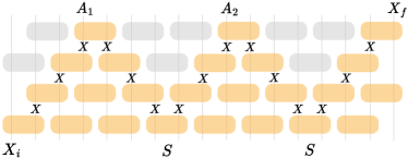
Figure 4: The light cones of measured observables in canonical form are illustrated in a FDQC. The light cones of the logical operator and the measured observables $A^{\,}_{j}$ attached thereto via Lemma 8 must intersect for teleportation to succeed.

We next turn to standard teleportation protocols that achieve a task distance $L>3vT$ (13), which exceeds the bound (43) of Lemma 11 for $M=2$. Theorem 3 Friedman et al. (2022a) suggests that this is possible if one uses additional measurements and accompanying feedback to link up the light cones of the additional measured observables attached to the logical operators, as depicted in Fig. 4.

As a starting point, consider a protocol $\mathcal{W}=\mathcal{W}^{\,}_{m}\cdots\mathcal{W}^{\,}_{1}$ in which $m$ teleportation protocols $\mathcal{W}^{\,}_{s}$ are applied in series. Each protocol $\mathcal{W}^{\,}_{s}$ satisfies $L^{\,}_{s}=d(i_{s},f_{s})\leq v(3\,T^{\,}_{s}-2)$ (43), where $f_{s}=i_{s+1}$ is the initial site of the subsequent protocol, so that the total distance (13) is

$$L =d(i^{\,}_{1},f^{\,}_{m})=\sum\limits_{s=1}^{m}L^{\vphantom{\prime}}_{s}v\,\sum\limits_{s=1}^{m}(3\,T^{\vphantom{\prime}}_{s}-2)$$

$$\leq v(3\,T-2\,m)<3\,v\,T\,,~{}~{}$$ (44)

where $T=\sum_{s}T^{\,}_{s}$ is the total depth. Unsurprisingly, applying protocols in series obeys the same bound (43).

However, an improvement can be realized by applying the protocols in parallel. Most of the channels in the protocol $\mathcal{W}^{\,}_{s}$ do not overlap with those of $\mathcal{W}^{\,}_{s-1}$. For convenience, suppose each protocol $\mathcal{W}^{\,}_{s}$ has the same depth $T^{\,}_{s}=T^{\prime}$. As explained following Lemma 11, each protocol $\mathcal{W}^{\,}_{s}$ uses $M^{\,}_{s}=2$ measurements to link a unitary “staircase” region of size $\ell^{\,}_{s,{\rm uni}}\leq vT^{\prime}$ and another measurement-assisted “light-cone” region of size $\ell^{\,}_{s,{\rm meas}}\leq 2v(T^{\prime}-1)$.

Crucially, this perspective elucidates how to achieve parallelization. The unitaries that act in the light-cone regions can all be applied in parallel in time $T^{\prime}$. The unitaries in each staircase region must be applied after all light-cone unitaries, for an additional unitary depth of $T^{\prime}$, so that the final site $f_{s}$ of protocol $s$ is the initial site $i_{s+1}$ of protocol $s+1$. After time $2T^{\prime}$, all measurements and outcome-dependent operations are applied. Noting that the total unitary depth is $T=2T^{\prime}$, the task distance $L$ (13) for the parallelized protocol obeys

$$L^{\vphantom{\prime}}_{\rm par} \leq\frac{3}{4}v\,M\left(T-\frac{4}{3}\right)\,,~{}~{}$$ (45)

which exceeds the $M=2$ bound (43) when $M>4$.

However, it is possible to exceed the bound (45) by constructing fully parallel protocols. In particular, by omitting the staircase segments of each protocol $\mathcal{W}^{\,}_{s}$ except $\mathcal{W}^{\,}_{1}$, the total depth can be cut in half compared to the parallelized case. As a result, the upper bound (45) is modified by sending $T\to 2T$ and subtracting $(m-1)vT$. The resulting bound for a generic standard teleportation protocol with $M>1$ is captured by Lemma 12.

Lemma 12 (Maximum speedup for $M$ measurements).

The distance $L=d(i,f)$ (13) that a standard teleportation protocol $\mathcal{W}=\mathcal{R}\,\mathcal{M}\,\mathcal{U}$ (where $\mathcal{U}$ has depth $T$ and speed limit $v$) can transfer a single logical state $\lvert\psi\rangle$ using $M$ measurements and accompanying feedback obeys

$$L\leq vT+2v\left\lfloor\frac{M}{2}\right\rfloor\left(T-1\right)\,,~{}~{}$$ (46)

where the $vT$ term captures the measurement-free distance and the second term captures the maximum enhancement due $M$ measurements. We must have $T\geq 2$, as in Lemma 11, and the separation $\ell$ between pairs of measurements obeys $\ell\leq 2v(T-1)$.

The proof of Lemma 12 appears in App. J. The bound (46) is saturated by parallel protocols in which $m=M/2$ pairs of measurements are spaced by a distance $\ell=2v(T-1)$ to daisy chain $m=\lfloor M/2\rfloor$ light-cone regions of size $\ell$ and a single staircase region of size $\ell^{\,}_{0}\leq vT$. Note that Eq. 46 saturates the $k=1$ bound (30) Friedman et al. (2022a), up to $\mathsf{O}\left(1\right)$ offsets, while the teleportation bound (29) of Theorem 3 with $k=1$ is loose by a factor of two compared to the $k=1$ bound (46), as conjectured in Ref. 36.

At this point, we note that the “measurement regions” discussed in Ref. 36 are only unambiguously defined for optimal protocols. In that case, each pair of (adjacent) measurements used to daisy chain regions in the proof of Lemma 12 (see App. J) defines a distinct measurement region (the support of the pair of operators). There are $M=\lfloor M/2\rfloor$ such regions in total, where the $s$th region has size $v+1\leq\ell^{\,}_{s}\leq 2v(T-1)$. However, we note that (i) the bounds herein are all phrased in terms of the number of measurement outcomes and (ii) an unambiguous delineation of measurement regions can be identified even in suboptimal protocols by considering string order, as we establish in Sec. 5.

4.4 Multiqubit teleportation

We now generalize the foregoing results to standard teleportation protocols $\mathcal{W}$ (see Def. 6) that transfer $k\geq 1$ logical qubits. We first note that the various results of Sec. 4.1 apply directly to protocols with $k>1$ as stated. Next, the proofs of Prop. 9 and Lemma 10 include proofs for $k>1$ logical qubits. Essentially, $M\geq 2k$ are required, or else at least one logical qubit is teleported using a single outcome, which is impossible; moreover, all measured observables must commute. Using these results, we now state the most general bound for standard teleportation protocols, captured by Theorem 13.

Theorem 13 (Standard teleportation bound).

Consider a standard teleportation protocol $\mathcal{W}=\mathcal{R}\,\mathcal{M}\,\mathcal{U}$ written in canonical form (31), where $\mathcal{U}$ realizes unitary time evolution for duration $T$ with Lieb-Robinson velocity $v$ and $\mathcal{M}$ consists of $M>1$ projective measurements. Then $\mathcal{W}$ can teleport $k$ logical qubits a distance (13)

$$L\leq vT+2\,v\left\lfloor\frac{M}{2k}\right\rfloor\left(T-1\right)\,,~{}~{}$$ (47)

where $\lfloor\cdot\rfloor$ is the floor function, and $T$ obeys

$$T\geq 1+k/v\,,~{}~{}$$ (48)

where all measured observables $A^{\,}_{j}$ (32) commute with one another and with all final-state logical operators (7).

The proof of Theorem 13 appears in App. K. The bounds (47) and (48) follow from identifying the optimal protocol described in the Theorem, which is further constrained in the proof in App. K. Essentially, each of the $k$ logical qubits can be treated individually, and all previous results apply, giving the bound (47). The depth constraint (48) follows from recognizing that there must be ample spacing between equivalent measurements to accommodate all $2k$ measurements required per region.

The perspective is that a single region of size $\ell^{\,}_{0}\leq vT$ can be daisy chained with $m$ regions of size $2k\leq\ell\leq 2v(T-1)$ using measurements of $2k$ sites. In the optimal case, the measurements are made on $2k$ consecutive sites, where the sites $2n-1$ and $2n$ correspond to the $n$th logical qubit. In this scenario, the optimal spacings of initial and final sites are given by $i_{n}=i_{1}+2(n-1)$ and $f_{n}=f_{1}+2(n-1)$, respectively.

Finally, we remark that the teleportation bound (47) is tighter than corresponding bound (29) of Theorem 3 and Ref. 36. Essentially, Eq. 29 is loose by a factor of two in the context of standard teleportation protocols, as initially conjectured in Ref. 36. While, in principle, it is possible that nonstandard teleportation protocols could exceed the teleportation bound (47)—and instead obey Eq. 29—we note that (i) both bounds have the same asymptotic scaling in terms of $L$, $M$, and $T$, which makes them equivalent in the context of such locality bounds, and (ii) as far as we are aware, the types of channels that we have eschewed in our analysis of optimal protocols in App. K—such as conditional measurements and non-Pauli recovery operations—cannot lead to violations of the standard bound (47). Hence, we expect that Eq. 47 optimally bounds all physical teleportation protocols.

4.5 Suboptimal measurements

Before moving on to the main results in Sec. 5, we briefly discuss suboptimal measurements. There are a number of ways in which a standard teleportation protocol $\mathcal{W}$ (see Def. 6) can fail to be optimal in the sense of saturating the teleportation bound (47). Of these, only protocols that involve more measurements than are necessary for a given teleportation distance $L$ (13) have the potential to complicate the main results in Sec. 5.

However, the requirement in Def. 6 that no unitaries be applied to qubits that have already been measured (in the Schrödinger picture) avoids this complication. The analysis of Sec. 5 requires that all of the measurements that are useful to teleportation commute, and that the rest can be considered part of the preparation of the resource state (e.g., in the sense that there exists an equivalent protocol in which these measurements are replaced by unitaries). As we establish below, in Corollary 14 of Lemma 8, the aforementioned criterion of Def. 6 ensures that all “useful” measured observables commute with each other and with all logical operators, and that all other measurements can be omitted without consequence.

Corollary 14 (Necessary measurements commute).

The measurements that are necessary for teleportation correspond to observables that (i) commute with one another and (ii) have no support on the final logical sites $f\in F$. The remaining observables are (i) applied to sites that were already usefully measured, (ii) anticommute with that useful measurement and thus have a random outcome, (iii) are not attached to any logical operator via Lemma 8, and (iv) may simply be omitted from $\mathcal{W}$.

The proof of Corollary 14 is straightforward and appears in App. L. As we note in Sec. 3.4 below Def. 6, we expect that the result above holds generically, even if the requirement that no unitaries are applied to previously measured sites (in the Schrödinger picture) is relaxed.

5 The resource state is an SPT

We now derive the main result: Standard teleportation protocols involve preparing an SPT resource state $\lvert\Psi_{t}\rangle=\mathcal{U}\,\lvert\Psi_{0}\rangle$ (36) protected by a $\mathbb{Z}^{\,}_{2}\times\mathbb{Z}^{\,}_{2}$ symmetry, measuring the corresponding string order parameters, and applying outcome-dependent Pauli gates. We briefly review SPTs in Sec. 5.1 before proving that the resource state $\lvert\Psi_{t}\rangle$ for $k=1$ teleportation has $\mathbb{Z}^{\,}_{2}\times\mathbb{Z}^{\,}_{2}$ string order. We then extend this result to $k>1$ in Sec. 5.3, where the protecting symmetry consists of (at least) $k$ copies of $\mathbb{Z}^{\,}_{2}\times\mathbb{Z}^{\,}_{2}$, each corresponding to pairs of sublattices.

5.1 Overview of SPTs

We begin with a brief summary of 1D SPT phases and their salient features. For the SPTs of interest, the “protecting symmetry” corresponds to a group $\mathcal{G}$, whose generators $g\in\mathcal{G}$ have an on-site representation

$$U(g)=\prod\limits_{j=1}^{N}\,u_{j}(g)\,,~{}~{}$$ (49)

where the $u_{j}(g)$ is a unitary representation of $g$ on site $j$.

A 1D SPT phase is captured by a state $\lvert\Phi\rangle$ that is symmetric under $U(g)$ (49). Because the chain may be open or closed, the definition of a symmetric state must be independent of boundary conditions. We denote by $\mathcal{I}\subseteq[1,N]$ a subinterval of the chain, and define $U_{\mathcal{I}}(g)$ as the restriction of $U(g)$ (49) to the interval $\mathcal{I}$. Then $\lvert\Psi\rangle$ is symmetric under $U(g)$ (49) if, for every interval $\mathcal{I}$ with $\lvert\mathcal{I}\rvert\gg\xi$ (where $\xi$ is the correlation length of $\lvert\Psi\rangle$), there exist “endpoint operators” $V_{L}(g)$ and $V_{R}(g)$ localized to the left and right boundaries of $\mathcal{I}$, respectively, such that

$$V_{L}(g)\,U_{\mathcal{I}}(g)\,V_{R}(g)\,\lvert\Psi\rangle=\lvert\Psi\rangle\,,~{}~{}$$ (50)

meaning that applying the on-site symmetry operators $u_{j}(g)$ in $U(g)$ (49) to some subregion $\mathcal{I}$ only affects the symmetric state $\lvert\Psi\rangle$ near the boundaries of $\mathcal{I}$. Eq. (50) can be shown rigorously using matrix product states Pérez-García et al. (2008).

The operators $V_{L}(g)\,U_{\mathcal{I}}(g)\,V_{R}(g)$ in Eq. 50 are known as string order parameters Pollmann and Turner (2012). More generally, a string order parameter is any operator consisting of an on-site representation $u_{j}(g)$ (49) of $g\in\mathcal{G}$ in an interval $\mathcal{I}$ decorated by charged operators $V$ at the endpoints Pollmann and Turner (2012). Here, we can always choose endpoints such that the string order is perfect, meaning it has expectation value one. While the operators $u_{j}(g)$ in $U(g)$ (49) realize a linear representation of $g\in\mathcal{G}$, the endpoint operators $V_{L/R}(g)$ only realize a projective representation of $g\in\mathcal{G}$, i.e.,

$$V_{L}(g)\,V_{L}(h) =\omega(g,h)\,V_{L}(gh)$$ (51a)

$$V_{R}(g)\,V_{R}(h) =\omega^{-1}(g,h)\,V_{L}(gh)\,,~{}~{}$$ (51b)

for all $g,h\in\mathcal{G}$, where $\omega(g,h)\in\mathsf{U}\left(1\right)$ is a complex phase. This phenomenon is known as symmetry fractionalization, and is the basis for classifying SPT phases in 1D Chen et al. (2011); Schuch et al. (2011); Pollmann et al. (2010).

For the finite Abelian groups $\mathcal{G}$ relevant herein, it is useful to define an additional complex phase $\Omega(g,h)$ via

$$V_{L}(g)\,V_{L}(h)=\Omega(g,h)\,V_{L}(h)\,V_{L}(g)\,,~{}~{}$$ (52)

where one can check that $\Omega(g,h)=\omega(g,h)\,\omega^{-1}(h,g)$. We now define nontrivial string order using the phases $\Omega$.

Definition 8.

A state $\lvert\Psi\rangle$ has nontrivial string order with respect to an (Abelian) symmetry group $\mathcal{G}$ if, for every subinterval $\mathcal{I}\subseteq[1,N]$, there exist endpoint operators $V_{L}(g)$ and $V_{R}(g)$ localized to the boundary of $\mathcal{I}$ satisfying $\Omega(g,h)\neq 1$ (52) for some choice of $g,h\in\mathcal{G}$, along with

$$\left\langle\Psi\middle|\,V_{L}(g)\,U_{\mathcal{I}}(g)\,V_{R}(g)\,\middle|\Psi\right\rangle=1\,,~{}~{}$$ (53)

where $U_{\mathcal{I}}(g)$ is the restriction of $U(g)$ (49) to $\mathcal{I}$.

The fact that $\Omega(g,h)\neq 1$ for some $g,h\in\mathcal{G}$ is necessary and sufficient for the projective representation to belong to a nontrivial class is shown in Berkovich and Zhmud (1998). One can show that nontrivial string order (53) implies that (i) any gapped Hamiltonian with symmetry group $\mathcal{G}$ and ground state $\lvert\Psi\rangle$ has zero-energy edge modes Pollmann et al. (2010) and (ii) the state $\lvert\psi\rangle$ cannot be mapped to a product state via a FDQC consisting of local gates that respect the symmetry Huang and Chen (2015). Accordingly, nontrivial string order (53) of $\lvert\Psi\rangle$ is often regarded as synonymous with nontrivial SPT order of $\lvert\Psi\rangle$ (or the parent Hamiltonian). However, since SPT order delineates a phase of matter, it is only well defined in the thermodynamic limit Zeng and Wen (2015). Hence, establishing SPT order more carefully requires considering a family of states $\lvert\Psi\rangle$ defined on chains of increasing length, each of which possesses nontrivial string order in the sense of Def. 8.

5.2 Single-qubit case: $\mathbb{Z}^{\,}_{2}\times\mathbb{Z}^{\,}_{2}$

We first prove that standard teleportation protocols $\mathcal{W}$ that teleport a single logical qubit ($k=1$), when written in canonical form (31), correspond to preparing an SPT resource state $\lvert\Psi^{\,}_{t}\rangle$ (36), measuring its string order parameters, and applying Pauli recovery gates to the final site $f$. In particular, the nontrivial string order of $\lvert\Psi^{\,}_{t}\rangle$ (36) is with respect to the discrete Abelian symmetry $\mathcal{G}=\mathbb{Z}^{\,}_{2}\times\mathbb{Z}^{\,}_{2}$. The endpoint operators satisfy the Pauli algebra generated by $X^{\vphantom{*}}$ and $Z^{\vphantom{*}}$, which realize a projective representation of $\mathcal{G}$. As a first step toward proving that $\lvert\Psi^{\,}_{t}\rangle$ (36) has nontrivial string order in the sense of Def. 8, we first present Lemma 15, establishing the existence of order parameters (53) when $\mathcal{I}$ is the full chain.

Lemma 15 (End-to-end string order parameter).

Suppose that the standard teleportation protocol $\mathcal{W}$ teleports $k=1$ logical qubit from $i$ to $f$ and has canonical form $\mathcal{W}=\mathcal{R}\,\mathcal{M}\,\mathcal{U}$ (31). Then the resource state $\lvert\Psi^{\,}_{t}\rangle$ (36) has string order characterized by, e.g., the order parameters

$$\left\langle\Psi^{\vphantom{\prime}}_{t}\middle|\,\mathcal{U}\,X^{\vphantom{*}}_{i}\,\mathcal{U}^{\dagger}\,\bar{A}^{\vphantom{\prime}}_{x}\,X^{\vphantom{*}}_{f}\,\middle|\Psi^{\vphantom{\prime}}_{t}\right\rangle =1$$ (54a)

$$\left\langle\Psi^{\vphantom{\prime}}_{t}\middle|\,\mathcal{U}\,Z^{\vphantom{*}}_{i}\,\mathcal{U}^{\dagger}\,\bar{A}^{\vphantom{\prime}}_{z}\,Z^{\vphantom{*}}_{f}\,\middle|\Psi^{\vphantom{\prime}}_{t}\right\rangle =1\,,~{}~{}$$ (54b)

where the bulk operators are given by

$$\bar{A}^{\vphantom{\prime}}_{\nu}\equiv\bar{A}_{1}^{\lambda^{\,}_{1,\nu}}\cdots\bar{A}_{M}^{\lambda^{\,}_{M,\nu}}\,,~{}~{}$$ (55)

i.e., the product of the involutory parts (33) of all necessary measured observables $\bar{A}^{\,}_{j}$ (see Cor. 14) attached to $\sigma^{\nu}_{f}$ by Lemma 8. Hence, the string order parameters (54) commute in the bulk region $(i+vT,f)$, i.e.,

$$\left[\bar{A}^{\vphantom{\prime}}_{x},\,\bar{A}^{\vphantom{\prime}}_{z}\right]=0\,,~{}~{}$$ (56)

while the endpoint operators $\mathcal{U}\,\sigma^{\nu}_{i}\,\mathcal{U}^{\dagger}$ and $\sigma^{\nu}_{f}$ anticommute for different $\nu=x,z$, as required by Def. 8.

The proof of Lemma 15 appears in App. M, and follows straightforwardly from previous results. The end-to-end string order parameters are depicted graphically in Fig. 5(a). The operators above $\mathcal{U}$ represent the two string order parameters (54) acting on the resource state $\lvert\Psi^{\,}_{t}\rangle$ (36), with the anticommuting endpoint operators color coded. In the Heisenberg picture, the order parameters evolve under $\mathcal{U}$ into the stabilizers $\mathsf{S}^{\,}_{x,z}\in\operatorname*{stab}\left(\lvert\Psi^{\,}_{0}\rangle\right)$ at the bottom of Fig. 5(a), which have expectation value one (50) acting on the initial state $\lvert\Psi^{\,}_{0}\rangle$ (6).

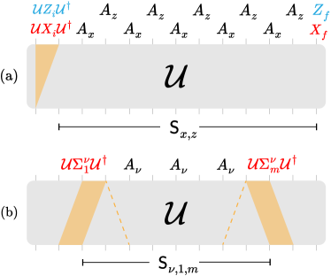
Figure 5: The construction of $\mathbb{Z}^{\,}_{2}\times\mathbb{Z}^{\,}_{2}$ string order parameters (a) on the endpoints and (b) in the bulk, where the colored operators represent the anticommuting endpoints.

However, in general, a state is only said to have string order (53) if a similar relation holds for many choices of endpoints. As it turns out, the string order parameters (54) in Lemma 15, with right endpoint $f$ and left endpoint in $[i,i+vT]$, are not the only valid choice for the resource state $\lvert\Psi^{\,}_{t}\rangle$ (36). In Lemma 16, we prove that a set of valid string order parameters (53) corresponding to various subintervals $\mathcal{I}\subset[i,f]$ can be identified.

Lemma 16 ($\mathbb{Z}^{\,}_{2}\times\mathbb{Z}^{\,}_{2}$ string order).

In addition to the end-to-end string order parameter (54) of Lemma 15, the resource state $\lvert\Psi^{\,}_{t}\rangle$ (36) exhibits nontrivial string order (see Def. 8) captured by the order parameters

$$\mathcal{S}^{\vphantom{\prime}}_{\nu,a,b}=\left(\mathcal{U}\,\Sigma^{\nu}_{a}\,\mathcal{U}^{\dagger}\right)\,\bar{A}^{\vphantom{\prime}}_{\nu,a+1}\cdots\bar{A}^{\vphantom{\prime}}_{\nu,b}\,\left(\mathcal{U}\,\Sigma^{\nu}_{b}\,\mathcal{U}^{\dagger}\right)\,,~{}~{}$$ (57)

where the left and right endpoints are given by

$$\mathcal{U}\,\sigma^{\nu}_{i}\,\mathcal{U}^{\dagger}\to\mathcal{U}\,\Sigma^{\nu}_{a}\,\mathcal{U}^{\dagger}~{}~{},~{}~{}\sigma^{\nu}_{f}\to\mathcal{U}\Sigma^{\nu}_{b}\,\mathcal{U}^{\dagger}\,,~{}~{}$$ (58)

compared to Eq. 54, where the new endpoint operator is

$$\Sigma^{\nu}_{s} =\sigma^{\nu}_{i}\,\mathcal{U}^{\dagger}\,\bar{A}^{\vphantom{\prime}}_{\nu,1}\cdots\bar{A}^{\vphantom{\prime}}_{\nu,s}\,\mathcal{U}=\Sigma^{\nu}_{s-1}\,\mathcal{U}^{\dagger}\,\bar{A}^{\vphantom{\prime}}_{\nu,s}\,\mathcal{U}\,,~{}~{}$$ (59)

where $\Sigma^{\nu}_{0}=\sigma^{\nu}_{i}$ and $\left\{\Sigma^{x}_{s},\,\Sigma^{z}_{s}\right\}=0$, as required. The $m$ operators $\bar{A}^{\,}_{s}$ correspond to products of the measured observables $\bar{A}^{\,}_{j}$ (33) in disjoint regions labeled $s$, such that $\mathcal{U}^{\dagger}\,\bar{A}^{\,}_{s+1}\,\mathcal{U}$ has no overlap with $\Sigma^{\nu}_{s}$ and $\Sigma^{\nu}_{s}$ acts to the right of $\Sigma^{\nu}_{s-1}$ and to the left of $\Sigma^{\nu}_{s+1}$.

Since, for all $a<b\in[1,m]$, $\lvert\Psi^{\,}_{t}\rangle$ (36) satisfies

$$\left\langle\Psi^{\vphantom{\prime}}_{t}\middle|\mathcal{S}^{\vphantom{\prime}}_{\nu,a,b}\middle|\Psi^{\vphantom{\prime}}_{t}\right\rangle=1\,,~{}~{}$$ (60)

the resource state has nontrivial string order (see Def. 8).

The proof of Lemma 16 appears in App. N. The Lemma shows that the resource state $\lvert\Psi^{\,}_{t}\rangle$ (36) has nontrivial string order captured by a set of order parameters (57) corresponding to intervals $\mathcal{I}\subseteq[i,f]$. Valid endpoints are labelled $s=[0,m+1]$, where $s=0$ corresponds to $j\approx i+vT$, $s=m+1$ to $j=f$, and all others to the $m$ nonoverlapping “measurement regions.”

The string order parameters (57) are illustrated in Fig. 5(b). The operator $\Sigma^{\nu}_{1}$ is guaranteed to have no overlap in support with $\mathcal{U}^{\dagger}\bar{A}^{\,}_{\nu,2}$—the observable immediately to the right of the left endpoint operator in Fig. 5(b)—by Lemma 16. This can be ensured by multiplying the “naïve” choice of $\Sigma^{\nu}_{1}$ by an initial-state stabilizer $\mathsf{S}^{\,}_{\nu,1}$ to remove any support in triangle defined by the parallelogram and dashed line. The same holds for the right endpoint operator. We also point out that $\Sigma^{\nu}_{1}$ has no overlap with $\sigma^{\nu}_{i}$, and that this extends to any choice of interval $\mathcal{I}=[a,b]$, where the endpoint operators of the corresponding string order parameter $\mathcal{S}^{\,}_{\nu,a,b}$ (57) have no overlap with those of $\mathcal{S}^{\,}_{\nu,a\pm 1,b}$ nor $\mathcal{S}^{\,}_{\nu,a,b\pm 1}$ by Lemma 16.

The string order parameters (57) indicate that $\lvert\Psi^{\,}_{t}\rangle$ (36) is symmetric (50) with respect to a group $\mathcal{G}=\mathbb{Z}^{\,}_{2}\times\mathbb{Z}^{\,}_{2}$, which is projectively represented by the Pauli matrices $\{\mathds{1},X^{\vphantom{*}},Y^{\vphantom{*}},Z^{\vphantom{*}}\}$, so that $\Omega(x,z)=-1$ (52). In the bulk, $\mathcal{G}$ has a linear (unitary) representation

$$U_{\mathcal{I}}(\nu)=\prod\limits_{s\in\mathcal{I}}\,\bar{A}^{\vphantom{\prime}}_{\nu,s}\,,~{}~{}$$ (61)

where $\nu\in\{x,z\}$ and $\left[U_{\mathcal{I}}(x),\,U_{\mathcal{I}}(z)\right]=0$ by Cor. 14, which is on site for a sufficiently large unit cell.

However, for nontrivial string order (60) to imply an SPT, one must show that the string order corresponds to a phase of matter. This requires that one can extend Eqs. 57 and 60 to the thermodynamic limit (where $\lvert\mathcal{I}\rvert\to\infty$), which we establish in the following Corollary.

Corollary 17 (Embedding the resource state).

The resource state $\lvert\Psi^{\,}_{t}\rangle$ (36) can be embedded in a thermodynamically large (i.e., infinite) chain, and the string order (60) extended to arbitrarily large intervals by implementing the truncation procedure of Lemma 16 in reverse.

Corollary 17 follows from Lemma 16 and its proof in App. N. The Corollary establishes that one can use the resource state $\lvert\Psi^{\,}_{t}\rangle$ (36) to define a family of states of unbounded length, each of which has perfect string order, meaning that the string order survives into the thermodynamic limit. This also establishes that $\lvert\Psi^{\,}_{t}\rangle$ (36) cannot be prepared in finite time $t\ll d(i,f)$ under local unitary time evolution (with $v=\mathsf{O}\left(1\right)$ finite) that respects the symmetry $\mathcal{G}=\mathbb{Z}^{\,}_{2}\times\mathbb{Z}^{\,}_{2}$ Huang and Chen (2015). Thus, the resource state (36) for any $k=1$ standard teleportation protocol $\mathcal{W}$ belongs to a nontrivial SPT phase indicated by $\mathbb{Z}^{\,}_{2}\times\mathbb{Z}^{\,}_{2}$ string order, where the measured operators $A_{j}$ used to determine $\mathcal{R}_{x/z}$ (38) are those that make up the bulk of the $x/z$ string order parameters (57).

5.3 Multiqubit case: $\mathbb{Z}_{2}^{2k}$

We now show that the results of Sec. 5.2 for a single logical qubit extend straightforwardly to the standard teleportation of $k>1$ logical qubits. This result is established by Theorem 18, which we state and prove below.

Theorem 18 (Standard teleportation implies SPT order).

Consider a protocol with canonical form $\mathcal{W}=\mathcal{R}\,\mathcal{M}\,\mathcal{U}$ (31) that achieves standard teleportation of $k\geq 1$ qubits (see Def. 6). Omitting any unnecessary measurements from $\mathcal{M}$ (see Cor. 14), we identify $m$ measurement regions—where $\bar{A}^{\,}_{n,\nu,s}$ is a product of all measured observables $\bar{A}^{\,}_{j}$ (33) in region $s$ attached to $\sigma^{\nu}_{f_{n}}$ (40)—such that $\bar{A}^{\,}_{n,\nu,s+1}$ has no overlap with the endpoint operator

$$\Sigma^{\nu}_{n,s} =\sigma^{\nu}_{i_{n}}\,\mathcal{U}^{\dagger}\,\bar{A}^{\vphantom{\prime}}_{n,\nu,1}\cdots\bar{A}^{\vphantom{\prime}}_{n,\nu,s}\,\mathcal{U}$$

$$=\Sigma^{\nu}_{n,s-1}\,\mathcal{U}^{\dagger}\,\bar{A}^{\vphantom{\prime}}_{n,\nu,s}\,\mathcal{U}\,,~{}~{}$$ (62)

where $\Sigma^{\nu}_{n,0}=\sigma^{\nu}_{i_{n}}$ and $\Sigma^{\nu}_{n,m+1}=\mathcal{U}^{\dagger}\,\sigma^{\nu}_{f_{n}}\,\mathcal{U}$. Then, for all $n\in[1,k]$, $\nu=x,y,z$, and $a<b\in[1,m]$, the operator

$$\mathcal{S}^{n,\nu}_{a,b}\equiv\mathcal{U}\,\Sigma^{\nu}_{n,a}\,\mathcal{U}^{\dagger}\,\bar{A}^{\vphantom{\prime}}_{n,\nu,a+1}\cdots\bar{A}^{\vphantom{\prime}}_{n,\nu,b}\,\mathcal{U}\,\Sigma^{\nu}_{n,b}\,\mathcal{U}^{\dagger}\,,$$ (63)

with anticommuting endpoint operators $\Sigma^{\nu}_{n,s}$ (62) satisfies

$$\left\langle*\middle|\Psi^{\vphantom{\prime}}_{t}\middle|\,\mathcal{S}^{n,\nu}_{a,b}\,\right\rangle{\Psi^{\vphantom{\prime}}_{t}}=1\,,~{}~{}$$ (64)

for the resource state $\lvert\Psi^{\,}_{t}\rangle$ (36), indicating nontrivial string order (see Def. 8) with respect to the symmetry

$$\mathcal{G}_{k}=\left(\mathbb{Z}^{\vphantom{\prime}}_{2}\times\mathbb{Z}^{\vphantom{\prime}}_{2}\right)^{k}=\mathbb{Z}^{2k}_{2}\,,~{}~{}$$ (65)

so that $\mathcal{U}$ prepares a resource state $\lvert\Psi^{\,}_{t}\rangle$ (36) with nontrivial SPT order, $\mathcal{M}$ measures its end-to-end (54) string order parameters $\mathcal{S}^{n,\nu}_{0,m+1}$ (63), and $\mathcal{R}$ corrects the errors $\chi$, which belong to a projective representation of $\mathcal{G}_{k}$ (65).

Proof.

The case for $k=1$ is proven in Lemmas 15 and 16. By definition, the logical operators for different logical qubits commute; by Cor. 14, all necessary measured observables commute for any $k$, while all other measurements have been omitted without affecting $\mathcal{W}$. Thus, Lemmas 15 and 16 hold for each logical qubit individually (i.e., independently): The preceding arguments guarantee that the string order parameters (63) for distinct logical qubits locally commute. Moreover, Cor. 17 extends to $k>1$ without caveat. As a result, $\lvert\Psi^{\,}_{t}\rangle$ (36) belongs to a nontrivial SPT phase with $\mathbb{Z}^{2k}_{2}$ string order. ∎

Theorem 18 is the main result of this paper. In the optimal case, the $M=2km$ measurements are applied to the $2k$ sublattices of the chain at the endpoints of each valid subinterval $\mathcal{I}$ described in Sec. 5.1. The same resource state $\lvert\Psi^{\,}_{t}\rangle$ (36) can be used to teleport logical states $\lvert\psi_{n}\rangle$ between the endpoints of any such interval $\mathcal{I}$; by Cor. 17, $\lvert\Psi^{\,}_{t}\rangle$ can also be embedded in a thermodynamically large chain with nontrivial string order on infinitely many such endpoints. Hence, the resource state $\lvert\Psi^{\,}_{t}\rangle$ (36) belongs to a nontrivial SPT phase protected by the symmetry $\mathcal{G}_{k}$ (65), where logical states are teleported between the edge modes of open intervals on the chain by measuring the string order parameters (63) on the intervals $[i_{n},f_{n})$.

This also holds even for suboptimal protocols that realize standard teleportation. In particular, while using more measurements are made than are needed to achieve teleportation distance $L$ (13) complicates the delineation of valid intervals (i.e., endpoints), they are guaranteed to exist by Theorem 18 (and Lemmas 15 and 16). Hence, even suboptimal standard teleportation protocols $\mathcal{W}$ are equivalent to preparing an SPT resource state $\lvert\Psi^{\,}_{t}\rangle$ (36) protected by $\mathcal{G}=\mathbb{Z}_{2}^{2k}$ and measuring its $2\,k$ string order parameters (63) on the $k$ intervals $[i_{n},f_{n})$.

6 Example teleportation protocols

We now describe several examples that illustrate our main result. In Sec. 6.1, we consider a $k=1$ teleportation protocol whose resource state is the same cluster state that appears in Sec. 2.4, and we explain how $Y^{\vphantom{*}}$-basis measurements are nonetheless compatible with Theorem 18. In Sec. 6.2 we explain how hypergraph states Rossi et al. (2013); Gachechiladze et al. (2019); Miller and Miyake (2016) are a viable resource for $k=1$ teleportation, despite not generally being recognized as SPTs and being nonstabilizer states Gottesman (1997). In Sec. 6.3, we generalize the cluster states of Secs. 2.4 and 6.1 to $k\geq 1$, and describe the protecting symmetries and string order parameters. Finally, in Sec. 6.4, we present a family of optimal resource states for standard teleportation of $k\geq 1$ qubits and discuss the reelvant symmetries and order parameters.

6.1 Alternative measurements on the cluster state

We first consider an extension of the cluster state example of Sec. 2.4 Briegel and Raussendorf (2001). However, instead of measuring in the $X^{\vphantom{*}}$ basis (as in Fig. 2), one can instead measure in the $Y^{\vphantom{*}}$ basis Stephen et al. (2022). Theorem 18 then implies that the cluster state has nontrivial string order with respect to a unitary symmetry (49) that is diagonal in the on-site $Y^{\vphantom{*}}$ basis. We now show that this is, indeed, the case, and identify an alternative measurement pattern for $Y^{\vphantom{*}}$-basis measurements compatible with cluster-state teleportation.

The protocol with $Y^{\vphantom{*}}$-basis measurements is similar to the $X^{\vphantom{*}}$-basis protocol in Sec. 2.4. In fact, both protocols have the same physical unitary channel $\mathcal{U}$ (21). To understand the measurement and recovery channels, it is helpful to consider the Heisenberg evolution of the logical operators. In analogy to Eq. 25, we require that the logical operators acting on the cluster state $\lvert\Psi^{\,}_{t}\rangle$ (36) are

$$\mathcal{M}^{\dagger}\,\mathcal{R}^{\dagger}\,X^{\vphantom{*}}_{f}\,\mathcal{R}\,\mathcal{M} =YY\mathds{1}\,YY\mathds{1}\,\cdots YY\mathds{1}\,X^{\vphantom{*}}_{f}$$ (66a)

$$\mathcal{M}^{\dagger}\,\mathcal{R}^{\dagger}\,Z^{\vphantom{*}}_{f}\,\mathcal{R}\,\mathcal{M} =\mathds{1}\,YY\mathds{1}\,YY\cdots\mathds{1}\,YY\,Z^{\vphantom{*}}_{f}\,,~{}$$ (66b)

for chains of length $N=3m+1$ (though it is possible to modify the protocol for other $N$), where we have projected onto the default initial Stinespring state $\lvert\boldsymbol{0}\rangle$. Essentially, one measures all sites except $f$ in the $Y^{\vphantom{*}}$ basis, where “measurement regions” involve three neighboring sites.

Following Sec. 2.4, we again identify the stabilizers $\mathsf{S}^{\,}_{x}$ and $\mathsf{S}^{\,}_{z}$ (27) using Eq. 8 of Prop. 1 to ensure successful teleportation. Then Eq. 66 implies that

$$\mathcal{U}\,\mathsf{S}^{\vphantom{\prime}}_{x}\,\mathcal{U}^{\dagger} =Z^{\vphantom{*}}_{1}\,X^{\vphantom{*}}_{2}\,(\mathds{1}\,YY\mathds{1}\,YY\cdots\mathds{1}\,)\,X^{\vphantom{*}}_{N}$$ (67a)

$$\mathcal{U}\,\mathsf{S}^{\vphantom{\prime}}_{z}\,\mathcal{U}^{\dagger} =Z^{\vphantom{*}}_{1}\,Y^{\vphantom{*}}_{2}(Y\mathds{1}\,YY\mathds{1}\,Y\cdots Y)\,Z^{\vphantom{*}}_{N}\,,~{}$$ (67b)

which are indeed stabilizer elements for the cluster state.

Moreover, the operators $\mathsf{S}^{\,}_{x}$ and $\mathsf{S}^{\,}_{z}$ (67) realize end-to-end string order parameters (54). These two operators commute in the bulk but have anticommuting endpoints. Since they have expectation value one in the cluster state, they imply that the cluster state also has nontrivial string order with respect to the symmetry $\mathcal{G}=\mathbb{Z}^{\,}_{2}\times\mathbb{Z}^{\,}_{2}$ whose (bulk) generators are $Y\mathds{1}\,YY\mathds{1}\,Y\cdots$ and $\mathds{1}\,YY\mathds{1}\,YY\cdots$.

Hence, we identify measurement regions as having size three, since this is the minimal translation-invariant unit cell of the symmetry generators. Finally, we note that the number of local measurements is minimized if one measures $Y^{\vphantom{*}}_{1}Y^{\vphantom{*}}_{2}$ and $Y^{\vphantom{*}}_{2}Y^{\vphantom{*}}_{3}$ in each region; however, one can instead measure only $Y^{\vphantom{*}}_{1}$ and $Y^{\vphantom{*}}_{3}$, at the cost of applying an additional FDQC after $\mathcal{U}$ (21). These single-qubit measurements are compatible with Def. 3, and more similar to the $X^{\vphantom{*}}$-basis protocol discussed in Sec. 2.4, but the measurement regions still have size three.

Figure 6: A hypergraph lattice with qubits assigned to the $N=17$ vertices. The hypergraph state $\lvert\Psi^{\,}_{t}\rangle$ recovers from $\lvert\Psi^{\,}_{0}\rangle=\lvert+++\cdots\rangle$ (68), where $X_{j}\lvert+\rangle=\lvert+\rangle$, by applying CCZ gates to every unshaded triangular face via $\mathcal{U}$ (69).

6.2 Hypergraph states

We present a $k=1$ standard teleportation protocol involving a hypergraph Rossi et al. (2013); Gachechiladze et al. (2019); Miller and Miyake (2016) resource state $\lvert\Psi^{\,}_{t}\rangle$ (36). Because $\operatorname*{stab}\left(*\right){\lvert\Psi^{\,}_{t}\rangle}\nsubseteq\mathbf{P}^{\vphantom{*}}_{*}{N}$ for the hypergraph state $\lvert\Psi^{\,}_{t}\rangle$, this example highlights how our results extend beyond “stabilizer states” Gottesman (1997). The hypergraph state $\lvert\Psi^{\,}_{t}\rangle$ is defined on the vertices $v\in V$ of a graph $G=(V,E)$ comprising connected tetrahedra, as depicted in Fig. 6. The initial state is the same as for the cluster state (20)

$$\lvert\Psi^{\vphantom{*}}_{0}\rangle=\lvert\psi\rangle^{\vphantom{\prime}}_{i}\otimes\lvert+++\cdots\rangle\otimes\lvert\boldsymbol{0}\rangle^{\vphantom{\prime}}_{\rm ss}\,,$$ (68)

with the logical state $\lvert\psi\rangle$ initialized on the leftmost site $i$ of Fig. 6. The entangling unitary $\mathcal{U}$ is given by

$$\mathcal{U}=\prod_{\Delta\in\mathcal{F}_{u}}\mathrm{CCZ}^{\vphantom{*}}_{\Delta}\,,$$ (69)

where $\Delta$ runs over all unshaded faces (the set $\mathcal{F}_{u}$) of the graph in Fig. 6, and the controlled-controlled-$Z^{\vphantom{*}}$ gate $\mathrm{CCZ}^{\,}_{\Delta}$ applies CZ to two of the qubits on the face $\Delta$ if the third is in the $Z^{\vphantom{*}}$-basis state $\lvert 1\rangle$. In the computational ($Z^{\vphantom{*}}$) basis, $\mathrm{CCZ}^{\,}_{\Delta}=\mathrm{diag}(1,1,1,1,1,1,1,-1)$ sends $\lvert 111\rangle^{\,}_{\Delta}\to-\lvert 111\rangle^{\,}_{\Delta}$, and acts trivially otherwise.

We note that a length-three version of this hypergraph state appears in Ref. 45, but its connection to SPT order was not discussed. The hypergraph state in Fig. 6 can be viewed as a cluster state Briegel and Raussendorf (2001) whose odd sites correspond to the vertices connecting the tetrahedra (noted by dots in Fig. 6), and whose even sites are encoded in the three qubits around the shaded faces in Fig. 6.

The CCZ gate corresponds to the third order of the Clifford hierarchy Gottesman and Chuang (1999), where the first order is the Pauli group $\mathbf{P}^{\vphantom{*}}_{*}{N}$, the second order is the Clifford group $\mathbf{C}^{\vphantom{*}}_{*}{N}$, which maps $\mathbf{P}^{\vphantom{*}}_{*}{N}$ to itself, while gates like CCZ map $\mathbf{C}^{\vphantom{*}}_{*}{N}$ to itself. In particular, for three vertices $i,j,k$, we have

$$\mathrm{CCZ}^{\vphantom{*}}_{ijk}\,X^{\vphantom{*}}_{i}\,\mathrm{CCZ}^{\vphantom{*}}_{ijk}=X^{\vphantom{*}}_{i}\,\mathrm{CZ}^{\vphantom{*}}_{jk}\,,~{}$$ (70)

which is an element of $\mathbf{C}^{\vphantom{*}}_{*}{N}$, and the same holds for$X^{\vphantom{*}}_{j}$ and $X^{\vphantom{*}}_{k}$ by the permutation symmetry of CCZ.

The hypergraph teleportation protocol $\mathcal{W}$ is straightforward. After applying the entangling unitary $\mathcal{U}$ (69) to the initial state $\lvert\Psi^{\,}_{0}\rangle$ (68), one next measures all qubits (except the rightmost site $f$) in the $X^{\vphantom{*}}$ basis in the channel $\mathcal{M}$. Thus, the measurement regions in Fig. 6 correspond to the tetrahedra formed by the shaded triangular faces and the vertex to the left. In the channel $\mathcal{R}$, the parity of the outcomes of all $X^{\vphantom{*}}_{j}$ measurements for qubits $j\in\mathcal{F}_{s}$ in the shaded triangles in Fig. 6 determine a final $\chi^{\,}_{z}=X^{\vphantom{*}}_{f}$ rotation, while the parity of the $X^{\vphantom{*}}_{j}$ outcomes for all other qubits $j\in V\setminus\mathcal{F}_{s}$ determine a final $\chi^{\,}_{x}=Z^{\vphantom{*}}_{f}$ rotation.

In the Heisenberg picture, the two logical operators $X^{\vphantom{*}}_{{\rm L}}$ and $Z^{\vphantom{*}}_{{\rm L}}$ evolve under the dilated channels $\mathcal{R}$ and $\mathcal{M}$ via

$$X^{\prime}_{\rm L} =\operatorname*{tr}_{\rm ss}\left[\,\mathcal{M}^{\dagger}\,\mathcal{R}^{\dagger}\,X^{\vphantom{*}}_{f}\,\mathcal{R}\,\mathcal{M}\,\widetilde{P}^{(\boldsymbol{0})}_{\rm ss}\,\right]=\prod_{j\in V\setminus\mathcal{F}_{s}}X^{\vphantom{*}}_{j}$$ (71a)

$$Z^{\prime}_{\rm L} =\operatorname*{tr}_{\rm ss}\left[\,\mathcal{M}^{\dagger}\,\mathcal{R}^{\dagger}\,Z^{\vphantom{*}}_{f}\,\mathcal{R}\,\mathcal{M}\,\widetilde{P}^{(\boldsymbol{0})}_{\rm ss}\,\right]=Z^{\vphantom{*}}_{f}\prod_{\Delta\in\mathcal{F}_{s}}X^{\vphantom{*}}_{\Delta}\,,$$ (71b)

acting on the hypergraph resource state $\lvert\Psi^{\,}_{t}\rangle$, where $\mathcal{F}_{s}$ denotes the shaded faces in Fig. 6, the set $V\setminus\mathcal{F}_{s}$ corresponds to the filled dots in Fig. 6, and $X^{\vphantom{*}}_{\Delta}=\prod_{j\in\Delta}\,X^{\vphantom{*}}_{j}$.

To show that the protocol $\mathcal{W}$ satisfies Eq. 8 of Prop. 1, we evolve through the unitary $\mathcal{U}$ (69) to find

$$X^{\vphantom{*}}_{f}(T) =\operatorname*{tr}_{\rm ss}\left[\,\mathcal{W}^{\dagger}\,X^{\vphantom{*}}_{f}\,\mathcal{W}\,\widetilde{P}^{(\boldsymbol{0})}_{\rm ss}\,\right]=\prod_{j\in V\setminus\mathcal{F}_{s}}X^{\vphantom{*}}_{j}$$ (72a)

$$Z^{\vphantom{*}}_{f}(T) =\operatorname*{tr}_{\rm ss}\left[\,\mathcal{W}^{\dagger}\,Z^{\vphantom{*}}_{f}\,\mathcal{W}\,\widetilde{P}^{(\boldsymbol{0})}_{\rm ss}\,\right]=Z^{\vphantom{*}}_{i}\prod_{\Delta\in\mathcal{F}_{s}}X^{\vphantom{*}}_{\Delta}\,,$$ (72b)

where $\mathcal{U}$ acts trivially on all $X^{\vphantom{*}}$ operators. Essentially, $\mathcal{U}$ (69) acts on $X^{\prime}_{\rm L}$ (71a) by attaching CZ operators to $X^{\vphantom{*}}_{j}$ along all edges of each shaded face whose vertices neighbor qubit $j$ (70). However, each shaded face borders two such $X^{\vphantom{*}}_{j}$ operators, and so each CZ operator is attached twice to $X^{\prime}_{\rm L}$ (71a), but $\mathrm{CZ}^{2}=\mathds{1}$. The action of $\mathcal{U}$ (69) on $Z^{\prime}_{\rm L}$ (71b) again follows from Eq. 70, and again, we find that CZ gates are always attached twice, so that the only change from Eq. 71b to Eq. 72b is that $Z^{\vphantom{*}}_{f}\to Z^{\vphantom{*}}_{i}$. Note that Eqs. 72 satisfy Prop. 1 for the initial state $\lvert\Psi^{\,}_{0}\rangle$ (68).

Finally, we identify the string order parameters establishing that the hypergraph resource state $\lvert\Psi^{\,}_{t}\rangle$ has nontrivial $\mathbb{Z}^{\,}_{2}\times\mathbb{Z}^{\,}_{2}$ SPT order. The string order parameters (53) correspond to the stabilizers $\mathsf{S}^{\,}_{\nu,t}$ given by

$$\mathsf{S}^{\vphantom{\prime}}_{\nu,t} =\mathcal{U}\,\mathsf{S}^{\vphantom{\prime}}_{\nu}\,\mathcal{U}^{\dagger}=\mathcal{U}\,\sigma^{\nu}_{i}\,\sigma^{\nu}_{f}(T)\,\mathcal{U}^{\dagger}$$

$$=\mathcal{U}\,\sigma^{\nu}_{i}\,\mathcal{U}^{\dagger}\,\operatorname*{tr}_{\rm ss}\left[\,\mathcal{M}^{\dagger}\,\mathcal{R}^{\dagger}\,\sigma^{\nu}_{f}\,\mathcal{R}\,\mathcal{M}\,\widetilde{P}^{(\boldsymbol{0})}_{\rm ss}\,\right]\,,~{}$$ (73)

which is the product of the initial-state logical operator $\sigma^{\nu}_{i}$ evolved “forward” under $\mathcal{U}$ (69) and the resource-state logical operators (71). We note that $Z^{\vphantom{*}}_{i}$ commutes with $\mathcal{U}$(69), and is thus unchanged, while $X^{\vphantom{*}}_{i}$ evolves according to Eq. 70. The resulting order parameters are

$$\mathsf{S}^{\vphantom{\prime}}_{x,t} =\mathrm{CZ}_{\Delta_{i}}\,\Big{(}\prod\limits_{j\in\mathcal{V}}\,X^{\vphantom{*}}_{j}\,\Big{)}\,X^{\vphantom{*}}_{f}$$ (74a)

$$\mathsf{S}^{\vphantom{\prime}}_{z,t} =Z^{\vphantom{*}}_{i}\,X^{\vphantom{*}}_{\Delta_{i}}\,\Big{(}\prod\limits_{\begin{subarray}{c}\Delta\in\mathcal{F}_{s}\\ \delta\neq\Delta_{i}\end{subarray}}X^{\vphantom{*}}_{\Delta}\,\Big{)}\,Z^{\vphantom{*}}_{f}\,,~{}$$ (74b)

where $\mathrm{CZ}_{\Delta_{i}}$ is the product of CZ gates along the three edges of the shaded face $\Delta_{i}$ to the right of the leftmost qubit $i$ and $\mathcal{V}=V\setminus\left(\mathcal{F}_{s}\cup\{i,f\}\right)$ is the set of all vertices in the bulk $(i,f)$ that are not part of a shaded face (i.e., the three middle dotted vertices in Fig. 6). Importantly, the endpoint operators for $\mathsf{S}^{\,}_{x,t}$ and $\mathsf{S}^{\,}_{z,t}$ both anticommute (on qubit $f$ and the shaded face $\Delta_{i}$), while the operators commute everywhere else (in the bulk).

The generators of the $\mathbb{Z}^{\,}_{2}\times\mathbb{Z}^{\,}_{2}$ are given by

$$U(x)=\prod\limits_{j\notin\mathcal{F}_{s}}X^{\vphantom{*}}_{j}~{},~{}~{}U(z)=\prod_{\Delta\in\mathcal{F}_{s}}X^{\vphantom{*}}_{\Delta}\,,~{}~{}$$ (75)

on an infinite chain, which are represented projectively by the endpoint operators in Eq. 74. The nontrivial string order of the hypergraph state is captured by

$$\left\langle\Psi^{\,}_{t}\middle|\,\mathsf{S}^{\vphantom{\prime}}_{\nu,t}\middle|\Psi^{\,}_{t}\right\rangle=1\,,~{}~{}$$ (76)

for $\nu=x,z$. Note that any of the dotted vertices $j>i$ in Fig. 6 constitute valid right endpoints, and any tetrahedron corresponding to a dotted vertex $j<f$ and the shaded face $\Delta_{j}$ to its right constitutes a valid left endpoint. The chain in Fig. 6 can clearly be extended to be thermodynamically large, so that the hypergraph state has nontrivial SPT order protected by the symmetry group $\mathcal{G}=\mathbb{Z}^{\,}_{2}\times\mathbb{Z}^{\,}_{2}$ generated by Eq. 75.

6.3 Cluster states for $k\geq 1$ logical qubits

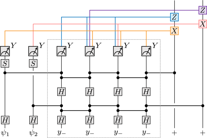
Figure 7: Standard teleportation of $k=2$ logical qubits using a modification of the generalized cluster state $\lvert C^{\,}_{2}\rangle$ (77). The conditioning of the recovery operations on the measurements is indicated by color-coded lines. The region within the dotted box is precisely the “bulk” resource state $\lvert C^{\,}_{2}\rangle$ (77), where the operations outside the dotted box capture the required modifications near the boundaries.

We first consider an extension of the cluster-state teleportation protocol discussed in Secs. 2.4 and 6.1 Briegel and Raussendorf (2001) to $k\geq 1$ Stephen et al. (2022). We present a family of SPT states $\lvert C^{\,}_{k}\rangle$ (77) with protecting symmetry $\mathcal{G}=\mathbb{Z}_{2}^{2k}$ (as required by Theorem 18), and which is closely related to other families of resource states known to be compatible with $k$-qubit teleportation Raussendorf et al. (2022); Stephen et al. (2022).

For convenience of presentation, we first define the extended “$k$-fold” cluster state in the bulk of the chain,

$$\lvert C^{\vphantom{\prime}}_{k}\rangle\equiv\bigg{(}\prod_{j}\mathrm{CZ}^{\,}_{j,j+1}\,\prod_{j^{\prime}}H^{\,}_{j^{\prime}}\bigg{)}^{k}\,\lvert y_{-}y_{-}\cdots y_{-}\rangle\,,~{}$$ (77)

where $H^{\,}_{j}=(X^{\vphantom{*}}_{j}+Z^{\vphantom{*}}_{j})/\sqrt{2}$ is the Hadamard gate, and the $+1$ eigenstates $\lvert+\rangle$ of $X^{\vphantom{*}}$ in Eq. 20 have been replaced by the $-1$ eigenstates $\lvert y_{-}\rangle$ of $Y^{\vphantom{*}}$, where $\lvert y_{\pm}\rangle=(\lvert 0\rangle\pm\mathrm{i}\,\lvert 1\rangle)/\sqrt{2}$ in the computational ($Z^{\vphantom{*}}$) basis. We note that the $k=1$ state $\lvert C^{\,}_{1}\rangle$ (77) is unitarily equivalent to the standard cluster state Briegel and Raussendorf (2001) via a $Z^{\vphantom{*}}$-basis rotation of all qubits by $\pi/4$. The stabilizer group $\operatorname*{stab}\left(*\right){\lvert C^{\,}_{k}\rangle}$ is generated by the operators

$$\mathsf{S}^{\vphantom{\prime}}_{j}=Z^{\vphantom{*}}_{j}\,Y^{\vphantom{*}}_{j+1}\cdots Y^{\vphantom{*}}_{j+2k-1}\,Z^{\vphantom{*}}_{j+2k}\,,~{}~{}$$ (78)

which bears some resemblance to Eq. 67. Furthermore, $\lvert C^{\,}_{k}\rangle$ (77) has a $\mathbb{Z}_{2}^{2k}$ symmetry generated by

$$g^{\vphantom{\prime}}_{p}=\prod\limits_{j}\,Y^{\vphantom{*}}_{2\,k\,j+p}\,,~{}~{}$$ (79)

for $p\in[1,2\,k]$. Hence, these $k$-fold cluster states can be used to teleport $k$ logical qubits via bulk measurements in local $Y$-basis, as depicted in Fig. 7 for $k=2$ and a single “measurement region” of size $2k$ in the bulk. The color-coded lines indicate how the measurement outcomes determine the recovery operations on $F$.

Importantly, we note that the resource state $\lvert\Psi^{\,}_{t}\rangle$ for teleportation requires modifying $\lvert C^{\,}_{k}\rangle$ (77) in the vicinity of the initial and final logical sets $I$ and $F$. In the bulk of the chain (i.e., a distance $r>v\,T$ from both $I$ and $F$), the initial state $\lvert\Psi^{\,}_{0}\rangle$ is simply $\lvert y_{-}\rangle$ on each site, and the unitary $\mathcal{U}$ is identical to the one implicit in Eq. 77. The required modifications are shown explicitly in Fig. 7 for $k=2$ logical qubits. They include modifying (i) the initial state $\lvert\Psi^{\,}_{0}\rangle$ in $F$ according to $\lvert y_{-}\rangle\to\lvert+\rangle$; (ii) the unitary $\mathcal{U}$ in the region $I=\{1,2\}$ to include phase gates $S=\mathrm{diag}(1,\mathrm{i})$ in the computational basis; and (iii) the measurement channel $\mathcal{M}$ in the region $I$ to include $k=2$ additional measurements in $I$ (only the four measurements in the boxed “bulk” region in Fig. 7 repeat for $m>1$).

The important takeaway is that the resource state $\lvert\Psi^{\,}_{t}\rangle$ (36) is equivalent to $\lvert C^{\,}_{k}\rangle$ (77) in the bulk of the chain. By the same token, this state is compatible with Theorem 18 for any $k$, as the modifications to $\lvert C^{\,}_{k}\rangle$ (77) required for teleportation are localized to the two edges, and merely modify the endpoint operators, which anticommute as required. Although it is possible to work out the modifications required at the two edges (i.e., outside of the boxed region in Fig. 7) for any $k>2$, this is not particularly illuminating or instructive. Instead, we consider an alternative family of states with a systematic procedure for encoding the edges in Sec. 6.4.

6.4 Valence-bond states for $k\geq 1$ logical qubits

We now describe another family of resource states suitable for the standard teleportation of $k\geq 1$ logical qubits. In contrast to the generalized cluster states $\lvert C^{\,}_{k}\rangle$ (77) of Sec. 6.3, the unitary $\mathcal{U}$ that prepares the actual resource state $\lvert\Psi^{\,}_{t}\rangle$ is straightforwardly related to the unitary that prepares the corresponding bulk SPT state $\lvert V^{\,}_{k}\rangle$ (80).

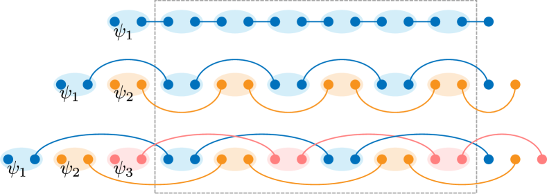
Figure 8: The valence-bond resource states for $k=1,2,3$ (top to bottom), where two dots connected by a line denote the Bell state $\lvert\mathrm{Bell}\rangle$. The bulk states in the dotted box realize $\lvert V^{\,}_{k}\rangle$ (80), which are closely related to the resource state $\lvert\Psi^{\,}_{t}\rangle$ (36) for teleportation. Performing Bell-basis $XX$ and $ZZ$ measurement on each oval teleports the qubits to the rightmost end points of Bell states, up to Pauli errors.

We refer to this family of states as valence-bond states, due to their resemblance to, e.g., the Affleck-Kennedy-Lieb-Tasaki (AKLT) state Affleck et al. (1987). These states are also closely related to the $\alpha$ chains introduced in Ref. 65. Given a 1D chain with an even number of qubits $N$, we define the $k$-fold valence bond state $\lvert V^{\,}_{k}\rangle$ (80) as

$$\lvert V^{\vphantom{\prime}}_{k}\rangle\equiv\bigotimes_{j}\,\lvert\mathrm{Bell}\rangle^{\vphantom{\prime}}_{2j,2j+2k-1}\,,~{}~{}$$ (80)

where $\lvert\mathrm{Bell}\rangle^{\,}_{a,b}=(\lvert 00\rangle^{\,}_{a,b}+\lvert 11\rangle^{\,}_{a,b})/\sqrt{2}$. These states are depicted in Fig. 8 for $k=1,2,3$, where the dotted box encloses the bulk of the chain. The states $\lvert V^{\,}_{k}\rangle$ (80) are symmetric under the group $\mathcal{G}=\mathbb{Z}_{2}^{2k}$ generated by

$$g^{x}_{p} =\prod\limits_{j}\,X^{\vphantom{*}}_{2\,k\,j+2\,p}\,X^{\vphantom{*}}_{2\,k\,j+2\,p+1}$$ (81a)

$$g^{z}_{p} =\prod\limits_{j}\,Z^{\vphantom{*}}_{2\,k\,j+2\,p}\,Z^{\vphantom{*}}_{2\,k\,j+2\,p+1}$$ (81b)

for $p\in[1,k]$. The corresponding string order parameters (63) act as one of the two generators (81) in the the bulk.

We now describe the valence-bond teleportation protocol. Given $k\geq 1$ logical qubits and a target distance $L^{\,}_{*}$ (13), we choose the minimum number of measurement regions $m\geq 1$ such that $L=\left(2\,m+1\right)k+1\geq L^{\,}_{*}$. These protocols involve at most nearest-neighbor gates (with $v=1$), and are optimal in that they use the minimum required depth $T=k+1$ (48), so that $L=T+2\,m\,(T-1)$ saturates the teleportation bound (47).

The protocol is implemented on a 1D chain with $N=(2\,m+3)k$ qubits. These qubits can be partitioned into a “bulk” region with $2\,k\,m$ qubits (the region enclosed in the dotted box in Fig. 8) along with an additional $2\,k$ qubits to the left of the bulk region and another $k$ qubits to the right. The system is initialized in the state

$$\lvert\Psi^{\vphantom{\prime}}_{0}\rangle =\prod\limits_{n=1}^{k}\lvert\psi^{\vphantom{\prime}}_{n}\rangle^{\vphantom{\prime}}_{2n-1}\otimes\lvert 0\rangle^{\vphantom{\prime}}_{2n}\otimes\prod\limits_{j=2k+1}^{N}\lvert 0\rangle^{\vphantom{\prime}}_{j}\,,~{}~{}$$ (82)

where $\lvert\psi^{\,}_{n}\rangle$ is the $n$th logical state on site $i_{n}=2n-1$. All bulk qubits $j\in[2k+1,2(m+1)k]$ are prepared in the initial state $\lvert 0\rangle$, though the sites $j=i_{n}+1$ and $j=N-n$ for $n\in[1,k]$ may be prepared in any state.

The resource state $\lvert\Psi^{\,}_{t}\rangle$ (36) for teleportation is prepared in $T=k+1$ layers of unitary evolution labelled $\mathcal{U}^{\,}_{p}$ for $p\in[0,k]$. While the valence-bond state $\lvert V^{\,}_{k}\rangle$ (80) is prepared by the first $k$ layers alone, the final unitary layer $\mathcal{U}^{\,}_{k}$ merely converts the symmetry generators in Eq. 81 into on-site operators, so both states are SPTs).

The first unitary layer is given by

$$\mathcal{U}^{\vphantom{\dagger}}_{0} =\Big{(}\prod\limits_{n=1}^{k}\,\mathrm{SWAP}^{\vphantom{\dagger}}_{2n-1,2n}\,\Big{)}\,\Bigg{[}\prod\limits_{j=k+1}^{(m+1)k}\,\mathcal{B}^{\vphantom{\dagger}}_{2j-1,2j}\,\Bigg{]}\,\mathds{1}\,,$$ (83)

corresponding to (i) the $2\,k$ sites on the left, (ii) the $2\,m\,k$ sites in the bulk, and (iii) the $k$ sites on the right, respectively, where $\mathrm{SWAP}\,\lvert a,b\rangle=\lvert b,a\rangle$ and, for convenience, we define the Bell encoding channel $\mathcal{B}$ as

$$\mathcal{B}^{\vphantom{\dagger}}_{a,b}\equiv\mathrm{CNOT}\left(a\to b\right)\,H^{\vphantom{\dagger}}_{a}\,,~{}~{}$$ (84)

where $\mathrm{CNOT}\left(a\to b\right)$ flips the $Z^{\vphantom{*}}$ state of qubit $b$ if qubit $a$ is in the $Z^{\vphantom{*}}$ state $\lvert 1\rangle$, and acts trivially otherwise, so that $\mathcal{B}^{\,}_{a,b}\,\lvert 00\rangle^{\,}_{a,b}=\lvert\mathrm{Bell}\rangle^{\,}_{a,b}$. Note that the SWAP gates in $\mathcal{U}^{\,}_{0}$ (83) can be omitted if we swap the states of sites $2n-1$ and $2n$ in $\lvert\Psi^{\,}_{0}\rangle$ (82), at the cost of decreasing $L$ (13) by one. When preparing the valence-bond state $\lvert V^{\,}_{k}\rangle$ (80) directly, $\mathcal{U}^{\,}_{0}$ only contains the bulk term in Eq. 83.

The next layers of $\mathcal{U}$ are given by

$$\mathcal{U}^{\vphantom{\dagger}}_{p}=\begin{cases}\prod\limits_{j=1}^{(m+1)k^{\vphantom{\dagger}}}\,\mathrm{SWAP}^{\vphantom{\dagger}}_{2j+2p-2,2j+2p-1}\,&\,p~{}{\rm odd}\\[2.0pt] \prod\limits_{j=1}^{(m+1)k}\,\mathrm{SWAP}^{\vphantom{\dagger}}_{2j+2p-3,2j+2p-2}\,&\,p~{}{\rm even}\end{cases}\,,~{}~{}$$ (85)

which can be thought of more simply as alternating layers of SWAP gates on even versus odd bonds, where the first layer of SWAP gates acts on even bonds—i.e., the SWAP gates in $\mathcal{U}^{\,}_{1}$ (85) are staggered by one site with respect to the Bell encoding channels $\mathcal{B}$ in $\mathcal{U}^{\,}_{0}$ (83).

The product of the untiaries $\mathcal{U}^{\,}_{k-1}\cdots\mathcal{U}^{\,}_{0}$ map the state $\lvert\boldsymbol{0}\rangle$ to the valence-bond state $\lvert V^{\,}_{k}\rangle$ (80). The analogous state $\lvert\Psi^{\,}_{T-1}\rangle$ for teleportation is captured by Fig. 8 for $k=1,2,3$; however, writing a general expression is inconvenient. The final layer of unitary evolution applies the Bell decoding channel to the qubits in ovals in Fig. 8, and SWAP gates to all qubits on the right end, i.e.,

$$\mathcal{U}^{\vphantom{\dagger}}_{k}=\prod\limits_{j=1}^{km}\mathcal{B}^{\dagger}_{k+2j-1,k+2j}\,\prod\limits_{n=0}^{k-1}\mathrm{SWAP}^{\vphantom{\dagger}}_{N-2n-1,N-2n},$$ (86)

where the SWAP gates on the final $2k$ sites can be omitted at the cost of decreasing $L$ (13) by one. Following the application of all unitaries, one measures $Z^{\vphantom{*}}_{j}$ on all sites $[k+1,(2m+1)k]$, where every $2k$ consecutive outcomes are determine recovery channels according to $(m_{x,1},m_{z,1},m_{x,2},m_{z,2},\dots,m_{x,k},m_{z,k})$, where $\sigma^{z/x}_{f_{n}}$ is applied to $f_{n}$ if $\sum_{s=1}^{m}m_{x/z,s}\cong 1$ mod $2$.

7 Outlook

We have shown that all “standard” teleportation protocols that teleport $k$ logical states a distance $L>vT$ (13) are equivalent to preparing a resource state with nontrivial SPT order protected by the symmetry $\mathcal{G}=\mathbb{Z}_{2}^{2k}$ (65) using local unitary evolution for time $T\ll L$, measuring the $2k$ string order parameters (63) in the bulk, and applying Pauli recovery gates (34) based on the outcomes. These protocols are physical in that the logical states $\lvert\psi^{\,}_{n}\rangle$ are realized on particular physical qubits. We require that no unitaries are applied to a site after it is measured, though we expect that this requirement can be relaxed.

The crucial feature of standard teleportation protocols from the perspective of constraining the resource state is that all outcome-dependent operations are Pauli gates. The recovery group—generated by all physical error-correction operators $\chi$ in $\mathcal{R}$ (18), modulo complex phases—is simply the $k$-qubit Pauli group $\mathbf{P}^{\vphantom{*}}_{*}{k}/\mathsf{U}\left(1\right)$ for standard teleportation, which forms a projective representation of the symmetry group $\mathcal{G}=\mathbb{Z}_{2}^{2k}$ (65). We expect that our analysis can be extended, mutatis mutandis, to more general recovery operations.

In this sense, our results (namely, Theorem 18) represent a first step toward classifying all quantum teleportation protocols based solely on their recovery (or decoding) channels (18). There are numerous recovery operations to consider beyond the Paulis of standard teleportation: The corresponding group can be continuous and non-Abelian (i.e., $\chi^{\,}_{g}\,\chi^{\,}_{h}\neq\omega(g,h)\,\chi^{\,}_{h}\,\chi^{\,}_{g}$ for some complex phase $\omega$). We can also condition measurements (or the basis of a measurement) on prior outcomes, and condition operations on the outcomes of measurements in other ways (e.g., nonlinearly). For example, Ref. 66 considers Pauli recovery operations but does not require that they be conditioned on outcome parities, in which case the resource states can be chosen to have SPT order, but the symmetry generators $U(g)$ are no longer “on site” (49). Alternatively, one might consider non-Abelian—and even continuous—recovery groups, whose corresponding resource states are matrix product states Gross and Eisert (2007, 2010) that generally do not have string order Popp et al. (2005). We expect that our methods using the Stinespring formalism will be crucial in analyzing these more exotic protocols and their potential relation to exotic forms of SPT order.

Appendix A Proof of Proposition 1

Proof.

For the teleportation conditions 8 to be necessary and sufficient for quantum state transfer (see Def. 1), they must be equivalent to (5) for the initial state $\lvert\Psi^{\,}_{0}\rangle$ (6) and final state $\lvert\Psi^{\,}_{T}\rangle$ (7). We prove both directions of implication in turn, using the fact that all operators acting on a qubit can be decomposed onto the Pauli operators $\mathds{1},X^{\vphantom{*}},Y^{\vphantom{*}},Z^{\vphantom{*}}$, which are spanned by $X^{\vphantom{*}}$ and $Z^{\vphantom{*}}$. The coefficients $\alpha$ and $\beta$ of a logical state $\lvert\psi\rangle$ can be extracted from the expectation values of the Pauli operators (4).

We first establish that Eqs. 5, 6, and 7 imply Eq. 8—i.e., Eq. 8 is necessary for state transfer. First, Eq. 7 implies that $X^{\vphantom{*}}_{f_{n}}$ is the $X^{\vphantom{*}}$-type logical operator for the $n$th logical qubit acting on the final state $\lvert\Psi^{\,}_{T}\rangle$ (7), as it interchanges $\alpha^{\,}_{n}$ and $\beta^{\,}_{n}$. In the Heisenberg picture, this logical operator evolves under $\mathcal{W}$ according to

$$X^{(n)}_{{\rm L}}(T)\,=\,X^{\vphantom{*}}_{f_{n}}(T)\,=\,\mathcal{W}^{\dagger}\,X^{\vphantom{*}}_{f_{n}}\,\mathcal{W}\,,~{}~{}$$ (A.87)

and now, using the fact that $X^{2}_{i_{n}}=\mathds{1}$ is involutory, we introduce an arbitrary operator $\mathsf{S}^{\,}_{n,x}$ via

$$X^{(n)}_{{\rm L}}(T)\, =\,\mathds{1}\,\mathcal{W}^{\dagger}X^{\vphantom{*}}_{f_{n}}\mathcal{W}\,=\,X^{2}_{i_{n}}\,\mathcal{W}^{\dagger}X^{\vphantom{*}}_{f_{n}}\mathcal{W}$$

$$=\,X^{\vphantom{*}}_{i_{n}}\,\left(X^{\vphantom{*}}_{i_{n}}\,\mathcal{W}^{\dagger}X^{\vphantom{*}}_{f_{n}}\mathcal{W}\right)\,\equiv\,X^{\vphantom{*}}_{i_{n}}\,\mathsf{S}^{\,}_{n,x}\,,~{}~{}$$ (A.88)

which implicitly defines the (unitary) operator $\mathsf{S}^{\,}_{n,x}$ as

$$\mathsf{S}^{\,}_{n,x}\,\equiv\,X^{\vphantom{*}}_{i_{n}}\,\mathcal{W}^{\dagger}X^{\vphantom{*}}_{f_{n}}\mathcal{W}\,.$$ (A.89)

Leaving the coefficients $\alpha^{\,}_{j},\beta^{\,}_{j}$ for $j\neq n$ implicit for convenience, we apply $\mathsf{S}^{\,}_{n,x}$ (A.89) to the initial state $\lvert\Psi^{\,}_{0}(\alpha^{\,}_{n},\beta^{\,}_{n})\rangle$ (6) and use the first part of Eq. 5 to find

$$\mathsf{S}^{\,}_{n,x}\,\lvert\Psi^{\vphantom{\prime}}_{0}(\alpha^{\,}_{n},\beta^{\,}_{n})\rangle\, =\,X^{\vphantom{*}}_{i_{n}}\,\mathcal{W}^{\dagger}X^{\vphantom{*}}_{f_{n}}\mathcal{W}\,\lvert\Psi^{\vphantom{\prime}}_{0}(\alpha^{\,}_{n},\beta^{\,}_{n})\rangle$$

$$=\,X^{\vphantom{*}}_{i_{n}}\,\mathcal{W}^{\dagger}X^{\vphantom{*}}_{f_{n}}\lvert\Psi^{\vphantom{\prime}}_{T}(\alpha^{\,}_{n},\beta^{\,}_{n})\rangle$$

$$=\,X^{\vphantom{*}}_{i_{n}}\,\mathcal{W}^{\dagger}\lvert\Psi^{\vphantom{\prime}}_{T}(\beta^{\,}_{n},\alpha^{\,}_{n})\rangle$$

$$=\,X^{\vphantom{*}}_{i_{n}}\lvert\Psi^{\vphantom{\prime}}_{0}(\beta^{\,}_{n},\alpha^{\,}_{n})\rangle$$

$$=\,\lvert\Psi^{\vphantom{\prime}}_{0}(\alpha^{\,}_{n},\beta^{\,}_{n})\rangle\,,~{}~{}$$ (A.90)

meaning that $\mathsf{S}^{\,}_{n,x}$ (A.89) is an element of the initial-state stabilizer group $\operatorname*{stab}\left(*\right){\lvert\Psi^{\,}_{0}\rangle}$ (3), and is guaranteed to be unitary. Next, applying the Heisenberg-evolved operator $X^{\vphantom{*}}_{f_{n}}(T)$ (A.87) to the initial state $\lvert\Psi^{\,}_{0}\rangle$ (6) gives

$$X^{(n)}_{{\rm L}}(T)\,\lvert\Psi^{\vphantom{\prime}}_{0}(\alpha^{\,}_{n},\beta^{\,}_{n})\rangle\, =\,X^{\vphantom{*}}_{i_{n}}\,\mathsf{S}^{\,}_{n,x}\,\lvert\Psi^{\vphantom{\prime}}_{0}(\alpha^{\,}_{n},\beta^{\,}_{n})\rangle$$

$$=\,X^{\vphantom{*}}_{i_{n}}\,\lvert\Psi^{\vphantom{\prime}}_{0}(\alpha^{\,}_{n},\beta^{\,}_{n})\rangle\,,~{}~{}$$ (A.91)

which holds for any choice of $\alpha^{\,}_{n},\beta^{\,}_{n}$. This implies that $X^{(n)}_{{\rm L}}(T)\,=\,\mathcal{W}^{\dagger}\,X^{\vphantom{*}}_{f_{n}}\,\mathcal{W}\,$ realizes an $X^{\vphantom{*}}$-type logical operator for the $n$th logical qubit acting on the initial state $\lvert\Psi^{\,}_{0}\rangle$ (6)—i.e., it acts as $X^{\vphantom{*}}_{i_{n}}$ times some stabilizer $\mathsf{S}^{\,}_{n,x}$ (A.89), where the latter acts trivially on $\lvert\Psi^{\,}_{0}\rangle$ (6).

An analogous procedure applies to the $Z^{\vphantom{*}}$-type logical operator for the $n$th logical qubit. That operator evolves in the Heisenberg picture according to

$$Z^{(n)}_{{\rm L}}(T)\,=\,Z^{\vphantom{*}}_{f_{n}}(T)\,=\,\mathcal{W}^{\dagger}\,Z^{\vphantom{*}}_{f_{n}}\,\mathcal{W}\,,~{}~{}$$ (A.92)

in analogy to Eq. A.87, and implied by Eq. 7. We then define another stabilizer $\mathsf{S}^{\,}_{n,z}\equiv Z^{\vphantom{*}}_{i_{n}}\,\mathcal{W}^{\dagger}Z^{\vphantom{*}}_{f_{n}}\mathcal{W}$, implying that $\mathsf{S}^{\,}_{n,z}$ is also an element of $\operatorname*{stab}\left(*\right){\lvert\Psi^{\,}_{0}\rangle}$ (3). Applying the logical $Z^{\vphantom{*}}$ operator (A.92) to $\lvert\Psi^{\,}_{0}\rangle$ (6) reveals that

$$Z^{(n)}_{{\rm L}}(T)=\mathcal{W}^{\dagger}\,Z^{\vphantom{*}}_{f_{n}}\,\mathcal{W}=Z^{\vphantom{*}}_{i_{n}}\,\mathsf{S}^{\,}_{n,z}\,,~{}~{}$$ (A.93)

is the $Z^{\vphantom{*}}$-type logical operator for the $n$th logical qubit acting on the initial state $\lvert\Psi^{\,}_{0}\rangle$ (6), in analogy to Eq. A.91.

Thus, the fact that $\mathcal{W}$ teleports $k$ logical states in the Schrödinger picture via EQ. 5 implies that (i) $\mathcal{W}$ teleports $k$ pairs of logical operators in the Heisenberg picture; (ii) $X^{(n)}_{{\rm L}}(T)\,=\,\mathcal{W}^{\dagger}\,X^{\vphantom{*}}_{f_{n}}\,\mathcal{W}\,=\,X^{\vphantom{*}}_{i_{n}}\,\mathsf{S}^{\vphantom{\prime}}_{n,x}$ and $Z^{(n)}_{{\rm L}}(T)\,=\,\mathcal{W}^{\dagger}\,Z^{\vphantom{*}}_{f_{n}}\,\mathcal{W}\,=\,Z^{\vphantom{*}}_{i_{n}}\,\mathsf{S}^{\vphantom{\prime}}_{n,z}$ are valid $X^{\vphantom{*}}$- and $Z^{\vphantom{*}}$-type logical operators for the $n$th logical qubit acting on the initial state $\lvert\Psi^{\,}_{0}\rangle$ (6); and (iii) the operators $\mathsf{S}^{\,}_{n,x}$ and $\mathsf{S}^{\,}_{n,z}$ are elements of the initial-state stabilizer group $\operatorname*{stab}\left(*\right){\lvert\Psi^{\,}_{0}\rangle}$ (3). Hence, Eq. 5 implies Eq. 8.

Now, we prove the reverse implication: Any protocol $\mathcal{W}$ satisfying Eq. 8 with the initial state $\lvert\Psi^{\,}_{0}\rangle$ (6) implies state transfer (5) with final state $\lvert\Psi^{\,}_{T}\rangle$ (7)—i.e., Eq. 8 is sufficient for Eq. 5. For convenience, we define

$$\rho^{\vphantom{\dagger}}_{n}\, =\,\lvert\psi^{\,}_{n}\rangle\langle\psi^{\,}_{n}\rvert$$

$$=\,\frac{1}{2}\mathds{1}+c^{(n)}_{1}\,X^{\vphantom{*}}_{i_{n}}++c^{(n)}_{2}\,Y^{\vphantom{*}}_{i_{n}}+c^{(n)}_{3}\,Z^{\vphantom{*}}_{i_{n}}$$

$$=\,\frac{1}{2}\left(\mathds{1}+\sum_{\nu=1}^{3}c^{(n)}_{\nu}\sigma^{\nu}_{i_{n}}\right)\,,~{}$$ (A.94)

where the coefficients $c^{(n)}_{\nu}$ are given by

$$c^{(n)}_{\nu}\, \equiv\,\left\langle\psi^{\,}_{n}\middle|\sigma^{\nu}_{i_{n}}\middle|\psi^{\,}_{n}\right\rangle\,,~{}~{}$$ (A.95)

for the $n$th logical qubit, as in Eq. 4. We can then write the initial density matrix associated with $\lvert\Psi^{\,}_{0}\rangle$ (6) as

$$\rho^{\,}_{0} =\lvert\Psi^{\vphantom{\prime}}_{0}\left(\boldsymbol{\alpha},\boldsymbol{\beta}\right)\rangle\langle\Psi^{\vphantom{\prime}}_{0}\left(\boldsymbol{\alpha},\boldsymbol{\beta}\right)\rvert\,$$

$$=\left[\prod\limits_{n=1}^{k}\,\rho^{\vphantom{\dagger}}_{n}\right]\otimes\lvert\Phi^{\vphantom{\prime}}_{i}\rangle\langle\Phi^{\vphantom{\prime}}_{i}\rvert^{\vphantom{\dagger}}_{\rm rest}\,,$$ (A.96)

which realizes $\rho^{\,}_{n}=\lvert\psi^{\,}_{n}\rangle\langle\psi^{\,}_{n}\rvert$ on each initial logical qubit $i_{n}$. Using Eqs. A.96 and A.94, we write

$$\mathcal{W}\,\lvert\Psi^{\vphantom{*}}_{i}\rangle =\mathcal{W}\,\lvert\psi^{\,}_{n}\rangle\langle\psi^{\,}_{n}\rvert^{\vphantom{*}}_{i_{n}}\lvert\Psi^{\vphantom{*}}_{i}\rangle$$

$$=\mathcal{W}\,\frac{1}{2}\left(\mathds{1}+\sum_{\nu=1}^{3}c^{(n)}_{\nu}\sigma^{\nu}_{i_{n}}\right)\lvert\Psi^{\vphantom{*}}_{i}\rangle$$

$$=\mathcal{W}\,\frac{1}{2}\left(\mathds{1}+\sum_{\nu=1}^{3}c^{(n)}_{\nu}\sigma^{\nu}_{i_{n}}\mathsf{S}^{\,}_{n,\nu}\right)\lvert\Psi^{\vphantom{*}}_{i}\rangle$$

$$=\mathcal{W}\,\frac{1}{2}\left(\mathds{1}+\sum_{\nu=1}^{3}c^{(n)}_{\nu}\mathcal{W}^{\dagger}\sigma^{\nu}_{f_{n}}\,\mathcal{W}\right)\lvert\Psi^{\vphantom{*}}_{i}\rangle$$

$$=\frac{1}{2}\left(\mathds{1}+\sum_{\nu=1}^{3}c^{(n)}_{\nu}\sigma^{\nu}_{f_{n}}\right)\mathcal{W}\,\lvert\Psi^{\vphantom{*}}_{i}\rangle$$

$$=\lvert\psi^{\,}_{n}\rangle\langle\psi^{\,}_{n}\rvert^{\vphantom{*}}_{f_{n}}\,\mathcal{W}\,\lvert\Psi^{\vphantom{*}}_{i}\rangle\,,~{}~{}$$ (A.97)

where the second line follows from Eq. A.94; the third line uses $\mathsf{S}^{\,}_{n,\nu}\in\operatorname*{stab}\left(*\right){\lvert\Psi^{\,}_{0}\rangle}$ to insert stabilizers inside the parenthetical expression; the fourth line uses Eqs. 8 and 9; and the last line uses Eq. A.94 once again. Thus, the final state $\lvert\Psi^{\,}_{T}\rangle=\mathcal{W}\,\lvert\Psi^{\,}_{0}\rangle$ (7) is stabilized by the $n$th logical qubit’s density matrix on site $f^{\,}_{n}$. For brevity, we represent the final density matrix as $\rho^{\,}_{T}=\mathcal{W}\,\lvert\Psi^{\,}_{0}\rangle\langle\Psi^{\,}_{0}\rvert\mathcal{W}^{\dagger}$. Since $\lvert\psi^{\,}_{n}\rangle\langle\psi^{\,}_{n}\rvert^{\,}_{f_{n}}$ only acts nontrivially on site $f_{n}$, we have

$$1 ={\rm tr}\left[\,\rho^{\vphantom{*}}_{T}\,\right]={\rm tr}\left[\,\lvert\psi^{\,}_{n}\rangle\langle\psi^{\,}_{n}\rvert^{\vphantom{*}}_{f_{n}}\,\rho^{\vphantom{*}}_{T}\,\right]$$

$$={\rm tr}\left[\,\lvert\psi^{\,}_{n}\rangle\langle\psi^{\,}_{n}\rvert\,\rho^{\vphantom{*}}_{f_{n}}\,\right]=F\left(\rho^{\vphantom{*}}_{f_{n}},\lvert\psi^{\vphantom{*}}_{n}\rangle\right)\,,~{}$$ (A.98)

where $F$ is the fidelity Jozsa (1994), and in second line we used Eq. A; in the third line we have defined $\rho^{\,}_{f_{n}}\equiv\operatorname*{tr}^{\,}_{f^{c}_{n}}\left[\,\rho^{\,}_{T}\,\right]$ as the reduced final density matrix on site $f_{n}$; in the last line we have used the fact that the fidelity obeys $F(\rho,\lvert\psi\rangle)=\left\langle\psi\middle|\rho\middle|\psi\right\rangle={\rm tr}\left[\,\lvert\psi\rangle\langle\psi\rvert\,\rho\,\right]$ when one of the states is pure Jozsa (1994). Note that, in the second line the trace is over the entire system, whereas in the third line, it is only over $f_{n}$. Since $F(\rho^{\vphantom{*}}_{f_{n}},\lvert\psi^{\vphantom{*}}_{n}\rangle)=1$, we must have that

$$\rho^{\vphantom{*}}_{f_{n}}=\operatorname*{tr}^{\,}_{f^{c}_{n}}\left[\,\rho\,\right]=\lvert\psi^{\,}_{n}\rangle\langle\psi^{\,}_{n}\rvert\,,~{}$$ (A.99)

i.e., the final reduced density matrix on site $f_{n}$ is the logical $n$th (pure) state. Since the above arguments hold for all $n=1,\dots,k$ independently, we conclude that $\lvert\Psi^{\,}_{T}\rangle=\mathcal{W}\,\lvert\Psi^{\,}_{0}\rangle$ satisfies (5) for the final state $\lvert\Psi^{\,}_{T}\rangle$ (7). Thus, Eq. 8 is both necessary and sufficient for Eq. 5. ∎

Appendix B Proof of Proposition 4

Proof.

A generic and nontrivial single-qubit observable $A^{\,}_{j}$ is guaranteed to have exactly two unique eigenvalues $a^{\,}_{0}>a^{\,}_{1}$, with spectral decomposition (15)

$$A^{\vphantom{\dagger}}_{j} =a^{\,}_{0}\,P^{(0)}_{j}+a^{\,}_{1}\,P^{(1)}_{j}\,,~{}~{}$$ (B.100)

which we decompose onto the Pauli basis via

$$A^{\vphantom{\prime}}_{j} =\frac{1}{2}\,\sum\limits_{\nu=0}^{3}\,\operatorname*{tr}\limits_{j}\,\left[\,A^{\vphantom{\prime}}_{j}\,\sigma^{\nu}_{j}\,\right]\,\sigma^{\nu}_{j}$$

$$=\frac{1}{2}\left(a^{\,}_{0}+a^{\,}_{1}\right)\,\mathds{1}+\vec{\alpha}^{\vphantom{\prime}}_{j}\cdot\vec{\sigma}^{\vphantom{\prime}}_{j}\,,~{}~{}$$ (B.101)

where $\vec{\sigma}^{\,}_{j}=(X^{\vphantom{*}}_{j},Y^{\vphantom{*}}_{j},Z^{\vphantom{*}}_{j})$ is a vector of Pauli matrices and $\vec{\alpha}^{\,}_{j}$ is a vector of coefficients as determined by the Pauli decomposition. Importantly, using the properties of $2\times 2$ matrices and the fact that $\det\,\left[A^{\,}_{j}\right]=a^{\,}_{0}\,a^{\,}_{1}$ we find

$$\lvert\vec{\alpha}\rvert=\frac{1}{2}\lvert a^{\,}_{0}-a^{\,}_{1}\rvert\,,~{}~{}$$ (B.102)

for the magnitude of $\vec{\alpha}$. This provides for the definition of a unit vector $\hat{\alpha}$ that is parallel to the original vector $\vec{\alpha}$.

We rewrite the decomposed observable $A^{\,}_{j}$ (B.101) as

$$A^{\vphantom{\dagger}}_{j} =\frac{1}{2}\left(a^{\,}_{0}+a^{\,}_{1}\right)\,\mathds{1}+\frac{1}{2}\left(a^{\,}_{0}-a^{\,}_{1}\right)\,\sum\limits_{n=1}^{3}\,\hat{\alpha}^{\vphantom{\prime}}_{j,n}\,\sigma^{n}_{j}$$

$$=\frac{1}{2}\operatorname*{tr}\limits_{j}\left[A^{\vphantom{\prime}}_{j}\right]\,\mathds{1}+\frac{1}{2}\,\left(a^{\,}_{0}-a^{\,}_{1}\right)\,\bar{A}^{\vphantom{\prime}}_{j}\,,~{}~{}$$ (B.103)

where the vector $\hat{\alpha}^{\,}_{j}=(\hat{\alpha}^{\,}_{j,1},\hat{\alpha}^{\,}_{j,2},\hat{\alpha}^{\,}_{j,3})$ is real valued and has unit length. This expression agrees with Eq. 33.

We next recover simple expressions for the projectors $P^{(n)}_{j}$ (B.100) onto the states (or spaces of states) with eigenvalues $a^{\,}_{n}$. We first note that these two projectors must be orthogonal for the eigenvalue equation $A^{\,}_{j}\,P^{(n)}_{j}=a^{\,}_{n}\,P^{(n)}_{j}$ to hold. Second, we note that these two projectors must be complete (i.e., sum to the identity), or else evaluating $\det\,\left[A^{\,}_{j}\right]$ in the eigenbasis of $A^{\,}_{j}$ would return zero, independent of the values of $a^{\,}_{0,1}$. As a result,

$$A^{\vphantom{\dagger}}_{j} =a^{\,}_{n}\,P^{(n)}_{j}+a^{\,}_{1-n}\left(\mathds{1}-P^{(n)}_{j}\right)$$

$$=a^{\,}_{1-n}\,\mathds{1}+\left(a^{\,}_{n}-a^{\,}_{1-n}\right)\,P^{(n)}_{j}\,,~{}~{}$$ (B.104)

for either $n=0,1$. Rearranging this expression gives

$$P^{(n)}_{j} =\left(a^{\,}_{n}-a^{\,}_{1-n}\right)^{-1}\,\left(A^{\vphantom{\prime}}_{j}-a^{\,}_{1-n}\,\mathds{1}\right)$$ (B.105)

$$=\frac{1}{a^{\,}_{n}-a^{\,}_{1-n}}\left(\frac{1}{2}\operatorname*{tr}\limits_{j}\left[A^{\vphantom{\prime}}_{j}\right]\mathds{1}+\lvert\vec{\alpha}\rvert\,\bar{A}^{\vphantom{\prime}}_{j}-a^{\,}_{1-n}\mathds{1}\right)$$

$$=\frac{1}{a^{\,}_{n}-a^{\,}_{1-n}}\left(\frac{1}{2}(a^{\,}_{n}-a^{\,}_{1})\mathds{1}+\frac{1}{2}(a^{\,}_{0}-a^{\,}_{1})\,\bar{A}^{\vphantom{\prime}}_{j}\right)$$

$$=\frac{1}{2}\left(\mathds{1}+(-1)^{n}\,\bar{A}^{\vphantom{\prime}}_{j}\right)\,,~{}~{}$$ (B.106)

where we used Eq. B.101 to write $A^{\,}_{j}$ in terms of its involutory part $\bar{A}^{\,}_{j}$ (33), along with the relations $a^{\,}_{0}-a^{\,}_{1}=(-1)^{n}(a^{\,}_{n}-a^{\,}_{1-n})=2\lvert\vec{\alpha}\rvert$ (B.102) and $\operatorname*{tr}_{j}\left[A^{\,}_{j}\right]=a^{\,}_{0}+a^{\,}_{1}$.

Because the involutory operator $A^{\,}_{j}$ squares to the identity, its eigenvalues are $\pm 1$. Accordingly, the projectors onto eigenstates of $A^{\,}_{j}$ (which are also eigenstates of the original observable $A^{\,}_{j}$) are given by Eq. B.106. Intuitively, these observables must share eigenstates because they commute: They differ only by a scalar factor and an overall, universally commuting identity component. Finally, because only the projectors onto eigenstates of $A^{\,}_{j}$ appear in the unitary measurement channel (16), measurement of $A^{\,}_{j}$ is equivalent to measurement of $\bar{A}^{\,}_{j}$ (33). ∎

Appendix C Proof of Proposition 5

Proof.

At Heisenberg time $\tau=0$, the initial operator acts as $\Gamma\otimes\widetilde{\mathds{1}}^{\vphantom{*}}_{\rm ss}$ (i.e., trivially on all Stinespring registers). The outcome-averaged Heisenberg update to $\Gamma$ is given by

$$\Gamma^{\prime} =\operatorname*{tr}\limits_{{\rm ss},j}\,\left[\,\mathcal{M}^{\dagger}_{\left[A^{\,}_{j}\right]}\,\Gamma\otimes\widetilde{\mathds{1}}^{\vphantom{*}}_{j}\,\mathcal{M}^{\vphantom{\dagger}}_{\left[A^{\,}_{j}\right]}\,\widetilde{P}^{(0)}_{j}\,\right]\,,~{}~{}$$ (C.107)

since the $j$th Stinespring qubit is prepared in the $\lvert 0\rangle$ state by default. Using Eqs. 16 and B.106, the above becomes

$$\Gamma^{\prime} =\sum\limits_{m,n=0,1}\frac{1}{4}\left(\mathds{1}+(-1)^{m}\,\bar{A}^{\vphantom{\prime}}_{j}\right)\,\Gamma\,\left(\mathds{1}+(-1)^{m}\,\bar{A}^{\vphantom{\prime}}_{j}\right)$$

$$~{}~{}~{}\quad~{}~{}\times~{}{\rm tr}\left[\,\widetilde{X}^{m}_{j}\,\widetilde{\mathds{1}}^{\vphantom{*}}_{j}\,\widetilde{X}^{n}_{j}\,\widetilde{P}^{(n)}_{j}\,\right]$$

$$=\frac{1}{4}\sum\limits_{m=0,1}\,\left(\Gamma+(-1)^{m}\,\left\{\bar{A}^{\,}_{j},\,\Gamma\right\}+\bar{A}^{\,}_{j}\,\Gamma\,\bar{A}^{\,}_{j}\right)$$

$$=\frac{1}{4}\sum\limits_{m=0,1}\,\left(\bar{A}^{\,}_{j}+(-1)^{m}\,\mathds{1}\right)\,\left\{\bar{A}^{\,}_{j},\,\Gamma\right\}\,,~{}~{}$$ (C.108)

and if $\Gamma$ acts trivially (i.e., as the identity $\mathds{1}$) on qubit $j$, then we find $\Gamma^{\prime}=\Gamma$, meaning that the measurement did nothing, on average. However, if $\Gamma$ acts on qubit $j$ as $\sigma^{\nu}_{j}$, then Eq. C.108 can be rewritten

$$\Gamma^{\prime} =\frac{1}{2}\sum\limits_{m=0,1}\,(-1)^{m}\,P^{(m)}_{j}\,\sum\limits_{\mu=1}^{3}\,\hat{\alpha}^{\vphantom{\prime}}_{j,\mu}\,\left\{\sigma^{\mu}_{j},\,\sigma^{\nu}_{j}\right\}$$

$$=\sum\limits_{m=0,1}\,(-1)^{m}\,P^{(m)}_{j}\,\hat{\alpha}^{\vphantom{\prime}}_{j,\nu}=\operatorname*{tr}\limits_{j}\,\left[\,\bar{A}^{\vphantom{\prime}}_{j}\,\sigma^{\nu}_{j}\,\right]\,\bar{A}^{\vphantom{\prime}}_{j}\,,~{}~{}$$ (C.109)

which is neither involutory nor unitary, and thus incompatible with the teleportation conditions (8) imposed by, e.g., Def. 6 and Prop. 1. To see this, note that $\Gamma^{\prime}$ squares to ${\rm tr}\left[\bar{A}^{\,}_{j}\,\sigma^{\nu}_{j}\,\right]\,\mathds{1}$, which generically has operator norm (11) less than one. However, if $\bar{A}^{\,}_{j}=\sigma^{\mu}_{j}$, then $\Gamma^{\prime}$ (C.109) is either identically zero or equal to $\Gamma$ (if $\mu=\nu$).

In other words, if we evolve any logical operator $\Gamma$ (or Pauli-string observable of interest) under a dilated unitary channel $\mathcal{M}$ corresponding to projective measurement of a single-qubit observable $A^{\,}_{j}$ without outcome-dependent recovery operations, then the Heisenberg-evolved operator $\Gamma^{\prime}$ (C.107) realizes one of the following:

1. If the operator $\Gamma$ and $A^{\,}_{j}$ share no support, then $\Gamma^{\prime}=\Gamma$, meaning that $\mathcal{M}$ acts trivially.

2. If the involutory part of $A^{\,}_{j}$ and the Pauli content of $\Gamma$ on qubit $j$ are both $\sigma^{\mu}_{j}$, then $\Gamma^{\prime}=\Gamma$, so that $\mathcal{M}$ acts trivially.

3. If the involutory part of $A^{\,}_{j}$ and the Pauli content of $\Gamma$ on qubit $j$ correspond to distinct Pauli operators, then $\Gamma^{\prime}=0$, meaning that teleportation fails because the logical operator is destroyed.

4. If the involutory part of $A^{\,}_{j}$ realizes a superposition of Pauli operator (33), then $\Gamma^{\prime}$ is no longer involutory nor unitary, and thus cannot reproduce the logical operator algebra (8) acting on the initial state, which is required by Prop. 1.

In all cases above, either the measurement channel $\mathcal{M}$ acts trivially on a Pauli string $\Gamma$ of interest, or it causes teleportation to fail (because $\Gamma$ fails to be unitary). Hence, measurement without outcome-dependent recovery operations is not useful to quantum teleportation. ∎

Appendix D Proof of Proposition 6

Proof.

By construction, the logical reduced density matrix

$$\rho^{\vphantom{\prime}}_{\rm L}\equiv\operatorname*{tr}_{F^{c}}\left[\mathcal{W}\,\rho^{\vphantom{\prime}}_{0}\otimes\lvert\boldsymbol{0}\rangle\langle\boldsymbol{0}\rvert^{\vphantom{\prime}}_{\rm ss}\,\mathcal{W}^{\dagger}\right]\,,~{}~{}$$ (D.110)

is a pure state, and separable with respect to the partition $F|F^{c}$. In particular, $\lvert F\rvert=k$ is the number of logical qubits, and $\rho^{\,}_{\rm L}$ (D.110) is guaranteed to be unitarily equivalent to the pure state $\bigotimes_{n=1}^{k}\lvert\psi^{\,}_{n}\rangle\langle\psi^{\,}_{n}\rvert^{\,}_{n}$. Because $F^{c}$ includes all Stinespring qubits, $\rho^{\,}_{\rm L}$ (D.110) is implicitly averaged over the outcomes of all measurements in $\mathcal{W}$.

Additionally, the logical reduced density matrix $\rho^{\,}_{\rm L}$ (D.110) after realizing the sequence of measurement outcomes $\boldsymbol{n}=(n^{\,}_{1},\dots,n^{\,}_{M})$ is given by Friedman et al. (2022b); Barberena and Friedman (2023); Friedman et al. (2022a)

$$\rho^{(\boldsymbol{n})}_{\rm L}\equiv\frac{\operatorname*{tr}_{F^{c}}\left[\,\rho^{\vphantom{\prime}}_{T}\,\widetilde{P}^{(\boldsymbol{n})}_{\rm ss}\,\right]}{\operatorname*{tr}_{\rm dil}\left[\,\rho^{\vphantom{\prime}}_{T}\,\widetilde{P}^{(\boldsymbol{n})}_{\rm ss}\,\right]}\,,~{}~{}$$ (D.111)

where the denominator is equal to the the probability $p^{\,}_{\boldsymbol{n}}$ of the “outcome trajectory” $\boldsymbol{n}$.

Thus, the outcome-averaged logical reduced density matrix $\rho^{\,}_{\rm L}$ (D.110) is automatically a convex sum over trajectories $\boldsymbol{n}$ of the reduced density matrix $\rho^{(\boldsymbol{n})}_{\rm L}$ (D.111) weighted by the scalar $p^{\,}_{\boldsymbol{n}}$. However, such a density matrix is pure if and only if every term in the sum is proportional to $\rho^{\,}_{\rm L}$ (D.110). Because $\rho^{\,}_{\rm L}$ (D.110) and $\rho^{(\boldsymbol{n})}_{\rm L}$ (D.111) are proportional and normalized for all $\boldsymbol{n}$, we must have that $\rho^{(\boldsymbol{n})}_{\rm L}=\rho^{\vphantom{\prime}}_{\rm L}$ for all $\boldsymbol{n}$. Hence, the output state $\rho^{\,}_{\rm L}$ (D.110) is realized on all outcome trajectories. ∎

Appendix E Proof of Lemma 7

Proof.

Let $\mathcal{R}^{\,}_{s}$ be a recovery channel (34) and $\Gamma$ to be be any logical operator. By construction (and Def. 5), both $\chi^{\,}_{s}$ (34) and $\Gamma$ are Pauli-string operators (2). Evolving $\Gamma$ under $\mathcal{R}^{\,}_{s}$ in the Heisenberg picture gives

$$\mathcal{R}^{\dagger}_{s}\,\Gamma\otimes\widetilde{\mathds{1}}^{\vphantom{*}}\,\mathcal{R}^{\vphantom{\dagger}}_{s} =\sum\limits_{m,n=0,1}\,\chi^{m}_{s}\,\Gamma\,\chi^{n}_{s}\otimes\widetilde{P}^{(m)}_{r^{\,}_{s}}\,\widetilde{\mathds{1}}^{\vphantom{*}}\,\widetilde{P}^{(n)}_{r^{\,}_{s}}$$

$$=\sum\limits_{m=0,1}\,\chi^{m}_{s}\,\Gamma\,\chi^{m}_{s}\otimes\widetilde{P}^{(m)}_{r^{\,}_{s}}$$

$$=\sum\limits_{m=0,1}\,\left(-1\right)^{m\,\lambda^{\,}_{\Gamma,s}}\,\Gamma\otimes\widetilde{P}^{(m)}_{r^{\,}_{s}}$$

$$=\Gamma\otimes\left(\delta^{\,}_{\lambda^{\,}_{\Gamma,s},0}\,\widetilde{\mathds{1}}^{\vphantom{*}}+\delta^{\,}_{\lambda^{\,}_{\Gamma,s},1}\,\widetilde{Z}^{\vphantom{*}}_{r^{\,}_{s}}\right)$$

$$=\Gamma\otimes\widetilde{Z}^{\lambda^{\,}_{\Gamma,s}}_{r^{\,}_{s}}\,,~{}~{}$$ (E.112)

where $\widetilde{Z}^{\vphantom{*}}_{r^{\,}_{s}}$ is the product of $\widetilde{Z}^{\vphantom{*}}_{j}$ for $j\in r^{\,}_{s}$, where

$$\chi^{\vphantom{\dagger}}_{s}\,\Gamma\,\chi^{\vphantom{\dagger}}_{s}=\left(-1\right)^{\lambda^{\vphantom{\prime}}_{\Gamma,s}}\,\Gamma\,,~{}~{}$$ (E.113)

defines $\lambda^{\vphantom{\prime}}_{\Gamma,s}\in\{0,1\}$ for each $\Gamma$ and $\mathcal{R}^{\,}_{s}$.

Next, we prove Eq. 38 for a given Pauli string $\Gamma$. The result (E.112) establishes that evolving $\Gamma$ under any $\mathcal{R}$ multiplies $\Gamma$ by Stinespring operators $\widetilde{Z}^{\vphantom{*}}_{j}$ for $j\in r^{\,}_{s}$. Hence, any recovery channel $\mathcal{R}^{\,}_{\Gamma}$ (38) attaches $\widetilde{Z}^{\vphantom{*}}_{r}$ to $\Gamma$ provided that $\left\{\chi^{\,}_{\Gamma},\,\Gamma\right\}=0$. The particular choice

$$\chi^{\vphantom{\dagger}}_{\Gamma}=\prod\limits_{s=1}^{n}\chi^{\lambda^{\vphantom{\prime}}_{\Gamma,s}}_{s}\,,~{}~{}$$ (E.114)

always fulfils this condition, where $\lambda^{\vphantom{\prime}}_{\Gamma,s}\in\{0,1\}$ is defined in Eq. E.113 and $n$ is the number of Clifford recovery channels $\mathcal{R}^{\,}_{s}$. However, any choice of Pauli string $\chi^{\,}_{\Gamma}$ that anticommutes with $\Gamma$ leads to a channel $\mathcal{R}^{\,}_{\Gamma}$ (38) that is equivalent to $\mathcal{R}$ in its action on $\Gamma$.

Next, consider a set of logical operators $\boldsymbol{\Gamma}$, consisting of, e.g., all $X^{\vphantom{*}}$- and $Z^{\vphantom{*}}$-type logical operators for the $k$ logical qubits. Again, Eq. E.112 establishes that $\mathcal{R}$ acts by attaching (possibly different) $\widetilde{Z}^{\vphantom{*}}_{j}$ operators to different logical operators $\Gamma\in\boldsymbol{\Gamma}$. However, by the previous result (38), $\mathcal{R}$ is equivalent in its action on each $\Gamma\in\boldsymbol{\Gamma}$ to some $\mathcal{R}^{\,}_{\Gamma}$ (38) where $\chi^{\,}_{\Gamma}$ is any Pauli string that anticommutes with $\Gamma$. Hence, we can write $\mathcal{R}$ as a product over $\Gamma\in\boldsymbol{\Gamma}$ of channels $\mathcal{R}^{\,}_{\Gamma}$ (38) provided that $\chi^{\,}_{\Gamma}$ anticommutes only with the logical operator $\Gamma$, and not its counterpart $\Gamma^{\prime}$, which acts on the same logical qubit. Since $\left\{\Gamma,\,\Gamma^{\prime}\right\}=\left[\Gamma^{\prime},\,\Gamma^{\prime}\right]=0$, the choice $\chi^{\,}_{\Gamma}=\Gamma^{\prime}$ is sufficient to ensure that Eq. 37 is equivalent to $\mathcal{R}$ for all logical operators. We note that the decomposition (37) is not unique. ∎

Appendix F Proof of Lemma 8

Proof.

The canonical-form protocol $\mathcal{W}=\mathcal{R}\mathcal{M}\mathcal{U}$ (31) involves dilated channels of the form

$$\mathcal{R}^{\vphantom{\dagger}}_{j,k} =\sum\limits_{n=0,1}\,\chi^{n}_{j,k}\otimes\widetilde{P}^{(n)}_{j}$$ (F.115)

$$\mathcal{M}^{\vphantom{\dagger}}_{j}\, =\frac{1}{2}\sum\limits_{m=0,1}\left(\mathds{1}+(-1)^{m}\,\bar{A}^{\prime}_{j}\right)\otimes\widetilde{X}^{m}_{j}\,,~{}~{}$$ (F.116)

where $\chi^{\,}_{j,k}\in\mathbf{P}^{\vphantom{*}}_{*}{\rm ph}$ is a physical Pauli string, $\bar{A}_{j}^{\prime}$ is the involutory part (33) of an operator of the form

$$A_{j}^{\prime}=U^{\vphantom{\dagger}}_{j}\,A^{\,}_{j}U^{\dagger}_{j}$$ (F.117)

where $A^{\,}_{j}$ is a single-qubit observable, and $U^{\,}_{j}$ is a generic physical unitary. Note that Eq. F.117 captures modifications due to writing $\mathcal{W}^{\prime}$ in canonical form (31).

The above form (F.116) of the measurement channels is guaranteed by Prop. 4. Additionally, by Defs. 5 and 6, all outcome-dependent recovery operations are captured by Eq. F.115. All other channels in $\mathcal{W}$ correspond to physical unitaries, captured by $\mathcal{U}$ in Eq. 37.

Consider the Heisenberg evolution of the Pauli string

$$\Gamma(0)=\Gamma=\sigma^{\nu}_{f_{n}}\otimes\widetilde{\mathds{1}}^{\vphantom{*}}_{\rm ss}\in\mathbf{P}^{\vphantom{*}}_{\rm ph}\,,~{}~{}$$ (F.118)

which acts as a logical operator on the final state $\lvert\Psi^{\,}_{T}\rangle$ (7). Evolving this operator in the Heisenberg picture, projecting onto the default Stinespring initial state $\lvert\boldsymbol{0}\rangle^{\,}_{\rm ss}$, and averaging over outcomes leads to Eq. 8, i.e.,

$$\Gamma^{\vphantom{\prime}}_{\rm ph}(T)=\operatorname*{tr}\limits_{\rm ss}\left[\,\mathcal{W}^{\dagger}\,\Gamma(0)\,\mathcal{W}\,\widetilde{P}^{(\boldsymbol{0})}_{\rm ss}\,\right]=\sigma^{\nu}_{i_{n}}\mathsf{S}^{\vphantom{\dagger}}_{n,\nu}\,,~{}~{}$$ (F.119)

which is the same logical operator $\Gamma$ acting on the initial state $\lvert\Psi^{\,}_{0}\rangle$ (6), where $\mathsf{S}^{\,}_{n,\nu}$ is an element of the initial-state stabilizer group $\operatorname*{stab}\left(\lvert\Psi^{\,}_{0}\rangle\right)\subset\operatorname*{Aut}\left(*\right){\mathcal{H}^{\,}_{\rm ph}}$ (3).

Importantly, the naïve protocol $\mathcal{W}$ need not be in canonical form (31). Without loss of generality, we have omit any measurements without corresponding feedback and convert trivial recovery operations into physical unitaries, as described above. However, for convenience, we also pull all non-Clifford physical unitaries into $\mathcal{U}$, and if the combination of a measurement channel $\mathcal{M}^{\,}_{j}$ is conditioned on a prior outcome in the naïve protocol $\mathcal{W}$, then we pull prior recovery channels through $\mathcal{M}^{\,}_{j}$ as needed so that it realizes Eq. F.116. This is not necessary if $\mathcal{M}^{\,}_{j}$ commutes with all prior recovery channels (in the Schrödinger picture) or if $A^{\,}_{j}$ is a Pauli string.

As a result, all operations after the first measurement channel (in the Schrödinger picture) correspond either to measurements or Clifford channels. Hence, in the Heisenberg picture, any logical operator $\Gamma(\tau^{\,}_{j,k})$ prior to the recovery channel $\mathcal{R}^{\,}_{s}$ is guaranteed to be a Pauli string, provided that no measurement channels have been encountered. Note that any number of recovery operations conditioned on various measurement outcomes can be factorized into the desired form (F.115), up to Clifford gates $U\in\mathbf{C}^{\vphantom{*}}_{*}{\rm ph}$, by Def. 5 and Lemma 7.

Suppose that $\mathcal{M}^{\,}_{j}$ is the first measurement channel encountered in the Heisenberg picture. By Lemma 7,

$$\mathcal{R}^{\dagger}_{j,k}\,\Gamma(\tau^{\vphantom{\prime}}_{j,k})\,\mathcal{R}^{\vphantom{\dagger}}_{j,k}=\Gamma(\tau^{\vphantom{\prime}}_{j,k})\,\widetilde{Z}^{\lambda^{\vphantom{\prime}}_{\Gamma,j,k}}_{j}\,,~{}~{}$$ (F.120)

where $\lambda^{\,}_{\Gamma,j,k}$ is defined via

$$\chi^{\vphantom{\dagger}}_{j,k}\,\Gamma(\tau^{\vphantom{\prime}}_{j,k})\,\chi^{\vphantom{\dagger}}_{j,k}=\left(-1\right)^{\lambda^{\vphantom{\prime}}_{\Gamma,j,k}}\,\Gamma(\tau^{\vphantom{\prime}}_{j,k})\,,~{}~{}$$ (E.113)

so that the physical part of $\Gamma(\tau^{\,}_{j,k})$ is unaffected by the recovery channel, while the Stinespring part is multiplied by the operator $\widetilde{Z}^{\vphantom{*}}_{j}$ if and only if the recovery Pauli $\chi^{\,}_{j,k}$ anticommutes with $\Gamma(\tau^{\,}_{j,k})$ immediately prior to the recovery channel $\mathcal{R}^{\,}_{j,k}$ (in the Heisenberg picture). If $\lambda^{\,}_{\Gamma,j,k}=0$ in Eq. E.113 then Eq. F.120 is trivial, as claimed.

We then observe that recovery channels conditioned on other measurement outcomes also act on $\Gamma$ via Eq. F.120. Additionally, only the recovery channels $\mathcal{R}^{\,}_{j,k}$ encountered prior to the measurement channel $\mathcal{M}^{\,}_{j}$ (in the Heisenberg picture) are actually sensitive to the measurement outcome, and hence we convert all other “trivial” recovery channels into physical unitaries. We then define

$$\Lambda^{\,}_{\Gamma,j}=\sum_{k}\lambda^{\,}_{j,k}~{}{\rm mod}~{}2\,,~{}~{}$$ (F.121)

which captures whether or not the combination of all recovery channels $\mathcal{R}^{\,}_{j,k}$ conditioned on the $j$th outcome act nontrivially on the logical operator $\Gamma$ via Eq. F.120.

We can then write the physical part of the time-evolved logical operator $\Gamma(t^{\,}_{j})$ immediately prior to the measurement channel $\mathcal{M}^{\,}_{j}$ (in the Heisenberg picture) as

$$\Gamma(t^{\vphantom{\prime}}_{j})=U^{\dagger}_{M}\,\Gamma\,U^{\vphantom{\dagger}}_{M}\,,~{}~{}$$ (F.122)

where $U^{\,}_{M}$ is the product of all physical Clifford gates $U$ and the outcome-independent parts of all recovery-channels in $\mathcal{W}$ after the measurement channel $\mathcal{M}^{\,}_{j}$ in the Schrödinger picture. Hence, it is the same unitary $U^{\,}_{j}$ that appears in Eq. F.117. The Stinespring part of $\Gamma$ is

$$\widetilde{\Gamma}(t^{\vphantom{\prime}}_{j})=\widetilde{Z}^{\Lambda^{\vphantom{\prime}}_{\Gamma,j}}_{j}\otimes\cdots\,,~{}~{}$$ (F.123)

where $\cdots$ captures $\widetilde{Z}^{\vphantom{*}}$ operators attached by recovery channels conditioned on the outcomes of other measurements.

Evolving $\Gamma$ (F.122) through the measurement channel $\mathcal{M}^{\,}_{j}$ results in a logical operator $\Gamma$ with physical part

$$\Gamma(t^{\prime}_{j}) =\operatorname*{tr}\limits_{{\rm ss},j}\left[\,\mathcal{M}^{\dagger}_{j}~{}\Gamma(t^{\vphantom{\prime}}_{j})\otimes\widetilde{Z}^{\Lambda^{\vphantom{\prime}}_{\Gamma,j}}_{j}~{}\mathcal{M}^{\vphantom{\dagger}}_{j}\,\widetilde{P}^{(0)}_{j}\,\right]$$

$$=\frac{1}{4}\sum\limits_{m,n=0,1}\left(\mathds{1}+(-1)^{m}\,\bar{A}^{\vphantom{\prime}}_{j}\right)\Gamma(t^{\vphantom{\prime}}_{j})\left(\mathds{1}+(-1)^{n}\,\bar{A}^{\vphantom{\prime}}_{j}\right)$$

$$~{}~{}~{}~{}~{}~{}~{}~{}\times\left\langle*\middle|0\middle|\widetilde{X}^{m}_{j}\,\widetilde{Z}^{\Lambda^{\vphantom{\prime}}_{\Gamma,j}}_{j}\,\widetilde{X}^{n}_{j}\right\rangle{0}$$

$$=\sum\limits_{n=0,1}\frac{\left(-1\right)^{n\,\Lambda^{\vphantom{\prime}}_{\Gamma,j}}}{4}\left(\bar{A}^{\vphantom{\prime}}_{j}+\left(-1\right)^{n}\mathds{1}\right)\left\{\bar{A}^{\vphantom{\prime}}_{j},\,\Gamma(t^{\vphantom{\prime}}_{j})\right\}$$

$$=\frac{1}{2}~{}\bar{A}^{\,\Lambda^{\vphantom{\prime}}_{\Gamma,j}-1}_{j}~{}\left\{\bar{A}^{\vphantom{\prime}}_{j},\,\Gamma(t^{\vphantom{\prime}}_{j})\right\}\,,~{}~{}$$ (F.124)

where we have traced out the $j$th Stinespring qubit to average over measurement outcomes and projected onto the default initial state $\lvert 0\rangle$, since no subsequent channels act nontrivially on this qubit. The remaining Stinespring content of $\Gamma(t^{\prime}_{j})$ corresponds to the $\cdots$ terms in Eq. F.123.

Importantly, the operator $\Gamma(t_{j}^{\prime})$ (F.124) must be involutory, which leads to the condition

$$\mathds{1} =\Gamma^{2}(t_{j}^{\prime})=\frac{1}{2}\mathds{1}+\frac{1}{4}\left\{\Gamma(t^{\vphantom{\prime}}_{j}),\,\bar{A}^{\vphantom{\prime}}_{j}\,\Gamma(t^{\vphantom{\prime}}_{j})\,\bar{A}^{\vphantom{\prime}}_{j}\right\}\,,~{}$$ (F.125)

independent of $\Lambda^{\,}_{\Gamma,j}$, leading to

$$0 =\Gamma(t^{\vphantom{\prime}}_{j})\,\bar{A}^{\vphantom{\prime}}_{j}\,\Gamma(t^{\vphantom{\prime}}_{j})\,\bar{A}^{\vphantom{\prime}}_{j}+\bar{A}^{\vphantom{\prime}}_{j}\,\Gamma(t^{\vphantom{\prime}}_{j})\,\bar{A}^{\vphantom{\prime}}_{j}\,\Gamma(t^{\vphantom{\prime}}_{j})-2\,\mathds{1}$$

$$=\left[\Gamma(t^{\vphantom{\prime}}_{j}),\,\bar{A}^{\vphantom{\prime}}_{j}\right]^{2}\,,~{}~{}$$ (F.126)

and denoting this commutator as

$$B=\left[\Gamma(t^{\vphantom{\prime}}_{j}),\,\bar{A}^{\vphantom{\prime}}_{j}\right]=-B^{\dagger}\,,~{}~{}$$ (F.127)

we see that $B^{2}=B^{\dagger}B=BB^{\dagger}=0$, meaning that $B$ is a normal matrix; since $B^{\dagger}B\geq 0$, the only solution to $B^{\dagger}B=0$ is $B=0$. Alternatively, we note that $B$ is both skew-Hermitian and nilpotent; the former implies that $B$ has purely imaginary eigenvalues, while the latter implies that all complex eigenvalues of $B$ are zero.

Either way, the result is the same, and

$$\left[A^{\vphantom{\prime}}_{j},\,\Gamma(t^{\vphantom{\prime}}_{j})\right]=0\,,~{}~{}$$ (39)

for all logical operators $\Gamma$ evolved to the time $t^{\,}_{j}$ (F.122) immediately prior to the measurement of $A^{\,}_{j}$, in the Heisenberg picture. Given Eq. 39, Eq. F.124 becomes

$$\Gamma(t^{\prime}_{j})=\bar{A}^{\,\Lambda^{\vphantom{\prime}}_{\Gamma,j}}_{j}~{}\Gamma(t^{\vphantom{\prime}}_{j})\,,~{}~{}$$ (F.128)

and the same result recovers from Eq. F.124 in the case where $\Gamma(t^{\,}_{j})$ has no support on site $j$. We note that the latter scenario also satisfies the commutation condition (39); hence, both Eqs. 39 and F.128 hold generally.

Thus, successful teleportation requires that the measured observable $A^{\,}_{j}$ commutes with all logical operators $\Gamma(t^{\,}_{j})$ evolved in the Heisenberg picture to the time $t^{\,}_{j}$ immediately prior to the corresponding measurement (39). Then, the combination of measuring $A^{\,}_{j}$ and all recovery operations $\mathcal{R}^{\,}_{j,k}$ (F.115) conditioned on the outcome attaches the involutory part $\bar{A}^{\,}_{j}$ (33) of the measured observable $A^{\,}_{j}$ to $\Gamma(t^{\,}_{j})$ (F.122) via Eq. F.128, provided that an odd number of recovery Pauli operators $\chi^{\,}_{j,k}$ anticommute with the corresponding Heisenberg-evolved logical operators $\Gamma(\tau^{\,}_{j,k})$ (E.113) immediately prior to the $k$th recovery channel conditioned on the $j$th outcome—i.e., $\Lambda^{\,}_{\Gamma,j}=1$ (F.121). This holds for each logical operator $\Gamma$.

We now restore the Stinespring operators in the $\cdots$ term in Eq. F.123, and repeat this procedure for the remaining measurements. We note that subsequent recovery operations (in the Heisenberg picture) generally commute with $\bar{A}^{\,}_{j}$, as described below Eq. F.119. The other possibility is that $\bar{A}^{\,}_{j}$ is a Pauli string that anticommutes with one or more $\chi^{\,}_{i,\ell}$ recovery operators (F.115); however, this remains compatible with the update in Eq. F.120, since the operator conjugated by the channel $\mathcal{R}^{\,}_{i,\ell}$ is still a Pauli string (until all recovery operations have concluded, all physical unitaries are elements of $\mathbf{C}^{\vphantom{*}}_{*}{\rm ph}$). Thus, all subsequent recovery channels $\mathcal{R}^{\,}_{i,\ell}$ (in the Heisenberg picture) either act trivially on $\bar{A}^{\,}_{j}$ in Eq. F.119, or $\bar{A}^{\,}_{j}$ is a Pauli string that can be absorbed into $\Gamma(t^{\,}_{j})$.

These properties are preserved by all subsequent gates and measurements. When all recovery channels have been encountered, we allow generic (i.e., non-Clifford) physical unitaries to appear in $\mathcal{W}$, which may be absorbed into the unitary operators $U$ in Eq. F.122. Since only the conjugation by recovery channels $\mathcal{R}^{\,}_{i,\ell}$ is sensitive to having a Pauli-string input, this does not pose an obstacle to evolving under any remaining measurement channels. It is straightforward to verify that the same conditions that applied to prior recovery and measurement channels also apply to all remaining dilated channels.

Finally, we note that in a canonical-form protocol $\mathcal{W}=\mathcal{R}\,\mathcal{M}\,\mathcal{U}$, by Lemma 7, $\Gamma(\tau^{\,}_{j})=\Gamma$ for all $j\in[1,M]$. However, the operators $\Gamma(t^{\,}_{j})$ may be equal to $\Gamma$ times up to $M-j$ involutory operators, per Eq. F.128. ∎

Appendix G Proof of Proposition 9

Proof.

We first consider the $k=1$ case described in the statement of Prop. 9. Since $\mathcal{W}$ only contains a single projective measurement of an effectively involutory observable $\bar{A}$ (33) by Prop. 4, there is only one associated Stinespring qubit. There can also be no outcome-dependent measurement channels. Written in canonical form $\mathcal{W}=\mathcal{R}\mathcal{M}\mathcal{U}$ (31), we have

$$\mathcal{R}=\mathds{1}\otimes\widetilde{P}^{(0)}+\chi\otimes\widetilde{P}^{(1)}$$ (G.129)

for some Pauli-string $\chi$ (2). By Lemma 8, acting on a logical operator $\Gamma$ in the Heisenberg picture, the combination of $\mathcal{R}$ and $\mathcal{M}$ either attaches $\bar{A}$ or acts trivially.

Consider the logical operators $X^{\vphantom{*}}_{{\rm L}}$ and $Z^{\vphantom{*}}_{{\rm L}}$, and Eq. 8 of Prop. 1. If the dilated channels attach $\bar{A}$ to $X^{\vphantom{*}}_{{\rm L}}$ alone, then $Z^{\vphantom{*}}_{{\rm L}}$ only grows under $\mathcal{U}$, so that $L\leq vT$ for that operator, and hence the logical qubit. The same holds if we switch $X^{\vphantom{*}}_{{\rm L}}$ and $Z^{\vphantom{*}}_{{\rm L}}$. If the dilated channels attach $\bar{A}$ to both $X^{\vphantom{*}}_{{\rm L}}$ and $Z^{\vphantom{*}}_{{\rm L}}$, then they attach $\bar{A}^{2}=\mathds{1}$ to $Y^{\vphantom{*}}_{{\rm L}}$, which therefore obeys $L\leq vT$. Hence, a single measurement cannot be used to teleport all three logical basis operators a distance $L>vT$. For $k=M=1$, this can also be proven for any physical teleportation protocol by showing that Hermiticity of $\mathsf{S}^{\,}_{\nu}$ is equivalent to $\left[\sigma^{\nu}_{i},\,\mathcal{U}^{\dagger}\,\bar{A}\,\mathcal{U}\right]=0$ for all $\nu$, which implies that at most two logical operators can exceed the Lieb-Robinson bound (28).

Next, consider a standard teleportation protocol $\mathcal{W}$ with $k\geq 1$ with $M<2k$. For $\mathcal{W}$ to succeed with fidelity one, the teleportation conditions (8) of Prop. 1 must be satisfied for all $k$ pairs of logical operators. To exceed the Lieb-Robinson bound $L\leq vT$ (28), distinct stabilizers $\mathsf{S}^{\,}_{n,\nu}$ must realize for all $2k$ logical basis operators—equivalently, a different involutory operator $\bar{A}^{\,}_{j}$ must be attached to all $2k$ logical basis operators. Otherwise, one can define another valid set of logical (basis) operators by taking products of logical operators and/or their associated stabilizers $\mathsf{S}^{\,}_{n,\nu}$ to find one or more logical operators that satisfy $\sigma^{\nu}_{i_{n}}=\mathcal{U}^{\dagger}\,\sigma^{\nu}_{f_{n}}\,\mathcal{U}$ (8), which can only be satisfied if $L\leq d(i_{n},f_{n})\leq vT$, as with $k=1$ Friedman et al. (2022a).

Alternatively, since Lemma 10 independently proves that two measurements are sufficient to teleport a logical qubit a distance $L>vT$, a protocol with $M<2k$ would require that at least one logical qubit is teleported a distance $L>vT$ using a single measurement, which violates the $k=1$ result proven above. ∎

Appendix H Proof of Lemma 10

Proof.

Again, we first consider the $k=1$ case, and generalize to $k>1$ afterward. For concreteness, consider the Heisenberg evolution of the logical operators $X^{\vphantom{*}}_{{\rm L}}$ and $Z^{\vphantom{*}}_{{\rm L}}$, which act on the final state $\lvert\Psi^{\,}_{T}\rangle$ (7) as $X^{\vphantom{*}}_{f}$ and $Z^{\vphantom{*}}_{f}$, respectively. In this context, Lemma 7 guarantees that

$$\mathcal{W}=\mathcal{R}^{\vphantom{\dagger}}_{x}\,\mathcal{R}^{\vphantom{\dagger}}_{z}\,\mathcal{M}^{\vphantom{\dagger}}_{2}\,\mathcal{M}^{\vphantom{\dagger}}_{1}\,\mathcal{U}\,,~{}~{}$$ (H.130)

where the order of the effective recovery channels $\mathcal{R}^{\,}_{x,z}$ is inconsequential, and $\mathcal{M}$ and $\mathcal{U}$ are unmodified.

Evolving the logical operators through the recovery channels $\mathcal{R}$ in the Heisenberg picture leads to

$$\sigma^{\nu}_{\rm L}(\tau) =\mathcal{R}^{\dagger}\,\sigma^{\nu}_{f}\,\mathcal{R}=\sigma^{\nu}_{f}\,\widetilde{Z}^{\lambda^{\vphantom{\prime}}_{\nu,1}}_{1}\,\widetilde{Z}^{\lambda^{\vphantom{\prime}}_{\nu,2}}_{2}\,,~{}~{}$$ (H.131)

where $\lambda^{\vphantom{\prime}}_{\nu,i}=1$ if an odd number of recovery operators $\chi^{\,}_{i,k}$ based on the $i$th measurement outcome anticommute with $\sigma^{\nu}_{f}$, and is zero otherwise (for $\nu=x,y,z$). Evolving the operator $\sigma^{\nu}_{\rm L}(\tau)$ through the two measurement of $A^{\,}_{2}$ (and projecting onto the default state $\lvert 0\rangle$ of the corresponding Stinespring register) leads to

$$\sigma^{\nu}_{\rm L}(t^{\,}_{2}) =\operatorname*{tr}\limits_{{\rm ss},2}\left[\,\mathcal{M}^{\dagger}_{2}\,\sigma^{\nu}_{\rm L}(\tau)\,\mathcal{M}^{\vphantom{\dagger}}_{2}\,\widetilde{P}^{(0)}_{2}\,\right]$$

$$=\sigma^{\nu}_{f}\,A^{\lambda^{\vphantom{\prime}}_{\nu,2}}_{2}\,\widetilde{Z}^{\lambda^{\vphantom{\prime}}_{\nu,1}}_{1}\,,~{}~{}$$ (H.132)

where Lemma 8 imposes the condition

$$\left[A^{\vphantom{\prime}}_{2},\,\sigma^{\nu}_{\rm L}(\tau)\right]=\left[A^{\vphantom{\prime}}_{2},\,\sigma^{\nu}_{f}\right]=0\,,~{}~{}$$ (H.133)

and evolving through the remaining measurement gives

$$\sigma^{\nu}_{\rm L}(t^{\,}_{1}) =\operatorname*{tr}\limits_{{\rm ss},2}\left[\,\mathcal{M}^{\dagger}_{1}\,\sigma^{\nu}_{\rm L}(t^{\,}_{2})\,\mathcal{M}^{\vphantom{\dagger}}_{1}\,\widetilde{P}^{(0)}_{1}\,\right]$$

$$=\sigma^{\nu}_{f}\,A^{\lambda^{\vphantom{\prime}}_{\nu,2}}_{2}\,A^{\lambda^{\vphantom{\prime}}_{\nu,1}}_{1}\,,~{}~{}$$ (H.134)

where, now, Lemma 8 imposes the condition

$$\left[A^{\vphantom{\prime}}_{1},\,\sigma^{\nu}_{\rm L}(t^{\,}_{2})\right]=\left[A^{\vphantom{\prime}}_{1},\,\sigma^{\nu}_{f}\,A^{\lambda^{\vphantom{\prime}}_{\nu,2}}_{2}\right]=0\,,~{}~{}$$ (H.135)

and we now consider the conditions of the Lemma.

First, $\lambda^{\,}_{\nu,i}=1$ must hold for at least one logical operator labelled $\nu$, for both $i=1,2$; otherwise, one of the measurements acts trivially by Prop. 5, and the other is then useless to $\mathcal{W}$ by Prop. 9. Second, if $\lambda^{\,}_{\nu,i}=1$ for both $i=1,2$ and $\nu=x,z$, e.g., then $X^{\vphantom{*}}_{{\rm L}}(t^{\,}_{1})$ and $Z^{\vphantom{*}}_{{\rm L}}(t^{\,}_{1})$ are both multiplied by $A^{\,}_{2}\,A^{\,}_{1}$; however, this is equivalent to a single measurement of the involutory operator $B=A^{\,}_{2}\,A^{\,}_{1}$, which cannot be useful to teleportation by Prop. 9. Third, if $\lambda^{\,}_{\nu,i}=0$ for $i=1,2$ for any $\nu$, then that logical operator must be teleported by $\mathcal{U}$ alone, in which case $L\leq vT$, violating the conditions of the Lemma. Hence, $\mathcal{W}$ must attach one of the observables $A^{\,}_{1,2}$ to $X^{\vphantom{*}}_{{\rm L}}$ and the other to $Z^{\vphantom{*}}_{{\rm L}}$ (or any pair of logical operators).

Suppose that $\mathcal{W}$ attaches $A^{\,}_{2}$ to $Z^{\vphantom{*}}_{{\rm L}}$ and $A^{\,}_{1}$ to $X^{\vphantom{*}}_{{\rm L}}$—i.e., $\lambda^{\,}_{z,2}=\lambda^{\,}_{x,1}=1$ while $\lambda^{\,}_{x,2}=\lambda^{\,}_{z,1}=0$. The commutation conditions imposed by Lemma 8 take the form

$$\left[A^{\vphantom{\prime}}_{2},\,X^{\vphantom{*}}_{f}\right] =\left[A^{\vphantom{\prime}}_{1},\,X^{\vphantom{*}}_{f}\right]=0$$ (H.136a)

$$\left[A^{\vphantom{\prime}}_{2},\,Z^{\vphantom{*}}_{f}\right] =\left[A^{\vphantom{\prime}}_{1},\,Z^{\vphantom{*}}_{f}A^{\vphantom{\prime}}_{2}\right]=0\,,~{}~{}$$ (H.136b)

and we focus on the final relation in Eq. H.136b, which, by linearity of the commutator can be written

$$\left[A^{\vphantom{\prime}}_{1},\,Z^{\vphantom{*}}_{f}A^{\vphantom{\prime}}_{2}\right]=\left[A^{\vphantom{\prime}}_{1},\,Z^{\vphantom{*}}_{f}\right]\,A^{\vphantom{\prime}}_{2}+Z^{\vphantom{*}}_{f}\,\left[A^{\vphantom{\prime}}_{1},\,A^{\vphantom{\prime}}_{2}\right]=0\,.~{}~{}$$ (H.137)

We note that $A^{\vphantom{\prime}}_{1}$ only fails to commute with an operator on site $f$ if, in the bare protocol $\mathcal{W}^{\prime}$ (which need not be in canonical form), the single-qubit observable $A_{1}^{\prime}$ either (i) is supported only on site $f$ or (ii) is supported on some site $j\neq f$ where both $j$ and $f$ lie in the support of some physical unitary $U$ that acts after $\mathcal{M}_{1}^{\prime}$ (in the Schrödinger picture). In either case, $A_{1}^{\prime}$ lies in the light cone of site $f$ generated by time evolution alone. Hence, attaching such an operator to any logical operator $\sigma^{\nu}_{\rm L}$ cannot be more useful to teleportation than time evolution alone, which obeys $L\leq vT$ (28). However, Prop. 9 establishes that the measurement of $A^{\,}_{2}$ cannot lead to $L>vT$ on its own.

Hence, both $A^{\,}_{1}$ and $A^{\,}_{2}$ must act trivially on $f$ (in canonical form or otherwise), so that Eq. H.137 becomes

$$\left[A^{\vphantom{\prime}}_{1},\,A^{\vphantom{\prime}}_{2}\right]=0\,,~{}~{}$$ (41)

meaning that two observables $A^{\,}_{1}$ and $A^{\,}_{2}$ are mutually compatible if they commute. This also implies that the channels $\mathcal{M}^{\,}_{1}$ and $\mathcal{M}^{\,}_{2}$ commute, so their order in Eq. H.130 is inconsequential. Moreover, all of the arguments above hold if we replace $X^{\vphantom{*}}_{{\rm L}}$ and $Z^{\vphantom{*}}_{{\rm L}}$ with any pair of logical operators. Note that Eq. 41 must hold in the bare protocol and in canonical form (H.130).

Having proven the Lemma for $k=1$ (i.e., as stated), we now establish that $M=2k$ measurements is sufficient to teleport $k\geq 1$ logical qubits a distance $L>vT$. Again, we assume a standard teleportation protocol $\mathcal{W}$ in canonical form (31). Lemma 7 guarantees that

$$\mathcal{W}=\Big{[}\prod\limits_{n=1}^{k}\,\mathcal{R}^{\vphantom{\dagger}}_{n,x}\,\mathcal{R}^{\vphantom{\dagger}}_{n,x}\Big{]}\,\mathcal{M}^{\vphantom{\dagger}}_{2k}\,\cdots\mathcal{M}^{\vphantom{\dagger}}_{1}\,\mathcal{U}\,,~{}$$ (H.138)

acting on logical operators, where the order of the effective recovery channels $\mathcal{R}^{\,}_{n,\nu}$ (38) is unimportant, and both $\mathcal{M}$ and $\mathcal{U}$ are unchanged compared to the true protocol.

We next repeat the analysis used in the $k=1$ case, noting that the combination of $\mathcal{R}$ and $\mathcal{M}$ attaches observables to logical operators, per Lemma 8. By Prop. 9, the same observable cannot be attached to both logical basis operators for a given logical qubit $n$. Moreover, the $k=1$ case above establishes that the attached operator $\bar{A}^{\,}_{s}$ (the measured observable) evolves under $\mathcal{U}$ into the initial logical operator $\sigma^{\nu}_{i_{n}}$ (and some stabilizer element). Hence, if the same operator $\bar{A}^{\,}_{s}$ is attached to logical operators for the logical qubits $n$ and $n^{\prime}$, then at least one of the logical operators $n$ and $n^{\prime}$ acts nontrivially on both $i_{n}$ and $i_{n^{\prime}}$, violating Eq. 8. Hence, we assign a unique observable $A^{\,}_{s}$ to each logical basis operator.

The first measured observable encountered in the Heisenberg picture is $A^{\,}_{2k}$; by Lemma 8, we have that

$$\left[A^{\vphantom{\prime}}_{2k},\,\sigma^{\nu}_{f_{n}}\right]=0~{}~{}\forall\,n,\nu\,,~{}~{}$$ (H.139)

and since the label $n$ is meaningless, suppose that $\bar{A}^{\,}_{2k}$ is attached to $X^{\vphantom{*}}_{f_{k}}$ (i.e., $k$th logical $X^{\vphantom{*}}$ operator).

We next encounter the observable $A^{\,}_{2k-1}$, finding

$$\left[A^{\vphantom{\prime}}_{2k-1},\,X^{\vphantom{*}}_{f_{k}}\,A^{\vphantom{\prime}}_{2k}\right]=0\,,~{}~{}$$ (H.140)

and note that $A^{\,}_{2k-1}$ commutes with all other logical operators. Following Eq. H.137, this implies that

$$\left[A^{\vphantom{\prime}}_{2k-1},\,A^{\vphantom{\prime}}_{2k}\right]=0\,,~{}~{}$$ (H.141)

in analogy to Eq. 41. The logical operator to which $A^{\,}_{2k-1}$ is attached is unimportant, as long as each measured observable is attached to a unique logical operator.

As a result, every subsequent observable obeys one or more expressions like Eq. H.140 by Lemma 8. Since the measured observables always commute with the logical operators (which is required for $L>vT$), the observable $A^{\,}_{2k-s}$ obeys Eq. H.140 for the $s$ logical operators to which prior observables have been attached, and commutes with all other logical operators. Each of the $s$ expressions of the form of Eq. H.140 reduce to Eq. H.141 for each of the measured observables already encountered. Repeating this for all $2k$ measurement channels, we find that

$$\left[A^{\vphantom{\prime}}_{j},\,A^{\vphantom{\prime}}_{j^{\prime}}\right]=0~{}~{}\forall\,j,j^{\prime}\,,~{}~{}$$ (H.142)

i.e., all measured observables mutually commute. The proof that a protocol $\mathcal{W}$ with $2k$ measurements satisfying Eq. H.142 can teleport $k$ logical qubits a distance $L>vT$ is straightforward: One simply invokes the remainder of the proof for $k=1$ for each logical qubit individually. ∎

Appendix I Proof of Lemma 11

Proof.

The proof of Eq. 43 involves several steps, each of which utilizes the limits on operator growth imposed by the Lieb-Robinson bound (28) in Theorem 2, and builds on the teleportation conditions established in Prop. 1,

$$\sigma^{\nu}_{\rm L}(T) \equiv\operatorname*{tr}\limits_{\rm ss}\left[\,\mathcal{W}^{\dagger}\,\sigma^{\nu}_{f}\,\mathcal{W}\,\widetilde{P}^{(\boldsymbol{0})}_{\rm ss}\,\right]$$

$$=\mathcal{U}^{\dagger}\,A^{\vphantom{\prime}}_{\nu,j}\,\sigma^{\nu}_{f}\,\mathcal{U}=\sigma^{\nu}_{i}\,\mathsf{S}^{\vphantom{\prime}}_{\nu}\,,~{}~{}$$ (I.143)

where $\sigma^{\nu}_{\rm L}(T)$ is physical part of the $\nu$-type logical operator acting on the initial state, which we take to be a product state, the final equality follows from Eq. 8, and Lemma 10 guarantees that exactly one of the two observables is attached to the $\sigma^{\nu}_{\rm L}$, which we denote by

$$A^{\vphantom{\prime}}_{\nu,j}\equiv U^{\vphantom{\dagger}}_{\nu}\,\bar{A}_{\nu j}^{\prime}\,U^{\dagger}_{\nu}\,,~{}~{}$$ (32)

where $\bar{A}_{j}^{\prime}$ is the involutory part (33) of the single-qubit observable $A^{\,}_{j}$ acting on qubit $j$ (which depends on $\nu$), and $U^{\,}_{\nu}$ comprises all physical unitaries $U$ after the measurement of $A_{\nu j}^{\prime}$ in the naïve protocol $\mathcal{W}^{\prime}$, in the Schrödinger picture. We can then write $\mathcal{U}=U^{\,}_{\nu}\,\mathcal{U}^{\,}_{\nu}$, so that $\mathcal{U}^{\,}_{\nu}$ comprises all physical unitaries in $\mathcal{W}^{\prime}$ prior to the measurement of $A_{\nu j}^{\prime}$, where $U^{\,}_{\nu}$ has depth $\tau^{\,}_{\nu}$, $\mathcal{U}^{\,}_{\nu}$ has depth $T^{\,}_{\nu}$, and $T=\tau^{\,}_{\nu}+T^{\,}_{\nu}$. We then rewrite Eq. I as

$$\sigma^{\nu}_{i}\,\mathsf{S}^{\vphantom{\prime}}_{\nu}=\left(\mathcal{U}^{\dagger}_{\nu}\,\bar{A}_{\nu j}^{\prime}\,\mathcal{U}^{\vphantom{\dagger}}_{\nu}\right)\,\left(\mathcal{U}^{\dagger}\,\sigma^{\nu}_{f}\,\mathcal{U}\right)\,,~{}~{}$$ (I.144)

and it will prove convenient to define

$$\Sigma^{\nu}_{\ell}\equiv\mathcal{U}^{\dagger}\,\sigma^{\nu}_{f}\,\mathcal{U}\,,~{}~{}$$ (I.145)

and the Lemma’s requirement that $L>vT$ implies that $d(\ell,i)\geq 1$, so $\Sigma^{\nu}_{\ell}$ cannot be $\sigma^{\nu}_{\rm L}(T)$ (I).

Next, we establish by contradiction that the light cones of $\bar{A}_{\nu j}^{\prime}$ and $\sigma^{\nu}_{f}$ in Eq. I.144 have to meet. If the light cones do not meet, then since $\Sigma^{\nu}_{\ell}$ cannot realize $\sigma^{\nu}_{i}$, it must realize part of the stabilizer element $\mathsf{S}^{\,}_{\nu}$ in Eq. I.144, while $\mathcal{U}^{\dagger}_{\nu}\,\bar{A}_{\nu j}^{\prime}\,\mathcal{U}^{\vphantom{\dagger}}_{\nu}$ realizes $\sigma^{\nu}_{i}$ times another part of $\mathsf{S}^{\,}_{\nu}$, so that

$$\mathsf{S}^{\vphantom{\prime}}_{\nu} =\mathsf{S}^{(1)}_{\nu}\otimes\mathsf{S}^{(2)}_{\nu}=\sigma^{\nu}_{i}\,\mathcal{U}^{\dagger}_{\nu}\,\bar{A}_{\nu j}^{\prime}\,\mathcal{U}^{\vphantom{\dagger}}_{\nu}\otimes\Sigma^{\nu}_{\ell}\,,~{}~{}$$ (I.146)

where $\mathsf{S}^{(1)}_{\nu},\mathsf{S}^{(2)}_{\nu}\in\operatorname*{stab}\left(\lvert\Psi^{\,}_{0}\rangle\right)$ (3) have disjoint support.

Note that any two elements $\mathsf{S}^{\,}_{1},\mathsf{S}^{\,}_{2}$ of $\operatorname*{stab}\left(*\right){\lvert\Psi\rangle}$ satisfy

$$\lVert\left\{\mathsf{S}^{\vphantom{*}}_{1},\,\mathsf{S}^{\vphantom{*}}_{2}\right\}\rVert=2\,,~{}~{}$$ (I.147)

which we prove for all $\mathsf{S}^{\,}_{1},\mathsf{S}^{\,}_{2}\in\operatorname*{stab}\left(*\right){\lvert\Psi\rangle}$. First, note that $\left\{\mathsf{S}^{\,}_{1},\,\mathsf{S}^{\,}_{2}\right\}\,\lvert\Psi\rangle=2\,\lvert\Psi\rangle$, which implies that $\lVert\left\{\mathsf{S}^{\,}_{1},\,\mathsf{S}^{\,}_{2}\right\}\rVert\geq 2$ (since there exists an eigenvalue of the anticommutator with eigenvalue at least two). Second, note that unitarity of the stabilizer elements—along with the triangle inequality—ensure that $\lVert\left\{\mathsf{S}^{\,}_{1},\,\mathsf{S}^{\,}_{2}\right\}\rVert\leq 2\,\lVert\mathsf{S}^{\,}_{1}\,\mathsf{S}^{\,}_{2}\rVert=2$.

Crucially, the initial state $\lvert\Psi^{\,}_{0}\rangle$ (6) is either a product state, or is separable with respect to the support of the two stabilizer elements. However, Eq. I.146 implies that

$$\left\{\mathsf{S}^{(2)}_{\mu},\,\mathsf{S}^{(2)}_{\nu}\right\}=\mathcal{U}^{\dagger}\,\left\{\sigma^{\mu}_{f},\,\sigma^{\nu}_{f}\right\}\,\mathcal{U}=2\,\delta^{\,}_{\mu,\nu}\,,~{}~{}$$ (I.148)

which is incompatible with Eq. I.147 for $\mu\neq\nu$, contradicting the claim that $\mathsf{S}^{(2)}_{\nu}$ are elements of $\operatorname*{stab}\left(\lvert\Psi^{\,}_{0}\rangle\right)$ (3). Hence, the light cones of the operators $\bar{A}_{\nu j}^{\prime}$ and $\sigma^{\nu}_{f}$ must meet.

Moreover, the operators $\sigma^{\nu}_{\rm L}(T)$ (I) must realize the Pauli algebra on site $i$ only, and commute everywhere else. The most efficient strategy to ensure this is to evolve the commuting operators $A_{\nu j}^{\prime}$ (for $\nu=x,z$) to nearby sites (using a circuit with depth $\tau^{\,}_{0}$, and apply a unitary “decoding” channel $\mathcal{Q}$ that maps, e.g.,

$$A^{\prime}_{\nu j}\to\sigma^{\nu}_{j}\,\sigma^{\nu}_{j+v}\,.~{}~{}$$ (I.149)

As established in Ref. 36, the most efficient strategy is to evolve $\sigma^{\nu}_{j}\to\sigma^{\nu}_{i}$ and $\sigma^{\nu}_{j+v}\to\sigma^{\nu}_{\ell-v}$, with

$$\mathcal{U}^{\dagger}\,\sigma^{\nu}_{f}\,\mathcal{U}=\Sigma^{\nu}_{\ell}=\sigma^{\nu}_{\ell}\,,~{}~{}$$ (I.150)

so that $\sigma^{\nu}_{\ell}\,\sigma^{\nu}_{\ell-v}$ can be converted into stabilizers of $\lvert\Psi^{\,}_{0}\rangle$ (6) for both $\nu=x,z$ by the “encoding” channel $\mathcal{Q}^{\dagger}$.

Using the constraints above, we bound the teleportation distance $L=d(i,f)$ (13). We first note that

$$f-\ell\leq v\left(T-1\right)\,,~{}~{}$$ (I.151)

since at least one layer of the circuit must convert $\sigma^{\nu}_{\ell-v}$ and $\sigma^{\nu}_{\ell}$ into a stabilizer. We then note that

$$j-i \leq v\,\left(T-\max_{\nu}\tau^{\vphantom{\prime}}_{\nu}-\tau^{\vphantom{\prime}}_{0}-1\right)$$ (I.152a)

$$\ell-j \leq v\left(T-\max_{\nu}\tau^{\vphantom{\prime}}_{\nu}-\tau^{\vphantom{\prime}}_{0}\right)\,,~{}~{}$$ (I.152b)

where $\max_{\nu}\tau^{\,}_{\nu}$ is the total depth of all physical unitary channels following the first measurement (in the Schrödinger picture). By summing the foregoing inequalities, we obtain the following bound on $L$,

$$L=d(i,f)\leq 3vT-2v\left(\max_{\nu}\tau^{\,}_{\nu}+\tau^{\vphantom{\prime}}_{0}+1\right)\,,$$ (I.153)

where the depth $\tau^{\,}_{0}\geq 0$ increases if the measurements of $A_{\nu,j}^{\prime}$ are either (i) far from one another (i.e., $d(j^{\,}_{1},j^{\,}_{2})\gg 1$) or (ii) far from the optimal position $j^{*}\approx i+T/3$. Taking $\tau^{\,}_{0}\to 0$ in Eq. I.153 gives the (potentially loose) bound

$$L=d(i,f)\leq 3vT-2v\left(\max_{\nu}\tau^{\vphantom{\prime}}_{\nu}+1\right)\,.~{}$$ (43)

∎

Appendix J Proof of Lemma 12

Proof.

The proof of Lemma 12 closely resembles that of Lemma 11 (see App. I). Again, the light cone emanating from one pair of measurements must intersect the light cone of the final-state logical operators $\sigma^{\nu}_{f}(T)$ in the Heisenberg picture, while the light cone emanating from a (generically distinct) pair of measurements must reach the initial logical site $i$. For $M=4$, the light cones of these two measurement regions must intersect each other; for $M=2m$ with $m>2$, we instead “daisy chain” the various light cones of the measured observables, in series.

As in the $M=2$ case described by Lemma 12, we need only consider the optimal scenario. This means that pairs of measurements are well separated, and all of the measured observables commute with one another and all logical operators. This applies both to the canonical-form observables $A^{\,}_{j}$ (32) and the single-qubit observables $A_{j}^{\prime}$ of the naïve protocol $\mathcal{W}^{\prime}$. Evolving the logical through the dilated channels $\mathcal{R}$ and $\mathcal{M}$ leads to

$$\sigma^{\nu}_{f}(t)=\sigma^{\nu}_{f}\,\prod\limits_{s=1}^{M}\,U^{\vphantom{\dagger}}_{s,\nu}\,\bar{A}^{\vphantom{\dagger}}_{s,\nu}\,U^{\dagger}_{s,\nu}\,,~{}~{}$$ (J.154)

where $s$ runs over pairs of measurements (one of which is assigned to $X^{\vphantom{*}}_{{\rm L}}$ and the other to $Z^{\vphantom{*}}_{{\rm L}}$), and $U^{\,}_{s,\nu}$ captures all unitary evolution following (in the Schrödinger picture) the measurement of the single-qubit operator $A_{s,\nu}$ in the naïve protocol $\mathcal{W}^{\prime}$ (and has depth $\tau^{\,}_{s,\nu}$).

Evolving through $\mathcal{W}$ again leads to Eq. I.150 for the $\sigma^{\nu}_{f}$ term in Eq. J.154, which is moved to some site $\ell$ obeying

$$f-\ell\leq v\left(T-1\right)\,,~{}~{}$$ (I.151)

as before. Again, it is optimal to measure nearby sites—e.g., $j^{\,}_{s,z}=j^{\,}_{s,x}+v$, as in Fig. 2 and Eq. I.149. We denote by $j^{\,}_{s}$ the left site of the pair $s$. As in Lemma 12, we have

$$d(j^{\vphantom{\prime}}_{1},i) \leq v\,\left(T-\max_{\nu}\tau^{\vphantom{\prime}}_{1,\nu}-1\right)$$ (I.152a)

$$d(\ell,j^{\vphantom{\prime}}_{m}) \leq v\left(T-\max_{\nu}\tau^{\vphantom{\prime}}_{m,\nu}-1\right)\,,~{}~{}$$ (I.152b)

where $m=M/2$ is the number of pairs of nearby measurements, and we take $\tau^{\vphantom{\prime}}_{0}=0$ compared to Eq. I.152. The new ingredient compared to Lemma 12 is

$$d(j^{\vphantom{\prime}}_{s+1},j^{\vphantom{\prime}}_{s})\leq v\left(T-\max_{\nu}\max(\tau^{\vphantom{\prime}}_{s,\nu},\tau^{\vphantom{\prime}}_{s+1,\nu})-1\right)\,,$$ (J.155)

and adding these all up—and taking $\tau^{\,}_{s,\nu}=0$ to reflect optimal protocols—we find that

$$L =d(i,f)\leq 3v(T-1)+2v\sum\limits_{s=1}^{m-1}(T-1)\,,~{}$$ (J.156)

and noting that adding a single additional measurement cannot alter this bound, we replace $m=\lfloor M/2\rfloor$ to recover

$$L\leq vT+2v\left\lfloor\frac{M}{2}\right\rfloor\left(T-1\right)\,.~{}$$ (46)

∎

Appendix K Proof of Theorem 13

Proof.

To prove Eq. 47, we derive the optimal spacing of measurements for a given logical qubit $n$, as in the proofs of Lemmas 11 and 12. This is straightforward, as Lemmas 7 and 8 jointly guarantee that the combination of measurements and outcome-dependent operations do not “mix” between logical operators. Moreover, Lemma 10—whose proof in App. H applies to all $k\geq 1$—guarantees that all of the measured observables $A^{\,}_{j}$ (32)—and their involutory parts $\bar{A}^{\,}_{j}$ (33)—commute with one another and with all final-state logical operators, by Lemma 8.

Evolving all logical operators through the channels $\mathcal{R}$ and $\mathcal{M}$ in the Heisenberg picture, projecting onto the default Stinespring initial state $\lvert\boldsymbol{0}\rangle^{\,}_{\rm ss}$, and tracing out the Stinespring degrees of freedom leads to

$$\sigma^{\nu}_{f_{n}}(t) =\operatorname*{tr}\limits_{\rm ss}\left[\,\mathcal{M}^{\dagger}\,\mathcal{R}\,\sigma^{\nu}_{f_{n}}\,\mathcal{R}\,\mathcal{M}\,\widetilde{P}^{(\boldsymbol{0})}_{\rm ss}\,\right]$$

$$=\bar{A}^{\vphantom{\prime}}_{1,n,\nu}\cdots\bar{A}^{\vphantom{\prime}}_{m,n,\nu}\,\sigma^{\nu}_{f_{n}}\,,~{}~{}$$ (K.157)

where the first label on $\bar{A}^{\,}_{s,n,\nu}$ corresponds to the “measurement region” $s\in[1,m]$ Friedman et al. (2022a), $n$ labels the logical qubit, and $\nu$ labels the logical basis operator (e.g., $\nu\in\{x,z\}$).

We now work out the optimal spacing between measurement sites $j^{\,}_{s,n,\nu}$ for different $s$. Following the proofs in Apps. I and J, we note that the logical basis operators $\sigma^{\nu}_{f_{n}}(t)$ (K.157) still realize the Pauli algebra on site $f_{n}\gg i_{n}$. As before, the strategy is for the pair observables $A^{\,}_{s,n,x}$ and $A^{\,}_{s,n,z}$ to be measured on nearby sites $j^{\,}_{s,n}$ and $j^{\,}_{s,n}+v$, and then converted into a pair of operators of the same type ($\nu$) under the next unitary channel encountered in the Heisenberg picture—i.e.,

$$\bar{A}^{\vphantom{\prime}}_{s,n,\nu}\to\sigma^{\nu}_{j^{\vphantom{\prime}}_{s,n}}\,\sigma^{\nu}_{j^{\vphantom{\prime}}_{s,n}+v}~{}~{}~{}{\rm and}~{}~{}~{}\sigma^{\nu}_{f_{n}}\to\sigma^{\nu}_{f_{n}-v}\,,~{}~{}$$ (K.158)

which can always be achieved in duration $\Delta T\geq 1$ Friedman et al. (2022a).

As before, the next step is to send the pair of $\sigma^{\nu}$ operators created on nearby sites via (K.158) in opposite directions. Note that we need to “save” $\Delta T\geq 1$ of the total unitary evolution to “undo” Eq. K.158. The next segment of the Heisenberg evolution of the logical operator (K.157), with duration $T-2$, sends $f_{n}-v\to f_{n}-v(T-1)$, $j^{\,}_{s,n}\to j^{\,}_{s,n}-v(T-1)$, and $j^{\,}_{s,n}+v\to j^{\,}_{s,n}+v(T-1)$. At this point, the sites of anticommutation must be “undone” (since the initial state is a product state, by Def. 6), which is possible using the inverse of the channel that achieves Eq. K.158. For this to succeed—and for $\sigma^{\nu}_{f_{n}}(T)$ to realize the Pauli algebra on site $i_{n}$—we must have

$$d(f^{\vphantom{\prime}}_{n},j^{\vphantom{\prime}}_{m,n}) \leq 2vT-v$$ (K.159a)

$$d(j^{\vphantom{\prime}}_{s+1,n},j^{\vphantom{\prime}}_{s,n}) \leq 2v(T-1)$$ (K.159b)

$$d(j^{\vphantom{\prime}}_{1,n},i^{\vphantom{\prime}}_{n}) \leq v(T-1)\,,~{}~{}$$ (K.159c)

where the middle line holds for $1\leq s<m$. These relations follow from the requirement that all light cones come within $v$ of one another prior to the final channel in the Heisenberg picture (with depth $\Delta T\geq 1$), except that of the leftmost $\sigma^{\nu}$ operator generated in Eq. K.158, which can propagate an extra $v$ sites to $i_{n}$. Putting this all together, a protocol with $m$ measurement regions teleports the $n$th logical qubit a distance $L$ (13) satisfying

$$L\leq vT+2mv(T-1)\,,~{}~{}$$ (K.160)

and now, we consider the remaining $k-1$ logical qubits.

To proceed, we first recall several previously established facts. First, Prop. 9 proves that (i) the same measured observables cannot be attached to distinct logical basis operators and remain useful to teleportation and (ii) a given region requires two measurements per logical qubit. This implies that each of the $m$ measurement “regions” must involve $2k$ single-qubit measurements; moreover, pairs of measurements corresponding to the same logical operator should neighbor one another (i.e., be no further than $v$ from each other). The optimal strategy is to have the sites $i_{n}$ (and $f_{n}$) for different $n$ correspond to alternating sites (in order), and for each measurement region to comprise $2k$ consecutive sites, of which the pair of sites $2n-1,2n$ correspond to the observables attached to the logical basis operators for the $n$th logical qubit. As a result, the total number of measurements required is $M=2mk$; by Prop. 9 and Def. 2, only an additional $2k$ measurements can increase $L$, and thus we replace $m$ with $\lfloor M/2k\rfloor$ in Eq. K.160 to recover Eq .47.

Finally, we prove Eq. 48. As always, the maximum distance between equivalent sites $j^{\,}_{s,n}$ and $j^{\,}_{s+1,n}$ is $\ell\leq 2v(T-1)$. However, we note that at least $2k$ sites must be measured in each region; hence, we must have $\ell\geq 2k$. Combining these inequalities, we find that $2v(T-1)\geq 2k$, which simplifies to Eq. 48. In the case $k=1$, we find $T\geq 2$, as noted in Lemmas 11 and 12. ∎

Appendix L Proof of Corollary 14

Proof.

The first important result of Lemma 8 is

$$\left[A^{\vphantom{\prime}}_{j},\,\Gamma(t^{\vphantom{\prime}}_{j})\right]=0\,,~{}~{}$$ (39)

where $\Gamma(t^{\,}_{j})$ is some final-state logical operator $\Gamma$ evolved to the (Heisenberg) time $t^{\,}_{j}$ immediately prior to the measurement of $A^{\,}_{j}$. The other important result is

$$\Gamma(t^{\vphantom{\prime}}_{j-1})=\operatorname*{tr}_{{\rm ss}~{}j}\left[\,\mathcal{M}^{\dagger}_{j}\,\Gamma(t^{\vphantom{\prime}}_{j})\,\mathcal{M}^{\vphantom{\dagger}}_{j}\,\right]=\bar{A}^{\lambda^{\,}_{j,\Gamma}}_{j}\,\Gamma(t^{\vphantom{\prime}}_{j})\,,~{}$$ (40)

where $\lambda^{\,}_{j,\Gamma}\in\{0,1\}$ is determined by the recovery channels conditioned on the state of the $j$th Stinespring qubit, and $\bar{A}^{\,}_{j}$ is the involutory part (33) of the observable $A^{\,}_{j}$.

The final measured observable $A^{\,}_{M}$ therefore satisfies

$$\left[A^{\vphantom{\prime}}_{M},\,\sigma^{\nu}_{f}\right]=0\,,~{}~{}$$ (L.161)

for all final logical sites $f\in F$ and all $\nu\in\{x,y,z\}$, which requires that $A^{\,}_{M}$ has no support in $F$ (since only $\mathds{1}_{f}$ commutes with $\sigma^{\nu}_{f}$ for all nontrivial values of $\nu$).

The penultimate observable $A^{\,}_{M-1}$ also has no support on any logical site $f\in F$ to which $A^{\,}_{M}$ is not attached; for any logical operator $\Gamma$ to which $A^{\,}_{M}$ is attached,

$$0 =\left[A^{\vphantom{\prime}}_{M-1},\,\bar{A}^{\vphantom{\prime}}_{M}\,\Gamma\right]$$

$$=\left[A^{\vphantom{\prime}}_{M-1},\,\bar{A}^{\vphantom{\prime}}_{M}\right]\,\Gamma+\bar{A}^{\vphantom{\prime}}_{M}\,\left[A^{\vphantom{\prime}}_{M-1},\,\Gamma\right]\,,~{}$$ (L.162)

where at least one of the two commutators in the sum above must vanish, as $A^{\,}_{M-1}$ (32) remains a single-qubit operator in the canonical-form protocol $\mathcal{W}$ (31) by the requirement of Def. 6 that no unitaries be applied to previously measured sites. Hence, both commutators must vanish, meaning that

$$\left[A^{\,}_{M-1},\,A^{\,}_{M}\right]=0\,,~{}~{}$$ (L.163)

and also that $A^{\,}_{M-1}$ has no support in $F$.

Repeating this analysis for all subsequent observables $A^{\,}_{j}$, we again find constraints of the same form as Eq. L.162, with $\bar{A}^{\,}_{M}$ replaced by some product of observables $\bar{A}^{\vphantom{\prime}}_{j+1}$ through $\bar{A}^{\vphantom{\prime}}_{M}$. For each $j<M$, we find that none of the measured observables previously encountered in the Heisenberg evolution of $\Gamma$ have support in $F$. As a result, Eq. 39 can be split into a vanishing sum of two commutators à la Eq. L.162, where at least one of the commutators must be zero. Hence, both commutators must vanish, meaning that $A^{\,}_{j}$ has no support in $F$ and

$$\left[A^{\vphantom{\prime}}_{j},\,\bar{A}^{\lambda_{j+1,\Gamma}}_{j+1}\cdots\bar{A}^{\lambda_{M,\Gamma}}_{M}\right]=0\,,~{}~{}$$ (L.164)

meaning that $A^{\,}_{j}$ commutes with every product of observables $A^{\,}_{j+1}$ through $A^{\,}_{M}$ attached to any logical operator $\Gamma=\sigma^{\nu}_{f}$ via Eq. 40 of Lemma 8.

Importantly, all of these observables are single-qubit operators, and trivially commute unless they act on the same qubit. By Eq. L.164, either all observables correspond to different sites $j\notin F$ or, following the measurement of $A^{\,}_{j}$ (in the Schrödinger picture), two observables that anticommute with $A^{\,}_{j}$ are subsequently measured and both are attached to the same logical operators. However, these observables must commute with each other, and hence must be the same, so the product of their involutory parts (33) is the identity. Hence, this pair of measurements can be omitted entirely. Any measurements intermediate to this pair act on other sites, and hence, trivially commute.

This also agrees with the basic intuition that the subsequent anticommuting measurements necessarily result in random outcomes, yet the final logical state must be the same along every outcome trajectory, meaning that no nontrivial operations can be conditioned on the outcomes of the measurements that anticommute with $A^{\,}_{j}$. More important, however, is the fact that this anticommuting operator is effectively removed from all logical operators prior to encountering $A^{\,}_{j}$ (in the Heisenberg picture), and hence, these measurements may be omitted entirely without affecting any commutation condition (L.164) on the observables or the evolution of any logical operator. ∎

Appendix M Proof of Lemma 15

Proof.

The resource state is given by

$$\lvert\Psi^{\vphantom{\prime}}_{t}\rangle=\mathcal{U}\,\lvert\Psi^{\vphantom{\prime}}_{0}\rangle\,,~{}~{}$$ (36)

where $\lvert\Psi^{\,}_{0}\rangle=\lvert\psi\rangle\otimes\lvert\Phi^{\,}_{0}\rangle$ (6) is the initial state, with $\lvert\Phi^{\,}_{0}\rangle$ a product state by Def. 3. Importantly, the teleportation conditions (8) of Prop. 1 guarantee that

$$\sigma^{\nu}_{i}\,\mathsf{S}^{\vphantom{\prime}}_{\nu}=\operatorname*{tr}_{\rm ss}\left[\,\mathcal{W}^{\dagger}\,\sigma^{\nu}_{f}\,\mathcal{W}\,\widetilde{P}^{(\boldsymbol{0})}_{\rm ss}\,\right]\,,~{}~{}$$ (8)

where $\mathsf{S}^{\,}_{\nu}\,\lvert\Psi^{\,}_{0}\rangle=\lvert\Psi^{\,}_{0}\rangle$ is a stabilizer $\mathsf{S}^{\,}_{\nu}\in\operatorname*{stab}\left(\lvert\Psi^{\,}_{0}\rangle\right)$.

The logical operator that acts on the resource state is

$$\sigma^{\nu}_{f}(T-t) =\operatorname*{tr}_{\rm ss}\left[\,\mathcal{M}^{\dagger}\,\mathcal{R}^{\dagger}\,\sigma^{\nu}_{f}\,\mathcal{R}\,\mathcal{M}\,\widetilde{P}^{(\boldsymbol{0})}_{\rm ss}\,\right]$$

$$=\bar{A}_{1}^{\lambda^{\,}_{1,\nu}}\cdots\bar{A}_{M}^{\lambda^{\,}_{M,\nu}}\,\sigma^{\nu}_{f}=\bar{A}^{\vphantom{\prime}}_{\nu}\,\sigma^{\nu}_{f}$$

$$=\left(\mathcal{U}\,\sigma^{\nu}_{i}\,\mathcal{U}^{\dagger}\right)\,\left(\mathcal{U}\,\mathsf{S}^{\vphantom{\prime}}_{\nu}\,\mathcal{U}^{\dagger}\right)\,,~{}~{}$$ (M.165)

by Eqs. 8 and 40, and we define

$$\mathsf{S}^{\vphantom{\prime}}_{\nu,t} \equiv\mathcal{U}\,\mathsf{S}^{\,}_{\nu}\,\mathcal{U}^{\dagger}$$ (M.166)

which is an element of the (unitary) stabilizer group $\operatorname*{stab}\left(\lvert\Psi^{\,}_{t}\rangle\right)$ for the resource state, since

$$\mathsf{S}^{\vphantom{\prime}}_{\nu,t}\,\lvert\Psi^{\vphantom{\prime}}_{t}\rangle =\left(\mathcal{U}\,\mathsf{S}^{\vphantom{\prime}}_{\nu}\,\mathcal{U}^{\dagger}\right)\,\mathcal{U}\,\lvert\Psi^{\vphantom{\prime}}_{0}\rangle$$

$$=\mathcal{U}\,\mathsf{S}^{\vphantom{\prime}}_{\nu}\,\lvert\Psi^{\vphantom{\prime}}_{0}\rangle=\mathcal{U}\,\lvert\Psi^{\vphantom{\prime}}_{0}\rangle=\lvert\Psi^{\vphantom{\prime}}_{t}\rangle\,,~{}~{}$$ (M.167)

as expected. Using Eqs. M.165 and M.166, we have

$$\mathsf{S}^{\vphantom{\prime}}_{\nu,t} =\mathcal{U}\,\sigma^{\nu}_{i}\,\mathcal{U}^{\dagger}\,\bar{A}^{\vphantom{\prime}}_{\nu}\,\sigma^{\nu}_{f}\,,~{}~{}$$ (M.168)

and thus, by Eq. M.167, we have that

$$1 =\left\langle\Psi^{\vphantom{\prime}}_{t}\middle|\,\mathsf{S}^{\vphantom{\prime}}_{\nu,t}\,\middle|\Psi^{\vphantom{\prime}}_{t}\right\rangle$$

$$=\left\langle\Psi^{\vphantom{\prime}}_{t}\middle|\,\mathcal{U}\,\sigma^{\nu}_{i}\,\mathcal{U}^{\dagger}\,\bar{A}^{\vphantom{\prime}}_{\nu}\,\sigma^{\nu}_{f}\,\middle|\Psi^{\vphantom{\prime}}_{t}\right\rangle\,,~{}~{}$$ (54)

as stated in the Lemma. The commutation of the “bulk” operator content of the string order parameter $\mathsf{S}^{\,}_{\nu,t}$ (M.168) is guaranteed by Cor. 14 for all necessary measurements, where we simply omit unnecessary measurements. The anticommutation of the endpoint operators follows automatically from the Pauli algebra. ∎

Appendix N Proof of Lemma 16

Proof.

We first show that there exist subregions of the interval $[i,f]$ with different left endpoints such that a string order parameter analogous to Eq. 54 has unit expectation value in the same resource state $\lvert\Psi^{\,}_{t}\rangle$ (36). This requires that multiple observables $\bar{A}^{\,}_{j}$ are attached to both logical operators, which is guaranteed when $L\gg vT$. We show the same for different right endpoints subsequently.

The combination of Eqs. 8 and 40 imply that

$$\sigma^{\nu}_{i}\,\mathsf{S}^{\vphantom{\prime}}_{\nu} =\left(\mathcal{U}^{\dagger}\,\bar{A}^{\vphantom{\prime}}_{\nu}\,\mathcal{U}\right)\left(\mathcal{U}^{\dagger}\,\sigma^{\nu}_{f}\,\mathcal{U}\right)\,,~{}~{}$$ (N.169)

and importantly, the fact that $L>vT$ (as required for physical teleportation via Def. 3) guarantees that $\mathcal{U}^{\dagger}\,\sigma^{\nu}_{f}\,\mathcal{U}$ only contributes to the stabilizer part $\mathsf{S}^{\,}_{\nu}$ of Eq. N.169. Hence, the logical part $\sigma^{\nu}_{i}$ must recover from evolving the leftmost measured observables in $\bar{A}^{\,}_{\nu}$ (55) under $\mathcal{U}$.

This product of operators can be rewritten as

$$\bar{A}^{\vphantom{\prime}}_{\nu}=\bar{A}^{\vphantom{\prime}}_{\nu,1}\cdots\bar{A}^{\vphantom{\prime}}_{\nu,m}\,,~{}~{}$$ (N.170)

where each operator $\bar{A}^{\,}_{\nu,s}$ corresponds to a particular “measurement region,” and may represent a product of the involutory parts (33) of two or more measured observables attached to $\sigma^{\nu}_{f}$ via Eq. 40 of Lemma 8.

Using the above, we rewrite Eq. N.169 as

$$\sigma^{\nu}_{i}\,\mathsf{S}^{\vphantom{\prime}}_{\nu} =\left(\mathcal{U}^{\dagger}\,\bar{A}^{\vphantom{\prime}}_{\nu,1}\,\mathcal{U}\right)\left(\mathcal{U}^{\dagger}\,\bar{A}^{\vphantom{\prime}}_{\nu,2}\cdots\bar{A}^{\vphantom{\prime}}_{\nu,m}\,\sigma^{\nu}_{f}\,\mathcal{U}\right)\,,~{}$$ (N.171)

and since only the leftmost term on the right-hand side is causally connected to $\sigma^{\nu}_{i}$ via $\mathcal{U}$, we define

$$\sigma^{\nu}_{i}\,\Sigma^{\nu}_{1}=\mathcal{U}^{\dagger}\,\bar{A}^{\vphantom{\prime}}_{\nu,1}\,\mathcal{U}\,,~{}~{}$$ (N.172)

where $\Sigma^{\nu}_{1}$ acts nontrivially only to the right of site $i$, when the above is applied to the initial state $\lvert\Psi^{\,}_{0}\rangle$ (6). Since the right-hand sides of Eq. N.172 for $\nu=x,z$ commute with one another, the left-hand sides must as well. This implies that, e.g., $\Sigma^{x}_{1}$ and $\Sigma^{z}_{1}$ reproduce the Pauli algebra to the right of $i$, up stabilizer elements of $\operatorname*{stab}\left(\lvert\Psi^{\,}_{0}\rangle\right)$.

The string order parameter (54) from Lemma 15 can be written as the following element of $\operatorname*{stab}\left(\lvert\Psi^{\,}_{t}\rangle\right)$,

$$\mathsf{S}^{\vphantom{\prime}}_{\nu,t}=\mathcal{U}\,\sigma^{\nu}_{i}\,\mathcal{U}^{\dagger}\,\bar{A}^{\vphantom{\prime}}_{\nu}\,\sigma^{\nu}_{f}\,,~{}~{}$$ (M.168)

which we next massage using Eq. N.172 to find

$$\mathsf{S}^{\vphantom{\prime}}_{\nu,t} =\mathcal{U}\,\sigma^{\nu}_{i}\,\mathcal{U}^{\dagger}\,\bar{A}^{\vphantom{\prime}}_{\nu,1}\,\left(\mathcal{U}\,\mathcal{U}^{\dagger}\right)\,\bar{A}^{\vphantom{\prime}}_{\nu,2}\cdots\bar{A}^{\vphantom{\prime}}_{\nu,m}\,\sigma^{\nu}_{f}$$

$$=\mathcal{U}\,\sigma^{\nu}_{i}\,\left(\mathcal{U}^{\dagger}\,\bar{A}^{\vphantom{\prime}}_{\nu,1}\,\mathcal{U}\right)\mathcal{U}^{\dagger}\,\bar{A}^{\vphantom{\prime}}_{\nu,2}\cdots\bar{A}^{\vphantom{\prime}}_{\nu,m}\,\sigma^{\nu}_{f}$$

$$=\mathcal{U}\,\sigma^{\nu}_{i}\,\left(\sigma^{\nu}_{i}\,\Sigma^{\nu}_{1}\right)\mathcal{U}^{\dagger}\,\bar{A}^{\vphantom{\prime}}_{\nu,2}\cdots\bar{A}^{\vphantom{\prime}}_{\nu,m}\,\sigma^{\nu}_{f}$$

$$=\left(\mathcal{U}\,\Sigma^{\nu}_{1}\,\mathcal{U}^{\dagger}\right)\,\bar{A}^{\vphantom{\prime}}_{\nu,2}\cdots\bar{A}^{\vphantom{\prime}}_{\nu,m}\,\sigma^{\nu}_{f}\,,~{}~{}$$ (N.173)

which has the same right endpoint operator $\sigma^{\nu}_{f}$ as in Eq. 54, but the left endpoint operator has changed from

$$\mathcal{U}\,\sigma^{\nu}_{i}\,\mathcal{U}^{\dagger}\to\mathcal{U}\,\Sigma^{\nu}_{1}\,\mathcal{U}^{\dagger}\,,~{}~{}$$ (N.174)

where the support of $\Sigma^{\nu}_{1}$ is entirely to the right of $\sigma^{\nu}_{i}$, and thus constitutes an equivalent string order parameter $\mathsf{S}^{\,}_{\nu,t}$ (N.173) of the same form as Eq. 54 with a new left endpoint, where the left-endpoint operators for $\nu=x,z$ are guaranteed to anticommute by Eq. N.172.

Importantly, we observe that the new string-order parameter in Eq. N.173 has the same important properties as the naïve counterpart (54). Both objects have (i) unit expectation value in the resource state $\lvert\Psi^{\,}_{t}\rangle$ (36); (ii) a right-endpoint operator given by $\sigma^{\nu}_{f}$; (iii) a left-endpoint operator of the form $\mathcal{U}\,\tau^{\nu}\,\mathcal{U}^{\dagger}$, where the objects $\tau^{\nu}$ satisfy the Pauli algebra; and (iv) all of the operators between the two endpoint commute for different values of $\nu$.

There are two key features that facilitate iterating this procedure to recover new endpoints. The first is that the left-endpoint operators (N.174) are of the same form as the original Pauli operator in Eq. 54. The second is that there exists a “leftmost” choice of $\Sigma^{\nu}_{1}$ (N.172) such that the clustered observables $\bar{A}^{\,}_{\nu,3}$ through $\bar{A}^{\,}_{\nu,m}$ are not connected to $\Sigma^{\nu}_{1}$ under $\mathcal{U}$. Essentially, a set of equivalent operators recovers upon multiplying $\Sigma^{\nu}_{1}$ (N.172) by stabilizer elements $\mathsf{S}^{\,}_{0}$ of $\operatorname*{stab}\left(\lvert\Psi^{\,}_{0}\rangle\right)$; the “leftmost” left-endpoint operator (N.174) is the operator $\Sigma^{\nu}_{1}\,\mathsf{S}^{\,}_{0}$ for $\mathsf{S}^{\,}_{0}\in\operatorname*{stab}\left(\lvert\Psi^{\,}_{0}\rangle\right)$ whose support is closest to—but disjoint from—the initial site $i$ (i.e., whose right weight is closest to $i$).

We find the next left endpoint by defining

$$\Sigma^{\nu}_{1}\,\Sigma^{\nu}_{2}=\mathcal{U}^{\dagger}\,\bar{A}^{\vphantom{\prime}}_{\nu,2}\,\mathcal{U}\,,~{}~{}$$ (N.175)

in analogy to Eq. N.172. The procedure then repeats as before, where in the general case we define

$$\sigma^{\nu}_{i}\,\Sigma^{\nu}_{s}=\mathcal{U}^{\dagger}\,\bar{A}^{\vphantom{\prime}}_{\nu,1}\cdots\bar{A}^{\vphantom{\prime}}_{\nu,s}\,\mathcal{U}\,,~{}~{}$$ (N.176)

which is equivalent to the familiar form

$$\Sigma^{\nu}_{s-1}\,\Sigma^{\nu}_{s}=\mathcal{U}^{\dagger}\,\bar{A}^{\vphantom{\prime}}_{\nu,s}\,\mathcal{U}\,,~{}$$ (N.177)

where the above two definitions reproduce Eq. 59.

One can iterate this procedure until all bulk operators except $\bar{A}^{\,}_{\nu,m}$ have been exhausted. Choosing the leftmost form of each $\Sigma^{\nu}_{s}$ guarantees that each $\Sigma^{\nu}_{s}$ only has support to the right of $\Sigma^{\nu}_{s-1}$, and thus constitutes a genuinely new endpoint. This choice only affects the total number of measurement “regions” $m$, which delineate endpoints.

We then find a set of string order parameters

$$\mathsf{S}^{\vphantom{\prime}}_{\nu,t,s} =\left(\mathcal{U}\,\Sigma^{\nu}_{s}\,\mathcal{U}^{\dagger}\right)\,\bar{A}^{\vphantom{\prime}}_{\nu,s+1}\cdots\bar{A}^{\vphantom{\prime}}_{\nu,m}\,\left(\sigma^{\nu}_{f}\right)$$ (N.178)

for all $s\in[1,m]$, such that $\left\langle\Psi^{\,}_{t}\middle|\mathsf{S}^{\,}_{\nu,t,s}\middle|\Psi^{\,}_{t}\right\rangle=1$ (60) indicates perfect string order of $\lvert\Psi^{\,}_{t}\rangle$ (36).

We next identify new right endpoints. Returning to Eq. N.171, using the same operators $\Sigma^{\nu}_{s}$ defined in Eqs. N.176 and N.177. Importantly, we take $\Sigma^{\nu}_{s}$ to be the operator $\Sigma^{\nu}_{s}\,\mathsf{S}^{\,}_{0}$ for $\mathsf{S}^{\,}_{0}\in\operatorname*{stab}\left(\lvert\Psi^{\,}_{0}\rangle\right)$ with the leftmost right weight (i.e., whose support is farthest to the left). All such operators are equivalent, since these quantities are (effectively) evaluated in the initial state $\lvert\Psi^{\,}_{0}\rangle$ (6), so $\mathsf{S}^{\,}_{0}\cong\mathds{1}$.

For any $s\in[1,m]$, we define

$$\mathsf{S}^{\prime}_{\nu,t,s} \equiv\mathsf{S}^{\vphantom{\prime}}_{\nu,t,0}\,\mathsf{S}^{\dagger}_{\nu,t,s}$$

$$=\left(\mathcal{U}\,\sigma^{\nu}_{i}\,\mathcal{U}^{\dagger}\,\bar{A}^{\vphantom{\prime}}_{\nu,1}\cdots\bar{A}^{\vphantom{\prime}}_{\nu,m}\,\sigma^{\nu}_{f}\right)$$

$$\times\left(\sigma^{\nu}_{f}\,\bar{A}^{\vphantom{\prime}}_{\nu,m}\cdots\bar{A}^{\vphantom{\prime}}_{\nu,s+1}\,\mathcal{U}\,\Sigma^{\nu}_{s}\,\mathcal{U}^{\dagger}\right)$$

$$=\left(\mathcal{U}\,\sigma^{\nu}_{i}\,\mathcal{U}^{\dagger}\right)\,\bar{A}^{\vphantom{\prime}}_{\nu,1}\cdots\bar{A}^{\vphantom{\prime}}_{\nu,s}\,\left(\mathcal{U}\,\Sigma^{\nu}_{s}\,\mathcal{U}^{\dagger}\right)\,\,,~{}~{}$$ (N.179)

which has the same left-endpoint operator $\mathcal{U}\,\sigma^{\nu}_{i}\,\mathcal{U}^{\dagger}$ as $\mathsf{S}^{\,}_{\nu,t,0}$ (54) but distinct right-endpoint operators $\Sigma^{\nu}_{s}$, which are the same endpoint operators in Eq. 57.

So far, we have shown that new left and right endpoints can independently be chosen in Eqs. N.178 and N.179, respectively. Finally, we recover the generic result stated in the Lemma with arbitrary left endpoints via

$$\mathcal{S}^{\vphantom{\prime}}_{\nu,a,b} \equiv\mathsf{S}^{\vphantom{\prime}}_{\nu,t,a}\,\mathsf{S}^{\dagger}_{\nu,t,b}$$ (N.180)

$$=\left(\mathcal{U}\,\Sigma^{\nu}_{a}\,\mathcal{U}^{\dagger}\,\bar{A}^{\vphantom{\prime}}_{\nu,a+1}\cdots\bar{A}^{\vphantom{\prime}}_{\nu,m}\,\sigma^{\nu}_{f}\right)$$ (N.181)

$$\times\left(\sigma^{\nu}_{f}\,\bar{A}^{\vphantom{\prime}}_{\nu,m}\cdots\bar{A}^{\vphantom{\prime}}_{\nu,b+1}\,\mathcal{U}\,\Sigma^{\nu}_{b}\,\mathcal{U}^{\dagger}\right)$$ (N.182)

$$=\left(\mathcal{U}\,\Sigma^{\nu}_{a}\,\mathcal{U}^{\dagger}\right)\,\bar{A}^{\vphantom{\prime}}_{\nu,a+1}\cdots\bar{A}^{\vphantom{\prime}}_{\nu,b}\,\left(\mathcal{U}\,\Sigma^{\nu}_{b}\,\mathcal{U}^{\dagger}\right)\,\,,~{}~{}$$ (57)

and since the support of $\Sigma^{\nu}_{s+1}$ is entirely to the right of $\Sigma^{\nu}_{s}$, the support of $\Sigma^{\nu}_{s}$ is to the left of $\Sigma^{\nu}_{s+1}$. Hence, the operators $\Sigma^{\nu}_{s}$ constitute distinct left and right endpoint operators for each $s\in[1,m]$, where $\left\langle*\middle|\Psi^{\,}_{t}\middle|\mathcal{S}^{\,}_{\nu,a,b}\right\rangle{\Psi^{\,}_{t}}=1$ (53) indicates nontrivial string order of $\lvert\Psi^{\,}_{t}\rangle$ (36). ∎

References

- Bennett et al. (1993) Charles H. Bennett, Gilles Brassard, Claude Crépeau, Richard Jozsa, Asher Peres, and William K. Wootters, “Teleporting an unknown quantum state via dual classical and Einstein-Podolsky-Rosen channels,” Phys. Rev. Lett. 70, 1895–1899 (1993).
- Briegel et al. (1998) H.-J. Briegel, W. Dür, J. I. Cirac, and P. Zoller, “Quantum repeaters: The role of imperfect local operations in quantum communication,” Phys. Rev. Lett. 81, 5932–5935 (1998).
- Gottesman and Chuang (1999) Daniel Gottesman and Isaac L. Chuang, “Demonstrating the viability of universal quantum computation using teleportation and single-qubit operations,” Nature 402, 390–393 (1999).
- Raussendorf and Briegel (2001) Robert Raussendorf and Hans J. Briegel, “A one-way quantum computer,” Phys. Rev. Lett. 86, 5188–5191 (2001).
- Popp et al. (2005) M. Popp, F. Verstraete, M. A. Martí n-Delgado, and J. I. Cirac, “Localizable entanglement,” Phys. Rev. A 71 (2005).
- Verstraete et al. (2004a) F. Verstraete, M. Popp, and J. I. Cirac, “Entanglement versus correlations in spin systems,” Phys. Rev. Lett. 92, 027901 (2004a).
- Verstraete et al. (2004b) F. Verstraete, M. A. Martín-Delgado, and J. I. Cirac, “Diverging entanglement length in gapped quantum spin systems,” Phys. Rev. Lett. 92, 087201 (2004b).
- Jin and Korepin (2004) B.-Q. Jin and V. E. Korepin, “Localizable entanglement in antiferromagnetic spin chains,” Phys. Rev. A 69, 062314 (2004).
- Pachos and Plenio (2004) Jiannis K. Pachos and Martin B. Plenio, “Three-spin interactions in optical lattices and criticality in cluster hamiltonians,” Phys. Rev. Lett. 93, 056402 (2004).
- Venuti and Roncaglia (2005) L. Campos Venuti and M. Roncaglia, “Analytic relations between localizable entanglement and string correlations in spin systems,” Phys. Rev. Lett. 94, 207207 (2005).
- Skrøvseth and Bartlett (2009) Stein Olav Skrøvseth and Stephen D. Bartlett, “Phase transitions and localizable entanglement in cluster-state spin chains with Ising couplings and local fields,” Phys. Rev. A 80, 022316 (2009).
- Raussendorf et al. (2005) Robert Raussendorf, Sergey Bravyi, and Jim Harrington, “Long-range quantum entanglement in noisy cluster states,” Phys. Rev. A 71, 062313 (2005).
- Van den Nest et al. (2006) Maarten Van den Nest, Akimasa Miyake, Wolfgang Dür, and Hans J. Briegel, “Universal resources for measurement-based quantum computation,” Phys. Rev. Lett. 97, 150504 (2006).
- Gross and Eisert (2007) D. Gross and J. Eisert, “Novel schemes for measurement-based quantum computation,” Phys. Rev. Lett. 98, 220503 (2007).
- Gross et al. (2009) D. Gross, S. T. Flammia, and J. Eisert, “Most quantum states are too entangled to be useful as computational resources,” Phys. Rev. Lett. 102, 190501 (2009).
- Bremner et al. (2009) Michael J. Bremner, Caterina Mora, and Andreas Winter, “Are random pure states useful for quantum computation?” Phys. Rev. Lett. 102, 190502 (2009).
- Doherty and Bartlett (2009) Andrew C. Doherty and Stephen D. Bartlett, “Identifying phases of quantum many-body systems that are universal for quantum computation,” Phys. Rev. Lett. 103, 020506 (2009).
- Gross and Eisert (2010) D. Gross and J. Eisert, “Quantum computational webs,” Phys. Rev. A 82, 040303 (2010).
- Else et al. (2012) Dominic V. Else, Ilai Schwarz, Stephen D. Bartlett, and Andrew C. Doherty, “Symmetry-protected phases for measurement-based quantum computation,” Phys. Rev. Lett. 108 (2012).
- Prakash and Wei (2015) Abhishodh Prakash and Tzu-Chieh Wei, “Ground states of one-dimensional symmetry-protected topological phases and their utility as resource states for quantum computation,” Phys. Rev. A 92, 022310 (2015).
- Miller and Miyake (2016) Jacob Miller and Akimasa Miyake, “Hierarchy of universal entanglement in 2D measurement-based quantum computation,” NPJ Quant. Inf. 2, 16036 (2016).
- Stephen et al. (2017) David T. Stephen, Dong-Sheng Wang, Abhishodh Prakash, Tzu-Chieh Wei, and Robert Raussendorf, “Computational power of symmetry-protected topological phases,” Phys. Rev. Lett. 119, 010504 (2017).
- Marvian (2017) Iman Marvian, “Symmetry-protected topological entanglement,” Phys. Rev. B 95, 045111 (2017).
- Wei (2018) Tzu-Chieh Wei, “Quantum spin models for measurement-based quantum computation,” Advances in Physics: X 3, 1461026 (2018), https://doi.org/10.1080/23746149.2018.1461026 .
- Chen et al. (2011) Xie Chen, Zheng-Cheng Gu, and Xiao-Gang Wen, “Classification of gapped symmetric phases in one-dimensional spin systems,” Phys. Rev. B 83, 035107 (2011).
- Pollmann et al. (2010) Frank Pollmann, Ari M. Turner, Erez Berg, and Masaki Oshikawa, “Entanglement spectrum of a topological phase in one dimension,” Phys. Rev. B 81 (2010), 10.1103/PhysRevB.81.064439.
- Schuch et al. (2011) Norbert Schuch, David Pé rez-García, and Ignacio Cirac, “Classifying quantum phases using matrix product states and projected entangled pair states,” Phys. Rev. B 84 (2011), 10.1103/physrevb.84.165139.
- Chen et al. (2013) Xie Chen, Zheng-Cheng Gu, Zheng-Xin Liu, and Xiao-Gang Wen, “Symmetry protected topological orders and the group cohomology of their symmetry group,” Phys. Rev. B 87, 155114 (2013).
- Miyake (2010) Akimasa Miyake, “Quantum computation on the edge of a symmetry-protected topological order,” Phys. Rev. Lett. 105, 040501 (2010).
- den Nijs and Rommelse (1989) Marcel den Nijs and Koos Rommelse, “Preroughening transitions in crystal surfaces and valence-bond phases in quantum spin chains,” Phys. Rev. B 40, 4709–4734 (1989).
- Kennedy and Tasaki (1992) Tom Kennedy and Hal Tasaki, “Hidden × symmetry breaking in haldane-gap antiferromagnets,” Phys. Rev. B 45, 304–307 (1992).
- Pollmann and Turner (2012) Frank Pollmann and Ari M. Turner, “Detection of symmetry-protected topological phases in one dimension,” Phys. Rev. B 86, 125441 (2012).
- Raussendorf et al. (2022) Robert Raussendorf, Wang Yang, and Arnab Adhikary, “Measurement-based quantum computation in finite one-dimensional systems: String order implies computational power,” (2022), arXiv:2210.05089 [quant-ph] .
- Lieb and Robinson (1972) Elliott H. Lieb and Derek W. Robinson, “The finite group velocity of quantum spin systems,” Commun. Math. Phys. 28, 251–257 (1972).
- Poulin (2010) David Poulin, “Lieb-Robinson bound and locality for general Markovian quantum dynamics,” Phys. Rev. Lett. 104, 190401 (2010).
- Friedman et al. (2022a) Aaron J. Friedman, Chao Yin, Yifan Hong, and Andrew Lucas, “Locality and error correction in quantum dynamics with measurement,” arXiv (2022a), arXiv:2206.09929 [quant-ph] .
- Stinespring (1955) W. Forrest Stinespring, “Positive functions on -algebras,” Proc. Amer. Math. Soc. 6, 211 (1955).
- Choi (1975) Man-Duen Choi, “Completely positive linear maps on complex matrices,” Linear Algebra Appl. 10, 285–290 (1975).
- Takesaki (2012) Masamichi Takesaki, Theory of Operator Algebras I (Springer New York, NY, 2012).
- Friedman et al. (2022b) Aaron J. Friedman, Oliver Hart, and Rahul Nandkishore, “Measurement-induced phases of matter require adaptive dynamics,” arXiv (2022b), arXiv:2210.11111 [quant-ph] .
- Barberena and Friedman (2023) Diego Barberena and Aaron J. Friedman, “Ideal quantum measurements,” arXiv , to appear (2023).
- Briegel and Raussendorf (2001) Hans J. Briegel and Robert Raussendorf, “Persistent entanglement in arrays of interacting particles,” Phys. Rev. Lett. 86, 910–913 (2001).
- Gottesman (1997) Daniel Gottesman, “Stabilizer codes and quantum error correction,” (1997), arXiv:quant-ph/9705052 [quant-ph] .
- Rossi et al. (2013) M Rossi, M Huber, D Bruß, and C Macchiavello, “Quantum hypergraph states,” New J. Phys. 15, 113022 (2013).
- Gachechiladze et al. (2019) Mariami Gachechiladze, Otfried Gühne, and Akimasa Miyake, “Changing the circuit-depth complexity of measurement-based quantum computation with hypergraph states,” Phys. Rev. A 99, 052304 (2019).
- Hong et al. (2023) Yifan Hong, David T. Stephen, and Aaron. J Friedman, “Virtual teleportation and symmetry-protected topological order,” arXiv , to appear (2023).
- Hastings (2010) M. B. Hastings, “Locality in quantum systems,” arXiv (2010), 10.48550/ARXIV.1008.5137.
- Wang and Hazzard (2020) Zhiyuan Wang and Kaden R.A. Hazzard, “Tightening the Lieb-Robinson bound in locally interacting systems,” PRX Quantum 1, 010303 (2020).
- Foss-Feig et al. (2015) Michael Foss-Feig, Zhe-Xuan Gong, Charles W. Clark, and Alexey V. Gorshkov, “Nearly linear light cones in long-range interacting quantum systems,” Phys. Rev. Lett. 114, 157201 (2015).
- Chen and Lucas (2019) Chi-Fang Chen and Andrew Lucas, “Finite speed of quantum scrambling with long-range interactions,” Phys. Rev. Lett. 123, 250605 (2019), arXiv:1907.07637 [quant-ph] .
- Kuwahara and Saito (2020) Tomotaka Kuwahara and Keiji Saito, “Strictly linear light cones in long-range interacting systems of arbitrary dimensions,” Phys. Rev. X 10, 031010 (2020), 1910.14477 .
- Tran et al. (2020) Minh C. Tran, Chi-Fang Chen, Adam Ehrenberg, Andrew Y. Guo, Abhinav Deshpande, Yifan Hong, Zhe-Xuan Gong, Alexey V. Gorshkov, and Andrew Lucas, “Hierarchy of linear light cones with long-range interactions,” Phys. Rev. X 10, 031009 (2020).
- Chen et al. (2023) Chi-Fang Chen, Andrew Lucas, and Chao Yin, “Speed limits and locality in many-body quantum dynamics,” (2023), arXiv:2303.07386 [quant-ph] .
- Greenberger et al. (1989) Daniel M Greenberger, Michael A Horne, and Anton Zeilinger, “Going beyond Bell’s theorem,” in Bell’s theorem, quantum theory and conceptions of the universe (Springer, 1989) pp. 69–72.
- Piroli et al. (2021) Lorenzo Piroli, Georgios Styliaris, and J. Ignacio Cirac, “Quantum circuits assisted by local operations and classical communication: Transformations and phases of matter,” Phys. Rev. Lett. 127, 220503 (2021).
- Nielsen (2003) Michael A. Nielsen, “Quantum computation by measurement and quantum memory,” Phys. Lett. A 308, 96–100 (2003).
- Leung (2002) D. W. Leung, “Two-qubit projective measurements are universal for quantum computation,” (2002), arXiv:quant-ph/0111122 [quant-ph] .
- Raussendorf et al. (2017) Robert Raussendorf, Dong-Sheng Wang, Abhishodh Prakash, Tzu-Chieh Wei, and David T. Stephen, “Symmetry-protected topological phases with uniform computational power in one dimension,” Phys. Rev. A 96, 012302 (2017).
- Pérez-García et al. (2008) D. Pérez-García, M. M. Wolf, M. Sanz, F. Verstraete, and J. I. Cirac, “String order and symmetries in quantum spin lattices,” Phys. Rev. Lett. 100 (2008), 10.1103/PhysRevLett.100.167202.
- Berkovich and Zhmud (1998) I_A G Berkovich and EM Zhmud, Characters of finite groups, Vol. 1 (American Mathematical Soc., 1998).
- Huang and Chen (2015) Yichen Huang and Xie Chen, “Quantum circuit complexity of one-dimensional topological phases,” Phys. Rev. B 91, 195143 (2015).
- Zeng and Wen (2015) Bei Zeng and Xiao-Gang Wen, “Gapped quantum liquids and topological order, stochastic local transformations and emergence of unitarity,” Phys. Rev. B 91, 125121 (2015).
- Stephen et al. (2022) David T. Stephen, Wen Wei Ho, Tzu-Chieh Wei, Robert Raussendorf, and Ruben Verresen, “Universal measurement-based quantum computation in a one-dimensional architecture enabled by dual-unitary circuits,” arXiv (2022), arXiv:2209.06191 [quant-ph] .
- Affleck et al. (1987) Ian Affleck, Tom Kennedy, Elliott H. Lieb, and Hal Tasaki, “Rigorous results on valence-bond ground states in antiferromagnets,” Phys. Rev. Lett. 59, 799–802 (1987).
- Verresen et al. (2017) Ruben Verresen, Roderich Moessner, and Frank Pollmann, “One-dimensional symmetry protected topological phases and their transitions,” Phys. Rev. B 96 (2017).
- Stephen (2023) David T. Stephen, “Non-onsite symmetries and localizable entanglement in split-index matrix product states,” , to appear (2023).
- Jozsa (1994) Richard Jozsa, “Fidelity for mixed quantum states,” J. Mod. Opt. 41, 2315–2323 (1994).