Mechanisms of scrambling and unscrambling of quantum information in the ground state in spin chains: domain-walls, spin-flips and scattering phase shifts

Abstract

The spatiotemporal evolution of the out-of-time-order correlator (OTOC) measures the propagation and scrambling of local quantum information. For the transverse field Ising model with open boundaries, the local operator $\sigma^{x}$ shows an interesting picture of the ground state OTOC where the local information gets scrambled throughout the entire system and, more strikingly, starts ‘unscrambling’ upon reflection at the other end. Earlier discussions of OTOCs did not explain the physical processes responsible for such scrambling and unscrambling of information. We explicitly show that in the paramagnetic phase, the scrambling and unscrambling is due to the scattering of a pair of low-energy spin-flip excitations, even in the presence of small interactions. In the ferromagnetic phase the same phenomena are explained by the motion of a domain-wall excitation. Thus, in different limits of the system parameters, we have provided a simple and almost complete understanding of the space-time pictures of the OTOCs, including the unscrambling, in terms of the low-energy excitations like one and two spin-flips or a single domain wall.

Introduction.

The spreading of local quantum information in a quantum many-body system, known as scrambling Roberts and Swingle (2016); Hosur et al. (2016); Swingle and Chowdhury (2017); Patel et al. (2017); Campisi and Goold (2017); Iyoda and Sagawa (2018); Pappalardi et al. (2018); Klug et al. (2018); Kirkby et al. (2019); Alavirad and Lavasani (2019); Sahu et al. (2019); Sur and Subrahmanyam (2022), is generally described by the growth of a local operator under time evolution. The front of the operator (or the light-cone) is known to spread ballistically Luitz and Bar Lev (2017); Bohrdt et al. (2017); Khemani et al. (2018); Rakovszky et al. (2018); Von Keyserlingk et al. (2018) in lattice systems with a bound on the speed of propagation called the Lieb-Robinson velocity Lieb and Robinson (1972). Quantitatively, scrambling is measured by the out-of-time-order correlator (OTOC) Larkin and Ovchinnikov (1969); Shenker and Stanford (2014); Maldacena et al. (2016); Dóra and Moessner (2017); Shen et al. (2017); Heyl et al. (2018); Bao and Zhang (2020); McGinley et al. (2019); Riddell and Sørensen (2019); Dağ et al. (2019); Zamani et al. (2022); Shukla et al. (2021); Suchsland et al. (2022), $F(l,t)=\braket{W_{l}(t)V_{0}W_{l}(t)V_{0}}$ or more precisely the real part of $F(l,t)$, where the local operators $V$ and $W$ are at the positions $0$ and $l$, and the expectation is taken in a suitable equilibrium ensemble. Recently, it has been found that in non-interacting spin-$1/2$ chains, the OTOCs for certain operators show scrambling of quantum information inside the light-cone (marked by the value of $F(l,t)$ deviating considerably from $1$), while for other operators they do not Lin and Motrunich (2018); Sur and Sen (2022). This phenomenon was attributed to the locality or non-locality of those operators in the Jordan-Wigner (JW) fermionic picture, but without a quantitative explanation. So far, the approach to understand scrambling through OTOCs has been attempted mainly by studying the Heisenberg time-evolution of the local operator using the Baker-Campbell-Hausdorff commutator expansion. In this context, several worksVon Keyserlingk et al. (2018); Khemani et al. (2018); Rakovszky et al. (2018); Gopalakrishnan et al. (2018); Nahum et al. (2018); Agrawal et al. (2019); Lopez-Piqueres et al. (2021); Zhou et al. (2023) in recent times have described the operator spreading in one dimension in terms of a coarse-grained hydrodynamic picture of quasiparticle diffusion. While these explain the ballistic spreading and diffusive broadening of the operator front, an exact mechanism for scrambling in terms of the excitations of a system has been elusive so far.

It has been reported Sur and Sen (2022) in a recent study that the initial local operator starting from one end of the systems gets scrambled under time evolution, and again becomes localized after reflection from the other end of the system. We term this effect ‘unscrambling’, which is marked by the value of the OTOC becoming close to 1 again. Interestingly, this feature disappears gradually with increasing interactions. It is not well-understood yet if the presence or absence of unscrambling is due of the non-integrability of the system or only because of interactions between the excitations.

In an attempt to understand the mechanism of scrambling and unscrambling of operators in terms of the nature of excitations of the system, we study the ground state OTOC of JW non-local operators (local magnetization) in the transverse field Ising model (TFIM) with and without interactions. The OTOC for JW local operators in the TFIM, which shows only propagation of the front without scrambling, can be evaluated exactly using Wick’s theorem. But the calculation of the OTOC for JW non-local operators (see Fig. 1) in the fermionic language is tricky and prevents a simple physical understanding of the effects mentioned above. Therefore, we resort to a perturbative approach directly in the spin language. We demonstrate that in the paramagnetic (PM) phase of the TFIM, the operator creates spin-flip excitations above the ground state. The scrambling and unscrambling of quantum information happens due to the scattering phase shifts of two spin-flip excitations. Conversely, in the ferromagnetic (FM) phase, the operator excites domain walls Suchsland et al. (2022) above the ground state which are responsible for the scrambling and unscrambling. Additionally, if interactions are added, the unscrambling in the ground state OTOC fades away. We find that this absence of unscrambling is due to different reasons in the PM and the FM phases. In the PM phase, even a small interaction alters the scattering phase shift significantly from the non-interacting case and obstructs unscrambling. In the FM phase, a comparatively larger interaction is needed to disrupt the unscrambling by creating higher order domain wall excitations. In this letter, we will provide a detailed quantitative analysis of this mechanism with a comparison of the OTOCs calculated using numerical exact diagonalization and our effective theory of low-energy excitations. The excellent match between the two confirms that the operator spreading in the ground state is indeed governed by the low-energy excitations.

Ground state OTOC. The Hamiltonian of the TFIM is

$$H~{}=~{}-~{}J_{x}~{}\sum_{n=0}^{L-2}\sigma^{x}_{n}\sigma^{x}_{n+1}~{}-~{}h~{}\sum_{n=0}^{L-1}\sigma^{z}_{n},$$ (1)

on a lattice with $L$ sites and open boundaries. As the transverse field $h$ is lowered from a large value, the model is known to exhibit a continuous phase transition from paramagnetic to ferromagnetic at $h=J_{x}$. We consider the OTOC of the local magnetization operator $\sigma^{x}$ starting from one end, $F^{xx}(l,t)=\langle\sigma^{x}_{l}(t)\sigma^{x}_{0}\sigma^{x}_{l}(t)\sigma^{x}_{0}\rangle$. We will analyze the OTOCs in the PM and FM phases using a perturbative treatment for large and small transverse fields respectively.

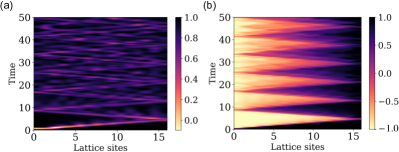
Figure 1: Spatiotemporal evolution of the ground state OTOC for (a) the JW local operator $\sigma^{z}$ and (b) the JW non-local operator $\sigma^{x}$, at the critical point of the TFIM given in Eq. (1) with $J_{x}=h=2$. The $\sigma^{z}$-OTOC shows only light-cone lines of information propagation, while the $\sigma^{x}$-OTOC shows alternating scrambling of quantum information and unscrambling after reflections from the ends.

Paramagnetic phase: spin-flip excitations. In the paramagnetic phase, at large values of the transverse field, $|h/J_{x}|\gg 1$, the ground state of the model has all the spins aligned in the direction of the field, $\ket{\uparrow\uparrow\uparrow\cdots\uparrow}_{z}$ in the $\sigma^{z}$-basis. The lowest energy excitations are given by single spin-flips like $\ket{\uparrow\downarrow\uparrow\cdots\uparrow}_{z}$. In the OTOC, $\sigma^{x}_{0}$ acting on the ground state creates a spin-flip excitation at the left-most (zero-th) site which can then hop through the chain due to the $J_{x}\sigma^{x}_{n}\sigma^{x}_{n+1}$ term in the Hamiltonian. Subsequently, $\sigma^{x}_{l}$ can either produce a second spin-flip excitation or de-excite the system back to the ground state. Thus, the ground state OTOC is approximately governed by a combination of two processes, one which involves only single spin-flip excitations and the other involving two spin-flips (see Fig. 2 (a)). This becomes clear if we write the OTOC using the intermediate excited states by resolving the identity approximately as $\mathbb{I}\approx\ket{\psi_{GS}}\bra{\psi_{GS}}+\sum_{q}\ket{q}\bra{q}+\sum_{q_{1},q_{2}}\ket{q_{1},q_{2}}\bra{q_{1},q_{2}}+$ higher order excitations.

$$F^{xx}(l,t)\simeq$$

$$\sum_{q,q^{\prime}}\big{[}\bra{\psi_{GS}}e^{iHt}\sigma^{x}_{l}\ket{q^{\prime}}\bra{q^{\prime}}e^{-iHt}\sigma^{x}_{0}\ket{\psi_{GS}}\bra{\psi_{GS}}e^{iHt}\sigma^{x}_{l}\ket{q}$$

$$\bra{q}e^{-iHt}\sigma^{x}_{0}\ket{\psi_{GS}}\big{]}+\sum_{q_{1},q_{4},q_{2}<q_{3}}\big{[}\bra{\psi_{GS}}e^{iHt}\sigma^{x}_{l}\ket{q_{4}}$$

$$\bra{q_{4}}e^{-iHt}\sigma^{x}_{0}\ket{q_{2},q_{3}}\bra{q_{2},q_{3}}e^{iHt}\sigma^{x}_{l}\ket{q_{1}}\bra{q_{1}}e^{-iHt}\sigma^{x}_{0}\ket{\psi_{GS}}\big{]},$$ (2)

where $\ket{q}$ and $\ket{q_{1},q_{2}}$ denote the eigenstates of the Hamiltonian with single and two spin-flip excitations, respectively. The quantum number $q$ takes the values $0,1,\dots,L-1$. It is worth noting that it is enough to consider processes up to the second order if $J_{x}/h$ is small. The matrix elements in Eq. (2) can be evaluated using the energies and wave functions of the excited states $\ket{q}$ and $\ket{q_{1},q_{2}}$. The single spin-flip excitations are described by an effective nearest-neighbour tight-binding model on the $L$-site lattice with open boundaries, and therefore have energies $\varepsilon_{q}=-2J_{x}~{}\cos(\frac{\pi q}{L+1})+2h$ above the ground state, and wave functions $\psi_{q}(n)=\braket{n}{q}=\sqrt{2/(L+1)}~{}\sin[\pi(q+1)(n+1)/(L+1)]$, where $\ket{n}=\sigma^{x}_{n}\ket{\psi_{GS}}$ denotes the state with a single flipped spin at site $n$.

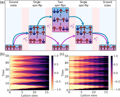
Figure 2: (a) Schematic of the mechanism of scrambling and unscrambling of $F^{xx}(l,t)$ involving two spin-flip excitations in the paramagnetic phase of the TFIM. (b) Spatiotemporal evolution of $F^{xx}(l,t)$ as obtained from a numerical time evolution for $J_{x}=2$ and $h=4$. (c) $F^{xx}(l,t)$ for the same parameter values obtained using the effective theory of two spin-flip excitations as mentioned in the text. The exact numerics and the effective theory calculations give remarkably similar results for the scrambling and unscrambling of $\sigma^{x}$.

While the single-particle eigenstates are solved by considering the problem of a particle in a box on a lattice, the case of two spin-flips is a bit subtle. The two spin-flips should be on separate sites and follow commutation relations, making it a system with two hard-core bosons. Due to the indistinguishability, we can write the wave function for two spin-flip excitations as $\psi_{q_{1},q_{2}}(n_{1},n_{2})=\braket{n_{1},n_{2}}{q_{1},q_{2}}=\psi_{q_{1}}(n_{1})\psi_{q_{2}}(n_{2})-\psi_{q_{2}}(n_{1})\psi_{q_{1}}(n_{2})$, where $\ket{n_{1},n_{2}}$ denotes the state with two spin-flips at sites $n_{1}$ and $n_{2}$, and we choose $n_{1}<n_{2}$. The energy this state is the sum of two single-particle energies, $\varepsilon_{q_{1},q_{2}}=\varepsilon_{q_{1}}+\varepsilon_{q_{2}}$. Finally, we arrive at SM

$$F^{xx}(l,t)\simeq\sum_{q,q^{\prime}}e^{-i(E_{q}+E_{q^{\prime}})t}\psi_{q}(l)\psi_{q}(0)\psi_{q^{\prime}}(l)\psi_{q^{\prime}}(0)$$

$$~{}+\sum_{q_{1},q_{4},q_{2}<q_{3}}e^{-i(E_{q_{1}}+E_{q_{4}}-E_{q_{2}}-E_{q_{3}})t}\psi_{q_{1}}(0)\psi_{q_{4}}(l)$$

$$\sum_{n_{1}}\psi_{q_{1}}(n_{1})\big{[}\theta(n_{1}-l)\psi_{q_{2},q_{3}}(l,n_{1})+\theta(l-n_{1})\psi_{q_{2},q_{3}}(n_{1},l)\big{]}$$

$$\sum_{n_{2}}\psi_{q_{4}}(n_{2})\psi_{q_{2},q_{3}}(0,n_{2}).$$ (3)

We evaluate this expression exactly and contrast the spatiotemporal evolution of $F^{xx}(l,t)$ calculated using exact numerical time-evolution with this analysis in Figs. 2 (b) and (c). The striking agreement confirms that spin-flip excitations indeed provide the mechanism responsible for the scrambling of quantum information and the unscrambling after a reflection when $h$ is large. Interestingly, this analysis agrees quite well with the exact result even if $h$ is not much larger than $J_{x}$. In fact, the plot for OTOC looks qualitatively the same for $h=J_{x}$ (Fig. 1 (b)) and $h>J_{x}$ (Fig. 2 (b)), although an analysis in terms of the spin-flip excitations cannot be assumed to be valid at the critical point.

Interactions in the presence of large field. We now look at the behavior of the OTOC in the PM phase in the presence of an integrability-breaking interaction term given by $J_{z}\sum_{n}\sigma^{z}_{n}\sigma^{z}_{n+1}$. The full Hamiltonian is given by $H=-J_{x}\sum_{n=0}^{L-2}\sigma^{x}_{n}\sigma^{x}_{n+1}-h\sum_{n=0}^{L-1}\sigma^{z}_{n}+J_{z}\sum_{n=0}^{L-2}\sigma^{z}_{n}\sigma^{z}_{n+1}$. When $|h/J_{x}|>1$, a small value of $J_{z}$ can significantly change the spatiotemporal plot for $F^{xx}(l,t)$, as shown in Fig. 3 (a). As usual, the local quantum information starts scrambling after $\sigma^{x}_{0}$ acts at one end. However, we do not see any unscrambling after reflection, unlike in the model without interactions. As time progresses further, the local information always stays scrambled and never becomes localized to a few sites. This can also be explained using a simple picture of two-spin flips. We need to modify Eq. (3) to account for two-spin flip states in the presence of interactions and evaluate it numerically. The wave functions for the two-spin flip state $\psi_{q_{1},q_{2}}(n_{1},n_{2})$ are replaced by two-body eigenstates calculated numerically by considering an effective tight-binding model with two hard-core bosons with a density-density interaction given by $J_{z}$. The OTOC calculated using this analysis involving only up to two-spin flips shows fairly good agreement with the plots obtained using exact numerics even with interactions. We contrast the two plots in Figs.  3 $(i)$ and $(ii)$ for the parameter values $J_{x}=2,~{}h=8$, and $J_{z}=1.8$.

We now introduce a simple space-time picture to understand the various spatiotemporal plots of the OTOC. We rewrite the expression for the OTOC as $F^{xx}(l,t)=\bra{\psi_{GS}}e^{iHt}\sigma^{x}_{l}e^{-iHt}\sigma^{x}_{0}e^{iHt}\sigma^{x}_{l}e^{-iHt}\sigma^{x}_{0}\ket{\psi_{GS}}=\braket{\psi_{2}}{\psi_{1}}$, where $\ket{\psi_{1}}$ and $\ket{\psi_{2}}$ are both states with one particle (spin-flip) and are defined respectively as $\ket{\psi_{1}}=\sigma^{x}_{0}e^{iHt}\sigma^{x}_{l}e^{-iHt}\sigma^{x}_{0}\ket{\psi_{GS}}$ and $\ket{\psi_{2}}=e^{iHt}\sigma^{x}_{l}e^{-iHt}\ket{\psi_{GS}}$. The state $\ket{\psi_{1}}$ can be interpreted as follows. Starting from the right, the first $\sigma^{x}_{0}$ operator creates a spin-flip at the end site which then propagates with some velocity for a time $t$ (due to $e^{-iHt}$). Next another spin-flip is created at site $l$. The two flipped spins then propagate back in time (due to $e^{iHt}$) to $t=0$ which involves zero, one or more scatterings between them depending on the position $l$ and time $t$. Finally, at $t=0$ one of the excitations is annihilated at site $l=0$ to produce a state with only one spin-flip. In contrast, $\ket{\psi_{2}}$ has a simpler interpretation as it involves a single spin-flip which is created at position $l$ and time $t$ on the time-evolved ground state, and which then propagates back in time to $t=0$. The inner product $\braket{\psi_{2}}{\psi_{1}}$ then depends on the scattering phase shift in the state $\ket{\psi_{1}}$ with respect to state $\ket{\psi_{2}}$.

Some assumptions are now required to estimate the value of the OTOC using scattering phase shifts. First, even though we are considering a system with open boundaries, we will assume that the system is large enough such that away from the edge, the momentum $q$ is a good quantum number. Second, we approximate a spin-flip excitation to be a quasiparticle with a single momenta $q_{0}$ with the largest velocity given by the Lieb-Robinson bound, although actually it is a superposition of many momentum states around $q_{0}$, propagating with the maximum possible group velocity. The entire region in the spatiotemporal plot of the OTOC can now be divided into regions according to the number of scatterings between the pair of quasiparticles with momenta $q_{0}$ and $-q_{0}$ in the state $\ket{\psi_{1}}$. The value of the OTOC (real part) in each region is approximately constant and is given by the real part of the scattering phase shift obtained from the two-particle Bethe ansatz SM .

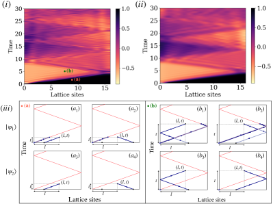
Figure 3: Spatiotemporal plots of $F^{xx}(l,t)$ for the interacting TFIM with $J_{x}=2,~{}h=8,~{}J_{z}=1.8$ obtained $(i)$ from exact numerics and $(ii)$ from the analysis using two spin-flip excitations. The value of $J_{z}$ is such that a region which showed scrambling in the non-interacting case now shows OTOC close to 1. $(iii)$ The point $(a)$ in the space-time plot corresponds to a region where there is no phase difference due to scattering between the states $\ket{\psi_{1}}$ and $\ket{\psi_{2}}$ (left panel), while at point $(b)$ (right panel) there is a scattering event between the two excitations in $\ket{\psi_{1}}$, and therefore the OTOC, defined as the inner product $\braket{\psi_{2}}{\psi_{1}}$ picks out the phase difference between the states.

The scrambling and unscrambling for the TFIM without interactions, given by the successive dark (OTOC close to $1$) and bright (OTOC close to $-1$), regions can be now understood as the regions having even and odd number of scatterings respectively starting from the lowest dark region with zero scattering. In the absence of interactions, every scattering event changes the phase by $e^{i\theta}=-1$. For the interacting model, the absence of unscrambling can be simply understood as the deviation of scattering phase shifts from $-1$ due to $J_{z}$. However, it should be noted that for later times the contributions from excitations not corresponding to the largest group velocity become significant and they alter the value of the OTOC obtained from the estimate given by scattering phase shift of two excitations.

To illustrate this, we have chosen two points $(a)$ and $(b)$ in the OTOC plots in Fig. 3 $(i)$ where point $(a)$ is in a region of no scrambling and $(b)$ is in a region of scrambling before any reflection. We now consider the schematic shown in Fig. 3 $(iii)$. The red lines are guides to the eye for the light-cone front. Then $\ket{\psi_{1}}$ at $(a)$ is given by a superposition of one-particle states shown in $(a_{1})$ and $(a_{2})$ with an intermediate process where a second excitation is first created at $(l,t)$ = $(0,0)$, then propagated forward in time, propagated back in time, and finally annihilated at the same point of creation. By contrast, $\ket{\psi_{2}}$ at $(a)$ is given by superposition of one-particle states shown in $(a_{3})$ and $(a_{4})$ without any other particles created or annihilated. Since there is no scattering event for point $(a)$, $F^{xx}=\braket{\psi_{2}}{\psi_{1}}=1$. Similarly, for point $(b)$, $\ket{\psi_{1}}$ is made of a superposition of states shown in $(b_{1})$ and $(b_{2})$ and $\ket{\psi_{2}}$ is made of a superposition of states shown in $(b_{3})$ and $(b_{4})$. In contrast to point $(a)$, we have one scattering phase shift between two excitations in the state $\ket{\psi_{1}}$ with respect to the state $\ket{\psi_{2}}$. Hence the inner product of the two states is given by the scattering phase shift which, for a pair of non-interacting hard-core bosons, is equal to $-1$; this explains the value of $F^{xx}(l,t)$ in the first scrambled region in the non-interacting TFIM. For the interacting case also it has a value close to $-1$. Subsequently, for larger times the scrambled and unscrambled regions have values of $F^{xx}(l,t)$ given by the total number of scattering events multiplied by the scattering phase shifts of one scattering event. In Figs. 3 $(i)$ and $(ii)$ we have considered a $J_{z}$ so that the region corresponding to three scattering events has $F^{xx}(l,t)$ close to $1$, which, for the non-interacting case, would have been close to $-1$.

The same effects are observed if we consider the integrable but interacting $XXZ$ spin-1/2 model in a transverse field. Namely, for the Hamiltonian, $H^{\prime}=-J\sum_{n=0}^{L-2}\sigma^{x}_{n}\sigma^{x}_{n+1}-J\sum_{n=0}^{L-2}\sigma^{y}_{n}\sigma^{y}_{n+1}-h\sum_{n=0}^{L-1}\sigma^{z}_{n}+J_{z}\sum_{n=0}^{L-2}\sigma^{z}_{n}\sigma^{z}_{n+1}$, the spatiotemporal plot for the OTOC shows a similar behavior including the absence of unscrambling as compared to the non-interacting $XX$ model without the $J_{z}$-term (see Fig. 6 in Ref. SM ). Therefore, a similar analysis in terms of the low-energy excitations holds true for the $XXZ$ spin-1/2 model also, implying that the absence of unscrambling is not related to the the integrability or non-integrability of the model.

Ferromagnetic phase: domain walls. We now discuss the scrambling in the FM phase of the TFIM. For very small $h$, the ground states are the degenerate states $\ket{I}=\ket{\uparrow\uparrow\cdots\uparrow}_{x}$ and $\ket{II}=\ket{\downarrow\downarrow\cdots\downarrow}_{x}$ in the $\sigma^{x}$-basis. The model has a $Z_{2}$ spin-flip symmetry, but the ground states spontaneously break it and the true ground states are the superpositions $\ket{+}=(\ket{I}+\ket{II})/\sqrt{2}$ and $\ket{-}=(\ket{I}-\ket{II})/\sqrt{2}$ corresponding to the even and odd fermion parity respectively. Setting $J_{x}=1$, and taking $h$ small, a perturbative expansion up to first order in $h$ SM yields the modified ground states expressed in a product form $\ket{I^{\prime}}=\ket{(\uparrow+\frac{h}{2}\downarrow)_{0}(\uparrow+\frac{h}{4}\downarrow)_{1}\cdots(\uparrow+\frac{h}{2}\downarrow)_{L-1}}_{x}$ and $\ket{II^{\prime}}=\ket{(\downarrow+\frac{h}{2}\uparrow)_{0}(\downarrow+\frac{h}{4}\uparrow)_{1}\cdots(\downarrow+\frac{h}{2}\uparrow)_{L-1}}_{x}$ (up to a normalization constant), where the subscripts denote the site indices. The lowest energy excitations are the two types of domain walls, namely $\ket{m+1/2,I}$ and $\ket{m+1/2,II}$, where the site label $m+\frac{1}{2}$ implies that the domain wall is situated between the $m$-th and $(m+1)$-th sites, and $I$ ($II$) denotes that all the spins on the left of the domain wall are down (up). Here $m$ can take values from $0$ to $L-2$. For example, $\ket{0+1/2,I}=\ket{\downarrow\uparrow\uparrow\cdots\uparrow}_{x}$ denotes the state with a domain wall between the first and second spins. Now, $\sigma^{x}_{0}$ acting on the state $\ket{I^{\prime}}$ creates the domain-wall state $\ket{0+1/2,I}$ with an amplitude $h$ to leading order. Under time evolution, this domain wall can move through the lattice with one less site due to the $h\sum\sigma^{z}_{n}$ term in the Hamiltonian, allowing us to construct domain-wall eigenstates with a quantum number label $\kappa$. Accordingly, domain-wall states have an energy dispersion $\epsilon_{\kappa,\alpha}=-2h$ sin$[\pi(\kappa+1)/L]+2J_{x}$ above the ground state, and a wave function $\phi_{\kappa,\alpha}(m)=\braket{m+1/2,\alpha\mid\kappa,\alpha}=\sqrt{2/L}~{}$sin$[\pi(\kappa+1)(m+1)/L]$, where $\kappa=0,1,\cdots,L-2$, and $\alpha$ can be $I$ or $II$. Subsequently, $\sigma^{x}_{l}$ for $l\neq 0$ does not create or destroy the domain-wall excitation but only measures if the spin is up or down in the $x$-basis. However, it changes the parity of the domain-wall excitation. The remaining $\sigma^{x}_{0}$ and $\sigma^{x}_{l}$ operators first de-excite the domain wall to a ground state with the opposite parity and then returns it to the ground state we started with. In short, as the domain moves from one end to the other end, it leaves flipped spins behind along its trajectory. This is then measured by the operator $\sigma^{x}_{l}$ at different times. The entire mechanism is described schematically in Fig. 4 (a). We have a different situation when $l=0$, as the four $\sigma^{x}_{0}$ operators sequentially excite and de-excite between the ground state and a domain-wall state, resulting in a different value of the OTOC at the edge.

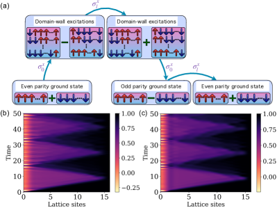
Figure 4: (a) Schematic of the mechanism of domain-wall assisted scrambling and unscrambling in the ordered phase of the TFIM. Spatiotemporal plots of $F^{xx}(l,t)$ for $J_{x}=2$ and $h=1$ obtained (b) using exact numerics in the ordered phase, and (c) using the analysis of domain-wall excitations described in the text. The remarkable agreement between these two plots suggests that indeed scrambling and unscrambling in the FM phase is governed by domain-wall excitations.

We now present a semi-analytical treatment of domain-wall dynamics to quantitatively understand scrambling and unscrambling. To this end, we construct the $\sigma^{x}$ operators at all sites which is perturbatively correct up to order $h$ in the subspace consisting only of the ground state and single domain-wall states. The operator $\sigma^{x}_{0}$ has non-trivial matrix elements only in the subspace of states $\{\ket{I^{\prime}},\ket{0+1/2,I}\}$ and $\{\ket{II^{\prime}},\ket{0+1/2,II}\}$. On the other hand, $\sigma^{x}_{L-1}$ has non-trivial elements in the subspaces spanned by the states $\{\ket{I^{\prime}},\ket{L-2+1/2,II}\}$ and $\{\ket{II^{\prime}},\ket{L-2+1/2,I}\}$. The $\sigma^{x}_{l}$ for all other sites are diagonal and have trivial matrix elements ($\pm 1$) up to order $h$ as they only determine whether the spin is up or down. The Hamiltonian then has a simple structure with only the ground state energy along the diagonal in the ground state basis and a tight-binding structure in the subspace of domain walls. Since the Hamiltonian only appears in the exponential in time evolution, we do not need to consider the matrix elements between the ground states and the domain walls to the lowest order.

The effective representations of $\sigma^{x}_{n}$ and the Hamiltonian $H$ in the subspace spanned by the set of states $\{\ket{I^{\prime}},\{\ket{m+1/2,I}\}_{m=0}^{L-2},\ket{II^{\prime}},\{\ket{m+1/2,II}\}_{m=0}^{L-2}\}$ are defined as $X_{n}$ and $\mathcal{H}$ (see Ref. SM for the explicit matrix forms). The OTOC in terms of domain-wall excitations can be written as

$$F^{xx}(l,t)\approx$$

$$\frac{1}{2}\bra{I^{\prime}+II^{\prime}}e^{i\mathcal{H}t}X_{l}e^{-i\mathcal{H}t}X_{0}e^{i\mathcal{H}t}X_{l}e^{-i\mathcal{H}t}X_{0}\ket{I^{\prime}+II^{\prime}}.$$ (4)

The plots for spatiotemporal evolution of $F^{xx}(l,t)$ using exact numerics and our analysis agree very well as shown in Figs. 4 (b) and (c). Moreover, in both the plots we observe the reflection of scrambled quantum information happening slightly before it reaches the other end, which validates that it is indeed governed by domain-wall excitations (which are defined midway between sites). The OTOC expression given in Eq. (4) is correct up to order $h^{2}$.

Interactions in the presence of small field. In the FM phase, the introduction of a small interaction $J_{z}$ (relative to $J_{x}$) in the Hamiltonian does not alter the qualitative features of the $F^{xx}(l,t)$ much. We can see scrambling and unscrambling much like the case without interactions in the spatiotemporal plots in OTOC. A small $J_{z}$ also gives rise to dynamics of a domain-wall by making it hop by two sites, in contrast to the transverse field $h$ which leads to hopping by one site. Therefore, the presence of a small interaction effectively only changes the dispersion of the domain walls to $E_{k}=-2h\cos k+2J_{z}\cos(2k)$. The group velocity is then given by $v_{k}=dE_{k}/dk=2h\sin k-4J_{z}\sin(2k)$. As the light-cone velocity is given by the maximum group velocity of the quasiparticles, for small $J_{z}/J_{x}$, the interacting model (Fig. 5 (a)) shows a different light-cone velocity than its non-interacting counterpart.

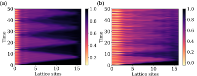
Figure 5: $F^{xx}(l,t)$ showing a pronounced unscrambling effect for (a) $J_{x}=2,~{}h=1,~{}J_{z}=0.5$, while for (b) $J_{x}=2,~{}h=1,~{}J_{z}=1$, it shows much less unscrambling. As $J_{z}$ becomes comparable to $J_{x}$ the perturbative expansion around the ground state becomes invalid. Also, higher order excitations become important and the scrambling is no longer due to single domain-wall motion.

If $J_{z}$ is increased further, we find that the unscrambling starts to go away. Roughly, this happens around $J_{z}/J_{x}\gtrsim 0.4$, as observed numerically. Fig.  5 (b) shows the absence of unscrambling for the parameter values $J_{x}=2,~{}h=1,~{}J_{z}=1$. It can be reasonably expected that for such values of $J_{z}$, the perturbative expansion starting from the states $\ket{I}$ and $\ket{II}$ will no longer be accurate. Furthermore, the assumption that only the lowest order excitations are responsible for information scrambling also becomes a gross oversimplification. To explain the absence of unscrambling when the interaction $J_{z}$ is comparable with $J_{x}$, one needs to account for higher order excitations like dynamics of three or more domain walls.

Conclusion. To summarize, we have studied the propagation of local quantum information in a spin-1/2 chain with open boundary conditions using ground state OTOCs of $\sigma^{z}$ and $\sigma^{x}$ operators which are local and non-local in terms of JW fermions respectively. While both $\sigma^{z}$ and $\sigma^{x}$ OTOCs show light-cone like propagation, only the $\sigma^{x}$ OTOC shows scrambling within the light-cone, in agreement with earlier results. In addition, we discover remarkable unscramblings and scramblings of the $\sigma^{x}$ OTOC after repeated reflections from the ends. We have provided, for the first time, an analytical understanding of both scrambling and unscrambling deep in the PM phase (when the transverse field $h$ is large) and the FM phase (when the $XX$ coupling $J_{x}$ is large) phases in terms of the low-energy excitations, namely, spin-flips when $h$ is large and domain walls when $J_{x}$ is large. When an interaction between JW fermions ($ZZ$ coupling) is added, the unscrambling effect becomes weaker. In the PM phase, even relatively weak interactions significantly change the scattering phase shift for two spin-flips and thereby reduces the unscrambling. In the FM phase, stronger interactions are required to destroy unscrambling and it occurs due the the creation of multiple domain wall excitations.

To conclude, we point out a recent experimental measurement of the OTOC Green et al. (2022) at finite temperature which, as the authors suggest, can also be performed for the ground state. In this paper, finite temperature OTOCs of the transverse field Ising model are studied for a trapped linear chain of ¹⁷¹Yb⁺ ions by creating a thermofield double state and then looking at its time evolution. We believe that a similar route can be followed to experimentally study the dynamics of low-energy excitations through the ground state OTOCs of the spin chains discussed in our work.

Acknowledgements. S.S. thanks MHRD, India for financial support through the PMRF. D.S. acknowledges funding from SERB, India (JBR/2020/000043).

I Supplemental Material

A: Derivation of expression for OTOC in Eq. (3)

We will present here the derivation of the final expression of the OTOC in terms of spin-flip excitations given in Eq. (3) for $|h/J_{x}|\gg 1$. The time evolution of the spin-flip eigenstates $e^{-iHt}\ket{q}$ and $e^{-iHt}\ket{q_{1},q_{2}}$ is trivial. The more difficult part is to find the matrix elements $\bra{q_{1},q_{2}}\sigma^{x}_{l}\ket{q}$. We use the resolution of identity,

$$\bra{q_{2},q_{3}}\sigma^{x}_{l}\ket{q_{1}}=\big{(}\frac{2}{L+1}\big{)}^{3/2}\sum_{n_{1},n_{2}<n3}\braket{q_{2},q_{3}}{n_{2},n_{3}}\braket{n_{2},n_{3}}{\sigma^{x}_{l}}{n_{1}}\braket{n_{1}}{q_{1}},$$ (S1)

and the wave functions $\braket{q_{2},q_{3}}{n_{2},n_{3}}=\psi_{q_{1},q_{3}}(n_{2},n_{3})$ and $\braket{n_{1}}{q_{1}}=\psi_{q}(n)$ as given in the main text. The matrix element $\braket{n_{2},n_{3}}{\sigma^{x}_{l}}{n_{1}}$ depends on whether $l<n_{1}$ or $l>n_{1}$ and we always choose $n_{2}<n_{3}$. Since $\sigma^{x}_{l}$ creates a spin-flip, we should have $l\neq n_{1}$. Therefore,

$$\braket{n_{2},n_{3}}{\sigma^{x}_{l}}{n_{1}}=\theta(n_{1}-l)\delta_{n_{2},l}\delta_{n_{1},n_{3}}+\theta(l-n_{1})\delta_{n_{3},l}\delta_{n_{1},n_{2}}.$$ (S2)

Using these relations we obtain Eq. (3) in the main text.

B: Perturbative ground state for $|h/J_{x}|<1$

k The degenerate ground states of the model in the limit of $h\to 0$ are $\ket{I}=\ket{\uparrow\uparrow\cdots\uparrow}_{x}$ and $\ket{II}=\ket{\downarrow\downarrow\cdots\downarrow}_{x}$. If a small $h$ is turned on, we obtain, from degenerate perturbation theory,

$$\ket{I^{\prime}} =\ket{I}+h\sum_{n}\frac{\ket{n}\braket{n}{\sum_{l}\sigma^{z}_{l}}{I}}{2(\delta_{n,0}+\delta_{n,N-1})+4(1-\delta_{n,0}-\delta_{n,N-1})}~{}+~{}O(h^{2})$$

$$=\ket{I}+\frac{h}{2}\ket{\downarrow\uparrow\uparrow\cdots}_{x}+\frac{h}{4}\ket{\uparrow\downarrow\uparrow\cdots}_{x}+\frac{h}{4}\ket{\uparrow\uparrow\downarrow\uparrow\cdots}_{x}+\cdots+\frac{h}{2}\ket{\uparrow\uparrow\cdots\downarrow}_{x},$$ (S3)

where $\ket{n}$ denotes the single spin-flip state in the $\sigma^{x}$-basis at site $n$. Combining these together we can write down the following perturbative ground state which is valid up to $O(h)$,

$$\ket{I^{\prime}}=\ket{(\uparrow+\frac{h}{2}\downarrow)_{0}(\uparrow+\frac{h}{4}\downarrow)_{1}\cdots(\uparrow+\frac{h}{2}\downarrow)_{L-1}}_{x}.$$ (S4)

In a similar way, we can derive the other perturbed ground state,

$$\ket{II^{\prime}}=\ket{(\downarrow+\frac{h}{2}\uparrow)_{0}(\downarrow+\frac{h}{4}\uparrow)_{1}\cdots(\downarrow+\frac{h}{2}\uparrow)_{L-1}}_{x}.$$ (S5)

C: Matrix forms for the operators in the domain-wall picture

We will derive here the matrix forms of the $\sigma^{x}$ operators in the ground state and the single domain-wall sector. We start with the $\sigma^{x}_{0}$ operator acting on the perturbed ground state $\ket{I^{\prime}}$, we will always make sure to consider processes which lie in low-energy sector and to work only up to $O(h)$.

$$\sigma^{x}_{0}\ket{I^{\prime}}=\ket{(\uparrow-\frac{h}{2}\downarrow)_{0}(\uparrow+\frac{h}{4}\downarrow)_{1}\cdots(\uparrow+\frac{h}{2}\downarrow)_{L-1}}_{x}=\ket{I^{\prime}}-h\ket{0+1/2,I}.$$ (S6)

We now consider the perturbed domain-wall state $\ket{0+1/2,I}$ up to an $O(h)$ correction. This can be written compactly as

$$\ket{0+1/2,I^{\prime}}=\ket{(\downarrow-\frac{h}{2}\uparrow)_{0}(\uparrow)_{1}(\uparrow+\frac{h}{4}\downarrow)_{2}\cdots(\uparrow+\frac{h}{2}\downarrow)_{L-1}}_{x}.$$ (S7)

Then the action of $\sigma^{x}_{0}$ on this state yields

$$\sigma^{x}_{0} \ket{0+1/2,I^{\prime}}=-\ket{(\downarrow)_{0}(\uparrow)_{1}(\uparrow+\frac{h}{4}\downarrow)_{2}\cdots(\uparrow+\frac{h}{2}\downarrow)_{L-1}}_{x}+h\ket{(\uparrow)_{0}(\uparrow+\frac{h}{4}\downarrow)_{1}\cdots(\uparrow+\frac{h}{2}\downarrow)_{L-1}}_{x}.$$ (S8)

Up to order $h$ we can simply write

$$\sigma^{x}_{0}\ket{0+1/2,I^{\prime}}=-\ket{0+1/2,I^{\prime}}+h\ket{I^{\prime}}.$$ (S9)

Therefore, in this small basis $\{\ket{I^{\prime}},\ket{0+1/2,I^{\prime}}\}$ the matrix form of $\sigma^{x}_{0}$ is given by

$$(X_{0})_{I}\approx\begin{pmatrix}\frac{1}{\sqrt{1+h^{2}}}&-\frac{h}{\sqrt{1+h^{2}}}\\ -\frac{h}{\sqrt{1+h^{2}}}&-\frac{1}{\sqrt{1+h^{2}}}\\ \end{pmatrix},$$ (S9)

where we have normalized the matrix to have $X_{0}^{2}=\mathbb{I}$ as it is an approximate representation of the unitary operator $\sigma^{x}_{0}$. Similarly, it can be shown that the effective normalized matrix form for the $\sigma^{x}_{0}$ operator in the basis $\{\ket{II^{\prime}},\ket{0+1/2,II^{\prime}}\}$ is given by,

$$(X_{0})_{II}\approx\begin{pmatrix}-\frac{1}{\sqrt{1+h^{2}}}&\frac{h}{\sqrt{1+h^{2}}}\\ \frac{h}{\sqrt{1+h^{2}}}&\frac{1}{\sqrt{1+h^{2}}}\\ \end{pmatrix}.$$ (S10)

On the rest of the domain-wall states, $\sigma^{x}_{0}$ does not produce any low-energy excitations up to $O(h)$. Therefore $\sigma^{x}_{0}$ only has diagonal matrix elements which can be expressed as

$$\braket{m+1/2,\alpha}{X_{0}}{m+1/2,\alpha}=(-1)^{\alpha},\text{for}~{}m>0.$$ (S11)

Here, $\alpha$ is equal to $I,II$ when it appears as a label in the domain-wall state and is equal to $1,2$ when it occurs in the power.

Combining all these, the $X_{0}$ matrix can be written as

$$X_{0} =\frac{1}{\sqrt{1+h^{2}}}\big{(}\outerproduct{I^{\prime}}{I^{\prime}}-h\outerproduct{I^{\prime}}{0+1/2,I}-h\outerproduct{0+1/2,I}{I^{\prime}}-\outerproduct{0+1/2,I}{0+1/2,I}\big{)}$$

$$~{}~{}~{}~{}-\frac{1}{\sqrt{1+h^{2}}}\big{(}\outerproduct{II^{\prime}}{II^{\prime}}-h\outerproduct{II^{\prime}}{0+1/2,II}-h\outerproduct{0+1/2,II}{II^{\prime}}-\outerproduct{0+1/2,II}{0+1/2,II}\big{)}$$

$$~{}~{}~{}~{}-\sum_{m=1}^{L-2}\outerproduct{m+1/2,I}{m+1/2,I}~{}+~{}\sum_{m=1}^{L-2}\outerproduct{m+1/2,II}{m+1/2,II}.$$ (S12)

The matrix form of the $\sigma^{x}_{L-1}$ operator at the other end can be derived in a similar fashion. The key thing is to note that $\sigma^{x}_{L-1}$ connects the pair of states $\ket{I^{\prime}}$ and $\ket{L-2+1/2,II}$ and also the pair $\{\ket{II^{\prime}},\ket{L-2+1/2,I}\}$. For the other domain-wall states, the matrix element of the operator is diagonal up to $O(h)$,

$$\braket{m+1/2,\alpha}{X_{L-1}}{m+1/2,\alpha}=(-1)^{\alpha+1}~{}~{}~{}\text{for}~{}~{}~{}0<m<L-1.$$ (S13)

Therefore the matrix representation of $\sigma^{x}_{L-1}$ in this low-energy sector is given by

$$X_{L-1} =\frac{1}{\sqrt{1+h^{2}}}\big{(}\outerproduct{I^{\prime}}{I^{\prime}}-h\outerproduct{I^{\prime}}{L-2+1/2,II}-h\outerproduct{L-2+1/2,II}{I^{\prime}}-\outerproduct{L-2+1/2,II}{L-2+1/2,II}\big{)}$$

$$~{}~{}~{}~{}-\frac{1}{\sqrt{1+h^{2}}}\big{(}\outerproduct{II^{\prime}}{II^{\prime}}-h\outerproduct{II^{\prime}}{L-2+1/2,I}-h\outerproduct{L-2+1/2,I}{II^{\prime}}-\outerproduct{L-2+1/2,I}{L-2+1/2,I}\big{)}$$

$$~{}~{}~{}~{}+\sum_{m=1}^{L-3}\outerproduct{m+1/2,I}{m+1/2,I}~{}-~{}\sum_{m=1}^{L-3}\outerproduct{m+1/2,II}{m+1/2,II}.$$ (S14)

The spin operators acting at sites other than the two ends do not produce or destroy a single domain wall. They can connect the ground state to states with two domain walls, but this is a higher order process and is therefore not considered in our analysis. Therefore, considering only the lowest energy excitations, the matrix elements of $\sigma^{x}_{l}$ for $l=1,\cdots,L-2$ are all diagonal. Hence they can be compactly represented as

$$X_{l}= \outerproduct{I^{\prime}}{I^{\prime}}-\outerproduct{II^{\prime}}{II^{\prime}}~{}+~{}\sum_{m=0}^{L-2}(\theta(l-m)+\theta(n-l+1))\outerproduct{m+1/2,I}{m+1/2,I}$$

$$~{}~{}-~{}\sum_{m=0}^{L-2}(\theta(l-m)+\theta(n-l+1))\outerproduct{m+1/2,II}{m+1/2,II}.$$ (S15)

D: Two-body scattering phase shift from the Bethe ansatz

We consider the Hamiltonian

$$H~{}=~{}\sum_{n=-\infty}^{\infty}~{}[-~{}J_{x}~{}\sigma^{x}_{n}\sigma^{x}_{n+1}~{}-~{}h~{}\sigma^{z}_{n}~{}+~{}J_{z}~{}\sigma^{z}_{n}\sigma^{z}_{n+1}],$$ (S16)

where we assume for simplicity that the system is infinitely long. For $h\gg J_{x},~{}J_{z}$, the ground state has all spins pointing up in the $\sigma^{z}$ basis. Let us call this the vacuum state $|{\rm vac}\rangle$. The lowest excited states are given by single spin-flip states where the spin at site $n$ points down while all the other spins point up. We will denote this state as $|n\rangle$, and it is related to the vacuum state as $|n\rangle=c_{n}^{\dagger}|{\rm vac}\rangle$. Here $c_{n}$ and $c_{n}^{\dagger}$ are annihilation and creation operators for hard-core bosons, since $(c_{n}^{\dagger})^{2}|{\rm vac}\rangle=0$. We note that $\sigma_{n}^{z}=1-2c_{n}^{\dagger}c_{n}$. In terms of these operators, the Hamiltonian can be written as

$$H_{c}~{}=~{}\sum_{n}~{}[2h~{}c_{n}^{\dagger}c_{n}~{}-~{}J_{x}~{}(c_{n}^{\dagger}c_{n+1}~{}+~{}c_{n+1}^{\dagger}c_{n})~{}+~{}4J_{z}~{}c_{n}^{\dagger}c_{n}c_{n+1}^{\dagger}c_{n+1}^{\dagger}],$$ (S17)

where we have ignored a constant equal to the ground state energy. We see that there is an interaction between spin-flip states on neighboring sites whose strength is given by $4J_{z}$.

The first excited states consist of single spin-flips. Considering a momentum eigenstate

$$|k\rangle~{}=~{}\sum_{n}~{}e^{ikn}~{}|n\rangle,$$ (S18)

we find from Eq. (S16) that the energy-momentum dispersion is $E_{k}=2h-2J_{x}\cos k$, where $k$ takes values in the range $[-\pi,\pi]$.

We now consider states consisting of two spin-flips. Defining such states as $|n_{1},n_{2}\rangle=c_{n_{1}}^{\dagger}c_{n_{2}}^{\dagger}|{\rm vac}\rangle$, where $n_{1}<n_{2}$, we consider a state with a wave function given by the Bethe ansatz

$$|k_{1},k_{2}\rangle~{}=~{}\sum_{n_{1}<n_{2}}~{}e^{i(k_{1}n_{1}+k_{2}n_{2})}+e^{i(\theta+k_{1}n_{2}+k_{2}n_{1})}~{}|n_{1},n_{2}\rangle.$$ (S19)

The momentum of this state is $k_{1}+k_{2}$ (since the wave function of the state $|n_{1}+1,n_{2}+1\rangle$ is $e^{i(k_{1}+k_{2})}$ times the wave function of $|n_{1},n_{2}\rangle$), and the energy is

$$E_{k_{1},k_{2}}~{}=~{}4h~{}-~{}2J_{x}~{}(\cos k_{1}~{}+~{}\cos k_{2}).$$ (S20)

The phase shift $\theta$ appearing in Eq. (S19) can be found in terms of $k_{1},~{}k_{2}$ by demanding that $H_{c}|k_{1},k_{2}\rangle=E_{k_{1},k_{2}}|k_{1},k_{2}\rangle$, and equating the coefficients of each real space state $|n_{1},n_{2}\rangle$ on the two sides of this equation. We discover that

$$e^{i\theta}~{}=~{}-~{}\frac{\cos(\frac{k_{1}+k_{2}}{2})~{}+~{}\frac{2J_{z}}{J_{x}}~{}e^{i(k_{2}-k_{1})/2}}{\cos(\frac{k_{1}+k_{2}}{2})~{}+~{}\frac{2J_{z}}{J_{x}}~{}e^{i(k_{1}-k_{2})/2}}.$$ (S21)

Note that in the absence of interactions, $J_{z}=0$, we get $e^{i\theta}=-1$ for all values of $k_{1},~{}k_{2}$.

In the main text, we are interested in the case where the two momenta $k_{1},~{}k_{2}$ are equal and opposite to each other. We therefore set $k_{1}=k_{0}$ and $k_{2}=-k_{0}$, where $k_{0}$ is determined by the condition that the single-particle group velocity $v_{k}=dE_{k}/dk$ is maximum as a function of $k$. The phase shift is then given by

$$e^{i\theta}~{}=~{}-~{}\frac{1~{}+~{}\frac{2J_{z}}{J_{x}}~{}e^{-ik_{0}}}{1~{}+~{}\frac{2J_{z}}{J_{x}}~{}e^{ik_{0}}}.$$ (S22)

E: Absence of unscrambling in $XXZ$ model and comparison with $XX$ model, both in a transverse field

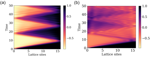
Figure 6: $F^{xx}(l,t)$ showing (a) scrambling and unscrambling for the $XX$ spin chain with parameters $J_{x}=J_{y}=1,~{}h=8,~{}J_{z}=0$, and (b) absence of unscrambling in the presence of interactions with the parameters $J_{x}=J_{y}=1,~{}h=8,~{}J_{z}=0.25$.

We present numerical results for $F^{xx}(l,t)$ for the non-interacting $XX$ spin-1/2 chain and the interacting but integrable $XXZ$ chain with a transverse field. Similar to the TFIM and the interacting non-integrable model discussed in the main text, this pair of models also show scrambling and unscrambling without interactions and absence of unscrambling with interactions. The plots shown in Fig. 6 correspond to the parameters, $(a)$ $J_{x}=J_{y}=1,~{}h=8,~{}J_{z}=0$, and $(b)$ $J_{x}=J_{y}=1,~{}h=8,~{}J_{z}=0.25$. We note that even such a small value of $J_{z}$ can completely destroy unscrambling as in the case discussed in the main text. This confirms that the absence of unscrambling is not due to non-integrability and can be simply explained by the scattering phase shift argument given in the main text.

References

- Roberts and Swingle (2016) D. A. Roberts and B. Swingle, Phys. Rev. Lett. 117, 091602 (2016).
- Hosur et al. (2016) P. Hosur, X.-L. Qi, D. A. Roberts, and B. Yoshida, Journal of High Energy Physics 2016, 1 (2016).
- Swingle and Chowdhury (2017) B. Swingle and D. Chowdhury, Phys. Rev. B 95, 060201 (2017).
- Patel et al. (2017) A. A. Patel, D. Chowdhury, S. Sachdev, and B. Swingle, Phys. Rev. X 7, 031047 (2017).
- Campisi and Goold (2017) M. Campisi and J. Goold, Phys. Rev. E 95, 062127 (2017).
- Iyoda and Sagawa (2018) E. Iyoda and T. Sagawa, Phys. Rev. A 97, 042330 (2018).
- Pappalardi et al. (2018) S. Pappalardi, A. Russomanno, B. Žunkovič, F. Iemini, A. Silva, and R. Fazio, Phys. Rev. B 98, 134303 (2018).
- Klug et al. (2018) M. J. Klug, M. S. Scheurer, and J. Schmalian, Phys. Rev. B 98, 045102 (2018).
- Kirkby et al. (2019) W. Kirkby, J. Mumford, and D. H. J. O’Dell, Phys. Rev. Res. 1, 033135 (2019).
- Alavirad and Lavasani (2019) Y. Alavirad and A. Lavasani, Phys. Rev. A 99, 043602 (2019).
- Sahu et al. (2019) S. Sahu, S. Xu, and B. Swingle, Phys. Rev. Lett. 123, 165902 (2019).
- Sur and Subrahmanyam (2022) S. Sur and V. Subrahmanyam, Quantum Information Processing 21, 301 (2022).
- Luitz and Bar Lev (2017) D. J. Luitz and Y. Bar Lev, Phys. Rev. B 96, 020406 (2017).
- Bohrdt et al. (2017) A. Bohrdt, C. B. Mendl, M. Endres, and M. Knap, New J. Phys. 19, 063001 (2017).
- Khemani et al. (2018) V. Khemani, A. Vishwanath, and D. A. Huse, Phys. Rev. X 8, 031057 (2018).
- Rakovszky et al. (2018) T. Rakovszky, F. Pollmann, and C. W. von Keyserlingk, Phys. Rev. X 8, 031058 (2018).
- Von Keyserlingk et al. (2018) C. Von Keyserlingk, T. Rakovszky, F. Pollmann, and S. L. Sondhi, Phys. Rev. X 8, 021013 (2018).
- Lieb and Robinson (1972) E. H. Lieb and D. W. Robinson, Comm. Math. Phys. 28, 251 (1972).
- Larkin and Ovchinnikov (1969) A. Larkin and Y. N. Ovchinnikov, JETP 28, 1200 (1969).
- Shenker and Stanford (2014) S. H. Shenker and D. Stanford, Journal of High Energy Physics 2014, 1 (2014).
- Maldacena et al. (2016) J. Maldacena, S. H. Shenker, and D. Stanford, Journal of High Energy Physics 2016, 1 (2016).
- Dóra and Moessner (2017) B. Dóra and R. Moessner, Phys. Rev. Lett. 119, 026802 (2017).
- Shen et al. (2017) H. Shen, P. Zhang, R. Fan, and H. Zhai, Phys. Rev. B 96, 054503 (2017).
- Heyl et al. (2018) M. Heyl, F. Pollmann, and B. Dóra, Phys. Rev. Lett. 121, 016801 (2018).
- Bao and Zhang (2020) J.-H. Bao and C.-Y. Zhang, Communications in Theoretical Physics 72, 085103 (2020).
- McGinley et al. (2019) M. McGinley, A. Nunnenkamp, and J. Knolle, Phys. Rev. Lett. 122, 020603 (2019).
- Riddell and Sørensen (2019) J. Riddell and E. S. Sørensen, Phys. Rev. B 99, 054205 (2019).
- Dağ et al. (2019) C. B. Dağ, K. Sun, and L.-M. Duan, Phys. Rev. Lett. 123, 140602 (2019).
- Zamani et al. (2022) S. Zamani, R. Jafari, and A. Langari, Phys. Rev. B 105, 094304 (2022).
- Shukla et al. (2021) R. K. Shukla, G. K. Naik, and S. K. Mishra, EPL 132, 47003 (2021).
- Suchsland et al. (2022) P. Suchsland, B. Douçot, K. Khemani, and R. Moessner, arXiv:2207.09502 (2022).
- Lin and Motrunich (2018) C.-J. Lin and O. I. Motrunich, Phys. Rev. B 97, 144304 (2018).
- Sur and Sen (2022) S. Sur and D. Sen, arXiv:2210.15302 (2022).
- Gopalakrishnan et al. (2018) S. Gopalakrishnan, D. A. Huse, V. Khemani, and R. Vasseur, Phys. Rev. B 98, 220303 (2018).
- Nahum et al. (2018) A. Nahum, S. Vijay, and J. Haah, Phys. Rev. X 8, 021014 (2018).
- Agrawal et al. (2019) U. Agrawal, S. Gopalakrishnan, and R. Vasseur, Phys. Rev. B 99, 174203 (2019).
- Lopez-Piqueres et al. (2021) J. Lopez-Piqueres, B. Ware, S. Gopalakrishnan, and R. Vasseur, Phys. Rev. B 104, 104307 (2021).
- Zhou et al. (2023) T. Zhou, A. Guo, S. Xu, X. Chen, and B. Swingle, Phys. Rev. B 107, 014201 (2023).
- (39) Supplemental Material .
- Green et al. (2022) A. M. Green, A. Elben, C. H. Alderete, L. K. Joshi, N. H. Nguyen, T. V. Zache, Y. Zhu, B. Sundar, and N. M. Linke, Phys. Rev. Lett. 128, 140601 (2022).