Robust Graph Matching Using An Unbalanced Hierarchical Optimal Transport Framework
Abstract
Graph matching is one of the most significant graph analytic tasks, which aims to find the node correspondence across different graphs. Most existing graph matching approaches mainly rely on topological information, whose performances are often sub-optimal and sensitive to data noise because of not fully leveraging the multi-modal information hidden in graphs, such as node attributes, subgraph structures, etc. In this study, we propose a novel and robust graph matching method based on an unbalanced hierarchical optimal transport (UHOT) framework, which, to our knowledge, makes the first attempt to exploit cross-modal alignment in graph matching. In principle, applying multi-layer message passing, we represent each graph as layer-wise node embeddings corresponding to different modalities. Given two graphs, we align their node embeddings within the same modality and across different modalities, respectively. Then, we infer the node correspondence by the weighted average of all the alignment results. This method is implemented as computing the UHOT distance between the two graphs — each alignment is achieved by a node-level optimal transport plan between two sets of node embeddings, and the weights of all alignment results correspond to an unbalanced modality-level optimal transport plan. Experiments on various graph matching tasks demonstrate the superiority and robustness of our method compared to state-of-the-art approaches. Our implementation is available at https://github.com/Dixin-Lab/UHOT-GM.
1 Introduction
Graph matching aims to find the node correspondence across different graphs, which commonly appears in many practical applications. For instance, protein-protein interaction (PPI) network alignment [34, 26] helps to explore the functionally-similar proteins of different species. Linking user accounts in different social networks benefits personalized recommendation [24, 25] and fraud detection [19, 18]. Vision tasks like shape matching can be formulated as graph matching problems [41, 11].
In practice, achieving exact graph matching is always challenging because of its NP-hardness. Therefore, many methods have been developed to match graphs approximately. Classic graph matching methods often formulate the task as a quadratic assignment problem (QAP) [27] based on graphs’ adjacency matrices [39, 21, 51] or other relation matrices [54, 16, 50, 46]. Recently, some learning-based graph matching methods [17, 38, 14] embed graph nodes and then align the node embeddings across different graphs. However, most existing methods merely apply specific information from a single modality (e.g., adjacency matrices, node attributes, or subgraph structures), leading to non-robust matching performance. Although some recent methods match graphs based on multi-modal information [37, 40], they often apply over-simplified mechanisms to fuse the multi-modal information, resulting in sub-optimal performance. To our knowledge, few existing graph matching approaches consider fully leveraging the multi-modal information hidden in graphs, let alone study the impacts of the cross-modal information on the matching results.
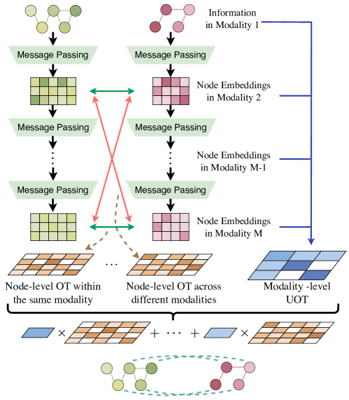
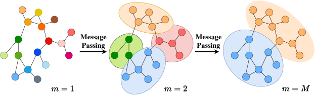
To overcome the above problems and fill in the blank, in this study we consider the multi-modal information of graphs and their interactions in graph matching tasks, proposing a robust graph matching method based on an unbalanced hierarchical optimal transport (UHOT) framework. As illustrated in Figure 1, our method formulates the graph matching task as an unbalanced hierarchical optimal transport problem. Given two graphs, we apply multi-layer message passing to generate their layer-wise node embeddings. The node embeddings obtained in each layer correspond to a modality, reflecting the structural information of the graphs at a specific smoothing strength. For the two graphs, we align their node embeddings within the same modality and across different modalities, respectively. Each alignment is achieved by computing the Gromov-Wasserstein (GW) distance [29] (or its variant [40]) between the corresponding node embedding sets, and the optimal transport (OT) plan associated with the distance indicates a node-level alignment result. Enumerating all modality pairs, we consider the weighted average of their corresponding OT plans as the graph matching result, in which the weights are learned by solving a modality-level unbalanced optimal transport (UOT) problem.
Solving the node-level and modality-level OT problems iteratively leads to the proposed UHOT framework, in which the node-level OT plans provide the alignment results based on different modalities’ information and the modality-level UOT plan determines the fusion mechanism of the alignment results. In the modality level, solving the UOT problem, in which the significance of different modalities is learned with regularization, helps avoid trivial solutions commonly in existing multi-modal graph matching methods [37] and thus improves the robustness of our method. We consider different implementations of the UHOT framework, including applying different OT distances [29, 40] and selecting different optimization algorithms [8] for the OT problems, and discuss the complexity and application scenarios of the implementations.
Different from existing graph matching methods, the proposed UHOT-based method, to our knowledge, first leverages the node alignment results across different modalities in an explicit way and demonstrates their contributions to improving final matching performance. It provides a new technical route seldom considered before for robust graph matching. We test our method in both synthetic and real-world graph matching tasks and compare it with state-of-the-art unsupervised and semi-supervised graph matching methods. Comprehensive experiments demonstrate the superiority of our method and its robustness.
2 Related Work
Optimal transport (OT) distance and its variants (like GW and FGW distances) provide an effective metric for probability measures (e.g., distributions). In particular, the OT distance in the Kantorovich form is called Wasserstein distance [20], which corresponds to computing an optimal transport plan between two probability measures. Given the samples of two probability measures, the optimal transport plan between them is formulated as a doubly stochastic matrix indicating the pairwise coherency of the samples [36, 29]. Because of this excellent property, OT distance has received great attention in extensive matching tasks, such as shape matching [35], generative modeling [15], and image-text alignment [4]. In graph analysis, OT distance is also gradually being adopted for graph-to-graph comparisons. Based on the GW distance, a series of OT-based graph matching methods have been proposed and achieved encouraging performance. GWL [46] is the first GW-based method that jointly learns the node embeddings and finds the node correspondence between two graphs. The FGW distance in [40] extends GW distance by considering the Wasserstein term for node attributes, so that it can be applied to match attribute graphs. SLOTAlign [37] combines GW distance with multi-view structure learning to enhance graph representation power and reduce the effect of structure and feature inconsistency inherited across graphs.
Recently, hierarchical optimal transport (HOT) [31, 1], as a generalization of original OT, is proposed to compare the distributions with structural information, e.g., measuring the distance between different Gaussian mixture models [5]. By solving OT plans at different levels, HOT has achieved encouraging performance in multi-modal distribution matching [23, 28], multi-modal learning [28], and neural architecture search [47]. To our knowledge, however, these HOT techniques have not yet been attempted in graph matching tasks. Additionally, unlike existing HOT work, our UHOT method leverages unbalanced optimal transport (UOT) at the modality-level. As demonstrated in [13, 6], compared to solving classic OT problems, solving UOT problems helps improve the robustness of domain adaptation [10] and generative modeling [48].
3 Proposed Method
3.1 Preliminaries and Motivation
In this study, we denote a graph as . Here, is the set of nodes. is the adjacency matrix, where denotes the presence of an edge between nodes and , and indicates the absence of an edge. denotes the node attribute matrix, where represents the number of nodes, and each node has an attribute vector . Given two graphs, i.e., and , graph matching aims to find the correspondence between their nodes. The node correspondence can be formulated as a matrix : for each , we can infer its correspondence in by . Without the loss of generality, in the following content, we assume that .
As aforementioned, classic graph matching methods often formulate the task as a QAP problem [27], i.e.,
| (1) |
where the correspondence matrix is formulated as a permutation matrix, and its feasible domain is denoted as . and are two relation matrices capturing the structural information of the two graphs, respectively. In practice, the relation matrices can be implemented as the adjacency matrices [39, 21, 51] (i.e., and ), the node similarity matrices [54, 3, 50] (i.e., and ), or their fusion results [16, 46].
When relaxing the correspondence matrix to a doubly stochastic matrix, i.e., , where and are two predefined node distributions that indicate the significance of nodes, we can reformulate the above QAP problem as computing a Gromov-Wasserstein (GW) distance between two graphs [29], i.e.,
| (2) |
where is the element of corresponding to the node pair in , and similarly, is the element of corresponding to the node pair in . The GW distance provides a valid distance metric for the collections of graphs [7]. In statistics, it computes the minimum expectation of the discrepancy of node pairs (i.e., the in equation 2). The doubly stochastic matrix corresponding to the minimum expectation, denoted as , is called the optimal transport (OT) plan, which can be viewed as a joint distribution of the nodes between the two graphs. Accordingly, the element in indicates the correspondence of the graphs’ nodes. Compared with the original QAP problem, the GW distance is much easier to compute [40, 46], making it a promising graph matching method.
The relation matrices, which contain the structural information of graphs, are crucial for the matching performance. Constructing the relation matrices purely based on a single modality (e.g., adjacency matrices or node attributes) often leads to non-robust matching results because the structural information of a single modality is sensitive to data noise [14, 37, 45, 21]. To overcome this robustness issue, some attempts have been made to leverage multi-modal information in graph matching tasks. Typically, the work in [40] proposes a variant of GW distance, called fused Gromov-Wasserstein (FGW) distance, considering the optimal transport based on both relation matrices and node attributes, i.e.,
| (3) |
where the first term is the Wasserstein term computing the expectation of the distance for node attribute pairs, and the second term is the GW term corresponding to the expectation in equation 2. The FGW distance aims to find the OT plan minimizing these two terms jointly, in which the hyperparameter controls their significance. When , the FGW distance degrades to the GW distance in equation 2, which matches two graphs based on a pair of relation matrices. Similarly, when , the FGW distance degrades to the Wasserstein distance [42] between node attributes.
Besides the FGW-based matching method, the SLOTAlign in [37] constructs the and in equation 2 by fusing multi-modal relation matrices linearly, i.e.,
| (4) |
Here, is the number of modalities, and is the relation matrix pair corresponding to the -th modality. is a learnable parameter vector defined in -Simplex, which determines the significance of the modalities. Typically, the relation matrices in different modalities are constructed based on different information, e.g., node attributes, adjacency matrices, and various graph kernels [2, 33, 32]. Given the and in equation 4, SLOTAlign matches graphs by computing their GW distance.
The above methods have demonstrated that multi-modal information indeed helps improve the robustness of graph matching. However, their over-simplified linear fusion mechanisms limit the utilization of the multi-modal information. In particular, the linear fusion step itself eliminates the identifiability of different modalities.111For example, merely based on the fused matrix in equation 4, we cannot obtain its multi-modal components . As a result, none of the existing methods consider the potential of matching graphs across different modalities, which may result in sub-optimal performance. In the following content, we propose a robust graph matching method using an unbalanced hierarchical optimal transport framework, which provides a new paradigm to leverage multi-modal information in graph matching tasks.
3.2 Proposed UHOT Framework
3.2.1 Multi-modal Information Extraction
In this study, we apply a set of non-learnable message passing layers to extract modalities’ information hidden in a graph. Typically, given a graph , we treat the initial node attribute matrix as the information of the first modality. The information of the -th modality is derived by passing through message passing layers as follows
| (5) |
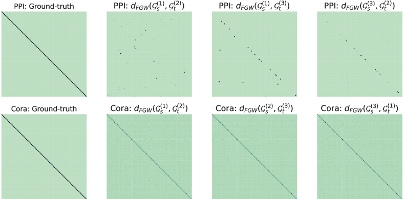
where is the symmetric normalized adjacency matrix with self-loop, is the identity matrix, and is the degree matrix of . From the perspective of graph spectral filtering, each message passing layer in equation 5 (i.e., ) works as a low-pass filter of the current node embeddings. With the increase in the number of message passing layers, the smoothness of the node embeddings increases accordingly. As a result, the node embeddings derived by different layers encode the structural information of the graph (e.g., the node clustering structure) in different granularity levels, as illustrated in Figure 2.
Denote the node embeddings of the modalities as a set . Inspired by SLOTAlign [37], we can further define a set of relational matrices for the graph, i.e., , where
| (6) |
As a result, we can reformulate a graph based on the above multi-modal information, denoted as , where each encodes the graph structural information of the -th modality.
3.2.2 Node-level Optimal Transports
Given two graphs with multi-modal information, i.e., and , we can align their nodes by computing their node-level optimal transport plans within each modality and across different modalities, respectively. In particular, we can construct a distance matrix with size , i.e., , where is the FGW distance between the graphs in the -th and -th modalities, respectively. We compute each by solving equation 3. An associated optimal transport plan is derived as . Following existing work [46, 44], we set the node distributions and to be uniform.
-
•
Remark 1. The OT plan indicates the node-level alignment results of the two graphs based on the -th and -th modalities, respectively. When , captures the node correspondence between and within the same modality. When , captures the node correspondence across different modalities. Different from existing methods, we enumerate all modality pairs and compute OT plans explicitly, i.e., , which explicitly considers the cross-modal alignment results.
3.2.3 A Modality-level Unbalanced Optimal Transport
For the two graphs, their modality pairs generally contribute to their matching with different significance. Therefore, given , we need to determine the weight of each automatically. In this study, we achieve this aim by solving an unbalanced optimal transport problem at the modality level. Specifically, taking the distance matrix as the grounding cost, we compute the minimum Wasserstein distance between two learnable modalities’ distributions, i.e.,
| (7) |
Here, are two learnable vectors in the -Simplex, indicating the significance of the modalities for and , respectively. is the set of the doubly-stochastic matrices that take and as marginals. is the transport matrix defined for the modalities. It can be explained as a joint distribution of the modalities corresponding to different graphs, and its element represents the coherency probability of the -th modality of and the -th modality of .
-
•
Remark 2. In principle, the matrix indicates the significance of different modality pairs. When the coherency probability of the modality pair (i.e., ) is large, the corresponding distance should be small, which means that and are matched well and their matching result is significant.
Note that, because and are learnable, the optimal solution of equation 7 may set them as one-hot vectors, so that only the associated with the minimum is one, while the remaining ’s are zeros. To avoid such a trivial solution, we further introduce a regularizer for and , penalizing their KL-divergence to the uniform distribution , i.e.,
| (8) |
Plugging equation 8 into equation 7 leads to the well-known unbalanced optimal transport (UOT) problem [13, 6].
3.2.4 Robust Graph Matching by Minimizing HOT
The composition of the above two-level optimal transport problems leads to a HOT distance between the graphs, i.e.,
| (9) |
where the grounding cost is constructed by the node-level FGW distances with the hyperparameter , and the Wasserstein distance computes the modality-level optimal transport plan. As a result, taking the regularizer in equation 8 into account, we can match two graphs by computing an unbalanced hierarchical optimal transport (UHOT) distance between them, i.e.,
| (10) |
This problem corresponds to the computation of the node-level optimal transport plans and the unbalanced modality-level optimal transport plan . We call this optimization problem “UHOT” because the marginals and are learnable variables regularized by the KL-divergence terms.
Given optimized and , we compute the final matching result as the weighted sum of all ’s, i.e.,
| (11) |
Accordingly, the final matching result is dominated by the ’s corresponding to the significant modality pairs.
3.3 Advantages Compared to Existing Methods
Our UHOT-based method provides a generalized framework for OT-based graph matching, and many existing methods can be viewed as its simplified special cases.
3.3.1 Compared to single-modal graph matching methods
As aforementioned, solving equation 10 without the regularizer leads to the following trivial solution
| (12) |
in which the optimal and are one-hot vectors, and their non-zero elements indicate the modality pair that corresponds to the minimum FGW distance. When , this trivial solution corresponds to matching and based on a single modality. When , only the original node attributes and adjacency matrices are applied to compute the FGW distance, and our UHOT-based method degrades to the single-modal strategy in [40]. When further setting , the FGW distance is specified as the GW distance, and our UHOT-based method is equivalent to the GWL method in [46, 45]. Introducing the regularizer in equation 8 allows us to effectively leverage the cross-modal alignment results (i.e., ).
3.3.2 Compared to multi-modal graph matching methods
As a representative multi-modal graph matching method, SLOTAlign [37] obtains an OT plan shared by all modality pairs by computing . It is easy to find that SLOTAlign can be treated as a special case of our UHOT-based method — when setting , the solution of SLOTAlign is also a feasible (non-optimal) solution of equation 10, i.e., , , and . In other words, SLOTAlign only considers the node-level alignment results within the same modality, and only the GW distance between each modality’s relation matrices is involved. Because of introducing the alignment results across different modalities and leveraging FGW distance, our UHOT-based method can be more robust than SLOTAlign. Additionally, although introducing a proximal gradient algorithm to update , SLOTAlign cannot prevent from being one-hot vector in theory because it does not consider the regularization of .
As another special case of our method, we can set , and the UHOT distance between graphs degrades to the classic HOT distance, i.e., . Furthermore, when we set and use GW distance as the grounding cost, we can prove that when is uniformly distributed,
| (13) |
In other words, when is uniformly distributed and , such a simplified UHOT distance provides a lower bound of SLOTAlign, given the scaling coefficient . Therefore, it is important for our method to optimize and explore significant modality pairs. The detailed proof is given in Appendix.
3.4 Optimization Algorithm
We propose a bi-level learning algorithm to solve the UHOT problem in equation 10. In this study, we apply the proximal gradient algorithm [45] or the conditional gradient (CG) algorithm [40] to compute each FGW distance efficiently. In theory, both of the algorithms ensure that the variables converge to a stationary point [46, 22]. Typically, for a graph with nodes and modalities, the computational complexity of the algorithms is . Fortunately, because the relation matrices we applied are constructed by the inner product of node embeddings, we can reduce the complexity of the algorithms to by leveraging the low-rank structures of the relation matrices [30].
In the modality-level, we need to compute the OT plan associated with the Wasserstein distance and update the marginals and . We achieve these two steps jointly in a Sinkhorn-based algorithmic framework. Specifically, we rewrite equation 7 by introducing an entropic regularizer, i.e.,
| (14) |
where , and is the hyperparameter controlling the importance of the entropy term. This entropic regularizer improves the smoothness of the original problem. Following existing work [8, 43, 28], the entropic OT problem in equation 14 can be solved efficiently by the Sinkhorn-scaling algorithm, whose computational complexity is . When updating the marginals, we apply the gradient descent algorithm [12], i.e.,
| (15) |
where is the learning rate. The gradients can be computed efficiently when applying the Sinkhorn-scaling iterations.
In summary, our method first computes distances and derives the corresponding optimal transport plans, each of which indicates a matching result for graph nodes. Then, the significance of the modalities is computed by solving an entropic OT problem with learnable marginals. The final matching result is obtained by aggregating all the matching plans according to equation 11. Algorithm 1 gives the pipeline of our method. The computational complexity of Algorithm 1 is , where is the number of outer loops and is the number of Sinkhorn-scaling iterations.
4 Experiments
4.1 Experimental Setup
Denote our UHOT-based graph matching method as UHOT-GM. We demonstrate its effectiveness by comparing it with state-of-the-art graph matching methods. Additionally, we provide comprehensive analytic experiments, verifying the rationality of using cross-modal alignment results and demonstrating the robustness of our method to data noise and hyperparameter settings. All the experiments are implemented in PyTorch and conducted on an NVIDIA 3090 GPU. Representative results are shown below. More implementation details and results are in Appendix.
| Dataset | #Nodes | #Edges | Dim. of Attr. |
| ACM-DBLP | 9,872 | 39,561 | 17 |
| 9,916 | 44,808 | 17 | |
| Douban Online-Offline | 3,906 | 16,328 | 538 |
| 1,128 | 3,022 | 538 | |
| Cora | 2,708 | 5,278 | 1,433 |
| PPI | 1,767 | 17,042 | 50 |
| Type | Method | ACM-DBLP | Douban Online-Offline | ||||
| NC@1 | NC@5 | NC@10 | NC@1 | NC@5 | NC@10 | ||
| semi- | IsoRank | 17.09 | 35.42 | 47.11 | 30.86 | 50.09 | 61.27 |
| supervised | FINAL | 30.25 | 55.32 | 67.95 | 52.24 | 89.80 | 95.97 |
| DeepLink | 12.19 | 32.98 | 44.58 | 8.86 | 22.36 | 30.95 | |
| CENALP | 34.81 | 51.86 | 62.23 | 23.70 | 38.10 | 43.56 | |
| unsupervised | UniAlign | 0.08 | 0.41 | 0.91 | 0.63 | 3.49 | 8.23 |
| REGAL | 3.49 | 9.74 | 13.61 | 1.97 | 6.44 | 10.11 | |
| GAlign | 58.43 | 78.78 | 84.46 | 44.10 | 67.98 | 77.73 | |
| WAlign | 63.91 | 83.86 | 89.12 | 39.53 | 61.63 | 71.02 | |
| GWL | 4.02 | 5.96 | 7.34 | 0.27 | 0.72 | 1.07 | |
| FGW | 49.11 | 52.06 | 52.09 | 58.86 | 63.23 | 63.69 | |
| SLOTAlign () | 65.52 | 84.05 | 87.76 | 49.91 | 74.69 | 79.43 | |
| UHOT-GM () | 67.65 | 85.26 | 88.52 | 54.03 | 67.71 | 70.93 | |
| UHOT-GM () | 69.53 | 86.97 | 90.26 | 62.97 | 71.47 | 75.76 | |
| UHOT-GM () | 70.13 | 87.19 | 90.86 | 59.93 | 74.06 | 77.28 | |
| Type | Method | PPI | Cora | ||||
| NC@1 | NC@5 | NC@10 | NC@1 | NC@5 | NC@10 | ||
| semi- | IsoRank | 17.71 | 28.64 | 34.75 | 16.88 | 34.12 | 42.95 |
| supervised | FINAL | 38.09 | 52.91 | 55.35 | 67.25 | 81.35 | 85.52 |
| DeepLink | 10.36 | 14.94 | 18.05 | 10.86 | 27.81 | 36.34 | |
| CENALP | 28.35 | 41.43 | 47.82 | 76.55 | 86.85 | 88.81 | |
| unsupervised | UniAlign | 0.68 | 2.77 | 4.92 | 0.41 | 1.85 | 3.91 |
| REGAL | 6.68 | 18.11 | 25.69 | 5.50 | 11.11 | 14.73 | |
| GAlign | 67.18 | 78.49 | 82.57 | 98.38 | 99.85 | 99.96 | |
| WAlign | 64.63 | 73.23 | 76.91 | 93.72 | 96.01 | 96.38 | |
| GWL | 11.38 | 13.30 | 16.07 | 0.03 | 0.11 | 0.37 | |
| FGW | 83.32 | 83.32 | 83.32 | 99.19 | 99.19 | 99.19 | |
| SLOTAlign () | 76.63 | 82.06 | 83.76 | 98.86 | 99.89 | 99.89 | |
| UHOT-GM () | 86.64 | 90.89 | 92.30 | 99.45 | 100.00 | 100.00 | |
| UHOT-GM () | 87.10 | 91.06 | 92.13 | 99.41 | 100.00 | 100.00 | |
| UHOT-GM () | 83.93 | 89.64 | 91.17 | 99.45 | 100.00 | 100.00 | |
4.1.1 Datasets
In this study, we consider four graph datasets. Each dataset contains one or two real-world graphs with their topology and attribute information. Table 1 shows the statistics of the datasets. Details for datasets are described below.
-
•
ACM-DBLP [52] is a two co-authorship networks dataset for publication information. The ACM network includes 9,916 authors (i.e., nodes) and 44,808 co-authorships (i.e., edges), while the DBLP network includes 9,872 authors and 39,561 co-authorships. Node attributes are composed of the number of papers published by the author in 17 locations. The 6,325 co-authors in the two networks constitute the ground-truth node correspondence.
-
•
Douban Online-Offline [53] includes an online graph with 16,328 interactions among 3,906 users and an offline graph with 3,022 interactions among 1,118 users. The user’s location represents node attributes. The ground-truth node correspondence is the 1,118 users appearing in both graphs.
-
•
Cora [49] is a citation network, whose nodes are publications and edges are citation relations. It has 2,708 nodes and 5,278 edges, and each node has 1,433 attributes.
-
•
PPI [56] is a protein-protein interaction network. It contains 1,767 nodes with 50 attributes and 17,042 edges.
Since Cora and PPI only contain one graph, we generate the other graph by cutting % edges in the original graph randomly and adding % random edges accordingly. Here, , indicating different noise levels.
4.1.2 Baselines
For each dataset, we select seven unsupervised graph matching methods as baselines. Among them, UniAlign [21] is based on solving a QAP problem, REGAL [17], WAlign [14], and GAlign [38] are based on node embedding alignment, and GWL [46], FGW [40], and SLOTAlign [37] are based on computing OT distances. Furthermore, to demonstrate the advantages of UHOT-GM as an unsupervised method, we select four semi-supervised baselines for comparison, including IsoRank [34], FINAL [52], DeepLink [55] and CENALP [9]. These semi-supervised baselines require partial node pairs as training labels. We use 10% of the ground-truth node pairs when implementing these semi-supervised methods.
4.1.3 Hyperparameter Setting.
Our UHOT-GM applies three message passing layers to generate four modalities, leading to a fair comparison with SLOTAlign. Additionally, to demonstrate the efficiency of UHOT-GM in using multi-modal information, we also apply UHOT-GM with two or three modalities, respectively. By default, we apply FGW distance in UHOT-GM and compute it by the proximal gradient algorithm [46], with . When solving the modality-level UOT problem, we set the weight of the entropic regularizer in equation 14 as and the learning rate of the modality distributions as . The robustness of our method to the hyperparameters is shown in the following analytic experiments.
4.1.4 Metrics
For each method, we evaluate its performance by the commonly used Top-K node correctness (denoted as NC@K). In particular, given a node of the graph , NC@K takes the most similar nodes from all possible matching in the graph as a Top-K list, and finally calculates the percentage of ground-truth matching in the list. Note that, since we implement semi-supervised baselines with 10% of the ground-truth, we take the ground-truth into account in the final results as well so that we can compare them fairly with unsupervised methods. For each dataset, we implement each method five times with different random seeds and report its average performance in the five trials.
4.2 Numerical Comparisons
4.2.1 Node Correctness
Table 2 shows the matching performance of various methods on the four datasets. We can find that UHOT-GM achieves the best NC@1 results on all four datasets, which even outperforms those semi-supervised baselines. In particular, the performance of some unsupervised methods, like IsoRank, UniAlign, REGAL, and GWL, is unsatisfactory because they merely leverage the graph topological information (i.e., adjacency matrices) to match graphs while ignoring the utilization of other modalities (e.g., node attributes and subgraph structures). On the contrary, the methods applying multi-modal information, including UHOT-GM, often achieve encouraging results. This phenomenon demonstrates the usefulness of multi-modal information in graph matching tasks.
UHOT-GM performs consistently better than others on ACM-DBLP, PPI, and Cora. For the most challenging Douban Online-Offline dataset, where there exists a large disparity in the number of nodes, UHOT-GM still performs the best on NC@1 and achieves comparable results on NC@5 and NC@10. This result shows that UHOT-GM remains competitive in those graph matching tasks with extremely imbalanced nodes. Additionally, the most competitive multi-modal baseline, SLOTAlign, applies four modalities, while the UHOT-GM using three modalities can overcome its performance on NC@1. This phenomenon implies that compared to SLOTAlign, UHOT-GM can leverage multi-modal information of graphs more effectively, and taking cross-modal alignment results into account indeed contributes to improved matching performance.
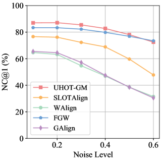
4.2.2 Robustness to Noise
Given the PPI graphs, whose ratio of randomly reconnected edges increases from to , we test various unsupervised graph matching methods on their robustness to data noise. Experimental results in Figure 3(a) show that the methods using FGW distance, e.g., FGW and our UHOT-GM, maintain high node correctness even if 60% of edges are affected by noise. On the contrary, SLOTAlign and WAlign consider the GW and Wasserstein distances between graphs, respectively, whose performance is sensitive to noise. These results indicate that in highly-noisy matching tasks, applying FGW distance, which computes the OT plan based on both node embeddings and relation matrices, helps improve the robustness of the OT-based matching methods.
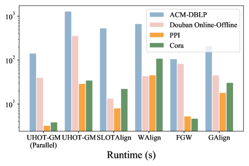
4.2.3 Runtime Comparison
Figure 3(b) shows the comparison for various unsupervised graph matching methods on runtime. We can find that the runtime of UHOT-GM is comparable to that of WAlign and GAlign. Compared to FGW and SLOTAlign, UHOT-GM takes longer time in general because it computes multiple FGW distances. Taking the improvement in node correctness into account, we think the computational complexity of UHOT-GM is tolerable. Moreover, the FGW distances involved in UHOT-GM can be computed in parallel, so the runtime of UHOT-GM in practice can be comparable to that of FGW and SLOTAlign as well, as shown in the “UHOT-GM (Parallel)” group of Figure 3(b).
| Used | ACM-DBLP | Douban Online-Offline | ||||
| Modalities | NC@1 | NC@5 | NC@10 | NC@1 | NC@5 | NC@10 |
| Proposed | 70.13 | 87.19 | 90.86 | 59.93 | 74.06 | 77.28 |
| Only Low-pass | 40.76 | 60.40 | 67.98 | 10.91 | 26.39 | 27.28 |
| Add High-pass | 68.57 | 85.82 | 90.03 | 35.51 | 72.81 | 76.74 |
4.3 Ablation Study
4.3.1 The Rationality of Proposed Message Passing
The message passing layers used in UHOT-GM work as low-pass graph filters. They extract graph structural information in different granularity levels. In general, these low-pass modalities are insensitive to the noise imposed on graphs. As a result, UHOT-GM leverages these low-pass modalities jointly with the original graph structural information (i.e., node attributes and adjacency matrices) to achieve graph matching robustly. Here, two questions arise: Can we achieve robust graph matching purely based on the low-pass modalities? Can high-pass modalities lead to robust graph matching? To answer these two questions, we consider two variants of the proposed message passing mechanism. In particular, “Only Low-pass” means that we only apply the last two layers’ embeddings (i.e., the low-pass modalities) as the multi-modal information to match graphs. “Add High-pass” means that besides the original modalities, we further take the high-pass graph filtering result, i.e., , where is normalized graph Laplacian matrix, as an additional modality and match graphs accordingly.
Table 3 shows the graph matching results achieved by the UHOT-GM using different message-passing mechanisms. We can find that the proposed message-passing mechanism achieves the best performance, while the above two variants lead to performance degradation. Firstly, when only considering the low-pass modalities, we lose the information on original node attributes and adjacency matrices, which harms the matching results. Secondly, applying the high-pass modality to graph matching tasks may be inappropriate. In particular, graph matching is naturally sensitive to the topological noise (e.g., the random connections and disconnections of edges) in graphs [38, 37], while the high-pass graph filtering encodes the discrepancy of node attributes along graph edges, whose output is largely influenced by the noise of the edges. In summary, the results in Table 3 demonstrate the rationality of our method.
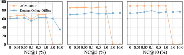
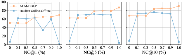
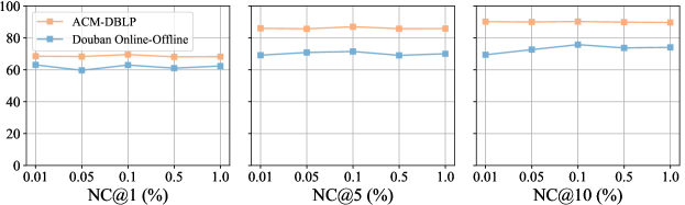
4.3.2 The Robustness to Key Hyperparameters
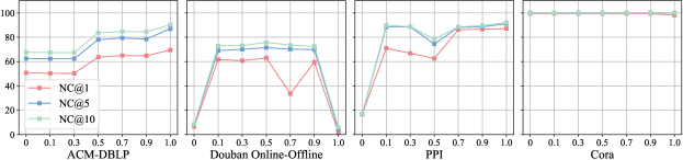
Our UHOT-GM method has three key hyperparameters, including the learning rate of modalities’ significance, the weight in FGW distance, and the weight of the KL-divergence regularizer. Taking the learning rate from , we explore its impact on matching results in Figure 4(a). In particular, when , it means that we fix , treating each modality evenly. When , we update and iteratively, with the corresponding learning rate. The results in Figure 4(a) show that the UHOT-GM is robust to in a wide range (i.e., ), and the best performance is achieved when . When the learning rate is too large, the update of and becomes too aggressive and leads to undesired results. In Figure 4(b), we explore the impact of on the matching results of two datasets. We can find that when , the NC@5 and NC@10 of UHOT-GM are relatively stable, which demonstrates the robustness of UHOT-GM to . Based on the results in Figure 4(b), we can set robustly in practice. Similarly, UHOT-GM is also robust to the weight in the range , as shown in Figure 4(c).
4.3.3 The Rationality of Cross-modal Alignment
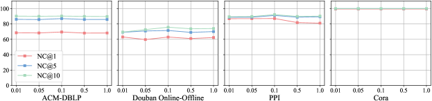
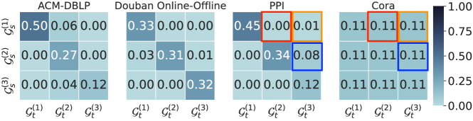
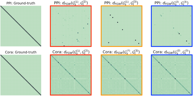
In Figure 5(a), we visualize the modality-level OT plans obtained by UHOT-GM for different datasets. The OT plans of ACM-DBLP and Douban Online-Offline are diagonally-dominant, which means that their matching results are mainly based on the node-level alignment within the same modality. However, for PPI and Cora, the contributions of cross-modal alignment results become significant. For PPI, the upper triangle part of its modality-level OT plan has a significant value. For Cora, its modality-level OT plan is close to a uniform distribution, which means that the node-level alignment within the same modality and those across different modalities contribute evenly to the final matching results.
We further mark the upper triangle elements in the modality-level OT plans of PPI and Cora (i.e., the color boxes in Figure 5(a)). Each mark corresponds to a modality pair, and we visualize the corresponding node-level OT plans in Figure 5(b). We can find that for those insignificant modality pairs (e.g., and for PPI), their node-level OT plans are distinguished from the ground truth node correspondence. On the contrary, for those significant modality pairs (e.g., those for Cora), their node-level OT plans are similar to the ground truth node correspondence. These phenomena demonstrate the rationality of our method — UHOT-GM can find useful cross-modal alignment results and assign them large weights when inferring node correspondence.
5 Conclusion and Future Work
In this work, we propose a novel UHOT framework for graph matching, leveraging multi-modal information of graphs to achieve robust matching results. The proposed UHOT framework makes the first attempt to leverage the cross-modal alignment results explicitly in graph matching tasks, and it avoids trivial solutions by considering the unbalanced modality-level optimal transport. Experimental results show that the UHOT-based method achieves encouraging performance in unsupervised graph matching tasks and even outperforms those semi-supervised learning methods. In summary, our work demonstrates the usefulness of OT-based cross-modal alignment in graph matching tasks, which points out a new technical route seldom considered before. In the future, we plan to extend the proposed method, applying it to match more complicated graph structures, e.g., hierarchical graphs and hypergraphs. At the same time, we would like to introduce stochastic optimization strategies to improve the efficiency of our algorithm.
References
- [1] D. Alvarez-Melis, T. S. Jaakkola, and S. Jegelka. Structured optimal transport. In International Conference on Artificial Intelligence and Statistics, AISTATS 2018, 9-11 April 2018, Playa Blanca, Lanzarote, Canary Islands, Spain, volume 84, pages 1771–1780. PMLR, 2018.
- [2] K. M. Borgwardt and H. Kriegel. Shortest-path kernels on graphs. In Proceedings of the 5th IEEE International Conference on Data Mining (ICDM 2005), 27-30 November 2005, Houston, Texas, USA, pages 74–81. IEEE Computer Society, 2005.
- [3] T. S. Caetano, J. J. McAuley, L. Cheng, Q. V. Le, and A. J. Smola. Learning graph matching. IEEE transactions on pattern analysis and machine intelligence, 31(6):1048–1058, 2009.
- [4] L. Chen, Z. Gan, Y. Cheng, L. Li, L. Carin, and J. Liu. Graph optimal transport for cross-domain alignment. In Proc. of ICML, volume 119, pages 1542–1553. PMLR, 2020.
- [5] Y. Chen, T. T. Georgiou, and A. Tannenbaum. Optimal transport for gaussian mixture models. IEEE Access, 2018.
- [6] L. Chizat, G. Peyré, B. Schmitzer, and F. Vialard. Scaling algorithms for unbalanced optimal transport problems. Math. Comput., 87(314):2563–2609, 2018.
- [7] S. Chowdhury and F. Mémoli. The gromov–wasserstein distance between networks and stable network invariants. Information and Inference: A Journal of the IMA, 8(4):757–787, 2019.
- [8] M. Cuturi. Sinkhorn distances: Lightspeed computation of optimal transport. In Advances in Neural Information Processing Systems 26: 27th Annual Conference on Neural Information Processing Systems 2013. Proceedings of a meeting held December 5-8, 2013, Lake Tahoe, Nevada, United States, pages 2292–2300, 2013.
- [9] X. Du, J. Yan, and H. Zha. Joint link prediction and network alignment via cross-graph embedding. In Proceedings of the Twenty-Eighth International Joint Conference on Artificial Intelligence, IJCAI 2019, Macao, China, August 10-16, 2019, pages 2251–2257. ijcai.org, 2019.
- [10] K. Fatras, T. Séjourné, R. Flamary, and N. Courty. Unbalanced minibatch optimal transport; applications to domain adaptation. In Proceedings of the 38th International Conference on Machine Learning, ICML 2021, 18-24 July 2021, Virtual Event, volume 139, pages 3186–3197. PMLR, 2021.
- [11] M. Fey, J. E. Lenssen, C. Morris, J. Masci, and N. M. Kriege. Deep graph matching consensus. In Proc. of ICLR. OpenReview.net, 2020.
- [12] C. Frogner, C. Zhang, H. Mobahi, M. Araya, and T. A. Poggio. Learning with a wasserstein loss. Advances in neural information processing systems, 28, 2015.
- [13] C. Frogner, C. Zhang, H. Mobahi, M. Araya-Polo, and T. A. Poggio. Learning with a wasserstein loss. In Advances in Neural Information Processing Systems 28: Annual Conference on Neural Information Processing Systems 2015, December 7-12, 2015, Montreal, Quebec, Canada, pages 2053–2061, 2015.
- [14] J. Gao, X. Huang, and J. Li. Unsupervised graph alignment with wasserstein distance discriminator. In Proceedings of the 27th ACM SIGKDD Conference on Knowledge Discovery & Data Mining, 2021.
- [15] A. Genevay, G. Peyré, and M. Cuturi. Learning generative models with sinkhorn divergences. In International Conference on Artificial Intelligence and Statistics, AISTATS 2018, 9-11 April 2018, Playa Blanca, Lanzarote, Canary Islands, Spain, volume 84, pages 1608–1617. PMLR, 2018.
- [16] S. Hashemifar, Q. Huang, and J. Xu. Joint alignment of multiple protein–protein interaction networks via convex optimization. Journal of Computational Biology, (11), 2016.
- [17] M. Heimann, H. Shen, T. Safavi, and D. Koutra. REGAL: representation learning-based graph alignment. In Proceedings of the 27th ACM International Conference on Information and Knowledge Management, CIKM 2018, Torino, Italy, October 22-26, 2018, pages 117–126. ACM, 2018.
- [18] B. Hooi, K. Shin, H. A. Song, A. Beutel, N. Shah, and C. Faloutsos. Graph-based fraud detection in the face of camouflage. ACM Transactions on Knowledge Discovery from Data (TKDD), (4), 2017.
- [19] M. Huang, Y. Liu, X. Ao, K. Li, J. Chi, J. Feng, H. Yang, and Q. He. Auc-oriented graph neural network for fraud detection. In Proceedings of the ACM Web Conference 2022, 2022.
- [20] L. V. Kantorovich. On the translocation of masses. In Dokl. Akad. Nauk. USSR (NS), 1942.
- [21] D. Koutra, H. Tong, and D. Lubensky. Big-align: Fast bipartite graph alignment. In 2013 IEEE 13th international conference on data mining. IEEE, 2013.
- [22] S. Lacoste-Julien. Convergence rate of frank-wolfe for non-convex objectives. CoRR, abs/1607.00345, 2016.
- [23] J. Lee, M. Dabagia, E. L. Dyer, and C. Rozell. Hierarchical optimal transport for multimodal distribution alignment. In Advances in Neural Information Processing Systems 32: Annual Conference on Neural Information Processing Systems 2019, NeurIPS 2019, December 8-14, 2019, Vancouver, BC, Canada, pages 13453–13463, 2019.
- [24] C. Li, S. Wang, H. Wang, Y. Liang, P. S. Yu, Z. Li, and W. Wang. Partially shared adversarial learning for semi-supervised multi-platform user identity linkage. In Proceedings of the 28th ACM International Conference on Information and Knowledge Management, CIKM 2019, Beijing, China, November 3-7, 2019, pages 249–258. ACM, 2019.
- [25] C. Li, S. Wang, P. S. Yu, L. Zheng, X. Zhang, Z. Li, and Y. Liang. Distribution distance minimization for unsupervised user identity linkage. In Proceedings of the 27th ACM International Conference on Information and Knowledge Management, CIKM 2018, Torino, Italy, October 22-26, 2018, pages 447–456. ACM, 2018.
- [26] Y. Liu, H. Ding, D. Chen, and J. Xu. Novel geometric approach for global alignment of PPI networks. In Proc. of AAAI, pages 31–37. AAAI Press, 2017.
- [27] E. M. Loiola, N. M. M. De Abreu, P. O. Boaventura-Netto, P. Hahn, and T. Querido. A survey for the quadratic assignment problem. European journal of operational research, (2), 2007.
- [28] D. Luo, H. Xu, and L. Carin. Differentiable hierarchical optimal transport for robust multi-view learning. IEEE Transactions on Pattern Analysis and Machine Intelligence, 2022.
- [29] F. Mémoli. Gromov–wasserstein distances and the metric approach to object matching. Foundations of computational mathematics, 2011.
- [30] M. Scetbon, G. Peyré, and M. Cuturi. Linear-time gromov wasserstein distances using low rank couplings and costs. In International Conference on Machine Learning, ICML 2022, 17-23 July 2022, Baltimore, Maryland, USA, volume 162, pages 19347–19365. PMLR, 2022.
- [31] B. Schmitzer and C. Schnörr. A hierarchical approach to optimal transport. In International conference on scale space and variational methods in computer vision. Springer, 2013.
- [32] N. Shervashidze, P. Schweitzer, E. J. van Leeuwen, K. Mehlhorn, and K. M. Borgwardt. Weisfeiler-lehman graph kernels. J. Mach. Learn. Res., 12:2539–2561, 2011.
- [33] N. Shervashidze, S. V. N. Vishwanathan, T. Petri, K. Mehlhorn, and K. M. Borgwardt. Efficient graphlet kernels for large graph comparison. In Proceedings of the Twelfth International Conference on Artificial Intelligence and Statistics, AISTATS 2009, Clearwater Beach, Florida, USA, April 16-18, 2009, volume 5, pages 488–495. JMLR.org, 2009.
- [34] R. Singh, J. Xu, and B. Berger. Global alignment of multiple protein interaction networks with application to functional orthology detection. Proceedings of the National Academy of Sciences, (35), 2008.
- [35] J. Solomon, G. Peyré, V. G. Kim, and S. Sra. Entropic metric alignment for correspondence problems. ACM Transactions on Graphics (ToG), (4), 2016.
- [36] B. Su and G. Hua. Order-preserving wasserstein distance for sequence matching. In 2017 IEEE Conference on Computer Vision and Pattern Recognition, CVPR 2017, Honolulu, HI, USA, July 21-26, 2017, pages 2906–2914. IEEE Computer Society, 2017.
- [37] J. Tang, W. Zhang, J. Li, K. Zhao, F. Tsung, and J. Li. Robust attributed graph alignment via joint structure learning and optimal transport. In Proc. of ICDE, pages 1638–1651. IEEE, 2023.
- [38] H. T. Trung, T. Van Vinh, N. T. Tam, H. Yin, M. Weidlich, and N. Q. V. Hung. Adaptive network alignment with unsupervised and multi-order convolutional networks. In Proc. of ICDE. IEEE, 2020.
- [39] S. Umeyama. An eigendecomposition approach to weighted graph matching problems. IEEE transactions on pattern analysis and machine intelligence, (5), 1988.
- [40] T. Vayer, N. Courty, R. Tavenard, L. Chapel, and R. Flamary. Optimal transport for structured data with application on graphs. In Proc. of ICML, volume 97, pages 6275–6284. PMLR, 2019.
- [41] M. Vento and P. Foggia. Graph matching techniques for computer vision. In Image Processing: Concepts, Methodologies, Tools, and Applications. 2013.
- [42] C. Villani et al. Optimal transport: old and new, volume 338. Springer, 2009.
- [43] Y. Xie, Y. Mao, S. Zuo, H. Xu, X. Ye, T. Zhao, and H. Zha. A hypergradient approach to robust regression without correspondence. In Proc. of ICLR. OpenReview.net, 2021.
- [44] H. Xu. Gromov-wasserstein factorization models for graph clustering. In The Thirty-Fourth AAAI Conference on Artificial Intelligence, AAAI 2020, The Thirty-Second Innovative Applications of Artificial Intelligence Conference, IAAI 2020, The Tenth AAAI Symposium on Educational Advances in Artificial Intelligence, EAAI 2020, New York, NY, USA, February 7-12, 2020, pages 6478–6485. AAAI Press, 2020.
- [45] H. Xu, D. Luo, and L. Carin. Scalable gromov-wasserstein learning for graph partitioning and matching. In Advances in Neural Information Processing Systems 32: Annual Conference on Neural Information Processing Systems 2019, NeurIPS 2019, December 8-14, 2019, Vancouver, BC, Canada, pages 3046–3056, 2019.
- [46] H. Xu, D. Luo, H. Zha, and L. Carin. Gromov-wasserstein learning for graph matching and node embedding. In Proc. of ICML, volume 97, pages 6932–6941. PMLR, 2019.
- [47] J. Yang, Y. Liu, and H. Xu. Hotnas: Hierarchical optimal transport for neural architecture search. In Proceedings of the IEEE/CVF Conference on Computer Vision and Pattern Recognition, 2023.
- [48] K. D. Yang and C. Uhler. Scalable unbalanced optimal transport using generative adversarial networks. In 7th International Conference on Learning Representations, ICLR 2019, New Orleans, LA, USA, May 6-9, 2019. OpenReview.net, 2019.
- [49] Z. Yang, W. W. Cohen, and R. Salakhutdinov. Revisiting semi-supervised learning with graph embeddings. In Proc. of ICML, volume 48, pages 40–48. JMLR.org, 2016.
- [50] A. Zanfir and C. Sminchisescu. Deep learning of graph matching. In 2018 IEEE Conference on Computer Vision and Pattern Recognition, CVPR 2018, Salt Lake City, UT, USA, June 18-22, 2018, pages 2684–2693. IEEE Computer Society, 2018.
- [51] M. Zaslavskiy, F. Bach, and J.-P. Vert. A path following algorithm for the graph matching problem. IEEE Transactions on Pattern Analysis and Machine Intelligence, (12), 2008.
- [52] S. Zhang and H. Tong. FINAL: fast attributed network alignment. In Proceedings of the 22nd ACM SIGKDD International Conference on Knowledge Discovery and Data Mining, San Francisco, CA, USA, August 13-17, 2016, pages 1345–1354. ACM, 2016.
- [53] S. Zhang and H. Tong. Attributed network alignment: Problem definitions and fast solutions. TKDE, (9), 2018.
- [54] F. Zhou and F. D. la Torre. Factorized graph matching. In 2012 IEEE Conference on Computer Vision and Pattern Recognition, Providence, RI, USA, June 16-21, 2012, pages 127–134. IEEE Computer Society, 2012.
- [55] F. Zhou, L. Liu, K. Zhang, G. Trajcevski, J. Wu, and T. Zhong. Deeplink: A deep learning approach for user identity linkage. In IEEE INFOCOM 2018-IEEE conference on computer communications. IEEE, 2018.
- [56] M. Zitnik and J. Leskovec. Predicting multicellular function through multi-layer tissue networks. Bioinformatics, (14), 2017.
Appendix A Schemes of Algorithms
In this section, we provide algorithmic details to explain the optimization algorithms mentioned in Section 3.4.
For the computation of the FGW distance in the node-level, we first reformulate the FGW distance between two graphs as follows
| (16) |
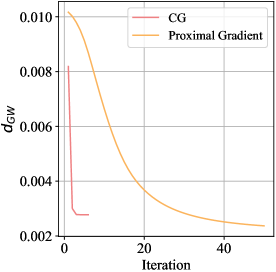
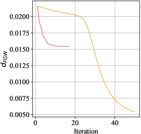
where and denotes the Hadamard product of matrix. and are two node attribute matrices. The proximal gradient algorithm [45] decomposes a complicated non-convex optimization problem into a series of convex sub-problems. The global convergence of this proximal gradient method is guaranteed in [46]. Algorithm 2 gives the pipeline of the proximal gradient algorithm. The conditional gradient algorithm [40] introduces a linear regularization term, where the solution provides a descent direction and a line-search whose optimal step can be found in closed form to update the FGW distance. Algorithm 3 gives the pipeline of the conditional gradient algorithm. Figure 6 shows the convergence of these two algorithms in computing the GW and FGW distances. It can be observed that the CG algorithm converges faster, but the proximal gradient converges to smaller values.
For the computation of the OT plan and the update the marginals and in the modality-level, Algorithm 4 gives the pipeline. It first solves via the Sinkhorn-scaling algorithm [8] and then updates the marginals.
Appendix B Derivation of (13)
For the sake of convenience, we denote as the optimal solution of , i.e.,
| (17) |
For the matrix , we denote its component as . Since , we have
| (18) |
which indicates that the result of is a constant independent of .
Assume that is fixed as a uniform distribution. In such a situation, we can find that
| (19) |
Then we prove the upper bound in equation 13 as follows
| (20) |
where
| (21) |
which is an nonnegative constant independent of (according to equation 18).
Based on the above derivation, we have
| (22) |
Appendix C More Experimental Results
In Figure 7, we explore the impact of the weight in FGW distance on all the datasets. The results show that UHOT-GM has good robustness for most values of . In particular, the best matching results are achieved on both ACM-DBLP and PPI datasets when . Similarly, the results in Figure 8 show that UHOT-GM is also robust to the weight in the range . In Figure 9, we visualize the corresponding node-level OT plans as a complement to the OT visualization results in the main paper.