Differential Equation Scaling Limits of
Shaped and Unshaped Neural Networks

Abstract

Recent analyses of neural networks with shaped activations (i.e. the activation function is scaled as the network size grows) have led to scaling limits described by differential equations. However, these results do not a priori tell us anything about “ordinary” unshaped networks, where the activation is unchanged as the network size grows. In this article, we find similar differential equation based asymptotic characterization for two types of unshaped networks.

• Firstly, we show that the following two architectures converge to the same infinite-depth-and-width limit at initialization: (i) a fully connected ResNet with a $d^{-1/2}$ factor on the residual branch, where $d$ is the network depth. (ii) a multilayer perceptron (MLP) with depth $d\ll$ width $n$ and shaped ReLU activation at rate $d^{-1/2}$.

• Secondly, for an unshaped MLP at initialization, we derive the first order asymptotic correction to the layerwise correlation. In particular, if $\rho_{\ell}$ is the correlation at layer $\ell$, then $q_{t}=\ell^{2}(1-\rho_{\ell})$ with $t=\frac{\ell}{n}$ converges to an SDE with a singularity at $t=0$.

These results together provide a connection between shaped and unshaped network architectures, and opens up the possibility of studying the effect of normalization methods and how it connects with shaping activation functions.

1 Introduction

Martens et al. (2021); Zhang et al. (2022) proposed transforming the activation function to be more linear as the neural network becomes larger in size, which significantly improved the speed of training deep networks without batch normalization. Based on the infinite-depth-and-width limit analysis of Li et al. (2022), the principle of these transformations can be roughly summarized as follows: choose an activation function $\varphi_{s}:\mathbb{R}\to\mathbb{R}$ as a perturbation of the identity map depending on the network width $n$ (or depth $d=n^{2p},p>0$)

$$\varphi_{s}(x)=x+\frac{1}{n^{p}}h(x)+O(n^{-2p})=x+\frac{1}{\sqrt{d}}h(x)+O(d^{-1})\,,$$ (1.1)

where for simplicity we will ignore the higher order terms for now. Li et al. (2022) also showed the limiting multilayer perceptron (MLP) can be described by a Neural Covariance stochastic differential equation (SDE). Furthermore, it appears the choice of $p=\frac{1}{2}$ is necessary to reach a non-degenerate nor trivial limit, at least when the depth-to-width ratio $\frac{d}{n}$ converges to a positive constant (see (Li et al., 2022, Proposition 3.4)).

Recently, Hayou & Yang (2023); Cirone et al. (2023) also studied the infinite-depth-and-width limit of a specific ResNet architecture (He et al., 2016). Most interestingly, the limit is described by an ordinary differential equation (ODE) very similar to the neural covariance SDE. Furthermore, Hayou & Yang (2023) showed the width and depth limits commute, i.e. no dependence on the depth-to-width ratio $\frac{d}{n}$. It is then natural to consider a more careful comparison and understanding of the two differential equations.

At the same time, Li et al. (2022) demonstrated the unshaped network also has an accurate approximation via a Markov chain. Jakub & Nica (2023) further studied the large width asymptotics of the Markov chain updates, where the transition kernel still depends on the width. Since the Markov chain quickly converges to a fixed point, it does not immediately appear to have a scaling limit. However, this motivates us to consider a modified scaling around the fixed point, so that we can recover a first order asymptotic correction term.

In this note, we provide two technical results that address both of the above questions. Both of the results are achieved by considering a modification of the scaling, which leads to the following results.

• Firstly, we demonstrate that shaping the activation has a close connection to ResNets, and the covariance ODE is in fact just the deterministic drift component of the covariance SDE. Furthermore, in the limit requires the scaled ratio of $\frac{d}{n^{2p}}$ to converge to a positive constant and $p\in(0,\frac{1}{2})$, the shaped MLP covariance also converges to the same ODE.

• Secondly, we analyze the correlation of an unshaped MLP, providing a derivation of the first order asymptotic correction. The correction term arises from rescaling the correlation $\rho_{\ell}$ in layer $\ell$ by $q_{\ell}=\ell^{2}(1-\rho_{\ell})$, and we show it is closely approximated by an SDE.

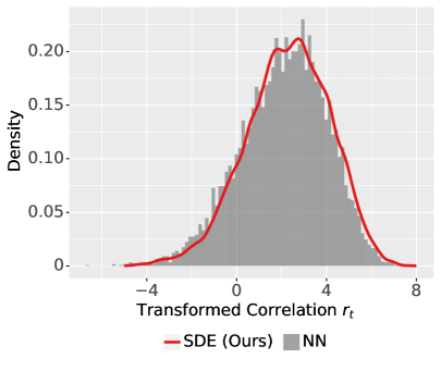
Figure 1: Empirical distribution of the transformed correlation $r_{t}=\log(\ell^{2}(1-\rho_{\ell}))$ for an unshaped ReLU MLP, SDE sample density computed via kernel density estimation. Simulated with $n=d=150,\rho_{0}=0.3,r_{0}=\log(1-\rho_{0})=\log(0.7)$, SDE step size $10^{-2}$, and $2^{13}$ samples.

The rest of this article is organized as follows. Firstly, we will provide a brief literature review in the rest of this section. Next, we will review the most relevant known results on this covariance SDEs and ODEs in Section 2. Then in Section 3, we will make the connection between shaping and ResNets precise. At the same time, we will also provide a derivation of the unshaped regime in Section 4, where we show that by modifying the scaling yet again, we can recover another SDE related to the correlation of a ReLU MLP.

1.1 Related Work

On a conceptual level, the main difficulty of neural networks is due to the lack of mathematical tractability. In a seminal work, Neal (1995) showed that two layer neural networks at initialization converges to a Gaussian process. Beyond the result itself, the conceptual breakthrough opened up the field to analyzing large size asymptotics of neural networks. In particular, this led to a large body of work on large or infinite width neural networks (Lee et al., 2018; Jacot et al., 2018; Du et al., 2019; Mei et al., 2018; Sirignano & Spiliopoulos, 2018; Yang, 2019; Bartlett et al., 2021). However, majority of these results relied on the network converging to a kernel limit, which are known to perform worse than neural networks (Ghorbani et al., 2020). The gap in performance is believed to be primarily due to a lack of feature learning (Yang & Hu, 2021; Abbe et al., 2022; Ba et al., 2022). While this motivated the study of several alternative scaling limits, in this work we are mostly interested in the infinite-depth-and-width limit.

First investigated by Hanin & Nica (2019b), it was shown that not only does this regime not converge to a Gaussian process at initialization, it also learns features Hanin & Nica (2019a). This limit has since been analyzed with transform based methods (Noci et al., 2021) and central limit theorem approaches (Li et al., 2021). As we will describe in more detail soon, the result of most interest is the covariance SDE limit of Li et al. (2022). The MLP results were also further extended to the transformer setting (Noci et al., 2023).

The $d^{-1/2}$ scaling for ResNets was first considered by Hayou et al. (2021), with the depth limit carefully studied afterwards (Hayou, 2022; Hayou & Yang, 2023; Hayou, 2023). Fischer et al. (2023) also arrived at the same scaling through a different theoretical approach. This scaling has found applications for hyperparameter tuning (Bordelon et al., 2023; Yang et al., 2023) when used in conjunction with the $\mu$P scaling (Yang & Hu, 2021).

Batch and layer normalization methods were introduced as a remedy for unstable training (Ioffe & Szegedy, 2015; Ba et al., 2016), albeit theoretical analyses of these highly discrete changes per layer has been challenging. A recent promising approach studies the isometry gap, and shows that batch normalization methods achieves a similar effect as shaping activation functions (Meterez et al., 2023). Theoretical connections between these approaches using a differential equation based description remains an open.

2 Existing Results on Shaped Network and ResNets

Let $\{x^{\alpha}\}_{\alpha=1}^{m}$ be a set of input data points in $\mathbb{R}^{{n_{\text{in}}}}$, and let $z^{\alpha}_{\ell}\in\mathbb{R}^{n}$ denote the $\ell$-th hidden layer with respect to the input $x^{\alpha}$. We consider the standard width-$n$ depth-$d$ MLP architecture with He-initialization (He et al., 2015) defined by the following recursion

$$z_{\text{out}}^{\alpha}=\sqrt{\frac{c}{n}}W_{\text{out}}\,\varphi(z_{d}^{\alpha})\,,\quad z_{\ell+1}^{\alpha}=\sqrt{\frac{c}{n}}W_{\ell}\,\varphi_{s}(z_{\ell}^{\alpha})\,,\quad z_{1}^{\alpha}=\frac{1}{\sqrt{{n_{\text{in}}}}}W_{\text{in}}\,x^{\alpha}\,,$$ (2.1)

where $\varphi_{s}:\mathbb{R}\to\mathbb{R}$ is applied entry-wise, $c^{-1}=\mathbb{E}\,\varphi_{s}(g)^{2}$ for $g\sim N(0,1)$, $z_{\ell}^{\alpha}\in\mathbb{R}^{n},z_{\text{out}}^{\alpha}\in\mathbb{R}^{{n_{\text{out}}}}$, and the matrices $W_{\text{out}}\in\mathbb{R}^{{n_{\text{out}}}\times n},W_{\ell}\in\mathbb{R}^{n\times n},W_{\text{in}}\in\mathbb{R}^{n\times{n_{\text{in}}}}$ are initialized with iid $N(0,1)$ entries.

The main results of Li et al. (2022) describes the limit as $d,n\to\infty$ with $\frac{d}{n}\to T>0$ and the activation function $\varphi$ is shaped to $\varphi_{s}$ depending on $n$ (Martens et al., 2021; Zhang et al., 2022). In particular, the covariance matrix $V_{\ell}:=\frac{c}{n}[\langle\varphi^{\alpha}_{\ell},\varphi^{\beta}_{\ell}\rangle]_{\alpha,\beta=1}^{m}$ with $\varphi^{\alpha}_{\ell}=\varphi_{s}(z^{\alpha}_{\ell})$ forms a Markov chain, and the main result describes the the limiting dynamics of $V_{\lfloor tn\rfloor}$ via a stochastic differential equation (SDE).

The activation functions are modified as follows. For a ReLU-like activation, we choose

$$\varphi_{s}(x)=s_{+}\max(x,0)+s_{-}\min(x,0)\,,\quad s_{\pm}=1+\frac{c_{\pm}}{n^{p}}\,,c_{\pm}\in\mathbb{R}\,,p\geq 0\,,$$ (2.2)

or for a smooth activation $\varphi\in C^{4}(\mathbb{R})$ such that $\varphi(0)=0,\varphi^{\prime}(0)=1$ and $\varphi^{(4)}(x)$ bounded by a polynomial, we choose

$$\varphi_{s}(x)=s\,\varphi\left(\frac{x}{s}\right)\,,\quad s=an^{p}\,,a\neq 0\,,p\geq 0\,.$$ (2.3)

We will first recall one of the main results of Li et al. (2022), which is stated informally below.

Theorem 2.1 (Theorem 3.2 and 3.9 of Li et al. (2022), Informal).

Let $p=\frac{1}{2}$. Then in the limit as $d,n\to\infty,\frac{d}{n}\to T>0$, and $\varphi_{s}$ defined as above, we have that the upper triangular entries of $V_{\lfloor tn\rfloor}$ (flattened to a vector) converges to the following SDE weakly

$$dV_{t}=b(V_{t})\,dt+\Sigma(V_{t})^{1/2}\,dB_{t}\,,\quad V_{0}=\frac{1}{{n_{\text{in}}}}[\langle x^{\alpha},x^{\beta}\rangle]_{\alpha,\beta=1}^{m}\,,$$ (2.4)

where $\Sigma(V)|_{\alpha\beta,\gamma\delta}=V^{\alpha\gamma}V^{\beta\delta}+V^{\alpha\delta}V^{\beta\gamma}$, and if $\varphi$ is a ReLU-like activation we have

$$b(V)|_{\alpha\beta}=\nu(\rho^{\alpha\beta})\sqrt{V^{\alpha\alpha}V^{\beta\beta}}\,,\quad\rho^{\alpha\beta}=\frac{V^{\alpha\beta}}{\sqrt{V^{\alpha\alpha}V^{\beta\beta}}}\,,\quad\nu(\rho)=\frac{(c_{+}-c_{-})^{2}}{2\pi}\left(\sqrt{1-\rho^{2}}-\rho\arccos\rho\right)\,,$$ (2.5)

or else if $\varphi$ is a smooth activation we have

$$b^{\alpha\beta}(V_{t})=\frac{\varphi^{\prime\prime}(0)^{2}}{4a^{2}}\left(V^{\alpha\alpha}_{t}V^{\beta\beta}_{t}+V^{\alpha\beta}_{t}(2V^{\alpha\beta}_{t}-3)\right)+\frac{\varphi^{\prime\prime\prime}(0)}{2a^{2}}V^{\alpha\beta}_{t}(V^{\alpha\alpha}_{t}+V^{\beta\beta}_{t}-2)\,.$$ (2.6)

At the same time, Hayou & Yang (2023); Cirone et al. (2023) found an ordinary differential equation (ODE) limit describing the covariance matrix for infinite-depth-and-width ResNets. The authors considered a ResNet architecture with a $\frac{1}{\sqrt{d}}$ factor on their residual branch, more precisely their recursion is defined as follows (in our notation and convention)

$$z^{\alpha}_{\ell+1}=z^{\alpha}_{\ell}+\frac{1}{\sqrt{dn}}W_{\ell}\,\varphi(z^{\alpha}_{\ell})\,,\quad\text{ where }\varphi(x)=\max(x,0)\,.$$ (2.7)

One of their main results can be stated informally as follows.

Theorem 2.2 (Theorem 2 of Hayou & Yang (2023), Informal).

Let $d,n\to\infty$ (in any order), and the covariance process $V^{\alpha\beta}_{\lfloor td\rfloor}$ converges to the following ODE

$$\frac{d}{d_{t}}V^{\alpha\beta}_{t}=\frac{1}{2}\frac{f(\rho^{\alpha\beta}_{t})}{\rho^{\alpha\beta}_{t}}V_{t}^{\alpha\beta}\,,$$ (2.8)

where $f(\rho)=\frac{1}{\pi}(\rho\arcsin\rho+\sqrt{1-\rho^{2}})+\frac{1}{2}\rho$.

Here, we observe this ODE (2.8) is exactly the drift component of the covariance SDE (2.4), i.e.

$$\frac{1}{2}\frac{f(\rho^{\alpha\beta}_{t})}{\rho^{\alpha\beta}_{t}}V_{t}^{\alpha\beta}=\nu(\rho^{\alpha\beta}_{t})\sqrt{V^{\alpha\alpha}_{t}V^{\beta\beta}_{t}}\,,\quad\text{ if }(c_{+}-c_{-})^{2}=1\,,\frac{d}{n}=1\,.$$ (2.9)

To see this, we just need to use the identity $\arcsin\rho=\frac{\pi}{2}-\arccos\rho$ to get that $\frac{1}{2}f(\rho)=\nu(\rho)$, and that $\frac{V^{\alpha\beta}_{t}}{\rho^{\alpha\beta}_{t}}=\sqrt{V^{\alpha\alpha}_{t}V^{\beta\beta}_{t}}$ is exactly the definition of $\rho^{\alpha\beta}_{t}$. We also note the correlation ODE $\frac{d}{dt}\rho^{\alpha\beta}_{t}=\nu(\rho^{\alpha\beta}_{t})$ was first derived in (Zhang et al., 2022, Proposition 3), where they considered the sequential width then depth limit with a fixed initial and terminal condition.

In the next section, we will describe another way to recover this ODE from an alternative scaling limit of the shaped MLP.

3 An Alternative Shaped Limit for $p\in(0,\frac{1}{2})$

We start by providing some intuitions on this result. The shaped MLP can be seen as a layerwise perturbation of the linear network

$$z_{\ell+1}=\sqrt{\frac{c}{n}}W_{\ell}\,\varphi_{s}(z_{\ell})\approx\sqrt{\frac{c}{n}}W_{\ell}\,z_{\ell}+\frac{1}{\sqrt{d}}\sqrt{\frac{c}{n}}W_{\ell}\,h(z_{\ell})\,,$$ (3.1)

where $c^{-1}=\mathbb{E}\,\varphi_{s}(g)^{2}$ for $g\sim N(0,1)$ corresponds to the He-initialization (He et al., 2015), and $W_{\ell}\in\mathbb{R}^{n\times n}$ has iid $N(0,1)$ entries.

On an intuitive level (which we will make precise in Remark 3.3), if we take the infinite-width limit first, then this removes the effect of the random weights. In other words, if we replace the weights $\frac{1}{\sqrt{n}}W_{\ell}$ with the identity matrix $I_{n}$ in each hidden layer, we get the same limit at initialization. Therefore, we can heuristically write

$$z_{\ell+1}\approx z_{\ell}+\frac{1}{\sqrt{d}}h(z_{\ell})\,,$$ (3.2)

where we also used the fact $c\to 1$ in the limit.

Observe this is resembling a ResNet, where the first $z_{\ell}$ is the skip connection. In fact, we can again heuristically add back in the weights on the residual branch to get

$$z_{\ell+1}\approx z_{\ell}+\frac{1}{\sqrt{d}}W_{\ell}h(z_{\ell})\,,$$ (3.3)

which exactly recovers the ResNet formulation of Hayou et al. (2021); Hayou & Yang (2023), where the authors studied the case when $h(x)=\max(x,0)$ is the ReLU activation.

Remark 3.1.

On a heuristic level, this implies that whenever the width limit is taken first (or equivalently $d=n^{2p}$ for $p\in(0,1/2)$), the shaped network with shaping parameter $d^{-1/2}$ has the same limiting distribution at initialization as a ResNet with a $d^{-1/2}$ weighting on the residual branch.

However, we note that despite having identical ODE for the covariance at initialization, this does not imply the training dynamics will be the same — it will likely be different. Furthermore, since Hayou & Yang (2023) showed the width and depth limits commute for ResNets, this provides the additional insight that noncommunitativity of limits in shaped MLPs arises from the product of random matrices.

3.1 Precise Results

The core object that forms a Markov chain is the post-activation covariance matrix $\frac{c}{n}[\langle\varphi^{\alpha}_{\ell},\varphi^{\beta}_{\ell}\rangle]_{\alpha,\beta=1}^{m}$. To see this, we will use the property of Gaussian matrix multiplication, where we let $W\in\mathbb{R}^{n\times n}$ with iid entries $W_{ij}\sim N(0,1)$, and $\{u^{\alpha}\}_{\alpha=1}^{m}\in\mathbb{R}^{n}$ be a collection of constant vectors, which gives us

$$[Wu^{\alpha}]_{\alpha=1}^{m}\overset{d}{=}N(0,[\langle u^{\alpha},u^{\beta}\rangle]_{\alpha=1}^{m}\otimes I_{n})\,,$$ (3.4)

where we use the notation $[v^{\alpha}]_{\alpha=1}^{m}$ to stack the vectors vertically. This forms a Markov chain because we can condition on $\mathcal{F}_{\ell}=\sigma([z^{\alpha}_{\ell}]_{\alpha=1}^{m})$ to get

$$[z^{\alpha}_{\ell+1}]_{\alpha=1}^{m}|\mathcal{F}_{\ell}=[z^{\alpha}_{\ell+1}]_{\alpha=1}^{m}|\sigma(V_{\ell})\sim N(0,V_{\ell}\otimes I_{n})\,.$$ (3.5)

and we can see that $V_{\ell+1}|\mathcal{F}_{\ell}=V_{\ell+1}|\sigma(V_{\ell})$, which is exactly the definition of a Markov chain.

We will start with a quick Lemma.

Lemma 3.2 (Covariance Markov Chain for the Shaped MLP).

Let $z^{\alpha}_{\ell}$ be the MLP in defined in Equation 2.1 with shaped ReLU activations defined in Equation 2.2. For $p\in(0,\frac{1}{2})$ and $d=n^{2p}$, the Markov chain satisfies

$$V_{\ell+1}=V_{\ell}+\frac{b_{s}(V_{\ell})}{d}+\frac{\Sigma_{s}(V_{\ell})^{1/2}\,\xi_{\ell}}{\sqrt{n}}+O(d^{-3/2}+n^{-3/2})\,,$$ (3.6)

where $\{\xi_{\ell}\}_{\ell\geq 0}$ are iid zero mean and identity covariance random vectors, and in the limit as $n,d\to\infty$ we have that $b_{s}\to b$ and $\Sigma_{s}\to\Sigma$ defined in Theorem 2.1.

Proof.

We will first adapt (Li et al., 2022, Lemma C.1). For $\rho\in[-1,1]$, let

$$\begin{bmatrix}g\\ \hat{g}\end{bmatrix}\sim N\left(0\,,\begin{bmatrix}1&\rho\\ \rho&1\end{bmatrix}\,\right)\,,$$ (3.7)

we have that $K_{1}(\rho)=\mathbb{E}\,\varphi_{s}(g)\varphi_{s}(\hat{g})$ satisfies

$$cK_{1}(\rho)=\rho+\frac{\nu(\rho)}{n^{2p}}+O(n^{-3p})\,,$$ (3.8)

where $\nu(\rho)$ is defined in Theorem 2.1.

The rest follows directly from the calculations in the proof of (Li et al., 2022, Theorem 3.2), where we just need to replace $cK_{1}(\rho^{\alpha\beta}_{\ell})$ with the above.

∎

Remark 3.3.

We note that the drift term arising from the activation depends only on the depth $d$ and the random term only depends on the width $n$. If we decouple the dependence on $d$ and $n$, and take the infinite-width limit first, we arrive at

$$V_{\ell+1}=V_{\ell}+\frac{b_{s}(V_{\ell})}{d}+O(n^{-3/2})\,,$$ (3.9)

which is equivalent to removing the randomness of the weights.

We note this Markov chain behaves like a sum of two Euler updates with step sizes $\frac{1}{n^{2p}}$ and $\frac{1}{n}$, where the $\frac{1}{n}$ corresponds to the random term with coefficient $\frac{1}{\sqrt{n}}$. However since $p\in(0,\frac{1}{2})$, the first term with step size $\frac{1}{n^{2p}}$ will dominate, which is the term that corresponds to shaping the activation function. Therefore, using the Markov chain convergence to SDE result in (Li et al., 2022, Proposition A.6), we will recover the ODE result.

Proposition 3.4 (Covariance ODE for the Shaped ReLU MLP).

Let $p\in(0,\frac{1}{2})$. Then in the limit as $d,n\to\infty,\frac{d}{n^{2p}}\to 1$, and $\varphi_{s}$ is the shaped ReLU defined in Equation 2.2, we have that the upper triangular entries of $V_{\lfloor tn\rfloor}$ (flattened to a vector) converges to the following ODE weakly

$$dV_{t}=b(V_{t})\,dt\,,\quad V_{0}=\frac{1}{{n_{\text{in}}}}[\langle x^{\alpha},x^{\beta}\rangle]_{\alpha,\beta=1}^{m}\,,$$ (3.10)

where $b$ is defined in Theorem 2.1.

Proof.

Follows from an application of (Li et al., 2022, Proposition A.6) to the Markov chain in Equation 3.6.

∎

At this point it’s worth pointing out the regime of $p\in(0,\frac{1}{2})$ was studied in Li et al. (2022), but the scaling limit was taken to be $\frac{d}{n}\to T$ instead of $\frac{d}{n^{2p}}$. This led to a “degenerate” regime where $\rho_{t}=1$ for all $t>0$. The above ODE result implies that the degenerate limit can be characterized in a more refined way if the scaling is chosen carefully.

In the next and final section, we show that actually even when the network is unshaped (i.e. $p=0$), there exists a scaling such that we can characterize the limiting Markov chain up to the first order asymptotic correction.

4 An SDE for the Unshaped ReLU MLP

In this section, we let $\varphi_{s}(x)=\varphi(x)=\max(x,0)$, and we are interested in studying the correlation

$$\rho^{\alpha\beta}_{\ell}=\frac{V^{\alpha\beta}_{\ell}}{\sqrt{V^{\alpha\alpha}_{\ell}V^{\beta\beta}_{\ell}}}=\frac{\langle\varphi^{\alpha}_{\ell},\varphi^{\beta}_{\ell}\rangle}{|\varphi^{\alpha}_{\ell}|\,|\varphi^{\beta}_{\ell}|}\,.$$ (4.1)

From this point onwards, we will only consider the marginal over two inputs, so we will drop the superscript $\alpha\beta$. Similar to the previous section, we will also start by providing an intuitive sketch.

Many existing work has derived the rough asymptotic order of the unshaped correlation to be $\rho_{\ell}=1-O(\ell^{-2})$, where $\ell$ is the layer (see for example Appendix E of Li et al. (2022) and Jakub & Nica (2023)). Firstly, this implies that a Taylor expansion of all functions of $\rho$ in the Markov chain update around $\rho=1$ will be very accurate. At the same time, it is natural to magnify the object inside the big $O$ by reverting the scaling, or more precisely consider the object

$$q_{\ell}=\ell^{2}(1-\rho_{\ell})\,,$$ (4.2)

which will hopefully remain at size $\Theta(1)$.

For simplicity, we can consider the infinite-width update of the unshaped correlation (which corresponds to the zeroth-order Taylor expansion in $\frac{1}{n}$)

$$\rho_{\ell+1}=\rho_{\ell}+c_{1}(1-\rho_{\ell})^{3/2}+O((1-\rho_{\ell})^{5/2})\,,$$ (4.3)

where for the sake of illustration we will take $c_{1}=1$ and drop the big $O$ term for now. Substituting in $q_{\ell}$, we can recover the update

$$q_{\ell+1}=q_{\ell}+\frac{2q_{\ell}}{\ell}-\frac{q_{\ell}^{3/2}}{\ell}\,.$$ (4.4)

While this doesn’t quite look like an Euler update just yet, we can substitute in $t=\frac{\ell}{n}$ for the time scale, which will lead us to have

$$q_{\ell+1}=q_{\ell}+\frac{1}{tn}\left(2q_{\ell}-q_{\ell}^{3/2}\right)\,,$$ (4.5)

hence (heuristically) giving us the singular ODE

$$dq_{t}=\frac{2q_{t}-q_{t}^{3/2}}{t}\,.$$ (4.6)

To recover the SDE, we will simply include the additional terms of the Markov chain instead taking the infinite-width limit first.

4.1 Full Derivation

In the rest of this section, we will provide a derivation of an SDE arising from an appropriate scaling of $\rho_{\ell}$.

Theorem 4.1 (Rescaled Correlation).

Let $q_{\ell}=\ell^{2}(1-\rho_{\ell})$. Then for all $t_{0}>0$, the process $\{q_{\lfloor tn\rfloor}\}_{t\geq t_{0}}$ converges to a solution of the following SDE weakly in the Skorohod topology (see (Li et al., 2022, Appendix A))

$$dq_{t}=2q_{t}\left(\frac{1-\frac{\sqrt{2}}{3\pi}q_{t}^{1/2}}{t}-1\right)\,dt+2\sqrt{2}q_{t}\,dB_{t}\,.$$ (4.7)

The above statement holds only when $t_{0}>0$, and there is a interesting technicality that must be resolved to interpret what happens as $t\to 0^{+}$. In particular, the Markov chain is not time homogeneous, and the limiting SDE has a singularity at $t=0$. The contribution of the singularity needs to be controlled in order to establish convergence for all $t\geq 0$. Furthermore, due to the singularity issue, it is also unclear what the initial condition of $q_{t}$ should be.

In our simulations for Figure 1, we addressed the time singularity by shifting the time evaluation of $\frac{1}{t}$ to the next step of $\frac{1}{t+\Delta_{t}}$, where $\Delta_{t}>0$ is the time step size. More precisely, we first consider the log version of $r_{t}=\log q_{t}$

$$dr_{t}=-2\left(1-\frac{1-\frac{\sqrt{2}}{3\pi}\exp(\frac{r_{t}}{2})}{t}\right)\,dt+2\sqrt{2}dB_{t}\,.$$ (4.8)

Then we choose the following discretization

$$r_{t+\Delta_{t}}=r_{t}-2\left(1-\frac{1-\frac{\sqrt{2}}{3\pi}\exp(\frac{r_{t}}{2})}{t+\Delta_{t}}\right)\,\Delta_{t}+2\sqrt{2}\,\xi_{t}\sqrt{\Delta_{t}}\,,$$ (4.9)

where $\xi_{t}\sim N(0,1)$. For initial conditions, we also noticed that since the initial correlation must be contained in the interval $[-1,1]$, the end result was not very sensitive to the choice of $r_{0}$.

of Theorem 4.1.

Firstly, we will introduce the definitions

$$K_{p,r}(\rho) =\mathbb{E}\,\varphi_{s}(g)^{p}\varphi_{s}(\hat{g})^{r}\,,$$ (4.10)

where $g,w\sim N(0,1)$ and we define $\hat{g}=\rho g+qw$ with $q=\sqrt{1-\rho^{2}}$. We will also use the short hand notation to write $K_{p}:=K_{p,p}$. Here we will recall several formulae calculated in Cho & Saul (2009) and (Li et al., 2022, Lemma B.4)

$$K_{0}(\rho) =\mathbb{E}\,\mathds{1}_{\{g>0\}}\mathds{1}_{\{\rho g+qw>0\}}=\frac{\arccos(-\rho)}{2\pi}\,,$$ (4.11)

$$K_{1}(\rho) =\mathbb{E}\,\varphi(g)\varphi(\rho g+qw)=\frac{q+\rho\arccos(-\rho)}{2\pi}\,,$$

$$K_{2}(\rho) =\mathbb{E}\,\varphi(g)^{2}\varphi(\rho g+qw)^{2}=\frac{3\rho q+\arccos(-\rho)(1+2\rho^{2})}{2\pi}\,,$$

$$K_{3,1}(\rho) =\mathbb{E}\,\varphi(g)^{3}\varphi(\rho g+qw)=\frac{q(2+\rho^{2})+3\arccos(-\rho)\rho}{2\pi}\,.\,.$$

Furthermore, we will define

$$M_{2}\coloneqq\mathbb{E}\,[c\varphi(g)^{2}-1]^{2}=5\,.$$ (4.12)

Using the steps of (Li et al., 2022, Proposition B.8), we can establish an approximate Markov chain

$$\rho_{\ell+1}=cK_{1}(\rho_{\ell})+\frac{\widehat{\mu}_{r}(\rho_{\ell})}{n}+\frac{\sigma_{r}(\rho_{\ell})\xi_{\ell}}{\sqrt{n}}+O(n^{-3/2})\,,$$ (4.13)

where $\xi_{\ell}$ are iid with zero mean and unit variance, and

$$\mu_{r}(\rho_{\ell}) =\mathbb{E}[\,\widehat{\mu}_{r}(\rho_{\ell})|\rho_{\ell}]=\frac{c}{4}\left[K_{1}(c^{2}K_{2}+3M_{2}+3)-4cK_{3,1}\right]\,,$$ (4.14)

$$\sigma_{r}^{2}(\rho_{\ell}) =\frac{c^{2}}{2}\left[K_{1}^{2}(c^{2}K_{2}+M_{2}+1)-4cK_{1}K_{3,1}+2K_{2}\right]\,,$$

and we write $K_{\cdot}=K_{\cdot}(\rho_{\ell})$.

Here we use the big $O(f(n,\ell))$ to denote a random variable $X$ such that for all $p\geq 1$

$$\frac{\mathbb{E}|X|^{p}}{f(n,\ell)^{p}}\leq C_{p}<\infty\,,$$ (4.15)

for some constants $C_{p}>0$ independent of $n$ and $\ell$.

In view of the SDE convergence theorem (Li et al., 2022, Proposition A.6), if we eventually reach an SDE, we will only need to keep track of the expected drift $\mu_{r}$ instead of the random drift. We can then Taylor expand the coefficients in terms of $\rho_{\ell}$ about $\rho_{\ell}=1$ (from the negative direction) using SymPy (Meurer et al., 2017), which translates to the following update rule

$$\rho_{\ell+1} =\rho_{\ell}+\frac{2\sqrt{2}}{3\pi}(1-\rho_{\ell})^{3/2}+\frac{\sqrt{2}}{30\pi}(1-\rho_{\ell})^{5/2}$$ (4.16)

$$\quad+\frac{1}{n}\left(-2(1-\rho_{\ell})+\frac{4\sqrt{2}}{\pi}(1-\rho_{\ell})^{3/2}+3(1-\rho_{\ell})^{2}-\frac{73\sqrt{2}}{15\pi}(1-\rho_{\ell})^{5/2}\right)$$

$$\quad+\frac{\xi_{\ell}}{\sqrt{n}}\left(2\sqrt{2}(1-\rho_{\ell})-\frac{56}{15\pi}(1-\rho_{\ell})^{3/2}\right)+O((1-\rho_{\ell})^{4}+n^{-3/2})\,.$$

We note up to this point, a similar approach was taken in Jakub & Nica (2023). However, we will diverge here by consider the following scaling

$$q_{\ell}=\ell^{2}(1-\rho_{\ell})\,.$$ (4.17)

The choice of $\ell^{2}$ scale is motivated by the infinite-width limit, where $(1-\rho_{\ell})$ shown to be of order $O(\ell^{-2})$ in (Li et al., 2022, Appendix E). This implies the following update

$$\frac{\ell^{2}}{(\ell+1)^{2}}q_{\ell+1} =q_{\ell}-\ell^{2}\frac{2\sqrt{2}}{3\pi}(1-\rho_{\ell})^{3/2}-\ell^{2}\frac{\sqrt{2}}{30\pi}(1-\rho_{\ell})^{5/2}$$ (4.18)

$$\quad-\frac{\ell^{2}}{n}\left(-2(1-\rho_{\ell})+\frac{4\sqrt{2}}{\pi}(1-\rho_{\ell})^{3/2}+3(1-\rho_{\ell})^{2}-\frac{73\sqrt{2}}{15\pi}(1-\rho_{\ell})^{5/2}\right)$$

$$\quad+\frac{\xi_{\ell}\ell^{2}}{\sqrt{n}}\left(2\sqrt{2}(1-\rho_{\ell})-\frac{56}{15\pi}(1-\rho_{\ell})^{3/2}\right)+O(\ell^{-8}q_{\ell}^{4}+\ell^{-2}n^{-3/2})\,.$$

Next, we will drop all higher order terms in $\ell$, then using the fact that $\frac{\ell^{2}}{(\ell+1)^{2}}=1-\frac{2}{\ell}+O(\ell^{-2})$, we can write

$$q_{\ell+1}=q_{\ell}(1+2\ell^{-1})-\frac{2\sqrt{2}}{3\pi}\frac{q_{\ell}^{3/2}}{\ell}-\frac{2q_{\ell}}{n}+\frac{\xi_{\ell}}{\sqrt{n}}2\sqrt{2}q_{\ell}+O(\ell^{-2}+n^{-1/2}\ell^{-1})\,,$$ (4.19)

where we dropped $\ell^{-2}n^{-3/2}$ in the big $O$ since it gets dominated by $\ell^{-2}$.

Choosing the time scaling $t=\frac{\ell}{n}$ then gives us

$$q_{\ell+1}=q_{\ell}+\frac{2}{n}q_{\ell}\left(\frac{1-\frac{\sqrt{2}}{3\pi}q_{\ell}^{1/2}}{t}-1\right)+2\sqrt{\frac{2}{n}}q_{\ell}\,\xi_{\ell}+O(t^{-2}n^{-2}+t^{-1}n^{-3/2})\,.$$ (4.20)

Finally, we will use the Markov chain convergence result to an SDE result from (Li et al., 2022, Proposition A.6), which leads to the desired SDE for $t\geq t_{0}>0$

$$dq_{t}=2q_{t}\left(\frac{1-\frac{\sqrt{2}}{3\pi}q_{t}^{1/2}}{t}-1\right)\,dt+2\sqrt{2}q_{t}\,dB_{t}\,.$$ (4.21)

∎

References

- Abbe et al. (2022) Emmanuel Abbe, Enric Boix Adsera, and Theodor Misiakiewicz. The merged-staircase property: a necessary and nearly sufficient condition for sgd learning of sparse functions on two-layer neural networks. In Conference on Learning Theory, pp. 4782–4887. PMLR, 2022.
- Ba et al. (2022) Jimmy Ba, Murat A Erdogdu, Taiji Suzuki, Zhichao Wang, Denny Wu, and Greg Yang. High-dimensional asymptotics of feature learning: How one gradient step improves the representation. arXiv preprint arXiv:2205.01445, 2022.
- Ba et al. (2016) Jimmy Lei Ba, Jamie Ryan Kiros, and Geoffrey E Hinton. Layer normalization. arXiv preprint arXiv:1607.06450, 2016.
- Bartlett et al. (2021) Peter L Bartlett, Andrea Montanari, and Alexander Rakhlin. Deep learning: a statistical viewpoint. Acta numerica, 30:87–201, 2021.
- Bordelon et al. (2023) Blake Bordelon, Lorenzo Noci, Mufan Bill Li, Boris Hanin, and Cengiz Pehlevan. Depthwise hyperparameter transfer in residual networks: Dynamics and scaling limit, 2023.
- Cho & Saul (2009) Youngmin Cho and Lawrence K Saul. Kernel methods for deep learning. In Advances in Neural Information Processing Systems (NeurIPS), pp. 342–350, 2009.
- Cirone et al. (2023) Nicola Muca Cirone, Maud Lemercier, and Cristopher Salvi. Neural signature kernels as infinite-width-depth-limits of controlled resnets. arXiv preprint arXiv:2303.17671, 2023.
- Du et al. (2019) Simon Du, Jason Lee, Haochuan Li, Liwei Wang, and Xiyu Zhai. Gradient descent finds global minima of deep neural networks. In Int. Conf. Machine Learning (ICML), pp. 1675–1685. PMLR, 2019.
- Fischer et al. (2023) Kirsten Fischer, David Dahmen, and Moritz Helias. Optimal signal propagation in resnets through residual scaling. arXiv preprint arXiv:2305.07715, 2023.
- Ghorbani et al. (2020) Behrooz Ghorbani, Song Mei, Theodor Misiakiewicz, and Andrea Montanari. When do neural networks outperform kernel methods? Advances in Neural Information Processing Systems, 33:14820–14830, 2020.
- Hanin & Nica (2019a) Boris Hanin and Mihai Nica. Finite depth and width corrections to the neural tangent kernel. In Int. Conf. Learning Representations (ICLR), 2019a.
- Hanin & Nica (2019b) Boris Hanin and Mihai Nica. Products of many large random matrices and gradients in deep neural networks. Communications in Mathematical Physics, pp. 1–36, 2019b.
- Hayou (2022) Soufiane Hayou. On the infinite-depth limit of finite-width neural networks. Transactions on Machine Learning Research, 2022.
- Hayou (2023) Soufiane Hayou. Commutative width and depth scaling in deep neural networks, 2023.
- Hayou & Yang (2023) Soufiane Hayou and Greg Yang. Width and depth limits commute in residual networks. arXiv preprint arXiv:2302.00453, 2023.
- Hayou et al. (2021) Soufiane Hayou, Eugenio Clerico, Bobby He, George Deligiannidis, Arnaud Doucet, and Judith Rousseau. Stable ResNet. In Int. Conf. Artificial Intelligence and Statistics (AISTATS), pp. 1324–1332. PMLR, 2021.
- He et al. (2015) Kaiming He, Xiangyu Zhang, Shaoqing Ren, and Jian Sun. Delving deep into rectifiers: Surpassing human-level performance on imagenet classification. In Proc. IEEE Int. Conf. Computer Vision, pp. 1026–1034, 2015.
- He et al. (2016) Kaiming He, Xiangyu Zhang, Shaoqing Ren, and Jian Sun. Deep residual learning for image recognition. In Proceedings of the IEEE conference on computer vision and pattern recognition, pp. 770–778, 2016.
- Ioffe & Szegedy (2015) Sergey Ioffe and Christian Szegedy. Batch normalization: Accelerating deep network training by reducing internal covariate shift. In International conference on machine learning, pp. 448–456. pmlr, 2015.
- Jacot et al. (2018) Arthur Jacot, Franck Gabriel, and Clément Hongler. Neural tangent kernel: Convergence and generalization in neural networks. In Advances in Information Processing Systems (NeurIPS), 2018.
- Jakub & Nica (2023) Cameron Jakub and Mihai Nica. Depth degeneracy in neural networks: Vanishing angles in fully connected relu networks on initialization. arXiv preprint arXiv:2302.09712, 2023.
- Lee et al. (2018) Jaehoon Lee, Yasaman Bahri, Roman Novak, Samuel S Schoenholz, Jeffrey Pennington, and Jascha Sohl-Dickstein. Deep neural networks as gaussian processes. In Int. Conf. Learning Representations (ICLR), 2018.
- Li et al. (2021) Mufan Li, Mihai Nica, and Dan Roy. The future is log-gaussian: Resnets and their infinite-depth-and-width limit at initialization. Advances in Neural Information Processing Systems, 34, 2021.
- Li et al. (2022) Mufan Bill Li, Mihai Nica, and Daniel M Roy. The neural covariance sde: Shaped infinite depth-and-width networks at initialization. arXiv preprint arXiv:2206.02768, 2022.
- Martens et al. (2021) James Martens, Andy Ballard, Guillaume Desjardins, Grzegorz Swirszcz, Valentin Dalibard, Jascha Sohl-Dickstein, and Samuel S Schoenholz. Rapid training of deep neural networks without skip connections or normalization layers using deep kernel shaping. arXiv preprint arXiv:2110.01765, 2021.
- Mei et al. (2018) Song Mei, Andrea Montanari, and Phan-Minh Nguyen. A mean field view of the landscape of two-layer neural networks. Proceedings of the National Academy of Sciences, 115(33):E7665–E7671, 2018.
- Meterez et al. (2023) Alexandru Meterez, Amir Joudaki, Francesco Orabona, Alexander Immer, Gunnar Rätsch, and Hadi Daneshmand. Towards training without depth limits: Batch normalization without gradient explosion, 2023.
- Meurer et al. (2017) Aaron Meurer, Christopher P. Smith, Mateusz Paprocki, Ondřej Čertík, Sergey B. Kirpichev, Matthew Rocklin, AMiT Kumar, Sergiu Ivanov, Jason K. Moore, Sartaj Singh, Thilina Rathnayake, Sean Vig, Brian E. Granger, Richard P. Muller, Francesco Bonazzi, Harsh Gupta, Shivam Vats, Fredrik Johansson, Fabian Pedregosa, Matthew J. Curry, Andy R. Terrel, Štěpán Roučka, Ashutosh Saboo, Isuru Fernando, Sumith Kulal, Robert Cimrman, and Anthony Scopatz. Sympy: symbolic computing in python. PeerJ Computer Science, 3:e103, January 2017. ISSN 2376-5992. doi: 10.7717/peerj-cs.103. URL https://doi.org/10.7717/peerj-cs.103.
- Neal (1995) Radford M Neal. Bayesian learning for neural networks, volume 118. Springer Science & Business Media, 1995.
- Noci et al. (2021) Lorenzo Noci, Gregor Bachmann, Kevin Roth, Sebastian Nowozin, and Thomas Hofmann. Precise characterization of the prior predictive distribution of deep relu networks. Advances in Neural Information Processing Systems, 34, 2021.
- Noci et al. (2023) Lorenzo Noci, Chuning Li, Mufan Bill Li, Bobby He, Thomas Hofmann, Chris Maddison, and Daniel M Roy. The shaped transformer: Attention models in the infinite depth-and-width limit. arXiv preprint arXiv:2306.17759, 2023.
- Sirignano & Spiliopoulos (2018) Justin Sirignano and Konstantinos Spiliopoulos. Mean field analysis of neural networks: A law of large numbers, 2018.
- Yang (2019) Greg Yang. Tensor programs i: Wide feedforward or recurrent neural networks of any architecture are gaussian processes, 2019.
- Yang & Hu (2021) Greg Yang and Edward J. Hu. Feature learning in infinite-width neural networks. In Int. Conf. Machine Learning (ICML), 2021.
- Yang et al. (2023) Greg Yang, Dingli Yu, Chen Zhu, and Soufiane Hayou. Tensor programs vi: Feature learning in infinite-depth neural networks, 2023.
- Zhang et al. (2022) Guodong Zhang, Aleksandar Botev, and James Martens. Deep learning without shortcuts: Shaping the kernel with tailored rectifiers. arXiv preprint arXiv:2203.08120, 2022.