Out-of-equilibrium simulations to fight topological freezing

Abstract

Calculations of topological observables in lattice gauge theories with traditional Monte Carlo algorithms have long been known to be a difficult task, owing to the effects of long autocorrelations times. Several mitigation strategies have been put forward, including the use of open boundary conditions and methods such as parallel tempering. In this contribution we examine a new approach based on out-of-equilibrium Monte Carlo simulations. Starting from thermalized configurations with open boundary conditions on a line defect, periodic boundary conditions are gradually switched on. A sampling of topological observables is then shown to be possible with a specific reweighting-like technique inspired by Jarzynski’s equality. We discuss the efficiency of this approach using results obtained for the 2-dimensional $\text{CP}^{N-1}$ models. Furthermore, we outline the implementation of our proposal in the context of Stochastic Normalizing Flows, as they share the same theoretical framework of the non-equilibrium transformations we perform, and can be thought of as their generalization.

1 Introduction

At very fine lattice spacing, the vacuum of Lattice regularized QCD with periodic boundary conditions is well known to be characterized by the emergence of topological sectors. These are labeled by different values of the topological charge $Q$, and are separated by energy barriers whose height tends to infinity as the continuum limit is approached. As the lattice spacing is reduced, standard Markov Chain Monte Carlo (MCMC) algorithms based on local updating algorithms becomes less and less efficient in overcoming these barriers, and, eventually the Markov chain remains trapped in a fixed topological sector. This phenomenon, known as “topological freezing”, causes topological quantities to suffer from very long autocorrelation times, that increase exponentially as the continuum limit is approached, see Refs. [1, 2, 3, 4, 5, 6, 7, 8, 9, 10, 11, 12, 13, 14].

A strategy to mitigate this issue is provided by Open Boundary Conditions (OBC) in the temporal direction, see Refs. [15, 16], that effectively remove the barriers between topological sectors: in MCMC simulations with such boundary conditions, topological observables feature much smaller autocorrelation times. Yet, OBC induce sizeable finite-size effects, and relevant observables can be computed only on portions of the volume far enough from the boundaries. Moreover, a notion of global topological charge is lost. Another promising alternative proposed to mitigate topological freezing is known as Parallel Tempering on Boundary Conditions (PTBC), see Ref. [17]: in this state-of-the-art approach, replicas with different boundary conditions, interpolating from open to periodic, are simulated simultaneously and configurations of neighbouring replicas are swapped using a Metropolis step. This allows for an efficient sampling of topological observables on the replica with periodic boundary conditions (PBC), by exploiting the relatively short autocorrelation time of the replica with OBC and bypassing complications introduced by OBC.

In this contribution, we propose a new MCMC method based on out-of-equilibrium evolutions inspired by Jarzynski’s equality, see Ref. [18], a well known result in non-equilibrium statistical mechanics. This approach has been widely used in lattice field theory as well, namely in the computation of interface free energies, see Ref. [19], of the equation of state, see Ref. [20], of the renormalized coupling of gauge theories, see Ref. [21], and of the entanglement entropy of lattice field theories, see Ref. [22]. Moreover, it has also been combined with Normalizing Flows (see Ref. [23]), a deep-learning architecture that has been recently applied to lattice field theories: see Ref. [24] for an introduction. In this new framework, called Stochastic Normalizing Flows (SNFs), see Refs. [25, 26], MCMC updates that compose out-of-equilibrium evolutions are combined with discrete coupling layers, i.e. the building blocks that compose Normalizing Flows, resulting in an improvement of the purely stochastic approach.

In the context of topological freezing mitigation, out-of-equilibrium evolutions can leverage the advantages of OBC–small autocorrelation times–while avoiding its pitfalls–the complication introduced by the boundaries–by a direct sampling of the PBC theory via an appropriate reweighting-like technique. In the following, we test this method on the $\mathrm{CP}^{N-1}$ models in two dimensions, and perform a direct comparison with results obtained in the same setting using the PTBC.

2 Out-of-equilibrium evolutions

Consider a family of actions $S_{c(n)}$ for a system of fields $\phi$, interpolating in $n_{\mbox{\tiny step}}$ steps between a prior action $S_{0}=S_{c(0)}$ and a target action $S=S_{c(n_{\mbox{\tiny step}})}$, where the protocol $c(n)$ describes the value of one or more parameters in the action along the interpolation. It is well known that the ratio between the prior and target partition functions, $Z_{0}$ and $Z$, can be calculated using Jarzynski’s equality, see Ref. [18],

$$\frac{Z}{Z_{0}}=\langle\exp\left(-W\right)\rangle_{\mbox{\tiny f}},$$ (1)

where $W$ is the generalized work, defined as

$$W(\phi_{0},\phi_{1},\dots,\phi)=\sum_{n=0}^{n_{\mbox{\tiny step}}-1}\left\{S_{c(n+1)}\left[\phi_{n}\right]-S_{c(n)}\left[\phi_{n}\right]\right\}~{}.$$ (2)

The generalized work is the change in the action of the system along a given protocol $c(n)$. The averaging operation $\langle\dots\rangle_{\mbox{\tiny f}}$ is defined to act on a quantity $A$ as follows,

$$\langle A\rangle_{f}=\int{\rm{d}}\phi_{0}\,{\rm{d}}\phi_{1}\dots\rm{d}\phi\,q_{0}(\phi_{0})\,P_{\mbox{\tiny{f}}}[\phi_{0},\phi_{1},\dots,\phi]\,A(\phi_{0},\phi_{1},\dots,\phi),$$ (3)

where $P_{\mbox{\tiny{f}}}[\phi_{0},\phi_{1},\dots,\phi]=\prod_{n=0}^{N-1}P_{c(n)}(\phi_{n}\to\phi_{n+1})$ is the product of transition probabilities $P_{c(n)}$, each defined by the protocol $c(n)$. The average in Eq. (3) defines an out-of-equilibrium evolution, which can be used to sample any observable $\mathcal{O}$ on the target probability distribution using a reweighting-like formula:

$$\langle\mathcal{O}\rangle=\frac{\langle\mathcal{O}(\phi)\exp(-W((\phi_{0},\phi_{1},\dots,\phi)))\rangle_{\mbox{\tiny{f}}}}{\langle\exp(-W((\phi_{0},\phi_{1},\dots,\phi)))\rangle_{\mbox{\tiny{f}}}}.$$ (4)

In practical terms, an expectation value from Eq. (3) can be computed as follows:

1. Sample from the prior distribution $q_{0}=e^{-S_{0}}/Z_{0}$ (e.g., a thermalized Markov Chain) the starting configuration $\phi_{0}$;

2. Change the protocol parameter from $c(0)$ to $c(1)$ to compute the first term of the sum of Eq. (2);

3. Using a suitable MCMC algorithm, with transition probability $P_{c(1)}(\phi_{0}\to\phi_{1})$), generate the configuration $\phi_{1}$, now not necessarily at equilibrium anymore;

4. Repeat until the final value of the protocol $c(n_{\mbox{\tiny step}})$ has been reached. Once the final configuration $\phi$ has been generated, the expectation value of an observable $\mathcal{O}(\phi)$ can be computed according to Eq. (4).

In order to sample the space of intermediate configurations $\phi_{0}$, $\phi_{1}$, …, this procedure is repeated $n_{\mbox{\tiny ev}}$ times. In case the prior distribution is a thermalized Markov Chain, number of MCMC updates between successive starting configurations is also a relevant parameter, that we call $n_{\mbox{\tiny relax}}$.

To assess the quality of the protocol chosen to perform the out-of-equilibrium evolutions, one can consider the Kullback–Leibler divergence between the forward and the backward evolutions,

$$\tilde{D}_{\mbox{\tiny{KL}}}(q_{0}P_{\mbox{\tiny{f}}}\|pP_{\mbox{\tiny{r}}})=\langle W\rangle_{\mbox{\tiny{f}}}+\log\frac{Z}{Z_{0}}\geq 0~{},$$ (5)

where the inequality is a restatement of the Second Principle of Thermodynamics. The metric that we will use in the following is the Effective Sample Size (ESS), defined as:

$$\mbox{ESS}=\frac{\langle\exp(-W)\rangle_{\mbox{\tiny{f}}}^{2}}{\langle\exp(-2W)\rangle_{\mbox{\tiny{f}}}}\in[0,1],$$ (6)

which is equal to 1 in the case of a perfectly reversible evolution.

3 Numerical results in the $2d$ $\mathrm{CP}^{N-1}$ models

Our numerical experiments have been conducted on the two-dimensional $\mathrm{CP}^{N-1}$ models, as in the original PTBC study, see Ref. [17], employing the numerical setup described in Ref. [9], where PTBC is implemented on a system with a tree-level $O(a)$ Symanzik-improved lattice action. More precisely, the family of lattice actions used along the out-of-equilibrium stochastic evolutions is defined by:

$$S_{c(n)}=-2N\beta_{L}\sum_{x,\mu}\left\{k_{\mu}^{(n)}(x)c_{1}\Re\left[\bar{U}_{\mu}(x)\bar{z}(x+\hat{\mu})z(x)\right]\right.+$$ (7)

$$\left.k_{\mu}^{(n)}(x+\hat{\mu})k_{\mu}^{(r)}(x)c_{2}\Re\left[\bar{U}_{\mu}(x+\hat{\mu})\bar{U}_{\mu}(x)\bar{z}(x+2\hat{\mu})z(x)\right]\right\}\,,$$

where $\beta_{L}$ is the inverse bare ’t Hooft coupling, $c_{1}=4/3$ and $c_{2}=-1/12$ are the Symanzik-improvement coefficients, and the factors $k_{\mu}^{(n)}(x)$ regulate the boundary conditions along a given defect of length $d$: namely, $k_{\mu}^{(n)}(x)\equiv c(n)$ for any site $x$ on the defect and $\mu=0$, while $k_{\mu}^{(n)}(x)\equiv 1$ otherwise. In practice this means that the boundary conditions on the defect at any given step $n$ of an out-of-equilibrium evolution follow the protocol $c(n)$. We always choose lattices with a physical volume of $V=(aL)^{2}$.

Our observable of choice is the topological susceptibility $\chi_{t}$:

$$\chi_{t}=\frac{1}{V}\langle Q^{2}\rangle,$$ (8)

which we compute from the geometric definition of the lattice topological charge

$$Q=\frac{1}{2\pi}\sum_{x}\Im\,\log\Pi_{12}(x)\in\mathbb{Z}\,,$$ (9)

where $\Pi_{\mu\nu}(x)\equiv U_{\mu}(x)U_{\nu}(x+\hat{\mu})\bar{U}_{\mu}(x+\hat{\nu})\bar{U}_{\nu}(x)$. In order to compute $\chi_{t}$ with PBC, we make use of Eq. (4): in particular, we consider evolutions that start from the probability distribution of a system with fully OBC along the defect of length $d$ (i.e., we set $c(0)=0$) and reach the probability distribution with PBC after $n_{\mbox{\tiny step}}$ steps (i.e. $c(n_{\mbox{\tiny step}}-1)=1$). We always use a protocol $c(n)$ that grows linearly with $n$, i.e., $c(n)=n/(n_{\mbox{\tiny step}}-1)$.

We performed simulations in various settings. Several values of the defect length $d$ were explored in the interval $[6,L]$, each defining a different prior system. The number of steps $n_{\mbox{\tiny step}}$ separating the prior system from the target system was always chosen in the interval $[100,2000]$. Each non-equilibrium evolution started from a configuration belonging to a thermalized ensemble of the prior system. These thermalized ensembles were generated with a 1:4 mixture of local heat-bath and over-relaxation update algorithms, with two successive configurations being separated by either $n_{\mbox{\tiny relax}}=110$ or $n_{\mbox{\tiny relax}}=250$ full lattice sweeps. The total number of out-of-equilibrium evolutions $n_{\mbox{\tiny ev}}$ was tuned so that the various simulations all have a comparable overall numerical cost. An overestimate of the latter is $(n_{\mbox{\tiny step}}+n_{\mbox{\tiny relax}})\times n_{\mbox{\tiny ev}}$. In order that a reliable comparison with the PTBC algorithm can be performed, we used the same simulation settings as a subset of those explored in Ref. [9], including the same MCMC updating procedures. For more details, we refer to Ref. [9].

The first step in our analysis was to check that the value of $\chi_{t}$ obtained from the out-of-equilibrium evolutions is correct. That this is the case can be inferred from the results displayed in Figs. 1(a) and 1(b). A perfect agreement is found between these values and the values obtained in Ref. [9] with the PTBC algorithm.

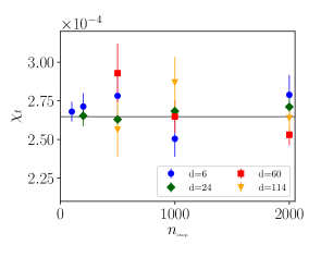
(a) $N=21$, $\beta_{L}=0.7$, $L=114$.

(b) $N=41$, $\beta_{L}=0.65$, $L=132$.

Figure 1: Topological susceptibility for various values of $n_{\mbox{\tiny step}}$ and $d$, compared to the result of  [9] obtained with 11 (left) and 15 (right) replicas.

One of the goals of this study is to understand the magnitude of the numerical effort needed, in terms of out-of-equilibrium evolutions, in order to sample efficiently a system with PBC, starting from a system with a defect or with full OBC. To that aim, we display in Figs. 2(a) and 2(b) the values of the Effective Sample Size as a function of $d$ (left panel) and $n_{\mbox{\tiny step}}$ (right panel). Qualitatively speaking, a very small ESS (e.g., $<0.05$) signals a (possibly extremely) inefficient sampling of the target distribution. Visual inspection of Fig. 2(a) shows that the ESS is a decreasing function of the defect length $d$. This is in agreement with the fact that a prior system defined by larger defect length $d$ is farther from the target one with PBC. Thus, at a fixed value of $n_{\mbox{\tiny step}}$, sampling a system with PBC is increasingly more difficult as the prior system approaches the full OBC (embodied by the choice $d=L$). At the same time, as can be seen from Fig. 2(b), ESS is an increasing function of $n_{\mbox{\tiny step}}$. Hence, a simple solution to this issue seems to be to increase $n_{\mbox{\tiny step}}$ to a sufficiently large value for each $d$. Intuitively, this makes the evolution slower, as it is close to a quasi-equilibrium evolution, and also more expensive to perform.

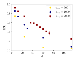
(a) ESS as a function of the length $d$ of the defect.

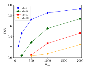
(b) ESS as a function of the number of steps in each evolution.

Figure 2: ESS for different combinations of lengths of the defect and total number of steps in each evolution, for $N=21$, $\beta_{L}=0.7$ and $L=114$..

Finally, we display in Figs. 3(a) and 3(b) preliminary results concerning the efficiency of this method compared to the PTBC approach. We compare the error on the quantity $\chi_{t}$, multiplied by the square root of the total numerical effort spent to obtain the numerical results. In the case of the out-of-equilibrium evolutions, this is given by $(n_{\mbox{\tiny step}}+n_{\mbox{\tiny relax}})\times n_{\mbox{\tiny ev}}$, while in case of the PTBC algorithm this is given by the number of measurements multiplied by the number of replicas. No specific choice in terms of the values of $n_{\mbox{\tiny step}}$ or $d$ seems to be strikingly more efficient than others. Moreover, it is quite encouraging to see that even for large values of $d$, non-equilibrium methods provide remarkably competitive results, although the computational cost in terms of updates per evolution is larger. Generally speaking, non-equilibrium evolutions performed with $n_{\mbox{\tiny step}}=1000$ or $2000$ enable a very precise sampling of the target distribution, even if the number of evolutions $n_{\mbox{\tiny ev}}$ themselves is comparably smaller. This is not surprising, as the use of relatively large values of $n_{\mbox{\tiny step}}$ was essentially the same strategy already followed in the computation of the $\mathrm{SU}(3)$ equation of state in Ref. [20].

(a) $N=21$, $\beta_{L}=0.7$, $L=114$.

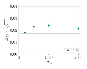
(b) $N=41$, $\beta_{L}=0.65$, $L=132$.

Figure 3: Efficiency in the computation of $\chi_{t}$ for various values of $n_{\mbox{\tiny step}}$ and $d$, compared to the parallel tempering (black band) from [9].

In the case of $N=21$, displayed in Fig. 3(a), the preliminary results for out-of-equilibrium evolutions presented in this contribution are not yet comparable in efficiency with PTBC: we remark however that we opted for a very conservative estimation of the errors. In this respect, results obtained for $N=41$ shown in Fig. 3(b) are even more encouraging, since autocorrelation times grow as a function of $N$, making topological freezing much worse at larger values of $N$.

4 Conclusions and future outlooks

In this contribution we showcased the first application of out-of-equilibrium methods based on Jarzynski’s equality towards the mitigation of so-called freezing of topological observables in lattice field theory.

With this method, it is possible to leverage the milder autocorrelation times that enjoyed by lattice models with open boundary conditions while simultaneously bypassing the complications they introduce. With an exact reweighting-like method, the physically-interesting observables with periodic boundaries could be computed, and the preliminary numerical results on the $2d$ $\mathrm{CP}^{N-1}$ models show that this method is already competitive with state-of-the-art calculations performed with the PTBC algorithm, an approach that has recently seen wide use also for non-Abelian gauge theories in four dimensions.

An advantage of out-of-equilibrium evolutions over PTBC is that no additional replicas are needed, as each evolution is simulated independently. Moreover, as shown by recent studies on Stochastic Normalizing Flows (SNFs), the combination of non-equilibrium methods with the coupling layers of Normalizing Flows allows to improve their efficiency even further. This opens up to a potentially exciting new development for the algorithmic approach pioneered in the present study, as a suitable training process of only moderate length could provide the values of the parameters of the coupling layers of SNFs. In the future, we plan to explore this direction by implementing the above method with a suitable SNF architecture. This could boost even further its numerical efficiency, and provide a unique approach to mitigate topological freezing in the $2d$ $\mathrm{CP}^{N-1}$ models, and beyond.

References

- [1] B. Alles, G. Boyd, M. D’Elia, A. Di Giacomo and E. Vicari, Hybrid Monte Carlo and topological modes of full QCD, Phys. Lett. B 389 (1996) 107 [hep-lat/9607049].
- [2] P. de Forcrand, M. Garcia Perez, J. E. Hetrick and I.-O. Stamatescu, Topology of full QCD, Nucl. Phys. Proc. Suppl. 63 (1998) 549 [hep-lat/9710001].
- [3] B. Lucini and M. Teper, gauge theories in four-dimensions: Exploring the approach to , JHEP 06 (2001) 050 [hep-lat/0103027].
- [4] L. Del Debbio, H. Panagopoulos and E. Vicari, dependence of gauge theories, JHEP 08 (2002) 044 [hep-th/0204125].
- [5] D. B. Leinweber, A. G. Williams, J.-b. Zhang and F. X. Lee, Topological charge barrier in the Markov chain of QCD, Phys. Lett. B 585 (2004) 187 [hep-lat/0312035].
- [6] L. Del Debbio, G. M. Manca and E. Vicari, Critical slowing down of topological modes, Phys. Lett. B 594 (2004) 315 [hep-lat/0403001].
- [7] C. Bonati and M. D’Elia, Topological critical slowing down: variations on a toy model, Phys. Rev. E 98 (2018) 013308 [1709.10034].
- [8] C. Bonanno, C. Bonati and M. D’Elia, Topological properties of models in the large- limit, JHEP 01 (2019) 003 [1807.11357].
- [9] M. Berni, C. Bonanno and M. D’Elia, Large- expansion and -dependence of models beyond the leading order, Phys. Rev. D 100 (2019) 114509 [1911.03384].
- [10] C. Bonanno, C. Bonati and M. D’Elia, Large- Yang-Mills theories with milder topological freezing, JHEP 03 (2021) 111 [2012.14000].
- [11] A. Athenodorou and M. Teper, SU(N) gauge theories in 3+1 dimensions: glueball spectrum, string tensions and topology, JHEP 12 (2021) 082 [2106.00364].
- [12] Bennett, D. K. Hong, J.-W. Lee, C. J. D. Lin, B. Lucini, M. Piai et al., Sp(2N) Yang-Mills theories on the lattice: Scale setting and topology, Phys. Rev. D 106 (2022) 094503 [2205.09364].
- [13] C. Bonanno, M. D’Elia, B. Lucini and D. Vadacchino, Towards glueball masses of large-N SU(N) pure-gauge theories without topological freezing, Phys. Lett. B 833 (2022) 137281 [2205.06190].
- [14] C. Bonanno, Lattice determination of the topological susceptibility slope of CPN-1 models at large , Phys. Rev. D 107 (2023) 014514 [2212.02330].
- [15] M. Lüscher and S. Schaefer, Lattice QCD without topology barriers, JHEP 07 (2011) 036 [1105.4749].
- [16] M. Lüscher and S. Schaefer, Lattice QCD with open boundary conditions and twisted-mass reweighting, Comput. Phys. Commun. 184 (2013) 519 [1206.2809].
- [17] M. Hasenbusch, Fighting topological freezing in the two-dimensional model, Phys. Rev. D 96 (2017) 054504 [1706.04443].
- [18] C. Jarzynski, Nonequilibrium Equality for Free Energy Differences, Phys. Rev. Lett. 78 (1997) 2690 [cond-mat/9610209].
- [19] M. Caselle, G. Costagliola, A. Nada, M. Panero and A. Toniato, Jarzynski’s theorem for lattice gauge theory, Phys. Rev. D 94 (2016) 034503 [1604.05544].
- [20] M. Caselle, A. Nada and M. Panero, QCD thermodynamics from lattice calculations with nonequilibrium methods: The SU(3) equation of state, Phys. Rev. D 98 (2018) 054513 [1801.03110].
- [21] O. Francesconi, M. Panero and D. Preti, Strong coupling from non-equilibrium Monte Carlo simulations, JHEP 07 (2020) 233 [2003.13734].
- [22] A. Bulgarelli and M. Panero, Entanglement entropy from non-equilibrium Monte Carlo simulations, JHEP 06 (2023) 030 [2304.03311].
- [23] G. Papamakarios, E. T. Nalisnick, D. J. Rezende, S. Mohamed and B. Lakshminarayanan, Normalizing flows for probabilistic modeling and inference, J. Mach. Learn. Res. 22 (2021) 1.
- [24] M. S. Albergo, D. Boyda, D. C. Hackett, G. Kanwar, K. Cranmer, S. Racanière et al., Introduction to Normalizing Flows for Lattice Field Theory, 2101.08176.
- [25] H. Wu, J. Köhler and F. Noé, Stochastic normalizing flows, Advances in Neural Information Processing Systems 33 (2020) 5933.
- [26] M. Caselle, E. Cellini, A. Nada and M. Panero, Stochastic normalizing flows as non-equilibrium transformations, JHEP 07 (2022) 015 [2201.08862].