Can bin-wise scaling improve consistency and adaptivity
of prediction uncertainty for machine learning regression ?

Abstract

Binwise Variance Scaling (BVS) has recently been proposed as a post hoc recalibration method for prediction uncertainties of machine learning regression problems that is able of more efficient corrections than uniform variance (or temperature) scaling. The original version of BVS uses uncertainty-based binning, which is aimed to improve calibration conditionally on uncertainty, i.e. consistency. I explore here several adaptations of BVS, in particular with alternative loss functions and a binning scheme based on an input-feature ($X$) in order to improve adaptivity, i.e. calibration conditional on X. The performances of BVS and its proposed variants are tested on a benchmark dataset for the prediction of atomization energies and compared to the results of isotonic regression.

I Introduction

Post hoc recalibration of machine learned (ML) prediction uncertainty for regression problems is currently an essential step to increase the reliability of uncertainty quantification (UQ)(Tran2020, ). Post hoc recalibration methods include, for instance, temperature scaling(Guo2017, ; Kuleshov2018, ; Levi2022, ), isotonic regression(Busk2022, ) and conformal inference(Angelopoulos2021, ; Hu2022, ). These methods focus either on average calibration or on consistency (i.e. calibration conditional on uncertainty)(Pernot2023c_arXiv, ). Until now, adaptivity, i.e. calibration conditional on input features(Angelopoulos2021, ), has surprisingly been left out of the frame of post hoc ML-UQ, despite its essential role in UQ reliability for the end user(Reiher2022, ; Pernot2023c_arXiv, ). It is important to stress out that prediction uncertainties with a perfect consistency are not necessarily reliable across the range of input features(Pernot2023_Arxiv, ). Consistency and adaptivity are two facets of calibration that should be simultaneously validated in order to approach the reliability of individual predictions.

Recently, a post hoc recalibration method based on binwise variance scaling (BVS) has been proposed by Frenkel and Goldberger(Frenkel2023, ), adapted from a similar method for classification problems(Frenkel2021, ). In this approach, a set of prediction uncertainties of size $M$ is sorted and split into $N$ equal-size bins. For each bin, a local uncertainty scaling factor is estimated to ensure calibration. These scaling factors are then applied to newly predicted uncertainties. In this setup based on uncertainty binning, the BVS approach aims to improve consistency. Indeed, BVS has been shown to perform better than uniform variance scaling for medical images regression tasks on the basis of consistency metrics (ENCE, UCE)(Frenkel2023, ).

In this short study I try to check if BVS can be used to improve both consistency and adaptivity beyond the trivial effect of average calibration. The next section (Sect. II) presents the BVS method, alternative loss functions and the scores or calibration metrics used to evaluate their performances. Application to the QM9 dataset of atomization energies is presented in Sect. III, leading to the discussion of the results and conclusions in Sect. IV.

II Methods

Frenkel and Goldberger(Frenkel2023, ) describe two approaches to BVS estimation. One is based on the equality of mean squared errors with mean squared uncertainty, and the other is based on the maximum likelihood solution, which is consistent with the z-scores based approach favored in my earlier studies.(Pernot2022b, ; Pernot2023c_arXiv, ) As both approach appear to produce similar results, I focus here on the second one.

II.1 Z-scores based BVS

Let us consider a set of $M$ prediction errors and uncertainties $\left\{E_{i},u_{i}\right\}_{i=1}^{M}$. The dataset is ordered by increasing uncertainty values and split into $N_{B}$ equal-size bins $B_{1},\ldots,B_{N_{B}}$. The local calibration within bin $i$ can be assessed by the $z$-scores mean square (ZMS)(Pernot2023c_arXiv, ), that should be equal to 1, i.e.

$$v_{i}=<Z_{j}^{2}>_{j\in B_{i}}=1$$ (1)

where $Z_{j}=E_{j}/u_{j}$.

A corrective scaling factor is thoroughly obtained as

$$s_{i}=v_{i}^{-1/2}$$ (2)

to be applied to uncertainties falling within the limits of the corresponding bin

$$u_{j\in B_{i}}\rightarrow u_{s,j\in B_{i}}=s_{i}u_{j\in B_{i}}$$ (3)

where $u_{s}$ denotes the scaled uncertainty.

The use of $u$ as a binning variable is adapted to improve consistency, but other variables can be used to target adaptivity, as shown below.

How many bins ?

BVS is typically based on an equal-size binning scheme, but the optimal bin number has to be defined. Reduction of the bin number to $N_{B}=1$ leads to the so-called temperature scaling method(Guo2017, ). Temperature scaling is able to ensure average calibration but not consistency.(Pernot2017, ; Pernot2017b, ; Pernot2022a, ) At the opposite, using one scaling factor per data point, $N_{B}=M$, leads to the singular solution $u_{s,j}=|E_{j}|$, the so-called oracle used in confidence curves(Pernot2022c, ). This scheme is useless, as having null-width intervals it cannot be applied to unseen uncertainties. In their applications, Frenkel and Goldberger(Frenkel2023, ) used $N_{B}=15$ without further justification. One might want to use more bins to account for possible small-scale consistency/adaptivity defects, but care has to be taken about over-parameterization. As BVS is a fast method, a systematic study over a wide range of bin numbers can be designed to orient the choice of the best $N_{B}$ value (Sect. III.2).

II.2 Score functions

Score functions are used to estimate the effect of scaling on the quality of the resulting uncertainties, but also to enable the estimation of optimal scaling factors by minimization of adapted loss functions.

Scores based on local statistics are based on a binning scheme which is independent of the BVS binning scheme. In the following, I use a partition of the binning variables into $N_{S}$ equal-size bins, $B_{S,1},\ldots,B_{S,N_{S}}$. Other partitions have been considered (e.g. adaptive binning based on equal-with bins, see Appendix B in Ref. (Pernot2023_Arxiv, )), but they do not bring any notable improvement to the results presented below.

II.2.1 Score functions based on mean squared z-scores

Scores are defined to measure the closeness of the z-scores mean squares (ZMS) to 1. For average calibration, one defines

$$S_{cal}=|\ln<Z^{2}>|$$ (4)

where the average is taken over the full dataset. The logarithm accounts for the fact that we are considering a scale statistic (a ZMS of 2 entails a correction of the same amplitude as a ZMS of 0.5). For perfect average calibration, one should have $S_{cal}=0$.

Similarly, one can define a mean calibration error

$$S_{x}=\frac{1}{N_{S}}\sum_{i=1}^{N_{S}}|\ln<Z_{j}^{2}>_{j\in B_{S,i}}|$$ (5)

where $i$ runs over the $N_{S}$ bins and $x$ is the variable used to define those bins. $S_{x}$ has to be as small as possible but cannot be expected to reach 0 (see Sect. II.3 for the estimation of a target value).

A combination of the $S_{x}$ scores can be used to design loss functions in order to achieve specific goals. For instance, consistency can be targeted by minimizing

$$S_{con}=S_{cal}+S_{u}$$ (6)

while adaptivity can be targeted with

$$S_{ada}=S_{cal}+\sum S_{X_{i}}$$ (7)

where $X_{i}$ is an input feature or an adequate proxy. The combination of all these scores

$$S_{tot}=S_{cal}+S_{u}+\sum S_{X_{i}}$$ (8)

measures consistency and adaptivity. Note that $S_{cal}$ is always included, as it is a basic requirement for proper calibration.

II.2.2 Negative Log Likelihood

Another option to optimize the BVS factors is to minimize the average negative log likelihood function (NLL)(Frenkel2023, )

$$NLL =\frac{1}{2M}\sum_{i=1}^{M}\left(\frac{E_{i}^{2}}{u_{i}^{2}}+\ln u_{i}^{2}+\ln 2\pi\right)$$ (9)

$$=\frac{1}{2}\left(<Z^{2}>+<\ln u^{2}>+\ln 2\pi\right)$$ (10)

which combines an average calibration term based on the mean squared z-scores, and a sharpness term driving the uncertainties towards small values(Gneiting2007a, ), hence preventing the minimization of $<Z^{2}>$ by arbitrary large uncertainties. Frenkel and Goldberger(Frenkel2023, ) have shown that the scaling factors defined in Eq. 2 minimize the NLL.

II.2.3 ENCE

For reference, let us consider also a statistic used by Frenkel and Goldberger(Frenkel2023, ), namely the Expected Normalized Calibration Error

$$ENCE=\frac{1}{N_{S}}\sum_{i=1}^{N_{S}}\frac{|MV_{i}^{1/2}-MSE_{i}^{1/2}|}{MV_{i}^{1/2}}$$ (11)

where $MV_{i}=\frac{1}{|B_{S,i}|}\sum_{j\in B_{S,i}}u_{j}^{2}$ and $MSE_{i}=\frac{1}{|B_{S,i}|}\sum_{j\in B_{S,i}}E_{j}^{2}$. It expresses the calibration error as a percentage and should be as close to 0 as possible. A specific target value is defined below.

Similarly to the $S_{x}$ scores, one can define $ENCE_{u}$ as a consistency metric and $ENCE_{X_{i}}$ as adaptivity metric(s) by using adapted binning schemes. Note that the extension of mean calibration error to alternative binning schemes is being used in the literature to measure adversarial calibration(Chung2021, ).

II.3 Target values for the NLL, $S_{x}$ and $ENCE_{x}$ scores

For a given dataset, the best values reachable by statistics such as the $S_{x}$ or ENCE are not 0, as they result from the mean of a sample of positive values. For an illustration about ENCE, see for instance Pernot(Pernot2023a_arXiv, ). The optimal value depends on the size of the dataset and on $N_{S}$. In order to get an estimation, one needs a dataset offering compatibility between errors and uncertainties. As one cannot easily infer perfect uncertainties, one has to generate pseudo-errors from the available uncertainties, using for instance a zero-centered normal distribution: $\tilde{E_{i}}\sim N(0,u_{i})$ and calculate the scores using $\tilde{E}$ and $u$. Sampling a large number (e.g. $10^{3}$) of such generated datasets provides an estimate of the optimal score values and of their uncertainties.(Pernot2022c, ; Rasmussen2023, ) These values are denoted as simulated (“Simul”) in the following.

It has to be noted that for the NLL the simulated value is not necessarily smaller than the actual values because the data are modified. In this case, one has thus to consider the amplitude of the difference between the actual NLL and its simulated value.(Rasmussen2023, )

II.4 Validation metrics

The scores presented above enable to compare between methods but do not directly enable to validate calibration. Estimation of confidence intervals (CI) on the local ZMS values provides the basis for a validation metric(Pernot2022a, ; Pernot2023c_arXiv, ): for a perfectly calibrated dataset, the fraction of binned statistics with a confidence interval containing the target value should be close to the coverage probability of the CIs. Namely, about 95 % of the local ZMS values should have their 95 % CI containing the target value. Let us denote this fraction of “valid” intervals by $f_{v}$. In practice, one should not expect to recover exactly $f_{v}=0.95$, and a CI for $f_{v}$ has also to be estimated from the binomial distribution to account for the limited number of bins(Pernot2022a, ). The value of $f_{v}$ depends on the binning variable $x\in\left\{u,X_{i}\right\}$ and is indexed accordingly as $f_{v,x}$.

For a correct estimation of $f_{v,x}$, it is important to ensure a good balance between the bin size (estimation of local ZMS values and their CIs by bootstrapping, as described in Ref. (Pernot2023c_arXiv, )) and the number of bins (estimation of $f_{v,x}$ and its CI). Using a bin size of $M^{1/2}$ seems to be a rational choice(Watts2022, ), which might limit the use of $f_{v}$ to datasets with at least $10^{4}$ points. The 95 % CIs on local ZMS values are estimated by the BCa bootstrapping method(DiCiccio1996, ) with 1500 draws, and the number of bins is set to $N_{S}=100$.

III Results

To illustrate the methods presented above, I use a set of data produced and presented by J. Busk et al.(Busk2022, ). The QM9 dataset contains predicted atomization energies ($V$) and uncertainties ($u_{V}$), reference values ($R$), and molecular formulas as input feature. These data are transformed to $C=\left\{X_{1},X_{2},E=R-V,u=u_{V}\right\}$, where $X_{1}$ is the molecular mass and $X_{2}$ the fraction of hetero-atoms generated from the formulas(Pernot2023_Arxiv, ; Bakowies2021, ). $X_{1}$ and $X_{2}$ are used here as complementary proxies for the molecular formula.

In the original study, the uncertainties were recalibrated by isotonic regression(Busk2022, ) and were later shown to reach a good consistency while having adaptivity problems(Pernot2023c_arXiv, ). It is not pertinent to test BVS on these transformed data (mostly because of the stratification induced by isotonic regression)(Pernot2023b_arXiv, ), and J. Busk kindly provided me with the validation set ($M=10000$) and test set ($M=13885$) of uncalibrated predictions used for their isotonic regression study. It has to be noted that the $X_{1}$ and $X_{2}$ variables are stratified, i.e. they achieve a finite number of values over which the data points are distributed. This can have an impact when they are used to define bins(Pernot2023b_arXiv, ).

This datasets enable the direct comparison of BVS and isotonic regression performances. BVS factors are estimated on the validation set (denoted below as training set) and their transferability is assessed on the test set. Optimization of scaling factors provided by Eq. 2 was attempted for $u$- and $X_{1}$-based binning schemes and for the NLL, $S_{tot}$, $S_{con}$ and $S_{ada}$ loss functions. In all the cases, the scaling factors were initialized by Eq. 2 and optimized by a global optimizer, followed by a local optimizer until convergence. When the score of the optimized solution did not improve on the initial values (as expected for the NLL loss), the latter were kept as the optimum.

III.1 Unscaled data

Average calibration of the training set is assessed by comparing the ZMS to 1. One gets $<Z^{2}>=0.31(1)$, revealing a mismatch between errors and uncertainties. This corresponds to the calibration score $S_{cal}=1.17$ in Table 1. Similar values are obtained for the test set ($<Z^{2}>=0.32(1)$, $S_{cal}=1.13$). These $S_{cal}$ values have to be compared to their simulated target, 0. The other scores for both uncalibrated sets are also comparable. Globally, the datasets are not biased, with $<Z>\leq 0.02$.

It is always possible to correct average calibration by a uniform scaling of the uncertainties, but if one wants to reach consistency, the uncertainties need to have some level of positive correlation with the errors. This can be checked by plotting a confidence curve, displaying the RMS of error sets iteratively pruned from the points with the largest uncertainties.(Pernot2022b, ; Pernot2022c, ) Note that confidence curves are insensitive to the scale of errors and uncertainties. A continuously decreasing curve reveals a sane situation where large errors are associated with large uncertainties, and where one might hope to improve the situation with post-hoc calibration. This is the case for the studied datasets [Fig. 1(a)], for which the confidence curves show a sharp fall-off followed by a continuous decrease. The sharp feature at the beginning shows that the largest uncertainties are correctly associated to very large errors.

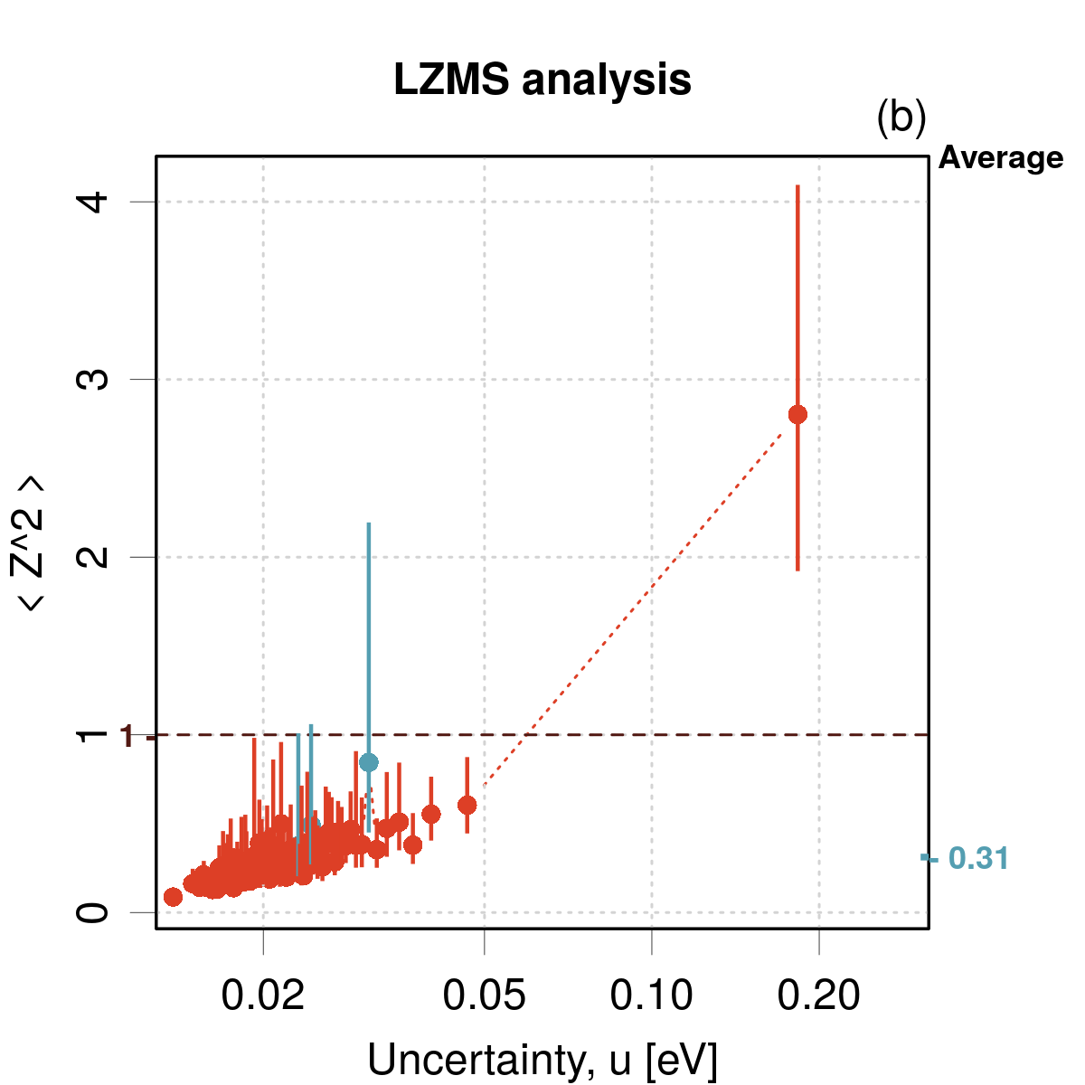
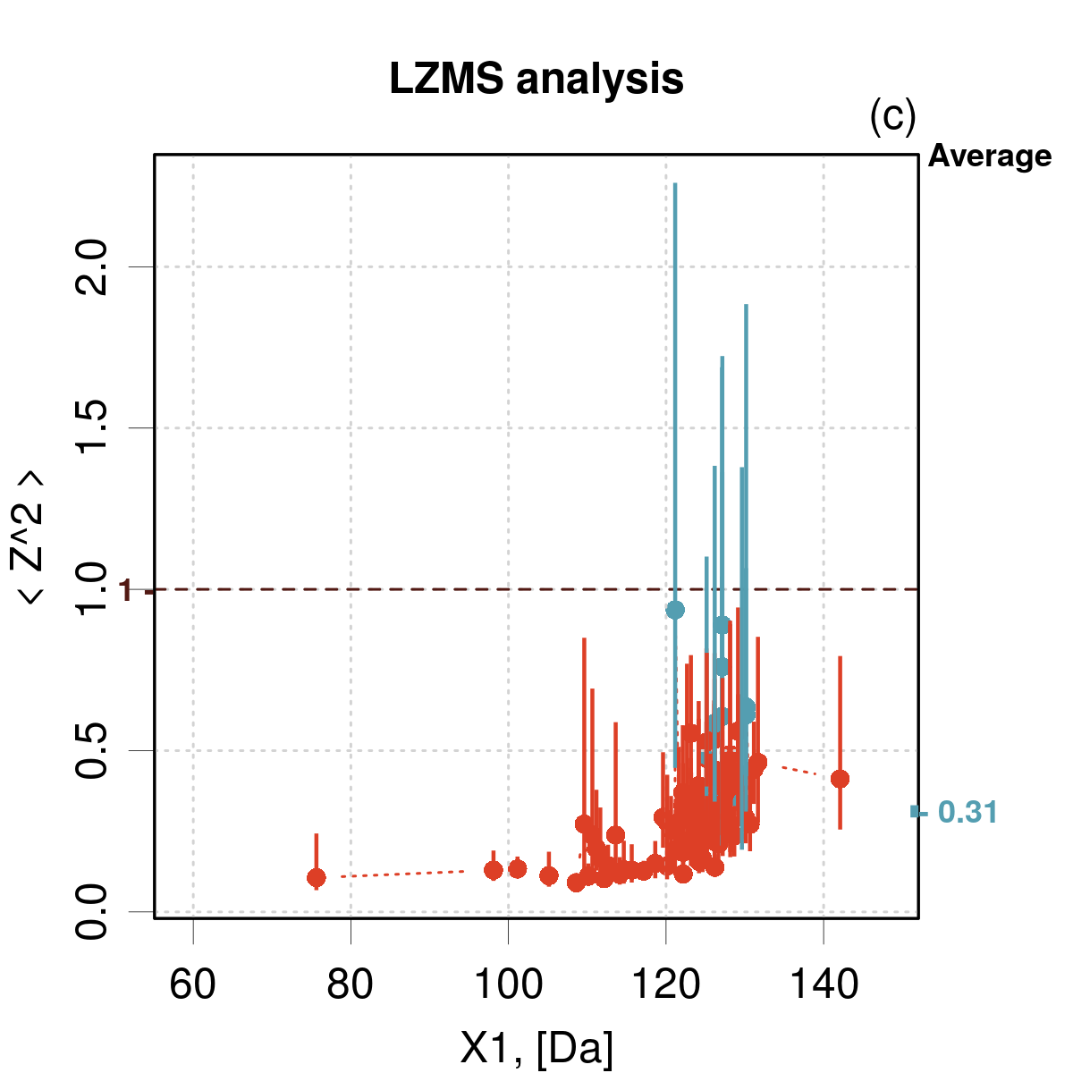
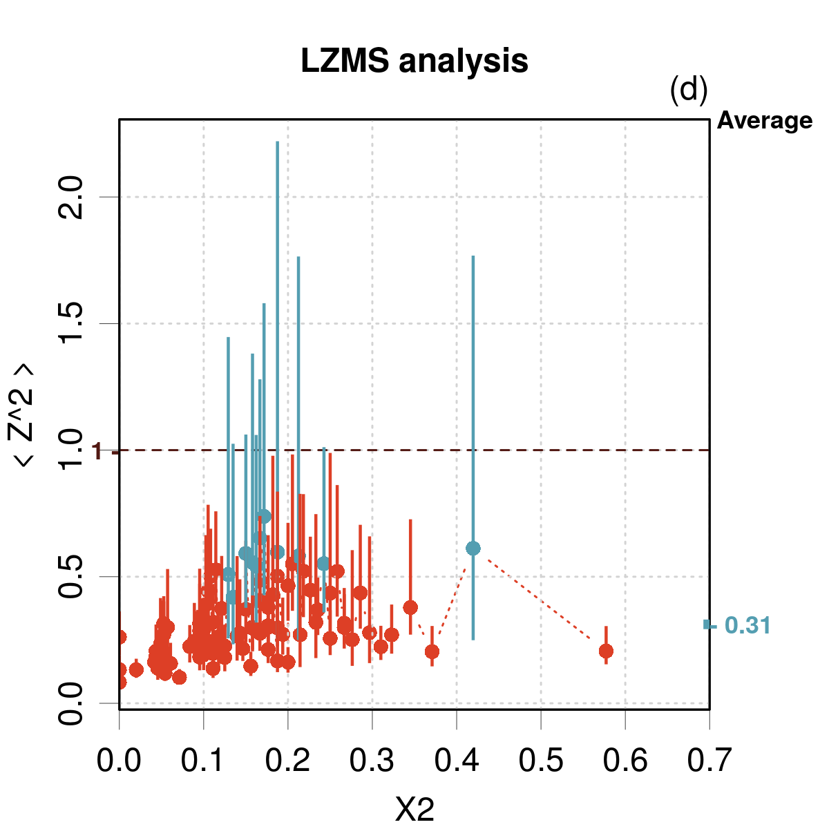
Figure 1: Analysis of the unscaled datasets: (a) confidence curves for the training and test sets; (b-d) LZMS analysis for the training set against $u$, $X_{1}$ and $X_{2}$ (the red intervals do not contain the target value).

Consistency can be assessed on a local Z-mean-squares (LZMS) plot(Pernot2023c_arXiv, ) [Fig. 1(b)]. The positive slope of the LZMS values as a function of $u$ shows that a uniform scaling will not be sufficient to bring all the CIs to enclose the $<Z^{2}>=1$ line. The outlying point at high uncertainty corresponds to the sharp feature observed in the confidence curve. The LZMS analysis shows also that a monotonous scaling (linear or isotonic) can probably be effective to restore consistency (as shown by Busk et al. (Busk2022, )). The LZMS plot for the test set is very similar (not shown). Analysis of adaptivity by LZMS plots against $X_{1}$ and $X_{2}$ [Fig. 1(c-d)] does not present the regularity observed for the consistency analysis. The LZMS statistics are more locally dispersed, and it is clear that a uniform or linear scaling of $u$ has little chance to be fully efficient.

III.2 Optimal BVS binning

The performance of the BVS scores resulting from Eq. 2 was assessed on the test set for a range of bin numbers between 2 and 99, and compared to the results of isotonic regression and simulated datasets (Fig. 2).

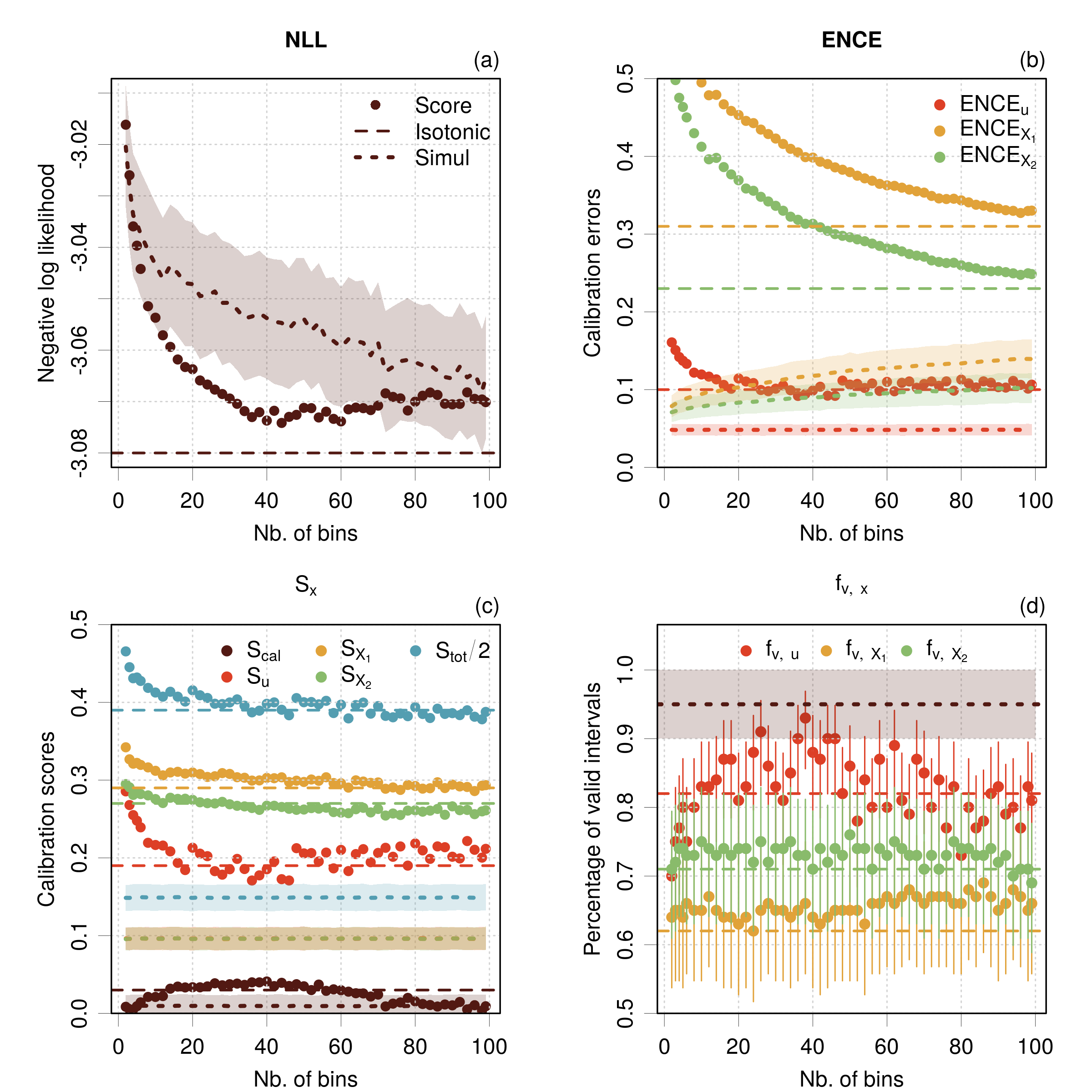
Figure 2: Dependence of the BVS scores on the test set with the number of bins. The dashed horizontal lines depict the values for isotonic regression and the dotted lines the values for simulated datasets. The gray area in panel (d) corresponds to a 95 % CI on the $f_{v,x}$ values for simulated data. $S_{tot}$ and its isotonic and simulated references are scaled by a factor 0.5 for legibility.

The NLL value [Fig. 2(a)] decreases monotonously with increasing bin numbers up to about 40, after which, it starts a slow noisy rise. It never crosses the isotonic regression reference line. In contrast, the line for simulated datasets follows a monotonous decrease. The difference between the actual NLL curve and the simulated one results from a misfit of average calibration, which starts at 0 for a single bin, reaches a maximum around 40 bins and decreases again. This feature can be observed through the $S_{cal}$ score in [Fig. 2(c)]. As they share the same uncertainty set, the sharpness contribution is identical for both curves, and it parallels the simulated NLL curve. Note that the minimum in the NLL curve should not be interpreted as an optimum for the number of bins: it points a contrario to an area with poor calibration performances. The areas at low and large bin numbers where the NLL curve overlaps the simulated CI are those where the average calibration of the scaled test set is at its best.

The $ENCE_{x}$ statistics are shown in [Fig. 2(b)]. $ENCE_{u}$ decreases down to $\sim$0.1 at about 40 bins after which it increases slightly to reach a plateau. At its minimum, it is slightly lower than the corresponding isotonic regression reference, while the plateau is slightly above this value. The ENCE curves for the other binning variables present a steady decrease over the studied bin range and they do not reach their isotonic regression reference. In contrast to the NLL, the three $ENCE_{x}$ curves stray far above their simulated values.

If one considers the $S_{x}$ statistics [Fig. 2(c)], the $S_{u}$ curve parallels perfectly the $ENCE_{u}$ curve. The $S_{X_{2}}$ curve presents a shallow minimum around 70 bins, and it gets lower than the isotonic regression value at about 40 bins. The $S_{X_{1}}$ curve presents no minimum in the studied range. It reaches the corresponding isotonic value near 70 bins. None of these scores reaches the simulated values (all identical at about 0.1). Contrasting with the other scores, $S_{cal}$ increases up to around 40 bins before decreasing. It exceeds the isotonic regression value between 15 and 60 bins. As for the NLL curve, the $S_{cal}$ curve matches its simulated reference at small and large bin numbers. This behavior reflects the fact that the scaling of individual bins by BVS cannot guarantee average calibration for the test set. The $S_{tot}$ score combines the four previous $S_{x}$ scores and shows a decrease up to 70 bins followed by a plateau. The isotonic regression reference is reached for about 40 bins. $S_{tot}$ is dominated by adaptivity errors and does never match its simulated reference.

Fig. 2(d) presents the $f_{v,x}$ validation statistics with their confidence intervals. A shaded area depicts the 95 % CI for the simulated datasets, identical for all three statistics. Globally, considering the uncertainties on the statistics, there is no noticeable departure of BVS statistics from the isotonic regression ones, except maybe for $f_{v,u}$ between 30 and 50 bins, where it gets closer to the 0.95 target and the simulated values. This comforts the diagnostic that choosing $N_{B}=40$ would be the best option to ensure consistency with NLL scaling factors.

This preliminary analysis leaves us with mixed messages: (i) it is noticeable that most statistics are noisy and that a slight change in bin number might affect the performance, notably when comparing to the isotonic regression reference; (ii) if one wants to achieve good consistency, the $ENCE_{u}$ and $S_{u}$ scores agree that one should not use more than 20-40 bins, and in favorable cases Eq. 2 can perform slightly better than isotonic regression; (iii) to consistently equal or outperform isotonic regression on adaptivity scores, one needs at least 50, and up to 80 bins. In any case, these scaling factors do not seem to be able to achieve simultaneously consistency and adaptivity.

However, these results do not augur of the performances of scaling factors optimized with loss functions other than the NLL. A range of options for alternative scaling factors will be tested in the following for $N_{B}=20$, 40 and 80 bins.

III.3 BVS performance

In this section, scaling factors based on loss functions other than the NLL, i.e. $S_{tot}$, $S_{con}$ and $S_{ada}$, are estimated and compared to the results of isotonic regression and simulated data. The results for $N_{B}=20$, 40 and 80 are provided in Tables 1, 2 and 3, respectively.

I do not discuss the overall improvement brought by all scaling scenarios, which is a trivial effect due to the improvement of average calibration, and mostly focus on smaller scale effects related to consistency and adaptivity.

Binning	Dataset	Scaling		NLL$\downarrow$			$S_{cal}\downarrow$		$S_{u}\downarrow$		$S_{X_{1}}\downarrow$		$S_{X_{2}}\downarrow$		$S_{tot}\downarrow$			$f_{v,u_{E}}$		$f_{v,X_{1}}$		$f_{v,X_{2}}$
	Training	No		-2.	76		1.	17	1.	32	1.	29	1.	27	5.	04		[0.	01, 0.09]	[0.	04, 0.17]	[0.	07, 0.20]
	Test	No		-2.	75		1.	13	1.	39	1.	27	1.	27	5.	06		[0.	01, 0.09]	[0.	09, 0.24]	[0.	06, 0.19]
		Isotonic		-3.	08		0.	03	0.	19	0.	29	0.	27	0.	78		[0.	73, 0.89]	[0.	52, 0.71]	[0.	61, 0.79]
		Simul		-			0.	00	0.	10	0.	09	0.	09	0.	29		[0.	90,1.00]	[0.	90,1.00]	[0.	90,1.00]
$u$	Training	NLL		-3.	05		0.	00	0.	21	0.	33	0.	29	0.	83		[0.	78, 0.93]	[0.	56, 0.75]	[0.	65, 0.83]
		$S_{tot}$		-3.	05		0.	00	0.	19	0.	33	0.	29	0.	81		[0.	78, 0.93]	[0.	56, 0.75]	[0.	65, 0.83]
		$S_{con}$		-3.	05		0.	00	0.	18	0.	33	0.	29	0.	80		[0.	81, 0.94]	[0.	56, 0.75]	[0.	66, 0.84]
		$S_{ada}$		-3.	05		0.	00	0.	21	0.	33	0.	29	0.	82		[0.	80, 0.93]	[0.	56, 0.75]	[0.	65, 0.83]
	Test	NLL		-3.	06		0.	03	0.	21	0.	31	0.	27	0.	83		[0.	72, 0.88]	[0.	53, 0.72]	[0.	64, 0.82]
		$S_{tot}$		-3.	06		0.	03	0.	20	0.	31	0.	27	0.	82		[0.	78, 0.93]	[0.	53, 0.72]	[0.	64, 0.82]
		$S_{con}$		-3.	06		0.	03	0.	20	0.	31	0.	27	0.	81		[0.	75, 0.90]	[0.	53, 0.72]	[0.	65, 0.83]
		$S_{ada}$		-3.	06		0.	03	0.	20	0.	31	0.	28	0.	82		[0.	75, 0.90]	[0.	53, 0.72]	[0.	63, 0.81]
$X_{1}$	Training	NLL		-3.	03		0.	00	0.	28	0.	27	0.	32	0.	87		[0.	60, 0.79]	[0.	66, 0.84]	[0.	63, 0.81]
		$S_{tot}$		-3.	03		0.	00	0.	24	0.	27	0.	32	0.	83		[0.	67, 0.85]	[0.	65, 0.83]	[0.	62, 0.80]
		$S_{con}$		-3.	03		0.	00	0.	24	0.	28	0.	32	0.	83		[0.	69, 0.86]	[0.	67, 0.85]	[0.	62, 0.80]
		$S_{ada}$		-3.	03		0.	00	0.	28	0.	28	0.	31	0.	87		[0.	64, 0.82]	[0.	67, 0.85]	[0.	63, 0.81]
	Test	NLL		-2.	98		0.	08	0.	33	0.	35	0.	37	1.	13		[0.	52, 0.71]	[0.	51, 0.70]	[0.	52, 0.71]
		$S_{tot}$		-2.	98		0.	08	0.	34	0.	35	0.	37	1.	13		[0.	49, 0.69]	[0.	53, 0.72]	[0.	51, 0.70]
		$S_{con}$		-2.	98		0.	08	0.	33	0.	35	0.	37	1.	13		[0.	53, 0.72]	[0.	51, 0.70]	[0.	52, 0.71]
		$S_{ada}$		-2.	98		0.	08	0.	32	0.	34	0.	37	1.	10		[0.	53, 0.72]	[0.	51, 0.70]	[0.	52, 0.71]
$u\,\&\,X_{1}$	Training	NLL		-3.	12		0.	00	0.	11	0.	14	0.	17	0.	42		[0.	87, 0.98]	[0.	81, 0.94]	[0.	78, 0.93]
	Test			-3.	03		0.	17	0.	27	0.	24	0.	25	0.	93		[0.	63, 0.81]	[0.	61, 0.79]	[0.	58, 0.77]
OxNy	Training	NLL		-3.	03		0.	00	0.	30	0.	31	0.	24	0.	85		[0.	59, 0.78]	[0.	69, 0.86]	[0.	77, 0.92]
groups	Test			-3.	01		0.	04	0.	28	0.	32	0.	26	0.	91		[0.	58, 0.77]	[0.	65, 0.83]	[0.	68, 0.85]

Table 1: Scores and validation metrics for various scaling schemes with $N_{B}=20$. Bold values denote the best scores within a group delimited by horizontal rules for the scores, and the intervals containing the 95 % target for the $f_{v}$ statistics. The statistics for isotonic regression are generated from the results of Busk et al. (Busk2022, ). The “Simul” scores are obtained by averaging over simulated error sets with the same uncertainties as the training or test set.

Binning	Dataset	Scaling		NLL$\downarrow$			$S_{cal}\downarrow$		$S_{u}\downarrow$		$S_{X_{1}}\downarrow$		$S_{X_{2}}\downarrow$		$S_{tot}\downarrow$			$f_{v,u_{E}}$		$f_{v,X_{1}}$		$f_{v,X_{2}}$
	Training	No		-2.	76		1.	17	1.	32	1.	29	1.	27	5.	04		[0.	01, 0.09]	[0.	04, 0.17]	[0.	07, 0.20]
	Test	No		-2.	75		1.	13	1.	39	1.	27	1.	27	5.	06		[0.	01, 0.09]	[0.	09, 0.24]	[0.	06, 0.19]
		Isotonic		-3.	08		0.	03	0.	19	0.	29	0.	27	0.	78		[0.	73, 0.89]	[0.	52, 0.71]	[0.	61, 0.79]
		Simul		-			0.	00	0.	10	0.	09	0.	09	0.	29		[0.	90,1.00]	[0.	90,1.00]	[0.	90,1.00]
$u$	Training	NLL		-3.	05		0.	00	0.	16	0.	32	0.	28	0.	77		[0.	88, 0.98]	[0.	57, 0.76]	[0.	66, 0.84]
		$S_{tot}$		-3.	05		0.	00	0.	13	0.	32	0.	28	0.	73		[0.	89, 0.99]	[0.	56, 0.75]	[0.	66, 0.84]
		$S_{con}$		-3.	05		0.	00	0.	13	0.	32	0.	28	0.	73		[0.	87, 0.98]	[0.	57, 0.76]	[0.	66, 0.84]
		$S_{ada}$		-3.	05		0.	00	0.	17	0.	32	0.	28	0.	77		[0.	84, 0.96]	[0.	56, 0.75]	[0.	65, 0.83]
	Test	NLL		-3.	07		0.	04	0.	19	0.	30	0.	27	0.	80		[0.	80, 0.93]	[0.	54, 0.73]	[0.	61, 0.79]
		$S_{tot}$		-3.	07		0.	04	0.	19	0.	30	0.	27	0.	80		[0.	82, 0.95]	[0.	54, 0.73]	[0.	61, 0.79]
		$S_{con}$		-3.	07		0.	04	0.	18	0.	30	0.	27	0.	79		[0.	83, 0.96]	[0.	54, 0.73]	[0.	61, 0.79]
		$S_{ada}$		-3.	07		0.	04	0.	18	0.	30	0.	27	0.	79		[0.	82, 0.95]	[0.	55, 0.74]	[0.	61, 0.79]
$X_{1}$	Training	NLL		-3.	04		0.	00	0.	24	0.	24	0.	28	0.	76		[0.	72, 0.88]	[0.	73, 0.89]	[0.	65, 0.83]
		$S_{tot}$		-3.	04		0.	00	0.	21	0.	24	0.	28	0.	73		[0.	75, 0.90]	[0.	74, 0.90]	[0.	65, 0.83]
		$S_{con}$		-3.	04		0.	00	0.	20	0.	24	0.	28	0.	71		[0.	77, 0.92]	[0.	74, 0.90]	[0.	65, 0.83]
		$S_{ada}$		-3.	04		0.	00	0.	24	0.	24	0.	28	0.	76		[0.	71, 0.87]	[0.	74, 0.90]	[0.	66, 0.84]
	Test	NLL		-2.	98		0.	06	0.	30	0.	37	0.	38	1.	11		[0.	60, 0.79]	[0.	48, 0.68]	[0.	49, 0.69]
		$S_{tot}$		-2.	98		0.	06	0.	31	0.	37	0.	38	1.	12		[0.	61, 0.79]	[0.	47, 0.67]	[0.	51, 0.70]
		$S_{con}$		-2.	98		0.	06	0.	30	0.	37	0.	38	1.	11		[0.	61, 0.79]	[0.	49, 0.69]	[0.	50, 0.70]
		$S_{ada}$		-2.	98		0.	06	0.	30	0.	37	0.	38	1.	12		[0.	57, 0.76]	[0.	49, 0.69]	[0.	48, 0.68]

Table 2: Same as Table 1 for $N_{B}=40$.

Binning	Dataset	Scaling		NLL$\downarrow$			$S_{cal}\downarrow$		$S_{u}\downarrow$		$S_{X_{1}}\downarrow$		$S_{X_{2}}\downarrow$		$S_{tot}\downarrow$			$f_{v,u_{E}}$		$f_{v,X_{1}}$		$f_{v,X_{2}}$
	Training	No		-2.	76		1.	17	1.	32	1.	29	1.	27	5.	04		[0.	01, 0.09]	[0.	04, 0.17]	[0.	07, 0.20]
	Test	No		-2.	75		1.	13	1.	39	1.	27	1.	27	5.	06		[0.	01, 0.09]	[0.	09, 0.24]	[0.	06, 0.19]
		Isotonic		-3.	08		0.	03	0.	19	0.	29	0.	27	0.	78		[0.	73, 0.89]	[0.	52, 0.71]	[0.	61, 0.79]
		Simul		-			0.	00	0.	10	0.	09	0.	09	0.	29		[0.	90,1.00]	[0.	90,1.00]	[0.	90,1.00]
$u$	Training	NLL		-3.	06		0.	00	0.	13	0.	31	0.	27	0.	70		[0.	89, 0.99]	[0.	56, 0.75]	[0.	66, 0.84]
		$S_{tot}$		-3.	06		0.	00	0.	10	0.	30	0.	26	0.	66		[0.	89, 0.99]	[0.	59, 0.78]	[0.	68, 0.85]
		$S_{con}$		-3.	06		0.	00	0.	09	0.	31	0.	27	0.	66		[0.	92, 1.00]	[0.	56, 0.75]	[0.	66, 0.84]
		$S_{ada}$		-3.	05		0.	00	0.	16	0.	29	0.	26	0.	71		[0.	88, 0.98]	[0.	61, 0.79]	[0.	68, 0.85]
	Test	NLL		-3.	07		0.	02	0.	22	0.	29	0.	26	0.	79		[0.	63, 0.81]	[0.	56, 0.75]	[0.	64, 0.82]
		$S_{tot}$		-3.	06		0.	01	0.	23	0.	29	0.	26	0.	78		[0.	71, 0.87]	[0.	57, 0.76]	[0.	63, 0.81]
		$S_{con}$		-3.	07		0.	02	0.	22	0.	29	0.	26	0.	79		[0.	66, 0.84]	[0.	56, 0.75]	[0.	64, 0.82]
		$S_{ada}$		-3.	05		0.	00	0.	24	0.	27	0.	26	0.	78		[0.	64, 0.82]	[0.	61, 0.79]	[0.	61, 0.79]
$X_{1}$	Training	NLL		-3.	06		0.	00	0.	20	0.	14	0.	21	0.	55		[0.	77, 0.92]	[0.	87, 0.98]	[0.	78, 0.93]
		$S_{tot}$		-3.	05		0.	01	0.	12	0.	16	0.	20	0.	49		[0.	87, 0.98]	[0.	87, 0.98]	[0.	82, 0.95]
		$S_{con}$		-3.	05		0.	00	0.	13	0.	15	0.	22	0.	50		[0.	88, 0.98]	[0.	86, 0.97]	[0.	78, 0.93]
		$S_{ada}$		-3.	05		0.	00	0.	19	0.	17	0.	22	0.	58		[0.	81, 0.94]	[0.	86, 0.97]	[0.	77, 0.92]
	Test	NLL		-2.	97		0.	02	0.	34	0.	40	0.	40	1.	16		[0.	53, 0.72]	[0.	52, 0.71]	[0.	50, 0.70]
		$S_{tot}$		-2.	96		0.	03	0.	33	0.	42	0.	40	1.	18		[0.	54, 0.73]	[0.	46, 0.66]	[0.	48, 0.68]
		$S_{con}$		-2.	96		0.	02	0.	31	0.	40	0.	41	1.	15		[0.	56, 0.75]	[0.	50, 0.70]	[0.	48, 0.68]
		$S_{ada}$		-2.	96		0.	02	0.	29	0.	44	0.	43	1.	17		[0.	62, 0.80]	[0.	46, 0.66]	[0.	46, 0.66]

Table 3: Same as Table 1 for $N_{B}=80$.

III.3.1 Uncertainty-based binning

For all $N_{B}$ values, the $S_{tot}$ and $S_{con}$ loss functions achieve slightly better consistency and overall scores than NLL at the training stage. This advantage is reduced at the test stage, but NLL never outperforms the other loss functions. No notable improvement on adaptivity is observed for $S_{ada}$-based optimization. Globally, the transfer to the test set leads to performances very similar to those for the training set, except for average calibration $(S_{cal})$ which is degraded. As can be expected from the results in Fig. 2, the scores are globally better at $N_{B}=40$ and 80 than at $N_{B}=20$ and the quality of the correction equals or slightly exceeds that of isotonic regression. Only the $f_{v,u}$ validation statistic reaches its target at $N_{B}=40$.

III.3.2 $X_{1}$-based binning

Using $X_{1}$ as a binning variable performs globally worse than $u$-binning. Only for $N_{B}=80$ do the scores at the training stage get notably better, with a neat improvement of the $S_{X_{1}}$ and $S_{X_{2}}$ scores and $f_{v,x}$ statistics, even over-passing the corresponding isotonic scores for all bin numbers. There is however some loss for the consistency scores. Besides, any improvement at the training stage is lost when transferring to the test set, where overall scores are consistently worse than for $u$-based binning.

III.3.3 2D binning

A dual binning based on $u$ and $X_{1}$ with 20 equal-size bins in each direction ($N_{B}=400$) was attempted for the NLL loss function (Table 1). The scores at the training stage are excellent, exceeding significantly those of isotonic regression and getting closest to the simulated datasets. Transfer to the test set shows contrasted performances: an improvement over isotonic regression and $u$-based scaling for the adaptivity scores $S_{X_{1}}$ and $S_{X_{2}}$, a small degradation for the consistency score $S_{u}$, and more importantly a very bad average calibration score $S_{cal}$. The overall score $S_{tot}$ is worse than for isotonic regression.

III.3.4 O_xN_y group binning

To avoid the potential problems due to stratification of $X_{1}$ and $X_{2}$, groups were defined by their oxygen and nitrogen content O_xN_y. To ensure a correct mapping between training and test sets, extreme compositions had to be removed from the training set (2 points). Also, groups in the training set containing less than 10 systems were rejected (112 points), leaving us with 23 groups with $x\in\left\{0-4\right\}$ and $y\in\left\{0-6\right\}$. The results are reported in Table 1. Globally, the performances are slightly better than those obtained for $X_{1}$ binning, but worse than those obtained by $u$ binning, with equal or better adaptivity metrics, but degraded consistency metrics. Except for $S_{X_{2}}$ – the fraction of heteroatoms $X_{2}$ being directly related to the O_xN_y composition – all scores at the test stage are worse than for isotonic regression.

IV Discussion and conclusion

The effects of bin-wise variance scaling on consistency and adaptivity have been studied on a dataset for which isotonic regression had previously been used, providing a reference point. The scaled uncertainties resulting from isotonic regression present a good, but imperfect, consistency and a problematic adaptivity. The aim of this study was to see if BVS could improve both consistency and adaptivity.

For this, I first assessed the impact of the BVS bin number $N_{B}$ on the performances of the scale factors based on the NLL loss function and observed that it is necessary to use a large number of bins (40 to 80) to achieve scores as good or slightly better than isotonic regression. The scores do not improve above 80 bins. This contrasts with the use of small bin numbers ($N_{B}=15$) by Frenkel and Goldberger (Frenkel2023, ).

Then, I considered several optimization and binning schemes. Optimization was done by minimizing the NLL score or alternative $S_{x}$ loss functions based on $z$-scores statistics. For NLL optimization, the analytical scaling factors issued from Eq. 2 were always optimal (as demonstrated by Frenkel and Goldberger (Frenkel2023, )), while the other loss functions accepted different solutions, notably when the number of bins was increased above 20. For the binning schemes, I used the “standard” uncertainty-based binning and an alternative binning based on molecular mass $X_{1}$. The prospect of the latter was to improve adaptivity. A 2D binning scheme based on $u$ and $X_{1}$ and a composition-based O_xN_y grouping scheme were also tested for the NLL loss function.

The results show that $u$-based binning was able to reach consistency on the training set, which could be transferred with some loss to the test set. Nevertheless, the consistency score $S_{u}$ of the test set is on par or slightly better than for isotonic regression for bin numbers between 20 and 40. For larger bin numbers, this score degrades slightly, probably due to over-parameterization. With enough bins, the adaptivity scores can slightly improve over those of isotonic regression. Globally however, u-based BVS does not outperform significantly isotonic regression for the QM9 dataset.

In order to reach or improve adaptivity on the training set, one needs to use a loss function $S_{ada}$ targeting explicitly adaptivity, and/or a $X_{1}$-based binning scheme as well as a large number of bins. In all cases, consistency is not preserved. Besides, the scaling factors resulting from the $X_{1}$-based binning scheme do not transfer well to the test set, leading to the worst performances. A 2D $(u,X_{1})$ binning produced slightly better results for NLL scaling factors, but did not improve over isotonic regression.

It was also observed that BVS scaling does not ensure average calibration of the scaled test data (nor does isotonic regression), and that this depends notably on the number of bins. For the present dataset, the least degradation is observed for the smallest numbers of bins (below 6) and for the largest ones (above 70). The worst effect was however observed for 2D binning with 400 bins, ruining the gains on adaptivity offered by this approach.

In consequence, it seems that post hoc calibration by BVS is unable to reach simultaneously consistency and adaptivity. As $u$ and $X_{1}$ are not or weakly correlated, all $X_{1}$ intervals contain similar $u$ distributions, so that a piece-wise scaling of $u$ does not affect adaptivity more than to an average scaling effect (no local impact). The situation is somewhat aggravated by the stratification of the features chosen here as proxy of input features (molecular mass and fraction of heteroatoms)(Pernot2023c_arXiv, ), making the design of alternative binning schemes more complex. Group calibration based on the N_xO_y composition of the molecules using NLL scaling factors did not lead to any improvement over the other schemes.

The main and prospective conclusion from this study is that it is unlikely that simple post hoc recalibration methods such as isotonic regression or BVS will be able to ensure both the consistency and adaptivity levels required for reliable individual predictions. More promising avenues are either ML-UQ methods trained on uncertainties generated from error sets by a suitable probabilistic model, and/or specifically designed loss functions at the learning stage(Fanelli2023, ), in the spirit of Approximate Bayesian Computation methods.(Csillery2010, ; Sunnaker2013, ; Pernot2017, )

Author Declarations

Conflict of Interest

The author has no conflicts to disclose.

Code and data availability

The code and data to reproduce the results of this article are available at https://github.com/ppernot/2023_BVS/releases/tag/v1.2 and at Zenodo (https://doi.org/10.5281/zenodo.10018460). The R,(RTeam2019, ) ErrViewLib package implements the validation functions used in the present study, under version ErrViewLib-v1.7.2 (https://github.com/ppernot/ErrViewLib/releases/tag/v1.7.2), also available at Zenodo (https://doi.org/10.5281/zenodo.8300715).

References

- (1) K. Tran, W. Neiswanger, J. Yoon, Q. Zhang, E. Xing, and Z. W. Ulissi. Methods for comparing uncertainty quantifications for material property predictions. Mach. Learn.: Sci. Technol., 1:025006, 2020.
- (2) C. Guo, G. Pleiss, Y. Sun, and K. Q. Weinberger. On Calibration of Modern Neural Networks. In International Conference on Machine Learning, pages 1321–1330. 2017. URL: https://proceedings.mlr.press/v70/guo17a.html.
- (3) V. Kuleshov, N. Fenner, and S. Ermon. Accurate uncertainties for deep learning using calibrated regression. In J. Dy and A. Krause, editors, Proceedings of the 35th International Conference on Machine Learning, volume 80 of Proceedings of Machine Learning Research, pages 2796–2804. PMLR, 10–15 Jul 2018. URL: https://proceedings.mlr.press/v80/kuleshov18a.html.
- (4) D. Levi, L. Gispan, N. Giladi, and E. Fetaya. Evaluating and Calibrating Uncertainty Prediction in Regression Tasks. Sensors, 22:5540, 2022.
- (5) J. Busk, P. B. Jørgensen, A. Bhowmik, M. N. Schmidt, O. Winther, and T. Vegge. Calibrated uncertainty for molecular property prediction using ensembles of message passing neural networks. Mach. Learn.: Sci. Technol., 3:015012, 2022.
- (6) A. N. Angelopoulos and S. Bates. A Gentle Introduction to Conformal Prediction and Distribution-Free Uncertainty Quantification. arXiv:2107.07511, July 2021.
- (7) Y. Hu, J. Musielewicz, Z. W. Ulissi, and A. J. Medford. Robust and scalable uncertainty estimation with conformal prediction for machine-learned interatomic potentials. Mach. Learn.: Sci. Technol., 3:045028, November 2022.
- (8) P. Pernot. Consistency and adaptivity are complementary targets for the validation of variance-based uncertainty quantification metrics in machine learning regression tasks. arXiv:2309.06240, September 2023.
- (9) M. Reiher. Molecule-specific uncertainty quantification in quantum chemical studies. Isr. J. Chem., 62(1-2):e202100101, 2022.
- (10) P. Pernot. Validation of uncertainty quantification metrics: a primer based on the consistency and adaptivity concepts. arXiv:2303.07170, 2023. arXiv:2303.07170.
- (11) L. Frenkel and J. Goldberger. Calibration of a regression network based on the predictive variance with applications to medical images. In 2023 IEEE 20th International Symposium on Biomedical Imaging (ISBI), pages 1–5. IEEE, 2023.
- (12) L. Frenkel and J. Goldberger. Network Calibration by Class-based Temperature Scaling. In 2021 29th European Signal Processing Conference (EUSIPCO), pages 1486–1490. IEEE, 2021.
- (13) P. Pernot. Prediction uncertainty validation for computational chemists. J. Chem. Phys., 157:144103, 2022.
- (14) P. Pernot and F. Cailliez. A critical review of statistical calibration/prediction models handling data inconsistency and model inadequacy. AIChE J., 63:4642–4665, 2017.
- (15) P. Pernot. The parameter uncertainty inflation fallacy. J. Chem. Phys., 147:104102, 2017.
- (16) P. Pernot. The long road to calibrated prediction uncertainty in computational chemistry. J. Chem. Phys., 156:114109, 2022.
- (17) P. Pernot. Confidence curves for UQ validation: probabilistic reference vs. oracle. arXiv:2206.15272, June 2022.
- (18) T. Gneiting, F. Balabdaoui, and A. E. Raftery. Probabilistic forecasts, calibration and sharpness. J. R. Statist. Soc. B, 69:243–268, 2007.
- (19) Y. Chung, I. Char, H. Guo, J. Schneider, and W. Neiswanger. Uncertainty toolbox: an open-source library for assessing, visualizing, and improving uncertainty quantification. arXiv:2109.10254, September 2021.
- (20) P. Pernot. Properties of the ENCE and other MAD-based calibration metrics. arXiv:2305.11905, May 2023.
- (21) M. H. Rasmussen, C. Duan, H. J. Kulik, and J. H. Jensen. Uncertain of uncertainties? A comparison of uncertainty quantification metrics for chemical data sets. ChemRxiv, September 2023.
- (22) S. Watts and L. Crow. The Shannon Entropy of a Histogram. arXiv:2210.02848, October 2022.
- (23) T. J. DiCiccio and B. Efron. Bootstrap confidence intervals. Statist. Sci., 11:189–212, 1996. URL: https://www.jstor.org/stable/2246110.
- (24) D. Bakowies and O. A. von Lilienfeld. Density Functional Geometries and Zero-Point Energies in Ab Initio Thermochemical Treatments of Compounds with First-Row Atoms (H, C, N, O, F). J. Chem. Theory Comput., 17:4872–4890, 2021.
- (25) P. Pernot. Stratification of uncertainties recalibrated by isotonic regression and its impact on calibration error statistics. arXiv:2306.05180, June 2023.
- (26) C. Fanelli and J. Giroux. ELUQuant: Event-Level Uncertainty Quantification in Deep Inelastic Scattering. arXiv:2310.02913, October 2023.
- (27) K. Csilléry, M. G. B. Blum, O. E. Gaggiotti, and O. François. Approximate Bayesian Computation (ABC) in practice. Trends Ecol. Evol., 25:410–418, 2010.
- (28) M. Sunnåker, A. G. Busetto, E. Numminen, J. Corander, M. Foll, and C. Dessimoz. Approximate Bayesian Computation. PLoS Comput. Biol., 9:e1002803, 2013.
- (29) R Core Team. R: A Language and Environment for Statistical Computing. R Foundation for Statistical Computing, Vienna, Austria, 2019. URL: http://www.R-project.org/.