A full divergence-free of high order virtual finite element method to approximation of stationary inductionless magnetohydrodynamic equations on polygonal meshes

Abstract

In this present paper we consider a full divergence-free of high order virtual finite element algorithm to approximate the stationary inductionless magnetohydrodynamic model on polygonal meshes. More precisely, we choice appropriate virtual spaces and necessary degrees of freedom for velocity and current density to guarantee that their final discrete formats are both pointwise divergence-free. Moreover, we hope to achieve higher approximation accuracy at higher “polynomial” orders $k_{1}\geq 2,k_{2}\geq 1$, while the full divergence-free property has always been satisfied. And then we processed rigorous error analysis to show that the proposed method is stable and convergent. Several numerical tests are presented, confirming the theoretical predictions.

1 Introduction

The inductionless magnetohydrodynamic (MHD) model is used to describe a type of problem in which the magnetic field generated by the current in liquid metal can be ignored compared to the external magnetic field $\boldsymbol{B}$. We often use this set of equations to simulate several industrial processes, such as MHD generators, test blanket modules (TBMs) in nuclear fusion reactors, etc, refer to planas2011approximation ; ni2007currentI ; ni2007currentII .
Let $\mathrm{\Omega}\subset\mathbb{R}^{2}$ is bounded domain with Lipschitz-continuous boundary $\mathrm{\Gamma_{\Omega}}$, we consider the stationary inductionless MHD model with homogeneous boundary conditions as follows:

$$-\nu\Delta\boldsymbol{u}+\boldsymbol{u}\cdot\nabla\boldsymbol{u}+\nabla p-S_{c}\boldsymbol{J}\times\boldsymbol{B}=\boldsymbol{f} \quad\text{in}\;\mathrm{\Omega},$$ (1.1a)

$$\nabla\cdot\boldsymbol{u}=0 \quad\text{in}\;\mathrm{\Omega},$$ (1.1b)

$$\boldsymbol{J}+\nabla\phi-\boldsymbol{u}\times\boldsymbol{B}=\boldsymbol{g} \quad\text{in}\;\mathrm{\Omega},$$ (1.1c)

$$\nabla\cdot\boldsymbol{J}=0 \quad\text{in}\;\mathrm{\Omega},$$ (1.1d)

$$\boldsymbol{u}=\boldsymbol{0},\quad\boldsymbol{J}\cdot\boldsymbol{n}=0 \quad\text{on}\;\mathrm{\Gamma_{\Omega}}.$$ (1.1e)

The unknowns of the model (1.1) are the velocity $\boldsymbol{u}$, the pressure $p$, the current density $\boldsymbol{J}$ and the electric potential $\phi$. Functions $\boldsymbol{f}$ and $\boldsymbol{g}$ denote external force terms, the $\boldsymbol{B}$ is assumed to be a given applied magnetic field. The parameter $\nu$ denotes viscosity coefficient, and the $S_{c}$ denotes interaction parameter. For a domain $\mathrm{\Omega}$, $\boldsymbol{n}_{\mathrm{\Omega}}$ or simply $\boldsymbol{n}$ will be the outward normal unit vector.

In the past few decades, numerical methods for this model has been extensively studied and analyzed. Especially the research on satisfying the divergence-free condition, namely the law of charge-conservation or mass-conservation, has attracted the attention of researchers. As mentioned in greif2010mixed ; ni2007currentI ; ni2007currentII , it plays a crucial role in MHD systems and their numerical simulations. Therefore, we have only collected some recent research results on satisfying conservation laws here. Ni et al. proposed a class of consistent and charge-conservative finite volume schemes for the inductionless MHD equations on both structured and unstructured meshes in ni2007currentI ; ni2007currentII ; ni2012consistent . Li et al. proposed a charge-conservative finite element scheme, namely the $(\boldsymbol{J},\phi)$ via a mixed formulation in $\boldsymbol{H}_{0}(\textup{div},\mathrm{\Omega})\times L_{0}^{2}(\mathrm{\Omega})$ to obtain an exactly divergence-free current density , to approximate inductionless MHD problems and developed a robust solver for discrete problems in 2019AI ; li2019charge . Subsequently, Zhang et al. successively considered three types of iteration methods based on charge-conservative finite element method and a full divergence-free scheme for inductionless MHD model in zhang2021coupled ; zhang2022fully . Under the influence of this charge conservation scheme, many efforts have been made long2019analysis ; long2023error ; zhang2022decoupled ; zhou2022two and this method has been extended to many different models wang2023decoupled ; dong2023electric ; long2022convergence .

In terms of mesh partition alone, traditional finite element methods are limited to standard triangular and quadrilateral (tetrahedral/hexahedral) meshes. Therefore, in the past decade, utilizing numerical methods on general polygonal (polyhedral) meshes to solve complex problems has received increasing attention. Brief representative of techniques using polygonal/polyhedral meshes is listed in da2017divergence . In particular, the virtual finite element method (VEM) has attracted our attention as a generalization of the finite element method in arbitrary element-geometry. The main difference between VEM and FEM is that in the construction and calculation of VEM schemes, we do not need to know the explicit basis of the discrete space, which makes all linear functionals of discrete variational formulas constructed using appropriate polynomial projections. Of course, these polynomial projections can always be calculated by carefully selecting degrees of freedom. At present, the virtual finite element method has developed relatively mature and has a wide range of applications. Here, we will only list some representative works da2018family ; manzini2022conforming ; da2017divergence ; vacca2018h ; dassi2020bricks ; caceres2017mixed ; beirao2014h ; ahmad2013equivalent ; brezzi2014basic ; 2017Virtual ; da2018virtual ; beirao2023virtual . Reference beirao2014hitchhiker ; herrera2023numerical helps with specific implementation.

The purpose of this article is to construct a virtual finite element format that is full divergence-free and not limited to low order. Therefore, in the application of numerous VEM methods, the virtual element format of two types of problems has attracted our attention. Firstly, in da2017divergence ; da2018virtual , a type of VEM format designed using the Stokes and Navier-Stokes problems as examples. This virtual finite element space, carefully designed for velocity, can lead to precise and pointwise divergence-free discrete velocity under appropriate pressure space. Afterwards, some samples from other fluid flow models were listed as beirao2019stokes ; beirao2020stokes ; dassi2020bricks ; vacca2018h ; da2018family ; beirao2023virtual ; chen2019divergence ; frerichs2022divergence . Secondly, in brezzi2014basic ; beirao2014h ; beirao2016mixed , De-Rahm complexes in the virtual element setting have been introduced. Later, taking the Brikman problem in caceres2017mixed as an example, a VEM format was designed, which can obtain accurate and pointwise divergence-free velocity in spaces $\boldsymbol{H}_{0}(\textup{div},\mathrm{\Omega})$ and $L^{2}_{0}(\mathrm{\Omega})$. There are some similar applications, such as caceres2017mixed ; gatica2018mixed ; da2022virtualMax . Overall, we note that the characteristics of the model considered in this article, the first format is very suitable for VEM approximation of velocity and pressure, while the second format is also very suitable for VEM approximation of current density and potential. In this way, we will have the potential to design a full divergence-free high-order virtual element format that approximates the inductionless MHD equations.

The rest of this paper: Some notations and weak formulation of the model are given, in section 2. A virtual finite element scheme for solving the problem numerically is discussed, in section 3. The well-posed and convergence of discrete problem are investigated. In particular, the optimal convergence rates of energy norm for velocity approximation and $L^{2}$-norm of pressure,current density and electric potential approximations are derived, in section 4. Some numerical tests are designed to verify the validity of the virtual element scheme and the correctness of the theory, in section 5. Finally, some conclusion are obtained, in section 6.

2 Perliminary

2.1 Some notations and spaces

Some necessary definitions and notations of Sobolev spaces with norm or semi-norm are briefly introduced, see adams2003sobolev for details. Let $\mathrm{G}\subset\mathbb{R}^{2}$ is an open, bounded and connected subset, the $\mathrm{\Gamma}_{\mathrm{G}}$ denotes boundary of any domain $\mathrm{G}$. We realize the Sobolev space $W^{k,p}(\mathrm{G})$ with norm $\|\cdot\|_{k,p,\mathrm{G}}$ or semi-norm $|\cdot|_{k,p,\mathrm{G}}$, where $k$ is a nonnegative integer and $p\geq 1$. For $p=2$, the $W^{k,2}(\mathrm{G})$ and the corresponding norm $\|\cdot\|_{k,2,\mathrm{G}}$ are customarily written as $H^{k}(\mathrm{G})$ and $\|\cdot\|_{k,\mathrm{G}}$, respectively. Moreover, if $k=0$, then we denote as

$$L^{p}(\mathrm{G}):=W^{0,p}(\mathrm{G}):=\{v:\|v\|_{0,p,\mathrm{G}}<\infty\},\quad L^{p}_{0}(\mathrm{G})=\Big{\{}v\in L^{p}(\mathrm{G}):\int_{\mathrm{G}}vd\boldsymbol{x}=0\Big{\}}.$$

Particularly, we equip with inner product and norm

$$(u,v)_{\mathrm{G}}=\int_{G}uvd\boldsymbol{x},\quad\|v\|_{0,\mathrm{G}}:=\|v\|_{0,2,\mathrm{G}}=(v,v)^{\frac{1}{2}}_{\mathrm{G}}\quad\forall u,v\in L^{2}(\mathrm{G}).$$

In this paper, bold letters are generally used to denote vector-valued fields such as $\boldsymbol{H}^{1}(\mathrm{G}):=[H^{1}(\mathrm{G})]^{2}$ and some function spaces are defined as

$$\boldsymbol{V}(\mathrm{G}):=\boldsymbol{H}^{1}_{0}(\mathrm{G})=\Big{\{}\boldsymbol{v}\in\boldsymbol{H}^{1}(\mathrm{G}):\boldsymbol{v}=\boldsymbol{0}\;on\;\mathrm{\Gamma}_{\mathrm{G}}\Big{\}},\quad Q(\mathrm{G}):=L^{2}_{0}(\mathrm{G}),$$

$$\boldsymbol{S}(\mathrm{G}):=\boldsymbol{H}_{0}(\textup{div},\mathrm{G})=\Big{\{}\boldsymbol{v}\in\boldsymbol{H}(\textup{div},\mathrm{G}):\boldsymbol{v}\cdot\boldsymbol{n}=\boldsymbol{0}\;on\;\mathrm{\Gamma}_{\mathrm{G}}\Big{\}},\quad\Psi(\mathrm{G}):=L^{2}_{0}(\mathrm{G}).$$

Using standard VEM notations, for a geometric object $\mathrm{G}$ and $k\in\mathbb{N}$, we will denote by $\boldsymbol{x}_{\mathrm{G}}$ and $h_{\mathrm{G}}$ it barycenter and diameter, respectively. Let $\mathcal{P}_{k}(\mathrm{G})$, $[\mathcal{P}_{k}(\mathrm{G})]^{2}$ and $[\mathcal{P}_{k}(\mathrm{G})]^{2\times 2}$ be the spaces of scalar, vectorial and matrix polynomials defined on $\mathrm{G}$ of degree less than or equal on $k$. We denote by $\mathcal{M}_{k}(\mathrm{G})$ the set of polynomials

$$\mathcal{M}_{k}(\mathrm{G}):=\bigcup_{i=0}^{k}\mathcal{M}_{i}^{*}(\mathrm{G})\subseteq\mathcal{P}_{k}(\mathrm{G}),\quad\mathcal{M}_{i}^{*}(\mathrm{G}):=\Big{\{}\Big{(}\frac{\boldsymbol{x}-\boldsymbol{x}_{\mathrm{G}}}{h_{\mathrm{G}}}\Big{)}^{\boldsymbol{s}},|\boldsymbol{s}|=i\Big{\}},$$

where $\boldsymbol{s}\in\mathbb{N}^{2}$ is a multi-index with $|\boldsymbol{s}|=s_{1}+s_{2}$ and $\boldsymbol{x}^{\boldsymbol{s}}:=x_{1}^{s_{1}}x_{2}^{s_{2}}$. It is clear that the set $\mathcal{M}_{k}(\mathrm{G})$ is a basis for $\mathcal{P}_{k}(\mathrm{G})$. Furthermore, we define the spaces

• $\mathcal{B}_{k}(\mathrm{\Gamma}_{\mathrm{G}}):=\big{\{}\omega\in C^{0}(\mathrm{\Gamma}_{\mathrm{G}}):\;\omega|_{e}\in\mathcal{P}_{k}(e)\quad\forall e\subset\mathrm{\Gamma}_{\mathrm{G}}\big{\}}$;

• $\boldsymbol{\mathcal{G}}_{k}(\mathrm{G}):=\nabla\big{(}\mathcal{P}_{k+1}(\mathrm{G})\big{)}\subseteq[\mathcal{P}_{k}(\mathrm{G})]^{2}$;

• $\boldsymbol{\mathcal{G}}_{k}(\mathrm{G})^{\perp}\subseteq[\mathcal{P}_{k}(\mathrm{G})]^{2}$ the $L^{2}$-orthogonal complement to $\boldsymbol{\mathcal{G}}_{k}(\mathrm{G})$;

• $\boldsymbol{\mathcal{G}}_{k_{2}}(\mathrm{G})^{\perp}/\boldsymbol{\mathcal{G}}_{k_{1}}(\mathrm{G})^{\perp}$ denotes the polynomials in $\boldsymbol{\mathcal{G}}_{k_{2}}(\mathrm{G})^{\perp}$ that are $L^{2}$-orthogonal to all polynomials of $\boldsymbol{\mathcal{G}}_{k_{1}}(\mathrm{G})^{\perp}$  for any $k_{1}\leq k_{2}$ $(k_{1},k_{2}\in\mathbb{N})$;

• $\hat{\mathcal{P}}_{n\backslash m}(\mathrm{G}):=\text{span}(\mathcal{M}_{i}^{*}(\mathrm{G}):m+1\leq i\leq n)$.

For the sake of convenience, we define some norm schemes and introduce the Poincar$\acute{e}$ type inequalities as

$$\|\boldsymbol{K}\|_{\textup{div},\mathrm{G}}=(\|\boldsymbol{K}\|_{0,\mathrm{G}}^{2}+\|\nabla\cdot\boldsymbol{K}\|_{0,\mathrm{G}}^{2})^{\frac{1}{2}}\quad\forall\boldsymbol{K}\in\boldsymbol{S}(\mathrm{G}),$$

$$\|(\boldsymbol{v},\boldsymbol{K})\|_{1,\mathrm{G}}=(|\boldsymbol{u}|_{1,\mathrm{G}}^{2}+\|\boldsymbol{K}\|_{\textup{div},\mathrm{G}}^{2})^{\frac{1}{2}}\quad\forall(\boldsymbol{v},\boldsymbol{K})\in\boldsymbol{V}(\mathrm{G})\times\boldsymbol{S}(\mathrm{G}),$$

$$\|\boldsymbol{f}\|_{-1,\mathrm{G}}=\sup_{\boldsymbol{v}\in\boldsymbol{V}}\frac{\left\langle\boldsymbol{f},\boldsymbol{v}\right\rangle}{|\boldsymbol{v}|_{1,\mathrm{G}}},\quad\|\mathrm{F}\|_{*}=(\|\boldsymbol{f}\|_{-1,\mathrm{G}}+S_{c}\|\boldsymbol{g}\|_{0,\mathrm{G}})^{\frac{1}{2}},$$

$$\|\boldsymbol{v}\|_{0,6,\mathrm{G}}\leq\lambda_{1}|\boldsymbol{v}|_{1,\mathrm{G}},\quad\|\boldsymbol{v}\|_{0,4,\mathrm{G}}^{2}\leq\lambda_{2}|\boldsymbol{v}|_{1,\mathrm{G}}^{2}\quad\forall\boldsymbol{v}\in\boldsymbol{V}(\mathrm{G}),$$

where the positive constants $\lambda_{1}$ and $\lambda_{2}$ only depend on $\mathrm{\Omega}$. Throughout this paper, the $C$ represents positive constant independent of the discretization parameters, which takes different value in different situations.

2.2 The variational formulation of the model

To begin with, we define some bilinear and trilinear schemes

$$\begin{array}[]{r}a_{v}(\boldsymbol{u},\boldsymbol{v})=\nu\left(\nabla\boldsymbol{u},\nabla\boldsymbol{v}\right)_{\mathrm{\Omega}},\quad a_{K}(\boldsymbol{J},\boldsymbol{K})=S_{c}\left(\boldsymbol{J},\boldsymbol{K}\right)_{\mathrm{\Omega}},\\ b_{q}(q,\boldsymbol{v})=\left(q,\nabla\cdot\boldsymbol{v}\right)_{\mathrm{\Omega}},\quad b_{\psi}(\psi,\boldsymbol{J})=S_{c}\left(\psi,\nabla\cdot\boldsymbol{J}\right)_{\mathrm{\Omega}},\\ d_{K}(\boldsymbol{K},\boldsymbol{v})=S_{c}\left(\boldsymbol{K}\times\boldsymbol{B},\boldsymbol{v}\right)_{\mathrm{\Omega}},\quad c_{v}(\boldsymbol{w},\boldsymbol{u},\boldsymbol{v})=\frac{1}{2}\left(\boldsymbol{w}\cdot\nabla\boldsymbol{u},\boldsymbol{v}\right)_{\mathrm{\Omega}}-\frac{1}{2}\left(\boldsymbol{w}\cdot\nabla\boldsymbol{v},\boldsymbol{u}\right)_{\mathrm{\Omega}},\end{array}$$

for any $\boldsymbol{u},\;\boldsymbol{v},\;\boldsymbol{w}\in\boldsymbol{V}(\mathrm{\Omega})$, $\boldsymbol{J},\;\boldsymbol{K}\in\boldsymbol{S}(\mathrm{\Omega})$, $q\in Q(\mathrm{\Omega})$ and $\phi\in\Psi(\mathrm{\Omega})$. The notation $\boldsymbol{V}(\mathrm{\Omega})$ is simplified to $\boldsymbol{V}$, and so on. In addition, let us define two kernel spaces

$$\boldsymbol{Z}=\Big{\{}\boldsymbol{v}\in\boldsymbol{V}:b_{q}(q,\boldsymbol{v})=0\quad\forall q\in Q\Big{\}},\quad\boldsymbol{Y}=\Big{\{}\boldsymbol{K}\in\boldsymbol{S}:b_{\psi}(\psi,\boldsymbol{K})=0\quad\forall\psi\in\Psi\Big{\}}.$$

Next, we use the above notations to obtain a weak formulation of (1.1) as: Find $(\boldsymbol{u},p,\boldsymbol{J},\phi)\in\boldsymbol{V}\times Q\times\boldsymbol{S}\times\Psi$ such that

$$a_{v}(\boldsymbol{u},\boldsymbol{v})+c_{v}(\boldsymbol{u},\boldsymbol{u},\boldsymbol{v})-b_{q}(p,\boldsymbol{v})-d_{K}(\boldsymbol{J},\boldsymbol{v}) =(\boldsymbol{f},\boldsymbol{v})_{\mathrm{\Omega}},$$ (2.1a)

$$b_{q}(q,\boldsymbol{u}) =0,$$ (2.1b)

$$a_{K}(\boldsymbol{J},\boldsymbol{K})-b_{\psi}(\phi,\boldsymbol{K})+d_{K}(\boldsymbol{K},\boldsymbol{u}) =S_{c}(\boldsymbol{g},\boldsymbol{K})_{\mathrm{\Omega}},$$ (2.1c)

$$b_{\psi}(\psi,\boldsymbol{J}) =0,$$ (2.1d)

for all $(\boldsymbol{v},q,\boldsymbol{K},\psi)\in\boldsymbol{V}\times Q\times\boldsymbol{S}\times\Psi$. Obviously, we observe that $(\boldsymbol{u},\boldsymbol{J})\in\boldsymbol{Z}\times\boldsymbol{Y}$.

At the end of the subsection, we give some important properties and estimates. The bilinear form $a_{v}(\cdot,\cdot)$ satisfies continuous and coercive, i.e.,

$$a_{v}(\boldsymbol{u},\boldsymbol{v})\leq|\boldsymbol{u}|_{1,\mathrm{\Omega}}|\boldsymbol{v}|_{1,\mathrm{\Omega}}\quad\forall\boldsymbol{u},\boldsymbol{v}\in\boldsymbol{V},\quad a_{v}(\boldsymbol{u},\boldsymbol{u})\geq|\boldsymbol{u}|_{1,\mathrm{\Omega}}^{2}\quad\forall\boldsymbol{u}\in\boldsymbol{V}.$$

Besides, the bilinear forms $b_{q}(\cdot,\cdot)$ and $b_{\psi}(\cdot,\cdot)$ satisfy inf-sup conditions:

$$\beta_{1}\|q\|_{0,\mathrm{\Omega}}\leq\sup_{\boldsymbol{0}\neq\boldsymbol{v}\in\boldsymbol{V}}\frac{b_{q}(q,\boldsymbol{v})}{|\boldsymbol{v}|_{1,\mathrm{\Omega}}}\quad\forall q\in Q,\quad\beta_{2}\|\psi\|_{0,\mathrm{\Omega}}\leq\sup_{\boldsymbol{0}\neq\boldsymbol{K}\in\boldsymbol{S}}\frac{b_{\psi}(\psi,\boldsymbol{K})}{\|\boldsymbol{K}\|_{\textup{div},\mathrm{\Omega}}}\quad\forall\psi\in\Psi,$$ (2.2)

where $\beta_{1},\beta_{2}$ are two strictly positive constants.

The trilinear form $c_{v}$ satisfies continuous and skew-symmetric da2018virtual :

$$c_{v}(\boldsymbol{u},\boldsymbol{v},\boldsymbol{v})=0\quad \forall\boldsymbol{u},\boldsymbol{v}\in\boldsymbol{V},$$ (2.3)

$$c_{v}(\boldsymbol{u},\boldsymbol{v},\boldsymbol{w})\leq\lambda_{3}|\boldsymbol{u}|_{1,\mathrm{\Omega}}|\boldsymbol{v}|_{1,\mathrm{\Omega}}|\boldsymbol{w}|_{1,\mathrm{\Omega}}\quad \forall\boldsymbol{u},\boldsymbol{v},\boldsymbol{w}\in\boldsymbol{V},$$ (2.4)

where $\lambda_{3}$ denotes a positive constant only dependent on $\mathrm{\Omega}$.

And then, these properties imply the well-posed and stability of variational formulation 2.1 are shown in the lemma below zhang2021coupled .

Theorem 1.

Suppose $\sigma:=\lambda_{3}\min\{\nu,S_{c}\}^{-2}\|\mathrm{F}\|_{*}<1$, then problem 2.1 has a unique solution $(\boldsymbol{u},p,\boldsymbol{J},\phi)\in\boldsymbol{V}\times Q\times\boldsymbol{S}\times\Psi$, and satisfy the stability inequality

$$\|(\boldsymbol{u},\boldsymbol{J})\|_{1,\mathrm{\Omega}}\leq\min\{\nu,S_{c}\}^{-1}\|\mathrm{F}\|_{*}.$$

Particularly, we can formulate the equivalent kernel form of problem (2.1) as: Find $(\boldsymbol{u},\boldsymbol{J})\in\boldsymbol{Z}\times\boldsymbol{Y}$ such that

$$a_{v}(\boldsymbol{u},\boldsymbol{v})+c_{v}(\boldsymbol{u},\boldsymbol{u},\boldsymbol{v})-d_{K}(\boldsymbol{J},\boldsymbol{v}) =(\boldsymbol{f},\boldsymbol{v})_{\mathrm{\Omega}},$$ (2.5a)

$$a_{K}(\boldsymbol{J},\boldsymbol{K})+d_{K}(\boldsymbol{K},\boldsymbol{u}) =S_{c}(\boldsymbol{g},\boldsymbol{K})_{\mathrm{\Omega}},$$ (2.5b)

for all $(\boldsymbol{v},\boldsymbol{K})\in\boldsymbol{Z}\times\boldsymbol{Y}$. Now, we notice that if $(\boldsymbol{u},\boldsymbol{J})\in\boldsymbol{V}\times\boldsymbol{S}$ is the solution to problem $(\ref{variational:continous})$, then it is also the solution to problem $(\ref{variational:kernel-continous})$ (see the definitions of two kernel spaces $\boldsymbol{Z}$ and $\boldsymbol{Y}$).

3 The VEM approximation of the model

3.1 Mesh and VEM spaces

At the beginning of this subsection, we briefly describe the grid tools required for the virtual element technique, discrete Spaces, and some basic notations, refer to manzini2022conforming ; beirao2013basic for more details. Let’s partition domain $\mathrm{\Omega}$ into a sequence $\mathcal{T}_{h}$ consisting of general non-overlapping polygonal element $\mathrm{E}$ with

$$h:=\sup_{\mathrm{E}\in\mathcal{T}_{h}}h_{\mathrm{E}}.$$

Let’s further suppose that for any element $\mathrm{E}\in\mathcal{T}_{h}$ carry out mesh regularity conditions:

• the shortest edge of polygonal element $\mathrm{E}$ is $h_{e}\geq\alpha_{e}h_{\mathrm{E}}$;

• $\mathrm{E}$ is star-shaped with respect to a ball of radius $\geq\alpha_{s}h_{\mathrm{E}}$.

where $\alpha_{s}$, $\alpha_{e}$ represent two positive constants. Despite the above conditions not too restrictive in many practical cases, can be further relaxed, as studied in 2017Virtual .

Next, we define some finite dimensional spaces that approximate the inductionless MHD unknowns.

Firstly, for $k_{1}\geq 2$, approximate space of the velocity field $\boldsymbol{u}$ vacca2018h ; dassi2020bricks :

$$\boldsymbol{V}_{h}^{k_{1}}(\mathrm{E}):=\Big{\{}\boldsymbol{v}\in\boldsymbol{U}_{h}^{k_{1}}(\mathrm{E}):\mathrm{s.t.}\;(\boldsymbol{v}-\mathrm{\Pi}_{k_{1}}^{\nabla,\mathrm{E}}\boldsymbol{v},\boldsymbol{g}_{k_{1}}^{\perp})_{\mathrm{E}}=0\quad\textup{for}\;\textup{all}\;\boldsymbol{g}_{k_{1}}^{\perp}\in\boldsymbol{\mathcal{G}}_{k_{1}}^{\perp}(\mathrm{E})/\boldsymbol{\mathcal{G}}_{k_{1}-2}^{\perp}(\mathrm{E})\Big{\}},$$ (3.1)

$$\boldsymbol{V}_{h}:=\Big{\{}\boldsymbol{v}\in\boldsymbol{H}^{1}_{0}:\mathrm{s.t.}\;\boldsymbol{v}|_{E}\in\boldsymbol{V}_{h}^{k_{1}}(\mathrm{E})\quad\textup{for}\;\textup{all}\;\mathrm{E}\in\mathcal{T}_{h}\Big{\}},$$ (3.2)

where the $\mathrm{\Pi}_{k_{1}}^{\nabla,\mathrm{E}}$ denotes elliptic projection which will be defined later and the space $\boldsymbol{U}_{h}^{k_{1}}(\mathrm{E})$ defined as

$$\boldsymbol{U}_{h}^{k_{1}}(\mathrm{E}):= \Bigg{\{}\boldsymbol{v}\in\boldsymbol{H}^{1}(\mathrm{E}):\mathrm{s.t.}\;\boldsymbol{v}|_{\partial\mathrm{E}}\in[\mathcal{B}_{k_{1}}(\mathrm{\Gamma}_{\mathrm{E}})]^{2},$$

$$\begin{cases}-\Delta\boldsymbol{v}-\nabla s\in\boldsymbol{\mathcal{G}}_{k_{1}}(\mathrm{E})^{\perp}\\ \nabla\cdot\boldsymbol{v}\in\mathcal{P}_{k_{1}-1}(\mathrm{E})\end{cases}\mathrm{for}\;\mathrm{some}\;s\in L^{2}(\mathrm{E})\Bigg{\}}.$$

Secondly, approximate space of the pressure field $p$:

$$Q_{h}:=\Big{\{}q_{h}\in Q:q_{h}|_{\mathrm{E}}\in\mathcal{P}_{k_{1}-1}(\mathrm{E})\quad\textup{for all}\;\mathrm{E}\in\mathcal{T}_{h}\Big{\}}.$$ (3.3)

As observed in da2017divergence , we remark a key property

$$\nabla\cdot\boldsymbol{V}_{h}\subseteq Q_{h},$$ (3.4)

which determines that we can ultimately obtain a divergence-free discrete solution $\boldsymbol{u}_{h}$.

Thirdly, for $k_{2}\geq 1$, approximate space of the current density $\boldsymbol{J}$ brezzi2014basic ; beirao2014h ; caceres2017mixed :

$$\boldsymbol{S}_{h}^{k_{2}}(\mathrm{E}):=\Big{\{}\boldsymbol{K}_{h}\in\boldsymbol{H}(\textup{div};\mathrm{E})\cap\boldsymbol{H}(\textup{rot};\mathrm{E})\;\text{such that}\;\boldsymbol{K}_{h}\cdot\boldsymbol{n}|_{e}\in\mathcal{P}_{k_{2}}(\mathrm{E})\quad\text{for all }e\in\mathrm{\Gamma}_{\mathrm{E}},$$

$$\nabla\cdot\boldsymbol{K}_{h}|_{\mathrm{E}}\in\mathcal{P}_{k_{2}}(\mathrm{E})\;\text{and}\;\nabla\times\boldsymbol{K}_{h}|_{\mathrm{E}}\in\mathcal{P}_{k_{2}-1}(\mathrm{E})\Big{\}},$$ (3.5)

$$\boldsymbol{S}_{h}:=\Big{\{}\boldsymbol{K}_{h}\in\boldsymbol{S}:\text{s.t.}\;\boldsymbol{J}\cdot\boldsymbol{n}=0\;\text{and}\;\boldsymbol{K}_{h}|_{\mathrm{E}}\in\boldsymbol{S}_{h}^{k_{2}}(\mathrm{E})\quad\textup{for all}\;\mathrm{E}\in\mathcal{T}_{h}\Big{\}},$$ (3.6)

where $\nabla\times\boldsymbol{K}_{h}:=\frac{\partial K_{h,2}}{\partial y}-\frac{\partial K_{h,1}}{\partial x}$ $\big{(}\boldsymbol{K}_{h}=(K_{h,1},K_{h,2})\big{)}$.

Finally, approximate space of the electric potential $\phi$:

$$\Psi_{h}:=\Big{\{}\psi_{h}\in\Psi:\psi_{h}|_{\mathrm{E}}\in\mathcal{P}_{k_{2}}(\mathrm{E})\quad\textup{for all}\;\mathrm{E}\in\mathcal{T}_{h}\Big{\}}.$$ (3.7)

By observing (3.6) and (3.7), we remark a key property

$$\nabla\cdot\boldsymbol{S}_{h}\subseteq\Psi_{h},$$ (3.8)

which determines that we can ultimately obtain a divergence-free discrete solution $\boldsymbol{J}_{h}$.

Remark 2.

Particularly, taking $k_{2}=0$, then we will mimic the lowest order RT element. We will not consider this case in this article and will consider it in another article.

At the end of the subsection, we give the local degrees of freedom for the spaces defined in (3.1) and (3.1), respectively.

On the one hand, for any $\boldsymbol{v}_{h}\in\boldsymbol{V}_{h}^{k_{1}}(\mathrm{E})$ satisfies the following local degrees of freedom that recall from dassi2020bricks ; vacca2018h :

• $\mathrm{D}_{\textup{v}}^{\mathrm{E}}$: the values of $\boldsymbol{v}_{h}$ at the vertexes of the polygon $\mathrm{E}$;

• $\mathrm{D}_{\textup{e}}^{\mathrm{E}}$: the value of $\boldsymbol{v}_{h}$ at the $k_{1}$ distinct internal points of the $(k_{1}+1)-$point Gauss-Lobatto rule on every edge $e\in\mathrm{\Gamma}_{\mathrm{E}}$;

• $\mathrm{D}_{\textup{m}}^{\mathrm{E}}$: the moments of $\boldsymbol{v}_{h}$ in $\mathrm{E}$

  $$(\boldsymbol{v}_{h},\boldsymbol{g}_{k_{1}-2}^{\perp})_{\mathrm{E}}\quad\textup{for all}\;\boldsymbol{g}_{k_{1}-2}^{\perp}\in\boldsymbol{\mathcal{G}}_{k_{1}-2}(\mathrm{E})^{\perp};$$

• $\mathrm{D}_{\textup{div}}^{\mathrm{E}}$: the moments of $\textup{div}\boldsymbol{v}$

  $$(\nabla\cdot\boldsymbol{v},q_{k_{1}-1})_{\mathrm{E}}\quad\textup{for all}\;q_{k_{1}-1}\in\mathcal{P}_{k_{1}-1}(\mathrm{E})/\mathbb{R}.$$

Proposition 3.

The dimension of $\boldsymbol{V}_{h}^{k_{1}}(\mathrm{E})$ is $N_{u,k_{1}}^{\mathrm{E}}=2l_{\mathrm{E}}k_{1}+\frac{(k_{1}-1)(k_{1}-2)}{2}+\frac{(k_{1}+1)k_{1}}{2}-1$, where $l_{\mathrm{E}}$ denotes total of edges $e\in\mathrm{\Gamma}_{\mathrm{E}}$, and that in $\boldsymbol{V}_{h}^{k_{1}}(\mathrm{E})$ the degrees of freedom $\mathrm{D}_{i}^{\mathrm{E}}(i:=\textup{v},\textup{e},\textup{m},\textup{div})$ are unisolvent.

Proof.

The dimension of $\boldsymbol{V}_{h}^{k_{1}}(\mathrm{E})$ is obvious. The idea of proving unisolvent is that if a function $\boldsymbol{v}\in\boldsymbol{V}_{h}^{k_{1}}(\mathrm{E})$ such that $\mathrm{D}_{i}^{\mathrm{E}}(i:=n,g,\bot)=0$ is identically zero, then the function is unisolvent. It has been carefully proved in vacca2018h and will not be repeated here. ∎

On the other hand, the $\boldsymbol{K}_{h}\in\boldsymbol{S}_{h}^{k_{2}}(\mathrm{E})$ satisfies the following local degrees of freedom that recall from beirao2014h ; caceres2017mixed :

• $\mathrm{D}_{\mathrm{n}}^{\mathrm{E}}$: $(\boldsymbol{K}_{h}\cdot\boldsymbol{n},q_{h})_{e}\quad$ for all $e\in\mathrm{\Gamma}_{\mathrm{E}}$, $q_{h}\in\mathcal{P}_{k_{2}}(e)$;

• $\mathrm{D}_{\mathrm{g}}^{\mathrm{E}}$: $(\boldsymbol{K}_{h},\nabla q_{h})_{\mathrm{E}}\quad$ for all $q_{h}\in\hat{\mathcal{P}}_{k_{2}\backslash 0}(\mathrm{E})$;

• $\mathrm{D}_{\bot}^{\mathrm{E}}$: $(\boldsymbol{K}_{h},\boldsymbol{q}_{h})_{\mathrm{E}}\quad$ for all $\boldsymbol{q}_{h}\in\boldsymbol{\mathcal{G}}^{\bot}_{k}(\mathrm{E}).$

Proposition 4.

The dimension of $\boldsymbol{S}_{h}^{k_{2}}(\mathrm{E})$ is $N_{J,k_{2}}^{\mathrm{E}}=l_{E}(k_{2}+1)+\frac{(k_{2}+1)(k_{2}+2)}{2}-1+\frac{(k_{2}+1)k_{2}}{2}$, and that in $\boldsymbol{S}_{h}^{k_{2}}(\mathrm{E})$ the degrees of freedom $\mathrm{D}_{i}^{\mathrm{E}}(i:=n,g,\bot)$ are unisolvent.

Proof.

The dimension of $\boldsymbol{S}_{h}^{k_{2}}(\mathrm{E})$ is obvious. Here, we just briefly illustrate the proof idea of the unisolvent of the local VEM space $\boldsymbol{S}_{h}^{k_{2}}(\mathrm{E})$, that is if for a given $\boldsymbol{K}_{h}$ in $\boldsymbol{S}_{h}^{k_{2}}(\mathrm{E})$ all the degrees of freedom $\mathrm{D}_{i}^{\mathrm{E}}(i:=\mathrm{n},\mathrm{g},\bot)$ are zero, then we must have $\boldsymbol{K}_{h}=0$. For the specific argument process, we can refer to beirao2014h . ∎

Remark 5.

The dimensions of $Q_{h}$ and $\Psi_{h}$ are $\frac{k_{1}(k_{1}+1)}{2}N_{t}$ and $\frac{k_{2}(k_{2}+1)}{2}N_{t}$, respectively. The dimension of $\boldsymbol{V}_{h}$ is $N_{t}\Big{(}\frac{(k_{1}-1)(k_{1}-2)}{2}+\frac{(k_{1}+1)k_{1}}{2}-1\Big{)}+2(N_{v}+(k-1)N_{e})$. The dimension of $\boldsymbol{S}_{h}$ is $N_{e}(k_{2}+1)+N_{t}\Big{(}\frac{(k_{2}+1)(k_{2}+2)}{2}-1+\frac{(k_{2}+1)k_{2}}{2}\Big{)}$. Here the $N_{t}$ (resp., $N_{e}$ and $N_{v}$) denotes total number of elements (resp., internal edges and vertexes) in $\mathcal{T}_{h}$.

3.2 Projections and computability

The polynomial projections play an important role in VEM framework, which are the preconditions of constructing the approximated virtual element forms. Therefore, we give the definition of the required projections as follows:

• the elliptic-projection $\mathrm{\Pi}_{k_{1}}^{\nabla,\mathrm{E}}:\boldsymbol{V}_{h}^{k_{1}}(\mathrm{E})\rightarrow[\mathcal{P}_{k_{1}}(\mathrm{E})]^{2}$, $\boldsymbol{v}\rightarrow\mathrm{\Pi}_{k_{1}}^{\nabla,\mathrm{E}}\boldsymbol{v}$ satisfying

  $$\begin{cases}(\nabla\mathrm{\Pi}_{k_{1}}^{\nabla,\mathrm{E}}\boldsymbol{v},\nabla\boldsymbol{q}_{k_{1}})_{\mathrm{E}}=(\nabla\boldsymbol{v},\nabla\boldsymbol{q}_{k_{1}})_{\mathrm{E}}\\ \mathrm{P}_{0}^{\mathrm{E}}(\mathrm{\Pi}_{k_{1}}^{\nabla,\mathrm{E}}\boldsymbol{v})=\mathrm{P}_{0}^{\mathrm{E}}(\boldsymbol{v})\end{cases}\quad\forall\boldsymbol{q}_{k_{1}}\in[\mathcal{P}_{k_{1}}(\mathrm{E})]^{2},$$

  where the $\mathrm{P}_{0}^{\mathrm{E}}$ denotes the constant projector on $\mathrm{E}$.

• the $L^{2}$-projection $\mathrm{\Pi}_{k_{1}}^{0,\mathrm{E}}:\boldsymbol{V}_{h}^{k_{1}}(\mathrm{E})\rightarrow[\mathcal{P}_{k_{1}}(\mathrm{E})]^{2}$, $\boldsymbol{v}\rightarrow\mathrm{\Pi}_{k_{1}}^{0,\mathrm{E}}\boldsymbol{v}$ satisfying

  $$(\mathrm{\Pi}_{k_{1}}^{0,\mathrm{E}}\boldsymbol{v},\boldsymbol{q}_{k_{1}})_{\mathrm{E}}=(\boldsymbol{v},\boldsymbol{q}_{k_{1}})_{\mathrm{E}}\quad\forall\boldsymbol{q}_{k_{1}}\in[\mathcal{P}_{k_{1}}(\mathrm{E})]^{2}.$$

• the $L^{2}$-projection $\mathrm{\Pi}_{k_{1}-1}^{0,\mathrm{E}}:\nabla\big{(}\boldsymbol{V}_{h}^{k_{1}}(\mathrm{E})\big{)}\rightarrow[\mathcal{P}_{k_{1}}(\mathrm{E})]^{2\times 2}$, $\nabla\boldsymbol{v}\rightarrow\mathrm{\Pi}_{k_{1}-1}^{0,\mathrm{E}}\boldsymbol{v}$ satisfying

  $$(\mathrm{\Pi}_{k_{1}-1}^{0,\mathrm{E}}\nabla\boldsymbol{v},\boldsymbol{q}_{k_{1}})_{\mathrm{E}}=(\nabla\boldsymbol{v},\boldsymbol{q}_{k_{1}})_{\mathrm{E}}\quad\forall\boldsymbol{q}_{k_{1}}\in[\mathcal{P}_{k_{1}}(\mathrm{E})]^{2\times 2}.$$

• the $L^{2}$-projection $\mathrm{\Pi}_{k_{2}}^{0,\mathrm{E}}:\boldsymbol{S}_{h}^{k_{2}}(\mathrm{E})\rightarrow[\mathcal{P}_{k_{2}}(\mathrm{E})]^{2}$, $\boldsymbol{K}\rightarrow\mathrm{\Pi}_{k_{2}}^{0,\mathrm{E}}\boldsymbol{K}$ satisfying

  $$(\mathrm{\Pi}_{k_{2}}^{0,\mathrm{E}}\boldsymbol{K},\boldsymbol{q}_{k_{2}})_{\mathrm{E}}=(\boldsymbol{K},\boldsymbol{q}_{k_{2}})_{\mathrm{E}}\quad\forall\boldsymbol{q}_{k_{2}}\in[\mathcal{P}_{k_{2}}(\mathrm{E})]^{2}.$$

Now, we consider the computability of these projections, see dassi2020bricks ; caceres2017mixed for the more details.

Proposition 6.

Applying the degrees of freedom $\mathrm{D}_{i}^{\mathrm{E}}(i:=\textup{v},\textup{e},\textup{m},\textup{div})$, we can compute exactly the projection $\mathrm{\Pi}_{k_{1}}^{\nabla,\mathrm{E}}$, which is equivalent to the moment

$$(\nabla\boldsymbol{v},\nabla\boldsymbol{q}_{k_{1}})_{\mathrm{E}},$$ (3.9)

for all $\boldsymbol{v}\in\boldsymbol{V}_{h}^{k_{1}}(\mathrm{E})$, $\boldsymbol{q}_{k_{1}}\in[\mathcal{P}_{k_{1}}(\mathrm{E})]^{2}$ is computable.

Proof.

Integrating by parts yields

$$(\nabla\boldsymbol{v},\nabla\boldsymbol{q}_{k_{1}})_{\mathrm{E}}=-(\boldsymbol{v},\Delta\boldsymbol{q}_{k_{1}})_{\mathrm{E}}+(\boldsymbol{v},\nabla\boldsymbol{q}_{k_{1}}\boldsymbol{n})_{\partial\mathrm{E}}.$$ (3.10)

Since $\Delta\boldsymbol{q}_{k_{1}}\in[\mathcal{P}_{k_{1}-2}(\mathrm{E})]^{2}$, there exists $q_{\alpha}\in\hat{\mathcal{P}}_{k_{1}-1\backslash 0}(\mathrm{E})$ and $\boldsymbol{g}_{\alpha}\in\boldsymbol{\mathcal{G}}_{k_{1}-2}(\mathrm{E})^{\perp}$ such that

$$\Delta\boldsymbol{q}_{k_{1}}=\nabla q_{\alpha}+\boldsymbol{g}_{\alpha},$$ (3.11)

applying (3.11) and Green formula to (3.10), we get

$$(\nabla\boldsymbol{v},\nabla\boldsymbol{q}_{k_{1}})_{\mathrm{E}} =-(\boldsymbol{v},\nabla q_{\alpha})_{\mathrm{E}}-(\boldsymbol{v},\boldsymbol{g}_{\alpha})_{\mathrm{E}}+(\boldsymbol{v},\nabla\boldsymbol{q}_{k_{1}}\boldsymbol{n})_{\partial\mathrm{E}}$$

$$=(\nabla\cdot\boldsymbol{v},q_{\alpha})_{\mathrm{E}}-(\boldsymbol{v},\boldsymbol{g}_{\alpha})_{\mathrm{E}}+(\boldsymbol{v},\nabla\boldsymbol{q}_{k_{1}}\boldsymbol{n}-q_{\alpha}\boldsymbol{n})_{\partial\mathrm{E}}.$$

Clearly, the first term can be computed by $\mathrm{D}_{\textup{div}}^{\mathrm{E}}$, the second term can be computed by $\mathrm{D}_{\textup{m}}^{\mathrm{E}}$. Moreover, we note that the virtual function $\boldsymbol{v}$ is a known vectorial polynomial on the boundary and the vectorial polynomial $\nabla\boldsymbol{q}_{k_{1}}\boldsymbol{n}-q_{\alpha}\boldsymbol{n}$ of degree $k_{1}-1$, so we integrate a polynomial of degree $2k_{1}-1$ over edges by $\mathrm{D}_{\textup{v}}^{\mathrm{E}}$ and $\mathrm{D}_{\textup{e}}^{\mathrm{E}}$. It is noteworthy that $\boldsymbol{g}_{\alpha}=\boldsymbol{0}$ in the case of $k_{1}=2$. The proof is over. ∎

Proposition 7.

Applying the degrees of freedom $\mathrm{D}_{i}^{\mathrm{E}}(i:=\textup{v},\textup{e},\textup{m},\textup{div})$, we can compute exactly the $L^{2}$-projection $\mathrm{\Pi}_{k_{1}-1}^{0,\mathrm{E}}$, which is equivalent to the moment

$$(\nabla\boldsymbol{v},\boldsymbol{q}_{k_{1}})_{\mathrm{E}},$$ (3.12)

for all $\boldsymbol{v}\in\boldsymbol{V}_{h}^{k_{1}}(\mathrm{E})$, $\boldsymbol{q}_{k_{1}}\in[\mathcal{P}_{k_{1}}(\mathrm{E})]^{2\times 2}$ is computable.

Proof.

Integrating by parts yields

$$(\nabla\boldsymbol{v},\boldsymbol{q}_{k_{1}})_{\mathrm{E}}=-(\boldsymbol{v},\nabla\cdot\boldsymbol{q}_{k_{1}})_{\mathrm{E}}+(\boldsymbol{v},\boldsymbol{q}_{k_{1}}\boldsymbol{n})_{\partial\mathrm{E}}.$$

Obviously, the computability of $\mathrm{\Pi}_{k_{1}-1}^{0,\mathrm{E}}$ follows from same arguments of $\mathrm{\Pi}_{k_{1}}^{\nabla,\mathrm{E}}$. ∎

Proposition 8.

Applying the degrees of freedom $\mathrm{D}_{i}^{\mathrm{E}}(i:=\textup{v},\textup{e},\textup{m},\textup{div})$, we can compute exactly the $L^{2}$-projection $\mathrm{\Pi}_{k_{1}}^{0,\mathrm{E}}$, which is equivalent to the moment

$$(\boldsymbol{v},\boldsymbol{q}_{k_{1}})_{\mathrm{E}},$$ (3.13)

for all $\boldsymbol{v}\in\boldsymbol{V}_{h}^{k_{1}}(\mathrm{E})$, $\boldsymbol{q}_{k_{1}}\in[\mathcal{P}_{k_{1}}(\mathrm{E})]^{2}$ is computable.

Proof.

From subsection 2.1, we have

$$\boldsymbol{q}_{k_{1}}=\nabla q_{\alpha}+\boldsymbol{g}_{\alpha},$$ (3.14)

where $\boldsymbol{q}_{k_{1}}\in[\mathcal{P}_{k_{1}}(\mathrm{E})]^{2}$, $q_{\alpha}\in\hat{\mathcal{P}}_{k_{1}+1\backslash 0}(\mathrm{E})$ and $\boldsymbol{g}_{\alpha}\in\boldsymbol{\mathcal{E}}_{k_{1}}(\mathrm{E})^{\perp}$. Next, applying the (3.14) and Green formula to (3.15), we obtain

$$(\boldsymbol{v},\boldsymbol{q}_{k_{1}})_{\mathrm{E}} =(\boldsymbol{v},\nabla q_{\alpha}+\boldsymbol{g}_{\alpha})_{\mathrm{E}}$$

$$=-(\nabla\cdot\boldsymbol{v},q_{\alpha})_{\mathrm{E}}+(\boldsymbol{v}\cdot\boldsymbol{n},q_{\alpha})_{\partial\mathrm{E}}+(\boldsymbol{v},\boldsymbol{g}_{\alpha})_{\mathrm{E}}.$$

Evidently, the first term can be computed by $\mathrm{D}_{\textup{div}}^{\mathrm{E}}$ if the degrees of $q_{\alpha}$ satisfy $1\leq\alpha\leq k_{1}-1$, while since $\nabla\cdot\boldsymbol{v}\in[\mathcal{P}_{k_{1}}(\mathrm{E})]^{2}$ can be computed by $\mathrm{D}_{\textup{i}}^{\mathrm{E}}(i:=\textup{v},\textup{e},\textup{div})$ such that we compute such integral exactly in domain $\mathrm{E}$ when the degree of $q_{\alpha}$ satisfies $k_{1}\leq\alpha\leq k_{1}+1$. Regarding the second term, we note that the virtual function $\boldsymbol{v}$ is a known vectorial polynomial of degree $k_{1}$ on the boundary and the $q_{\alpha}\in\hat{\mathcal{P}}_{k_{1}+1\backslash 0}(\mathrm{E})$, so we are integrating a polynomial of degree $2k_{1}+1$ that not sufficient to compute exactly by $\mathrm{D}_{\textup{v}}^{\mathrm{E}}$ and $\mathrm{D}_{\textup{e}}^{\mathrm{E}}$. In such case we can reconstruct the vectorial polynomial $\boldsymbol{v}$ on the boundary and then employ a quadrature rule of degree $2k_{1}+1$, namely using Gauss-Lobatto rule with $k_{1}+2$ quadrature nodes. For the final term, we have

$$\begin{cases}\text{using}\;\mathrm{D}_{\textup{m}}^{\mathrm{E}}\quad&\text{if}\;\boldsymbol{g}_{\alpha}\in\boldsymbol{\mathcal{G}}_{k_{1}-2}(\mathrm{E})^{\perp},\\ (\boldsymbol{v},\boldsymbol{g}_{\alpha})_{\mathrm{E}}=(\mathrm{\Pi}_{k_{1}}^{\nabla,E}\boldsymbol{v},\boldsymbol{g}_{\alpha})_{\mathrm{E}}\quad&\text{if}\;\boldsymbol{g}_{\alpha}\in\boldsymbol{\mathcal{G}}_{k_{1}}^{\perp}(\mathrm{E})/\boldsymbol{\mathcal{G}}_{k_{1}-2}^{\perp}(\mathrm{E}).\end{cases}$$

In summary, the proof is over. ∎

Proposition 9.

Applying the degrees of freedom $\mathrm{D}_{i}^{\mathrm{E}}(i:=n,g,\bot)$, we can compute exactly the $L^{2}$-projection $\mathrm{\Pi}_{k_{2}}^{0,\mathrm{E}}$, which is equivalent to the moment

$$(\boldsymbol{K},\boldsymbol{q}_{k_{2}})_{\mathrm{E}},$$ (3.15)

for all $\boldsymbol{K}\in\boldsymbol{S}_{h}^{k_{2}}(\mathrm{E})$, $\boldsymbol{q}_{k_{2}}\in[\mathcal{P}_{k_{2}}(\mathrm{E})]^{2}$ is computable.

Proof.

From subsection 2.1, we have

$$\boldsymbol{q}_{k_{2}}=\nabla q_{\alpha}+\boldsymbol{g}_{\alpha},$$ (3.16)

where $\boldsymbol{q}_{k_{2}}\in[\mathcal{P}_{k_{2}}(\mathrm{E})]^{2}$, $q_{\alpha}\in\hat{\mathcal{P}}_{k_{2}+1\backslash 0}(\mathrm{E})$ and $\boldsymbol{g}_{\alpha}\in\boldsymbol{\mathcal{G}}_{k_{2}}(\mathrm{E})^{\perp}$. Next, applying the (3.16) and Green formula to (3.15), we obtain

$$(\boldsymbol{K},\boldsymbol{q}_{k_{1}})_{\mathrm{E}} =(\boldsymbol{K},\nabla q_{\alpha}+\boldsymbol{g}_{\alpha})_{\mathrm{E}}$$

$$=-(\nabla\cdot\boldsymbol{K},q_{\alpha})_{\mathrm{E}}+(\boldsymbol{K}\cdot\boldsymbol{n},q_{\alpha})_{\partial\mathrm{E}}+(\boldsymbol{K},\boldsymbol{g}_{\alpha})_{\mathrm{E}}.$$

Thanks to $\boldsymbol{K}\cdot\boldsymbol{n}$ can be computed by $\mathrm{D}_{\mathrm{n}}^{\mathrm{E}}$ and the definition of $\mathrm{D}_{\mathrm{g}}^{\mathrm{E}}$, then the $\nabla\cdot\boldsymbol{K}\in\mathcal{P}_{k_{2}}(E)$ is computed by using the identity

$$(\nabla\cdot\boldsymbol{K},q_{\alpha})_{\mathrm{E}}=-(\boldsymbol{K},\nabla q_{\alpha})_{\mathrm{E}}+(\boldsymbol{K}\cdot\boldsymbol{n},q_{\alpha})_{\partial\mathrm{E}},$$ (3.17)

so the first term and second term are computable. Obviously, the final term can be computed by $\mathrm{D}_{\bot}^{\mathrm{E}}$. ∎

3.3 The construction of discrete bilinear and trilinear forms

In this subsection, we consider to construct discrete versions of bilinear and trilinear forms by using the projection operators and virtual spaces defined in subsections (3.1) and (3.2), respectively. Before doing so, we decompose the bilinear and trilinear forms in the model into the following local contributions

$$a_{v}(\boldsymbol{u},\boldsymbol{v})=\sum_{\mathrm{E}\in\mathrm{\mathcal{T}}_{h}}a_{v}^{\mathrm{E}}(\boldsymbol{u},\boldsymbol{v})\quad\forall\boldsymbol{u},\boldsymbol{v}\in\boldsymbol{V},\quad a_{K}(\boldsymbol{J},\boldsymbol{K})=\sum_{\mathrm{E}\in\mathrm{\mathcal{T}}_{h}}a_{K}^{\mathrm{E}}(\boldsymbol{J},\boldsymbol{K})\quad\forall\boldsymbol{J},\boldsymbol{K}\in\boldsymbol{S},$$

$$b_{q}(q,\boldsymbol{v})=\sum_{\mathrm{E}\in\mathrm{\mathcal{T}}_{h}}b_{q}^{\mathrm{E}}(q,\boldsymbol{v})\quad\forall q\in Q\;\text{and}\;\boldsymbol{v}\in\boldsymbol{V},\quad b_{\psi}(\psi,\boldsymbol{K})=\sum_{\mathrm{E}\in\mathrm{\mathcal{T}}_{h}}b_{\psi}^{\mathrm{E}}(\psi,\boldsymbol{K})\quad\forall\psi\in\Psi\;\text{and}\;\boldsymbol{K}\in\boldsymbol{S},$$

$$d_{K}(\boldsymbol{K},\boldsymbol{v})=\sum_{\mathrm{E}\in\mathrm{\mathcal{T}}_{h}}d_{K}^{\mathrm{E}}(\boldsymbol{K},\boldsymbol{v})\quad\forall\boldsymbol{K}\in\boldsymbol{S}\;\text{and}\;\boldsymbol{v}\in\boldsymbol{V},\quad c_{v}(\boldsymbol{w},\boldsymbol{u},\boldsymbol{v})=\sum_{\mathrm{E}\in\mathrm{\mathcal{T}}_{h}}c_{v}^{\mathrm{E}}(\boldsymbol{w},\boldsymbol{u},\boldsymbol{v})\quad\forall\boldsymbol{w},\boldsymbol{u},\boldsymbol{v}\in\boldsymbol{V},$$

and the norms $|\cdot|_{k,p}$ and $\|\cdot\|_{k,p}$ are defined as

$$|\boldsymbol{v}|_{k,p}=\Big{(}\sum_{\mathrm{E}\in\mathrm{\mathcal{T}}_{h}}|\boldsymbol{v}|_{\boldsymbol{W}^{k,p}(\mathrm{E})}^{2}\Big{)}^{1/2},\quad\|\boldsymbol{v}\|_{k,p}=\Big{(}\sum_{\mathrm{E}\in\mathrm{\mathcal{T}}_{h}}\|\boldsymbol{v}\|_{\boldsymbol{W}^{k,p}(\mathrm{E})}^{2}\Big{)}^{1/2}\quad\forall\boldsymbol{v}\in\boldsymbol{W}^{k,p}.$$

Now, we first consider computability of the bilinear terms $b_{q}(\cdot,\cdot)$ and $b_{\psi}(\cdot,\cdot)$, we set

$$b_{q}(q,\boldsymbol{v})=\sum_{\mathrm{E}\in\mathrm{\mathcal{T}}_{h}}b_{q}^{\mathrm{E}}(q,\boldsymbol{v})=\sum_{\mathrm{E}\in\mathrm{\mathcal{T}}_{h}}(\nabla\cdot\boldsymbol{v},q)_{\mathrm{E}}\quad\forall q\in Q_{h}\;\text{and}\;\boldsymbol{v}\in\boldsymbol{V}_{h}^{k_{1}},$$ (3.18)

$$b_{\psi}(\psi,\boldsymbol{K})=\sum_{\mathrm{E}\in\mathrm{\mathcal{T}}_{h}}b_{\psi}^{\mathrm{E}}(\psi,\boldsymbol{K})=\sum_{\mathrm{E}\in\mathrm{\mathcal{T}}_{h}}S_{c}(\nabla\cdot\boldsymbol{K},\psi)_{\mathrm{E}}\quad\forall\psi\in\Psi_{h}\;\text{and}\;\boldsymbol{K}\in\boldsymbol{S}_{h}^{k_{2}}.$$ (3.19)

It is not hard to notice that (3.18)-(3.19) can be computed by using degrees of freedom $\mathrm{D}_{i}^{\mathrm{E}}(i:=\textup{v},\textup{e},\textup{div})$ and $\mathrm{D}_{i}^{\mathrm{E}}(i:=\mathrm{n},\mathrm{g})$, respectively. Clearly, we do not introduce any approximation for the above two bilinear terms.

Next, we continue to deal with bilinear term $a_{v}^{\mathrm{E}}(\cdot,\cdot)$ by using a more careful way. Look out, the quantity $a_{v}(\boldsymbol{u},\boldsymbol{v})$ is not computable for an arbitrary pair $(\boldsymbol{u},\boldsymbol{v})\in\boldsymbol{V}_{h}^{k_{1}}(\mathrm{E})\times\boldsymbol{V}_{h}^{k_{1}}(\mathrm{E})$. So we follow a standard procedure in the VEM framework to define a computable discrete local bilinear form

$$a_{v_{h}}^{\mathrm{E}}(\cdot,\cdot):\;\boldsymbol{V}_{h}^{k_{1}}(\mathrm{E})\times\boldsymbol{V}_{h}^{k_{1}}(\mathrm{E})\rightarrow\mathbb{R},$$ (3.20)

and then we use the above formula to approximate the continuous form $a_{v}^{\mathrm{E}}(\cdot,\cdot)$. In addition, the $a_{v_{h}}^{\mathrm{E}}(\cdot,\cdot)$ satisfy the following properties:

• $k_{1}$-consistency:

  $$a_{v_{h}}^{\mathrm{E}}(\boldsymbol{q}_{k_{1}},\boldsymbol{v})=a_{v}^{\mathrm{E}}(\boldsymbol{q}_{k_{1}},\boldsymbol{v}),$$ (3.21)

  for all $\boldsymbol{q}_{k_{1}}\in[\mathcal{P}_{k_{1}}(\mathrm{E})]^{2}$ and $\boldsymbol{v}\in\boldsymbol{V}_{h}^{k_{1}}(\mathrm{E})$.

• stability:

  $$\alpha_{*}a_{v}^{\mathrm{E}}(\boldsymbol{v},\boldsymbol{v})\leq a_{v_{h}}^{\mathrm{E}}(\boldsymbol{v},\boldsymbol{v})\leq\alpha^{*}a_{v}^{\mathrm{E}}(\boldsymbol{v},\boldsymbol{v}),$$ (3.22)

  for all $\boldsymbol{v}\in\boldsymbol{V}_{h}^{k_{1}}(\mathrm{E})$, these two positive constants $\alpha_{*}$ and $\alpha^{*}$ are independent of $h$ and $\mathrm{E}$.

Meanwhile, we set $\mathcal{S}_{v}^{\mathrm{E}}:\boldsymbol{V}_{h}^{k_{1}}(\mathrm{E})\times\boldsymbol{V}_{h}^{k_{1}}(\mathrm{E})\rightarrow\mathbb{R}$ is a (symmetric) stabilizing bilinear form which satisfies

$$s_{*}a_{v}^{\mathrm{E}}(\boldsymbol{v},\boldsymbol{v})\leq\mathcal{S}_{v}^{\mathrm{E}}(\boldsymbol{v},\boldsymbol{v})\leq s^{*}a_{v}^{\mathrm{E}}(\boldsymbol{v},\boldsymbol{v})\quad\forall\;\boldsymbol{v}\in\boldsymbol{V}_{h}^{k_{1}}(\mathrm{E}),$$ (3.23)

where the two positive constants $s_{*}$ and $s^{*}$ are independent of $h$ and $\mathrm{E}$. Based on the above results, we define

$$a_{v_{h}}^{\mathrm{E}}(\boldsymbol{u},\boldsymbol{v}):=a_{v}^{\mathrm{E}}(\mathrm{\Pi}_{k_{1}}^{\nabla,\mathrm{E}}\boldsymbol{u},\mathrm{\Pi}_{k_{1}}^{\nabla,\mathrm{E}}\boldsymbol{v})+\mathcal{S}_{v}^{\mathrm{E}}\Big{(}(\mathrm{I}-\mathrm{\Pi}_{k_{1}}^{\nabla,\mathrm{E}})\boldsymbol{u},(\mathrm{I}-\mathrm{\Pi}_{k_{1}}^{\nabla,\mathrm{E}})\boldsymbol{v}\Big{)},$$ (3.24)

for all $\boldsymbol{u}$, $\boldsymbol{v}\in\boldsymbol{V}_{h}^{k_{1}}(\mathrm{E})$. Clearly, we note that definition of the elliptic-projection $\mathrm{\Pi}_{k_{1}}^{\nabla,\mathrm{E}}$ and property (3.23) imply the consistency and the stability of the bilinear form $a_{v_{h}}^{\mathrm{E}}(\cdot,\cdot)$. Obviously, regarding to global approximated bilinear form $a_{v_{h}}(\cdot,\cdot):\boldsymbol{V}_{h}\times\boldsymbol{V}_{h}\rightarrow\mathbb{R}$, we can define it as follows:

$$a_{v_{h}}(\boldsymbol{u},\boldsymbol{v}):=\sum_{\mathrm{E}\in\mathcal{T}_{h}}a_{v_{h}}^{\mathrm{E}}(\boldsymbol{u},\boldsymbol{v})\quad\forall\boldsymbol{u},\boldsymbol{v}\in\boldsymbol{V}_{h}.$$ (3.25)

By noticing that the symmetry of $a_{v_{h}}^{\mathrm{E}}(\cdot,\cdot)$, property (3.22) and the definiton of $a_{v}^{\mathrm{E}}(\cdot,\cdot)$ imply the continuity of $a_{v_{h}}^{\mathrm{E}}$:

$$a_{v_{h}}^{\mathrm{E}}(\boldsymbol{u},\boldsymbol{v})\leq(a_{v_{h}}^{\mathrm{E}}(\boldsymbol{u},\boldsymbol{u}))^{\frac{1}{2}}(a_{v_{h}}^{\mathrm{E}}(\boldsymbol{v},\boldsymbol{v}))^{\frac{1}{2}}\leq(a_{v}^{\mathrm{E}}(\boldsymbol{u},\boldsymbol{u}))^{\frac{1}{2}}(a_{v}^{\mathrm{E}}(\boldsymbol{v},\boldsymbol{v}))^{\frac{1}{2}}\leq\alpha^{*}|\boldsymbol{u}|_{1,\mathrm{E}}|\boldsymbol{v}|_{1,\mathrm{E}},$$ (3.26)

and using the Hólder inequality to get

$$a_{v_{h}}(\boldsymbol{u},\boldsymbol{v})\leq\alpha^{*}|\boldsymbol{u}|_{1,\mathrm{\Omega}}|\boldsymbol{v}|_{1,\mathrm{\Omega}}\quad\text{for all }\boldsymbol{u},\boldsymbol{K}\in\boldsymbol{V}_{h}.$$ (3.27)

The above method for processing $a_{v}(\cdot,\cdot)$ is also applicable to bilinear term $a_{K}(\cdot,\cdot)$. The $a_{K_{h}}^{\mathrm{E}}(\cdot,\cdot)$ satisfy the following properties:

• $k_{2}$-consistency:

  $$a_{K_{h}}^{\mathrm{E}}(\boldsymbol{q}_{k_{2}},\boldsymbol{K})=a_{K}^{\mathrm{E}}(\boldsymbol{q}_{k_{2}},\boldsymbol{K}),$$ (3.28)

  for all $\boldsymbol{q}_{k_{2}}\in[\mathcal{P}_{k_{2}}(\mathrm{E})]^{2}$ and $\boldsymbol{K}\in\boldsymbol{S}_{h}^{k_{2}}(\mathrm{E})$.

• stability:

  $$\eta_{*}a_{K}^{\mathrm{E}}(\boldsymbol{K},\boldsymbol{K})\leq a_{K_{h}}^{\mathrm{E}}(\boldsymbol{K},\boldsymbol{K})\leq\eta^{*}a_{K}^{\mathrm{E}}(\boldsymbol{K},\boldsymbol{K}),$$ (3.29)

  for all $\boldsymbol{K}\in\boldsymbol{S}_{h}^{k_{2}}(\mathrm{E})$, these two positive constants $\eta_{*}$ and $\eta^{*}$ are independent of $h$ and $\mathrm{E}$.

Meanwhile, we set $\mathcal{S}_{K}^{\mathrm{E}}:\boldsymbol{S}_{h}^{k_{2}}(\mathrm{E})\times\boldsymbol{S}_{h}^{k_{2}}(\mathrm{E})\rightarrow\mathbb{R}$ is a (symmetric) stabilizing bilinear form which satisfies

$$s_{**}a_{K}^{\mathrm{E}}(\boldsymbol{K},\boldsymbol{K})\leq\mathcal{S}_{K}^{\mathrm{E}}(\boldsymbol{K},\boldsymbol{K})\leq s^{**}a_{K}^{\mathrm{E}}(\boldsymbol{K},\boldsymbol{K})\quad\text{for all}\;\boldsymbol{K}\in\boldsymbol{S}_{h}^{k_{2}}(\mathrm{E}),$$ (3.30)

where the two positive constants $s_{**}$ and $s^{**}$ are independent of $h$ and $\mathrm{E}$. Based on the above results, we define

$$a_{K_{h}}^{\mathrm{E}}(\boldsymbol{J},\boldsymbol{K}):=a_{K}^{\mathrm{E}}(\mathrm{\Pi}_{k_{2}}^{0,\mathrm{E}}\boldsymbol{J},\mathrm{\Pi}_{k_{2}}^{0,\mathrm{E}}\boldsymbol{K})+\mathcal{S}_{K}^{\mathrm{E}}\Big{(}(\mathrm{I}-\mathrm{\Pi}_{k_{2}}^{0,\mathrm{E}})\boldsymbol{J},(\mathrm{I}-\mathrm{\Pi}_{k_{2}}^{0,\mathrm{E}})\boldsymbol{K}\Big{)},$$ (3.31)

for all $\boldsymbol{J}$, $\boldsymbol{K}\in\boldsymbol{S}_{h}^{k_{2}}(\mathrm{E})$. Evidently, we note that definition of the $L^{2}$-projection $\mathrm{\Pi}_{k_{2}}^{0,\mathrm{E}}$ and property (3.30) imply the consistency and the stability of the bilinear form $a_{K_{h}}^{\mathrm{E}}(\cdot,\cdot)$. Regarding to the global approximated bilinear form $a_{K_{h}}(\cdot,\cdot):\boldsymbol{S}_{h}\times\boldsymbol{S}_{h}\rightarrow\mathbb{R}$, we can define it as follows:

$$a_{K_{h}}(\boldsymbol{J},\boldsymbol{K}):=\sum_{\mathrm{E}\in\mathcal{T}_{h}}a_{K_{h}}^{\mathrm{E}}(\boldsymbol{J},\boldsymbol{K})\quad\forall\boldsymbol{J},\boldsymbol{K}\in\boldsymbol{S}_{h}.$$ (3.32)

By noticing that the symmetry of $a_{K_{h}}^{\mathrm{E}}(\cdot,\cdot)$, property (3.29) and the definiton of $a_{K}^{\mathrm{E}}(\cdot,\cdot)$ imply the continuity of $a_{K_{h}}^{\mathrm{E}}$:

$$a_{K_{h}}^{\mathrm{E}}(\boldsymbol{J},\boldsymbol{K})\leq\big{(}a_{K_{h}}^{\mathrm{E}}(\boldsymbol{J},\boldsymbol{J})\big{)}^{\frac{1}{2}}\big{(}a_{K_{h}}^{\mathrm{E}}(\boldsymbol{J},\boldsymbol{K})\big{)}^{\frac{1}{2}}\leq\big{(}a_{K}^{\mathrm{E}}(\boldsymbol{J},\boldsymbol{J})\big{)}^{\frac{1}{2}}\big{(}a_{K}^{\mathrm{E}}(\boldsymbol{K},\boldsymbol{K})\big{)}^{\frac{1}{2}}\leq\eta^{*}|\boldsymbol{J}|_{1,\mathrm{E}}|\boldsymbol{K}|_{1,\mathrm{E}},$$ (3.33)

and using the Hólder inequality to get

$$a_{K_{h}}(\boldsymbol{J},\boldsymbol{K})\leq\eta^{*}|\boldsymbol{J}|_{1,\mathrm{\Omega}}|\boldsymbol{K}|_{1,\mathrm{\Omega}},$$ (3.34)

for all $\boldsymbol{J},\boldsymbol{K}\in\boldsymbol{S}_{h}$.

Regarding to the approximation of the local trilinear form $c_{v}(\cdot,\cdot,\cdot)$, we set

$$c_{v_{h}}^{\mathrm{E}}(\boldsymbol{w},\boldsymbol{u},\boldsymbol{v}):=\frac{1}{2}\Big{(}\mathrm{\Pi}_{k_{1}}^{0,\mathrm{E}}\boldsymbol{w}\cdot\mathrm{\Pi}_{k_{1}-1}^{0,\mathrm{E}}\nabla\boldsymbol{u},\mathrm{\Pi}_{k_{1}}^{0,\mathrm{E}}\boldsymbol{v}\Big{)}_{\mathrm{E}}-\frac{1}{2}\Big{(}\mathrm{\Pi}_{k_{1}}^{0,\mathrm{E}}\boldsymbol{w}\cdot\mathrm{\Pi}_{k_{1}-1}^{0,\mathrm{E}}\nabla\boldsymbol{v},\mathrm{\Pi}_{k_{1}}^{0,\mathrm{E}}\boldsymbol{u}\Big{)}_{\mathrm{E}}\quad\forall\boldsymbol{w},\boldsymbol{u},\boldsymbol{v}\in\boldsymbol{V}_{h}^{k_{1}}(\mathrm{E}),$$ (3.35)

and then we readily check that the all quantities in (3.35) are computable by observing Proposition 7, 8. Naturally, we define the global approximated trilinear form as follows:

$$c_{v_{h}}(\boldsymbol{w},\boldsymbol{u},\boldsymbol{v}):=\sum_{\mathrm{E}\in\mathcal{T}_{h}}c_{v_{h}}^{\mathrm{E}}(\boldsymbol{w},\boldsymbol{u},\boldsymbol{v})\quad\forall\boldsymbol{w},\boldsymbol{u},\boldsymbol{v}\in\boldsymbol{V}_{h}.$$ (3.36)

Proposition 10 (da2018virtual ).

The trilinear form $c_{v_{h}}(\cdot,\cdot,\cdot)$ is uniformly continuous with respect to $h$, namely,

$$\delta:=\sup_{\boldsymbol{u},\boldsymbol{v},\boldsymbol{w},\in\boldsymbol{V}_{h}}\frac{c_{v_{h}}(\boldsymbol{u},\boldsymbol{v},\boldsymbol{w})}{|\boldsymbol{u}|_{1,\mathrm{\Omega}}|\boldsymbol{v}|_{1,\mathrm{\Omega}}|\boldsymbol{w}|_{1,\mathrm{\Omega}}},$$ (3.37)

where the constant $\delta$ independent on $h$. The skew-symmetric property

$$c_{v_{h}}(\boldsymbol{u},\boldsymbol{v},\boldsymbol{v})=0\quad\forall\boldsymbol{u},\boldsymbol{v}\in\boldsymbol{V}_{h}.$$ (3.38)

Finally, regarding to the approximation of the local bilinear form $d_{K}(\cdot,\cdot)$, we set

$$d_{K_{h}}^{\mathrm{E}}(\boldsymbol{K},\boldsymbol{v}):=S_{c}\Big{(}\mathrm{\Pi}_{k_{2}}^{0,\mathrm{E}}\boldsymbol{K}\times\boldsymbol{B},\mathrm{\Pi}_{k_{1}}^{0,\mathrm{E}}\boldsymbol{v}\Big{)}_{\mathrm{E}}\quad\forall\boldsymbol{K}\in\boldsymbol{S}_{h}^{k_{2}}(\mathrm{E}),\boldsymbol{v}\in\boldsymbol{V}_{h}^{k_{1}}(\mathrm{E}),$$ (3.39)

and then we readily check that the all quantities in (3.39) are computable by observing Proposition 8, 9. Naturally, we define the global approximated bilinear form as follows

$$d_{K_{h}}(\boldsymbol{K},\boldsymbol{v}):=\sum_{\mathrm{E}\in\mathcal{T}_{h}}d_{K_{h}}^{\mathrm{E}}(\boldsymbol{K},\boldsymbol{v})\quad\forall\boldsymbol{K}\in\boldsymbol{S}_{h},\boldsymbol{v}\in\boldsymbol{V}_{h}.$$ (3.40)

By using inverse estimate for polynomials, continuity of $\mathrm{\Pi}_{k_{1}}^{0,\mathrm{E}}$ with respect to $\|\cdot\|_{0,\mathrm{E}}$, the Hölder inequality and definition of $h_{\mathrm{E}}$, we briefly infer that the following a conclusion

$$\|\mathrm{\Pi}_{k_{1}}^{0,\mathrm{E}}\boldsymbol{v}\|_{0,6,\mathrm{E}}\leq Ch_{\mathrm{E}}^{-2/3}\|\mathrm{\Pi}_{k_{1}}^{0,\mathrm{E}}\boldsymbol{v}\|_{0,\mathrm{E}}\leq Ch_{\mathrm{E}}^{-2/3}\|1\|_{0,3,\mathrm{E}}\|\boldsymbol{v}\|_{0,6,\mathrm{E}}\leq C\|\boldsymbol{v}\|_{0,6,\mathrm{E}},$$ (3.41)

for all $\boldsymbol{v}\in\boldsymbol{V}_{h}^{k_{1}}(\mathrm{E})$. Based on the above result, the symmetry of $\mathrm{\Pi}_{k_{2}}^{0,\mathrm{E}}$ with respect to $\|\cdot\|_{0,\mathrm{E}}$, the Hölder inequality (for sequences), and the definiton of $d_{K_{h}}^{\mathrm{E}}(\cdot,\cdot)$, we notice that

$$d_{K_{h}}^{\mathrm{E}}(\boldsymbol{K},\boldsymbol{v})\leq Sc\|\mathrm{\Pi}_{k_{2}}^{0,\mathrm{E}}\boldsymbol{K}\|_{0,\mathrm{E}}\|\boldsymbol{B}\|_{0,3,\mathrm{E}}\|\mathrm{\Pi}_{k_{1}}^{0,\mathrm{E}}\boldsymbol{v}\|_{0,6,\mathrm{E}}\leq C\|\boldsymbol{K}\|_{0,\mathrm{E}}\|\boldsymbol{B}\|_{0,3,\mathrm{E}}\|\boldsymbol{v}\|_{0,6,\mathrm{E}}$$ (3.42)

and

$$d_{K_{h}}(\boldsymbol{K},\boldsymbol{v})\leq C\|\boldsymbol{K}\|_{0,\mathrm{\Omega}}\|\boldsymbol{B}\|_{0,3,\mathrm{\Omega}}\|\boldsymbol{v}\|_{0,6,\mathrm{\Omega}},$$ (3.43)

for all $\boldsymbol{K}\in\boldsymbol{S}_{h},\boldsymbol{v}\in\boldsymbol{V}_{h}$ .

3.4 The construction of discrete load forms

In this subsection, we will construct computable approximation of the right-hand side $(\boldsymbol{f},\boldsymbol{v})$ and $(\boldsymbol{g},\boldsymbol{K})$ in (2.1), respectively. Firstly, we define the approximated load term $\boldsymbol{f}_{h}$ as

$$\boldsymbol{f}_{h}:=\mathrm{\Pi}_{k_{1}}^{0,\mathrm{E}}\boldsymbol{f}\quad\forall\mathrm{E}\in\mathcal{T}_{h}$$ (3.44)

and consider

$$(\boldsymbol{f}_{h},\boldsymbol{v}_{h})=\sum_{\mathrm{E}\in\mathcal{T}_{h}}(\boldsymbol{f}_{h},\boldsymbol{v}_{h})_{\mathrm{E}}=\sum_{\mathrm{E}\in\mathcal{T}_{h}}(\boldsymbol{f},\mathrm{\Pi}_{k_{1}}^{0,\mathrm{E}}\boldsymbol{v})_{\mathrm{E}}\quad\forall\boldsymbol{v}\in\boldsymbol{V}_{h},$$ (3.45)

we note that the (3.45) is computable by observing Proposition 8. Secondly, we define the approximated load term $\boldsymbol{g}_{h}$ as

$$\boldsymbol{g}_{h}:=\mathrm{\Pi}_{k_{2}}^{0,\mathrm{E}}\boldsymbol{g}\quad\forall\mathrm{E}\in\mathcal{T}_{h}$$ (3.46)

and consider

$$(\boldsymbol{g}_{h},\boldsymbol{K})=\sum_{\mathrm{E}\in\mathcal{T}_{h}}(\boldsymbol{g}_{h},\boldsymbol{K})_{\mathrm{E}}=\sum_{\mathrm{E}\in\mathcal{T}_{h}}(\boldsymbol{g},\mathrm{\Pi}_{k_{2}}^{0,\mathrm{E}}\boldsymbol{K})_{\mathrm{E}}\quad\forall\boldsymbol{K}\in\boldsymbol{S}_{h},$$ (3.47)

we note that the (3.47) is computable by observing Proposition 9.

4 Analysis of well-posed and convergence for discrete problem

4.1 The discrete formulate of inductionless MHD

Referring to (3.2), (3.3), (3.6) and (3.7), we consider the virtual element discretizations problem: Find $(\boldsymbol{u}_{h},p_{h},\boldsymbol{J}_{h},\phi_{h})\in\boldsymbol{V}_{h}\times Q_{h}\times\boldsymbol{S}_{h}\times\Psi_{h}$ such that

$$a_{v_{h}}(\boldsymbol{u}_{h},\boldsymbol{v}_{h})+c_{v_{h}}(\boldsymbol{u}_{h},\boldsymbol{u}_{h},\boldsymbol{v}_{h})-b_{q}(p_{h},\boldsymbol{v}_{h})-d_{K_{h}}(\boldsymbol{J}_{h},\boldsymbol{v}_{h}) =(\boldsymbol{f}_{h},\boldsymbol{v}_{h})_{\mathrm{\Omega}},$$ (4.1a)

$$b_{q}(q_{h},\boldsymbol{u}_{h}) =0,$$ (4.1b)

$$a_{K_{h}}(\boldsymbol{J}_{h},\boldsymbol{K}_{h})-b_{\psi}(\phi_{h},\boldsymbol{K}_{h})+d_{K_{h}}(\boldsymbol{K}_{h},\boldsymbol{u}_{h}) =S_{c}(\boldsymbol{g}_{h},\boldsymbol{K}_{h})_{\mathrm{\Omega}},$$ (4.1c)

$$b_{\psi}(\psi_{h},\boldsymbol{J}_{h}) =0,$$ (4.1d)

for all $(\boldsymbol{v}_{h},q_{h},\boldsymbol{K}_{h},\psi_{h})\in\boldsymbol{V}_{h}\times Q_{h}\times\boldsymbol{S}_{h}\times\Psi_{h}$. Regarding the constructed the discrete bilinear forms $a_{v_{h}}(\cdot,\cdot)$ and $a_{K_{h}}(\cdot,\cdot)$ (see (3.22)-(3.24) and (3.31)) are (uniformly) stable with respect to the $|\cdot|_{1,\mathrm{\Omega}}$ and $\|\cdot\|_{\textup{div},\mathrm{\Omega}}$-norms, respectively.

It is remark that we can clearly recognize the discrete velocity $\boldsymbol{u}_{h}\in\boldsymbol{V}_{h}$ is exactly divergence-free by observing the equation (4.1b) with property (3.4). Similarly, the discrete current density $\boldsymbol{J}_{h}\in\boldsymbol{S}_{h}$ also exactly divergence-free by observing the equation (4.1d) with property (3.8).

Let us define two discrete kernel spaces

$$\boldsymbol{Z}_{h} =\Big{\{}\boldsymbol{v}_{h}\in\boldsymbol{V}_{h}:b_{q}(q_{h},\boldsymbol{v}_{h})=0\quad\forall q_{h}\in Q_{h}\Big{\}}=\Big{\{}\boldsymbol{v}_{h}\in\boldsymbol{V}_{h}:\nabla\cdot\boldsymbol{v}_{h}=0\Big{\}},$$

$$\boldsymbol{Y}_{h} =\Big{\{}\boldsymbol{K}_{h}\in\boldsymbol{S}_{h}:b_{\psi}(\psi_{h},\boldsymbol{K}_{h})=0\quad\forall\psi_{h}\in\Psi_{h}\Big{\}}=\Big{\{}\boldsymbol{K}_{h}\in\boldsymbol{S}_{h}:\nabla\cdot\boldsymbol{K}_{h}=0\Big{\}},$$

we can naturally check that $\boldsymbol{Z}_{h}\subset\boldsymbol{Z}$ and $\boldsymbol{Y}_{h}\subset\boldsymbol{Y}$.

As a direct consequence of Proposition 4.3 in da2017divergence , we have the following stability result.

Proposition 11.

The discrete bilinear forms $b_{q}(\cdot,\cdot)$ satisfies inf-sup condition:

$$\tilde{\beta_{1}}\|q_{h}\|_{0,\mathrm{\Omega}}\leq\sup_{\boldsymbol{0}\neq\boldsymbol{v}_{h}\in\boldsymbol{V}_{h}}\frac{b_{q}(q_{h},\boldsymbol{v}_{h})}{|\boldsymbol{v}_{h}|_{1,\mathrm{\Omega}}}\quad\forall q_{h}\in Q_{h},$$ (4.2)

where $\tilde{\beta_{1}}$ is a strictly positive constant independent of $h$.

Meanwhile, for the given $\boldsymbol{v}\in\boldsymbol{Z}$, the discrete inf-sup condition (4.2) implies

$$\inf_{0\neq\boldsymbol{v}_{h}\in\boldsymbol{Z}_{h}}|\boldsymbol{v}-\boldsymbol{v}_{h}|_{1,\mathrm{\Omega}}\leq C\inf_{0\neq\boldsymbol{w}_{h}\in\boldsymbol{V}_{h}}|\boldsymbol{v}-\boldsymbol{w}_{h}|_{1,\mathrm{\Omega}}.$$

This means that the approximate accuracy of $\boldsymbol{Z}_{h}$ to $\boldsymbol{Z}$ is equal to the approximate accuracy of $\boldsymbol{V}_{h}$ to $\boldsymbol{Z}$. Notably, we suppose $\boldsymbol{v}\in\boldsymbol{H}^{r+1}\cap\boldsymbol{Z}$, $0<r\leq k_{1}$ and base on Lemma 14, we can deduce that

$$\inf_{0\neq\boldsymbol{v}_{h}\in\boldsymbol{Z}_{h}}|\boldsymbol{v}-\boldsymbol{v}_{h}|_{1,\mathrm{\Omega}}\leq Ch^{r}|\boldsymbol{v}|_{r+1,\mathrm{\Omega}}.$$ (4.3)

Next, we can analogize the proof process of Corollary 5.5 in brezzi2014basic to obtain following result.

Proposition 12.

The discrete bilinear forms $b_{\psi}(\cdot,\cdot)$ satisfies inf-sup condition:

$$\tilde{\beta_{2}}\|\psi_{h}\|_{0,\mathrm{\Omega}}\leq\sup_{\boldsymbol{0}\neq\boldsymbol{K}_{h}\in\boldsymbol{S}_{h}}\frac{b_{\psi}(\psi_{h},\boldsymbol{K}_{h})}{\|\boldsymbol{K}_{h}\|_{\textup{div},\mathrm{\Omega}}}\quad\forall\psi_{h}\in\Psi_{h},$$ (4.4)

where $\tilde{\beta_{2}}$ is a strictly positive constant independent of $h$.

In addition, for the given $\boldsymbol{K}\in\boldsymbol{Y}$, the discrete inf-sup condition (4.4) implies

$$\inf_{0\neq\boldsymbol{K}_{h}\in\boldsymbol{Y}_{h}}\|\boldsymbol{K}-\boldsymbol{K}_{h}\|_{\tau,\mathrm{\Omega}}\leq C\inf_{0\neq\boldsymbol{M}_{h}\in\boldsymbol{S}_{h}}\|\boldsymbol{K}-\boldsymbol{M}_{h}\|_{\tau,\mathrm{\Omega}}.$$

This means that the approximate accuracy of $\boldsymbol{Y}_{h}$ to $\boldsymbol{Y}$ is equal to the approximate accuracy of $\boldsymbol{S}_{h}$ to $\boldsymbol{Y}$. Notably, we suppose $\boldsymbol{K}\in\boldsymbol{H}^{\tau}\cap\boldsymbol{Y}$, $\frac{1}{2}<\tau\leq k_{2}+1$ and base on Lemma 15, we can deduce that

$$\inf_{0\neq\boldsymbol{K}_{h}\in\boldsymbol{Y}_{h}}\|\boldsymbol{K}-\boldsymbol{K}_{h}\|_{0,\mathrm{\Omega}}\leq Ch^{\tau}\|\boldsymbol{K}\|_{\tau,\mathrm{\Omega}}.$$ (4.5)

As we have the coercivity properties of $a_{v_{h}}(\cdot,\cdot)$ and $a_{K_{h}}(\cdot,\cdot)$, the skew-symmetry of $c_{v_{h}}(\cdot,\cdot,\cdot)$, and discrete inf-sup conditions (4.2), (4.4), the well-posedness of virtual element problem (4.1) can be readily obtained. Then we give the theorem as follows:

Theorem 13.

Suppose $\mu:=\delta\check{C}_{\min}^{-2}\|\mathrm{F}_{h}\|_{*}<1$ with $\check{C}_{\min}=\min\{\alpha^{*}\nu,\eta^{*}S_{c}\}$, then problem (4.1) has a unique solution $(\boldsymbol{u}_{h},\boldsymbol{J}_{h},p_{h},\phi_{h})\in\boldsymbol{V}_{h}\times\boldsymbol{S}_{h}\times Q_{h}\times\Psi_{h}$ and satisfy the stability inequality

$$\|(\boldsymbol{u}_{h},\boldsymbol{J}_{h})\|_{1,\mathrm{\Omega}}\leq\frac{\|\mathrm{F}_{h}\|_{*}}{\check{C}_{\min}}.$$

Proof.

First, we prove the existence of the solution by applying the Banach fixed point theorem. Given $(\boldsymbol{u}_{h},\boldsymbol{J}_{h})\in\boldsymbol{Z}_{h}\times\boldsymbol{Y}_{h}$, we consider the saddle problem that finding $(\boldsymbol{w}_{h},p_{h},\boldsymbol{M}_{h},\phi_{h})\in\boldsymbol{V}_{h}\times Q_{h}\times\boldsymbol{S}_{h}\times\Psi_{h}$ such that

$$a_{v_{h}}(\boldsymbol{w}_{h},\boldsymbol{v}_{h})+c_{v_{h}}(\boldsymbol{u}_{h},\boldsymbol{w}_{h},\boldsymbol{v}_{h})-b_{q}(p_{h},\boldsymbol{v}_{h})-d_{K_{h}}(\boldsymbol{M}_{h},\boldsymbol{v}_{h}) =(\boldsymbol{f}_{h},\boldsymbol{v}_{h})_{\mathrm{\Omega}},$$ (4.6a)

$$b_{q}(q_{h},\boldsymbol{w}_{h}) =0,$$ (4.6b)

$$a_{K_{h}}(\boldsymbol{M}_{h},\boldsymbol{K}_{h})-b_{\psi}(\phi_{h},\boldsymbol{K}_{h})+d_{K_{h}}(\boldsymbol{K}_{h},\boldsymbol{w}_{h}) =S_{c}(\boldsymbol{g}_{h},\boldsymbol{K}_{h})_{\mathrm{\Omega}},$$ (4.6c)

$$b_{\psi}(\psi_{h},\boldsymbol{M}_{h}) =0,$$ (4.6d)

for all $(\boldsymbol{v}_{h},q_{h},\boldsymbol{K}_{h},\psi_{h})\in\boldsymbol{V}_{h}\times Q_{h}\times\boldsymbol{S}_{h}\times\Psi_{h}$. From the saddle theory in glowinski1992finite , the problem has a unique solution. Let $(\boldsymbol{v}_{h},q_{h},\boldsymbol{K}_{h},\psi_{h})=(\boldsymbol{w}_{h},p_{h},\boldsymbol{M}_{h},\phi_{h})$, applying (3.22), (3.29) and (3.38), we obtain the estimate

$$\check{C}_{\min}\|(\boldsymbol{w}_{h},\boldsymbol{M}_{h})\|_{1,\mathrm{\Omega}}\leq\|\mathrm{F}_{h}\|_{*},$$ (4.7)

where $\check{C}_{\min}=\min\{\alpha^{*}\nu,\eta^{*}S_{c}\}$ and $\|\mathrm{F}_{h}\|_{*}=(\|\boldsymbol{f}_{h}\|_{-1,\mathrm{\Omega}}+S_{c}\|\boldsymbol{g}_{h}\|_{0,\mathrm{\Omega}})^{\frac{1}{2}}$. Inspired by this, we set $\mathcal{B}_{R}=\big{\{}(\boldsymbol{v}_{h},\boldsymbol{K}_{h})\in\boldsymbol{Z}_{h}\times\boldsymbol{Y}_{h}:\|(\boldsymbol{v}_{h},\boldsymbol{K}_{h})\|_{1,\mathrm{\Omega}}\leq R\big{\}}$ with $R=\|\mathrm{F}\|_{*}/\check{C}_{\min}$ and consider a map $G:\mathcal{B}_{R}\rightarrow\mathcal{B}_{R}$, $(\boldsymbol{u}_{h},\boldsymbol{J}_{h})\mapsto(\boldsymbol{w}_{h},\boldsymbol{M}_{h})$.

Let $(\boldsymbol{u}_{h}^{i},\boldsymbol{J}_{h}^{i})\in\mathcal{B}_{R}$ and set $(\boldsymbol{w}_{h}^{i},\boldsymbol{M}_{h}^{i})=G(\boldsymbol{u}_{h}^{i},\boldsymbol{J}_{h}^{i})$, $i=1,\;2$. Due to definition of (4.6), where exist $(p_{h}^{i},\phi_{h}^{i})\in Q_{h}\times S_{h}$ such that $(\boldsymbol{w}_{h}^{i},p_{h}^{i},\boldsymbol{M}_{h}^{i},\phi_{h}^{i})$ satisfy the equations

$$a_{v_{h}}(\boldsymbol{w}_{h}^{i},\boldsymbol{v}_{h})+c_{v_{h}}(\boldsymbol{u}_{h}^{i},\boldsymbol{w}_{h}^{i},\boldsymbol{v}_{h})-b_{q}(p_{h}^{i},\boldsymbol{v}_{h})-d_{K_{h}}(\boldsymbol{M}_{h}^{i},\boldsymbol{v}_{h}) =(\boldsymbol{f}_{h},\boldsymbol{v}_{h})_{\mathrm{\Omega}},$$ (4.8a)

$$b_{q}(q_{h},\boldsymbol{w}_{h}^{i}) =0,$$ (4.8b)

$$a_{K_{h}}(\boldsymbol{M}_{h}^{i},\boldsymbol{K}_{h})-b_{\psi}(\phi_{h}^{i},\boldsymbol{K}_{h})+d_{K_{h}}(\boldsymbol{K}_{h},\boldsymbol{w}_{h}^{i}) =S_{c}(\boldsymbol{g}_{h},\boldsymbol{K}_{h})_{\mathrm{\Omega}},$$ (4.8c)

$$b_{\psi}(\psi_{h},\boldsymbol{M}_{h}^{i}) =0,$$ (4.8d)

for all $(\boldsymbol{v}_{h},q_{h},\boldsymbol{K}_{h},\psi_{h})\in\boldsymbol{V}_{h}\times Q_{h}\times\boldsymbol{S}_{h}\times\Psi_{h}$. Subtracting (4.8) as $i=2$ from (4.8) as $i=1$ and setting $(q_{h},\psi_{h})=(p_{h}^{1}-p_{h}^{2},\phi_{h}^{1}-\phi_{h}^{2})$, $(\boldsymbol{v}_{h},\boldsymbol{K}_{h})=(\boldsymbol{w}_{h}^{1}-\boldsymbol{w}_{h}^{2},\boldsymbol{M}_{h}^{1}-\boldsymbol{M}_{h}^{2})$, we deduce

$$a_{v_{h}}(\boldsymbol{w}_{h}^{1}-\boldsymbol{w}_{h}^{2},\boldsymbol{w}_{h}^{1}-\boldsymbol{w}_{h}^{2})+a_{K_{h}}(\boldsymbol{M}_{h}^{1}-\boldsymbol{M}_{h}^{2},\boldsymbol{M}_{h}^{1}-\boldsymbol{M}_{h}^{2})=-c_{v_{h}}(\boldsymbol{u}_{h}^{1}-\boldsymbol{u}_{h}^{2},\boldsymbol{w}_{h}^{2},\boldsymbol{w}_{h}^{1}-\boldsymbol{w}_{h}^{2}).$$ (4.9)

Obviously, by using (3.22), (3.29), (3.37) and (4.7), we have

$$\check{C}_{\min}|(\boldsymbol{w}_{h}^{1}-\boldsymbol{w}_{h}^{2},\boldsymbol{M}_{h}^{1}-\boldsymbol{M}_{h}^{2})|_{1,\mathrm{\Omega}}\leq\delta|\boldsymbol{u}_{h}^{1}-\boldsymbol{u}_{h}^{2}|_{1,\mathrm{\Omega}}|\boldsymbol{w}_{h}^{2}|_{1,\mathrm{\Omega}}\leq\delta|\boldsymbol{u}_{h}^{1}-\boldsymbol{u}_{h}^{2}|_{1,\mathrm{\Omega}}\frac{\|\mathrm{F}_{h}\|_{*}}{\check{C}_{\min}},$$ (4.10)

which equivalent to

$$|G(\boldsymbol{u}_{h}^{1},\boldsymbol{J}_{h}^{1})-G(\boldsymbol{u}_{h}^{2},\boldsymbol{J}_{h}^{2})|_{1,\mathrm{\Omega}}=|(\boldsymbol{w}_{h}^{1}-\boldsymbol{w}_{h}^{2},\boldsymbol{M}_{h}^{1}-\boldsymbol{M}_{h}^{2})|_{1,\mathrm{\Omega}}\leq\mu|(\boldsymbol{u}_{h}^{1}-\boldsymbol{u}_{h}^{2},\boldsymbol{J}_{h}^{1}-\boldsymbol{J}_{h}^{2})|_{1,\mathrm{\Omega}},$$

where $\mu=\delta\check{C}_{\min}^{-2}\|\mathrm{F}_{h}\|_{*}$. Supposing $\mu=\delta\check{C}_{\min}^{-2}\|\mathrm{F}_{h}\|_{*}<1$, then $G$ is a contraction mapping on $\mathcal{B}_{R}\rightarrow\mathcal{B}_{R}$. As a consequence, an application of the Banach fixed point theorem shows that $G$ has a fixed point in $\mathcal{B}_{R}$, which is the solution of problem (4.6).

Next, the uniqueness of the solutions will be proved. Suppose $(\boldsymbol{u}_{h}^{i},p_{h}^{i},\boldsymbol{J}_{h}^{i},\phi_{h}^{i})\in\boldsymbol{V}_{h}\times Q_{h}\times\boldsymbol{S}_{h}\times\Psi_{h}$ such that

$$a_{v_{h}}(\boldsymbol{u}_{h}^{i},\boldsymbol{v}_{h})+c_{v_{h}}(\boldsymbol{u}_{h}^{i},\boldsymbol{u}_{h}^{i},\boldsymbol{v}_{h})-b_{q}(p_{h}^{i},\boldsymbol{v}_{h})-d_{K_{h}}(\boldsymbol{J}_{h}^{i},\boldsymbol{v}_{h}) =(\boldsymbol{f}_{h},\boldsymbol{v}_{h})_{\mathrm{\Omega}},$$ (4.11a)

$$b_{q}(q_{h},\boldsymbol{u}_{h}^{i}) =0,$$ (4.11b)

$$a_{K_{h}}(\boldsymbol{J}_{h}^{i},\boldsymbol{K}_{h})-b_{\psi}(\phi_{h}^{i},\boldsymbol{K}_{h})+d_{K_{h}}(\boldsymbol{K}_{h},\boldsymbol{u}_{h}^{i}) =S_{c}(\boldsymbol{g}_{h},\boldsymbol{K}_{h})_{\mathrm{\Omega}},$$ (4.11c)

$$b_{\psi}(\psi_{h},\boldsymbol{J}_{h}^{i}) =0,$$ (4.11d)

for all $(\boldsymbol{v}_{h},q_{h},\boldsymbol{K}_{h},\psi_{h})\in\boldsymbol{V}_{h}\times Q_{h}\times\boldsymbol{S}_{h}\times\Psi_{h}$. Subtracting (4.11) as $i=2$ from (4.11) as $i=1$ yields

$$a_{v_{h}}(\boldsymbol{u}_{h}^{1}-\boldsymbol{u}_{h}^{2},\boldsymbol{v}_{h})+c_{v_{h}}(\boldsymbol{u}_{h}^{1},\boldsymbol{u}_{h}^{1},\boldsymbol{v}_{h})-c_{v_{h}}(\boldsymbol{u}_{h}^{2},\boldsymbol{u}_{h}^{2},\boldsymbol{v}_{h})$$

$$-b_{q}(p_{h}^{1}-p_{h}^{2},\boldsymbol{v}_{h})-d_{K_{h}}(\boldsymbol{J}_{h}^{1}-\boldsymbol{J}_{h}^{2},\boldsymbol{v}_{h}) =0,$$ (4.12a)

$$b_{q}(q_{h},\boldsymbol{u}_{h}^{1}-\boldsymbol{u}_{h}^{2}) =0,$$ (4.12b)

$$a_{K_{h}}(\boldsymbol{J}_{h}^{1}-\boldsymbol{J}_{h}^{2},\boldsymbol{K}_{h})-b_{\psi}(\phi_{h}^{1}-\phi_{h}^{2},\boldsymbol{K}_{h})+d_{K_{h}}(\boldsymbol{K}_{h},\boldsymbol{u}_{h}^{1}-\boldsymbol{u}_{h}^{2}) =0,$$ (4.12c)

$$b_{\psi}(\psi_{h},\boldsymbol{J}_{h}^{1}-\boldsymbol{J}_{h}^{2}) =0.$$ (4.12d)

Then, we take $(\boldsymbol{v}_{h},\boldsymbol{K}_{h})=(\boldsymbol{u}_{h}^{1}-\boldsymbol{u}_{h}^{2},\boldsymbol{J}_{h}^{1}-\boldsymbol{J}_{h}^{2})$, $(q_{h},\psi_{h})=(p_{h}^{1}-p_{h}^{2},\phi_{h}^{1}-\phi_{h}^{2})$ in (4.12), we can obtain

$$a_{v_{h}}(\boldsymbol{u}_{h}^{1}-\boldsymbol{u}_{h}^{2},\boldsymbol{u}_{h}^{1}-\boldsymbol{u}_{h}^{2})+a_{K_{h}}(\boldsymbol{J}_{h}^{1}-\boldsymbol{J}_{h}^{2},\boldsymbol{J}_{h}^{1}-\boldsymbol{J}_{h}^{2})=-c_{v_{h}}(\boldsymbol{u}_{h}^{1}-\boldsymbol{u}_{h}^{2},\boldsymbol{u}_{h}^{2},\boldsymbol{u}_{h}^{1}-\boldsymbol{u}_{h}^{2}).$$

Using (3.22), (3.29), (3.37) and (4.7) again, we have

$$|(\boldsymbol{u}_{h}^{1}-\boldsymbol{u}_{h}^{2},\boldsymbol{J}_{h}^{1}-\boldsymbol{J}_{h}^{2})|_{1,\mathrm{\Omega}}\leq\mu|(\boldsymbol{u}_{h}^{1}-\boldsymbol{u}_{h}^{2},\boldsymbol{J}_{h}^{1}-\boldsymbol{J}_{h}^{2})|_{1,\mathrm{\Omega}},$$

Due to $\mu<1$, we can infer

$$\boldsymbol{u}_{h}^{1}=\boldsymbol{u}_{h}^{2},\quad\boldsymbol{J}_{h}^{1}=\boldsymbol{J}_{h}^{2}.$$ (4.13)

Taking (4.13) into (4.12), we clearly see

$$b_{q}(p_{h}^{1}-p_{h}^{2},\boldsymbol{v}_{h})=0\quad\forall\boldsymbol{v}\in\boldsymbol{V}_{h},\quad b_{\psi}(\phi_{h}^{1}-\phi_{h}^{2},\boldsymbol{K}_{h})=0\quad\forall\boldsymbol{K}\in\boldsymbol{S}_{h}.$$

Finally, combining the discrete inf-sup conditions (4.2) and (4.4) to get $p_{h}^{1}=p_{h}^{2}$, $\phi_{h}^{1}=\phi_{h}^{2}$. This completes the proof. ∎

At the end of this subsection, we formulate the equivalent kernel form of problem (4.1) as: Find $(\boldsymbol{u}_{h}$, $p_{h}$, $\boldsymbol{J}_{h}$, $\phi_{h})\in\boldsymbol{Z}_{h}\times Q_{h}\times\boldsymbol{Y}_{h}\times\Psi_{h}$ such that

$$a_{v_{h}}(\boldsymbol{u}_{h},\boldsymbol{v}_{h})+c_{v_{h}}(\boldsymbol{u}_{h},\boldsymbol{u}_{h},\boldsymbol{v}_{h})-d_{K_{h}}(\boldsymbol{J}_{h},\boldsymbol{v}_{h}) =(\boldsymbol{f}_{h},\boldsymbol{v}_{h})_{\mathrm{\Omega}},$$ (4.14a)

$$a_{K_{h}}(\boldsymbol{J}_{h},\boldsymbol{K}_{h})+d_{K_{h}}(\boldsymbol{K}_{h},\boldsymbol{u}_{h}) =S_{c}(\boldsymbol{g}_{h},\boldsymbol{K}_{h})_{\mathrm{\Omega}},$$ (4.14b)

for all $(\boldsymbol{v}_{h},q_{h},\boldsymbol{K}_{h},\psi_{h})\in\boldsymbol{Z}_{h}\times Q_{h}\times\boldsymbol{Y}_{h}\times\Psi_{h}$. Now, we notice that if $(\boldsymbol{u}_{h},\boldsymbol{J}_{h})\in\boldsymbol{V}_{h}\times\boldsymbol{S}_{h}$ is the solution to problem $(\ref{variational:discretizations})$, then it is also the solution to problem $(\ref{variational:kernel-discretizations})$ (see the definition of two kernel spaces $\boldsymbol{Z}_{h}$ and $\boldsymbol{Y}_{h}$).

4.2 Preliminary estimates

On the one hand, we provide the following some interpolation error estimation results.

Lemma 14 (vacca2018h ; gatica2018mixed ).

Let $\boldsymbol{w}\in\boldsymbol{H}^{1+r}\cap\boldsymbol{V}$ for $0<r\leq k_{1}$, then there exists $\boldsymbol{w}_{I}\in\boldsymbol{V}_{h}$ such that

$$\|\boldsymbol{w}-\boldsymbol{w}_{I}\|_{0,\mathrm{\Omega}}+h|\boldsymbol{w}-\boldsymbol{w}_{I}|_{1,\mathrm{\Omega}}\leq Ch^{r+1}|\boldsymbol{w}|_{r+1,\mathrm{\Omega}}.$$

Lemma 15 (beirao2016mixed ; caceres2017mixed ).

Let $\boldsymbol{K}\in\boldsymbol{H}^{\tau}\cap\boldsymbol{S}$ for $\frac{1}{2}\leq\tau\leq k_{2}+1$, then there exists $\boldsymbol{K}_{I}\in\boldsymbol{S}_{h}$ such that

$$\|\boldsymbol{K}-\boldsymbol{K}_{I}\|_{0,\mathrm{\Omega}}\leq Ch^{\tau}|\boldsymbol{K}|_{\tau,\mathrm{\Omega}}.$$

Besides that, we remark that using classical theory and setting $q\in H^{r}$ for $0<r\leq k_{1}$ and $\psi\in H^{\tau}$ for $0<r\leq k_{2}+1$, there exist $q_{h}\in Q_{h}$ and $\psi_{h}\in\Psi_{h}$ such that

$$\|q-q_{h}\|_{0,\mathrm{\Omega}}\leq Ch^{r}|q|_{r,\mathrm{\Omega}}$$ (4.15)

and

$$\|\psi-\psi_{h}\|_{0,\mathrm{\Omega}}\leq Ch^{\tau}|\psi|_{\tau,\mathrm{\Omega}}.$$ (4.16)

On the other hand, we provide some classical approximation results for $[\mathcal{P}_{k}(\mathrm{E})]^{2}$ polynomials on star-shaped domains $\mathrm{E}$.

Lemma 16 (brenner2008mathematical ).

Let $\mathrm{E}\in\mathcal{T}_{h}$, while we set two real numbers $r$, $m$ with $0\leq r\leq k_{1}$ and $1\leq m\leq\infty$. Then there exists a polynomial function $\boldsymbol{v}_{\mathrm{\pi}}\in[\mathcal{P}_{k_{1}}(\mathrm{E})]^{2}$ such that

$$\|\boldsymbol{v}-\boldsymbol{v}_{\mathrm{\pi}}\|_{L^{m}(\mathrm{E})}+h_{\mathrm{E}}|\boldsymbol{v}-\boldsymbol{v}_{\mathrm{\pi}}|_{\boldsymbol{W}^{1,m}(\mathrm{E})}\leq Ch_{\mathrm{E}}^{r+1}|\boldsymbol{v}|_{\boldsymbol{W}^{r+1,m}(\mathrm{E})}$$

for all $\boldsymbol{v}\in\boldsymbol{H}^{r+1}(\mathrm{E})$.

Lemma 17 (Section 3.2 of beirao2016mixed ).

Let $\mathrm{E}\in\mathcal{T}_{h}$, while we set one real number $\tau$ with $0\leq\tau\leq k_{2}+1$. Then there exists a polynomial function $\boldsymbol{K}_{\mathrm{\pi}}\in[\mathcal{P}_{k_{2}}(\mathrm{E})]^{2}$ such that

$$\|\boldsymbol{K}-\boldsymbol{K}_{\mathrm{\pi}}\|_{0,\mathrm{E}}\leq Ch_{\mathrm{E}}^{\tau}|\boldsymbol{K}|_{\tau,\mathrm{E}}$$

for all $\boldsymbol{K}\in\boldsymbol{H}^{\tau}(\mathrm{E})$.

Lemma 18 (brenner2008mathematical ).

Let $\boldsymbol{v}\in\boldsymbol{H}^{r+1}\cap\boldsymbol{V}$ with $0\leq r\leq k_{1}$. Then it holds that

$$|c_{v}(\boldsymbol{v},\boldsymbol{v},\boldsymbol{w})-c_{v_{h}}(\boldsymbol{v},\boldsymbol{v},\boldsymbol{w})|\leq Ch^{r}(\|\boldsymbol{v}\|_{r,\mathrm{\Omega}}+|\boldsymbol{v}|_{1,\mathrm{\Omega}}+\|\boldsymbol{v}\|_{r+1,\mathrm{\Omega}})\|\boldsymbol{v}\|_{r+1,\mathrm{\Omega}}|\boldsymbol{w}|_{1,\mathrm{\Omega}}$$

for all $\boldsymbol{w}\in\boldsymbol{V}$.

Lemma 19 (brenner2008mathematical ).

Let $\delta$ be the constant defined in (3.37). Then it holds that

$$|c_{v_{h}}(\boldsymbol{u},\boldsymbol{u},\boldsymbol{w})-c_{v_{h}}(\boldsymbol{v},\boldsymbol{v},\boldsymbol{w})|\leq\delta\big{(}|\boldsymbol{v}|_{1,\mathrm{\Omega}}|\boldsymbol{w}|_{1,\mathrm{\Omega}}+|\boldsymbol{u}-\boldsymbol{v}+\boldsymbol{w}|_{1,\mathrm{\Omega}}(|\boldsymbol{u}|_{1,\mathrm{\Omega}}+|\boldsymbol{v}|_{1,\mathrm{\Omega}})\big{)}|\boldsymbol{w}|_{1,\mathrm{\Omega}}$$

for all $\boldsymbol{u},\boldsymbol{v},\boldsymbol{w}\in\boldsymbol{V}$.

Finally, we note the results regarding the approximation of the load terms.

Lemma 20 (beirao2013basic ; brenner2008mathematical ).

Assuming $\boldsymbol{f}\in\boldsymbol{H}^{r+1}$, $-1\leq r\leq k_{1}$ and setting $\boldsymbol{f}_{h}:=\mathrm{\Pi}_{k_{1}}^{0,\mathrm{E}}\boldsymbol{f}$. Then we have

$$|(\boldsymbol{f}_{h}-\boldsymbol{f},\boldsymbol{v})_{\mathrm{\Omega}}|\leq Ch^{r+2}|\boldsymbol{f}|_{r+1,\mathrm{\Omega}}|\boldsymbol{v}|_{1,\mathrm{\Omega}}\quad\forall\boldsymbol{v}\in\boldsymbol{V}_{h}.$$ (4.17)

Lemma 21.

Assuming $\boldsymbol{g}\in\boldsymbol{H}^{\tau}$, $0\leq\tau\leq k_{2}+1$ and setting $\boldsymbol{g}_{h}:=\mathrm{\Pi}_{k_{2}}^{0,\mathrm{E}}\boldsymbol{g}$. Then we have

$$|(\boldsymbol{g}_{h}-\boldsymbol{g},\boldsymbol{K})_{\mathrm{\Omega}}|\leq Ch^{\tau}|\boldsymbol{g}|_{\tau,\mathrm{\Omega}}\|\boldsymbol{K}\|_{0,\mathrm{\Omega}}\quad\forall\boldsymbol{K}\in\boldsymbol{S}_{h}.$$ (4.18)

Proof.

By observing (3.46)-(3.47), then the standard $L^{2}$-orthogonality and approximation estimates on star-shaped domains yield

$$(\boldsymbol{g}_{h},\boldsymbol{K})_{\mathrm{\Omega}}-(\boldsymbol{g},\boldsymbol{K})_{\mathrm{\Omega}}=\sum_{\mathrm{E}\in\mathcal{T}_{h}}(\mathrm{\Pi}_{k_{2}}^{0,\mathrm{E}}\boldsymbol{g}-\boldsymbol{g},\boldsymbol{K})_{\mathrm{E}}\quad\forall\boldsymbol{K}\in\boldsymbol{S}_{h},$$

then applying Lemma 17, we infer that

$$(\boldsymbol{g}_{h},\boldsymbol{K})_{\mathrm{\Omega}}-(\boldsymbol{g},\boldsymbol{K})_{\mathrm{\Omega}}\leq C\sum_{\mathrm{E}\in\mathcal{T}_{h}}h_{\mathrm{E}}^{\tau}|\boldsymbol{g}|_{\tau,\mathrm{E}}\|\boldsymbol{K}\|_{0,\mathrm{E}}\leq Ch^{\tau}\Big{(}\sum_{\mathrm{E}\in\mathcal{T}_{h}}|\boldsymbol{g}|_{\tau,\mathrm{E}}\Big{)}^{\frac{1}{2}}\|\boldsymbol{K}\|_{0,\mathrm{\Omega}}.$$

∎

4.3 Convergence analysis of the model

Theorem 22.

Under the assumption conditions of Theorem 1 and 13, we set $(\boldsymbol{u},\boldsymbol{J},p,\phi)$ is the solution of problem 2.1 and $(\boldsymbol{u}_{h},\boldsymbol{J}_{h},p_{h},\phi_{h})$ is the solution of virtual problem 4.1, while assuming $\boldsymbol{u}\in\boldsymbol{H}^{r+1}$, $p\in\boldsymbol{H}^{r}$, $\boldsymbol{J}\in\boldsymbol{H}^{\tau}$ and $\phi\in\boldsymbol{H}^{\tau}$ with $0<r\leq k_{1}$, $\frac{1}{2}\leq\tau\leq k_{2}+1$, then we have

$$|\boldsymbol{u}-\boldsymbol{u}_{h}|_{1,\mathrm{\Omega}}+\|\boldsymbol{J}-\boldsymbol{J}_{h}\|_{0,\mathrm{\Omega}} \leq h^{\min\{r,\tau\}}\mathcal{V}_{2}(\|\boldsymbol{u}\|_{r+1,\mathrm{\Omega}},|\boldsymbol{f}|_{r+1,\mathrm{\Omega}},|\boldsymbol{g}|_{\tau,\mathrm{\Omega}},|\boldsymbol{J}|_{\tau,\mathrm{\Omega}}),$$ (4.19)

$$\|p-p_{h}\|_{0,\mathrm{\Omega}} \leq h^{\min\{\tau,r\}}\mathcal{V}_{3}(\|\boldsymbol{u}\|_{r+1,\mathrm{\Omega}},|\boldsymbol{f}|_{r+1,\mathrm{\Omega}},|\boldsymbol{g}|_{\tau,\mathrm{\Omega}},|\boldsymbol{J}|_{\tau,\mathrm{\Omega}},|p|_{r,\mathrm{\Omega}}),$$ (4.20)

$$\|\phi-\phi_{h}\|_{0,\mathrm{\Omega}} \leq h^{\min\{\tau,r\}}\mathcal{V}_{4}(\|\boldsymbol{u}\|_{r+1,\mathrm{\Omega}},|\boldsymbol{f}|_{r+1,\mathrm{\Omega}},|\boldsymbol{g}|_{\tau,\mathrm{\Omega}},|\boldsymbol{J}|_{\tau,\mathrm{\Omega}},|\phi|_{\tau,\mathrm{\Omega}}),$$ (4.21)

where $\mathcal{V}_{i}$ $(i=2,3,4)$ are suitable functions independent of $h$.

Proof.

Let $(\boldsymbol{u}_{I},\boldsymbol{J}_{I})\in\boldsymbol{Z}_{h}\times\boldsymbol{Y}_{h}$ be an interpolation approximate of $(\boldsymbol{u},\boldsymbol{J})$ and satisfy (4.3) and (4.5), respectively. Two symbols $\mathcal{E}_{h}^{u}:=\boldsymbol{u}_{h}-\boldsymbol{u}_{I}$ and $\mathcal{E}_{h}^{J}:=\boldsymbol{J}_{h}-\boldsymbol{J}_{I}$ are introduced, and then we add and subtract $(\boldsymbol{u}_{I},\boldsymbol{J}_{I})$ in (4.14) to find that

$$a_{v_{h}}(\mathcal{E}_{h}^{u},\boldsymbol{v}_{h})-d_{K_{h}}(\mathcal{E}_{h}^{J},\boldsymbol{v}_{h})= (\boldsymbol{f}_{h},\boldsymbol{v}_{h})_{\mathrm{\Omega}}-a_{v_{h}}(\boldsymbol{u}_{I},\boldsymbol{v}_{h})-c_{v_{h}}(\boldsymbol{u}_{h},\boldsymbol{u}_{h},\boldsymbol{v}_{h})+d_{K_{h}}(\boldsymbol{J}_{I},\boldsymbol{v}_{h}),$$ (4.22a)

$$a_{K_{h}}(\mathcal{E}_{h}^{J},\boldsymbol{K}_{h})+d_{K_{h}}(\boldsymbol{K}_{h},\mathcal{E}_{h}^{u})= S_{c}(\boldsymbol{g}_{h},\boldsymbol{K}_{h})_{\mathrm{\Omega}}-a_{K_{h}}(\boldsymbol{J}_{I},\boldsymbol{K}_{h})-d_{K_{h}}(\boldsymbol{K}_{h},\boldsymbol{u}_{I}).$$ (4.22b)

Next, we set $\boldsymbol{v}_{h}=\mathcal{E}_{h}^{u}$ in (4.22a) and $\boldsymbol{K}_{h}=\mathcal{E}_{h}^{J}$ in (4.22b), then add the resulting equations together to obtain the following concise forms

$$LHS:=a_{v_{h}}(\mathcal{E}_{h}^{u},\mathcal{E}_{h}^{u})+a_{K_{h}}(\mathcal{E}_{h}^{J},\mathcal{E}_{h}^{J})$$

and

$$RHS:=\; (\boldsymbol{f}_{h},\mathcal{E}_{h}^{u})_{\mathrm{\Omega}}+S_{c}(\boldsymbol{g}_{h},\mathcal{E}_{h}^{J})_{\mathrm{\Omega}}-a_{v_{h}}(\boldsymbol{u}_{I},\mathcal{E}_{h}^{u})-a_{K_{h}}(\boldsymbol{J}_{I},\mathcal{E}_{h}^{J})-$$

$$c_{v_{h}}(\boldsymbol{u}_{h},\boldsymbol{u}_{h},\mathcal{E}_{h}^{u})+d_{K_{h}}(\boldsymbol{J}_{I},\mathcal{E}_{h}^{u})-d_{K_{h}}(\mathcal{E}_{h}^{J},\boldsymbol{u}_{I}).$$

Subsequently, we observe that $(\mathcal{E}_{h}^{u},\mathcal{E}_{h}^{J})\in\boldsymbol{Z}\times\boldsymbol{Y}$ such that the equation (2.5) with $(\boldsymbol{v},\boldsymbol{J})=(\mathcal{E}_{h}^{u},\mathcal{E}_{h}^{J})$ can be rewritten as

$$a_{v}(\boldsymbol{u},\mathcal{E}_{h}^{u})+c_{v}(\boldsymbol{u},\boldsymbol{u},\mathcal{E}_{h}^{u})-d_{K}(\boldsymbol{J},\mathcal{E}_{h}^{u}) =(\boldsymbol{f},\mathcal{E}_{h}^{u})_{\mathrm{\Omega}},$$ (4.23a)

$$a_{K}(\boldsymbol{J},\mathcal{E}_{h}^{J})+d_{K}(\mathcal{E}_{h}^{J},\boldsymbol{u}) =S_{c}(\boldsymbol{g},\mathcal{E}_{h}^{J})_{\mathrm{\Omega}},$$ (4.23b)

we substitute (4.23) in $RHS$ to yield

$$FRHS:=\; (\boldsymbol{f}_{h},\mathcal{E}_{h}^{u})_{\mathrm{\Omega}}-(\boldsymbol{f},\mathcal{E}_{h}^{u})_{\mathrm{\Omega}}+S_{c}(\boldsymbol{g}_{h},\mathcal{E}_{h}^{J})_{\mathrm{\Omega}}-S_{c}(\boldsymbol{g},\mathcal{E}_{h}^{J})_{\mathrm{\Omega}}$$

$$-a_{v_{h}}(\boldsymbol{u}_{I},\mathcal{E}_{h}^{u})+a_{v}(\boldsymbol{u},\mathcal{E}_{h}^{u})-a_{K_{h}}(\boldsymbol{J}_{I},\mathcal{E}_{h}^{J})+a_{K}(\boldsymbol{J},\mathcal{E}_{h}^{J})$$

$$-c_{v_{h}}(\boldsymbol{u}_{h},\boldsymbol{u}_{h},\mathcal{E}_{h}^{u})+c_{v}(\boldsymbol{u},\boldsymbol{u},\mathcal{E}_{h}^{u})+d_{K_{h}}(\boldsymbol{J}_{I},\mathcal{E}_{h}^{u})-d_{K}(\boldsymbol{J},\mathcal{E}_{h}^{u})-d_{K_{h}}(\mathcal{E}_{h}^{J},\boldsymbol{u}_{I})+d_{K}(\mathcal{E}_{h}^{J},\boldsymbol{u})$$

$$=\; \Big{\{}(\boldsymbol{f}_{h}-\boldsymbol{f},\mathcal{E}_{h}^{u})_{\mathrm{\Omega}}+S_{c}(\boldsymbol{g}_{h}-\boldsymbol{g},\mathcal{E}_{h}^{J})_{\mathrm{\Omega}}\Big{\}}+\Big{\{}a_{v}(\boldsymbol{u},\mathcal{E}_{h}^{u})-a_{v_{h}}(\boldsymbol{u}_{I},\mathcal{E}_{h}^{u})\Big{\}}$$

$$+\Big{\{}a_{K}(\boldsymbol{J},\mathcal{E}_{h}^{J})-a_{K_{h}}(\boldsymbol{J}_{I},\mathcal{E}_{h}^{J})\Big{\}}+\Big{\{}c_{v}(\boldsymbol{u},\boldsymbol{u},\mathcal{E}_{h}^{u})-c_{v_{h}}(\boldsymbol{u}_{h},\boldsymbol{u}_{h},\mathcal{E}_{h}^{u})\Big{\}}$$

$$+\Big{\{}d_{K_{h}}(\boldsymbol{J}_{I},\mathcal{E}_{h}^{u})-d_{K}(\boldsymbol{J},\mathcal{E}_{h}^{u})\Big{\}}+\Big{\{}d_{K}(\mathcal{E}_{h}^{J},\boldsymbol{u})-d_{K_{h}}(\mathcal{E}_{h}^{J},\boldsymbol{u}_{I})\Big{\}}$$

$$:=\; \mathcal{N}_{1}+\mathcal{N}_{2}+\mathcal{N}_{3}+\mathcal{N}_{4}+\mathcal{N}_{5}+\mathcal{N}_{6}.$$

Now, we separately estimate these six items $\mathcal{N}_{i}$ $(i=1,2,\cdots,6)$.

• The item $\mathcal{N}_{1}$: From Lemma 4.17, 4.18, we easily obtain

  $$\mathcal{N}_{1}\leq C\big{(}h^{r+2}|\boldsymbol{f}|_{r+1,\mathrm{\Omega}}|\mathcal{E}_{h}^{u}|_{1,\mathrm{\Omega}}+h^{\tau}|\boldsymbol{g}|_{\tau,\mathrm{\Omega}}|\mathcal{E}_{h}^{J}|_{0,\mathrm{\Omega}}\big{)}.$$ (4.24)

• The item $\mathcal{N}_{2}$: By adding and subtracting $\boldsymbol{u}_{\pi}$ (the piecewise linear polynomial approximate of $\boldsymbol{u}$), while applying the $k_{1}$-consistency (3.21), (3.27), Lemma 16 and (4.3), we find

  $$\mathcal{N}_{2} =\sum_{\mathrm{E}\in\mathcal{T}_{h}}\big{(}a_{v}^{\mathrm{E}}(\boldsymbol{u},\mathcal{E}_{h}^{u})-a_{v_{h}}^{\mathrm{E}}(\boldsymbol{u}_{I},\mathcal{E}_{h}^{u})\big{)}$$

  $$=\sum_{\mathrm{E}\in\mathcal{T}_{h}}\big{(}a_{v}^{\mathrm{E}}(\boldsymbol{u}-\boldsymbol{u}_{\pi},\mathcal{E}_{h}^{u})-a_{v_{h}}^{\mathrm{E}}(\boldsymbol{u}_{I}-\boldsymbol{u}_{\pi},\mathcal{E}_{h}^{u})\big{)}$$

  $$\leq C\sum_{\mathrm{E}\in\mathcal{T}_{h}}\big{(}|\boldsymbol{u}-\boldsymbol{u}_{\pi}|_{1,\mathrm{E}}+|\boldsymbol{u}-\boldsymbol{u}_{I}|_{1,\mathrm{E}}\big{)}|\mathcal{E}_{h}^{u}|_{1,\mathrm{E}}$$

  $$\leq Ch^{r}|\boldsymbol{u}|_{r+1,\mathrm{\Omega}}|\mathcal{E}_{h}^{u}|_{1,\mathrm{\Omega}}.$$ (4.25)

• The item $\mathcal{N}_{3}$: By adding and subtracting $\boldsymbol{u}_{\pi}$ (the piecewise linear polynomial approximate of $\boldsymbol{u}$), while applying the $k_{2}$-consistency (3.28), (3.34), Lemma 17 and (4.5), we find

  $$\mathcal{N}_{3} =\sum_{\mathrm{E}\in\mathcal{T}_{h}}\big{(}a_{K}^{\mathrm{E}}(\boldsymbol{J},\mathcal{E}_{h}^{J})-a_{K_{h}}^{\mathrm{E}}(\boldsymbol{J}_{I},\mathcal{E}_{h}^{J})\big{)}$$

  $$=\sum_{\mathrm{E}\in\mathcal{T}_{h}}\big{(}a_{K}^{\mathrm{E}}(\boldsymbol{J}-\boldsymbol{J}_{\pi},\mathcal{E}_{h}^{J})-a_{K_{h}}^{\mathrm{E}}(\boldsymbol{J}_{I}-\boldsymbol{J}_{\pi},\mathcal{E}_{h}^{J})\big{)}$$

  $$\leq C\sum_{\mathrm{E}\in\mathcal{T}_{h}}\big{(}\|\boldsymbol{J}-\boldsymbol{J}_{\pi}\|_{0,\mathrm{E}}+\|\boldsymbol{J}-\boldsymbol{J}_{I}\|_{0,\mathrm{E}}\big{)}\|\mathcal{E}_{h}^{J}\|_{0,\mathrm{E}}$$

  $$\leq Ch^{\tau}|\boldsymbol{J}|_{\tau,\mathrm{\Omega}}\|\mathcal{E}_{h}^{J}\|_{0,\mathrm{\Omega}}.$$ (4.26)

• The item $\mathcal{N}_{4}$: Obviously, we clearly observe that

  $$\mathcal{N}_{4} =\big{(}c_{v}(\boldsymbol{u},\boldsymbol{u},\mathcal{E}_{h}^{u})-c_{v_{h}}(\boldsymbol{u},\boldsymbol{u},\mathcal{E}_{h}^{u})\big{)}+\big{(}c_{v_{h}}(\boldsymbol{u},\boldsymbol{u},\mathcal{E}_{h}^{u})-c_{v_{h}}(\boldsymbol{u}_{h},\boldsymbol{u}_{h},\mathcal{E}_{h}^{u})\big{)},$$ (4.27)

  while taking the $\mathcal{E}_{h}^{u}=\boldsymbol{u}_{h}-\boldsymbol{u}_{I}$, Lemma 18, 19, (4.3) and into (4.35), then we infer that

  $$\mathcal{N}_{4} \leq Ch^{r}\Big{(}\|\boldsymbol{u}\|_{r,\mathrm{\Omega}}+|\boldsymbol{u}|_{1,\mathrm{\Omega}}+\|\boldsymbol{u}\|_{r+1,\mathrm{\Omega}}\Big{)}\|\boldsymbol{u}\|_{r+1,\mathrm{\Omega}}|\mathcal{E}_{h}^{u}|_{1,\mathrm{\Omega}}$$

  $$\quad+\delta\Big{(}|\boldsymbol{u}_{h}|_{1,\mathrm{\Omega}}|\mathcal{E}_{h}^{u}|_{1,\mathrm{\Omega}}+|\boldsymbol{u}-\boldsymbol{u}_{I}|_{1,\mathrm{\Omega}}(|\boldsymbol{u}|_{1,\mathrm{\Omega}}+|\boldsymbol{u}_{h}|_{1,\mathrm{\Omega}})\Big{)}|\mathcal{E}_{h}^{u}|_{1,\mathrm{\Omega}}$$

  $$\leq Ch^{r}(\|\boldsymbol{u}\|_{r,\mathrm{\Omega}}+|\boldsymbol{u}|_{1,\mathrm{\Omega}}+\|\boldsymbol{u}\|_{r+1,\mathrm{\Omega}})\|\boldsymbol{u}\|_{r+1,\mathrm{\Omega}}|\mathcal{E}_{h}^{u}|_{1,\mathrm{\Omega}}$$

  $$\quad+\delta\big{(}|\boldsymbol{u}_{h}|_{1,\mathrm{\Omega}}|\mathcal{E}_{h}^{u}|_{1,\mathrm{\Omega}}+Ch^{r}\|\boldsymbol{u}\|_{r+1,\mathrm{\Omega}}(|\boldsymbol{u}|_{1,\mathrm{\Omega}}+|\boldsymbol{u}_{h}|_{1,\mathrm{\Omega}})\big{)}|\mathcal{E}_{h}^{u}|_{1,\mathrm{\Omega}}$$

  $$\leq Ch^{r}\|\boldsymbol{u}\|_{r+1,\mathrm{\Omega}}\big{(}\|\boldsymbol{u}\|_{r,\mathrm{\Omega}}+2|\boldsymbol{u}|_{1,\mathrm{\Omega}}+\|\boldsymbol{u}\|_{r+1,\mathrm{\Omega}}+|\boldsymbol{u}_{h}|_{1,\mathrm{\Omega}}\big{)}|\mathcal{E}_{h}^{u}|_{1,\mathrm{\Omega}}+\delta|\boldsymbol{u}_{h}|_{1,\mathrm{\Omega}}|\mathcal{E}_{h}^{u}|_{1,\mathrm{\Omega}}^{2}.$$ (4.28)

• The item $\mathcal{N}_{5}$: By using Poincaré type inequality, continuity of $\mathrm{\Pi}_{k_{2}}^{0,\mathrm{E}}$ with respect to $\|\cdot\|_{0,\mathrm{E}}$, (3.42), (4.5) and Lemma 17, we obtain

  $$\mathcal{N}_{5} =\sum_{\mathrm{E}\in\mathcal{T}_{h}}\big{(}d_{K_{h}}^{\mathrm{E}}(\boldsymbol{J}_{I}-\boldsymbol{J}_{\pi},\mathcal{E}_{h}^{u})-d_{K}^{\mathrm{E}}(\boldsymbol{J}-\boldsymbol{J}_{\pi},\mathcal{E}_{h}^{u})\big{)}$$

  $$\leq C\sum_{\mathrm{E}\in\mathcal{T}_{h}}\big{(}\|\boldsymbol{J}-\boldsymbol{J}_{I}\|_{0,\mathrm{E}}\|\boldsymbol{B}\|_{0,3,\mathrm{E}}\|\mathcal{E}_{h}^{u}\|_{0,6,\mathrm{E}}+\|\boldsymbol{J}-\boldsymbol{J}_{\pi}\|_{0,\mathrm{E}}\|\boldsymbol{B}\|_{0,3,\mathrm{E}}\|\mathcal{E}_{h}^{u}\|_{0,6,\mathrm{E}}\big{)}$$

  $$\leq Ch^{\tau}|\boldsymbol{J}|_{\tau,\mathrm{\Omega}}|\mathcal{E}_{h}^{u}|_{1,\mathrm{\Omega}}.$$ (4.29)

• The item $\mathcal{N}_{6}$: By using Poincaré type inequality, continuity of $\mathrm{\Pi}_{k_{2}}^{0,\mathrm{E}}$ with respect to $|\cdot|_{0,\mathrm{E}}$, (3.42), (4.3) and Lemma 16, we obtain

  $$\mathcal{N}_{6} =\sum_{\mathrm{E}\in\mathcal{T}_{h}}\big{(}d_{K_{h}}(\mathcal{E}_{h}^{J},\boldsymbol{u}_{\pi}-\boldsymbol{u}_{I})+d_{K_{h}}(\mathcal{E}_{h}^{J},\boldsymbol{u}-\boldsymbol{u}_{\pi})\big{)}$$

  $$\leq C\sum_{\mathrm{E}\in\mathcal{T}_{h}}\big{(}\|\mathcal{E}_{h}^{J}\|_{0,\mathrm{E}}\|\boldsymbol{B}\|_{0,3,\mathrm{E}}\|\boldsymbol{u}-\boldsymbol{u}_{\pi}\|_{0,6,\mathrm{E}}+\|\mathcal{E}_{h}^{J}\|_{0,\mathrm{E}}\|\boldsymbol{B}\|_{0,3,\mathrm{E}}\|\boldsymbol{u}-\boldsymbol{u}_{I}\|_{0,6,\mathrm{E}}\big{)}$$

  $$\leq Ch^{r}|\boldsymbol{u}|_{r+1,\mathrm{\Omega}}\|\mathcal{E}_{h}^{J}\|_{0,\mathrm{\Omega}}.$$ (4.30)

Based on the above estimated results, we have

$$RHS \leq Ch^{r}\Big{(}h^{2}|\boldsymbol{f}|_{r+1,\mathrm{\Omega}}+\|\boldsymbol{u}\|_{r+1,\mathrm{\Omega}}\big{(}\|\boldsymbol{u}\|_{r,\mathrm{\Omega}}+2\|\boldsymbol{u}\|_{r+1,\mathrm{\Omega}}+2|\boldsymbol{u}|_{1,\mathrm{\Omega}}+|\boldsymbol{u}_{h}|_{1,\mathrm{\Omega}}\big{)}\Big{)}|\mathcal{E}_{h}^{u}|_{1,\mathrm{\Omega}}$$

$$\quad+Ch^{\tau}\big{(}|\boldsymbol{g}|_{\tau,\mathrm{\Omega}}+|\boldsymbol{J}|_{\tau,\mathrm{\Omega}}\big{)}\|\mathcal{E}_{h}^{J}\|_{0,\mathrm{\Omega}}+Ch^{\tau}|\boldsymbol{J}|_{\tau,\mathrm{\Omega}}|\mathcal{E}_{h}^{u}|_{1,\mathrm{\Omega}}+Ch^{r}|\boldsymbol{u}|_{r+1,\mathrm{\Omega}}\|\mathcal{E}_{h}^{J}\|_{0,\mathrm{\Omega}}+\delta|\boldsymbol{u}_{h}|_{1,\mathrm{\Omega}}|\mathcal{E}_{h}^{u}|_{1,\mathrm{\Omega}}^{2}$$

$$\leq Ch^{r}\Big{(}h^{2}|\boldsymbol{f}|_{r+1,\mathrm{\Omega}}+|\boldsymbol{J}|_{\tau,\mathrm{\Omega}}+\|\boldsymbol{u}\|_{r+1,\mathrm{\Omega}}\big{(}\|\boldsymbol{u}\|_{r,\mathrm{\Omega}}+2\|\boldsymbol{u}\|_{r+1,\mathrm{\Omega}}+2|\boldsymbol{u}|_{1,\mathrm{\Omega}}+|\boldsymbol{u}_{h}|_{1,\mathrm{\Omega}}\big{)}\Big{)}(|\mathcal{E}_{h}^{u}|_{1,\mathrm{\Omega}}^{2}$$

$$\quad+\|\mathcal{E}_{h}^{J}\|_{0,\mathrm{\Omega}}^{2})^{\frac{1}{2}}+Ch^{\tau}\big{(}|\boldsymbol{g}|_{\tau,\mathrm{\Omega}}+|\boldsymbol{J}|_{\tau,\mathrm{\Omega}}+|\boldsymbol{u}|_{r+1,\mathrm{\Omega}}\big{)}(|\mathcal{E}_{h}^{u}|_{1,\mathrm{\Omega}}^{2}+\|\mathcal{E}_{h}^{J}\|_{0,\mathrm{\Omega}}^{2})^{\frac{1}{2}}$$

$$\quad+\delta|\boldsymbol{u}_{h}|_{1,\mathrm{\Omega}}(|\mathcal{E}_{h}^{u}|_{1,\mathrm{\Omega}}^{2}+\|\mathcal{E}_{h}^{J}\|_{0,\mathrm{\Omega}}^{2})^{\frac{1}{2}}.$$

Now, we bring stabilities (3.22) and (3.29) into the $LHS$,

$$LHS\geq\check{C}_{\min}(|\mathcal{E}_{h}^{u}|_{1,\mathrm{\Omega}}^{2}+\|\mathcal{E}_{h}^{J}\|_{0,\mathrm{\Omega}}^{2}),$$

while combining with estimation of $RHS$ and Theorem 13, 1 to obtain that

$$(1-\delta\check{C}_{\min}^{-2}\|\mathrm{F}\|_{*})(|\mathcal{E}_{h}^{u}|_{1,\mathrm{\Omega}}+\|\mathcal{E}_{h}^{J}\|_{0,\mathrm{\Omega}})\leq h^{\min\{r,\tau\}}\mathcal{V}_{1}(\|\boldsymbol{u}\|_{r+1,\mathrm{\Omega}};|\boldsymbol{f}|_{r+1,\mathrm{\Omega}};|\boldsymbol{g}|_{\tau,\mathrm{\Omega}};|\boldsymbol{J}|_{\tau,\mathrm{\Omega}}),$$ (4.31)

where $\mathcal{V}_{1}$ is suitable function independent of $h$.

Particularly, we obverse that $(1-\delta\check{C}_{\min}^{-2}\|\mathrm{F}\|_{*})=(1-\mu)>0$, and applying (4.3), (4.5) and triangle inequality, it implies that

$$|\boldsymbol{u}-\boldsymbol{u}_{h}|_{1,\mathrm{\Omega}}+\|\boldsymbol{J}-\boldsymbol{J}_{h}\|_{0,\mathrm{\Omega}}\leq h^{\min\{r,\tau\}}\mathcal{V}_{2}(\|\boldsymbol{u}\|_{r+1,\mathrm{\Omega}};|\boldsymbol{f}|_{r+1,\mathrm{\Omega}};\|\boldsymbol{g}\|_{\tau,\mathrm{\Omega}};\|\boldsymbol{J}\|_{\tau,\mathrm{\Omega}}),$$

where $\mathcal{V}_{2}$ is suitable function independent of $h$. This means that we have completed the proof of (4.19).

Based on the above conclusion, we begin to prove (4.20). Let $(\boldsymbol{u},p,\boldsymbol{J},\phi)\in\boldsymbol{H}^{r+1}\cap\boldsymbol{V}\times H^{r}\cap Q\times\boldsymbol{H}^{\tau}\cap\boldsymbol{S}\times H^{\tau}\cap\Psi$ be the solution of problem (2.1) and $(\boldsymbol{u}_{h},p_{h},\boldsymbol{J}_{h},\phi_{h})\in\boldsymbol{V}_{h}\times Q_{h}\times\boldsymbol{S}_{h}\times\Psi_{h}$ be the solution of problem (4.1). Then there exists $q_{h}\in Q_{h}$ such that

$$b_{q}(q_{h}-p_{h},\boldsymbol{v}_{h})=\; b_{q}(q_{h}-p,\boldsymbol{v}_{h})+\big{\{}(\boldsymbol{f}_{h},\boldsymbol{v}_{h})-(\boldsymbol{f},\boldsymbol{v}_{h})\big{\}}+\big{\{}a_{v}(\boldsymbol{u},\boldsymbol{v}_{h})-a_{v_{h}}(\boldsymbol{u}_{h},\boldsymbol{v}_{h})\big{\}}+$$

$$\big{\{}c_{v}(\boldsymbol{u},\boldsymbol{u},\boldsymbol{v}_{h})-c_{v_{h}}(\boldsymbol{u}_{h},\boldsymbol{u}_{h},\boldsymbol{v}_{h})\big{\}}+\big{\{}d_{K_{h}}(\boldsymbol{J}_{h},\boldsymbol{v}_{h})-d_{K}(\boldsymbol{J},\boldsymbol{v}_{h})\big{\}}$$

$$=\; \mathcal{M}_{1}+\mathcal{M}_{2}+\mathcal{M}_{3}+\mathcal{M}_{4}+\mathcal{M}_{5}$$

for all $(\boldsymbol{v}_{h},q_{h},\boldsymbol{K}_{h},\psi_{h})\in\boldsymbol{V}_{h}\times Q_{h}\times\boldsymbol{S}_{h}\times\boldsymbol{\Psi}_{h}$. Now, we separately estimate these six items $\mathcal{M}_{i}$ $(i=1,2,3,4,5)$.

• The item $\mathcal{M}_{1}$: From (4.15), we easily obtain

  $$\mathcal{M}_{1}\leq Ch^{r}|p|_{r,\mathrm{\Omega}}|\boldsymbol{v}_{h}|_{1,\mathrm{\Omega}}.$$ (4.32)

• The item $\mathcal{M}_{2}$: From Lemma 4.17, we easily obtain

  $$\mathcal{M}_{2}\leq Ch^{r+2}|\boldsymbol{f}|_{r+1,\mathrm{\Omega}}|\boldsymbol{v}_{h}|_{1,\mathrm{\Omega}}.$$ (4.33)

• The item $\mathcal{M}_{3}$: By adding and subtracting $\boldsymbol{u}_{\pi}$ (the piecewise linear polynomial approximate of $\boldsymbol{u}$), while applying the $k_{1}$-consistency (3.21), (3.26), we find

  $$\mathcal{M}_{3} =\sum_{\mathrm{E}\in\mathcal{T}_{h}}\big{(}a_{v}^{\mathrm{E}}(\boldsymbol{u},\boldsymbol{v}_{h})-a_{v_{h}}^{E}(\boldsymbol{u}_{h},\boldsymbol{v}_{h})\big{)}$$

  $$=\sum_{\mathrm{E}\in\mathcal{T}_{h}}\big{(}a_{v}^{\mathrm{E}}(\boldsymbol{u}-\boldsymbol{u}_{\pi},\boldsymbol{v}_{h})-a_{v_{h}}^{E}(\boldsymbol{u}_{h}-\boldsymbol{u}_{\pi},\boldsymbol{v}_{h})\big{)}$$

  $$\leq C\sum_{\mathrm{E}\in\mathcal{T}_{h}}\big{(}|\boldsymbol{u}-\boldsymbol{u}_{\pi}|_{1,\mathrm{E}}+|\boldsymbol{u}-\boldsymbol{u}_{h}|_{1,\mathrm{E}}\big{)}|\boldsymbol{v}_{h}|_{1,\mathrm{E}}.$$ (4.34)

• The item $\mathcal{M}_{3}$: Obviously, we clearly observe that

  $$\mathcal{M}_{4} =\big{(}c_{v}(\boldsymbol{u},\boldsymbol{u},\boldsymbol{v}_{h})-c_{v_{h}}(\boldsymbol{u},\boldsymbol{u},\boldsymbol{v}_{h})\big{)}+\big{(}c_{v_{h}}(\boldsymbol{u}-\boldsymbol{u}_{h},\boldsymbol{u}_{h},\boldsymbol{v}_{h})+c_{v_{h}}(\boldsymbol{u},\boldsymbol{u}-\boldsymbol{u}_{h},\boldsymbol{v}_{h})\big{)},$$ (4.35)

  while taking Lemma 18 and (3.37) into (4.35), then we infer that

  $$\mathcal{M}_{4} \leq Ch^{r}\Big{(}\|\boldsymbol{u}\|_{r,\mathrm{\Omega}}+|\boldsymbol{u}|_{1,\mathrm{\Omega}}+\|\boldsymbol{u}\|_{r+1,\mathrm{\Omega}}\Big{)}\|\boldsymbol{u}\|_{r+1,\mathrm{\Omega}}|\boldsymbol{v}_{h}|_{1,\mathrm{\Omega}}+$$

  $$\quad\delta\Big{(}|\boldsymbol{u}_{h}|_{1,\mathrm{\Omega}}|\boldsymbol{u}-\boldsymbol{u}_{h}|_{1,\mathrm{\Omega}}+|\boldsymbol{u}|_{1,\mathrm{\Omega}}|\boldsymbol{u}-\boldsymbol{u}_{h}|_{1,\mathrm{\Omega}}\Big{)}|\boldsymbol{v}_{h}|_{1,\mathrm{\Omega}}.$$ (4.36)

• The item $\mathcal{M}_{5}$: By using Poincar$\acute{e}$ type inequality, continuity of $\mathrm{\Pi}_{k_{2}}^{0,\mathrm{E}}$ with respect to $\|\cdot\|_{0,\mathrm{E}}$ and (3.41), we obtain

  $$\mathcal{M}_{5} =\sum_{\mathrm{E}\in\mathcal{T}_{h}}\big{(}d_{K_{h}}^{\mathrm{E}}(\boldsymbol{J}_{h}-\boldsymbol{J}_{\pi},\boldsymbol{v}_{h})-d_{K}^{\mathrm{E}}(\boldsymbol{J}-\boldsymbol{J}_{\pi},\boldsymbol{v}_{h})\big{)}$$

  $$\leq C\sum_{\mathrm{E}\in\mathcal{T}_{h}}\big{(}\|\boldsymbol{J}-\boldsymbol{J}_{h}\|_{0,\mathrm{E}}\|\boldsymbol{B}\|_{0,3,\mathrm{E}}\|\boldsymbol{v}_{h}\|_{0,6,\mathrm{E}}+\|\boldsymbol{J}-\boldsymbol{J}_{\pi}\|_{0,\mathrm{E}}\|\boldsymbol{B}\|_{0,3,\mathrm{E}}\|\boldsymbol{v}_{h}\|_{0,6,\mathrm{E}}\big{)}$$

  $$\leq C\sum_{\mathrm{E}\in\mathcal{T}_{h}}\big{(}\|\boldsymbol{J}-\boldsymbol{J}_{h}\|_{0,\mathrm{E}}|\boldsymbol{v}_{h}|_{1,\mathrm{E}}+\|\boldsymbol{J}-\boldsymbol{J}_{\pi}\|_{0,\mathrm{E}}|\boldsymbol{v}_{h}|_{1,\mathrm{E}}\big{)}.$$ (4.37)

Based on the above results, Lemma 16, 17, (4.19), (4.15), inf-sup condition (4.2) and triangle inequality, we readily infer that

$$\|p-p_{h}\|_{0,\mathrm{\Omega}}\leq h^{\min\{\tau,r\}}\mathcal{V}_{3}(\|\boldsymbol{u}\|_{r+1,\mathrm{\Omega}},|\boldsymbol{f}|_{r+1,\mathrm{\Omega}},\|\boldsymbol{g}\|_{\tau,\mathrm{\Omega}},\|\boldsymbol{J}\|_{\tau,\mathrm{\Omega}},\|p\|_{\tau,\mathrm{\Omega}}),$$

where $\mathcal{S}_{3}$ is suitable function independent of $h$.

Finally, we begin to prove (4.21). Similar to the proof process of (4.20), there exists $\psi_{h}\in\Psi_{h}$ such that

$$b_{\psi}(\psi_{h}-\phi_{h},\boldsymbol{K}_{h})=\; b_{\psi}(\psi_{h}-\phi,\boldsymbol{K}_{h})+\big{\{}(\boldsymbol{g}_{h},\boldsymbol{K}_{h})-(\boldsymbol{g},\boldsymbol{K}_{h})\big{\}}+\big{\{}a_{K}(\boldsymbol{J},\boldsymbol{K}_{h})-a_{K_{h}}(\boldsymbol{J}_{h},\boldsymbol{K}_{h})\big{\}}+$$

$$+\big{\{}d_{K}(\boldsymbol{K}_{h},\boldsymbol{u})-d_{K_{h}}(\boldsymbol{K}_{h},\boldsymbol{u}_{h})\big{\}}$$

$$=\; \mathcal{Q}_{1}+\mathcal{Q}_{2}+\mathcal{Q}_{3}+\mathcal{Q}_{4},$$

Now, we separately estimate these six items $\mathcal{Q}_{i}$ $(i=1,2,3,4)$.

• The item $\mathcal{Q}_{1}$: From (4.16), we easily obtain

  $$\mathcal{Q}_{1}\leq Ch^{\tau}|\phi|_{\tau}\|\boldsymbol{K}_{h}\|_{\textup{div}}.$$ (4.38)

• The item $\mathcal{Q}_{2}$: From Lemma 4.18, we easily obtain

  $$\mathcal{Q}_{2}\leq Ch^{\tau}|\boldsymbol{g}|_{\tau}\|\boldsymbol{K}_{h}\|_{0}.$$ (4.39)

• The item $\mathcal{Q}_{3}$: By adding and subtracting $\boldsymbol{J}_{\pi}$ (the piecewise linear polynomial approximate of $\boldsymbol{J}$), while applying the $k_{2}$-consistency (3.28), (3.33) and Lemma 17, we find

  $$\mathcal{Q}_{3} =\sum_{\mathrm{E}\in\mathcal{T}_{h}}\big{(}a_{K}^{\mathrm{E}}(\boldsymbol{J},\boldsymbol{K}_{h})-a_{K_{h}}^{E}(\boldsymbol{J}_{h},\boldsymbol{K}_{h})\big{)}$$

  $$=\sum_{\mathrm{E}\in\mathcal{T}_{h}}\big{(}a_{K}^{\mathrm{E}}(\boldsymbol{J}-\boldsymbol{J}_{\pi},\boldsymbol{K}_{h})-a_{K_{h}}^{E}(\boldsymbol{J}_{h}-\boldsymbol{J}_{\pi},\boldsymbol{K}_{h})\big{)}$$

  $$\leq C\sum_{\mathrm{E}\in\mathcal{T}_{h}}\big{(}\|\boldsymbol{J}-\boldsymbol{J}_{\pi}\|_{0,\mathrm{E}}+\|\boldsymbol{J}-\boldsymbol{J}_{h}\|_{0,\mathrm{E}}\big{)}\|\boldsymbol{K}_{h}\|_{0,\mathrm{E}}.$$ (4.40)

• The item $\mathcal{Q}_{4}$: By using Poincaré type inequality, continuity of $\mathrm{\Pi}_{k_{2}}^{0,\mathrm{E}}$ with respect to $\|\cdot\|_{0,\mathrm{E}}$, (3.41), (4.3) and Lemma 16, we obtain

  $$\mathcal{Q}_{4} =\sum_{\mathrm{E}\in\mathcal{T}_{h}}\big{(}d_{K}(\boldsymbol{K}_{h},\boldsymbol{u}-\boldsymbol{u}_{\pi})+d_{K_{h}}(\boldsymbol{K}_{h},\boldsymbol{u}_{\pi}-\boldsymbol{u}_{h})\big{)}$$

  $$\leq C\sum_{\mathrm{E}\in\mathcal{T}_{h}}\big{(}\|\boldsymbol{K}_{h}\|_{0,\mathrm{E}}\|\boldsymbol{B}\|_{0,3,\mathrm{E}}\|\boldsymbol{u}-\boldsymbol{u}_{\pi}\|_{0,6,\mathrm{E}}+\|\boldsymbol{K}_{h}\|_{0,\mathrm{E}}\|\boldsymbol{B}\|_{0,3,\mathrm{E}}\|\boldsymbol{u}_{\pi}-\boldsymbol{u}_{h}\|_{0,6,\mathrm{E}}\big{)}$$

  $$\leq C\sum_{\mathrm{E}\in\mathcal{T}_{h}}\big{(}\|\boldsymbol{K}_{h}\|_{0,\mathrm{E}}|\boldsymbol{u}-\boldsymbol{u}_{\pi}|_{1,\mathrm{E}}+\|\boldsymbol{K}_{h}\|_{0,\mathrm{E}}|\boldsymbol{u}-\boldsymbol{u}_{h}|_{1,\mathrm{E}}\big{)}.$$ (4.41)

Based on the above results (4.38)-(4.41), Lemma 16, 17, (4.19), (4.16), inf-sup condition (4.4) and triangle inequality, we readily infer that

$$\|\phi-\phi_{h}\|_{0}\leq h^{\min\{\tau,r\}}\mathcal{V}_{4}(\|\boldsymbol{u}\|_{r+1},|\boldsymbol{f}|_{r+1},|\boldsymbol{g}|_{\tau},|\boldsymbol{J}|_{\tau},|\phi|_{\tau}),$$

where $\mathcal{V}_{4}$ is suitable function independent of $h$. ∎

5 Numerical experiments

In this section, we present two numerical examples to verify the effectiveness of the proposed full divergence-free hight order virtual finite element method for solving inductionless MHD equations on polygonal meshes. In the first experiment, we investigate the convergence and conservations of the proposed method. Throughout all examples, Stokes iterative method is used to deal with nonlinear term and iterative tolerance $\|\boldsymbol{u}_{h}^{n+1}-\boldsymbol{u}_{h}^{n}\|_{0}=10^{-6}$ (the $\boldsymbol{u}_{h}^{n}$ and $\boldsymbol{u}_{h}^{n+1}$ denote the numerical solution for velocity at iteration steps $n$ and $n+1$, respectively), the numerical experiment results are realized by MATLAB software.

5.1 Inductionless MHD problem with a smooth solution

In this test, we consider the inductionless MHD equations on $\mathrm{\Omega}=[0,1]^{2}\in\mathbb{R}^{2}$ with homogeneous boundary conditions, the physics parameters $\nu=S_{c}=1$, the $\boldsymbol{B}=(0,0,1)$ , and we let the functions $\boldsymbol{f}$ and $\boldsymbol{g}$ such that exact solution is

$$p=sin(2\pi x)sin(2\pi y),\quad\phi=sin(x)-sin(y),$$

$$J_{1}=sin(\pi x)cos(\pi y),\quad J_{2}=-sin(\pi y)cos(\pi x),$$

$$u_{1}=-0.5cos(x)^{2}cos(y)sin(y),\quad u_{2}=0.5cos(y)^{2}cos(x)sin(x).$$

Two sets of polynomial degree of accuracy are designed for this numerical experiment which are $k_{1}=2$, $k_{2}=1$ and $k_{1}=3$, $k_{2}=2$. In regard to mesh partition of the computational domain, we use the following three types, see Fig.1-2:

• $\{\mathcal{T}_{h}^{a}\}_{N_{t}^{a}}$: Sets of Rondom meshes with $N_{t}^{a},$

• $\{\mathcal{T}_{h}^{b}\}_{N_{t}^{b}}$: Sets of Remapped square meshes with $N_{t}^{b},$

• $\{\mathcal{T}_{h}^{c}\}_{N_{t}^{c}}$: Sets of nonConvex meshes with $N_{t}^{c},$

where $N_{t}^{i}=25$, $100$, $225$, $400$, $625$ denote the total number of elements in $\mathcal{T}_{h}^{i}$ ($i=a$, $b$, $c$).

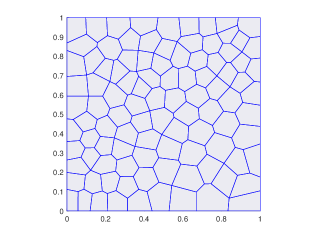
(a) $\{\mathcal{T}_{h}^{a}\}_{100}$

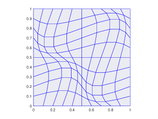
(b) $\{\mathcal{T}_{h}^{b}\}_{100}$

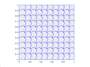
(c) $\{\mathcal{T}_{h}^{c}\}_{100}$

Figure 1: A set of coarse polygonal meshes ($N_{t}^{i}=100$) used to the first numerical experiment.

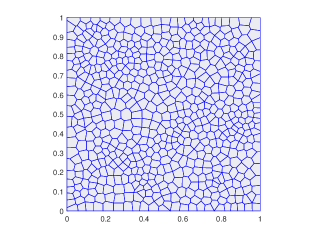
(a) $\{\mathcal{T}_{h}^{a}\}_{625}$

(b) $\{\mathcal{T}_{h}^{b}\}_{625}$

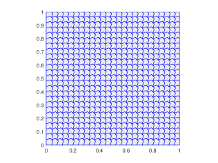
(c) $\{\mathcal{T}_{h}^{c}\}_{625}$

Figure 2: A set of fine polygonal meshes ($N_{t}^{i}=625$) used to the first numerical experiment.

In order to continue the convergence test, we have to note that the VEM solutions $\boldsymbol{u}_{h}$ and $\boldsymbol{J}_{h}$ are not explicitly known inside the elements, so we choose polynomial projections $\mathrm{\Pi}_{k_{1}}^{\nabla}\boldsymbol{u}$ and $\mathrm{\Pi}_{k_{2}}^{0}\boldsymbol{J}$ to compare with $\boldsymbol{u}$ and $\boldsymbol{J}$, respectively. Additionally, the variables $p_{h}$ and $\phi_{h}$ are piecewise polynomials such that we can directly to compute errors. In short, we apply the computable scheme

$$\text{error}(\boldsymbol{u},H^{1}):=\sqrt{\sum_{E\in\mathcal{T}_{h}}\|\nabla\boldsymbol{u}-\nabla\mathrm{\Pi}_{k_{1}}^{\nabla}\boldsymbol{u}\|_{0,E}^{2}},$$

$$\text{error}(\boldsymbol{J},L^{2}):=\sqrt{\sum_{E\in\mathcal{T}_{h}}\|\boldsymbol{J}-\mathrm{\Pi}_{k_{2}}^{0}\boldsymbol{J}\|_{0,E}^{2}},$$

$$\text{error}(p,L^{2}):=\|p-p_{h}\|_{0,\mathrm{\Omega}},\quad\text{error}(\phi,L^{2}):=\|\phi-\phi_{h}\|_{0,\mathrm{\Omega}},$$

and we associate with each discretization an average mehs-size

$$h:=\frac{1}{N_{t}}\sum_{j=1}^{N_{t}}h_{E_{j}}.$$

Next, we give the convergent order test under the first set of polynomial degree of accuracy $k_{1}=2$, $k_{2}=1$, and we consider three different types of meshes, see Fig.3-4. It is not difficult see that the convergence rates in Fig.3-4 achieve the expected results.

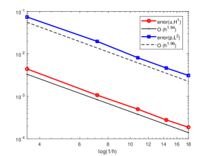
(a) $\{\mathcal{T}_{h}^{a}\}_{N_{t}^{a}}$

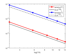
(b) $\{\mathcal{T}_{h}^{b}\}_{N_{t}^{b}}$

(c) $\{\mathcal{T}_{h}^{c}\}_{N_{t}^{c}}$

Figure 3: Convergence lines for the velocity and pressure with $k_{1}=2$, $k_{2}=1$.

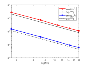
(a) $\{\mathcal{T}_{h}^{a}\}_{N_{t}^{a}}$

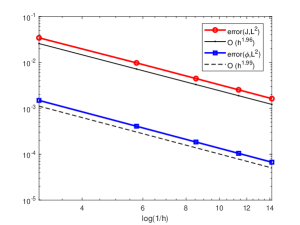
(b) $\{\mathcal{T}_{h}^{b}\}_{N_{t}^{b}}$

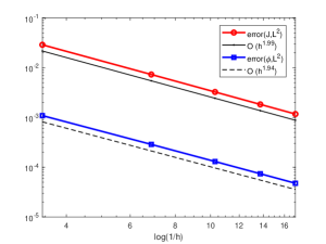
(c) $\{\mathcal{T}_{h}^{c}\}_{N_{t}^{c}}$

Figure 4: Convergence lines for the current density and electric potential with $k_{1}=2$, $k_{2}=1$.

Moreover, we also give the convergent order test under the first set of polynomial degree of accuracy $k_{1}=3$, $k_{2}=2$, and we consider three different types of meshes, see Fig.1-2. It is not difficult see that the convergence rates in Fig.5-6 achieve the expected results.

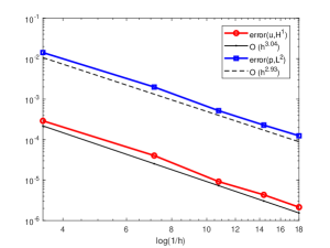
(a) $\{\mathcal{T}_{h}^{a}\}_{N_{t}^{a}}$

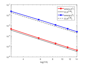
(b) $\{\mathcal{T}_{h}^{b}\}_{N_{t}^{b}}$

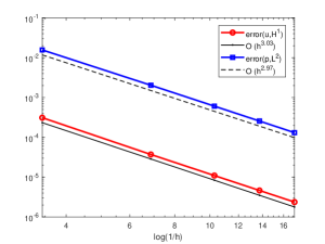
(c) $\{\mathcal{T}_{h}^{c}\}_{N_{t}^{c}}$

Figure 5: Convergence lines for the velocity and pressure with $k_{1}=3$, $k_{2}=2$.

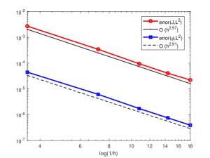
(a) $\{\mathcal{T}_{h}^{a}\}_{N_{t}^{a}}$

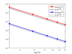
(b) $\{\mathcal{T}_{h}^{b}\}_{N_{t}^{b}}$

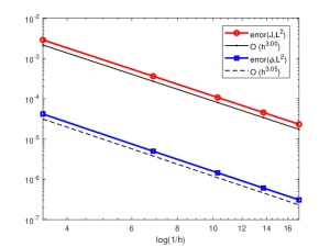
(c) $\{\mathcal{T}_{h}^{c}\}_{N_{t}^{c}}$

Figure 6: Convergence lines for the current density and electric potential with $k_{1}=3$, $k_{2}=2$.

Finally, we give the results of conservation properties through Table 1. We find that the proposed method fully satisfies the conservations of mass and charge, that is, both $\nabla\cdot\boldsymbol{u}_{h}=0$ and $\nabla\cdot\boldsymbol{J}_{h}=0$ achieve machine accuracy.

Table 1: Conservation of the proposed method under three types of meshes

		$k_{1}=2$		$k_{2}=1$
$\quad\{\mathcal{T}_{h}^{a}\}_{N_{t}^{a}}$	$N_{t}^{a}$	25	100	225	400	625
	$\|\nabla\cdot\boldsymbol{u}_{h}\|_{0}$	8.5688e-07	2.8491e-07	6.6119e-09	2.4267e-08	8.7604e-10
	$\|\nabla\cdot\boldsymbol{J}_{h}\|_{0}$	2.7686e-15	5.7942e-15	8.7247e-15	1.1518e-14	1.4877e-14
$\quad\{\mathcal{T}_{h}^{b}\}_{N_{t}^{b}}$	$N_{t}^{b}$	25	100	225	400	625
	$\|\nabla\cdot\boldsymbol{u}_{h}\|_{0}$	1.5832e-16	2.7300e-16	4.8885e-16	6.5470e-16	8.7174e-16
	$\|\nabla\cdot\boldsymbol{J}_{h}\|_{0}$	3.0312e-15	5.9777e-15	9.5903e-15	1.3096e-14	1.6391e-14
$\quad\{\mathcal{T}_{h}^{c}\}_{N_{t}^{c}}$	$N_{t}^{c}$	25	100	225	400	625
	$\|\nabla\cdot\boldsymbol{u}_{h}\|_{0}$	1.1745e-16	2.6489e-16	3.9901e-16	4.8691e-16	6.2374e-16
	$\|\nabla\cdot\boldsymbol{J}_{h}\|_{0}$	2.9465e-15	6.0252e-15	9.4660e-15	1.2578e-14	1.5259e-14
		$k_{1}=3$		$k_{2}=2$
$\quad\{\mathcal{T}_{h}^{a}\}_{N_{t}^{a}}$	$N_{t}^{a}$	25	100	225	400	625
	$\|\nabla\cdot\boldsymbol{u}_{h}\|_{0}$	8.2948e-10	6.8605e-11	4.3703e-13	1.6281e-12	2.6458e-14
	$\|\nabla\cdot\boldsymbol{J}_{h}\|_{0}$	3.8793e-15	8.4146e-15	1.3391e-14	1.7778e-14	2.2439e-14
$\quad\{\mathcal{T}_{h}^{b}\}_{N_{t}^{b}}$	$N_{t}^{b}$	25	100	225	400	625
	$\|\nabla\cdot\boldsymbol{u}_{h}\|_{0}$	6.7811e-16	1.1385e-15	2.1360e-15	2.9119e-15	3.7930e-15
	$\|\nabla\cdot\boldsymbol{J}_{h}\|_{0}$	5.2034e-15	1.0417e-14	1.7125e-14	2.2661e-14	2.7996e-14
$\quad\{\mathcal{T}_{h}^{c}\}_{N_{t}^{c}}$	$N_{t}^{c}$	25	100	225	400	625
	$\|\nabla\cdot\boldsymbol{u}_{h}\|_{0}$	3.8742e-16	5.8802e-16	8.5715e-16	1.0343e-15	1.3430e-15
	$\|\nabla\cdot\boldsymbol{J}_{h}\|_{0}$	4.8106e-15	9.4772e-15	1.3886e-14	1.7857e-14	2.2509e-14

5.2 Robustness of pressure and electric potential- Revise by using Newton iterative

In this subsection, the robustness of the pressure and the electric potential are only investigated under the situation $k_{1}=2$ and $k_{2}=1$. In other higher-order cases, we can still obtain similar results. Referencing john2017divergence ; zhang2021coupled ; zhang2022fully , we set $\mathrm{\Omega}=[0,1]^{2}$, $\boldsymbol{B}=(0,0,1)$, $\nu=Sc=1$, and choose the force terms $\boldsymbol{f}$ and $\boldsymbol{g}$ such that the exact solutions are given by

$$\boldsymbol{u}=(0,0),\quad p=(x^{3}+2x^{2}-\frac{11}{12})s_{1},$$

$$\boldsymbol{J}=(0,0),\quad\phi=(x^{2}+x-\frac{5}{6})s_{2},$$

where $s_{1},s_{2}\leq 0$ are parameters.

On the one hand, we set $s_{1}=0$ and vary $s_{2}$ from 1, 100, 10000. According to the errors of the numerical solutions given in Tables 2-4, we observe that the errors in velocity, pressure, and current density are independent of the mesh at a fixed $s_{2}$. As varying $s_{2}$ from 1, 100, 10000, due to an increase in the right-hand side function $\boldsymbol{g}$ such that the errors of numerical solutions will have a little bigger. In addition, the errors for electric potential converge optimally. The results show that our scheme is robust with respect to the electric potential.

Table 2: Robustness of the electric potential with $s_{2}=1,100,10000$ under three types of meshes.

$s_{2}=1$		$k_{1}=2$		$k_{2}=1$
$\quad\{\mathcal{T}_{h}^{a}\}_{N_{t}^{a}}$	$N_{t}^{a}$	25	100	225	400	625
	$\|\boldsymbol{u}-\boldsymbol{u}_{h}\|_{1}$	1.4038e-17	2.2981e-17	3.0505e-17	3.9662e-17	4.5267e-17
	$\|p-p_{h}\|_{0}$	5.5188e-17	3.6679e-17	4.9080e-17	3.7742e-17	4.2697e-17
	$\|\boldsymbol{J}-\boldsymbol{J}_{h}\|_{0}$	1.1694e-15	2.3260e-15	3.5396e-15	5.0605e-15	6.9883e-15
	$\|\phi-\phi_{h}\|_{0}$	3.7525e-03(-)	1.0049e-03(1.84)	4.1406e-04(2.05)	2.3643e-04(1.91)	1.4899e-04(2.09)
$\quad\{\mathcal{T}_{h}^{b}\}_{N_{t}^{b}}$	$N_{t}^{b}$	25	100	225	400	625
	$\|\boldsymbol{u}-\boldsymbol{u}_{h}\|_{1}$	1.0300e-17	1.3279e-17	1.3266e-17	1.6146e-17	1.6368e-17
	$\|p-p_{h}\|_{0}$	6.8436e-17	5.6800e-17	3.9894e-17	3.6314e-17	3.5646e-17
	$\|\boldsymbol{J}-\boldsymbol{J}_{h}\|_{0}$	1.2599e-15	2.2999e-15	3.5039e-15	4.2394e-15	5.6181e-15
	$\|\phi-\phi_{h}\|_{0}$	4.2123e-03(-)	1.1670e-03(1.97)	5.2978e-04(1.99)	3.0027e-04(1.99)	1.9285e-04(2.00)
$\quad\{\mathcal{T}_{h}^{c}\}_{N_{t}^{c}}$	$N_{t}^{c}$	25	100	225	400	625
	$\|\boldsymbol{u}-\boldsymbol{u}_{h}\|_{1}$	2.1006e-17	2.9916e-17	3.7833e-17	4.6568e-17	5.0823e-17
	$\|p-p_{h}\|_{0}$	7.6793e-17	6.3892e-17	4.5267e-17	4.9397e-17	4.9483e-17
	$\|\boldsymbol{J}-\boldsymbol{J}_{h}\|_{0}$	1.3120e-15	3.0357e-15	4.4069e-15	6.1490e-15	7.2545e-15
	$\|\phi-\phi_{h}\|_{0}$	3.3705e-03(-)	8.3988e-04(2.00)	3.7286e-04(2.00)	2.0961e-04(2.00)	1.3411e-04(2.00)
$s_{2}=100$		$k_{1}=2$		$k_{2}=1$
$\quad\{\mathcal{T}_{h}^{a}\}_{N_{t}^{a}}$	$N_{t}^{a}$	25	100	225	400	625
	$\|\boldsymbol{u}-\boldsymbol{u}_{h}\|_{1}$	1.2840e-15	2.4069e-15	3.1347e-15	4.0484e-15	5.0694e-15
	$\|p-p_{h}\|_{0}$	7.1870e-15	3.9017e-15	4.4053e-15	3.8523e-15	3.9589e-15
	$\|\boldsymbol{J}-\boldsymbol{J}_{h}\|_{0}$	1.1714e-13	2.3217e-13	3.6027e-13	5.0793e-13	7.3304e-13
	$\|\phi-\phi_{h}\|_{0}$	3.7525e-01(-)	1.0049e-01(1.85)	4.1406e-02(2.05)	2.3643e-02(1.91)	1.4899e-02(2.09)
$\quad\{\mathcal{T}_{h}^{b}\}_{N_{t}^{b}}$	$N_{t}^{b}$	25	100	225	400	625
	$\|\boldsymbol{u}-\boldsymbol{u}_{h}\|_{1}$	9.4523e-16	1.4999e-15	1.2935e-15	1.6928e-15	1.6773e-15
	$\|p-p_{h}\|_{0}$	7.0120e-15	4.1375e-15	3.7761e-15	3.5601e-15	4.2104e-15
	$\|\boldsymbol{J}-\boldsymbol{J}_{h}\|_{0}$	1.2035e-13	2.3500e-13	3.4596e-13	4.1909e-13	5.4691e-13
	$\|\phi-\phi_{h}\|_{0}$	4.2123e-01(-)	1.1670e-01(1.97)	5.2978e-02(1.99)	3.0027e-02(1.99)	1.9285e-02(2.00)
$\quad\{\mathcal{T}_{h}^{c}\}_{N_{t}^{c}}$	$N_{t}^{c}$	25	100	225	400	625
	$\|\boldsymbol{u}-\boldsymbol{u}_{h}\|_{1}$	2.4746e-15	2.6882e-15	3.7472e-15	4.4290e-15	6.0902e-15
	$\|p-p_{h}\|_{0}$	7.6446e-15	6.3170e-15	4.3570e-15	5.0499e-15	4.4499e-15
	$\|\boldsymbol{J}-\boldsymbol{J}_{h}\|_{0}$	1.5589e-13	3.0238e-13	4.4964e-13	6.2002e-13	7.4859e-13
	$\|\phi-\phi_{h}\|_{0}$	3.3705e-01(-)	8.3988e-02(2.00)	3.7286e-02(2.00)	2.0961e-02(2.00)	1.3411e-02(2.00)
$s_{2}=10000$		$k_{1}=2$		$k_{2}=1$
$\quad\{\mathcal{T}_{h}^{a}\}_{N_{t}^{a}}$	$N_{t}^{a}$	25	100	225	400	625
	$\|\boldsymbol{u}-\boldsymbol{u}_{h}\|_{1}$	1.4234e-13	2.0567e-13	3.0912e-13	3.9268e-13	4.6491e-13
	$\|p-p_{h}\|_{0}$	6.8886e-13	4.3126e-13	4.1756e-13	3.6822e-13	3.8735e-13
	$\|\boldsymbol{J}-\boldsymbol{J}_{h}\|_{0}$	1.1725e-11	2.3065e-11	3.5231e-11	5.0388e-11	7.0641e-11
	$\|\phi-\phi_{h}\|_{0}$	3.7525e+01(-)	1.0049e+01(1.85)	4.1406e+00(2.05)	2.3643e+00(1.91)	1.4899e+00(2.09)
$\quad\{\mathcal{T}_{h}^{b}\}_{N_{t}^{b}}$	$N_{t}^{b}$	25	100	225	400	625
	$\|\boldsymbol{u}-\boldsymbol{u}_{h}\|_{1}$	8.6213e-14	1.2054e-13	1.3848e-13	1.4475e-13	1.8435e-13
	$\|p-p_{h}\|_{0}$	6.0537e-13	4.5795e-13	3.9193e-13	3.3546e-13	4.1438e-13
	$\|\boldsymbol{J}-\boldsymbol{J}_{h}\|_{0}$	1.1377e-11	2.2713e-11	3.5203e-11	4.0336e-11	5.7377e-11
	$\|\phi-\phi_{h}\|_{0}$	4.2123e+01(-)	1.1670e+01(1.97)	5.2978e+00(1.99)	3.0027e+00(1.99)	1.9285e+00(2.00)
$\quad\{\mathcal{T}_{h}^{c}\}_{N_{t}^{c}}$	$N_{t}^{c}$	25	100	225	400	625
	$\|\boldsymbol{u}-\boldsymbol{u}_{h}\|_{1}$	2.5246e-13	2.5583e-13	3.6619e-13	4.9866e-13	5.6965e-13
	$\|p-p_{h}\|_{0}$	8.8202e-13	6.4251e-13	5.6004e-13	5.3525e-13	5.3539e-13
	$\|\boldsymbol{J}-\boldsymbol{J}_{h}\|_{0}$	1.5581e-11	2.9220e-11	4.3027e-11	6.1705e-11	7.1356e-11
	$\|\phi-\phi_{h}\|_{0}$	3.3705e+01(-)	8.3988e+00(2.01)	3.7286e+00(2.00)	2.0961e+00(2.00)	1.3411e+00(2.00)

On the other hand, we set $s_{2}=0$ and vary $s_{1}$ from 1, 100, 10000. According to the errors of the numerical solutions given in Tables 5-7, we observe that the errors in velocity, pressure, and current density are independent of the mesh at a fixed $s_{1}$. As varying $s_{1}$ from 1, 100, 10000, due to an increase in the right-hand side function $\boldsymbol{f}$ such that the errors of numerical solutions will have a little bigger. In addition, the errors for electric potential converge optimally. The results show that our scheme is robust with respect to the electric potential.

Table 3: Robustness of the pressure with $s_{1}=1,\;100,\;10000$ under three types of meshes.

$s_{1}=1$		$k_{1}=2$		$k_{2}=1$
$\quad\{\mathcal{T}_{h}^{a}\}_{N_{t}^{a}}$	$N_{t}^{a}$	25	100	225	400	625
	$\|\boldsymbol{u}-\boldsymbol{u}_{h}\|_{1}$	1.1586e-16	8.9756e-17	8.6007e-17	8.8406e-17	8.3868e-17
	$\|p-p_{h}\|_{0}$	1.3033e-02(-)	3.5604e-03(1.82)	1.4612e-03(2.06)	8.6327e-04(1.79)	5.5409e-04(2.01)
	$\|\boldsymbol{J}-\boldsymbol{J}_{h}\|_{0}$	2.2776e-18	1.0237e-18	8.4768e-19	6.8322e-19	5.9517e-19
	$\|\phi-\phi_{h}\|_{0}$	7.0098e-19	6.3796e-19	3.2599e-19	2.8614e-19	3.1854e-19
$\quad\{\mathcal{T}_{h}^{b}\}_{N_{t}^{b}}$	$N_{t}^{b}$	25	100	225	400	625
	$\|\boldsymbol{u}-\boldsymbol{u}_{h}\|_{1}$	7.9077e-17	8.1391e-17	9.2824e-17	8.1362e-17	8.0287e-17
	$\|p-p_{h}\|_{0}$	1.5147e-02(-)	4.2029e-03(1.97)	1.9084e-03(1.99)	1.0818e-03(1.99)	6.9481e-04(2.00)
	$\|\boldsymbol{J}-\boldsymbol{J}_{h}\|_{0}$	9.9887e-19	8.6839e-19	8.7459e-19	6.3256e-19	5.3379e-19
	$\|\phi-\phi_{h}\|_{0}$	6.0627e-19	3.4229e-19	2.7354e-19	2.3673e-19	2.1563e-19
$\quad\{\mathcal{T}_{h}^{c}\}_{N_{t}^{c}}$	$N_{t}^{c}$	25	100	225	400	625
	$\|\boldsymbol{u}-\boldsymbol{u}_{h}\|_{1}$	1.2267e-16	1.0013e-16	9.3688e-17	9.9873e-17	7.9725e-17
	$\|p-p_{h}\|_{0}$	1.1462e-02(-)	2.9339e-03(1.97)	1.3157e-03(1.98)	7.4352e-04(1.98)	4.7721e-04(1.99)
	$\|\boldsymbol{J}-\boldsymbol{J}_{h}\|_{0}$	4.1419e-18	1.8081e-18	1.2560e-18	1.0301e-18	6.9548e-19
	$\|\phi-\phi_{h}\|_{0}$	7.7735e-19	3.4985e-19	3.5279e-19	2.8518e-19	1.7725e-19
$s_{1}=100$		$k_{1}=2$		$k_{2}=1$
$\quad\{\mathcal{T}_{h}^{a}\}_{N_{t}^{a}}$	$N_{t}^{a}$	25	100	225	400	625
	$\|\boldsymbol{u}-\boldsymbol{u}_{h}\|_{1}$	9.5984e-15	7.7415e-15	9.0305e-15	8.7799e-15	8.1488e-15
	$\|p-p_{h}\|_{0}$	1.3033e+00(-)	3.5604e-01(1.82)	1.4612e-01(2.06)	8.6327e-02(1.79)	5.5409e-02(2.01)
	$\|\boldsymbol{J}-\boldsymbol{J}_{h}\|_{0}$	1.8599e-16	9.5700e-17	8.8457e-17	6.8496e-17	5.9400e-17
	$\|\phi-\phi_{h}\|_{0}$	4.2950e-17	2.4435e-17	4.1856e-17	3.2372e-17	1.7283e-17
$\quad\{\mathcal{T}_{h}^{b}\}_{N_{t}^{b}}$	$N_{t}^{b}$	25	100	225	400	625
	$\|\boldsymbol{u}-\boldsymbol{u}_{h}\|_{1}$	7.8585e-15	8.9846e-15	8.9851e-15	8.3134e-15	7.8817e-15
	$\|p-p_{h}\|_{0}$	1.5147e+00(-)	4.2029e-01(1.97)	1.9084e-01(1.99)	1.0818e-01(1.99)	6.9481e-02(2.00)
	$\|\boldsymbol{J}-\boldsymbol{J}_{h}\|_{0}$	9.6668e-17	9.9319e-17	8.6918e-17	6.1416e-17	5.2059e-17
	$\|\phi-\phi_{h}\|_{0}$	2.9379e-17	2.1606e-17	2.1082e-17	2.8409e-17	1.6956e-17
$\quad\{\mathcal{T}_{h}^{c}\}_{N_{t}^{c}}$	$N_{t}^{c}$	25	100	225	400	625
	$\|\boldsymbol{u}-\boldsymbol{u}_{h}\|_{1}$	1.1457e-14	1.0516e-14	9.3583e-15	9.6834e-15	7.8838e-15
	$\|p-p_{h}\|_{0}$	1.1462e+00(-)	2.9339e-01(1.97)	1.3157e-01(1.98)	7.4352e-02(1.98)	4.7721e-02(1.99)
	$\|\boldsymbol{J}-\boldsymbol{J}_{h}\|_{0}$	3.6189e-16	1.9780e-16	1.2236e-16	1.0353e-16	6.8903e-17
	$\|\phi-\phi_{h}\|_{0}$	5.3327e-17	4.0973e-17	2.1874e-17	1.6691e-17	2.6032e-17
$s_{1}=10000$		$k_{1}=2$		$k_{2}=1$
$\quad\{\mathcal{T}_{h}^{a}\}_{N_{t}^{a}}$	$N_{t}^{a}$	25	100	225	400	625
	$\|\boldsymbol{u}-\boldsymbol{u}_{h}\|_{1}$	1.0344e-12	8.6090e-13	8.4833e-13	8.2517e-13	8.0170e-13
	$\|p-p_{h}\|_{0}$	1.3033e+02(-)	3.5604e+01(1.82)	1.4612e+01(2.06)	8.6327e+00(1.80)	5.5409e+00(2.01)
	$\|\boldsymbol{J}-\boldsymbol{J}_{h}\|_{0}$	2.2218e-14	1.0016e-14	8.4395e-15	6.7571e-15	5.8470e-15
	$\|\phi-\phi_{h}\|_{0}$	3.1215e-15	2.2643e-15	2.2568e-15	2.3685e-15	1.0430e-15
$\quad\{\mathcal{T}_{h}^{b}\}_{N_{t}^{b}}$	$N_{t}^{b}$	25	100	225	400	625
	$\|\boldsymbol{u}-\boldsymbol{u}_{h}\|_{1}$	1.0834e-12	9.0888e-13	9.3482e-13	8.2879e-13	7.8379e-13
	$\|p-p_{h}\|_{0}$	1.5147e+02(-)	4.2029e+01(1.97)	1.9084e+01(1.99)	1.0818e+01(1.99)	6.9481e+00(2.00)
	$\|\boldsymbol{J}-\boldsymbol{J}_{h}\|_{0}$	1.4619e-14	9.9619e-15	8.3761e-15	6.1658e-15	5.3620e-15
	$\|\phi-\phi_{h}\|_{0}$	1.0911e-14	3.4001e-15	3.8574e-15	3.0887e-15	1.4449e-15
$\quad\{\mathcal{T}_{h}^{c}\}_{N_{t}^{c}}$	$N_{t}^{c}$	25	100	225	400	625
	$\|\boldsymbol{u}-\boldsymbol{u}_{h}\|_{1}$	1.2496e-12	1.0182e-12	9.2227e-13	9.8056e-13	7.6705e-13
	$\|p-p_{h}\|_{0}$	1.1462e+02(-)	2.9339e+01(1.97)	1.3157e+01(1.98)	7.4352e+00(1.98)	4.7721e+00(1.99)
	$\|\boldsymbol{J}-\boldsymbol{J}_{h}\|_{0}$	3.6673e-14	1.9954e-14	1.2263e-14	1.0301e-14	6.8154e-15
	$\|\phi-\phi_{h}\|_{0}$	8.2712e-15	4.4074e-15	2.5894e-15	1.5982e-15	1.7892e-15

Overall, the robustness of the pressure and the electric potential are satisfied under our scheme and the results are consistent with the predictions in Theorem 22.

5.3 Inductionless MHD problem with singular solution

In this subsection, the inductionless MHD problem with singular solution is considered in a non-convex L-shaped domain $\mathrm{\Omega}=[-0.5,0.5]\times[-0.5,0.5]\setminus[0,0.5]\times(-0.5,0]$ to verify the ability of the proposed method to capture the singularities. Let $\boldsymbol{B}=(0,0,1)$, $Re=Sc=1$, and the functions $\boldsymbol{f}$ and $\boldsymbol{g}$ such that exact solution is

$$u_{1}(r,\vartheta)=r^{\varepsilon}\big{(}(1+\varepsilon)\sin(\vartheta)\Theta(\vartheta)+\cos(\vartheta)\Theta^{{}^{\prime}}(\vartheta)\big{)},\quad u_{2}=r^{\varepsilon}\big{(}-(1+\varepsilon)\cos(\vartheta)\Theta(\vartheta)+\sin(\vartheta)\Theta^{{}^{\prime}}(\vartheta)\big{)},$$

$$p(r,\vartheta)=-r^{\varepsilon-1}\big{(}(1+\varepsilon)^{2}\Theta^{{}^{\prime}}(\vartheta)+\Theta^{{}^{\prime\prime\prime}}(\vartheta)\big{)}/(1-\varepsilon),\quad\phi(r,\vartheta)=0,$$

$$J_{1}(r,\vartheta)=-\big{(}2\sin(\vartheta/3)\big{)}/(3r^{1/3}),\quad J_{2}(r,\vartheta)=\big{(}2\cos(\vartheta/3)\big{)}/(3r^{1/3}),$$

where $(r,\vartheta)$ denotes the polar coordinate, $\mu=\frac{3\pi}{2}$, the value of the parameter $\varepsilon$ is the smallest positive solution of $\sin(\varepsilon\mu)+\varepsilon\sin(\mu)=0$ and

$$\Theta(\vartheta)=\sin\big{(}(1+\varepsilon)\vartheta\big{)}\cos(\varepsilon\mu)/(1+\varepsilon)-\cos\big{(}(1+\varepsilon)-\sin\big{(}(1-\varepsilon)\vartheta\big{)}\cos(\varepsilon\mu)/(1-\varepsilon)+\cos\big{(}(1-\varepsilon).$$

Significantly, we get $(\boldsymbol{u},p)\in\boldsymbol{H}^{1+\varepsilon}\times H^{\varepsilon}$ and $\boldsymbol{J}\in\boldsymbol{H}^{2/3}$. the conductive boundary condition is considered in this example, it means that the electric potential $\phi=0$ on $\partial\mathrm{\Omega}$. By observing, we can clearly determine that the exact solution have strong singularity at the corner.

Due to the low regularity of the exact solutions, the pursuit of using higher-order schemes to solve this problem may slightly reduce the error but will not change the convergence law. Therefore, we only provide the calculation results under situation $k_{1}=2$ and $k_{2}=1$ here. From the errors and convergence rates of the numerical solutions under the L-domain triangular meshes $\{\mathcal{T}_{h}^{L}\}_{N_{t}^{L}}$ given in Table 4, we can conclude that the convergence rates are consistent with the results of Theorem 22 in theoretical analysis. Moreover, the discrete velocity and current density also satisfy the conditions of divergence-fee. Finally, we display the numerical solution on the grid $\{\mathcal{T}_{h}^{L}\}_{384}$ in figure 7, which clearly shows that the proposed method can effectively capture singularities.

Table 4: The errors and convergence rates of numerical solutions under triangular meshes—Revise-data $\{\mathcal{T}_{h}^{L}\}_{N_{t}^{L}}$.

$N_{t}^{L}$	$\|\boldsymbol{u}-\boldsymbol{u}_{h}\|_{1}$	$\|p-p_{h}\|_{0}$	$\|\boldsymbol{J}-\boldsymbol{J}_{h}\|_{0}$	$\|\phi-\phi_{h}\|_{0}$	$\|\nabla\cdot\boldsymbol{u}_{h}\|_{0}$	$\|\nabla\cdot\boldsymbol{J}_{h}\|_{0}\quad$
96	5.1869e-01(-)	6.7796e-01(-)	4.3097e-02(-)	9.3642e-04(-)	3.2502e-11	8.9327e-15
384	3.5333e-01(0.554)	4.3717e-01(0.633)	2.7374e-02(0.655)	3.8768e-04(1.272)	1.1154e-11	1.7795e-14
1536	2.4159e-01(0.548)	2.9173e-01(0.584)	1.7308e-02(0.661)	1.7780e-04(1.124)	3.8246e-12	3.5711e-14
1944	2.2651e-01(0.547)	2.7281e-01(0.569)	1.6007e-02(0.663)	1.5661e-04(1.077)	3.1884e-12	4.0106e-14
2345	1.9356e-01(0.546)	2.3191e-01(0.565)	1.3223e-02(0.664)	1.1532e-04(1.063)	2.0447e-12	5.3722e-14

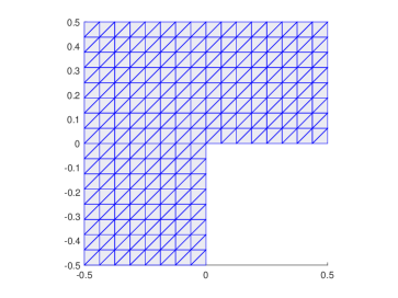
(a) $\{\mathcal{T}_{h}^{L}\}_{384}$

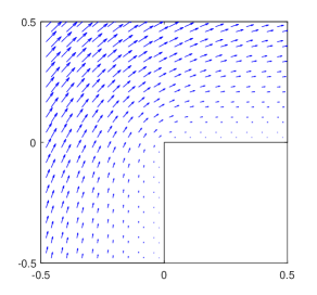
(b) Numerical approximation of $\boldsymbol{u}$

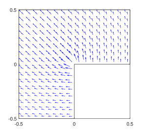
(c) Numerical approximation of $\boldsymbol{J}$

Figure 7: A set of fine polygonal meshes ($N_{t}^{i}=625$) used to the first numerical experiment.

5.4 The inductionless MHD flow around a circular cylinder

In this subsection, we consider a type of 2D benchmark problem, which is the flow around a circular cylinder liu2022pressure . The main feature of this model is that with the change of Reynolds number from low to high, the flow of the fluid will gradually evolve into a flow that loses symmetry, rather than maintaining non-separation from the cylinder, without vortices, and the upstream and downstream flow lines of the cylinder are symmetrical. The physical structure, boundary conditions and mesh used for this numerical simulation see Fig.8.

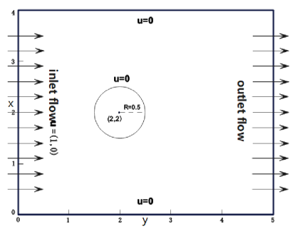
(a) Physical structure

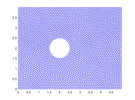
(b) $\{\mathcal{T}_{h}^{c}\}_{3000}$

Figure 8: Physical structure and mesh used for the numerical simulation.

Obviously, we can clearly observing that the streamlines of cylinder are symmetric about both $x=2$ and $y=2$ at $\nu=1$ and the fluid flowing near the top of the cylinder begins to separate and forms a fixed pair of symmetrical eddies downstream of the cylinder at $\nu=0.01$. This is consistent with the theoretical analysis of physical phenomena.

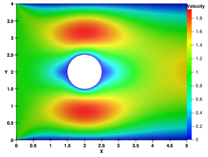
(a) Counter

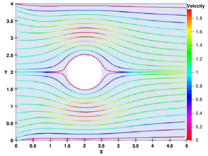
(b) Streamlines

Figure 9: Counter and streamlines of discrete velocity $\boldsymbol{u}_{h}$ at $\nu=1$.

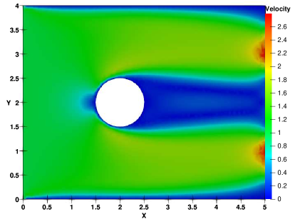
(a) Counter

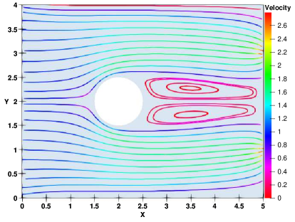
(b) Streamlines

Figure 10: Counter and streamlines of discrete velocity $\boldsymbol{u}_{h}$ at $\nu=0.01$.

5.5 The backstage step inductionless MHD flow

6 Conclusion

In this paper, we present a full divergence-free of high order virtual finite element method to approximation of stationary inductionless magnetohydrodynamic equations on polygonal meshes and process rigorous error analysis to show that the proposed method is stable and convergent. In the following work, we will propose the lowest order 2D/3D virtual finite element method to solve the steady inductionless MHD equations. Of course, this format still satisfies full divergence-free.

References

- [1] Robert A Adams and John JF Fournier. Sobolev spaces. Elsevier, 2003.
- [2] Bashir Ahmad, Ahmed Alsaedi, Franco Brezzi, L Donatella Marini, and Alessandro Russo. Equivalent projectors for virtual element methods. Computers & Mathematics with Applications, 66(3):376–391, 2013.
- [3] L Beirão da Veiga, F Brezzi, LD Marini, and A Russo. H(div) and H-conforming vem. arXiv e-prints, pages arXiv–1407, 2014.
- [4] L Beirão da Veiga, Franco Brezzi, Andrea Cangiani, Gianmarco Manzini, L Donatella Marini, and Alessandro Russo. Basic principles of virtual element methods. Mathematical Models and Methods in Applied Sciences, 23(01):199–214, 2013.
- [5] L Beirão da Veiga, Franco Brezzi, Luisa Donatella Marini, and Alessandro Russo. The hitchhiker’s guide to the virtual element method. Mathematical models and methods in applied sciences, 24(08):1541–1573, 2014.
- [6] L Beirão da Veiga, Franco Dassi, and Giuseppe Vacca. The stokes complex for virtual elements in three dimensions. Mathematical Models and Methods in Applied Sciences, 30(03):477–512, 2020.
- [7] L Beirão da Veiga, David Mora, and Giuseppe Vacca. The stokes complex for virtual elements with application to navier–stokes flows. Journal of Scientific Computing, 81:990–1018, 2019.
- [8] Lourenço Beirão da Veiga, Franco Brezzi, Luisa Donatella Marini, and Alessandro Russo. Mixed virtual element methods for general second order elliptic problems on polygonal meshes. ESAIM: Mathematical Modelling and Numerical Analysis-Modélisation Mathématique et Analyse Numérique, 50(3):727–747, 2016.
- [9] Lourenço Beirão da Veiga, Franco Dassi, Gianmarci Manzini, and Lorenzo Mascotto. The virtual element method for the 3D resistive magnetohydrodynamic model. Mathematical Models and Methods in Applied Sciences, 33(03):643–686, 2023.
- [10] S. C. Brenner and L. Y. Sung. Virtual Element Methods on Meshes with Small Edges or Faces. Mathematical Models Methods in Applied Sciences, 2017.
- [11] Susanne C Brenner. The mathematical theory of finite element methods. Springer, 2008.
- [12] Franco Brezzi, Richard S Falk, and L Donatella Marini. Basic principles of mixed virtual element methods. ESAIM: Mathematical Modelling and Numerical Analysis, 48(4):1227–1240, 2014.
- [13] Ernesto Cáceres, Gabriel N Gatica, and Filánder A Sequeira. A mixed virtual element method for the Brinkman problem. Mathematical Models and Methods in Applied Sciences, 27(04):707–743, 2017.
- [14] Long Chen and Feng Wang. A divergence free weak virtual element method for the stokes problem on polytopal meshes. Journal of Scientific Computing, 78:864–886, 2019.
- [15] L Beirão da Veiga, Franco Brezzi, Franco Dassi, L Donatella Marini, and Alessandro Russo. A family of three-dimensional virtual elements with applications to magnetostatics. SIAM Journal on Numerical Analysis, 56(5):2940–2962, 2018.
- [16] L Beirão da Veiga, Franco Dassi, Gianmarco Manzini, and Lorenzo Mascotto. Virtual elements for maxwell’s equations. Computers & Mathematics with Applications, 116:82–99, 2022.
- [17] L Beirão Da Veiga, Carlo Lovadina, and Giuseppe Vacca. Virtual elements for the Navier-Stokes problem on polygonal meshes. SIAM Journal on Numerical Analysis, 56(3):1210–1242, 2018.
- [18] Lourenco Beirão da Veiga, Carlo Lovadina, and Giuseppe Vacca. Divergence free virtual elements for the Stokes problem on polygonal meshes. ESAIM: Mathematical Modelling and Numerical Analysis, 51(2):509–535, 2017.
- [19] Franco Dassi and Giuseppe Vacca. Bricks for the mixed high-order virtual element method: projectors and differential operators. Applied Numerical Mathematics, 155:140–159, 2020.
- [20] Shitian Dong, Xiaodi Zhang, and Haiyan Su. Electric potential-robust iterative analysis of charge-conservative conforming fem for thermally coupled inductionless mhd system. Communications in Nonlinear Science and Numerical Simulation, 120:107182, 2023.
- [21] Derk Frerichs and Christian Merdon. Divergence-preserving reconstructions on polygons and a really pressure-robust virtual element method for the stokes problem. IMA Journal of Numerical Analysis, 42(1):597–619, 2022.
- [22] Gabriel N Gatica, Mauricio Munar, and Filánder A Sequeira. A mixed virtual element method for the navier–stokes equations. Mathematical Models and Methods in Applied Sciences, 28(14):2719–2762, 2018.
- [23] Roland Glowinski and Olivier Pironneau. Finite element methods for navier-stokes equations. Annual review of fluid mechanics, 24(1):167–204, 1992.
- [24] Chen Greif, Dan Li, Dominik Schötzau, and Xiaoxi Wei. A mixed finite element method with exactly divergence-free velocities for incompressible magnetohydrodynamics. Computer Methods in Applied Mechanics and Engineering, 199(45-48):2840–2855, 2010.
- [25] César Herrera, Ricardo Corrales-Barquero, Jorge Arroyo-Esquivel, and Juan G Calvo. A numerical implementation for the high-order 2d virtual element method in matlab. Numerical Algorithms, 92(3):1707–1721, 2023.
- [26] Volker John, Alexander Linke, Christian Merdon, Michael Neilan, and Leo G Rebholz. On the divergence constraint in mixed finite element methods for incompressible flows. SIAM review, 59(3):492–544, 2017.
- [27] Lingxiao Li, Mingjiu Ni, and Weiying Zheng. A charge-conservative finite element method for inductionless mhd equations. part i: Convergence. SIAM Journal on Scientific Computing, (4), 2019.
- [28] Lingxiao Li, Mingjiu Ni, and Weiying Zheng. A charge-conservative finite element method for inductionless mhd equations. part ii: a robust solver. SIAM Journal on Scientific Computing, 41(4):B816–B842, 2019.
- [29] Xin Liu and Yufeng Nie. Pressure-independent velocity error estimates for (navier-) stokes nonconforming virtual element discretization with divergence free. Numerical Algorithms, 90(2):477–506, 2022.
- [30] Xiaonian Long. The analysis of finite element method for the inductionless MHD equations. PhD thesis, PhD Dissertation, University of Chinese Academy of Sciences, 2019.
- [31] Xiaonian Long and Qianqian Ding. Convergence analysis of a conservative finite element scheme for the thermally coupled incompressible inductionless mhd problem. Applied Numerical Mathematics, 182:176–195, 2022.
- [32] Xiaonian Long, Qianqian Ding, and Shipeng Mao. Error analysis of a conservative finite element scheme for time-dependent inductionless mhd problem. Journal of Computational and Applied Mathematics, 419:114728, 2023.
- [33] Gianmarco Manzini and Annamaria Mazzia. Conforming virtual element approximations of the two-dimensional stokes problem. Applied Numerical Mathematics, 181:176–203, 2022.
- [34] Ming-Jiu Ni and Jun-Feng Li. A consistent and conservative scheme for incompressible MHD flows at a low magnetic reynolds number. part iii: On a staggered mesh. Journal of Computational Physics, 231(2):281–298, 2012.
- [35] Ming-Jiu Ni, Ramakanth Munipalli, Peter Huang, Neil B Morley, and Mohamed A Abdou. A current density conservative scheme for incompressible mhd flows at a low magnetic reynolds number. part ii: On an arbitrary collocated mesh. Journal of Computational Physics, 227(1):205–228, 2007.
- [36] Ming-Jiu Ni, Ramakanth Munipalli, Neil B Morley, Peter Huang, and Mohamed A Abdou. A current density conservative scheme for incompressible mhd flows at a low magnetic reynolds number. part i: On a rectangular collocated grid system. Journal of Computational Physics, 227(1):174–204, 2007.
- [37] Ramon Planas, Santiago Badia, and Ramon Codina. Approximation of the inductionless MHD problem using a stabilized finite element method. Journal of Computational Physics, 230(8):2977–2996, 2011.
- [38] Giuseppe Vacca. An -conforming virtual element for Darcy and Brinkman equations. Mathematical Models and Methods in Applied Sciences, 28(01):159–194, 2018.
- [39] Xiaorong Wang and Xiaodi Zhang. Decoupled, linear, unconditionally energy stable and charge-conservative finite element method for an inductionless magnetohydrodynamic phase-field model. Mathematics and Computers in Simulation, 2023.
- [40] Xiaodi Zhang and Qianqian Ding. Coupled iterative analysis for stationary inductionless magnetohydrodynamic system based on charge-conservative finite element method. Journal of Scientific Computing, 88:1–32, 2021.
- [41] Xiaodi Zhang and Qianqian Ding. A decoupled, unconditionally energy stable and charge-conservative finite element method for inductionless magnetohydrodynamic equations. Computers & Mathematics with Applications, 127:80–96, 2022.
- [42] Xiaodi Zhang and Xiaorong Wang. A fully divergence-free finite element scheme for stationary inductionless magnetohydrodynamic equations. Journal of Scientific Computing, 90(2):70, 2022.
- [43] Xianghai Zhou, Haiyan Su, and Bo Tang. Two-level picard coupling correction finite element method based on charge-conservation for stationary inductionless magnetohydrodynamic equations. Computers & Mathematics with Applications, 115:41–56, 2022.