Decentralized Gradient-Free Methods for Stochastic Non-Smooth Non-Convex Optimization

Abstract

We consider decentralized gradient-free optimization of minimizing Lipschitz continuous functions that satisfy neither smoothness nor convexity assumption. We propose two novel gradient-free algorithms, the Decentralized Gradient-Free Method (DGFM) and its variant, the Decentralized Gradient-Free Method⁺ (DGFM⁺). Based on the techniques of randomized smoothing and gradient tracking, DGFM requires the computation of the zeroth-order oracle of a single sample in each iteration, making it less demanding in terms of computational resources for individual computing nodes. Theoretically, DGFM achieves a complexity of $\mathcal{O}(d^{3/2}\delta^{-1}\varepsilon^{-4})$ for obtaining an $(\delta,\varepsilon)$-Goldstein stationary point. DGFM⁺, an advanced version of DGFM, incorporates variance reduction to further improve the convergence behavior. It samples a mini-batch at each iteration and periodically draws a larger batch of data, which improves the complexity to $\mathcal{O}(d^{3/2}\delta^{-1}\varepsilon^{-3})$. Moreover, experimental results underscore the empirical advantages of our proposed algorithms when applied to real-world datasets.

1 Introduction

In this paper, we consider decentralized optimization where the data are distributed among multiple agents, also known as nodes or entities. For a network with $m$ agents, the optimization problem can be written in the following form:

$$\min\limits_{x\in\mathbb{R}^{d}}\ \ f(x)=\frac{1}{m}\sum_{i=1}^{m}f^{i}(x),$$ (1.1)

where $f^{i}(x)=\mathbb{E}_{\xi}[f^{i}(x;\xi)]$ is a local cost function on the $i$-th node and $\xi$ is the index of the random sample. Instead of having a central sever, each node $i$ makes decisions based on its local data and information received from its neighbors. Throughout the paper, we do not require any smoothness or convexity assumption but only suppose that each $f^{i}(\cdot,\xi)$ is Lipschitz continuous. Moreover, we focus on the gradient-free methods that exclusively rely on function values, avoiding the access for any first-order information.

Decentralized optimization has found extensive applications in signal processing and machine learning (Ling and Tian, 2010; Giannakis et al., 2017; Vogels et al., 2021). In the context of smooth non-convex objective that each $f^{i}(x)$ has the finite-sum structure, a variety of deterministic methods have been proposed (Zeng and Yin, 2018; Hong et al., 2017; Sun and Hong, 2019; Scutari and Sun, 2019; Xin et al., 2022; Luo and Ye, 2022). Notably, Xin et al. (2022) achieved a network topology-independent convergence rate in a big-data regime. Luo and Ye (2022) integrated variance reduction, gradient tracking, and multi-consensus techniques, yielding an algorithm that meets the tighter communication requirement and complexity level of first-order oracle algorithms. In the realm of stochastic decentralized optimization, a significant body of literature has explored acceleration techniques that incorporate variance reduction (Pan et al., 2020; Sun et al., 2020; Xin et al., 2021b, c).

Moreover, a substantial volume of literature exists regarding resolving non-convex non-smooth optimization (Di Lorenzo and Scutari, 2016; Scutari and Sun, 2019; Wang et al., 2021; Xin et al., 2021a; Mancino-Ball et al., 2023; Xiao et al., 2023; Chen et al., 2021; Wang et al., 2023). However, most existing research require the objective to adhere to a specific structure. Predominantly, studies focus on composite optimization, where the objective sums up a smooth non-convex part and a possibly non-smooth part. In this vein, Scutari and Sun (2019) introduced a decentralized algorithmic framework for minimization of the sum of a smooth non-convex function and a non-smooth difference-of-convex function over a time-varying directed graph. Mancino-Ball et al. (2023) introduced a single-loop algorithm with a small batch size which achieved a network topology-independent complexity. Conversely, other recent investigations have focused on the decentralized optimization of non-smooth weakly-convex functions (Chen et al., 2021; Wang et al., 2023).

Previous decentralized algorithms still require gradient computation, while this oracle may be computationally prohibitive (Liu et al., 2020), such as sensor selection (Liu et al., 2018). Moreover, the gradient-free method has a promising application in adversarial machine learning, especially in black-box adversarial attacks (Chen et al., 2020; Moosavi-Dezfooli et al., 2017). Recently, some works studied decentralized optimization problem with zeroth-order methods (Tang et al., 2020; Sahu et al., 2018; Yu et al., 2021; Hajinezhad et al., 2019; Tang et al., 2023). For example, Sahu et al. (2018) considered convex problems, while Hajinezhad et al. (2019) focused on non-convex problems. Moreover, some attention has been paid to applying zero-order decentralized algorithms to constrained optimization (Yu et al., 2021; Tang et al., 2023). However, these researches only focus on smooth optimization.

The decentralized algorithms described above can be classified into smooth non-convex and non-smooth non-convex with specific structures. This leads us to raise the following question: Can we develop a decentralized gradient-free algorithm that has provable complexity guarantees for non-smooth, non-convex but Lipschitz continuous problems? To address this research problem, a natural idea is to extend the centralized algorithms designed for non-smooth non-convex problems to the decentralized setting. Zhang et al. (2020) introduced $(\delta,\varepsilon)$-Goldstein stationarity as a valid criterion for non-smooth non-convex optimization, which makes it possible to analyze the non-asymptotic convergence. They utilize a random sampling approach to choose an interpolation point on the segment connecting two iterates. This method guarantees a substantial descent of the objective function, given the assumption that the function is Hadamard directionally differentiable and access to a generalized gradient oracle is available. This algorithm can achieve complexity $\mathcal{O}(\Delta L_{f}^{3}\delta^{-1}\varepsilon^{-4})$, where $L_{f}$ is the Lipschitz continuous constant of the objective and $\Delta$ is the inital function value gap. Later, Davis et al. (2022) and Tian et al. (2022) relaxed the subgradient selection oracle assumption and Hadamard directionally differentiable assumption by adding random perturbation. More recently, Cutkosky et al. (2023) found a connection between non-convex stochastic optimization and online learning and established a stochastic first-order oracle complexity of $\mathcal{O}(\Delta L_{f}^{2}\delta^{-1}\varepsilon^{-3})$, which is the optimal in the case of $\varepsilon\leq\mathcal{O}(\delta)$. In light of recent advances in designing zeroth-order algorithms for non-smooth non-convex problems, an effective way is by applying the randomized smoothing technique Nesterov and Spokoiny (2017); Shamir (2017). This approach constructs a smooth surrogate function to which algorithms for smooth functions can be applied. Lin et al. (2022) established the relationship between Goldstein stationarity of the original objective function and $\varepsilon$-stationarity of the surrogate function, and presented an algorithm for finding a $(\delta,\varepsilon)$-Goldstein stationary point within at most $\mathcal{O}(d^{3/2}L_{f}^{4}\varepsilon^{-4}+d^{3/2}\Delta L_{f}^{3}\delta^{-1}\varepsilon^{-4})$ stochastic zeroth-order oracle calls. Later, Chen et al. (2023) constructed stochastic recursive gradient estimators to accelerate and achieve a stochastic zeroth-order oracle complexity of $\mathcal{O}(d^{3/2}L_{f}^{3}\varepsilon^{-3}+d^{3/2}\Delta L_{f}^{2}\delta^{-1}\varepsilon^{-3})$. All above work applied the first-order or zero-order methods for finding the approximate stationary point of the smooth surrogate function. Very recently, Kornowski and Shamir (2023) replaced the goal of finding an $\varepsilon$-stationary point of the smoothed function with that of finding a Goldstein stationary point and then usd a stochastic first-order nonsmooth nonconvex algorithm. This change led to an improved dependence on the dimension, reducing it from $d^{3/2}$ to $d$.

1.1 Contributions

In this work, we propose two gradient-free decentralized algorithms for non-smooth non-convex optimization: the Decentralized Gradient Free Method (DGFM) and the Decentralized Gradient Free Method⁺ (DGFM⁺).

DGFM is a decentralized approach that leverages randomized smoothing and gradient tracking techniques. DGFM only requires the computation of the zeroth-order oracle of a single sample, thus reducing the computational demands on individual computing nodes and enhancing practicality. Theoretically, DGFM achieves a complexity bound of $\mathcal{O}(d^{3/2}\delta^{-1}\varepsilon^{-4})$ for reaching a $(\delta,\varepsilon)$-Goldstein stationary solution in expectation. Furthermore, DGFM requires the same number of communication rounds as the number of iterations. To the best of our knowledge, DGFM is the first decentralized algorithm for general non-smooth non-convex optimization problems. Our complexity result matches the complexity bound of the standard gradient-free stochastic method (Lin et al., 2022).

We also propose an enhanced algorithm DGFM⁺ by incorporating the variance reduction technique SPIDER (Fang et al., 2018). DGFM⁺ samples a mini-batch at each iteration and periodically samples a mega-batch of data. This strategy improve the zeroth-order oracle complexity to $\mathcal{O}(d^{3/2}\delta^{-1}\varepsilon^{-3})$ for reaching $(\delta,\varepsilon)$-Goldstein stationarity in expectation. In comparison to DGFM, DGFM⁺ not only employs randomized smoothing and gradient tracking but also introduces a multi-communication module. This addition ensures that the order of communication complexity is on par with that of the iteration complexity.

2 Preliminaries

We give some notations and introduce basic concepts in non-smooth and non-convex analysis.

Notations.

We use subscripts to indicate the nodes to which the variables belong and superscripts to indicate the iteration numbers. We use bold letters such as $\mathbf{x}$ to represent stack variables e.g., $\mathbf{x}^{k}=[(x_{1}^{k})^{\top},\cdots,(x_{m}^{k})^{\top}]^{\top}\in\mathbb{R}^{md}$. We denote $\|x\|_{q}=(\sum_{i=1}^{d}|x_{(i)}|^{q})^{1/q}$, $q>0$ for the $\ell_{q}$-norm, where $x_{(i)}$ denote the $i$-th element of $x$. For brevity, $\big{\|}x\big{\|}$ stands for $\ell_{2}$-norm. For a matrix $A$, we denote its spectral norm as $\big{\|}A\big{\|}$. The notation $\mathcal{B}_{\nu}(x)$ presents a closed Euclidean ball centered at $x$ with radius $\nu>0$, i.e., $\mathcal{B}_{\nu}(x)=\{y:\|y-x\|\leq\nu\}$. We use $\mathbb{S}^{d-1}=\{x\in\mathbb{R}^{d}:\|x\|=1\}$ to denote the sphere of the unit ball in $\ell_{2}$-norm. We work with a probability space $\big{\{}\Omega,\mathcal{F},\mathbb{P}\big{\}}$, where $\Omega$ is a sample space containing all possible outcomes, $\mathcal{F}$ is the sigma-algebra on $\Omega$ representing the set of events, and $\mathbb{P}$ is the probability measure. In this paper, we use $\mathbb{P}^{d}$ to denote the uniform distribution on $\mathbb{S}^{d-1}$. We consider decentralized algorithms that generate a sequence $\{x_{i}^{k}\}_{k\geq 0}$ to approximate the stationary point of $f(\cdot)$. At each iteration $k$, each node $i$ observes a random vector set $S_{i}^{k}=\{(\xi_{i}^{k,j},w_{i}^{k,j})\}_{j=1}^{b}$, where $\xi$ is the data sample, $w$ is a random vector sample for gradient estimation and $b$ is the batch size. We introduce a natural filtration induced by these random vector sets observed sequentially by these nodes: $\mathcal{F}_{0}:=\big{\{}\Omega,\varnothing\big{\}}$ and $\mathcal{F}_{k}:=\sigma(\big{\{}S_{i}^{0},S_{i}^{1},\cdots,S_{i}^{k-1}:i\in[m]\big{\}})$ for any $k\geq 1$.

Stationary condition.

In the non-convex setting, Clarke’s subdifferential (or generalized gradient) (Clarke, 1990) is perhaps the most natural and well-known extension of the standard convex subdifferential.

Definition 2.1

Given a point $x\in\mathbb{R}^{d}$ and the direction $v\in\mathbb{R}^{d}$, the generalized directional derivative of a Lipschitz continuous function $f$ is given by

$$Df(x;v):=\limsup_{y\to x,t\downarrow 0}\frac{f(y+tv)-f(y)}{t}.$$

The generalized gradient of $f$ is defined as

$$\partial f(x):=\{g\in\mathbb{R}^{d}:g^{\top}v\leq Df(x;v),\forall v\in\mathbb{R}^{d}\}.$$

We need to properly define the approximate stationary condition for the efficiency analysis. An intuitive choice is to consider the $\varepsilon$-Clarke’s stationary point which is defined by $\textrm{dist}(0,\partial f(x))\leq\varepsilon$. However, Kornowski and Shamir (2021) demonstrated that accessing such approximate stationarity for sufficiently small $\varepsilon$ tends to be generally intractable. Therefore, as suggested by Lin et al. (2022); Zhang et al. (2020), it is more sensible to target a ($\delta,\varepsilon$)-Goldstein stationary point (Goldstein, 1977).

Definition 2.2 (($\delta,\varepsilon$)-Goldstein Stationary Point)

Given $\delta>0$, the $\delta$-Goldstein subdifferential of Lipschitz function $f(\cdot)$ at $x$ is given by $\partial_{\delta}f(x):=\operatorname{conv}(\cup_{y\in\mathbb{B}_{\delta}(x)}\partial f(y)).$ Then we say point $x$ is a ($\delta,\varepsilon$)-Goldstein stationary point if $\min\{\big{\|}g\big{\|}:g\in\partial_{\delta}f(x)\}\leq\varepsilon$.

Randomized Smoothing.

For non-smooth problems, a natural idea is first to apply smoothing techniques to these problems and then minimize the resulting smoothed surrogate function. We highlight some key properties and refer to (Lin et al., 2022) for more details.

Definition 2.3 (Randomized smoothing)

We say function $f_{\delta}(x)$ is a randomized smooth approximation of the non-smooth function $f(x)$ if $f_{\delta}(x):=\mathbb{E}_{w\sim\mathbb{P}}[f(x+\delta\cdot w)].$

The randomized smooth approximation requires the objective function $f(x)=\frac{1}{m}\sum_{i=1}^{m}\mathbb{E}_{\xi}[f^{i}(x;\xi)]$ to satisfy the following assumption to have good properties.

Assumption 1

For $\forall i\in[m]$, assume condition $\big{\|}f^{i}(x;\xi)-f^{i}(y;\xi)\big{\|}\leq L(\xi)\|x-y\|$ holds, namely, $f^{i}(\,\cdot\,;\xi)$ is $L(\xi)$-Lipschitz continuous. Furthermore, assume there exists a constant $L_{f}$ such that $\mathbb{E}[L(\xi)^{2}]\leq~{}L_{f}^{2}$. Moreover, we assume $f(\cdot)$ is lower bounded and define $f^{*}=\inf_{x\in\mathbb{R}^{d}}f(x)$.

Then we give a specific gradient-free method to approximate the gradient.

Definition 2.4 (Zeroth-order oracle estimators)

Given a stochastic component $f(\cdot;\xi):\mathbb{R}^{d}\to\mathbb{R}$, we define its zeroth-order oracle estimator at $x\in\mathbb{R}^{d}$ by:

$$g(x;w,\xi)=\frac{d}{2\delta}(f(x+\delta\cdot w;\xi)-f(x-\delta\cdot w;\xi))w,$$

where $w$ is uniformly sampled from $\mathbb{S}^{d-1}$. Let $S=\{(\xi_{i},w_{i})\}_{i=1}^{b}$, where vectors $w_{1},\cdots,w_{b}\in\mathbb{R}^{d}$ are i.i.d sampled from $\mathbb{S}^{d-1}$ and random indices $\xi_{1},\cdots,\xi_{b}$ are i.i.d. We define the mini-batch zeroth-order gradient estimator of $f(\cdot;\xi)$ in terms of $S$ at $x\in\mathbb{R}^{d}$ by

$$g(x;S)=\frac{1}{b}\sum_{i=1}^{b}g(x;w^{i},\xi^{i}).$$

Proposition 2.1 (Lemma D.1 (Lin et al., 2022))

For the zeroth-order oracle estimator in Definition 2.4, we have $\mathbb{E}_{w,\xi}[g(x;w,\xi)]=\nabla f_{\delta}(x)$ and $\mathbb{E}_{w,\xi}\big{[}\big{\|}g(x;w,\xi)\big{\|}^{2}\big{]}\leq 16\sqrt{2\pi}dL_{f}^{2}$.

In the remains of this paper, we use the notation $\sigma^{2}=16\sqrt{2\pi}dL_{f}^{2}$.

We summarize the main properties of randomized smoothing in the following proposition.

Proposition 2.2 (Proposition 2.2 (Chen et al., 2023))

Suppose Assumption 1 holds, then for the local function $f^{i}(x)=\mathbb{E}[f^{i}(x;\xi)]$, we have

1. $|f^{i}(\cdot)-f_{\delta}^{i}(\cdot)|\leq\delta L_{f}$.

2. $f_{\delta}^{i}(x)$ is $L_{f}$-Lipschitz continuous and $L_{\delta}$-smooth, where $L_{\delta}={cL_{f}\sqrt{d}}/{\delta}$ and $c$ is a constant.

3. $\nabla f_{\delta}^{i}(\cdot)\in\partial_{\delta}f^{i}(\cdot)$.

4. There exists $\Delta$ such that for any $x\in{\mathbb{R}}^{d}$, $f_{\delta}(x)-f^{*}\leq\Delta_{\delta}$, where $\Delta_{\delta}=\Delta+\delta L_{f}$.

Graph. Consider a time-varying network $(\mathcal{V},\mathcal{E}_{k})$ of agents, where $\mathcal{V}$ denotes the set of nodes and $\mathcal{E}_{k}$ is the set of links connecting nodes at time $k$. Let $A(k)\triangleq(a_{i,j}(k))_{i,j=1}^{m}$ denote the matrix of weights associated with links in the graph at time $k>0$. In addition, we will use $A^{\tau}(k)\triangleq(a_{i,j}^{\tau}(k))_{i,j=1}^{m}$ to denote the weighted matrix (mixing matrix) for the $\tau$-th repetition of communication in $k$-th iterations. We make the following standard assumption on the graph topology.

Assumption 2 (Graph property)

The weighted matrix $A(k)$ has a sparsity pattern compliant with $\mathcal{G}$ that is

1. $a_{ii}(k)>0$, for any $i$ and $k$;

2. $a_{i,j}(k)>0$ if $(i,j)\in\mathcal{E}_{k}$ and $a_{i,j}(k)=0$ otherwise;

3. $A(k)$ is doubly stochastic, which means $\mathbf{1}^{\top}A(k)=\mathbf{1}^{\top}$ and $A(k)\mathbf{1}=\mathbf{1}$

Furthermore, all of above properties hold if we replace $A(k)$ with $A^{\tau}(k)$.

Remark 1

Several rules for selecting weights for local averaging have been proposed in the literature that satisfies Assumption 2 (Xiao et al., 2005). Examples include the Laplacian, the Metropolis-Hasting, and the maximum-degree weights rules.

The doubly stochastic matrix has some desirable properties (Tsitsiklis, 1984; Sun et al., 2022) that will be used in our analysis.

Proposition 2.3

Let $\tilde{A}(k)=A(k)\otimes\mathbf{I}_{d},J=\frac{1}{m}\mathbf{1}_{m}\mathbf{1}_{m}^{\top}\otimes\mathbf{I}_{d}$, then:

1. $\tilde{A}(k)J=J=J\tilde{A}(k)$.

2. $\tilde{A}(k)\bar{\mathbf{z}}^{k}=\bar{\mathbf{z}}^{k}=J\bar{\mathbf{z}}^{k},\forall\bar{z}^{k}\in\mathbb{R}^{d}$.

3. There exists $\rho$ such that $\max_{k}\big{\{}\big{\|}\tilde{A}(k)-J\big{\|}\big{\}}\leq\rho<1$.

4. $\big{\|}\tilde{A}(k)\big{\|}\leq 1$.

We remark that Proposition 2.3 also hold by replacing $A(k)$ with $A^{\tau}(k)$.

Algorithm 1 DGFM at each node $i$

1:$x_{i}^{-1}=x_{i}^{0}=\bar{x}^{0},\forall i\in[m]$, $K,\eta$

2:Initialize: $y_{i}^{0}=g_{i}(x_{i}^{-1};S_{i}^{-1})=\mathbf{0}_{d}$

3:for $k=0,\ldots,K-1$ do

4:     Sample $S_{i}^{k}=\big{\{}\xi_{i}^{k,1},w_{i}^{k,1}\big{\}}$ and calculate $g_{i}(x_{i}^{k};S_{i}^{k})$

5:     $y_{i}^{k+1}=\sum_{j=1}^{m}a_{i,j}(k)(y_{j}^{k}+g_{j}(x_{j}^{k};S_{j}^{k})-g_{j}(x_{j}^{k-1};S_{j}^{k-1}))$

6:     $x_{i}^{k+1}=\sum_{j=1}^{m}a_{i,j}(k)(x_{j}^{k}-\eta y_{j}^{k+1})$

7:end for

8:Return: Choose $x_{\text{out}}$ uniformly at random from $\big{\{}{x}^{k}_{i}\big{\}}_{k=1,\cdots,K,i=1,\cdots,m}$

3 DGFM

In this section, we develop the decentralized Gradient-Free Method (DGFM), an extension of the centralized zeroth-order method proposed by Lin et al. (2022). In a multi-agent environment, a significant challenge lies in managing the consensus error among agents to match the order of the optimization error. To address this issue, DGFM integrates a widely-used gradient tracking technique (Di Lorenzo and Scutari, 2016; Sun et al., 2022; Nedic et al., 2017; Lu et al., 2019) with the gradient-free method. Specifically, for every node $i$, DGFM contains the following three steps. Firstly, it sample a random direction $w_{i}^{k}$ and a data point $\xi_{i}^{k}$, and calculate the corresponding zeroth-order oracle estimator $g_{i}(x_{i}^{k};S_{i}^{k})$, where $S_{i}^{k}=(w_{i}^{k},\xi_{i}^{k})$. Secondly, the gradient tracking technique is applied to monitor the zeroth-order oracle estimator of the overall function. Lastly, the primal variable is updated using a perturbed and locally weighted average. We present the details in Algorithm 1.

We first establish some basic properties of the ergodic sequences, especially for the average sequences.

Lemma 3.1

Let $\{x_{i}^{k},y_{i}^{k},g_{i}(x_{i}^{k};S_{i}^{k})\}$ be the sequence generated by DGFM and $\{\mathbf{x}^{k},\mathbf{y}^{k},\mathbf{g}^{k}\}$ be the corresponding stack variables, then we have

$$\mathbf{x}^{k+1}=\tilde{A}(k)(\mathbf{x}^{k}-\eta\mathbf{y}^{k+1}),\ \ \bar{\mathbf{x}}^{k+1}=\bar{\mathbf{x}}^{k}-\eta\bar{\mathbf{y}}^{k+1},\ \ \bar{\mathbf{y}}^{k+1}=\bar{\mathbf{y}}^{k}+\bar{\mathbf{g}}^{k}-\bar{\mathbf{g}}^{k-1},$$

$$\bar{\mathbf{y}}^{k+1}=\bar{\mathbf{g}}^{k}\quad\text{and}\quad\mathbf{y}^{k+1}=\tilde{A}(k)(\mathbf{y}^{k}+\mathbf{g}^{k}-\mathbf{g}^{k-1}),$$

where $\bar{x}^{k}=\frac{1}{m}\sum_{i=1}^{m}x_{i}^{k},\bar{\mathbf{x}}^{k}=\mathbf{1}_{m}\otimes\bar{x}^{k},\bar{y}^{k}=\frac{1}{m}\sum_{i=1}^{m}y_{i}^{k}$ and $\bar{\mathbf{y}}^{k}=\mathbf{1}_{m}\otimes\bar{y}^{k}$.

Lemma 3.1 implies that DGFM effectively executes an approximate gradient descent on the consensus sequence, utilizing the variable $y$ to track gradients for approximating the overall gradient. Subsequently, we present the main convergence results of DGFM and discuss the relevant features. The result of consensus error decay at exponential order is given in Lemma 3.2.

Lemma 3.2 (Consensus error decay)

Let $\{x_{i}^{k}\allowbreak,y_{i}^{k},\allowbreak g_{i}(x_{i}^{k};\allowbreak S_{i}^{k}\allowbreak)\allowbreak\}$ be the sequence generated by DGFM and $\{\mathbf{x}^{k},\mathbf{y}^{k},\mathbf{g}^{k}\}$ be the corresponding stack variables, then for $k\geq 0$, there exist positive $\alpha_{1}$ and $\alpha_{2}$ such that

$$\mathbb{E}\big{[}\big{\|}\mathbf{x}^{k+1}-\bar{\mathbf{x}}^{k+1}\big{\|}^{2}\big{]}\leq\rho^{2}(1+\alpha_{1})\mathbb{E}\big{[}\big{\|}\mathbf{x}^{k}-\bar{\mathbf{x}}^{k}\big{\|}^{2}\big{]}+\rho^{2}\eta^{2}(1+\alpha_{1}^{-1})\mathbb{E}\big{[}\big{\|}\mathbf{y}^{k+1}-\bar{\mathbf{y}}^{k+1}\big{\|}^{2}\big{]},$$

and

$$\mathbb{E}\big{[}\big{\|}\mathbf{y}^{k+1}-\bar{\mathbf{y}}^{k+1}\big{\|}^{2}\mid\mathcal{F}_{k}\big{]}$$

$$\leq\rho^{2}(1+\alpha_{2})\mathbb{E}\big{[}\big{\|}\mathbf{y}^{k}-\bar{\mathbf{y}}^{k}\big{\|}^{2}\mid\mathcal{F}_{k}\big{]}+\rho^{2}(1+\alpha_{2}^{-1})(6+36{\eta^{2}}L_{\delta}^{2})m\sigma^{2}$$

$$\ \ +\theta_{1}\mathbb{E}\big{[}\big{\|}\nabla f_{\delta}(\bar{x}^{k-1})\big{\|}^{2}\mid\mathcal{F}_{k}\big{]}+\theta_{2}\mathbb{E}\big{[}\big{\|}\mathbf{x}^{k}\!-\!\bar{\mathbf{x}}^{k}\big{\|}^{2}\mid\mathcal{F}_{k}\big{]}+\theta_{3}\mathbb{E}\big{[}\big{\|}\mathbf{x}^{k-1}\!-\!\bar{\mathbf{x}}^{k-1}\big{\|}^{2}\mid\mathcal{F}_{k}\big{]},$$

where $\theta_{1}=18L_{\delta}^{2}\eta^{2}{\rho^{2}}(1+\alpha_{2}^{-1})$, $\theta_{2}=9\rho^{2}(1+\alpha_{2}^{-1})L_{\delta}^{2}$, $\theta_{3}=9\rho^{2}(1+\alpha_{2}^{-1}L_{\delta}^{2}(1+4\eta^{2}L_{\delta}^{2})$ and $L_{\delta}={cL_{f}\sqrt{d}}{\delta}^{-1}$ is the smoothness of $f_{\delta}(\cdot)$.

Lemma 3.2 indicates that if we omit some additional error term other than $\mathbb{E}[\big{\|}\mathbf{x}^{k}-\bar{\mathbf{x}}^{k}\big{\|}^{2}]$ and $\mathbb{E}[\big{\|}\mathbf{y}^{k}-~{}\bar{\mathbf{y}}^{k}\big{\|}^{2}]$, there is a factor $\rho^{2}(1+\alpha_{i}),i=1,2,$ between two successive consensus error terms. Since $\rho$ is smaller than 1, we can choose a suitable $\alpha_{i}$ (such as $(1-\rho^{2})/(2\rho^{2})$) so that the factor $\rho^{2}(1+\alpha_{i})<1$, thereby achieving an exponential decrease in the consensus error. Therefore, we can show the descent property of $\big{\{}\bar{x}^{k}\big{\}}$ in the following Lemma 3.3 and combine it with Lemma 3.2 to get the descent property of the overall sequence in Lemma 3.4.

Lemma 3.3

Let $\{\mathbf{x}^{k},\mathbf{y}^{k},\bar{\mathbf{x}}^{k},\bar{\mathbf{y}}^{k}\}$ be the sequence generated by DGFM, then we have

$$\mathbb{E}\big{[}f_{\delta}(\bar{x}^{k+1})\big{]}-\mathbb{E}\big{[}f_{\delta}(\bar{x}^{k})\big{]}\leq-\frac{\eta}{2}\mathbb{E}\big{[}\big{\|}\nabla f_{\delta}(\bar{x}^{k})\big{\|}^{2}\big{]}+\frac{\eta L_{\delta}^{2}}{2m}\mathbb{E}\big{[}\big{\|}\mathbf{x}^{k}-\bar{\mathbf{x}}^{k}\big{\|}^{2}\big{]}+L_{\delta}\eta^{2}(\sigma^{2}+L_{f}^{2}).$$

We obtain Lemma 3.4 by multiplying the two consensus errors in Lemma 3.2 by their corresponding factors $\beta_{x}$ and $\beta_{y}$ and adding them to the result of Lemma 3.3.

Lemma 3.4 (Informal)

Let $\{\mathbf{x}^{k},\mathbf{y}^{k},\bar{\mathbf{x}}^{k},\bar{\mathbf{y}}^{k}\}$ be the sequence generated by DGFM, then there exist positive constants $\beta_{x}$ and $\beta_{y}$ such that

$$\theta_{4}\sum_{k=0}^{K-1}\mathbb{E}\big{[}\big{\|}\nabla f_{\delta}(\bar{x}^{k})\big{\|}^{2}\big{]}+\left(\theta_{5}-\theta_{6}\right)\sum_{k=0}^{K-1}\mathbb{E}\big{[}\big{\|}\mathbf{x}^{k}-\bar{\mathbf{x}}^{k}\big{\|}^{2}\big{]}$$

$$\leq\mathbb{E}\big{[}f_{\delta}(\bar{x}^{0})\big{]}-\mathbb{E}[f_{\delta}(\bar{x}^{K})]+(\theta_{6}-\beta_{x})\mathbb{E}\big{[}\big{\|}\mathbf{x}^{K}-\bar{\mathbf{x}}^{K}\big{\|}^{2}\big{]}$$

$$\ \ -\theta_{7}\sum_{k=1}^{K}\mathbb{E}\big{[}\big{\|}\mathbf{y}^{k}-\bar{\mathbf{y}}^{k}\big{\|}^{2}\big{]}+\theta_{8}-\beta_{y}\mathbb{E}\big{[}\big{\|}\mathbf{y}^{{K+1}}-\bar{\mathbf{y}}^{K+1}\big{\|}^{2}-\big{\|}\mathbf{y}^{{1}}-\bar{\mathbf{y}}^{1}\big{\|}^{2}\big{]},$$

where constants $\theta_{4},\theta_{5},\theta_{6},\theta_{7}$ and $\theta_{8}$ depend on $\alpha_{1},\alpha_{2},\beta_{x},\beta_{y},d,\eta,L_{\delta},L_{f},m$ and $\rho$.

Observe that Lemma 3.4 can give an upper-bound of $\mathbb{E}\big{[}\big{\|}\nabla f_{\delta}(\bar{x}^{k})\big{\|}^{2}\big{]}+(\theta_{5}-\theta_{6}){\theta_{4}}^{-1}\mathbb{E}\big{[}\big{\|}x^{k}-\bar{x}^{k}\big{\|}^{2}\big{]}$ when we choose the proper parameters of $\alpha_{1},\alpha_{2},\beta_{x},\beta_{y},\eta$ and $\delta$ such that $\theta_{i}>0$ for $i=4,\cdots,8$ and it holds that $(\theta_{5}-\theta_{6}){\theta_{4}}^{-1}=\mathcal{O}(\delta^{-2})$. Since $\mathbb{E}\big{[}\big{\|}\nabla f_{\delta}(x_{i}^{k})\big{\|}^{2}\big{]}\leq 2L_{\delta}^{2}\mathbb{E}\big{[}\big{\|}x_{i}^{k}-\bar{x}^{k}\big{\|}^{2}\big{]}+2\mathbb{E}\big{[}\big{\|}\nabla f_{\delta}(\bar{x}^{k})\big{\|}^{2}\big{]}$, then we can give an upper bound of $\mathbb{E}\big{[}\big{\|}\nabla f_{\delta}(x^{k}_{i})\big{\|}^{2}\big{]}$, which naturally leads to the complexity results of finding $(\delta,\varepsilon)$-stationary points with simple calculation. Next, we present more specific parameter settings, leading to the optimal convergence rate.

Theorem 3.1 (Informal)

DGFM outputs a $(\delta,\varepsilon)$-Goldstein stationary point of $f(\cdot)$ in expectation with the total stochastic zeroth-order complexity and total communication complexity at most $\mathcal{O}(\Delta_{\delta}\delta^{-1}\varepsilon^{-4}d^{\frac{3}{2}})$ by setting $\alpha_{1}=\alpha_{2}={(1-\rho^{2})}/{2\rho^{2}}$, $\delta=\mathcal{O}(\varepsilon)$, $\beta_{x}=\mathcal{O}(\delta^{-1}),\beta_{y}=\mathcal{O}(\varepsilon^{4}\delta)$ and $\eta=\mathcal{O}(\varepsilon^{2}\delta)$.

4 DGFM⁺

In this section, we consider DGFM⁺. First, we give some preliminaries in the following section.

Algorithm 2 DGFM⁺ at each node $i$

1:$x_{i}^{-1}=x_{i}^{0}=\bar{x}^{0},y_{i}^{0}=v_{i}^{-1}=\mathbf{0}_{d},\forall i\in[m]$, $K,\eta,b,b^{\prime}$

2:for $k=0,\ldots,K-1$ do

3:     if $k$ mod $T$ = 0 then

4:         Sample $S_{i}^{k\prime}=\big{\{}(\xi_{i}^{k\prime,j},w_{i}^{k\prime,j})\big{\}}_{j=1}^{b^{\prime}}$

5:         Calculate $y_{i}^{k+1}=v_{i}^{k}=g_{i}(x_{i}^{k};S_{i}^{k})$

6:         for $\tau=1,\cdots,\mathcal{T}$ do

7:              $y_{i}^{k+1}=\sum_{j=1}^{m}a_{i,j}^{\tau}(k)y_{j}^{k+1}$

8:         end for

9:     else

10:         Sample $S_{i}^{k}=\big{\{}(\xi_{i}^{k,j},w_{i}^{k,j})\big{\}}_{j=1}^{b}$

11:         $v_{i}^{k}=v_{i}^{k-1}+g_{i}(x_{i}^{k};S_{i}^{k})-g_{i}(x_{i}^{k-1};S_{i}^{k})$

12:         $y_{i}^{k+1}=\sum_{j=1}^{m}a_{i,j}(k)(y_{j}^{k}+v_{j}^{k}-v_{j}^{k-1})$

13:     end if

14:     $x_{i}^{k+1}=\sum_{j=1}^{m}a_{i,j}(k)(x_{j}^{k}-\eta y_{j}^{k+1})$

15:end for

16:Return: Choose $x_{\text{out}}$ uniformly at random from $\big{\{}{x}^{k}_{i}\big{\}}_{k=1,\cdots,K,i=1,\cdots,m}$

Preliminaries for DGFM⁺. Mini-batch zeroth-order oracle estimator plays a key role in DGFM⁺. The variance of the gradient estimator can be reduced by increasing the batch size. Furthermore, the smoothness merit of randomized smoothing for mini-batch zeroth-order oracle estimator is still established. All these properties are stated in the following Proposition 4.1.

Proposition 4.1 (Corollary 2.1 and Proposition 2.4 (Chen et al., 2023))

Under Assumption 1, it holds that $\mathbb{E}_{S}\big{[}\big{\|}g_{i}(x;S)-\nabla f_{\delta}^{i}(x)\big{\|}^{2}\big{]}\leq\sigma^{2}/b$, where $\sigma^{2}=16\sqrt{2\pi}dL_{f}^{2}$. Furthermore, for any $w\in\mathbb{S}^{d-1}$ and $x,y\in\mathbb{R}^{d}$, it holds that $\mathbb{E}_{\xi}\big{[}\big{\|}g_{i}(x;w,\xi)-g_{i}(y;w,\xi)\big{\|}^{2}\big{]}\leq d^{2}L_{f}^{2}\delta^{-2}\|x-y\|^{2}$.

Algorithm and Convergence Analysis. In DGFM⁺, we divide all the $K$ iterations into $R$ cycles, each containing $T$ iterations. In the first iteration of each cycle, we sample a mini-batch of size $b^{\prime}$ to compute the stochastic gradient, and then use batchsize of $b$ for the rest iterations. In addition, we use the SPIDER (Fang et al., 2018) method to track the gradient for variance reduction. For the decentralized setting, we perform gradient tracking on the obtained gradients to approximate the gradient of the finite sum function and finally perform gradient descent on the variable $x$. It is worth noting that we need to restart the gradient tracking at the beginning of each cycle. To reduce the consensus error, we perform frequent fast communication $\mathcal{T}$ times. DGFM⁺ is given in Algorithm 2.

Lemma 4.1

Let $\{x_{i}^{k},y_{i}^{k},g_{i}^{k},v_{i}^{k}\}$ be the sequence generated by DGFM⁺ and $\{\mathbf{x}^{k},\mathbf{y}^{k},\mathbf{g}^{k},\mathbf{v}^{k}\}$ be the corresponding stack variables, then for $k\geq 0$, we have

$$\mathbf{x}^{k+1}=\tilde{A}(k)(\mathbf{x}^{k}-\eta\mathbf{y}^{k+1}),\quad\bar{\mathbf{x}}^{k+1}=\bar{\mathbf{x}}^{k}-\eta\bar{\mathbf{y}}^{k+1}\quad\text{and}\quad\bar{\mathbf{y}}^{k+1}=\bar{\mathbf{v}}^{k}.$$

Furthermore, for $rT<k<(r+1)T$, $r=0,\cdots,R-1$, we have

$$\mathbf{y}^{k+1}=\tilde{A}(k)(\mathbf{y}^{k}+\mathbf{v}^{k}-\mathbf{v}^{k-1})\quad\text{and}\quad\bar{\mathbf{y}}^{k+1}=\bar{\mathbf{y}}^{k}+\bar{\mathbf{v}}^{k}-\bar{\mathbf{v}}^{k-1}.$$

The purpose of restart gradient tracking is to ensure that $\bar{\mathbf{y}}^{k+1}=\bar{\mathbf{v}}^{k}$ holds throughout the entire sequence. Additionally, it helps to truncate the accumulation of the variance bound described in Lemma 4.4. However, this operation may introduce a consensus error at the beginning of each cycle. Inspired from (Luo and Ye, 2022; Chen et al., 2022), we perform multiple rounds of communication before the start of each cycle. This will be further explained in detail in Lemma 4.2. Next, we give some consensus results for DGFM⁺.

Lemma 4.2

For sequence $\{\mathbf{x}^{k},\mathbf{y}^{k}\}$ generated by DGFM⁺, we have

$$\mathbb{E}\big{[}\big{\|}\mathbf{y}^{k+1}-\bar{\mathbf{y}}^{k+1}\big{\|}^{2}\big{]}$$

$$\leq\rho^{2}(1+\alpha_{1})\mathbb{E}\big{[}\big{\|}\mathbf{y}^{k}-\bar{\mathbf{y}}^{k}\big{\|}^{2}\big{]}+3\eta^{2}\Big{(}\frac{\rho^{2}L_{\delta}^{2}}{\alpha_{1}}+\frac{\rho^{2}d^{2}L_{f}^{2}}{b\delta^{2}}\Big{)}\mathbb{E}\big{[}\big{\|}\bar{\mathbf{v}}^{k-1}\big{\|}^{2}\big{]}$$

$$\ \ +\theta_{9}\mathbb{E}\big{[}\big{\|}\mathbf{x}^{k}-\bar{\mathbf{x}}^{k}\big{\|}^{2}+\big{\|}\bar{\mathbf{x}}^{k-1}-\mathbf{x}^{k-1}\big{\|}^{2}\big{]},$$

$$\ \ rT+1\leq k<(r+1)T,\forall r=0,1,\cdots,R-1,$$

and

$$\mathbb{E}\big{[}\big{\|}\mathbf{x}^{k+1}-\bar{\mathbf{x}}^{k+1}\big{\|}^{2}\big{]}\leq(1+\alpha_{2})\rho^{2}\mathbb{E}\big{[}\big{\|}\mathbf{x}^{k}-\bar{\mathbf{x}}^{k}\big{\|}^{2}\big{]}+\theta_{10}\mathbb{E}\big{[}\big{\|}\mathbf{y}^{k+1}-\bar{\mathbf{y}}^{k+1}\big{\|}^{2}\big{]},\forall k\geq 0,$$

$$\mathbb{E}\big{[}\big{\|}\mathbf{y}^{rT+1}-\bar{\mathbf{y}}^{rT+1}\big{\|}^{2}\big{]}\leq{2\rho^{\mathcal{T}}m(\sigma^{2}+L_{f}^{2})},\forall r=0,\cdots,R-1,$$

where $\theta_{9}=3({\rho^{2}L_{\delta}^{2}}/{\alpha_{1}}+{\rho^{2}d^{2}L_{f}^{2}}/{\delta^{2}})$ and $\theta_{10}=(1+\alpha_{2}^{-1})\rho^{2}\eta^{2}$.

Similar to the proof process of DGFM, we will present the descent properties of the average sequence in Lemma 4.3. Since SPIDER is used here, we also provide an upper bound for variance in Lemma 4.4.

Lemma 4.3

For the sequence $\{\bar{x}^{k},\bar{v}^{k}\}$ generated by DGFM⁺ and $f_{\delta}(x)=~{}\frac{1}{m}\sum_{i=1}^{m}f_{\delta}^{i}(x)$, we have

$$f_{\delta}(\bar{x}^{k+1})\leq f_{\delta}(\bar{x}^{k})-\frac{\eta}{2}\big{\|}\nabla f_{\delta}(\bar{x}^{k})\big{\|}^{2}-\big{(}\frac{\eta}{2}-\frac{L_{\delta}\eta^{2}}{2}\big{)}\big{\|}\bar{v}^{k}\big{\|}^{2}+\frac{\eta}{2}\big{\|}\nabla f_{\delta}(\bar{x}^{k})-\bar{v}^{k}\big{\|}^{2}.$$

Lemma 4.4

Let $\{\bar{x}^{k},\bar{v}^{k}\}$ be the sequence generated by DGFM⁺, then for $rT\leq k^{\prime}<k\leq(r+1)T-1$, we have

$$\mathbb{E}\big{[}\big{\|}\bar{v}^{k}-\nabla f_{\delta}(\bar{x}^{k})\big{\|}^{2}\big{]}\leq \frac{2L_{\delta}^{2}}{m}\mathbb{E}\big{[}\big{\|}\mathbf{x}^{k}-\bar{\mathbf{x}}^{k}\big{\|}^{2}\big{]}+\frac{6d^{2}L_{f}^{2}}{m^{2}\delta^{2}b}\sum_{j=k^{\prime}}^{k}\mathbb{E}\big{[}\|\mathbf{x}^{j}-\bar{\mathbf{x}}^{j}\|^{2}+\big{\|}\mathbf{x}^{j-1}-\bar{\mathbf{x}}^{j-1}\big{\|}^{2}\big{]}$$

$$+2\mathbb{E}\left[\Big{\|}\bar{v}^{k^{\prime}}-\frac{1}{m}\sum_{i=1}^{m}\nabla f_{\delta}^{i}(x_{i}^{k^{\prime}})\Big{\|}^{2}\right]+\frac{6\eta^{2}d^{2}L_{f}^{2}}{m^{2}\delta^{2}b}\sum_{j=k^{\prime}}^{k}\mathbb{E}\big{[}\big{\|}\bar{\mathbf{v}}^{j-1}\big{\|}^{2}\big{]}.$$

Moreover, for $k=rT$, $r=0,\cdots,R-1$, we have $\mathbb{E}\big{[}\big{\|}\bar{v}^{k}-\frac{1}{m}\sum_{i=1}^{m}\nabla f_{\delta}^{i}(x_{i}^{k})\big{\|}^{2}\big{]}\leq{\sigma^{2}}/{b^{\prime}}.$

By multiplying the consensus error descent of $x,y$ shown in Lemma 4.2 with their corresponding coefficients, $\beta_{x}$ and $\beta_{y}$, and combining it with the results of mean sequence (Lemma 4.3) and variance upper bound (Lemma 4.4), we can obtain the following Lemma 4.5.

Lemma 4.5 (Informal)

For the sequence $\{\mathbf{x}^{k},\mathbf{y}^{k}\}$ generated by DGFM⁺, we have

$$\frac{\eta}{2}\sum_{k=0}^{RT-1}\mathbb{E}\big{[}\big{\|}\nabla f_{\delta}(\bar{x}^{k})\big{\|}^{2}\big{]}+\theta_{11}\sum_{k=0}^{RT-1}\mathbb{E}\big{[}\big{\|}\mathbf{x}^{k}-\bar{\mathbf{x}}^{k}\big{\|}^{2}\big{]}$$

$$\leq-\theta_{12}\sum_{k=0}^{RT-1}\mathbb{E}\big{[}\big{\|}\bar{v}^{k}\big{\|}^{2}\big{]}-\beta_{x}\mathbb{E}\big{[}\big{\|}\mathbf{x}^{RT}-\bar{\mathbf{x}}^{RT}\big{\|}^{2}\big{]}-\theta_{13}\sum_{k=0}^{RT-1}\mathbb{E}\big{[}\big{\|}\mathbf{y}^{k}-\bar{\mathbf{y}}^{k}\big{\|}^{2}\big{]}-\theta_{14}\mathbb{E}\big{[}\big{\|}\mathbf{y}^{RT}-\bar{\mathbf{y}}^{RT}\big{\|}^{2}\big{]}$$

$$\ \ -\mathbb{E}\big{[}f_{\delta}(\bar{x}^{RT})\big{]}+\mathbb{E}[f_{\delta}(\bar{x}^{0})]+{2\rho^{\mathcal{T}}m(\sigma^{2}+L_{f}^{2})}\cdot\beta_{y}R+\theta_{15},$$

with constants $\left(\theta_{11},\theta_{12},\theta_{13},\theta_{14},\theta_{15}\right)$ depend on $\left(\alpha_{1},\alpha_{2},b,\beta_{x},\beta_{y},d,\eta,L_{\delta},L_{f},R,m,\rho,T\right)$.

Similar to Lemma 3.4, Lemma 4.5 gives an upper bound of $\mathbb{E}\big{[}\big{\|}\nabla f_{\delta}(\bar{x}^{k})\big{\|}^{2}\big{]}+({\theta_{11}}/{\eta})\cdot\mathbb{E}\big{[}\big{\|}\mathbf{x}^{k}-\bar{\mathbf{x}}^{k}\big{\|}^{2}\big{]},$ which can be used to derive the complexity of Goldstein stationary point $x_{i}^{k}$ in expectation. We present specific parameter setting in the following Theorem.

Theorem 4.1 (Informal)

DGFM⁺ can output a $(\delta,\varepsilon)$-Goldstein stationary point of $f(\cdot)$ in expectation with total stochastic zeroth-order complexity at most $\mathcal{O}(\max\{\Delta_{\delta}\delta^{-1}\varepsilon^{-3}d^{\frac{3}{2}}m^{-\frac{3}{2}},\Delta_{\delta}\varepsilon^{-\frac{7}{2}}d^{\frac{3}{2}}m^{-\frac{1}{2}}\})$ and the total communication rounds is at most  $\mathcal{O}\big{(}(\varepsilon^{-1}+\log(\varepsilon^{-1}d))\cdot\max\{\Delta_{\delta}\varepsilon^{-\frac{3}{2}}d^{\frac{1}{2}}m^{\frac{1}{2}},\Delta_{\delta}\varepsilon^{-2}d^{\frac{1}{2}}m^{-\frac{1}{2}}\}\big{)}$ by setting $\alpha_{1}=\alpha_{2}=(1-\rho^{2})/{2\rho^{2}}$, $\delta=\mathcal{O}(\varepsilon)$, $\beta_{x}=\mathcal{O}(\delta^{-1})$, $\beta_{y}=\mathcal{O}(\delta)$, $b^{\prime}=\mathcal{O}(\varepsilon^{-2}),b=\mathcal{O}(\varepsilon^{-1})$, $\eta=\mathcal{O}(\varepsilon)$, $T=\mathcal{O}(\varepsilon^{-1})$, $R=\mathcal{O}(\Delta_{\delta}\varepsilon^{-2})$, $\mathcal{T}=\mathcal{O}(\log(\varepsilon^{-1}))$.

Remark 2

Compared to DGFM, DGFM⁺ requires less evaluations of zeroth-order oracles to achieve the same level of accuracy, which is consistent with the findings of (Chen et al., 2023). Additionally, DGFM⁺ involves significantly fewer communication rounds than DGFM, and the number of communication rounds required is of the same order as the number of iterations $K$.

Remark 3

If we do not use multiple rounds of communication during the restart of gradient tracking and only perform communication once, i.e., $\mathcal{T}=1$, we can achieve the same complexity result to DGFM by setting the parameters appropriately, i.e., $\alpha_{1}=\alpha_{2}=(1-\rho^{2})/2\rho^{2},\delta=\mathcal{O}(\varepsilon),\beta_{x}=\mathcal{O}(\varepsilon^{-2}),\beta_{y}=\mathcal{O}(\varepsilon^{2})$, $b^{\prime}=\mathcal{O}(\varepsilon^{-2})$, $b=\mathcal{O}(1)$, $T=\mathcal{O}(\varepsilon^{-2})$, $R=\mathcal{O}(\varepsilon^{-2})$ and $\eta=\mathcal{O}(\varepsilon^{2})$. However, this parameter setting will increase the number of communication rounds to $\mathcal{O}(\delta^{-1}\varepsilon^{-3})$, which is one order of magnitude higher than the current result in Theorem 4.1.

5 Numerical Study

In this section, we show the outperformance of DGFM and DGFM⁺ via some numerical experiments.

5.1 Nonconvex SVM with Capped-$\ell_{1}$ Penalty

The first experiment considers the model of penalized Support Vector Machines (SVM). We aim to find a hyperplane to separate data points into two categories. To enhance the robustness of the classifier, we introduce the non-convex and non-smooth regularizers.

Data:

We evaluate our proposed algorithms using several standard datasets in LIBSVM (Chang and Lin, 2011), which are described in Table 1. The feature vectors of all datasets are normalized before optimization.

Dataset	$n$	$d$	Dataset	$n$	$d$
a9a	32,561	123	w8a	49,749	300
HIGGS	11,000,000	28	covtype	581,012	54
rcv	20,242	47,236	SUSY	5,000,000	18
ijcnn1	49,990	22	skin_nonskin	245,057	3

Table 1: Descriptions of datasets used in our experiments.

Model:

We consider the nonconvex penalized SVM with capped-$\ell_{1}$ regularizer (Zhang, 2010). The model aims at training a binary classifier $x\in\mathbb{R}^{d}$ on the training data $\{a_{i},b_{i}\}_{i=1}^{n}$, where $a_{i}\in\mathbb{R}^{d}$ and $b_{i}\in\{1,-1\}$ are the feature of the $i$-th sample and its label, respectively. For DGFM⁺ and DGFM, the objective function can be written as

$$\min_{x\in\mathbb{R}^{d}}f(x) =\frac{1}{m}\sum_{i=1}^{m}f^{i}(x),$$

where $f^{i}(x)=\tfrac{1}{n_{i}}{\textstyle{\sum}}_{j=1}^{n_{i}}\ell(b_{i}^{j}(a_{i}^{j})^{\top}x)+\gamma(x)$, $\ell(x)=\max\{1-x,0\allowbreak\}\allowbreak,\gamma(x)\allowbreak=\lambda\allowbreak{\textstyle{\sum}}_{j=1}^{d}\allowbreak\min\allowbreak\{|x_{j}|\allowbreak,\alpha\}$, $n={\textstyle{\sum}}_{i=1}^{m}n_{i}$ and $\lambda,\alpha>0$. Similar to Chen et al. (2023), we take $\lambda=10^{-5}/n$ and $\alpha=2$.

Network topology:

We consider a simple ring-based topology of the communication network. We set the number of worker nodes to $m=20$. The setting can be found in Xian et al. (2021).

Performance measures:

We measure the performance of the decentralized algorithms by the decrease of the global cost function value $f(\bar{x})$, to which we refer as loss versus zeroth-order gradient calls.

Comparison:

We compare the proposed DGFM and DGFM⁺ with GFM (Lin et al., 2022) and GFM⁺ (Chen et al., 2023). Throughout all the experiments, we set $\delta=0.001$ and tune the stepsize $\eta$ from $\{0.0005,0.001,0.005,0.01\}$ for all four algorithms and $b^{\prime}$ from $\{10,100,500\}$, $T$ from $\{10,50,100\}$ for DGFM⁺ and GFM⁺, $\mathcal{T}$ from $\{1,5,10\}$ for DGFM⁺, $m=20$ for two decentralized algorithms. We run all the algorithms with the same number of calls to the zeroth-order oracles. We plot the average of five runs in Figure 1.

In most of the experiments we conducted, our decentralized algorithms significantly outperform their serial counterparts. While DGFM sometimes exhibits slow convergence due to high consensus error, DGFM⁺ consistently demonstrates more robust performance and often achieves the best results. In larger sample size test cases (SUSY, HIGGS), DGFM⁺ often demonstrates notably faster convergence than DGFM. These outcomes further corroborate our theoretical analysis of DGFM and DGFM⁺. Additionally, we note that both DGFM⁺ and GFM⁺ have exhibited significantly stable performance, as seen in their smoother convergence curves, while DGFM and GFM show more fluctuation. This observation aligns with the theoretical advantage offered by the variance reduction technique.

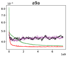
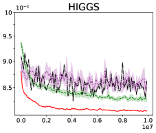
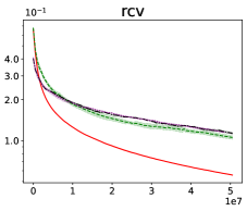
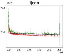
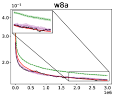
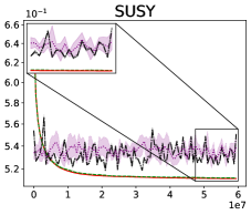
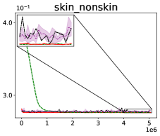
Figure 1: We assess the convergence performance of four algorithms by plotting the objective function value on the $y$-axis against the number of zeroth-order calls on the $x$-axis.

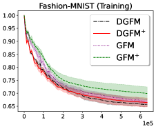
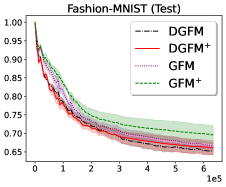
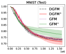
Figure 2: We assess the attacking performance of four algorithms by plotting the accuracy after attacking on the $y$-axis against the number of zeroth-order calls on the $x$-axis.

5.2 Universal Attack

We consider the black-box adversarial attack on image classification with LeNet (LeCun et al., 1998). Our objective is to discover a universal adversarial perturbation (Moosavi-Dezfooli et al., 2017). When applied to the original image, this perturbation induces misclassification in machine learning models while remaining inconspicuous to human observers. Network topology and Performance measures are the same as in the previous experiment. However, we set $m=8$ for two decentralized algorithms here.

Dataset	Fashion-MNIST		MNIST
	Training	Test	Training	Test
DGFM	65.66(0.88)	65.22(1.07)	71.92(1.56)	73.18(1.21)
DGFM+	66.46(1.80)	66.14(2.03)	70.62(2.47)	71.42(2.50)
GFM	66.86(0.90)	66.64(1.02)	73.20(0.41)	73.66(0.55)
GFM+	69.92(2.67)	69.62(2.63)	76.64(3.29)	77.52(3.29)

Table 2: Attacking result (Accuracy/std%)

Data:

We evaluate our proposed algorithms using two standard datasets, MNIST and Fashion-MNIST.

Model:

The problem can be formulated as the following nonsmooth nonconvex problem:

$$\min_{\|\zeta\|_{\infty}\leq\kappa}\frac{1}{m}\sum_{i=1}^{m}\bigg{(}\frac{1}{|\mathcal{D}_{i}|}\sum_{j=1}^{|\mathcal{D}_{i}|}-\ell(a_{i}^{j}+\zeta,b_{i}^{j})\bigg{)},$$

where the dataset $\mathcal{D}_{i}=\{a_{i}^{j},b_{i}^{j}\}$, $a_{i}^{j}$ represents the image features, $b_{i}^{j}\in\mathbb{R}^{C}$ is the one-hot encoding label, $C$ is the number of classes, $|\mathcal{D}_{i}|$ is the cardinality of dataset $\mathcal{D}_{i}$, $\kappa$ is the constraint level of the distortion, $\zeta$ is the perturbation vector and $\ell(\cdot,\cdot)$ is the cross entropy function. We set $\kappa=0.25$ for Fashion-MNIST and $\kappa=0.5$ for MNIST. Following the setup in the work of Chen et al. (2023), we iteratively perform an additional projection step for constraint satisfaction.

Comparison:

We use two pre-trained models with 99.29% accuracy on MNIST and 92.30% accuracy on Fashion-MNIST, respectively. We use GFM, GFM⁺, DGFM and DGFM⁺ to attack the pre-trained LeNet on $59577$ images of MNIST and $55384$ images of Fashion-MNIST, which are classified correctly on the train set for training LeNet. Furthermore, we evaluate the perturbation on a dataset comprising 9885 MNIST images and 8975 Fashion-MNIST images. These images have been accurately classified during the testing phase of the LetNet training. Throughout all the experiments, we set $\delta=0.01$, $b=\{16,32,64\}$. For DGFM⁺ and GFM⁺, we tune $b^{\prime}$ from $\{40,80,800,1600\}$, $T$ from $\{2,5,10,20\}$. Additionally, tune $\mathcal{T}$ from $\{1,10,20\}$ for DGFM⁺. For all algorithms, we tune the stepsize $\eta$ from $\{0.05,0.1,0.5,1\}$ and multiply a decay factor $0.6$ if no improvement in $300$ iterations. For all experiments, we set the initial perturbation as $\mathbf{0}$. The results of the average of five runs are shown in Figure 2 and Table 2. On the Fashion-MNIST dataset, DGFM achieves the lowest accuracy after attacking and small variance. For MNIST, DGFM⁺ achieves the lowest accuracy after attacking, but its variance is larger. In general, we can observe that our algorithms perform better than the serial counterparts.

6 Conclusion

We proposed the first decentralized gradient-free algorithm which has a provable complexity guarantee for non-smooth non-convex optimization over a multi-agent network. We showed that this method obtains an $\mathcal{O}(d^{3/2}\delta^{-1}\varepsilon^{-4})$ complexity for obtaining an $\mathcal{O}(\delta,\varepsilon)$-Goldstein stationary point. Further, we introduced a decentralized variance-reduced method that enhances the complexity to $\mathcal{O}(d^{3/2}\delta^{-1}\varepsilon^{-3})$, thereby achieving the best complexity rate for non-smooth and non-convex optimization in the serial setting. As a future direction, it would be interesting to investigate whether the best complexity bound can be further improved. Additionally, expanding our algorithms to accommodate more challenging scenarios, such as asynchronous distributed optimization, presents an intriguing avenue for further exploration.

Appendix

 

[appendix] [appendix]1

 

In the appendix, we compile a comprehensive list of all Propositions, Lemmas, and Theorems mentioned in the paper, along with their proofs, for improved readability of the main text. We also restate these results in the appendix.

To further support the proof of Lemma C.5 and D.7, we provide the following auxiliary lemmas which are not mentioned in the main text: Lemma C.4 in Section C.4 and Lemma D.6 in Section D.5.

To facilitate the understanding of our proofs, we first present two algorithms in Section A. We then introduce the notation used in the proof and a frequently used proposition in Section B. The proofs of the convergence of DGFM and DGFM⁺ can be found in Sections C and D, respectively. To illustrate the practicality and effectiveness of our algorithms, we also provide specific examples of parameters for both algorithms that can lead to the optimal convergence rate.

Appendix A Algorithms

We give the two decentralized algorithms here for completeness.

Algorithm 3 DGFM at each node $i$

1:$x_{i}^{-1}=x_{i}^{0}=\bar{x}^{0},\forall i\in[m]$, $y_{i}^{0}=g_{i}(x_{i}^{-1};S_{i}^{-1})=\mathbf{0}_{d},K,\eta$

2:for $k=0,\ldots,K-1$ do

3:     Sample $S_{i}^{k}=\big{\{}\xi_{i}^{k,1},w_{i}^{k,1}\big{\}}$ and calculate $g_{i}(x_{i}^{k};S_{i}^{k})$

4:     $y_{i}^{k+1}=\sum_{j=1}^{m}a_{i,j}(k)(y_{j}^{k}+g_{j}(x_{j}^{k};S_{j}^{k})-g_{j}(x_{j}^{k-1};S_{j}^{k-1}))$

5:     $x_{i}^{k+1}={\textstyle{\sum}}_{j=1}^{m}a_{i,j}(k)(x_{j}^{k}-\eta y_{j}^{k+1})$

6:end for

7:Return: Choose $x_{\text{out}}$ uniformly at random from $\big{\{}{x}^{k}_{i}\big{\}}_{k=1,\cdots,K,i=1,\cdots,m}$

Algorithm 4 DGFM⁺ at each node $i$

1:$x_{i}^{-1}=x_{i}^{0}=\bar{x}^{0},\forall i\in[m]$, $y_{i}^{0}=v_{i}^{-1}=\mathbf{0}_{d},K,\eta,b,b^{\prime}$

2:for $k=0,\ldots,K-1$ do

3:     if $k$ mod $T$ = 0 then

4:         Sample $S_{i}^{k\prime}=\big{\{}(\xi_{i}^{k\prime,j},w_{i}^{k\prime,j})\big{\}}_{j=1}^{b^{\prime}}$

5:         Calculate $y_{i}^{k+1}=v_{i}^{k}=g_{i}(x_{i}^{k};S_{i}^{k})$

6:         for $\tau=1,\cdots,\mathcal{T}$ do

7:              $y_{i}^{k+1}={\textstyle{\sum}}_{j=1}^{m}a_{i,j}^{\tau}(k)y_{j}^{k+1}$

8:         end for

9:     else

10:         Sample $S_{i}^{k}=\big{\{}(\xi_{i}^{k,j},w_{i}^{k,j})\big{\}}_{j=1}^{b}$

11:         $v_{i}^{k}=v_{i}^{k-1}+g_{i}(x_{i}^{k};S_{i}^{k})-g_{i}(x_{i}^{k-1};S_{i}^{k})$

12:         $y_{i}^{k+1}={\textstyle{\sum}}_{j=1}^{m}a_{i,j}(k)(y_{j}^{k}+v_{j}^{k}-v_{j}^{k-1})$

13:     end if

14:     $x_{i}^{k+1}={\textstyle{\sum}}_{j=1}^{m}a_{i,j}(k)(x_{j}^{k}-\eta y_{j}^{k+1})$

15:end for

16:Return: Choose $x_{\text{out}}$ uniformly at random from $\big{\{}{x}^{k}_{i}\big{\}}_{k=1,\cdots,K,i=1,\cdots,m}$

Appendix B Preliminaries

In this section, we introduce the notations listed in Table 3, which will be used consistently throughout the document. We also provide a commonly used proposition, Proposition B.1, along with its proof for easy reference.

Table 3: Notations for DGFM and DGFM⁺

Notations	Specific Formulation	Specific Meaning	Dimension
$\mathbf{x}^{k}$	$[(x_{1}^{k})^{\top},\cdots,(x_{m}^{k})^{\top}]^{\top}$	Stack all local variables $x_{i}^{k}$	$\mathbb{R}^{md}$
$\tilde{\mathbf{x}}^{k}$	$[(\tilde{x}_{1}^{k})^{\top},\cdots,(\tilde{x}_{m}^{k})^{\top}]^{\top}$	Stack all local variables $\tilde{x}_{i}^{k}$	$\mathbb{R}^{md}$
$\bar{\mathbf{x}}^{k}$	$\mathbf{1}_{m}\otimes\bar{x}^{k}$	Copy variable $\bar{x}^{k}$ and concatenate	$\mathbb{R}^{md}$
$\mathbf{y}^{k}$	$[(y_{1}^{k})^{\top},\cdots,(y_{m}^{k})^{\top}]^{\top}$	Stack all local variables $y_{i}^{k}$	$\mathbb{R}^{md}$
$\bar{\mathbf{y}}^{k}$	$\mathbf{1}_{m}\otimes\bar{y}^{k}$	Copy variable $\bar{y}^{k}$ and concatenate	$\mathbb{R}^{md}$
$\mathbf{v}^{k}$	$[(v_{1}^{k})^{\top},\cdots,(v_{m}^{k})^{\top}]^{\top}$	Stack all local variables $v_{i}^{k}$	$\mathbb{R}^{md}$
$\bar{\mathbf{v}}^{k}$	$\mathbf{1}_{m}\otimes\bar{v}^{k}$	Copy variable $\bar{v}^{k}$ and concatenate	$\mathbb{R}^{md}$
$\tilde{A}(k)$	$A(k)\otimes\mathbf{I}_{d}$	Doubly Stochastic Matrix for nodes	$\mathbb{R}^{md\times md}$
$J$	$\frac{1}{m}\mathbf{1}_{m}\mathbf{1}_{m}^{\top}\otimes\mathbf{I}_{d}$	Mean Matrix	$\mathbb{R}^{md\times md}$
$\mathbf{g}(\mathbf{x}^{k};S^{k})$	$[(g_{1}(x_{1}^{k};S_{1}^{k}))^{\top},\cdots,(g_{m}(x_{m}^{k};S_{m}^{k}))^{\top}]^{\top}$	Stack all local variables $g(x_{i}^{k};S_{i}^{k})$	$\mathbb{R}^{md}\to\mathbb{R}^{md}$
$\nabla f_{\delta}^{i}(x)$	$\mathbb{E}_{\xi}[\nabla f_{\delta}^{i}(x;\xi)]=\mathbb{E}_{S_{i}}[g(x_{i};S_{i})]$	Expectation of stochastic gradient	$\mathbb{R}^{d}\to\mathbb{R}^{d}$

Proposition B.1

Let $\tilde{A}(k)=A(k)\otimes\mathbf{I}_{d}$ and $J=\frac{1}{m}\mathbf{1}_{m}\mathbf{1}_{m}^{\top}\otimes\mathbf{I}_{d}$, then we have

1. $\tilde{A}(k)J=J=J\tilde{A}(k)$.

2. $\tilde{A}(k)\bar{\mathbf{z}}^{k}=\bar{\mathbf{z}}^{k}=J\bar{\mathbf{z}}^{k},\forall\bar{z}^{k}\in\mathbb{R}^{d}$.

3. There exists a constant $\rho>0$ such that $\max_{k}\{\big{\|}\tilde{A}(k)-J\big{\|}\}\leq\rho<1$.

4. $\big{\|}\tilde{A}(k)\big{\|}\leq 1$.

Proof. First, we have

$$\tilde{A}(k)J=(A(k)\otimes\mathbf{I}_{m})\cdot(\frac{1}{m}\mathbf{1}_{m}\mathbf{1}_{m}^{\top}\otimes\mathbf{I}_{m})=(\frac{1}{m}A(k)\mathbf{1}_{m}\mathbf{1}_{m}^{\top}\otimes\mathbf{I}_{m})\overset{(a)}{=}\frac{1}{m}\mathbf{1}_{m}\mathbf{1}_{m}^{T}\otimes\mathbf{I}_{m}=J\overset{(b)}{=}J\tilde{A}(k),$$

where $(a)$ holds by doubly stochasticity and $(b)$ follows from the similar argument in above $\tilde{A}(k)J=J$ based on $\mathbf{1}_{m}^{\top}\tilde{A}(k)=\mathbf{1}_{m}^{\top}$.

Second, it follows from $\bar{\mathbf{z}}^{k}=\mathbf{1}\otimes\bar{z}^{k}$ that

$$\tilde{A}(k)\bar{\mathbf{z}}^{k}=(A(k)\otimes\mathbf{I}_{d})(\mathbf{1}\otimes\bar{z}^{k})=\mathbf{1}\otimes\bar{z}^{k}=\bar{\mathbf{z}}^{k}=(\frac{1}{m}\mathbf{1}_{m}\mathbf{1}_{m}^{\top}\otimes\mathbf{I}_{d})\otimes(\mathbf{1}\otimes\bar{z}^{k})=J\bar{\mathbf{z}}^{k}.$$

Third, $\big{\|}\tilde{A}(k)-J\big{\|}\leq\rho$ is a well known conclusion (see e.g., Tsitsiklis [1984]).

Last, $\big{\|}\tilde{A}(k)\big{\|}\leq 1$ is a well known result (see e.g., Sun et al. [2022]). $\Box$

Appendix C Convergence Analysis for DGFM

In this section, we present the proofs for the lemmas and theorems that are used in the convergence analysis of the DGFM algorithm.

C.1 Proof of Lemma 3.1

Lemma C.1

Let $\{x_{i}^{k},y_{i}^{k},g_{i}(x_{i}^{k};S_{i}^{k})\}$ be the sequence generated by DGFM and $\{\mathbf{x}^{k},\mathbf{y}^{k},\mathbf{g}^{k}\}$ be the corresponding stack variables, then for $k\geq 0$, we have

$$\mathbf{x}^{k+1} =\tilde{A}(k)(\mathbf{x}^{k}-\eta\mathbf{y}^{k+1}),$$ (C.1)

$$\mathbf{y}^{k+1} =\tilde{A}(k)(\mathbf{y}^{k}+\mathbf{g}^{k}-\mathbf{g}^{k-1}),$$ (C.2)

$$\bar{\mathbf{x}}^{k+1} =\bar{\mathbf{x}}^{k}-\eta\bar{\mathbf{y}}^{k+1},$$ (C.3)

$$\bar{\mathbf{y}}^{k+1} =\bar{\mathbf{y}}^{k}+\bar{\mathbf{g}}^{k}-\bar{\mathbf{g}}^{k-1},$$ (C.4)

$$\bar{\mathbf{y}}^{k+1} =\bar{\mathbf{g}}^{k}.$$ (C.5)

Proof. It follows from $x_{i}^{k+1}=\sum_{j=1}^{m}a_{i,j}(k)(x_{j}^{k}-\eta y_{j}^{k+1})$ and the definition of $\tilde{A}(k)$, $\mathbf{x}^{k}$ and $\mathbf{y}^{k}$ that (C.1). Similar result (C.2) holds by $y_{i}^{k+1}=\sum_{j=1}^{m}a_{i,j}(k)(y_{j}^{k}+g_{j}^{k}-g_{j}^{k-1})$. It follows from $J\tilde{A}(k)=J$ in 1 of Proposition B.1, (C.1) and (C.2) that (C.3) and (C.4) hold. Furthermore, combining $y_{i}^{0}=g_{i}^{-1}=\mathbf{0}_{d}$ and (C.4) yields (C.5). $\Box$

C.2 Proof of Lemma 3.2

Lemma C.2 (Consensus error decay)

Let $\{\bar{\mathbf{x}}^{k},\bar{\mathbf{y}}^{k}\}$ be the sequence generated by DGFM, then for $k\geq 0$, we have

$$\mathbb{E}\big{[}\big{\|}\mathbf{x}^{k+1}-\bar{\mathbf{x}}^{k+1}\big{\|}^{2}\big{]}$$ (C.6)

$$\leq\ \rho^{2}(1+\alpha_{1})\mathbb{E}\big{[}\big{\|}\mathbf{x}^{k}-\bar{\mathbf{x}}^{k}\big{\|}^{2}\big{]}+\rho^{2}\eta^{2}(1+\alpha_{1}^{-1})\mathbb{E}\big{[}\big{\|}\mathbf{y}^{k+1}-\bar{\mathbf{y}}^{k+1}\big{\|}^{2}\big{]},$$

and

$$\mathbb{E}\big{[}\big{\|}\mathbf{y}^{k+1}-\bar{\mathbf{y}}^{k+1}\big{\|}^{2}\mid\mathcal{F}_{k}\big{]}$$ (C.7)

$$\leq\ \rho^{2}(1+\alpha_{2})\mathbb{E}\big{[}\big{\|}\mathbf{y}^{k}-\bar{\mathbf{y}}^{k}\big{\|}^{2}\mid\mathcal{F}_{k}\big{]}+\rho^{2}(1+\alpha_{2}^{-1})(6+36{\eta^{2}}L_{\delta}^{2})m\sigma^{2}$$

$$\ \ +9\rho^{2}(1+\alpha_{2}^{-1})L_{\delta}^{2}\mathbb{E}\big{[}\big{\|}\mathbf{x}^{k}-\bar{\mathbf{x}}^{k}\big{\|}^{2}\mid\mathcal{F}_{k}\big{]}$$

$$\ \ +9\rho^{2}(1+\alpha_{2}^{-1}L_{\delta}^{2}(1+4\eta^{2}L_{\delta}^{2})\mathbb{E}\big{[}\big{\|}\mathbf{x}^{k-1}-\bar{\mathbf{x}}^{k-1}\big{\|}^{2}\mid\mathcal{F}_{k}\big{]}$$

$$\ \ +18L_{\delta}^{2}\eta^{2}{\rho^{2}}(1+\alpha_{2}^{-1})\mathbb{E}\big{[}\big{\|}\nabla f_{\delta}(\bar{x}^{k-1})\big{\|}^{2}\mid\mathcal{F}_{k}\big{]}.$$

Proof. We consider sequence $\{\mathbf{x}^{k}\},\{\mathbf{y}^{k}\}$, separately.

Sequence $\{\mathbf{x}^{k}\}$: It follows from (C.1) that

$$\mathbf{x}^{k+1}-\bar{\mathbf{x}}^{k+1}=(\tilde{A}(k)-J)(\mathbf{x}^{k}-\eta\mathbf{y}^{k+1}).$$

Combining the above inequality and (2), (3) in Proposition B.1, we have

$$\big{\|}\mathbf{x}^{k+1}-\bar{\mathbf{x}}^{k+1}\big{\|} \leq\rho\big{\|}\mathbf{x}^{k}-\bar{\mathbf{x}}^{k}\big{\|}+\rho\eta\big{\|}\mathbf{y}^{k+1}-\bar{\mathbf{y}}^{k+1}\big{\|}.$$

Combining the above inequality and Young’s inequality and taking the expectation, then we complete the proof of (C.6).

Sequence $\{\mathbf{y}^{k}\}$: It follows from (C.2) that $\big{\|}\mathbf{y}^{k+1}-\bar{\mathbf{y}}^{k+1}\big{\|}\leq\rho\big{\|}\mathbf{y}^{k}-\bar{\mathbf{y}}^{k}\big{\|}+\rho\big{\|}\mathbf{g}^{k}-\mathbf{g}^{k-1}\big{\|}.$ Combining the above inequality, Young’s inequality, and taking the expectation on natural field $\mathcal{F}_{k}$, then we have

$$\mathbb{E}\big{[}\big{\|}\mathbf{y}^{k+1}-\bar{\mathbf{y}}^{k+1}\big{\|}^{2}\mid\mathcal{F}_{k}\big{]} \leq\rho^{2}(1+\alpha_{2})\mathbb{E}\big{[}\big{\|}\mathbf{y}^{k}-\bar{\mathbf{y}}^{k}\big{\|}^{2}\mid\mathcal{F}_{k}\big{]}+\rho^{2}(1+\alpha_{2}^{-1})\mathbb{E}\big{[}\big{\|}\mathbf{g}^{k}-\mathbf{g}^{k-1}\big{\|}^{2}\mid\mathcal{F}_{k}\big{]}.$$

Note that

$$\mathbb{E}\big{[}\big{\|}\mathbf{g}^{k}-\mathbf{g}^{k-1}\big{\|}^{2}\mid\mathcal{F}_{k}\big{]} =\sum_{i=1}^{m}\mathbb{E}\big{[}\big{\|}g_{i}(x_{i}^{k};S_{i}^{k})\pm\nabla f_{\delta}^{i}(x_{i}^{k})\pm\nabla f_{\delta}^{i}(x_{i}^{k-1})-g_{i}(x_{i}^{k};S_{i}^{k-1})\big{\|}^{2}\mid\mathcal{F}_{k}\big{]}$$

$$\leq 3\sum_{i=1}^{m}\left(2\sigma^{2}+L_{\delta}^{2}\mathbb{E}\big{[}\big{\|}x_{i}^{k}-x_{i}^{k-1}\big{\|}^{2}\mid\mathcal{F}_{k}\big{]}\right)$$

$$=6m\sigma^{2}+3L_{\delta}^{2}\mathbb{E}\big{[}\big{\|}\mathbf{x}^{k}-\mathbf{x}^{k-1}\big{\|}^{2}\mid\mathcal{F}_{k}\big{]}$$

$$\leq 6m\sigma^{2}+9L_{\delta}^{2}\big{(}\mathbb{E}\big{[}\big{\|}\mathbf{x}^{k}-\bar{\mathbf{x}}^{k}\big{\|}^{2}+\big{\|}\bar{\mathbf{x}}^{k}-\bar{\mathbf{x}}^{k-1}\big{\|}^{2}+\big{\|}\mathbf{x}^{k-1}-\bar{\mathbf{x}}^{k-1}\big{\|}^{2}\mid\mathcal{F}_{k}\big{]}\big{)}$$

$$=6m\sigma^{2}+9L_{\delta}^{2}\big{(}\mathbb{E}\big{[}\big{\|}\mathbf{x}^{k}-\bar{\mathbf{x}}^{k}\big{\|}^{2}+\eta^{2}\big{\|}\bar{\mathbf{y}}^{k}\big{\|}^{2}+\big{\|}\mathbf{x}^{k-1}-\bar{\mathbf{x}}^{k-1}\big{\|}^{2}\mid\mathcal{F}_{k}\big{]}\big{)},$$

and

$$\mathbb{E}\big{[}\big{\|}\bar{\mathbf{y}}^{k}\big{\|}^{2}\mid\mathcal{F}_{k}\big{]}$$

$$\leq m\cdot\mathbb{E}\bigg{[}2\Big{\|}\frac{1}{m}\sum_{i=1}^{m}(g_{i}(x_{i}^{k-1};S_{i}^{k-1})\pm\nabla f_{\delta}^{i}(x_{i}^{k-1})-\nabla f_{\delta}^{i}(\bar{x}^{k-1})\Big{\|}^{2}+2\Big{\|}\frac{1}{m}\sum_{i=1}^{m}\nabla f_{\delta}^{i}(\bar{x}^{k-1})\Big{\|}^{2}\mid\mathcal{F}_{k}\bigg{]}$$

$$\ \ +4m\mathbb{E}\bigg{[}\Big{\|}\frac{1}{m}\sum_{i=1}^{m}f_{\delta}^{i}(x_{i}^{k-1})-\nabla f_{\delta}^{i}(\bar{x}^{k-1})\Big{\|}^{2}\mid\mathcal{F}_{k}\bigg{]}+2\mathbb{E}\big{[}\big{\|}\nabla f_{\delta}(\bar{x}^{k-1})\big{\|}^{2}\mid\mathcal{F}_{k}\big{]}$$

$$\leq 4\mathbb{E}\bigg{[}\sum_{i=1}^{m}\big{\|}g_{i}(x_{i}^{k-1};S_{i}^{k-1})-\nabla f_{\delta}^{i}(x_{i}^{k-1})\big{\|}^{2}\bigg{]}+4\mathbb{E}\bigg{[}\sum_{i=1}^{m}\big{\|}\nabla f_{\delta}^{i}(x_{i}^{k-1})-\nabla f_{\delta}^{i}(\bar{x}^{k-1})\big{\|}^{2}\mid\mathcal{F}_{k}\bigg{]}$$

$$\ \ +2\mathbb{E}\big{[}\big{\|}\nabla f_{\delta}(\bar{x}^{k-1})\big{\|}^{2}\mid\mathcal{F}_{k}\big{]}$$

$$\leq 4m\sigma^{2}+4L_{\delta}^{2}\mathbb{E}\big{[}\big{\|}\mathbf{x}^{k-1}-\bar{\mathbf{x}}^{k-1}\big{\|}^{2}\mid\mathcal{F}_{k}\big{]}+2\mathbb{E}\big{[}\big{\|}\nabla f_{\delta}(\bar{x}^{k-1})\big{\|}^{2}\mid\mathcal{F}_{k}\big{]}.$$

Combining the above three inequalities and taking expectation with all random variables yield

$$\mathbb{E}\big{[}\big{\|}\mathbf{y}^{k+1}-\bar{\mathbf{y}}^{k+1}\big{\|}^{2}\mid\mathcal{F}_{k}\big{]}$$

$$\leq\rho^{2}(1+\alpha_{2})\mathbb{E}\big{[}\big{\|}\mathbf{y}^{k}-\bar{\mathbf{y}}^{k}\big{\|}^{2}\mid\mathcal{F}_{k}\big{]}+\rho^{2}(1+\alpha_{2}^{-1})\mathbb{E}\big{[}\big{\|}\mathbf{g}^{k}-\mathbf{g}^{k-1}\big{\|}^{2}\mid\mathcal{F}_{k}\big{]}$$

$$\leq\rho^{2}(1+\alpha_{2})\mathbb{E}\big{[}\big{\|}\mathbf{y}^{k}-\bar{\mathbf{y}}^{k}\big{\|}^{2}\mid\mathcal{F}_{k}\big{]}$$

$$\ \ +\rho^{2}(1+\alpha_{2}^{-1})\left(6m\sigma^{2}+9L_{\delta}^{2}(\mathbb{E}\big{[}\big{\|}\mathbf{x}^{k}-\bar{\mathbf{x}}^{k}\big{\|}^{2}+\eta^{2}\big{\|}\bar{\mathbf{y}}^{k}\big{\|}^{2}+\big{\|}\mathbf{x}^{k-1}-\bar{\mathbf{x}}^{k-1}\big{\|}^{2}\mid\mathcal{F}_{k}\big{]})\right)$$

$$\leq\rho^{2}(1+\alpha_{2})\mathbb{E}\big{[}\big{\|}\mathbf{y}^{k}-\bar{\mathbf{y}}^{k}\big{\|}^{2}\mid\mathcal{F}_{k}\big{]}$$

$$\ \ +\rho^{2}(1+\alpha_{2}^{-1})\left(6m\sigma^{2}+9L_{\delta}^{2}(\mathbb{E}\big{[}\big{\|}\mathbf{x}^{k}-\bar{\mathbf{x}}^{k}\big{\|}^{2}+\big{\|}\mathbf{x}^{k-1}-\bar{\mathbf{x}}^{k-1}\big{\|}^{2}\mid\mathcal{F}_{k}\big{]})\right.$$

$$\ \ \left.+9L_{\delta}^{2}\eta^{2}(4m\sigma^{2}+4L_{\delta}^{2}\mathbb{E}\big{[}\big{\|}\mathbf{x}^{k-1}-\bar{\mathbf{x}}^{k-1}\big{\|}^{2}\mid\mathcal{F}_{k}\big{]}+2\mathbb{E}\big{[}\big{\|}\nabla f_{\delta}(\bar{x}^{k-1})\big{\|}^{2}\mid\mathcal{F}_{k}\big{]}\right)$$

$$=\rho^{2}(1+\alpha_{2})\cdot\mathbb{E}\big{[}\big{\|}\mathbf{y}^{k}-\bar{\mathbf{y}}^{k}\big{\|}^{2}\mid\mathcal{F}_{k}\big{]}+\rho^{2}(1+\alpha_{2}^{-1})(6+36{\eta^{2}}L_{\delta}^{2})m\sigma^{2}$$

$$\ \ +9\rho^{2}(1+\alpha_{2}^{-1})L_{\delta}^{2}\cdot\mathbb{E}\big{[}\big{\|}\mathbf{x}^{k}-\bar{\mathbf{x}}^{k}\big{\|}^{2}\mid\mathcal{F}_{k}\big{]}$$

$$\ \ +9\rho^{2}(1+\alpha_{2}^{-1}L_{\delta}^{2}(1+4\eta^{2}L_{\delta}^{2})\cdot\mathbb{E}\big{[}\big{\|}\mathbf{x}^{k-1}-\bar{\mathbf{x}}^{k-1}\big{\|}^{2}\mid\mathcal{F}_{k}\big{]}$$

$$\ \ +18L_{\delta}^{2}\eta^{2}{\rho^{2}}(1+\alpha_{2}^{-1})\cdot\mathbb{E}\big{[}\big{\|}\nabla f_{\delta}(\bar{x}^{k-1})\big{\|}^{2}\mid\mathcal{F}_{k}\big{]},$$

which complete the proof of (C.7). $\Box$

C.3 Proof of Lemma 3.3

Lemma C.3 (Descent Property of DGFM)

Let $\{\mathbf{x}^{k},\mathbf{y}^{k},\bar{\mathbf{x}}^{k},\bar{\mathbf{y}}^{k}\}$ be the sequence generated by DGFM, then we have

$$\mathbb{E}\big{[}f_{\delta}(\bar{x}^{k+1})\big{]}-\mathbb{E}\big{[}f_{\delta}(\bar{x}^{k})\big{]}\leq-\frac{\eta}{2}\mathbb{E}\big{[}\big{\|}\nabla f_{\delta}(\bar{x}^{k})\big{\|}^{2}\big{]}+\frac{\eta L_{\delta}^{2}}{2m}\mathbb{E}\big{[}\big{\|}\mathbf{x}^{k}-\bar{\mathbf{x}}^{k}\big{\|}^{2}\big{]}+L_{\delta}\eta^{2}(\sigma^{2}+L_{f}^{2}).$$ (C.8)

Proof. It follows from $f_{\delta}^{i}(x)$ is differentiable and $L_{f}$-Lipschitz with $L_{\delta}$-Lipschitz gradient that

$$f_{\delta}^{i}(\bar{x}^{k+1}) \leq f_{\delta}^{i}(\bar{x}^{k})-\big{\langle}\nabla f_{\delta}^{i}(\bar{x}^{k}),\bar{x}^{k+1}-\bar{x}^{k}\big{\rangle}+\frac{L_{\delta}}{2}\big{\|}\bar{x}^{k+1}-\bar{x}^{k}\big{\|}^{2}$$

$$=f_{\delta}^{i}(\bar{x}^{k})-\eta\big{\langle}\nabla f_{\delta}^{i}(\bar{x}^{k}),\bar{g}^{k}\big{\rangle}+\frac{L_{\delta}\eta^{2}}{2}\big{\|}\bar{g}^{k}\big{\|}^{2}.$$

Summing the above inequality over $i=1$ to $m$, dividing by $m$ and taking expectation on $\mathcal{F}_{k}$, then we have

$$\mathbb{E}\big{[}f_{\delta}(\bar{x}^{k+1})\mid\mathcal{F}_{k}\big{]}\leq f_{\delta}(\bar{x}^{k})-\eta\big{\langle}\nabla f_{\delta}(\bar{x}^{k}),\mathbb{E}\big{[}\bar{g}^{k}\mid\mathcal{F}_{k}\big{]}\big{\rangle}+\frac{L_{\delta}\eta^{2}}{2}\mathbb{E}\big{[}\big{\|}\bar{g}^{k}\big{\|}^{2}\mid\mathcal{F}_{k}\big{]}.$$ (C.9)

By $\mathbb{E}\left[\bar{g}^{k}\mid\mathcal{F}_{k}\right]=\frac{1}{m}\sum_{i=1}^{m}\nabla f_{\delta}^{i}(x_{i}^{k})$ and the above inequality, we have

$$\big{\langle}\nabla f_{\delta}(\bar{x}^{k}),\mathbb{E}\big{[}\bar{g}^{k}\mid\mathcal{F}_{k}\big{]}\big{\rangle} =\Big{\langle}\nabla f_{\delta}(\bar{x}^{k}),\frac{1}{m}\sum_{i=1}^{m}\nabla f_{\delta}^{i}(x_{i}^{k})-\nabla f_{\delta}(\bar{x}^{k})\Big{\rangle}+\big{\|}\nabla f_{\delta}(\bar{x}^{k})\big{\|}^{2}$$ (C.10)

$$\mathbb{E}\big{[}\big{\|}\bar{g}^{k}\big{\|}^{2}\mid\mathcal{F}_{k}\big{]} \leq 2\mathbb{E}\bigg{[}\Big{\|}\bar{g}^{k}-\frac{1}{m}\sum_{i=1}^{m}\nabla f_{\delta}^{i}(x_{i}^{k})\Big{\|}^{2}+2\Big{\|}\frac{1}{m}\sum_{i=1}^{m}\nabla f_{\delta}^{i}(x_{i}^{k})\Big{\|}^{2}\mid\mathcal{F}_{k}\bigg{]}$$ (C.11)

$$\leq 2(\sigma^{2}+L_{f}^{2}),$$

Combining (C.9), (C.10) and (C.11) yields

$$\mathbb{E}\big{[}f_{\delta}(\bar{x}^{k+1})\mid\mathcal{F}_{k}\big{]}$$

$$\leq\mathbb{E}\Big{[}f_{\delta}(\bar{x}^{k})-\eta\Big{(}\Big{\langle}\nabla f_{\delta}(\bar{x}^{k}),\frac{1}{m}\sum_{i=1}^{m}\nabla f_{\delta}^{i}(x_{i}^{k})-\nabla f_{\delta}(\bar{x}^{k})\Big{\rangle}+\big{\|}\nabla f_{\delta}(\bar{x}^{k})\big{\|}^{2}\Big{)}\mid\mathcal{F}_{k}\Big{]}+L_{\delta}\eta^{2}(\sigma^{2}+L_{f}^{2})$$

$$\overset{(a)}{\leq}\mathbb{E}\bigg{[}f_{\delta}(\bar{x}^{k})-\eta\big{\|}\nabla f_{\delta}(\bar{x}^{k})\big{\|}^{2}+\frac{\eta}{2}\big{\|}\nabla f_{\delta}(\bar{x}^{k})\big{\|}^{2}+\frac{\eta}{2}\big{\|}\frac{1}{m}\sum_{i=1}^{m}\nabla f_{\delta}^{i}(x_{i}^{k})-\nabla f_{\delta}(\bar{x}^{k})\big{\|}^{2}\mid\mathcal{F}_{k}\bigg{]}$$

$$\ \ +L_{\delta}\eta^{2}(\sigma^{2}+L_{f}^{2})$$

$$\leq\mathbb{E}\bigg{[}f_{\delta}(\bar{x}^{k})-\frac{\eta}{2}\big{\|}\nabla f_{\delta}(\bar{x}^{k})\big{\|}^{2}+\frac{\eta L_{\delta}^{2}}{2m}\big{\|}\mathbf{x}^{k}-\bar{\mathbf{x}}^{k}\big{\|}^{2}\mid\mathcal{F}_{k}\bigg{]}+L_{\delta}\eta^{2}(\sigma^{2}+L_{f}^{2}),$$

where $(a)$ holds by $\big{\langle}\mathbf{a},\mathbf{b}\big{\rangle}\leq\frac{1}{2}\big{\|}\mathbf{a}\big{\|}^{2}+\frac{1}{2}\big{\|}\mathbf{b}\big{\|}^{2}$. Taking the expectation of both sides and rearranging yields

$$\mathbb{E}\big{[}f_{\delta}(\bar{x}^{k+1})\big{]}-\mathbb{E}\big{[}f_{\delta}(\bar{x}^{k})\big{]}\leq-\frac{\eta}{2}\mathbb{E}\big{[}\big{\|}\nabla f_{\delta}(\bar{x}^{k})\big{\|}^{2}\big{]}+\frac{\eta L_{\delta}^{2}}{2m}\mathbb{E}\big{[}\big{\|}\mathbf{x}^{k}-\bar{\mathbf{x}}^{k}\big{\|}^{2}\big{]}+L_{\delta}\eta^{2}(\sigma^{2}+L_{f}^{2}).$$

$\Box$

C.4 Proof of Lemma 3.4

Lemma C.4

Let $\{\mathbf{x}^{k},\mathbf{y}^{k},\bar{\mathbf{x}}^{k},\bar{\mathbf{y}}^{k}\}$ be the sequence generated by DGFM, then we have

$$\beta_{x}\mathbb{E}\big{[}\big{\|}\mathbf{x}^{k+1}-\bar{\mathbf{x}}^{k+1}\big{\|}^{2}-\big{\|}\mathbf{x}^{k}-\bar{\mathbf{x}}^{k}\big{\|}^{2}\big{]}+\beta_{y}\mathbb{E}\big{[}\big{\|}\mathbf{y}^{k+1}-\bar{\mathbf{y}}^{k+1}\big{\|}^{2}-\big{\|}\mathbf{y}^{k}-\bar{\mathbf{y}}^{k}\big{\|}^{2}\big{]}$$ (C.12)

$$\leq-(\beta_{x}(1-\rho^{2}(1+\alpha_{1}))-9\beta_{y}L_{\delta}^{2}\cdot\rho^{2}(1+\alpha_{2}^{-1}))\mathbb{E}\big{[}\big{\|}\mathbf{x}^{k}-\bar{\mathbf{x}}^{k}\big{\|}^{2}\big{]}$$

$$\ \ +9\beta_{y}\rho^{2}(1+\alpha_{2}^{-1})L_{\delta}^{2}(1+4\eta^{2}L_{\delta}^{2})\mathbb{E}\big{[}\big{\|}\mathbf{x}^{k-1}-\bar{\mathbf{x}}^{k-1}\big{\|}^{2}\big{]}$$

$$\ \ -\beta_{y}(1-\rho^{2}(1+\alpha_{2}))\mathbb{E}\big{[}\big{\|}\mathbf{y}^{k}-\bar{\mathbf{y}}^{k}\big{\|}^{2}\big{]}+\beta_{x}\rho^{2}\eta^{2}(1+\alpha_{1}^{-1})\mathbb{E}\big{[}\big{\|}\mathbf{y}^{k+1}-\bar{\mathbf{y}}^{k+1}\big{\|}^{2}\big{]}$$

$$\ \ +18\beta_{y}\eta^{2}{\rho^{2}}L_{\delta}^{2}(1+\alpha_{2}^{-1})\mathbb{E}\big{[}\big{\|}\nabla f_{\delta}(\bar{x}^{k-1})\big{\|}^{2}\big{]}+\beta_{y}\rho^{2}m(1+\alpha_{2}^{-1})(6+36L_{\delta}^{2}{\eta^{2}})\sigma^{2},$$

where $\beta_{x}$ and $\beta_{y}>0$.

Proof. It follows from Lemma C.2 that

$$\beta_{x}\mathbb{E}\big{[}\big{\|}\mathbf{x}^{k+1}-\bar{\mathbf{x}}^{k+1}\big{\|}^{2}-\big{\|}\mathbf{x}^{k}-\bar{\mathbf{x}}^{k}\big{\|}^{2}\big{]}$$ (C.13)

$$\leq\beta_{x}\big{(}\rho^{2}(1+\alpha_{1})-1\big{)}\mathbb{E}\big{[}\big{\|}\mathbf{x}^{k}-\bar{\mathbf{x}}^{k}\big{\|}^{2}\big{]}+\beta_{x}\rho^{2}\eta^{2}(1+\alpha_{1}^{-1})\mathbb{E}\big{[}\big{\|}\mathbf{y}^{k+1}-\bar{\mathbf{y}}^{k+1}\big{\|}^{2}\big{]},$$

and

$$\beta_{y}\mathbb{E}\big{[}\big{\|}\mathbf{y}^{k+1}-\bar{\mathbf{y}}^{k+1}\big{\|}^{2}-\big{\|}\mathbf{y}^{k}-\bar{\mathbf{y}}^{k}\big{\|}^{2}\big{]}$$ (C.14)

$$\leq\beta_{y}\big{(}\rho^{2}(1+\alpha_{2})-1\big{)}\mathbb{E}\big{[}\big{\|}\mathbf{y}^{k}-\bar{\mathbf{y}}^{k}\big{\|}^{2}\big{]}+\beta_{y}\rho^{2}(1+\alpha_{2}^{-1})(6m+36m{\eta^{2}}L_{\delta}^{2})\sigma^{2}$$

$$\ \ +9\beta_{y}\rho^{2}(1+\alpha_{2}^{-1})L_{\delta}^{2}\mathbb{E}\big{[}\big{\|}\mathbf{x}^{k}-\bar{\mathbf{x}}^{k}\big{\|}^{2}\big{]}$$

$$\ \ +9\beta_{y}\rho^{2}(1+\alpha_{2}^{-1})L_{\delta}^{2}(1+4\eta^{2}L_{\delta}^{2})\mathbb{E}\big{[}\big{\|}\mathbf{x}^{k-1}-\bar{\mathbf{x}}^{k-1}\big{\|}^{2}\big{]}$$

$$\ \ +18\beta_{y}\eta^{2}{\rho^{2}}L_{\delta}^{2}(1+\alpha_{2}^{-1})\mathbb{E}\big{[}\big{\|}\nabla f_{\delta}(\bar{x}^{k-1})\big{\|}^{2}\big{]},$$

where $\beta_{x}$ and $\beta_{y}>0$. Summing the two inequalities up yields the result. $\Box$

Lemma C.5 (Convergence Result for DGFM)

Let $\{\mathbf{x}^{k},\mathbf{y}^{k},\bar{\mathbf{x}}^{k},\bar{\mathbf{y}}^{k}\}$ be the sequence generated by DGFM, then for any $\beta_{x},\beta_{y}>0$ we have

$$\beta_{x}\mathbb{E}\big{[}\big{\|}\mathbf{x}^{K}-\bar{\mathbf{x}}^{K}\big{\|}^{2}-\big{\|}\mathbf{x}^{0}-\bar{\mathbf{x}}^{0}\big{\|}^{2}\big{]}+\beta_{y}\mathbb{E}\big{[}\big{\|}\mathbf{y}^{{K+1}}-\bar{\mathbf{y}}^{K+1}\big{\|}^{2}-\big{\|}\mathbf{y}^{{1}}-\bar{\mathbf{y}}^{1}\big{\|}^{2}\big{]}$$

$$\ \ +\mathbb{E}\big{[}f_{\delta}(\bar{x}^{K})\big{]}-\mathbb{E}\big{[}f_{\delta}(\bar{x}^{0})\big{]}$$

$$\leq-\big{(}\frac{\eta}{2}-18\beta_{y}{\rho^{2}}\eta^{2}L_{\delta}^{2}(1+\alpha_{2}^{-1})\big{)}\sum_{k=0}^{K-1}\mathbb{E}\big{[}\big{\|}\nabla f_{\delta}(\bar{x}^{k})\big{\|}^{2}\big{]}$$

$$\ \ -\big{(}\beta_{x}(1-\rho^{2}(1+\alpha_{1}))-9\beta_{y}\rho^{2}(1+\alpha_{2}^{-1})L_{\delta}^{2}(1+4\eta^{2}L_{\delta}^{2})-\frac{\eta L_{\delta}^{2}}{2m}\big{)}\sum_{k=0}^{K-1}\mathbb{E}\big{[}\big{\|}\mathbf{x}^{k}-\bar{\mathbf{x}}^{k}\big{\|}^{2}\big{]}$$

$$\ \ +9\beta_{y}\rho^{2}(1+\alpha_{2}^{-1})L_{\delta}^{2}\sum_{k=1}^{K}\mathbb{E}\big{[}\big{\|}\mathbf{x}^{k}-\bar{\mathbf{x}}^{k}\big{\|}^{2}\big{]}$$

$$\ \ -\big{(}\beta_{y}(1-\rho^{2}(1+\alpha_{2}))-\beta_{x}\eta^{2}\cdot\rho^{2}(1+\alpha_{1}^{-1})\big{)}\sum_{k=1}^{K}\mathbb{E}\big{[}\big{\|}\mathbf{y}^{k}-\bar{\mathbf{y}}^{k}\big{\|}^{2}\big{]}$$

$$\ \ +\big{(}\beta_{y}\rho^{2}(1+\alpha_{2}^{-1})(6m+36m{\eta^{2}}L_{\delta}^{2})\sigma^{2}+L_{\delta}\eta^{2}(\sigma^{2}+L_{f}^{2})\big{)}\cdot K.$$

Proof. Summing the combination of (C.12) and (C.8) from $k=0$ to $K-1$ completes our proof. $\Box$

C.5 Proof of Theorem 3.1

Theorem C.1

DGFM can output a $(\delta,\varepsilon)$-Goldstein stationary point of $f(\cdot)$ in expectation with the total stochastic zeroth-order complexity and total communication complexity at most $\mathcal{O}(\Delta_{\delta}\delta^{-1}\varepsilon^{-4})$ by setting $\alpha_{1}=\alpha_{2}=(1-\rho^{2})(2\rho^{2})^{-1}$, $\delta=\mathcal{O}(\varepsilon)$, $\beta_{x}=\mathcal{O}(\delta^{-1}),\beta_{y}=\mathcal{O}(\varepsilon^{4}\delta)$ and $\eta=\mathcal{O}(\varepsilon^{2}\delta)$. Moreover, a specific example of parameters is given as follows:

$$\beta_{y} =\frac{(1-\rho^{2})\varepsilon^{2}}{384\sigma^{2}\rho^{2}(1+\rho^{2})}\cdot\frac{\eta}{m},\ \ \beta_{x}=\frac{1152\sigma^{2}\rho^{2}(1+\rho^{2})}{(1-\rho^{2})^{2}}\cdot L_{\delta}^{2}\varepsilon^{-2}\beta_{y},$$

$$\eta =\min\left\{\frac{(1-\rho^{2})^{2}}{48\sigma(1+\rho^{2})\rho^{2}}\cdot\varepsilon L_{\delta}^{-1},\frac{1}{32}L_{\delta}^{-1}(\sigma^{2}+L_{f})^{-1}\cdot\varepsilon^{2},\frac{8\sqrt{6m\sigma^{2}}}{\varepsilon L_{\delta}}\right\},$$

then DGFM can output a $(\delta,\varepsilon)$-Goldstein stationary point of $f(\cdot)$ in expectation with the total stochastic zeroth-order complexity and total communication complexity at most

$$\mathcal{O}\left(\max\left\{\Delta_{\delta}\varepsilon^{-4}\delta^{-1}d^{\frac{3}{2}},\frac{(1+L_{f}^{2}/\sigma^{2})(1-\rho^{2})}{m(1+\rho^{2})}\right\}\right).$$

Proof. It follows from Lemma C.5 that

$$\beta_{x}\mathbb{E}\big{[}\big{\|}\mathbf{x}^{K}-\bar{\mathbf{x}}^{K}\big{\|}^{2}-\big{\|}\mathbf{x}^{0}-\bar{\mathbf{x}}^{0}\big{\|}^{2}\big{]}+\beta_{y}\mathbb{E}\big{[}\big{\|}\mathbf{y}^{{K+1}}-\bar{\mathbf{y}}^{K+1}\big{\|}^{2}-\big{\|}\mathbf{y}^{{1}}-\bar{\mathbf{y}}^{1}\big{\|}^{2}\big{]}$$

$$\ \ +\mathbb{E}\big{[}f_{\delta}(\bar{x}^{K})\big{]}-\mathbb{E}\big{[}f_{\delta}(\bar{x}^{0})\big{]}$$

$$\leq-\big{(}\frac{\eta}{2}-18\beta_{y}{\rho^{2}}\eta^{2}L_{\delta}^{2}(1+\alpha_{2}^{-1})\big{)}\sum_{k=0}^{K-1}\mathbb{E}\big{[}\big{\|}\nabla f_{\delta}(\bar{x}^{k})\big{\|}^{2}\big{]}$$

$$\ \ -\big{(}\beta_{x}(1-\rho^{2}(1+\alpha_{1}))-18\beta_{y}\rho^{2}(1+\alpha_{2}^{-1})L_{\delta}^{2}({1}+2\eta^{2}L_{\delta}^{2})-\frac{\eta L_{\delta}^{2}}{2m}\big{)}\sum_{k=1}^{K-1}\mathbb{E}\big{[}\big{\|}\mathbf{x}^{k}-\bar{\mathbf{x}}^{k}\big{\|}^{2}\big{]}$$

$$\ \ -\big{(}\beta_{x}(1-\rho^{2}(1+\alpha_{1}))-9\beta_{y}\rho^{2}(1+\alpha_{2}^{-1})L_{\delta}^{2}(1+4\eta^{2}L_{\delta}^{2})-\frac{\eta L_{\delta}^{2}}{2m}\big{)}\mathbb{E}\big{[}\big{\|}\mathbf{x}^{0}-\bar{\mathbf{x}}^{0}\big{\|}^{2}\big{]}$$

$$\ \ +9\beta_{y}\rho^{2}(1+\alpha_{2}^{-1})L_{\delta}^{2}\mathbb{E}\big{[}\big{\|}\mathbf{x}^{K}-\bar{\mathbf{x}}^{K}\big{\|}^{2}\big{]}$$

$$\ \ -\big{(}\beta_{y}(1-\rho^{2}(1+\alpha_{2}))-\beta_{x}\eta^{2}\cdot\rho^{2}(1+\alpha_{1}^{-1})\big{)}\sum_{k=1}^{K}\mathbb{E}\big{[}\big{\|}\mathbf{y}^{k}-\bar{\mathbf{y}}^{k}\big{\|}^{2}\big{]}$$

$$\ \ +\big{(}\beta_{y}\rho^{2}(1+\alpha_{2}^{-1})(6m+36m{\eta^{2}}L_{\delta}^{2})\sigma^{2}+L_{\delta}\eta^{2}(\sigma^{2}+L_{f}^{2})\big{)}\cdot K.$$

which implies

$$\underbrace{\big{(}\frac{\eta}{2}-18\beta_{y}{\rho^{2}}\eta^{2}L_{\delta}^{2}(1+\alpha_{2}^{-1})\big{)}}_{(\textrm{I})}\sum_{k=0}^{K-1}\mathbb{E}\left[\big{\|}\nabla f_{\delta}(\bar{x}^{k})\big{\|}^{2}\right]$$ (C.15)

$$\overset{(a)}{\leq}-\left(\mathbb{E}\left[f_{\delta}(\bar{x}^{K})\right]-\mathbb{E}\left[f_{\delta}(\bar{x}^{0})\right]\right)+\beta_{y}\rho^{2}(\sigma^{2}+L_{f}^{2})$$

$$\ \ -\big{(}\underbrace{\beta_{x}(1-\rho^{2}(1+\alpha_{1}))-18\beta_{y}\rho^{2}(1+\alpha_{2}^{-1})L_{\delta}^{2}(1+2\eta^{2}L_{\delta}^{2})-\frac{\eta L_{\delta}^{2}}{2m}}_{(\textrm{II})}\big{)}\sum_{k=1}^{K-1}\mathbb{E}\left[\big{\|}\mathbf{x}^{k}-\bar{\mathbf{x}}^{k}\big{\|}^{2}\right]$$

$$\ \ -\big{(}\underbrace{\beta_{x}-9\beta_{y}\rho^{2}(1+\alpha_{2}^{-1})L_{\delta}^{2}}_{(\textrm{III})}\big{)}\mathbb{E}\left[\big{\|}\mathbf{x}^{K}-\bar{\mathbf{x}}^{K}\big{\|}^{2}\right]$$

$$\ \ -\big{(}\underbrace{\beta_{y}(1-\rho^{2}(1+\alpha_{2}))-\beta_{x}\eta^{2}\cdot\rho^{2}(1+\alpha_{1}^{-1})}_{(\textrm{IV})}\big{)}\sum_{k=1}^{K}\mathbb{E}\left[\big{\|}\mathbf{y}^{k}-\bar{\mathbf{y}}^{k}\big{\|}^{2}\right]$$

$$\ \ +\big{(}\underbrace{\beta_{y}\rho^{2}(1+\alpha_{2}^{-1})(6m+36m{\eta^{2}}L_{\delta}^{2}\sigma^{2})}_{(\textrm{V})}+\underbrace{L_{\delta}\eta^{2}(\sigma^{2}+L_{f}^{2})}_{(\textrm{VI})}\big{)}\cdot K.$$

where (a) is by $\mathbb{E}\big{[}\big{\|}\mathbf{y}^{{1}}-\bar{\mathbf{y}}^{1}\big{\|}^{2}\big{]}=\mathbb{E}\big{[}\big{\|}(\tilde{A}(0)-J)(\mathbf{y}^{{0}}+\mathbf{g}^{0}-\mathbf{g}^{-1})\big{\|}^{2}\big{]}=\mathbb{E}\big{[}\big{\|}(\tilde{A}(0)-J)\mathbf{g}^{0}\big{\|}^{2}\big{]}\leq\rho^{2}(\sigma^{2}+L_{f}^{2})$.

By setting $\alpha_{1}=\alpha_{2}=(1-\rho^{2})(2\rho^{2})^{-1}$, we have

$$1-\rho^{2}(1+\alpha_{1})=1-\rho^{2}(1+\alpha_{2})=\frac{1-\rho^{2}}{2},$$

and

$$1+\alpha_{1}^{-1}=1+\alpha_{2}^{-1}=\frac{1+\rho^{2}}{1-\rho^{2}}.$$

Combining the parameters setting of $\beta_{x},\beta_{y}$ and $\eta$ yields $(\textrm{I})$-$(\textrm{VI})>0$ and

$$(\textrm{I})=\mathcal{O}(\varepsilon^{2}\delta),\ (\textrm{II})=\mathcal{O}(\delta^{-1}),\ (\textrm{III})=\mathcal{O}(\delta^{-1}),\ (\textrm{IV})=\mathcal{O}(\varepsilon^{4}\delta),\ (\textrm{V})=\mathcal{O}(\varepsilon^{4}\delta),\ (\textrm{VI})=\mathcal{O}(\varepsilon^{4}\delta).$$ (C.16)

Rearranging (C.15) and combining $(\textrm{III})>(\textrm{II})$ yields

$$(\textrm{I})\sum_{k=0}^{K-1}\mathbb{E}\big{[}\big{\|}\nabla f_{\delta}(\bar{x}^{k})\big{\|}^{2}\big{]}+(\textrm{II})\sum_{k=1}^{K}\mathbb{E}\big{[}\big{\|}\mathbf{x}^{k}-\bar{\mathbf{x}}^{k}\big{\|}^{2}\big{]}+(\textrm{IV})\sum_{k=1}^{K}\mathbb{E}\big{[}\big{\|}\mathbf{y}^{k}-\bar{\mathbf{y}}^{k}\big{\|}^{2}\big{]}$$ (C.17)

$$\leq\Delta_{\delta}+\beta_{y}\rho^{2}(\sigma^{2}+L_{f}^{2})+(\textrm{V})\cdot K+(\textrm{VI})\cdot K.$$

Divide $(\textrm{I})\cdot K$ on both sides of (C.17), we have

$$\frac{1}{K}\sum_{k=0}^{K-1}\mathbb{E}\big{[}\big{\|}\nabla f_{\delta}(\bar{x}^{k})\big{\|}^{2}\big{]}+\frac{(\textrm{II})}{K\cdot(\textrm{I})}\sum_{k=1}^{K}\mathbb{E}\big{[}\big{\|}\mathbf{x}^{k}-\bar{\mathbf{x}}^{k}\big{\|}^{2}\big{]}+\frac{(\textrm{IV})}{K\cdot(\textrm{I})}\sum_{k=1}^{K}\mathbb{E}\big{[}\big{\|}\mathbf{y}^{k}-\bar{\mathbf{y}}^{k}\big{\|}^{2}\big{]}$$ (C.18)

$$\leq\frac{\Delta_{\delta}+\beta_{y}\rho^{2}(\sigma^{2}+L_{f}^{2})}{K\cdot(\textrm{I})}+\frac{(\textrm{V})+(\textrm{VI})}{(\textrm{I})}.$$

By using (C.16), we deduce that the right-hand side of (C.18) is at order $\mathcal{O}(\varepsilon^{2})$ when $K=~{}\mathcal{O}(\Delta_{\delta}\delta^{-1}\varepsilon^{-4})$. Since $(\textrm{II})/(\textrm{I})=\mathcal{O}(\varepsilon^{-2}\delta^{-2})$, $\nabla f_{\delta}(x)\in\partial_{\delta}f(x)$ and $\big{\|}\nabla f_{\delta}(x_{i}^{k})\big{\|}^{2}\leq 2\big{\|}\nabla f_{\delta}(\bar{x}^{k})\big{\|}^{2}+2L_{\delta}^{2}\big{\|}x_{i}^{k}-\bar{x}^{k}\big{\|}^{2}$, then we have $\mathcal{O}(\Delta_{\delta}\delta^{-1}\varepsilon^{-4})$.

Now, suppose $\delta\leq\varepsilon$ and $\varepsilon$ is small enough such that

$${1152\sigma^{2}(1+\rho^{2})^{2}\rho^{4}}+{(1-\rho^{2})^{4}\varepsilon^{2}}\leq{1152\sigma^{2}(1+\rho^{2})^{2}\rho^{4}}\cdot 16\sigma^{2}\varepsilon^{-2}$$ (C.19)

and

$${(1-\rho^{2})^{4}\varepsilon^{2}}\leq{384\sigma^{2}(1+\rho^{2})^{2}\rho^{4}}$$

hold. Now, suppose

$$K\geq\max\left\{\frac{2(\sigma^{2}+L_{f}^{2})(1-\rho^{2})}{3m\sigma^{2}(1+\rho^{2})},32\Delta_{\delta}\varepsilon^{-2}\eta^{-1}\right\},$$ (C.20)

we give specific parameter settings to obtain $(\delta,\varepsilon)$-Goldstein stationary point in expectation, which can be summarized as follows:

$$\beta_{y} =\frac{(1-\rho^{2})\varepsilon^{2}}{384\sigma^{2}\rho^{2}(1+\rho^{2})}\cdot\frac{\eta}{m},\ \ \beta_{x}=\frac{1152\sigma^{2}\rho^{2}(1+\rho^{2})}{(1-\rho^{2})^{2}}\cdot L_{\delta}^{2}\varepsilon^{-2}\beta_{y},$$ (C.21)

$$\eta =\min\left\{\frac{(1-\rho^{2})^{2}}{48\sigma(1+\rho^{2})\rho^{2}}\cdot\varepsilon L_{\delta}^{-1},\frac{1}{32}L_{\delta}^{-1}(\sigma^{2}+L_{f})^{-1}\cdot\varepsilon^{2},\frac{8\sqrt{6m\sigma^{2}}}{\varepsilon L_{\delta}}\right\}.$$ (C.22)

By $\eta\leq{8\sqrt{6m\sigma^{2}}}/({\varepsilon L_{\delta}})$ and the definition of $\beta_{y}$ in (C.21), we have $72\eta\rho^{2}L_{\delta}^{2}(1+\rho^{2})\beta_{y}\leq{1-\rho^{2}}$, which implies $(\textrm{I})\geq{\eta}/{4}$. By the definition of $\beta_{x}$ in (C.21), then we have

$$(\textrm{IV}) =\frac{1-\rho^{2}}{2}\beta_{y}-\frac{\rho^{2}(1+\rho^{2})}{1-\rho^{2}}\eta^{2}\beta_{x}$$

$$=\frac{1-\rho^{2}}{2}\beta_{y}-\frac{\rho^{2}(1+\rho^{2})}{1-\rho^{2}}\eta^{2}\cdot\frac{1152\sigma^{2}\rho^{2}(1+\rho^{2})}{\left(1-\rho^{2}\right)^{2}}L_{\delta}^{2}\varepsilon^{-2}\beta_{y}$$

$$=\Big{(}\frac{1-\rho^{2}}{2}-\frac{1152\sigma^{2}\rho^{4}(1+\rho^{2})^{2}}{\left(1-\rho^{2}\right)^{3}}\eta^{2}L_{\delta}^{2}\varepsilon^{-2}\Big{)}\beta_{y}.$$

$$\overset{(a)}{\geq}\Big{(}\frac{1-\rho^{2}}{2}-\frac{1-\rho^{2}}{2}\Big{)}\beta_{y}$$

$$=0,$$

where $(a)$ is by ${2304\sigma^{2}(1+\rho^{2})^{2}\rho^{4}}\cdot\eta^{2}L_{\delta}^{2}\varepsilon^{-2}\leq{(1-\rho^{2})^{4}}$, which is derived from ${48\sigma(1+\rho^{2})\rho^{2}}L_{\delta}\eta\leq~{}{(1-\rho^{2})^{2}\varepsilon}$. By the definition of $\beta_{y}$ and ${48\sigma(1+\rho^{2})\rho^{2}}L_{\delta}\eta\leq~{}{(1-\rho^{2})^{2}\varepsilon}$, we have

$$(\textrm{II}) =\frac{1-\rho^{2}}{2}\beta_{x}-\frac{18\rho^{2}(1+\rho^{2})}{1-\rho^{2}}L_{\delta}^{2}(1+2\eta^{2}L_{\delta}^{2})\beta_{y}-\frac{\eta L_{\delta}^{2}}{2m}$$

$$=\Big{(}\frac{576\sigma^{2}\rho^{2}(1+\rho^{2})}{1-\rho^{2}}\cdot L_{\delta}^{2}\varepsilon^{-2}-\frac{18\rho^{2}(1+\rho^{2})}{1-\rho^{2}}L_{\delta}^{2}(1+2\eta^{2}L_{\delta}^{2})\Big{)}\beta_{y}-\frac{\eta L_{\delta}^{2}}{2m}$$

$$\overset{(a)}{\geq}\frac{288\sigma^{2}\rho^{2}(1+\rho^{2})}{1-\rho^{2}}\cdot L_{\delta}^{2}\varepsilon^{-2}\beta_{y}-\frac{\eta L_{\delta}^{2}}{2m}$$

$$=\frac{288\sigma^{2}\rho^{2}(1+\rho^{2})}{1-\rho^{2}}\cdot\frac{(1-\rho^{2})\cdot\varepsilon^{2}}{384\sigma^{2}\rho^{2}(1+\rho^{2})}\cdot\frac{\eta}{m}\cdot L_{\delta}^{2}\varepsilon^{-2}-\frac{\eta L_{\delta}^{2}}{2m}$$

$$\geq\frac{\eta L_{\delta}^{2}}{4m},$$

where $(a)$ is from $(1+2\eta^{2}L_{\delta}^{2})\leq 1+{(1-\rho^{2})^{4}\varepsilon^{2}}{(1152\sigma^{2}(1+\rho^{2})^{2}\rho^{4})^{-1}}\leq 16\sigma^{2}\varepsilon^{-2}$ and

$$\frac{18\rho^{2}(1+\rho^{2})}{1-\rho^{2}}L_{\delta}^{2}(1+2\eta^{2}L_{\delta}^{2})\leq\frac{288\sigma^{2}\rho^{2}(1+\rho^{2})}{1-\rho^{2}}L_{\delta}^{2}\varepsilon^{-2},$$

which is derived by ${48L_{\delta}\sigma(1+\rho^{2})\rho^{2}}\eta\leq{(1-\rho^{2})^{2}}\varepsilon$ and (C.19). Similarly, we have $(\textrm{III})\geq(\textrm{II})\geq~{}{\eta L_{\delta}^{2}}/{4m}$. It follows from (C.15) that

$$\frac{1}{K}\sum_{k=0}^{K-1}\mathbb{E}\big{[}\big{\|}\nabla f_{\delta}(\bar{x}_{i}^{k})\big{\|}^{2}\big{]}+\frac{L_{\delta}^{2}}{Km}\sum_{k=0}^{K-1}\mathbb{E}\big{[}\big{\|}\mathbf{x}_{i}^{k}-\bar{\mathbf{x}}_{i}^{k}\big{\|}^{2}\big{]}\leq\frac{4\big{(}\Delta_{\delta}+\beta_{y}\rho^{2}(\sigma^{2}+L_{f}^{2})\big{)}}{K\eta}+\frac{4\big{(}(\textrm{V})+(\textrm{VI})\big{)}}{\eta}.$$ (C.23)

Next, we claim that the RHS of (C.23) can be bounded by $\frac{\varepsilon^{2}}{2}$ if (C.20), (C.21) and (C.22) hold. It follows from the definition of $K$ and $\beta_{y}$ that

$$\frac{4\Delta_{\delta}}{K\eta}\overset{(a)}{\leq}\frac{\varepsilon^{2}}{8},$$

and

$$\frac{4\beta_{y}\rho^{2}(\sigma^{2}+L_{f}^{2})}{K\eta}=\frac{\sigma^{2}+L_{f}^{2}}{K}\cdot\frac{(1-\rho^{2})\varepsilon^{2}}{12m\sigma^{2}(1+\rho^{2})}\leq\frac{3m\sigma^{2}(\sigma^{2}+L_{f}^{2})(1+\rho^{2})}{\big{(}\sigma^{2}+L_{f}^{2}\big{)}(1-\rho^{2})}\cdot\frac{(1-\rho^{2})\varepsilon^{2}}{24m\sigma^{2}(1+\rho^{2})}\leq\frac{\varepsilon^{2}}{8},$$

where $(a)$ holds by $K\geq 32\Delta_{\delta}\varepsilon^{-2}\eta^{-1}$, Similarly, by the definition of $\beta_{x}$, $\beta_{y}$ and $\eta,$we have

$$\frac{4\big{(}(\textrm{V})+(\textrm{VI})\big{)}}{\eta} =\frac{4}{\eta}\big{(}\frac{6m\sigma^{2}\rho^{2}(1+\rho^{2})}{1-\rho^{2}}(1+6\eta^{2}L_{\delta}^{2})\cdot\beta_{y}+L_{\delta}\eta^{2}(\sigma^{2}+L_{f}^{2})\big{)}$$

$$=\frac{4}{\eta}\big{(}\frac{6m\sigma^{2}\rho^{2}(1+\rho^{2})}{1-\rho^{2}}(1+6\eta^{2}L_{\delta}^{2})\cdot\frac{(1-\rho^{2})\varepsilon^{2}}{384\sigma^{2}\rho^{2}(1+\rho^{2})}\cdot\frac{\eta}{m}+L_{\delta}\eta^{2}(\sigma^{2}+L_{f}^{2})\big{)}$$

$$=4\big{(}(1+6\eta^{2}L_{\delta}^{2})\cdot\frac{\varepsilon^{2}}{64}+L_{\delta}\eta(\sigma^{2}+L_{f}^{2})\big{)}$$

$$\leq 4\Big{(}\big{(}1+\frac{(1-\rho^{2})^{4}\varepsilon^{2}}{384\sigma^{2}(1+\rho^{2})^{2}\rho^{4}}\big{)}\cdot\frac{\varepsilon^{2}}{64}+L_{\delta}\eta(\sigma^{2}+L_{f}^{2})\Big{)}\overset{(a)}{\leq}4\big{(}\frac{\varepsilon^{2}}{32}+\frac{\varepsilon^{2}}{32}\big{)}\leq\frac{\varepsilon^{2}}{4},$$

where (a) is from the claim that ${(1-\rho^{2})^{4}\varepsilon^{2}}\leq{384\sigma^{2}(1+\rho^{2})^{2}\rho^{4}}$ and $32\eta\leq{\varepsilon^{2}}L_{\delta}^{-1}(\sigma^{2}+L_{f})^{-1}$. Note that

$$\frac{1}{mK}\sum_{k=0}^{K-1}\sum_{i=1}^{m}\mathbb{E}\big{[}\big{\|}\nabla f_{\delta}(x_{i}^{k})\big{\|}^{2}\big{]} =\frac{1}{mK}\sum_{k=0}^{K-1}\sum_{i=1}^{m}\mathbb{E}\big{[}\big{\|}\nabla f_{\delta}(x_{i}^{k}-\bar{x}^{k}+\bar{x}^{k})\big{\|}^{2}\big{]}$$

$$\leq\frac{2}{mK}\sum_{k=0}^{K-1}\sum_{i=1}^{m}\mathbb{E}\big{[}\big{\|}\nabla f_{\delta}(x_{i}^{k}-\bar{x}^{k})\big{\|}^{2}\big{]}+\frac{2}{mK}\sum_{k=0}^{K-1}\sum_{i=1}^{m}\mathbb{E}\big{[}\big{\|}\nabla f_{\delta}(\bar{x}^{k})\big{\|}^{2}\big{]}$$

$$\leq\frac{2L_{\delta}^{2}}{mK}\sum_{k=0}^{K-1}\sum_{i=1}^{m}\mathbb{E}\big{[}\big{\|}x_{i}^{k}-\bar{x}^{k}\big{\|}^{2}\big{]}+\frac{2}{K}\sum_{k=0}^{K-1}\mathbb{E}\big{[}\big{\|}\nabla f_{\delta}(\bar{x}^{k})\big{\|}^{2}\big{]}$$

$$=\frac{2L_{\delta}^{2}}{mK}\sum_{k=0}^{K-1}\mathbb{E}\sum_{i=1}^{m}\big{[}\big{\|}x_{i}^{k}-\bar{x}^{k}\big{\|}^{2}\big{]}+\frac{2}{K}\sum_{k=0}^{K-1}\mathbb{E}\left[\big{\|}\nabla f_{\delta}(\bar{x}^{k})\big{\|}^{2}\right]$$

$$=\frac{2L_{\delta}^{2}}{mK}\sum_{k=0}^{K-1}\mathbb{E}\big{[}\big{\|}\mathbf{x}^{k}-\bar{\mathbf{x}}^{k}\big{\|}^{2}\big{]}+\frac{2}{K}\sum_{k=0}^{K-1}\mathbb{E}\big{[}\big{\|}\nabla f_{\delta}(\bar{x}^{k})\big{\|}^{2}\big{]}\leq\varepsilon^{2},$$

and $\sigma^{2}=16\sqrt{\pi}dL_{f}^{2},$ we have total complexity $\mathcal{O}\big{(}\max\{\Delta_{\delta}\varepsilon^{-4}\delta^{-1}d^{\frac{3}{2}},{m^{-1}(1+L_{f}^{2}/\sigma^{2})(1-\rho^{2})}/{(1+\rho^{2})}\}\big{)}$. $\Box$

Appendix D Convergence Analysis for DGFM⁺

In this section, we present the proofs for the lemmas and theorems that are used in the convergence analysis of the DGFM⁺ algorithm.

D.1 Proof of Lemma 4.1

Lemma D.1

Let $\{x_{i}^{k},y_{i}^{k},g_{i}^{k},v_{i}^{k}\}$ be the sequence generated by Algorithm 4 and $\{\mathbf{x}^{k},\mathbf{y}^{k},\mathbf{g}^{k},\mathbf{v}^{k}\}$ be the corresponding stack variables, then for $k\geq 0$, we have

$$\mathbf{x}^{k+1} =\tilde{A}(k)(\mathbf{x}^{k}-\eta\mathbf{y}^{k+1}),$$ (D.1)

$$\bar{\mathbf{x}}^{k+1} =\bar{\mathbf{x}}^{k}-\eta\bar{\mathbf{y}}^{k+1},$$ (D.2)

$$\bar{\mathbf{y}}^{k+1} =\bar{\mathbf{v}}^{k}.$$ (D.3)

Furthermore, for $rT<k<(r+1)T$, $r=0,\cdots,R-1$, we have

$$\mathbf{y}^{k+1} =\tilde{A}(k)(\mathbf{y}^{k}+\mathbf{v}^{k}-\mathbf{v}^{k-1}),$$ (D.4)

$$\bar{\mathbf{y}}^{k+1} =\bar{\mathbf{y}}^{k}+\bar{\mathbf{v}}^{k}-\bar{\mathbf{v}}^{k-1}.$$ (D.5)

Proof. It follows from $x_{i}^{k+1}=\sum_{j=1}^{m}a_{i,j}(k)(x_{j}^{k}-\eta y_{j}^{k+1})$ and the definitions of $\mathbf{x}^{k},\mathbf{y}^{k}$ and $\tilde{A}(k)$ that (D.1) holds. Similar result (D.4) holds by $y_{i}^{k+1}=\sum_{j=1}^{m}a_{i,j}(k)(y_{j}^{k}+v_{j}^{k}-v_{j}^{k-1})$ for $rT<k<(r+1)T,\ r=0,\cdots,R-1$. It follows from $J\tilde{A}(k)=J$ and (D.1), (D.4) that (D.2), (D.5) holds. By $y_{i}^{0}=v_{i}^{-1}$, we have $\bar{y}^{0}=\bar{v}^{-1}$. Similarly, for $k=rT,r=1,\cdots,R-1$, $\bar{y}^{rT+1}=\bar{v}^{rT}$. Suppose $\bar{y}^{k}=\bar{v}^{k-1}$ holds for any $k\geq 0$, then it follows from (D.3) holds for any $k\geq 0$ that the desired result (D.3) holds. $\Box$

D.2 Proof of Lemma 4.2

Lemma D.2

For sequence $\{\mathbf{x}^{k},\mathbf{y}^{k}\}$ generated by Algorithm 4, we have

$$\mathbb{E}\big{[}\big{\|}\mathbf{y}^{k+1}-\bar{\mathbf{y}}^{k+1}\big{\|}^{2}\big{]} \leq\rho^{2}(1+\alpha_{1})\mathbb{E}\big{[}\big{\|}\mathbf{y}^{k}-\bar{\mathbf{y}}^{k}\big{\|}^{2}\big{]}$$ (D.6)

$$\ \ +3\Big{(}\frac{\rho^{2}L_{\delta}^{2}}{\alpha_{1}}+\frac{\rho^{2}d^{2}L_{f}^{2}}{b\delta^{2}}\Big{)}\mathbb{E}\big{[}\big{\|}\mathbf{x}^{k}-\bar{\mathbf{x}}^{k}\big{\|}^{2}+\big{\|}\bar{\mathbf{x}}^{k-1}-\mathbf{x}^{k-1}\big{\|}^{2}\big{]}$$

$$\ \ +3\eta^{2}\Big{(}\frac{\rho^{2}L_{\delta}^{2}}{\alpha_{1}}+\frac{\rho^{2}d^{2}L_{f}^{2}}{b\delta^{2}}\Big{)}\mathbb{E}\big{[}\big{\|}\bar{\mathbf{v}}^{k-1}\big{\|}^{2}\big{]},\ \ rT+1\leq k<(r+1)T,$$

$$\ \ \forall r=0,1,\cdots,R-1.$$

$$\mathbb{E}\big{[}\big{\|}\mathbf{x}^{k+1}-\bar{\mathbf{x}}^{k+1}\big{\|}^{2}\big{]}\leq(1+\alpha_{2})\rho^{2}\mathbb{E}\big{[}\big{\|}\mathbf{x}^{k}-\bar{\mathbf{x}}^{k}\big{\|}^{2}\big{]}+(1+\alpha_{2}^{-1})\rho^{2}\eta^{2}\mathbb{E}\big{[}\big{\|}\mathbf{y}^{k+1}-\bar{\mathbf{y}}^{k+1}\big{\|}^{2}\big{]},\ \ \forall k\geq 0.$$ (D.7)

Furthermore, we have

$$\mathbb{E}\big{[}\big{\|}\mathbf{y}^{rT+1}-\bar{\mathbf{y}}^{rT+1}\big{\|}^{2}\big{]}\leq{2\rho^{\mathcal{T}}m(\sigma^{2}+L_{f}^{2})},\ \ \forall r=0,\cdots,R-1.$$ (D.8)

Proof. We consider the two sequence, separately.

Sequence $\{\mathbf{x}^{k}\}$: It follows from (D.1) and $J\tilde{A}(k)=J=J\tilde{A}(k)$, and $J\bar{\mathbf{y}}^{k+1}=\tilde{A}(k)\bar{\mathbf{y}}^{k+1}$ in Proposition B.1 that

$$\mathbf{x}^{k+1}-\bar{\mathbf{x}}^{k+1} =(I-J)\tilde{A}(k)(\mathbf{x}^{k}-\eta\mathbf{y}^{k+1})$$

$$=(\tilde{A}(k)-J)(\mathbf{x}^{k}-\bar{\mathbf{x}}^{k}-\eta(\mathbf{y}^{k+1}-\bar{\mathbf{y}}^{k+1})).$$

Then we have

$$\big{\|}\mathbf{x}^{k+1}-\bar{\mathbf{x}}^{k+1}\big{\|}\leq\rho\big{\|}\mathbf{x}^{k}-\bar{\mathbf{x}}^{k}\big{\|}+\rho\eta\big{\|}\mathbf{y}^{k+1}-\bar{\mathbf{y}}^{k+1}\big{\|},\forall k\geq 0,$$

which implies the result (D.7) by taking expectation and combining Young’s inequality.

Sequence $\{\mathbf{y}^{k}\}$: For $rT+1\leq k<(r+1)T$, we have $\mathbf{y}^{k+1}=\tilde{A}(k)(\mathbf{y}^{k}+\mathbf{v}^{k}-\mathbf{v}^{k-1})$, which implies

$$\big{\|}\mathbf{y}^{k+1}-\bar{\mathbf{y}}^{k+1}\big{\|}^{2}$$ (D.9)

$$=\big{\|}(I-J)\tilde{A}(k)(\mathbf{y}^{k}+\mathbf{v}^{k}-\mathbf{v}^{k-1})\big{\|}^{2}=\big{\|}(\tilde{A}(k)-J)(\mathbf{y}^{k}+\mathbf{v}^{k}-\mathbf{v}^{k-1})\big{\|}^{2}$$

$$=\big{\|}(\tilde{A}(k)-J)(\mathbf{y}^{k}-\bar{\mathbf{y}}^{k})\big{\|}^{2}+2\big{\langle}(\tilde{A}(k)-J)\mathbf{y}^{k},(\tilde{A}(k)-J)(\mathbf{v}^{k}-\mathbf{v}^{k-1})\big{\rangle}+\rho^{2}\big{\|}\mathbf{v}^{k}-\mathbf{v}^{k-1}\big{\|}^{2}$$

$$\leq\rho^{2}\big{\|}\mathbf{y}^{k}-\bar{\mathbf{y}}^{k}\big{\|}^{2}+2\big{\langle}(\tilde{A}(k)-J)\mathbf{y}^{k},(\tilde{A}(k)-J)(\mathbf{v}^{k}-\mathbf{v}^{k-1})\big{\rangle}+\rho^{2}\big{\|}\mathbf{v}^{k}-\mathbf{v}^{k-1}\big{\|}^{2}.$$

In the following, we bound $\big{\langle}(\tilde{A}(k)-J)\mathbf{y}^{k},(\tilde{A}(k)-J)(\mathbf{v}^{k}-\mathbf{v}^{k-1})\big{\rangle}$ and $\big{\|}\mathbf{v}^{k}-\mathbf{v}^{k-1}\big{\|}^{2}$, respectively. Since $\mathbf{v}^{k}-\mathbf{v}^{k-1}=\mathbf{g}(\mathbf{x}^{k};S^{k})-\mathbf{g}(\mathbf{x}^{k-1};S^{k})$ for $rT+1\leq k<(r+1)T$, we have

$$\mathbb{E}\big{[}\mathbf{v}^{k}-\mathbf{v}^{k-1}\mid\mathcal{F}^{k}\big{]}=\nabla f_{\delta}(\mathbf{x}^{k})-\nabla f_{\delta}(\mathbf{x}^{k-1}).$$ (D.10)

Then we have

$$2\mathbb{E}\left[\big{\langle}(\tilde{A}(k)-J)\mathbf{y}^{k},(\tilde{A}(k)-J)(\mathbf{v}^{k}-\mathbf{v}^{k-1})\big{\rangle}\mid\mathcal{F}^{k}\right]$$ (D.11)

$$=2\Big{\langle}(\tilde{A}(k)-J)\mathbf{y}^{k},(\tilde{A}(k)-J)\mathbb{E}\big{[}\mathbf{v}^{k}-\mathbf{v}^{k-1}\mid\mathcal{F}^{k}\big{]}\Big{\rangle}$$

$$\overset{\eqref{eq:expectation_v}}{=}2\big{\langle}(\tilde{A}(k)-J)\mathbf{y}^{k},(\tilde{A}(k)-J)(\nabla f_{\delta}(\mathbf{x}^{k})-\nabla f_{\delta}(\mathbf{x}^{k-1}))\big{\rangle}$$

$$\leq 2\rho\big{\|}\mathbf{y}^{k}-\bar{\mathbf{y}}^{k}\big{\|}\cdot\rho\big{\|}\nabla f_{\delta}(\mathbf{x}^{k})-\nabla f_{\delta}(\mathbf{x}^{k-1})\big{\|}$$

$$\leq\alpha_{1}(\rho\big{\|}\mathbf{y}^{k}-\bar{\mathbf{y}}^{k}\big{\|})^{2}+\alpha_{1}^{-1}(\rho L_{\delta}\big{\|}\mathbf{x}^{k}-\mathbf{x}^{k-1}\big{\|})^{2}.$$

Moreover, we have $\mathbb{E}\big{[}\big{\|}v_{i}^{k}-v_{i}^{k-1}\big{\|}^{2}\big{]}=\mathbb{E}\big{[}\big{\|}g_{i}(x_{i}^{k};S_{i}^{k})-g_{i}(x_{i}^{k-1};S_{i}^{k})\big{\|}^{2}\big{]}\leq{d^{2}L_{f}^{2}}/{(b\delta^{2})}\mathbb{E}\big{[}\big{\|}x_{i}^{k}-x_{i}^{k-1}\big{\|}^{2}\big{]}$. Summing it over $1$ to $m$, we have

$$\rho^{2}\mathbb{E}\big{[}\big{\|}\mathbf{v}^{k}-\mathbf{v}^{k-1}\big{\|}^{2}\big{]}\leq\frac{\rho^{2}d^{2}L_{f}^{2}}{b\delta^{2}}\mathbb{E}\big{[}\big{\|}\mathbf{x}^{k}-\mathbf{x}^{k-1}\big{\|}^{2}\big{]}.$$ (D.12)

Taking expectation of (D.9) with all random variable and combining it with (D.11) and (D.12) yields

$$\mathbb{E}\big{[}\big{\|}\mathbf{y}^{k+1}-\bar{\mathbf{y}}^{k+1}\big{\|}^{2}\big{]}$$ (D.13)

$$\leq\rho^{2}(1+\alpha_{1})\mathbb{E}\big{[}\big{\|}\mathbf{y}^{k}-\bar{\mathbf{y}}^{k}\big{\|}^{2}\big{]}+\Big{(}\frac{\rho^{2}L_{\delta}^{2}}{\alpha_{1}}+\frac{\rho^{2}d^{2}L_{f}^{2}}{b\delta^{2}}\Big{)}\mathbb{E}\big{[}\big{\|}\mathbf{x}^{k}-\bar{\mathbf{x}}^{k}+\bar{\mathbf{x}}^{k}-\bar{\mathbf{x}}^{k-1}+\bar{\mathbf{x}}^{k-1}-\mathbf{x}^{k-1}\big{\|}^{2}\big{]}$$

$$\overset{(a)}{\leq}\rho^{2}(1+\alpha_{1})\mathbb{E}\big{[}\big{\|}\mathbf{y}^{k}-\bar{\mathbf{y}}^{k}\big{\|}^{2}\big{]}+\Big{(}\frac{\rho^{2}L_{\delta}^{2}}{\alpha_{1}}+\frac{\rho^{2}d^{2}L_{f}^{2}}{b\delta^{2}}\Big{)}\mathbb{E}\big{[}3\big{\|}\mathbf{x}^{k}-\bar{\mathbf{x}}^{k}\big{\|}^{2}+3\eta^{2}\big{\|}\bar{\mathbf{v}}^{k-1}\big{\|}^{2}+3\big{\|}\bar{\mathbf{x}}^{k-1}-\mathbf{x}^{k-1}\big{\|}^{2}\big{]},$$

where $(a)$ holds by $\bar{\mathbf{y}}^{k+1}=\bar{\mathbf{v}}^{k},\bar{\mathbf{x}}^{k}=\bar{\mathbf{x}}^{k-1}-\eta\bar{\mathbf{y}}^{k}$. Furthermore, for $k=rT$, $r=0,\cdots,R-1$, we have

$$\mathbb{E}\big{[}\big{\|}\mathbf{y}^{rT+1}-\bar{\mathbf{y}}^{rT+1}\big{\|}^{2}\big{]}$$

$$=\mathbb{E}\big{[}\big{\|}\big{(}\tilde{A^{1}}(k)\tilde{A}^{2}(k)\dots\tilde{A}^{\mathcal{T}}(k)-J\big{)}\mathbf{g}(\mathbf{x}^{rT};S^{rT\prime})\big{\|}^{2}\big{]}$$

$$\overset{(a)}{=}\mathbb{E}\Big{[}\Big{\|}\Big{(}\big{(}\tilde{A^{1}}(k)-J\big{)}\big{(}\tilde{A^{2}}(k)-J\big{)}\dots\big{(}\tilde{A}^{\mathcal{T}}(k)-J\big{)}\Big{)}\mathbf{g}\big{(}\mathbf{x}^{rT};S^{rT\prime}\big{)}\Big{\|}^{2}\Big{]}$$

$$\leq 2\rho^{\mathcal{T}}m(\sigma^{2}+L_{f}^{2}),$$

where (a) comes from that $J^{n}=J$ for any $n=1,2,\cdots$. $\Box$

D.3 Proof of Lemma 4.3

Lemma D.3 (One Step Improvement)

For the sequence $\{\bar{x}^{k},\bar{v}^{k}\}$ generated by Algorithm 4 and function $f_{\delta}(x)=\frac{1}{m}\sum_{i=1}^{m}f_{\delta}^{i}(x)$, we have

$$f_{\delta}(\bar{x}^{k+1})\leq f_{\delta}(\bar{x}^{k})-\frac{\eta}{2}\big{\|}\nabla f_{\delta}(\bar{x}^{k})\big{\|}^{2}+\frac{\eta}{2}\big{\|}\nabla f_{\delta}(\bar{x}^{k})-\bar{v}^{k}\big{\|}^{2}-\big{(}\frac{\eta}{2}-\frac{L_{\delta}\eta^{2}}{2}\big{)}\big{\|}\bar{v}^{k}\big{\|}^{2}.$$

Proof. Letting $\hat{x}^{k+1}=\bar{x}^{k}-\eta\nabla f_{\delta}(\bar{x}^{k})$ and combining $\bar{x}^{k+1}=\bar{x}^{k}-\eta\bar{y}^{k+1}$, then we have

$$f_{\delta}(\bar{x}^{k+1})$$

$$\leq f_{\delta}(\bar{x}^{k})+\big{\langle}\nabla f_{\delta}(\bar{x}^{k}),\bar{x}^{k+1}-\bar{x}^{k}\big{\rangle}+\frac{L_{\delta}}{2}\big{\|}\bar{x}^{k+1}-\bar{x}^{k}\big{\|}^{2}$$

$$=f_{\delta}(\bar{x}^{k})+\big{\langle}\nabla f_{\delta}(\bar{x}^{k})\pm\bar{y}^{k+1},\bar{x}^{k+1}-\bar{x}^{k}\big{\rangle}+\frac{L_{\delta}}{2}\big{\|}\bar{x}^{k+1}-\bar{x}^{k}\big{\|}^{2}$$

$$=f_{\delta}(\bar{x}^{k})+\big{\langle}\nabla f_{\delta}(\bar{x}^{k})-\bar{y}^{k+1},-\eta\bar{y}^{k+1}\pm\eta\nabla f_{\delta}(\bar{x}^{k})\big{\rangle}-\big{(}{\eta}^{-1}-\frac{1}{2}{L_{\delta}}\big{)}\big{\|}\bar{x}^{k+1}-\bar{x}^{k}\big{\|}^{2}$$

$$=f_{\delta}(\bar{x}^{k})+\eta\big{\|}\nabla f_{\delta}(\bar{x}^{k})-\bar{y}^{k+1}\big{\|}^{2}-\eta\big{\langle}\nabla f_{\delta}(\bar{x}^{k})-\bar{y}^{k+1},\nabla f_{\delta}(\bar{x}^{k})\big{\rangle}-\big{(}{\eta}^{-1}-\frac{1}{2}{L_{\delta}}\big{)}\big{\|}\bar{x}^{k+1}-\bar{x}^{k}\big{\|}^{2}$$

$$=f_{\delta}(\bar{x}^{k})+\eta\big{\|}\nabla f_{\delta}(\bar{x}^{k})-\bar{y}^{k+1}\big{\|}^{2}-\eta^{-1}\big{\langle}\bar{x}^{k+1}-\hat{x}^{k+1},\bar{x}^{k}-\hat{x}^{k+1}\big{\rangle}-\big{(}{\eta}^{-1}-\frac{1}{2}{L_{\delta}}\big{)}\big{\|}\bar{x}^{k+1}-\bar{x}^{k}\big{\|}^{2}$$

$$=f_{\delta}(\bar{x}^{k})+\eta\big{\|}\nabla f_{\delta}(\bar{x}^{k})-\bar{y}^{k+1}\big{\|}^{2}-\big{(}{\eta}^{-1}-\frac{1}{2}{L_{\delta}}\big{)}\big{\|}\bar{x}^{k+1}-\bar{x}^{k}\big{\|}^{2}$$

$$\ \ -\frac{1}{2\eta}(\big{\|}\bar{x}^{k+1}-\hat{x}^{k+1}\big{\|}^{2}+\big{\|}\bar{x}^{k}-\hat{x}^{k+1}\big{\|}^{2}-\big{\|}\bar{x}^{k+1}-\bar{x}^{k}\big{\|}^{2})$$

$$=f_{\delta}(\bar{x}^{k})+\eta\big{\|}\nabla f_{\delta}(\bar{x}^{k})-\bar{y}^{k+1}\big{\|}^{2}-\big{(}{\eta}^{-1}-\frac{1}{2}{L_{\delta}}\big{)}\big{\|}\bar{x}^{k+1}-\bar{x}^{k}\big{\|}^{2}$$

$$\ \ -\frac{1}{2\eta}(\eta^{2}\big{\|}\nabla f_{\delta}(\bar{x}^{k})-\bar{y}^{k+1}\big{\|}^{2}+\eta^{2}\big{\|}\nabla f_{\delta}(\bar{x}^{k})\big{\|}^{2}-\big{\|}\bar{x}^{k+1}-\bar{x}^{k}\big{\|}^{2})$$

$$=f_{\delta}(\bar{x}^{k})-\frac{\eta}{2}\big{\|}\nabla f_{\delta}(\bar{x}^{k})\big{\|}^{2}+\frac{\eta}{2}\big{\|}\nabla f_{\delta}(\bar{x}^{k})-\bar{y}^{k+1}\big{\|}^{2}-\frac{1}{2}\big{(}{\eta}^{-1}-{L_{\delta}}\big{)}\big{\|}\bar{x}^{k+1}-\bar{x}^{k}\big{\|}^{2}.$$

Combining the above result and $\bar{y}^{k+1}=\bar{v}^{k},\bar{x}^{k+1}-\bar{x}^{k}=\eta\bar{y}^{k+1}$ completes our proof. $\Box$

D.4 Proof of Lemma 4.4

Lemma D.4

For the sequence $\{\bar{x}^{k},\bar{v}^{k}\}$ generated by Algorithm 4, for any $rT\leq k^{\prime}<k\leq(r+1)T-1$, we have

$$\mathbb{E}\big{[}\big{\|}\bar{v}^{k}-\nabla f_{\delta}(\bar{x}^{k})\big{\|}^{2}\big{]}$$ (D.14)

$$\leq\frac{2L_{\delta}^{2}}{m}\mathbb{E}\big{[}\big{\|}\mathbf{x}^{k}-\bar{\mathbf{x}}^{k}\big{\|}^{2}\big{]}+2\mathbb{E}\left[\Big{\|}\bar{v}^{k^{\prime}}-\frac{1}{m}\sum_{i=1}^{m}\nabla f_{\delta}^{i}(x_{i}^{k^{\prime}})\Big{\|}^{2}\right]$$

$$\ \ +\frac{6d^{2}L_{f}^{2}}{m^{2}\delta^{2}b}\sum_{j=k^{\prime}}^{k}{\mathbb{E}\big{[}\big{\|}\mathbf{x}^{j}-\bar{\mathbf{x}}^{j}\big{\|}^{2}+\big{\|}\mathbf{x}^{j-1}-\bar{\mathbf{x}}^{j-1}\big{\|}^{2}\big{]}}+\frac{6\eta^{2}d^{2}L_{f}^{2}}{m^{2}\delta^{2}b}\sum_{j=k^{\prime}}^{k}\mathbb{E}\big{[}\big{\|}\bar{\mathbf{v}}^{j-1}\big{\|}^{2}\big{]}.$$

Moreover, for $k=rT$, $r=0,\cdots,R-1$, we have $\mathbb{E}\left[\Big{\|}\bar{v}^{k}-\frac{1}{m}\sum_{i=1}^{m}\nabla f_{\delta}^{i}(x_{i}^{k})\Big{\|}^{2}\right]\leq{\sigma^{2}}/{b^{\prime}}.$

Proof. For $rT+1\leq k\leq(r+1)T$, the update of $\bar{v}^{k}=\bar{v}^{k-1}+\frac{1}{m}\sum_{i=1}^{m}g_{i}(x_{i}^{k};S_{i}^{k})-g_{i}(x_{i}^{k-1};S_{i}^{k})$ leads to

$$\mathbb{E}\bigg{[}\Big{\|}\bar{v}^{k}-\frac{1}{m}\sum_{i=1}^{m}\nabla f_{\delta}^{i}(x_{i}^{k})\Big{\|}^{2}\bigg{]}$$

$$=\mathbb{E}\bigg{[}\Big{\|}\bar{v}^{k-1}+\frac{1}{m}\sum_{i=1}^{m}g_{i}(x_{i}^{k};S_{i}^{k})-g_{i}(x_{i}^{k-1};S_{i}^{k})-\nabla f_{\delta}^{i}(x_{i}^{k})\Big{\|}^{2}\bigg{]}$$

$$=\mathbb{E}\bigg{[}\Big{\|}\bar{v}^{k-1}-\frac{1}{m}\sum_{i=1}^{m}\nabla f_{\delta}^{i}(x_{i}^{k-1})\Big{\|}^{2}+\Big{\|}\frac{1}{m}\sum_{i=1}^{m}\nabla f_{\delta}^{i}(x_{i}^{k-1})+g_{i}(x_{i}^{k};S_{i}^{k})-g_{i}(x_{i}^{k-1};S_{i}^{k})-\nabla f_{\delta}^{i}(x_{i}^{k})\Big{\|}^{2}\bigg{]}.$$

Rearrange the above inequality, we have

$$\mathbb{E}\bigg{[}\Big{\|}\bar{v}^{k}-\frac{1}{m}\sum_{i=1}^{m}\nabla f_{\delta}^{i}(x_{i}^{k})\Big{\|}^{2}\bigg{]}-\mathbb{E}\bigg{[}\Big{\|}\bar{v}^{k-1}-\frac{1}{m}\sum_{i=1}^{m}\nabla f_{\delta}^{i}(x_{i}^{k-1})\Big{\|}^{2}\bigg{]}$$

$$\leq\mathbb{E}\bigg{[}\Big{\|}\frac{1}{m}\sum_{i=1}^{m}\nabla f_{\delta}^{i}(x_{i}^{k-1})+g_{i}(x_{i}^{k};S_{i}^{k})-g_{i}(x_{i}^{k-1};S_{i}^{k})-\nabla f_{\delta}^{i}(x_{i}^{k})\Big{\|}^{2}\bigg{]}$$

$$=\frac{1}{m^{2}}\sum_{i=1}^{m}\mathbb{E}\bigg{[}\big{\|}\nabla f_{\delta}^{i}(x_{i}^{k-1})+g_{i}(x_{i}^{k};S_{i}^{k})-g_{i}(x_{i}^{k-1};S_{i}^{k})-\nabla f_{\delta}^{i}(x_{i}^{k})\big{\|}^{2}\bigg{]}$$

$$\overset{(a)}{\leq}\frac{1}{m^{2}}\sum_{i=1}^{m}\mathbb{E}\big{[}\big{\|}g_{i}(x_{i}^{k};S_{i}^{k})-g_{i}(x_{i}^{k-1};S_{i}^{k})\big{\|}^{2}\big{]}$$

$$=\frac{1}{m^{2}b}\sum_{i=1}^{m}\mathbb{E}\big{[}\big{\|}g_{i}(x_{i}^{k};w_{i}^{k,1},\xi_{i}^{k,1})-g_{i}(x_{i}^{k-1};w_{i}^{k,1},\xi_{i}^{k,1})\big{\|}^{2}\big{]}$$

$$\leq{\frac{d^{2}L_{f}^{2}}{m^{2}\delta^{2}b}}\mathbb{E}\big{[}\big{\|}\mathbf{x}^{k}-\mathbf{x}^{k-1}\big{\|}^{2}\big{]}={\frac{d^{2}L_{f}^{2}}{m^{2}\delta^{2}b}}\mathbb{E}\big{[}\big{\|}\mathbf{x}^{k}\pm\bar{\mathbf{x}}^{k}\pm\bar{\mathbf{x}}^{k-1}-\mathbf{x}^{k-1}\big{\|}^{2}\big{]}$$

$$\leq{\frac{3d^{2}L_{f}^{2}}{m^{2}\delta^{2}b}}{\mathbb{E}\big{[}\big{\|}\mathbf{x}^{k}-\bar{\mathbf{x}}^{k}\big{\|}^{2}+\big{\|}\mathbf{x}^{k-1}-\bar{\mathbf{x}}^{k-1}\big{\|}^{2}\big{]}}+\frac{3\eta^{2}d^{2}L_{f}^{2}}{m^{2}\delta^{2}b}\mathbb{E}\big{[}\big{\|}\bar{\mathbf{v}}^{k-1}\big{\|}^{2}\big{]},$$

where $(a)$ holds by $\operatornamewithlimits{Var}(X)\leq\mathbb{E}[\big{\|}X\big{\|}^{2}]$ for any random vector $X$. Then, for any $rT\leq k^{\prime}<k<(r+1)T$, we have

$$\mathbb{E}\bigg{[}\Big{\|}\bar{v}^{k}-\frac{1}{m}\sum_{i=1}^{m}\nabla f_{\delta}^{i}(x_{i}^{k})\Big{\|}^{2}\bigg{]}$$ (D.15)

$$\leq\mathbb{E}\bigg{[}\Big{\|}\bar{v}^{k^{\prime}}-\frac{1}{m}\sum_{i=1}^{m}\nabla f_{\delta}^{i}(x_{i}^{k^{\prime}})\Big{\|}^{2}\bigg{]}$$

$$\ \ +{\frac{3d^{2}L_{f}^{2}}{m^{2}\delta^{2}b}}\sum_{j=k^{\prime}}^{k-1}{\mathbb{E}\big{[}\big{\|}\mathbf{x}^{j+1}-\bar{\mathbf{x}}^{j+1}\big{\|}^{2}+\big{\|}\mathbf{x}^{j}-\bar{\mathbf{x}}^{j}\big{\|}^{2}\big{]}}+{\frac{3\eta^{2}d^{2}L_{f}^{2}}{m^{2}\delta^{2}b}}\sum_{j=k^{\prime}}^{k-1}\mathbb{E}\big{[}\big{\|}\bar{\mathbf{v}}^{k^{\prime}}\big{\|}^{2}\big{]}.$$

Furthermore, we have

$$\mathbb{E}\bigg{[}\Big{\|}\frac{1}{m}\sum_{i=1}^{m}\nabla f_{\delta}^{i}(x_{i}^{k})-\nabla f_{\delta}^{i}(\bar{x}^{k})\Big{\|}^{2}\bigg{]}\overset{(a)}{\leq}\frac{L_{\delta}^{2}}{m}\mathbb{E}\bigg{[}\sum_{i=1}^{m}\big{\|}x_{i}^{k}-\bar{x}^{k}\big{\|}^{2}\bigg{]}=\frac{L_{\delta}^{2}}{m}\mathbb{E}\big{[}\big{\|}\mathbf{x}^{k}-\bar{\mathbf{x}}^{k}\big{\|}^{2}\big{]},$$ (D.16)

where $(a)$ holds by $\big{\|}\nabla f_{\delta}^{i}(x_{i}^{k})-\nabla f_{\delta}^{i}(\bar{x}^{k})\big{\|}\leq L_{\delta}\big{\|}x_{i}^{k}-\bar{x}^{k}\big{\|}$ and $\big{\|}x\big{\|}_{1}\leq\sqrt{m}\big{\|}x\big{\|}_{2},\forall x\in\mathbb{R}^{m}$. Hence, combining (D.15) and (D.16) yields

$$\small\begin{split}&\mathbb{E}\big{[}\big{\|}\bar{v}^{k}-\nabla f_{\delta}(\bar{x}^{k})\big{\|}^{2}\big{]}=\mathbb{E}\left[\Big{\|}\bar{v}^{k}-\frac{1}{m}\sum_{i=1}^{m}\nabla f_{\delta}^{i}(\bar{x}^{k})\Big{\|}^{2}\right]\\ &\leq 2\mathbb{E}\bigg{[}\Big{\|}\bar{v}^{k}-\frac{1}{m}\sum_{i=1}^{m}\nabla f_{\delta}^{i}(x_{i}^{k})\Big{\|}^{2}\bigg{]}+2\mathbb{E}\left[\Big{\|}\frac{1}{m}\sum_{i=1}^{m}\nabla f_{\delta}^{i}(x_{i}^{k})-\nabla f_{\delta}^{i}(\bar{x}^{k})\Big{\|}^{2}\right]\\ &\leq\frac{2L_{\delta}^{2}}{m}\mathbb{E}\big{[}\big{\|}\mathbf{x}^{k}-\bar{\mathbf{x}}^{k}\big{\|}^{2}\big{]}+2\mathbb{E}\bigg{[}\Big{\|}\bar{v}^{k^{\prime}}-\frac{1}{m}\sum_{i=1}^{m}\nabla f_{\delta}^{i}(x_{i}^{k^{\prime}})\Big{\|}^{2}\bigg{]}\\ &\ \ +{\frac{6d^{2}L_{f}^{2}}{m^{2}\delta^{2}b}}\sum_{j=k^{\prime}}^{k-1}{\mathbb{E}\big{[}\big{\|}\mathbf{x}^{j+1}-\bar{\mathbf{x}}^{j+1}\big{\|}^{2}+\big{\|}\mathbf{x}^{j}-\bar{\mathbf{x}}^{j}\big{\|}^{2}\big{]}}+{\frac{6\eta^{2}d^{2}L_{f}^{2}}{m^{2}\delta^{2}b}}\sum_{j=k^{\prime}}^{k-1}\mathbb{E}\big{[}\big{\|}\bar{\mathbf{v}}^{j}\big{\|}^{2}\big{]}\end{split}$$

for any $rT\leq k^{\prime}<k<(r+1)T$.

Furthermore, for $k=rT$, we have

$$\mathbb{E}\left[\Big{\|}\bar{v}^{k}-\frac{1}{m}\sum_{i=1}^{m}\nabla f_{\delta}^{i}(x_{i}^{k})\Big{\|}^{2}\right]=\mathbb{E}\left[\Big{\|}\frac{1}{m}\sum_{i=1}^{m}g_{i}(x_{i}^{k};S_{i}^{k\prime})-\nabla f_{\delta}^{i}(x_{i}^{k})\Big{\|}^{2}\right]\leq\frac{\sigma^{2}}{b^{\prime}}.$$

$\Box$

Lemma D.5

Suppose $K=RT$, then we have

$$\sum_{k=0}^{RT-1}\mathbb{E}\big{[}\big{\|}\bar{v}^{k}-\nabla f_{\delta}(\bar{x}^{k})\big{\|}^{2}\big{]}$$ (D.17)

$$\leq\frac{2L_{\delta}^{2}}{m}\sum_{k=0}^{RT-1}\mathbb{E}\big{[}\big{\|}\mathbf{x}^{k}-\bar{\mathbf{x}}^{k}\big{\|}^{2}\big{]}+2RT\cdot{\frac{\sigma^{2}}{b^{\prime}}}$$

$$\ \ +\frac{6d^{2}L_{f}^{2}T}{m^{2}\delta^{2}b}\sum_{k=1}^{RT-1}{\mathbb{E}\big{[}\big{\|}\mathbf{x}^{k}-\bar{\mathbf{x}}^{k}\big{\|}^{2}+\big{\|}\mathbf{x}^{k-1}-\bar{\mathbf{x}}^{k-1}\big{\|}^{2}\big{]}}+\frac{6\eta^{2}d^{2}L_{f}^{2}T}{m^{2}\delta^{2}b}\sum_{k=0}^{RT-1}\mathbb{E}\big{[}\big{\|}\bar{v}^{k}\big{\|}^{2}\big{]}.$$

Proof. Taking $k^{\prime}=rT$ in (D.14), then for any $k=rT+t$, $t=1,\cdots,T-1$, we have

$$\mathbb{E}\big{[}\big{\|}\bar{v}^{rT+t}-\nabla f_{\delta}(\bar{x}^{rT+t})\big{\|}^{2}\big{]}$$ (D.18)

$$\leq\frac{2L_{\delta}^{2}}{m}\mathbb{E}\big{[}\big{\|}\mathbf{x}^{rT+t}-\bar{\mathbf{x}}^{rT+t}\big{\|}^{2}\big{]}+2\mathbb{E}\bigg{[}\Big{\|}\bar{v}^{rT}-\frac{1}{m}\sum_{i=1}^{m}\nabla f_{\delta}^{i}(x_{i}^{rT})\Big{\|}^{2}\bigg{]}$$

$$\ \ +\frac{6d^{2}L_{f}^{2}}{m^{2}\delta^{2}b}\sum_{j=k^{\prime}}^{k}{\mathbb{E}\big{[}\big{\|}\mathbf{x}^{j}-\bar{\mathbf{x}}^{j}\big{\|}^{2}+\big{\|}\mathbf{x}^{j-1}-\bar{\mathbf{x}}^{j-1}\big{\|}^{2}\big{]}}+\frac{6\eta^{2}d^{2}L_{f}^{2}}{m^{2}\delta^{2}b}\sum_{j=k^{\prime}}^{k}\mathbb{E}\big{[}\big{\|}\bar{\mathbf{v}}^{j-1}\big{\|}^{2}\big{]}$$

$$\overset{(a)}{\leq}\frac{2L_{\delta}^{2}}{m}\mathbb{E}\big{[}\big{\|}\mathbf{x}^{rT+t}-\bar{\mathbf{x}}^{rT+t}\big{\|}^{2}\big{]}+2\mathbb{E}\bigg{[}\Big{\|}\bar{v}^{rT}-\frac{1}{m}\sum_{i=1}^{m}\nabla f_{\delta}^{i}(x_{i}^{rT})\Big{\|}^{2}\bigg{]}$$

$$\ \ +\frac{6d^{2}L_{f}^{2}}{m^{2}\delta^{2}b}\sum_{k=rT}^{(r+1)T-2}{\mathbb{E}\big{[}\big{\|}\mathbf{x}^{k+1}-\bar{\mathbf{x}}^{k+1}\big{\|}^{2}+\big{\|}\mathbf{x}^{k}-\bar{\mathbf{x}}^{k}\big{\|}^{2}\big{]}}+\frac{6\eta^{2}d^{2}L_{f}^{2}}{m^{2}\delta^{2}b}\sum_{k=rT}^{(r+1)T-2}\mathbb{E}\big{[}\big{\|}\bar{\mathbf{v}}^{k}\big{\|}^{2}\big{]},$$

where $(a)$ holds by replacing index from $j$ to $k$ and

$$\sum_{j=rT}^{rT+t-1}{\mathbb{E}\big{[}\big{\|}\mathbf{x}^{j+1}-\bar{\mathbf{x}}^{j+1}\big{\|}^{2}+\big{\|}\mathbf{x}^{j}-\bar{\mathbf{x}}^{j}\big{\|}^{2}\big{]}}\leq\sum_{k=rT}^{(r+1)T-2}{\mathbb{E}\big{[}\big{\|}\mathbf{x}^{k+1}-\bar{\mathbf{x}}^{k+1}\big{\|}^{2}+\big{\|}\mathbf{x}^{k}-\bar{\mathbf{x}}^{k}\big{\|}^{2}\big{]}}.$$

Summing $\mathbb{E}\big{[}\big{\|}\bar{v}^{rT}-\frac{1}{m}\sum_{i=1}^{m}\nabla f_{\delta}^{i}(x_{i}^{rT})\big{\|}^{2}\big{]}$ and the above inequality over $t=1$ to $T-1$, and combining the fact $\big{\|}\bar{\mathbf{v}}^{j}\big{\|}^{2}=m\big{\|}\bar{v}^{j}\big{\|}^{2}$ yields

$$\sum_{k=rT}^{(r+1)T-1}\mathbb{E}\big{[}\big{\|}\bar{v}^{k}-\nabla f_{\delta}(\bar{x}^{k})\big{\|}^{2}\big{]}$$

$$\leq\frac{2L_{\delta}^{2}}{m}\sum_{k=rT+1}^{(r+1)T-1}\mathbb{E}\big{[}\big{\|}\mathbf{x}^{k}-\bar{\mathbf{x}}^{k}\big{\|}^{2}\big{]}+(2(T-1)+1)\cdot\mathbb{E}\bigg{[}\Big{\|}\bar{v}^{rT}-\frac{1}{m}\sum_{i=1}^{m}\nabla f_{\delta}^{i}(x_{i}^{rT})\Big{\|}^{2}\bigg{]}$$

$$\ \ +\frac{6d^{2}L_{f}^{2}T}{m^{2}\delta^{2}b}\sum_{k=rT}^{(r+1)T-2}{\mathbb{E}\big{[}\big{\|}\mathbf{x}^{k+1}-\bar{\mathbf{x}}^{k+1}\big{\|}^{2}+\big{\|}\mathbf{x}^{k}-\bar{\mathbf{x}}^{k}\big{\|}^{2}\big{]}}+\frac{6\eta^{2}d^{2}L_{f}^{2}T}{m^{2}\delta^{2}b}\sum_{k=rT}^{(r+1)T-2}\mathbb{E}\big{[}\big{\|}\bar{\mathbf{v}}^{k}\big{\|}^{2}\big{]}.$$

Summing the above inequality over $r=0$ to $R-1$ and combining $\mathbb{E}\big{[}\big{\|}\bar{v}^{rT}-\frac{1}{m}\sum_{i=1}^{m}\nabla f_{\delta}^{i}(x_{i}^{rT})\big{\|}^{2}\big{]}\leq{\sigma^{2}}/{b^{\prime}}$, we have

$$\sum_{k=0}^{RT-1}\mathbb{E}\big{[}\big{\|}\bar{v}^{k}-\nabla f_{\delta}(\bar{x}^{k})\big{\|}^{2}\big{]}$$

$$\leq\frac{2L_{\delta}^{2}}{m}\sum_{r=0}^{R-1}\sum_{k=rT+1}^{(r+1)T-1}\mathbb{E}\big{[}\big{\|}\mathbf{x}^{k}-\bar{\mathbf{x}}^{k}\big{\|}^{2}\big{]}+2RT\cdot\frac{\sigma^{2}}{b^{\prime}}$$

$$\ \ +\frac{6d^{2}L_{f}^{2}T}{m^{2}\delta^{2}b}\sum_{r=0}^{R-1}\sum_{k=rT}^{(r+1)T-2}{\mathbb{E}\big{[}\big{\|}\mathbf{x}^{k+1}-\bar{\mathbf{x}}^{k+1}\big{\|}^{2}+\big{\|}\mathbf{x}^{k}-\bar{\mathbf{x}}^{k}\big{\|}^{2}\big{]}}+\frac{6\eta^{2}d^{2}L_{f}^{2}T}{m^{2}\delta^{2}b}\sum_{r=0}^{R-1}\sum_{k=rT}^{(r+1)T-2}\mathbb{E}\big{[}\big{\|}\bar{\mathbf{v}}^{k}\big{\|}^{2}\big{]},$$

which implies the desired result. $\Box$

D.5 Proof of Lemma 4.5

Lemma D.6

For sequence $\{\mathbf{x}^{k},\mathbf{y}^{k},\mathbf{v}^{k}\}$ generated by Algorithm 4 and any positive $\beta_{x}>0,\beta_{y}>0$, we have

$$\beta_{y}\sum_{k=0}^{RT-1}\mathbb{E}\big{[}\big{\|}\mathbf{y}^{k+1}-\bar{\mathbf{y}}^{k+1}\big{\|}^{2}-\big{\|}\mathbf{y}^{k}-\bar{\mathbf{y}}^{k}\big{\|}^{2}\big{]}+\beta_{x}\sum_{k=0}^{RT-1}\mathbb{E}\big{[}\big{\|}\mathbf{x}^{k+1}-\bar{\mathbf{x}}^{k+1}\big{\|}^{2}-\big{\|}\mathbf{x}^{k}-\bar{\mathbf{x}}^{k}\big{\|}^{2}\big{]}$$ (D.19)

$$\leq\Big{(}\beta_{x}\big{(}(1+\alpha_{2})\rho^{2}-1\big{)}+6\beta_{y}\big{(}\frac{\rho^{2}L_{\delta}^{2}}{\alpha_{1}}+\frac{\rho^{2}d^{2}L_{f}^{2}}{b\delta^{2}}\big{)}\Big{)}\sum_{k=0}^{RT-1}\mathbb{E}\big{[}\big{\|}\mathbf{x}^{k}-\bar{\mathbf{x}}^{k}\big{\|}^{2}\big{]}$$

$$\ \ +3\beta_{y}\eta^{2}\big{(}\frac{\rho^{2}L_{\delta}^{2}}{\alpha_{1}}+\frac{\rho^{2}d^{2}L_{f}^{2}}{b\delta^{2}}\big{)}\sum_{k=0}^{RT-1}\mathbb{E}\big{[}\big{\|}\bar{\mathbf{v}}^{k-1}\big{\|}^{2}\big{]}+\beta_{x}(1+\alpha_{2}^{-1})\rho^{2}\eta^{2}\sum_{k=0}^{RT-1}\mathbb{E}\big{[}\big{\|}\mathbf{y}^{k+1}-\bar{\mathbf{y}}^{k+1}\big{\|}^{2}\big{]}$$

$$\ \ +{2\rho^{\mathcal{T}}m(\sigma^{2}+L_{f}^{2})}\cdot\beta_{y}R+\beta_{y}\big{(}\rho^{2}(1+\alpha_{1})-1\big{)}\sum_{k=0}^{RT-1}\mathbb{E}\big{[}\big{\|}\mathbf{y}^{k}-\bar{\mathbf{y}}^{k}\big{\|}^{2}\big{]}.$$

Proof. By (D.8) in Lemma D.2, we have

$$\mathbb{E}\big{[}\big{\|}\mathbf{y}^{rT+1}-\bar{\mathbf{y}}^{rT+1}\big{\|}^{2}-\big{\|}\mathbf{y}^{rT}-\bar{\mathbf{y}}^{rT}\big{\|}^{2}\big{]}\leq-\mathbb{E}\big{[}\big{\|}\mathbf{y}^{rT}-\bar{\mathbf{y}}^{rT}\big{\|}^{2}\big{]}+{2\rho^{\mathcal{T}}m(\sigma^{2}+L_{f}^{2})},\forall r=0,\cdots,R-1.$$

By (D.6) in Lemma D.2, we have

$$\mathbb{E}\big{[}\big{\|}\mathbf{y}^{k+1}-\bar{\mathbf{y}}^{k+1}\big{\|}^{2}-\big{\|}\mathbf{y}^{k}-\bar{\mathbf{y}}^{k}\big{\|}^{2}\big{]}$$

$$\leq\big{(}\rho^{2}(1+\alpha_{1})-1\big{)}\mathbb{E}\big{[}\big{\|}\mathbf{y}^{k}-\bar{\mathbf{y}}^{k}\big{\|}^{2}\big{]}+3\Big{(}\frac{\rho^{2}L_{\delta}^{2}}{\alpha_{1}}+\frac{\rho^{2}d^{2}L_{f}^{2}}{b\delta^{2}}\Big{)}\mathbb{E}\big{[}\big{\|}\mathbf{x}^{k}-\bar{\mathbf{x}}^{k}\big{\|}^{2}+\big{\|}\bar{\mathbf{x}}^{k-1}-\mathbf{x}^{k-1}\big{\|}^{2}\big{]}$$

$$\ \ +3\eta^{2}\Big{(}\frac{\rho^{2}L_{\delta}^{2}}{\alpha_{1}}+\frac{\rho^{2}d^{2}L_{f}^{2}}{b\delta^{2}}\Big{)}\mathbb{E}\big{[}\big{\|}\bar{\mathbf{v}}^{k-1}\big{\|}^{2}\big{]},\ \ rT+1\leq k<(r+1)T,\forall r=0,1,\cdots,R-1.$$

The two inequalities above implies that

$$\sum_{k=rT}^{(r+1)T-1}\mathbb{E}\big{[}\big{\|}\mathbf{y}^{k+1}-\bar{\mathbf{y}}^{k+1}\big{\|}^{2}-\big{\|}\mathbf{y}^{k}-\bar{\mathbf{y}}^{k}\big{\|}^{2}\big{]}$$ (D.20)

$$\leq\big{(}\rho^{2}(1+\alpha_{1})-1\big{)}\sum_{k=rT}^{(r+1)T-1}\mathbb{E}\big{[}\big{\|}\mathbf{y}^{k}-\bar{\mathbf{y}}^{k}\big{\|}^{2}\big{]}+3\Big{(}\frac{\rho^{2}L_{\delta}^{2}}{\alpha_{1}}+\frac{\rho^{2}d^{2}L_{f}^{2}}{b\delta^{2}}\Big{)}\sum_{k=rT}^{(r+1)T-1}\mathbb{E}\big{[}\big{\|}\mathbf{x}^{k}-\bar{\mathbf{x}}^{k}\big{\|}^{2}+\big{\|}\bar{\mathbf{x}}^{k-1}-\mathbf{x}^{k-1}\big{\|}^{2}\big{]}$$

$$\ \ +3\eta^{2}\Big{(}\frac{\rho^{2}L_{\delta}^{2}}{\alpha_{1}}+\frac{\rho^{2}d^{2}L_{f}^{2}}{b\delta^{2}}\Big{)}\sum_{k=rT}^{(r+1)T-1}\mathbb{E}\big{[}\big{\|}\bar{\mathbf{v}}^{k-1}\big{\|}^{2}\big{]}+2\rho^{\mathcal{T}}m(\sigma^{2}+L_{f}^{2}).$$

Furthermore, by (D.7) in Lemma D.2, we have

$$\sum_{k=rT}^{(r+1)T-1}\mathbb{E}\big{[}\big{\|}\mathbf{x}^{k+1}-\bar{\mathbf{x}}^{k+1}\big{\|}^{2}-\big{\|}\mathbf{x}^{k}-\bar{\mathbf{x}}^{k}\big{\|}^{2}\big{]}$$ (D.21)

$$\leq\big{(}(1+\alpha_{2})\rho^{2}-1\big{)}\sum_{k=rT}^{(r+1)T-1}\mathbb{E}\big{[}\big{\|}\mathbf{x}^{k}-\bar{\mathbf{x}}^{k}\big{\|}^{2}\big{]}+(1+\alpha_{2}^{-1})\rho^{2}\eta^{2}\sum_{k=rT}^{(r+1)T-1}\mathbb{E}\big{[}\big{\|}\mathbf{y}^{k+1}-\bar{\mathbf{y}}^{k+1}\big{\|}^{2}\big{]}.$$

Summing (D.21) times $\beta_{x}$ and (D.20) times $\beta_{y}$, we have

$$\beta_{y}\sum_{k=rT}^{(r+1)T-1}\mathbb{E}\big{[}\big{\|}\mathbf{y}^{k+1}-\bar{\mathbf{y}}^{k+1}\big{\|}^{2}-\big{\|}\mathbf{y}^{k}-\bar{\mathbf{y}}^{k}\big{\|}^{2}\big{]}+\beta_{x}\sum_{k=rT}^{(r+1)T-1}\mathbb{E}\big{[}\big{\|}\mathbf{x}^{k+1}-\bar{\mathbf{x}}^{k+1}\big{\|}^{2}-\big{\|}\mathbf{x}^{k}-\bar{\mathbf{x}}^{k}\big{\|}^{2}\big{]}$$ (D.22)

$$\leq\beta_{x}\big{(}(1+\alpha_{2})\rho^{2}-1\big{)}\sum_{k=rT}^{(r+1)T-1}\mathbb{E}\big{[}\big{\|}\mathbf{x}^{k}-\bar{\mathbf{x}}^{k}\big{\|}^{2}\big{]}+\beta_{x}(1+\alpha_{2}^{-1})\rho^{2}\eta^{2}\sum_{k=rT}^{(r+1)T-1}\mathbb{E}\big{[}\big{\|}\mathbf{y}^{k+1}-\bar{\mathbf{y}}^{k+1}\big{\|}^{2}\big{]}$$

$$\ \ +3\beta_{y}\Big{(}\frac{\rho^{2}L_{\delta}^{2}}{\alpha_{1}}+\frac{\rho^{2}d^{2}L_{f}^{2}}{b\delta^{2}}\Big{)}\sum_{k=rT}^{(r+1)T-1}\mathbb{E}\big{[}\big{\|}\mathbf{x}^{k}-\bar{\mathbf{x}}^{k}\big{\|}^{2}+\big{\|}\bar{\mathbf{x}}^{k-1}-\mathbf{x}^{k-1}\big{\|}^{2}\big{]}$$

$$\ \ +3\beta_{y}\eta^{2}\Big{(}\frac{\rho^{2}L_{\delta}^{2}}{\alpha_{1}}+\frac{\rho^{2}d^{2}L_{f}^{2}}{b\delta^{2}}\Big{)}\sum_{k=rT}^{(r+1)T-1}\mathbb{E}\big{[}\big{\|}\bar{\mathbf{v}}^{k-1}\big{\|}^{2}\big{]}+2\rho^{\mathcal{T}}m(\sigma^{2}+L_{f}^{2})\cdot\beta_{y}$$

$$\ \ +\beta_{y}\big{(}\rho^{2}(1+\alpha_{1})-1\big{)}\sum_{k=rT}^{(r+1)T-1}\mathbb{E}\big{[}\big{\|}\mathbf{y}^{k}-\bar{\mathbf{y}}^{k}\big{\|}^{2}\big{]}.$$

Now, summing it over $r=0$ to $R-1$ and combining $\sum_{k=0}^{RT-1}\big{\|}\bar{\mathbf{x}}^{k-1}-\mathbf{x}^{k-1}\big{\|}^{2}\leq\sum_{k=0}^{RT-1}\big{\|}\bar{\mathbf{x}}^{k}-\mathbf{x}^{k}\big{\|}^{2}$ complete our proof. $\Box$

Lemma D.7

For sequence $\{\mathbf{x}^{k},\mathbf{y}^{k}\}$ generated by DGFM⁺, we have

$$\ \ -\beta_{y}\mathbb{E}\big{[}\big{\|}\mathbf{y}^{0}-\bar{\mathbf{y}}^{0}\big{\|}^{2}\big{]}+\beta_{x}\mathbb{E}\big{[}\big{\|}\mathbf{x}^{RT}-\bar{\mathbf{x}}^{RT}\big{\|}^{2}-\big{\|}\mathbf{x}^{0}-\bar{\mathbf{x}}^{0}\big{\|}^{2}\big{]}+\mathbb{E}\big{[}f_{\delta}(\bar{x}^{RT})\big{]}-\mathbb{E}\big{[}f_{\delta}(\bar{x}^{0})\big{]}$$ (D.23)

$$\leq-\frac{\eta}{2}\sum_{k=0}^{RT-1}\mathbb{E}\big{[}\big{\|}\nabla f_{\delta}(\bar{x}^{k})\big{\|}^{2}\big{]}+\eta RT\cdot{\frac{\sigma^{2}}{b^{\prime}}}$$

$$\ \ -\left(\frac{\eta}{2}-\frac{L_{\delta}\eta^{2}}{2}-\frac{3\eta^{3}d^{2}L_{f}^{2}T}{m^{2}\delta^{2}b}-3\beta_{y}m\eta^{2}\Big{(}\frac{\rho^{2}L_{\delta}^{2}}{\alpha_{1}}+\frac{\rho^{2}d^{2}L_{f}^{2}}{b\delta^{2}}\Big{)}\right)\sum_{k=0}^{RT-1}\mathbb{E}\big{[}\big{\|}\bar{v}^{k}\big{\|}^{2}\big{]}$$

$$\ \ -\left(\beta_{x}\big{(}1-(1+\alpha_{2})\rho^{2}\big{)}-6\beta_{y}\Big{(}\frac{\rho^{2}L_{\delta}^{2}}{\alpha_{1}}+\frac{\rho^{2}d^{2}L_{f}^{2}}{b\delta^{2}}\Big{)}-\Big{(}\frac{\eta L_{\delta}^{2}}{m}+\frac{6\eta d^{2}L_{f}^{2}T}{m^{2}\delta^{2}b}\Big{)}\right)\sum_{k=0}^{RT-1}\mathbb{E}\big{[}\big{\|}\mathbf{x}^{k}-\bar{\mathbf{x}}^{k}\big{\|}^{2}\big{]}$$

$$\ \ -\Big{(}\beta_{y}\big{(}1-\rho^{2}(1+\alpha_{1})\big{)}-\beta_{x}(1+\alpha_{2}^{-1})\rho^{2}\eta^{2}\Big{)}\sum_{k=0}^{RT-1}\mathbb{E}\big{[}\big{\|}\mathbf{y}^{k}-\bar{\mathbf{y}}^{k}\big{\|}^{2}\big{]}$$

$$\ \ -\big{(}\beta_{y}-\beta_{x}(1+\alpha_{2}^{-1})\rho^{2}\eta^{2}\big{)}\mathbb{E}\big{[}\big{\|}\mathbf{y}^{RT}-\bar{\mathbf{y}}^{RT}\big{\|}^{2}\big{]}+{2\rho^{\mathcal{T}}m(\sigma^{2}+L_{f}^{2})}\cdot\beta_{y}R.\text{}$$

Proof. By Lemma D.3, for all $k$, we have

$$f_{\delta}(\bar{x}^{k+1})\leq f_{\delta}(\bar{x}^{k})-\frac{\eta}{2}\big{\|}\nabla f_{\delta}(\bar{x}^{k})\big{\|}^{2}+\frac{\eta}{2}\big{\|}\nabla f_{\delta}(\bar{x}^{k})-\bar{v}^{k}\big{\|}^{2}-\big{(}\frac{\eta}{2}-\frac{L_{\delta}\eta^{2}}{2}\big{)}\big{\|}\bar{v}^{k}\big{\|}^{2}.$$

Taking expectations of both sides of the above inequality and summing it over $k=0$ to $RT-1$, we have

$$\mathbb{E}\big{[}f_{\delta}(\bar{x}^{RT})\big{]}-\mathbb{E}\big{[}f_{\delta}(\bar{x}^{0})\big{]}$$

$$\leq-\frac{\eta}{2}\sum_{k=0}^{RT-1}\mathbb{E}\big{[}\big{\|}\nabla f_{\delta}(\bar{x}^{k})\big{\|}^{2}\big{]}-\Big{(}\frac{\eta}{2}-\frac{L_{\delta}\eta^{2}}{2}\Big{)}\sum_{k=0}^{RT-1}\mathbb{E}\big{[}\big{\|}\bar{v}^{k}\big{\|}^{2}\big{]}$$

$$\ \ +\frac{\eta}{2}\sum_{k=0}^{RT-1}\mathbb{E}\big{[}\big{\|}\nabla f_{\delta}(\bar{x}^{k})-\bar{v}^{k}\big{\|}^{2}\big{]}$$

$$\leq-\frac{\eta}{2}\sum_{k=0}^{RT-1}\mathbb{E}\big{[}\big{\|}\nabla f_{\delta}(\bar{x}^{k})\big{\|}^{2}\big{]}-\Big{(}\frac{\eta}{2}-\frac{L_{\delta}\eta^{2}}{2}\Big{)}\sum_{k=0}^{RT-1}\mathbb{E}\big{[}\big{\|}\bar{v}^{k}\big{\|}^{2}\big{]}$$

$$\ \ +\frac{\eta L_{\delta}^{2}}{m}\sum_{k=0}^{RT-1}\mathbb{E}\big{[}\big{\|}\mathbf{x}^{k}-\bar{\mathbf{x}}^{k}\big{\|}^{2}\big{]}+\eta RT\cdot{\frac{\sigma^{2}}{b^{\prime}}}$$

$$\ \ +\frac{3\eta d^{2}L_{f}^{2}}{m^{2}\delta^{2}b}\sum_{k=1}^{RT-1}\big{(}\mathbb{E}\big{[}\big{\|}\mathbf{x}^{k}-\bar{\mathbf{x}}^{k}\big{\|}^{2}+\big{\|}\mathbf{x}^{k-1}-\bar{\mathbf{x}}^{k-1}\big{\|}^{2}\big{]}\big{)}+\frac{3\eta^{3}d^{2}L_{f}^{2}}{m^{2}\delta^{2}b}\sum_{k=0}^{RT-1}\mathbb{E}\big{[}\big{\|}\bar{v}^{k}\big{\|}^{2}\big{]}.$$

$$\overset{(a)}{\leq}-\frac{\eta}{2}\sum_{k=0}^{RT-1}\mathbb{E}\big{[}\big{\|}\nabla f_{\delta}(\bar{x}^{k})\big{\|}^{2}\big{]}-\Big{(}\frac{\eta}{2}-\frac{L_{\delta}\eta^{2}}{2}-\frac{3\eta^{3}d^{2}L_{f}^{2}T}{m^{2}\delta^{2}b}\Big{)}\sum_{k=0}^{RT-1}\mathbb{E}\big{[}\big{\|}\bar{v}^{k}\big{\|}^{2}\big{]}+\eta RT\cdot{\frac{\sigma^{2}}{b^{\prime}}}$$

$$\ \ +\Big{(}\frac{\eta L_{\delta}^{2}}{m}+\frac{6\eta d^{2}L_{f}^{2}T}{m^{2}\delta^{2}b}\Big{)}\sum_{k=0}^{RT-1}\mathbb{E}\big{[}\big{\|}\mathbf{x}^{k}-\bar{\mathbf{x}}^{k}\big{\|}^{2}\big{]},$$

where $(a)$ holds by $\sum_{k=0}^{RT-1}\mathbb{E}\big{[}\big{\|}\mathbf{x}^{k-1}-\bar{\mathbf{x}}^{k-1}\big{\|}^{2}\big{]}\leq\sum_{k=0}^{RT-1}\mathbb{E}\big{[}\big{\|}\mathbf{x}^{k}-\bar{\mathbf{x}}^{k}\big{\|}^{2}\big{]}$. Summing the above inequality and (D.19), we have

$$\ \ -\beta_{y}\mathbb{E}\big{[}\big{\|}\mathbf{y}^{0}-\bar{\mathbf{y}}^{0}\big{\|}^{2}\big{]}+\beta_{x}\mathbb{E}\big{[}\big{\|}\mathbf{x}^{RT}-\bar{\mathbf{x}}^{RT}\big{\|}^{2}-\big{\|}\mathbf{x}^{0}-\bar{\mathbf{x}}^{0}\big{\|}^{2}\big{]}+\mathbb{E}\big{[}f_{\delta}(\bar{x}^{RT})\big{]}-\mathbb{E}\big{[}f_{\delta}(\bar{x}^{0})\big{]}$$ (D.24)

$$\overset{(a)}{\leq}-\frac{\eta}{2}\sum_{k=0}^{RT-1}\mathbb{E}\big{[}\big{\|}\nabla f_{\delta}(\bar{x}^{k})\big{\|}^{2}\big{]}-\left(\frac{\eta}{2}-\frac{L_{\delta}\eta^{2}}{2}-\frac{3\eta^{3}d^{2}L_{f}^{2}T}{m^{2}\delta^{2}b}-3\beta_{y}m\eta^{2}\Big{(}\frac{\rho^{2}L_{\delta}^{2}}{\alpha_{1}}+\frac{\rho^{2}d^{2}L_{f}^{2}}{b\delta^{2}}\Big{)}\right)\sum_{k=0}^{RT-1}\mathbb{E}\big{[}\big{\|}\bar{v}^{k}\big{\|}^{2}\big{]}$$

$$\ \ -\left(\beta_{x}(1-(1+\alpha_{2})\rho^{2})-6\beta_{y}\Big{(}\frac{\rho^{2}L_{\delta}^{2}}{\alpha_{1}}+\frac{\rho^{2}d^{2}L_{f}^{2}}{b\delta^{2}}\Big{)}-\Big{(}\frac{\eta L_{\delta}^{2}}{m}+\frac{6\eta d^{2}L_{f}^{2}T}{m^{2}\delta^{2}b}\Big{)}\right)\sum_{k=0}^{RT-1}\mathbb{E}\big{[}\big{\|}\mathbf{x}^{k}-\bar{\mathbf{x}}^{k}\big{\|}^{2}\big{]}$$

$$\ \ -\big{(}\beta_{y}(1-\rho^{2}(1+\alpha_{1}))-\beta_{x}(1+\alpha_{2}^{-1})\rho^{2}\eta^{2}\big{)}\sum_{k=0}^{RT-1}\mathbb{E}\big{[}\big{\|}\mathbf{y}^{k}-\bar{\mathbf{y}}^{k}\big{\|}^{2}\big{]}+\eta RT\cdot{\frac{\sigma^{2}}{b^{\prime}}}$$

$$\ \ -\big{(}\beta_{y}-\beta_{x}(1+\alpha_{2}^{-1})\rho^{2}\eta^{2}\big{)}\mathbb{E}\big{[}\big{\|}\mathbf{y}^{RT}-\bar{\mathbf{y}}^{RT}\big{\|}^{2}\big{]}+{2\rho^{\mathcal{T}}m(\sigma^{2}+L_{f}^{2})}\cdot\beta_{y}R,$$

where $(a)$ holds by ${\sum_{k=0}^{RT-1}}\mathbb{E}[\big{\|}\bar{\mathbf{v}}^{k-1}\big{\|}^{2}]\leq m{\sum_{k=0}^{RT-1}}\mathbb{E}[\big{\|}\bar{v}^{k}\big{\|}^{2}]$. Then we complete our proof. $\Box$

D.6 Proof of Theorem 4.1

Theorem D.1

DGFM⁺ can output a $(\delta,\varepsilon)$-Goldstein stationary point of $f(\cdot)$ in expectation with the total stochastic zeroth-order complexity is at most $\mathcal{O}(\Delta_{\delta}\delta^{-1}\varepsilon^{-3})$ and the total number of communication rounds is at most $\mathcal{O}(\Delta_{\delta}\varepsilon^{-2}(\varepsilon^{-1}+\log(\varepsilon^{-1})))$ by setting $\alpha_{1}=\alpha_{2}=({1-\rho^{2}})/{2\rho^{2}}$, $\delta=\mathcal{O}(\varepsilon)$, $\beta_{x}=\mathcal{O}(\delta^{-1})$, $\beta_{y}=\mathcal{O}(\delta)$, $b^{\prime}=\mathcal{O}(\varepsilon^{-2}),b=\mathcal{O}(\varepsilon^{-1})$, $\eta=\mathcal{O}(\varepsilon)$, $T=\mathcal{O}(\varepsilon^{-1})$, $R=\mathcal{O}(\Delta_{\delta}\varepsilon^{-2})$, $\mathcal{T}=\mathcal{O}(\log(\varepsilon^{-1}))$. Moreover, a specific example of parameters is given as follows. Define $\eta_{1}=(1-\rho^{2})^{\frac{3}{2}}\delta^{\frac{1}{2}}\rho^{-2}(1+\rho^{2})^{-\frac{1}{2}}d^{-\frac{1}{2}}/24^{\frac{1}{2}}$ and set

$$\beta_{y}=\frac{(1-\rho^{2})\delta\eta}{2\rho^{4}c^{2}m}\cdot\big{(}\frac{c^{2}}{2\delta}+2T\big{)},\ \ \beta_{x}=\frac{(1-\rho^{2})^{2}}{2\rho^{2}(1+\rho^{2})\eta^{2}}\cdot\beta_{y},\ \ b=\frac{d}{m\varepsilon},$$

$$b^{\prime}=\frac{\sigma^{2}}{12}\varepsilon^{-2},\ \ \mathcal{T}=\big{(}\log c^{2}\varepsilon-\log 36(\sigma^{2}+L_{f}^{2})(1-\rho^{2})\big{)}\cdot({\log\rho})^{-1}+2,$$

$$\eta=\min\Big{\{}\eta_{1},\frac{1}{2\sqrt{3dT}}\Big{(}\frac{L_{f}^{2}}{m\varepsilon}+\frac{3(1-\rho^{2})}{2c^{2}}\cdot\big{(}\frac{c^{2}L_{f}^{2}}{\left(1-\rho^{2}\right)\delta}+2\rho^{2}L_{f}^{2}m\big{)}\Big{)}^{-\frac{1}{2}},\frac{1}{2}L_{\delta}^{-1}\Big{\}},$$

then DGFM⁺ output a $(\delta,\varepsilon)$-Goldstein stationary point of $f(\cdot)$ in expectation with total stochastic zeroth-order complexity at most $\mathcal{O}\big{(}\max\{\Delta_{\delta}\delta^{-1}\varepsilon^{-3}d^{\frac{3}{2}}m^{-\frac{3}{2}},\Delta_{\delta}\varepsilon^{-\frac{7}{2}}d^{\frac{3}{2}}m^{-\frac{1}{2}}\}\big{)}$ and the total communication rounds is at most $\mathcal{O}\big{(}(\varepsilon^{-1}+\log(\varepsilon^{-1}d))\cdot\max\{\Delta_{\delta}\varepsilon^{-\frac{3}{2}}d^{\frac{1}{2}}m^{\frac{1}{2}},\Delta_{\delta}\varepsilon^{-2}d^{\frac{1}{2}}m^{-\frac{1}{2}}\}\big{)}.$

Proof. It follows from Lemma D.7 that

$$\frac{\eta}{2}\sum_{k=0}^{RT-1}\mathbb{E}\big{[}\big{\|}\nabla f_{\delta}(\bar{x}^{k})\big{\|}^{2}\big{]}$$

$$\leq\beta_{y}\mathbb{E}\big{[}\big{\|}\mathbf{y}^{0}-\bar{\mathbf{y}}^{0}\big{\|}^{2}\big{]}+\beta_{x}\mathbb{E}[\big{\|}\mathbf{x}^{0}-\bar{\mathbf{x}}^{0}\big{\|}^{2}-\big{\|}\mathbf{x}^{RT}-\bar{\mathbf{x}}^{RT}\big{\|}^{2}]+\mathbb{E}\big{[}f_{\delta}(\bar{x}^{0})\big{]}-\mathbb{E}\big{[}f_{\delta}(\bar{x}^{RT})\big{]}+\eta RT\frac{\sigma^{2}}{b^{\prime}}$$

$$\ \ -\underbrace{\Big{(}\frac{\eta}{2}-\frac{L_{\delta}\eta^{2}}{2}-\frac{3\eta^{3}d^{2}L_{f}^{2}T}{m^{2}\delta^{2}b}-3\beta_{y}m\eta^{2}\big{(}\frac{\rho^{2}L_{\delta}^{2}}{\alpha_{1}}+\frac{\rho^{2}d^{2}L_{f}^{2}}{b\delta^{2}}\big{)}\Big{)}}_{\clubsuit}\sum_{k=0}^{RT-1}\mathbb{E}\big{[}\big{\|}\bar{v}^{k}\big{\|}^{2}\big{]}$$

$$\ \ -\underbrace{\Big{(}\beta_{x}\big{(}1-(1+\alpha_{2})\rho^{2}\big{)}-6\beta_{y}\big{(}\frac{\rho^{2}L_{\delta}^{2}}{\alpha_{1}}+\frac{\rho^{2}d^{2}L_{f}^{2}}{b\delta^{2}}\big{)}-\big{(}\frac{\eta L_{\delta}^{2}}{m}+\frac{6\eta d^{2}L_{f}^{2}T}{m^{2}\delta^{2}b}\big{)}\Big{)}}_{\spadesuit}\sum_{k=0}^{RT-1}\mathbb{E}\big{[}\big{\|}\mathbf{x}^{k}-\bar{\mathbf{x}}^{k}\big{\|}^{2}\big{]}$$

$$\ \ -\underbrace{\big{(}\beta_{y}(1-\rho^{2}(1+\alpha_{1}))-\beta_{x}(1+\alpha_{2}^{-1})\rho^{2}\eta^{2}\big{)}}_{\blacklozenge}\sum_{k=0}^{RT-1}\mathbb{E}\big{[}\big{\|}\mathbf{y}^{k}-\bar{\mathbf{y}}^{k}\big{\|}^{2}\big{]}$$

$$\ \ -\underbrace{\big{(}\beta_{y}-\beta_{x}(1+\alpha_{2}^{-1})\rho^{2}\eta^{2}\big{)}}\mathbb{E}\big{[}\big{\|}\mathbf{y}^{RT}-\bar{\mathbf{y}}^{RT}\big{\|}^{2}\big{]}+{2\rho^{\mathcal{T}}m(\sigma^{2}+L_{f}^{2})}\cdot\beta_{y}R.$$

Since we choose proper initial point $y_{i}^{0}$ and $x_{i}^{0}$, then we simplify the above inequality as

$$\clubsuit\sum_{k=0}^{RT-1}\mathbb{E}\big{[}\big{\|}\bar{v}^{k}\big{\|}^{2}\big{]}+\spadesuit\sum_{k=0}^{RT-1}\mathbb{E}\big{[}\big{\|}\mathbf{x}^{k}-\bar{\mathbf{x}}^{k}\big{\|}^{2}\big{]}+\blacklozenge\sum_{k=0}^{RT-1}\mathbb{E}\big{[}\big{\|}\mathbf{y}^{k}-\bar{\mathbf{y}}^{k}\big{\|}^{2}\big{]}$$ (D.25)

$$+\varheart\cdot\mathbb{E}\big{[}\big{\|}\mathbf{y}^{RT}-\bar{\mathbf{y}}^{RT}\big{\|}^{2}\big{]}+\frac{\eta}{2}\sum_{k=0}^{RT-1}\mathbb{E}\big{[}\big{\|}\nabla f_{\delta}(\bar{x}^{k})\big{\|}^{2}\big{]}$$

$$\leq\mathbb{E}[f_{\delta}(\bar{x}^{0})]-\mathbb{E}[f_{\delta}(\bar{x}^{RT})]+{2\rho^{\mathcal{T}}m(\sigma^{2}+L_{f}^{2})}\cdot\beta_{y}R.$$

Combining the parameters setting of $\alpha_{1},R,T,\beta_{x}$, $\beta_{y}$ and $\eta$ yields $\clubsuit,\spadesuit,\blacklozenge,\varheart>0$ and

$$\clubsuit=\mathcal{O}(\varepsilon),\ \spadesuit=\mathcal{O}(\delta^{-1}),\ \blacklozenge=\mathcal{O}(\delta),\ \varheart=\mathcal{O}(\delta).$$ (D.26)

By (D.26), we can simplify (D.25) as

$$\spadesuit\sum_{k=0}^{RT-1}\mathbb{E}[\big{\|}\mathbf{x}^{k}-\bar{\mathbf{x}}^{k}\big{\|}^{2}]+\frac{\eta}{2}\sum_{k=0}^{RT-1}\mathbb{E}[\big{\|}\nabla f_{\delta}(\bar{x}^{k})\big{\|}^{2}]\leq\Delta_{\delta}+{2\rho^{\mathcal{T}}m(\sigma^{2}+L_{f}^{2})}\cdot\beta_{y}R.$$ (D.27)

Divide ${\eta\cdot RT}/{2}$ on both sides of (D.27), we have

$$\frac{2\cdot\spadesuit}{\eta\cdot RT}\sum_{k=0}^{RT-1}\mathbb{E}[\big{\|}\mathbf{x}^{k}-\bar{\mathbf{x}}^{k}\big{\|}^{2}]+\frac{1}{RT}\sum_{k=0}^{RT-1}\mathbb{E}[\big{\|}\nabla f_{\delta}(\bar{x}^{k})\big{\|}^{2}]\leq\frac{2\Delta_{\delta}}{\eta\cdot RT}+\frac{4\rho^{\mathcal{T}}m(\sigma^{2}+L_{f}^{2})\cdot\beta_{y}}{\eta\cdot T}.$$

Combining the parameter setting of $\mathcal{T},\eta,R,T$ and $\delta$, we have ${\spadesuit}/{\eta}=\mathcal{O}(\delta^{-2})$ and

$$\frac{2\cdot\spadesuit}{\eta\cdot RT}\sum_{k=0}^{RT-1}\mathbb{E}[\big{\|}\mathbf{x}^{k}-\bar{\mathbf{x}}^{k}\big{\|}^{2}]+\frac{1}{RT}\sum_{k=0}^{RT-1}\mathbb{E}[\big{\|}\nabla f_{\delta}(\bar{x}^{k})\big{\|}^{2}]=\mathcal{O}(\varepsilon^{2}).$$

By ${\spadesuit}/{\eta}=\mathcal{O}(\delta^{-2})$, $\nabla f_{\delta}(x)\in\partial_{\delta}f(x)$ and $\big{\|}\nabla f_{\delta}(x_{i}^{k})\big{\|}^{2}\leq 2\big{\|}\nabla f_{\delta}(\bar{x}^{k})\big{\|}^{2}+2L_{\delta}^{2}\big{\|}x_{i}^{k}-\bar{x}^{k}\big{\|}^{2}$, then we have a complexity $\mathcal{O}(\Delta_{\delta}\delta^{-1}\varepsilon^{-3})$ for a $(\delta,\varepsilon)$-Goldstein stationary point in expectation.

Now, suppose $\delta\leq\varepsilon$, $T\geq{c^{2}}/{2\delta},$ and $R\geq{24\Delta_{\delta}\delta}\varepsilon^{-2}\eta^{-1}{c^{-2}}$ hold, we give specific parameter settings to obtain $(\delta,\varepsilon)$-Goldstein stationary point in expectation, which can be summarized as follows:

$$\beta_{y}=\frac{(1-\rho^{2})\delta\eta}{2\rho^{4}c^{2}m}\cdot\big{(}\frac{c^{2}}{2\delta}+2T\big{)},\ \ \beta_{x}=\frac{(1-\rho^{2})^{2}}{2\rho^{2}(1+\rho^{2})\eta^{2}}\cdot\beta_{y},\ \$$ (D.28)

$$b=\frac{d}{m\varepsilon},\ \ b^{\prime}=\frac{\sigma^{2}}{12}\varepsilon^{-2},\ \ \mathcal{T}={\big{(}\log{c^{2}\varepsilon}-\log{36(\sigma^{2}+L_{f}^{2})(1-\rho^{2})}}\big{)}\big{(}{\log\rho}\big{)}^{-1}+2,$$

$$R=\mathcal{O}(\max\{\Delta_{\delta}\varepsilon^{-\frac{3}{2}}d^{\frac{1}{2}}m^{\frac{1}{2}},\Delta_{\delta}\varepsilon^{-2}d^{\frac{1}{2}}m^{-\frac{1}{2}}\})$$

$$\eta=\min\Big{\{}\eta_{1},\frac{1}{2}L_{\delta}^{-1},\frac{1}{2\sqrt{3dT}}\Big{(}\frac{L_{f}^{2}}{m\varepsilon}+\frac{3(1-\rho^{2})}{2c^{2}}\cdot\big{(}\frac{c^{2}L_{f}^{2}}{\left(1-\rho^{2}\right)\delta}+2\rho^{2}L_{f}^{2}m\big{)}\Big{)}^{-\tfrac{1}{2}}\Big{\}}.$$

By the definition of $\beta_{x}$ in (D.28), we have

$$\varheart\geq\blacklozenge =\frac{1-\rho^{2}}{2}\beta_{y}-\frac{\rho^{2}(1+\rho^{2})}{1-\rho^{2}}\cdot\eta^{2}\beta_{x}\geq\frac{1-\rho^{2}}{2}\beta_{y}-\frac{\rho^{2}(1+\rho^{2})}{1-\rho^{2}}\cdot\frac{\left(1-\rho^{2}\right)^{2}}{2\rho^{2}(1+\rho^{2})\eta^{2}}\eta^{2}\beta_{y}=0.$$ (D.29)

Since $L_{\delta}={cL_{f}\sqrt{d}}/{\delta},b={d}/{m\varepsilon},\delta\leq\varepsilon$ and

$$\eta^{2}\leq\frac{(1-\rho^{2})^{3}\delta}{24\rho^{4}(1+\rho^{2})d}\cdot\Big{(}\frac{2\rho^{2}c^{2}L_{f}^{2}}{1-\rho^{2}}+2mL_{f}^{2}\Big{)}^{-1},$$ (D.30)

then we have

$$\frac{(1-\rho^{2})^{3}}{4\rho^{2}(1+\rho^{2})\eta^{2}}-6\Big{(}\frac{2\rho^{4}L_{\delta}^{2}}{1-\rho^{2}}+\frac{\rho^{2}d^{2}L_{f}^{2}}{\delta^{2}b}\Big{)}$$ (D.31)

$$\geq\frac{(1-\rho^{2})^{3}}{4\rho^{2}(1+\rho^{2})}\cdot\frac{24\rho^{4}(1+\rho^{2})}{(1-\rho^{2})^{3}}\cdot\Big{(}\frac{3\rho^{2}L_{\delta}^{2}}{1-\rho^{2}}+\frac{mdL_{f}^{2}}{\delta}\Big{)}-6\Big{(}\frac{2\rho^{4}L_{\delta}^{2}}{1-\rho^{2}}+\frac{\rho^{2}mdL_{f}^{2}}{\delta}\Big{)}=\frac{6\rho^{4}L_{\delta}^{2}}{1-\rho^{2}}\geq 0.$$

Based on the above inequality, for term $\spadesuit$, we have

$$\spadesuit =\frac{1-\rho^{2}}{2}\beta_{x}-6\beta_{y}\Big{(}\frac{2\rho^{4}L_{\delta}^{2}}{1-\rho^{2}}+\frac{\rho^{2}d^{2}L_{f}^{2}}{\delta^{2}b}\Big{)}-\Big{(}\frac{\eta L_{\delta}^{2}}{m}+\frac{6\eta d^{2}L_{f}^{2}T}{m^{2}\delta^{2}b}\Big{)}$$ (D.32)

$$=\Big{(}\frac{(1-\rho^{2})^{3}}{4\rho^{2}(1+\rho^{2})\eta^{2}}-6\Big{(}\frac{2\rho^{4}L_{\delta}^{2}}{1-\rho^{2}}+\frac{\rho^{2}d^{2}L_{f}^{2}}{\delta^{2}b}\Big{)}\Big{)}\beta_{y}-\Big{(}\frac{\eta L_{\delta}^{2}}{m}+\frac{6\eta d^{2}L_{f}^{2}T}{m^{2}\delta^{2}b}\Big{)}$$

$$\overset{(a)}{\geq}\frac{6\rho^{2}L_{\delta}^{2}}{1-\rho^{2}}\Big{(}\frac{6\rho^{4}L_{\delta}^{2}}{1-\rho^{2}}\Big{)}^{-1}\Big{(}\frac{3L_{\delta}^{2}}{2m}+\frac{6dL_{f}^{2}T}{m\delta}\Big{)}\eta-\Big{(}\frac{L_{\delta}^{2}}{m}+\frac{6dL_{f}^{2}T}{m\delta}\Big{)}\eta=\frac{\eta c^{2}L_{f}^{2}d}{2m\delta},$$

where $(a)$ holds by $\beta_{y}={(1-\rho^{2})\delta\eta}\cdot({c^{2}}/{2\delta}+2T)/{2\rho^{4}c^{2}m}$ , $b={d}/{m\varepsilon}$ and (D.31). It follows from (D.30) that

$$\clubsuit =\frac{\eta}{2}-\frac{L_{\delta}\eta^{2}}{2}-\frac{3\eta^{3}d^{2}L_{f}^{2}T}{m^{2}\delta^{2}b}-3\beta_{y}m\eta^{2}\Big{(}\frac{\rho^{2}L_{\delta}^{2}}{1-\rho^{2}}+\frac{2\rho^{4}d^{2}L_{f}^{2}}{b\delta^{2}}\Big{)}$$ (D.33)

$$\overset{(a)}{\geq}\frac{\eta}{2}-\frac{L_{\delta}\eta^{2}}{2}-\frac{3\eta^{3}d^{2}L_{f}^{2}T}{m^{2}\delta^{2}b}-\frac{3(1-\rho^{2})}{2c^{2}}\cdot\big{(}\frac{c^{2}}{2\delta}+2T\big{)}\Big{(}\frac{c^{2}L_{f}^{2}d}{\left(1-\rho^{2}\right)\delta}+\frac{2\rho^{2}d^{2}L_{f}^{2}}{b\delta}\Big{)}\eta^{3}$$

$$\overset{(b)}{\geq}\frac{\eta}{4}-\Big{(}\frac{3dL_{f}^{2}T}{m\varepsilon}+\big{(}\frac{c^{2}L_{f}^{2}d}{\left(1-\rho^{2}\right)\delta}+2\rho^{2}L_{f}^{2}md\big{)}\cdot\frac{9\left(1-\rho^{2}\right)T}{2c^{2}}\Big{)}\eta^{3}\geq 0,$$

where $(a)$ is by the definition of $\beta_{y}$ in (D.28) and $(b)$ follows from $b={d}/{m\varepsilon},\delta=\varepsilon,2\eta\leq L_{\delta}^{-1},{c^{2}}/{2\delta}\leq T$. Now, we give a upper bound of $\frac{1}{mRT}\sum_{k=0}^{RT-1}\sum_{i=1}^{m}\mathbb{E}\big{[}\big{\|}\nabla f_{\delta}(x_{i}^{k})\big{\|}^{2}\big{]}$:

$$\frac{1}{mRT}\sum_{k=0}^{RT-1}\sum_{i=1}^{m}\mathbb{E}\big{[}\big{\|}\nabla f_{\delta}(x_{i}^{k})\big{\|}^{2}\big{]}$$

$$=\frac{1}{mRT}\sum_{k=0}^{RT-1}\sum_{i=1}^{m}\mathbb{E}\big{[}\big{\|}\nabla f_{\delta}(x_{i}^{k}-\bar{x}^{k}+\bar{x}^{k})\big{\|}^{2}\big{]}$$

$$\leq\frac{2}{mRT}\sum_{k=0}^{RT-1}\sum_{i=1}^{m}\mathbb{E}\big{[}\big{\|}\nabla f_{\delta}(x_{i}^{k}-\bar{x}^{k})\big{\|}^{2}\big{]}+\frac{2}{mRT}\sum_{k=0}^{RT-1}\sum_{i=1}^{m}\mathbb{E}\big{[}\big{\|}\nabla f_{\delta}(\bar{x}^{k})\big{\|}^{2}\big{]}$$

$$\leq\frac{2L_{\delta}^{2}}{mRT}\sum_{k=0}^{RT-1}\sum_{i=1}^{m}\mathbb{E}\big{[}\big{\|}x_{i}^{k}-\bar{x}^{k}\big{\|}^{2}\big{]}+\frac{2}{RT}\sum_{k=0}^{RT-1}\mathbb{E}\big{[}\big{\|}\nabla f_{\delta}(\bar{x}^{k})\big{\|}^{2}\big{]}$$

$$=\frac{2L_{\delta}^{2}}{mRT}\sum_{k=0}^{RT-1}\mathbb{E}\big{[}\big{\|}\mathbf{x}^{k}-\bar{\mathbf{x}}^{k}\big{\|}^{2}\big{]}+\frac{2}{RT}\sum_{k=0}^{RT-1}\mathbb{E}\big{[}\big{\|}\nabla f_{\delta}(\bar{x}^{k})\big{\|}^{2}\big{]}$$

$$\overset{(a)}{\leq}\frac{2\Delta_{\delta}}{\eta RT}+\frac{4}{\eta T}\rho^{\mathcal{T}}m(\sigma^{2}+L_{f}^{2})\cdot\beta_{y}+\frac{\sigma^{2}}{2b^{\prime}}$$

$$\leq\frac{2\Delta_{\delta}}{\eta RT}+6\rho^{\mathcal{T}-2}(\sigma^{2}+L_{f}^{2})\cdot\frac{(1-\rho^{2})\delta}{c^{2}}+\frac{\sigma^{2}}{2b^{\prime}}\overset{(b)}{\leq}\varepsilon^{2}$$

where $(a)$ holds by combining (D.29), (D.32), (D.33) and $(b)$ follows from the definition of $b^{\prime},R,T$ and $\mathcal{T}$ in (D.28). Hence, the total zeroth-order complexity of DGFM⁺ for $(\delta,\varepsilon)$-Goldstein stationary point in expectation is $RTb+Rb^{\prime}=\mathcal{O}(\max\{\Delta_{\delta}\delta^{-1}\varepsilon^{-3}d^{\frac{3}{2}}m^{-\frac{3}{2}},\Delta_{\delta}\varepsilon^{-\frac{7}{2}}d^{\frac{3}{2}}m^{-\frac{1}{2}}\})$ and the total communication rounds is at most  $RT+R\mathcal{T}=\mathcal{O}((\varepsilon^{-1}+\log(\varepsilon^{-1}d))\cdot\max\{\Delta_{\delta}\varepsilon^{-\frac{3}{2}}d^{\frac{1}{2}}m^{\frac{1}{2}},\Delta_{\delta}\varepsilon^{-2}d^{\frac{1}{2}}m^{-\frac{1}{2}}\}).$ $\Box$

References

- Chang and Lin [2011] Chih-Chung Chang and Chih-Jen Lin. LIBSVM: A library for support vector machines. ACM transactions on intelligent systems and technology (TIST), 2(3):1–27, 2011.
- Chen et al. [2020] Jianbo Chen, Michael I. Jordan, and Martin J. Wainwright. HopSkipJumpAttack: A query-efficient decision-based attack. In 2020 ieee symposium on security and privacy (sp), pages 1277–1294. IEEE, 2020.
- Chen et al. [2022] Lesi Chen, Haishan Ye, and Luo Luo. An efficient stochastic algorithm for decentralized nonconvex-strongly-concave minimax optimization. arXiv preprint arXiv:2212.02387, 2022.
- Chen et al. [2023] Lesi Chen, Jing Xu, and Luo Luo. Faster gradient-free algorithms for nonsmooth nonconvex stochastic optimization. In International Conference on Machine Learning, pages 5219–5233. PMLR, 2023.
- Chen et al. [2021] Shixiang Chen, Alfredo Garcia, and Shahin Shahrampour. On distributed nonconvex optimization: Projected subgradient method for weakly convex problems in networks. IEEE Transactions on Automatic Control, 67(2):662–675, 2021.
- Clarke [1990] Frank H. Clarke. Optimization and nonsmooth analysis. SIAM, 1990.
- Cutkosky et al. [2023] Ashok Cutkosky, Harsh Mehta, and Francesco Orabona. Optimal stochastic non-smooth non-convex optimization through online-to-non-convex conversion. arXiv preprint arXiv:2302.03775, 2023.
- Davis et al. [2022] Damek Davis, Dmitriy Drusvyatskiy, Yin Tat Lee, Swati Padmanabhan, and Guanghao Ye. A gradient sampling method with complexity guarantees for lipschitz functions in high and low dimensions. Advances in Neural Information Processing Systems, 35:6692–6703, 2022.
- Di Lorenzo and Scutari [2016] Paolo Di Lorenzo and Gesualdo Scutari. Next: In-network nonconvex optimization. IEEE Transactions on Signal and Information Processing over Networks, 2(2):120–136, 2016.
- Fang et al. [2018] Cong Fang, Chris Junchi Li, Zhouchen Lin, and Tong Zhang. SPIDER: Near-optimal non-convex optimization via stochastic path-integrated differential estimator. Advances in Neural Information Processing Systems, 31, 2018.
- Giannakis et al. [2017] Georgios B. Giannakis, Qing Ling, Gonzalo Mateos, Ioannis D. Schizas, and Hao Zhu. Decentralized learning for wireless communications and networking. In Splitting Methods in Communication, Imaging, Science, and Engineering, pages 461–497. Springer, 2017.
- Goldstein [1977] A.A. Goldstein. Optimization of Lipschitz continuous functions. Mathematical Programming, 13:14–22, 1977.
- Hajinezhad et al. [2019] Davood Hajinezhad, Mingyi Hong, and Alfredo Garcia. ZONE: Zeroth-order nonconvex multiagent optimization over networks. IEEE Transactions on Automatic Control, 64(10):3995–4010, 2019.
- Hong et al. [2017] Mingyi Hong, Davood Hajinezhad, and Ming-Min Zhao. Prox-PDA: The proximal primal-dual algorithm for fast distributed nonconvex optimization and learning over networks. In International Conference on Machine Learning, pages 1529–1538. PMLR, 2017.
- Kornowski and Shamir [2021] Guy Kornowski and Ohad Shamir. Oracle complexity in nonsmooth nonconvex optimization. Advances in Neural Information Processing Systems, 34:324–334, 2021.
- Kornowski and Shamir [2023] Guy Kornowski and Ohad Shamir. An algorithm with optimal dimension-dependence for zero-order nonsmooth nonconvex stochastic optimization. arXiv preprint arXiv:2307.04504, 2023.
- LeCun et al. [1998] Yann LeCun, Léon Bottou, Yoshua Bengio, and Patrick Haffner. Gradient-based learning applied to document recognition. Proceedings of the IEEE, 86(11):2278–2324, 1998.
- Lin et al. [2022] Tianyi Lin, Zeyu Zheng, and Michael I. Jordan. Gradient-free methods for deterministic and stochastic nonsmooth nonconvex optimization. Advances in Neural Information Processing Systems, 35:26160–26175, 2022.
- Ling and Tian [2010] Qing Ling and Zhi Tian. Decentralized sparse signal recovery for compressive sleeping wireless sensor networks. IEEE Transactions on Signal Processing, 58(7):3816–3827, 2010.
- Liu et al. [2018] Sijia Liu, Jie Chen, Pin-Yu Chen, and Alfred Hero. Zeroth-order online alternating direction method of multipliers: Convergence analysis and applications. In International Conference on Artificial Intelligence and Statistics, pages 288–297. PMLR, 2018.
- Liu et al. [2020] Sijia Liu, Pin-Yu Chen, Bhavya Kailkhura, Gaoyuan Zhang, Alfred O. Hero III, and Pramod K. Varshney. A primer on zeroth-order optimization in signal processing and machine learning: Principals, recent advances, and applications. IEEE Signal Processing Magazine, 37(5):43–54, 2020.
- Lu et al. [2019] Songtao Lu, Xinwei Zhang, Haoran Sun, and Mingyi Hong. GNSD: A gradient-tracking based nonconvex stochastic algorithm for decentralized optimization. In 2019 IEEE Data Science Workshop (DSW), pages 315–321. IEEE, 2019.
- Luo and Ye [2022] Luo Luo and Haishan Ye. An optimal stochastic algorithm for decentralized nonconvex finite-sum optimization. arXiv preprint arXiv:2210.13931, 2022.
- Mancino-Ball et al. [2023] Gabriel Mancino-Ball, Shengnan Miao, Yangyang Xu, and Jie Chen. Proximal stochastic recursive momentum methods for nonconvex composite decentralized optimization. In Proceedings of the AAAI Conference on Artificial Intelligence, volume 37, pages 9055–9063, 2023.
- Moosavi-Dezfooli et al. [2017] Seyed-Mohsen Moosavi-Dezfooli, Alhussein Fawzi, Omar Fawzi, and Pascal Frossard. Universal adversarial perturbations. In Proceedings of the IEEE conference on computer vision and pattern recognition, pages 1765–1773, 2017.
- Nedic et al. [2017] Angelia Nedic, Alex Olshevsky, and Wei Shi. Achieving geometric convergence for distributed optimization over time-varying graphs. SIAM Journal on Optimization, 27(4):2597–2633, 2017.
- Nesterov and Spokoiny [2017] Yurii Nesterov and Vladimir Spokoiny. Random gradient-free minimization of convex functions. Foundations of Computational Mathematics, 17:527–566, 2017.
- Pan et al. [2020] Taoxing Pan, Jun Liu, and Jie Wang. D-spider-sfo: A decentralized optimization algorithm with faster convergence rate for nonconvex problems. In Proceedings of the AAAI Conference on Artificial Intelligence, pages 1619–1626, 2020.
- Sahu et al. [2018] Anit Kumar Sahu, Dusan Jakovetic, Dragana Bajovic, and Soummya Kar. Distributed zeroth order optimization over random networks: A kiefer-wolfowitz stochastic approximation approach. In 2018 IEEE Conference on Decision and Control (CDC), pages 4951–4958. IEEE, 2018.
- Scutari and Sun [2019] Gesualdo Scutari and Ying Sun. Distributed nonconvex constrained optimization over time-varying digraphs. Mathematical Programming, 176:497–544, 2019.
- Shamir [2017] Ohad Shamir. An optimal algorithm for bandit and zero-order convex optimization with two-point feedback. Journal of Machine Learning Research, 18(1):1703–1713, 2017.
- Sun and Hong [2019] Haoran Sun and Mingyi Hong. Distributed non-convex first-order optimization and information processing: Lower complexity bounds and rate optimal algorithms. IEEE Transactions on Signal processing, 67(22):5912–5928, 2019.
- Sun et al. [2020] Haoran Sun, Songtao Lu, and Mingyi Hong. Improving the sample and communication complexity for decentralized non-convex optimization: Joint gradient estimation and tracking. In International conference on machine learning, pages 9217–9228. PMLR, 2020.
- Sun et al. [2022] Ying Sun, Gesualdo Scutari, and Amir Daneshmand. Distributed optimization based on gradient tracking revisited: Enhancing convergence rate via surrogation. SIAM Journal on Optimization, 32(2):354–385, 2022.
- Tang et al. [2020] Yujie Tang, Junshan Zhang, and Na Li. Distributed zero-order algorithms for nonconvex multiagent optimization. IEEE Transactions on Control of Network Systems, 8(1):269–281, 2020.
- Tang et al. [2023] Yujie Tang, Zhaolin Ren, and Na Li. Zeroth-order feedback optimization for cooperative multi-agent systems. Automatica, 148:110741, 2023.
- Tian et al. [2022] Lai Tian, Kaiwen Zhou, and Anthony Man-Cho So. On the finite-time complexity and practical computation of approximate stationarity concepts of lipschitz functions. In International Conference on Machine Learning, pages 21360–21379. PMLR, 2022.
- Tsitsiklis [1984] John N. Tsitsiklis. Problems in decentralized decision making and computation. Technical report, Massachusetts Inst of Tech Cambridge Lab for Information and Decision Systems, 1984.
- Vogels et al. [2021] Thijs Vogels, Lie He, Anastasiia Koloskova, Sai Praneeth Karimireddy, Tao Lin, Sebastian U Stich, and Martin Jaggi. Relaysum for decentralized deep learning on heterogeneous data. Advances in Neural Information Processing Systems, 34:28004–28015, 2021.
- Wang et al. [2023] Jinxin Wang, Jiang Hu, Shixiang Chen, Zengde Deng, and Anthony Man-Cho So. Decentralized weakly convex optimization over the stiefel manifold. arXiv preprint arXiv:2303.17779, 2023.
- Wang et al. [2021] Zhiguo Wang, Jiawei Zhang, Tsung-Hui Chang, Jian Li, and Zhi-Quan Luo. Distributed stochastic consensus optimization with momentum for nonconvex nonsmooth problems. IEEE Transactions on Signal Processing, 69:4486–4501, 2021.
- Xian et al. [2021] Wenhan Xian, Feihu Huang, Yanfu Zhang, and Heng Huang. A faster decentralized algorithm for nonconvex minimax problems. Advances in Neural Information Processing Systems, 34:25865–25877, 2021.
- Xiao et al. [2005] Lin Xiao, Stephen Boyd, and Sanjay Lall. A scheme for robust distributed sensor fusion based on average consensus. In IPSN 2005. Fourth International Symposium on Information Processing in Sensor Networks, 2005., pages 63–70. IEEE, 2005.
- Xiao et al. [2023] Tesi Xiao, Xuxing Chen, Krishnakumar Balasubramanian, and Saeed Ghadimi. A one-sample decentralized proximal algorithm for non-convex stochastic composite optimization. arXiv preprint arXiv:2302.09766, 2023.
- Xin et al. [2021a] Ran Xin, Subhro Das, Usman A. Khan, and Soummya Kar. A stochastic proximal gradient framework for decentralized non-convex composite optimization: Topology-independent sample complexity and communication efficiency. arXiv preprint arXiv:2110.01594, 2021a.
- Xin et al. [2021b] Ran Xin, Usman Khan, and Soummya Kar. A hybrid variance-reduced method for decentralized stochastic non-convex optimization. In International Conference on Machine Learning, pages 11459–11469. PMLR, 2021b.
- Xin et al. [2021c] Ran Xin, Usman A. Khan, and Soummya Kar. An improved convergence analysis for decentralized online stochastic non-convex optimization. IEEE Transactions on Signal Processing, 69:1842–1858, 2021c.
- Xin et al. [2022] Ran Xin, Usman A. Khan, and Soummya Kar. Fast decentralized nonconvex finite-sum optimization with recursive variance reduction. SIAM Journal on Optimization, 32(1):1–28, 2022.
- Yu et al. [2021] Zhan Yu, Daniel W.C. Ho, and Deming Yuan. Distributed randomized gradient-free mirror descent algorithm for constrained optimization. IEEE Transactions on Automatic Control, 67(2):957–964, 2021.
- Zeng and Yin [2018] Jinshan Zeng and Wotao Yin. On nonconvex decentralized gradient descent. IEEE Transactions on signal processing, 66(11):2834–2848, 2018.
- Zhang et al. [2020] Jingzhao Zhang, Hongzhou Lin, Stefanie Jegelka, Suvrit Sra, and Ali Jadbabaie. Complexity of finding stationary points of nonconvex nonsmooth functions. In International Conference on Machine Learning, pages 11173–11182. PMLR, 2020.
- Zhang [2010] Tong Zhang. Analysis of multi-stage convex relaxation for sparse regularization. Journal of Machine Learning Research, 11(3), 2010.