Fast Multipole Attention: A Divide-and-Conquer Attention Mechanism for Long Sequences

Abstract

Transformer-based models have achieved state-of-the-art performance in many areas. However, the quadratic complexity of self-attention with respect to the input length hinders the applicability of Transformer-based models to long sequences. To address this, we present Fast Multipole Attention, a new attention mechanism that uses a divide-and-conquer strategy to reduce the time and memory complexity of attention for sequences of length $n$ from $\mathcal{O}(n^{2})$ to $\mathcal{O}(n\log n)$ or $O(n)$, while retaining a global receptive field. The hierarchical approach groups queries, keys, and values into $\mathcal{O}(\log n)$ levels of resolution, where groups at greater distances are increasingly larger in size and the weights to compute group quantities are learned. As such, the interaction between tokens far from each other is considered in lower resolution in an efficient hierarchical manner. The overall complexity of Fast Multipole Attention is $\mathcal{O}(n)$ or $\mathcal{O}(n\log n)$, depending on whether the queries are down-sampled or not. This multi-level divide-and-conquer strategy is inspired by fast summation methods from $n$-body physics and the Fast Multipole Method. We perform evaluation on autoregressive and bidirectional language modeling tasks and compare our Fast Multipole Attention model with other efficient attention variants on medium-size datasets. We find empirically that the Fast Multipole Transformer performs much better than other efficient transformers in terms of memory size and accuracy. The Fast Multipole Attention mechanism has the potential to empower large language models with much greater sequence lengths, taking the full context into account in an efficient, naturally hierarchical manner during training and when generating long sequences.

1 Introduction

The Transformer (Vaswani et al., 2017) was originally introduced in the context of neural machine translation (Bahdanau et al., 2014) and has been widely adopted in various research areas including image recognition (Dosovitskiy et al., 2021), music generation (Huang et al., 2019), speech recognition (Gulati et al., 2020), and protein structure prediction (Jumper et al., 2021). In natural language processing, pre-trained Transformer-based language models have shown remarkable performance when combined with transfer learning (Devlin et al., 2019; Brown et al., 2020). At the heart of Transformer models is the self-attention mechanism, which essentially computes weighted averages of inputs based on similarity scores obtained with inner products. Unlike recurrent neural network layers and convolutional layers, self-attention layers have a global receptive field, allowing each attention layer to capture long-range dependencies in the sequence.

However, this advantage comes with time and space complexity of $\mathcal{O}(n^{2})$ for inputs of length $n$, since self-attention computes $n$ similarity scores for each token. This quadratic cost limits the maximum context size feasible in practice. To address this problem, many methods focusing on improving the efficiency of self-attention have been proposed. One line of work is sparsification of the attention matrix with either fixed patterns (Child et al., 2019; Beltagy et al., 2020) or clustering methods (Kitaev et al., 2020; Roy et al., 2021). However, the ability of attention to capture information from the entire sequence is impaired by these modifications. Another direction is to linearize attention either by kernelizing (Choromanski et al., 2021; Katharopoulos et al., 2020) or replacing $\mathtt{softmax}$ with a linear operation (Qin et al., 2022), and avoiding to form the attention matrix explicitly. Although these approaches have complexity linear in $n$, their main disadvantage is that in autoregressive models they require recurrent rather than parallel training along the sequence length dimension (Tay et al., 2022). Since generating or translating long texts poses document-level challenges of discourse such as lexical cohesion, coherence, anaphora, and deixis (Maruf et al., 2021), the ability to include more context in language models is important.

In this work, we propose an efficient variant of attention called Fast Multipole Attention (FMA), which uses different resolutions according to the distance between the input and output tokens. Specifically, in the neighborhood of the query, attention is calculated with keys and values in full resolution. Moving away from the query, keys and values are grouped and downsampled (or summarized) in increasingly larger groups using learned downsampling weights, and attention is calculated in lower resolution. The resulting attention matrix has a hierarchical structure, as in Figure 1(b). FMA preserves the global receptive field of full attention and has an overall complexity of $\mathcal{O}(n\log n)$ or $\mathcal{O}(n)$, depending on whether the queries are downsampled or not. It can be used in both autoregressive and bidirectional settings, as used, for example, in the GPT family and BERT family of language models.

The motivation behind the divide-and-conquer strategy of FMA is not just an efficient computational technique to make the memory and computation cost of large context sizes manageable; the multilevel strategy is also a natural hierarchical way to handle large context sizes that intuitively makes sense for many applications. For example, when humans read books they don’t remember the context provided by each individual word on previous pages or in previous chapters. Rather, they summarize in their mind the context of what they have read, with more detail for recent pages than for earlier chapters. Similarly, when human authors write books, they don’t keep the detailed context of every previous word in mind, but they work with a summarized context with a level of detail that, at least to some extent, can be assumed hierarchical-in-distance. FMA provides a natural hierarchical model for this summarization process that makes large context sizes manageable, both for humans and for language models. As such, FMA can be used to build a class of divide-and-conquer language models that enable large context sizes using a hierarchical context summarization mechanism.

This multi-level divide-and-conquer strategy is inspired by fast summation methods from $n$-body physics and the Fast Multipole Method (Barnes & Hut, 1986; Greengard & Rokhlin, 1987; Beatson & Greengard, 1997; Martinsson, 2015). Our FMA mechanism is a new example of a machine learning method that is inspired by classical efficient techniques from scientific computing, for example, neural networks based on ODEs (Chen et al., 2018a; Haber & Ruthotto, 2017), the Fourier neural operator (Li et al., 2021), PDE graph diffusion (Chamberlain et al., 2021; Eliasof et al., 2021), parallel-in-layer methods (Günther et al., 2020), etc. To evaluate the effectiveness of our method, we experiment on autoregressive and masked (bidirectional) language modeling tasks. We show that FMA can handle much longer sequences as it uses less memory and FLOPs. In addition, we show that our FMA outperforms other efficient attention variants in terms of efficiency and efficacy.

2 Related Work

Reducing the asymptotic complexity of attention is crucial to scaling Transformer-based models for long inputs. In this section, we summarize relevant works on improving the efficiency of attention and broadly divide them into the following categories.

Sparse patterns Local attention is widely used in Liu et al. (2018); Child et al. (2019); Ainslie et al. (2020); Beltagy et al. (2020); Zaheer et al. (2020) due to its simplicity. It calculates entries on the diagonals or block diagonals of the attention matrix and has a linear cost. Another pattern is strided attention, which computes entries of the attention matrix on dilated diagonals, as in Child et al. (2019); Beltagy et al. (2020). Strided attention can achieve a larger receptive span than local attention. Global tokens are another commonly used pattern. These tokens summarize information from the whole sequence and can be read by all output positions. They can be tokens within the input sequence (Child et al., 2019; Beltagy et al., 2020; Zaheer et al., 2020) or auxiliary tokens (Ainslie et al., 2020; Zaheer et al., 2020).

Clustering These approaches group inputs into clusters and compute attention within each cluster, in order to reduce the amount of computation. They are often based on the observation that the output of $\mathtt{softmax}$ is dominated by the largest inputs. In these works, k-means clustering (Roy et al., 2021; Wang et al., 2021) and locality sensitive hashing (Kitaev et al., 2020; Vyas et al., 2020) are commonly used. ClusterFormer (Wang et al., 2022) makes use of soft clustering by updating the word embeddings and the centroids simultaneously.

Linearization Linearization aims to replace or approximate $\mathtt{softmax}$ with a linear operator to avoid forming the quadratic attention matrix explicitly. Linear Transformer (Katharopoulos et al., 2020) replaces the exponentiated dot-product $\exp{(q^{\top}k)}$ by $\phi(q)^{\top}\phi(k)$ with $\phi(\cdot)={\mathtt{elu}}(\cdot)+1$, where ${\mathtt{elu}(\cdot)}$ denotes the exponential linear unit activation function. Performer (Choromanski et al., 2021) and Random Feature Attention (Peng et al., 2021) both use random features to define the kernel function $\phi$. cosFormer (Qin et al., 2022) replaces $\mathtt{softmax}$ with the $\mathtt{ReLU}$ function followed by a cosine re-weighting mechanism that encourages locality. A drawback of linearization methods is that during autoregressive training, they need to be run recurrently, instead of via the more efficient teacher forcing approach (Tay et al., 2022). FMMformer (Nguyen et al., 2021) presents a 2-level method where the coarse low-rank approximation uses linearization.

Downsampling Memory-compressed attention (Liu et al., 2018) downsamples keys and values using convolution kernels of size 3 with stride 3. Although the memory cost is reduced by a factor of 3, it scales quadratically in $n$. Linformer (Wang et al., 2020) projects keys and values from $\mathbb{R}^{n\times d}$ to $\mathbb{R}^{k\times d}$ with linear projections, resulting in an attention matrix, $QK^{\top}$, of size $n\times k$. However, causal masking in such downsampling methods that mix past and future is difficult. H-transformer (Zhu & Soricut, 2021), which is related to our approach, uses a hierarchical low-rank structure with fixed downsampling weights (see Section 3.5 for more details).

3 Fast Multipole Attention

Throughout the paper, indices start from 0. We use subscript indices to indicate rows of matrices.

3.1 Attention Mechanism

The Transformer is characterized by the attention mechanism, which is capable of capturing long-distance dependencies from the entire sequence. For queries $Q\in\mathbb{R}^{n\times d}$, keys $K\in\mathbb{R}^{n\times d}$ and values $V\in\mathbb{R}^{n\times d}$, the (unnormalized) attention matrix is

$$C=QK^{\top},$$ (1)

and the scaled dot-product attention is defined by

$$\mathtt{ATTN}(Q,K,V)={\mathtt{softmax}}{\left(\frac{C}{\sqrt{d}}\right)}V.$$ (2)

Here $n$ is the context size, $d$ is the embedding dimension for attention, and $\mathtt{softmax}$ is applied row-wise. Essentially, the attention mechanism calculates a convex combination of the value vectors in the rows of $V$ with coefficients obtained from inner products between query and key vectors. In the case of self attention, $Q$, $K$ and $V$ are obtained from the same embedding $X\in\mathbb{R}^{n\times{d_{embed}}}$ with learned linear projections: $Q=W_{Q}\,X$, $K=W_{K}\,X$, and $V=W_{V}\,X$. Calculating the attention matrix according to (1) requires $\mathcal{O}(n^{2}d)$ time and $\mathcal{O}(n^{2})$ space and becomes a major computational bottleneck for large $n$.

3.2 Fast Multipole Attention

Fast Multipole Attention considers the input sequence at different resolutions. The dot-product attention is evaluated directly in the neighborhood of the query. For each query, distant keys and values are divided into groups and a summarization is computed for each group via downsampling. The downsampled key vector is used for calculating the attention score, which later is multiplied with the downsampled value vector to obtain the attention output. By splitting the entire sequence into a tree of intervals, FMA achieves loglinear space and time complexity with respect to the sequence length and hierarchical summarization. When the queries are also downsampled, we obtain an $\mathcal{O}(n)$ version of FMA, named FMA-linear. In this section, we only describe in detail our $\mathcal{O}(n\log n)$ version of FMA, and we describe FMA-linear in the supplementary material. Figure 1(a) demonstrates the intuition behind FMA. The rest of this section will describe FMA in detail.

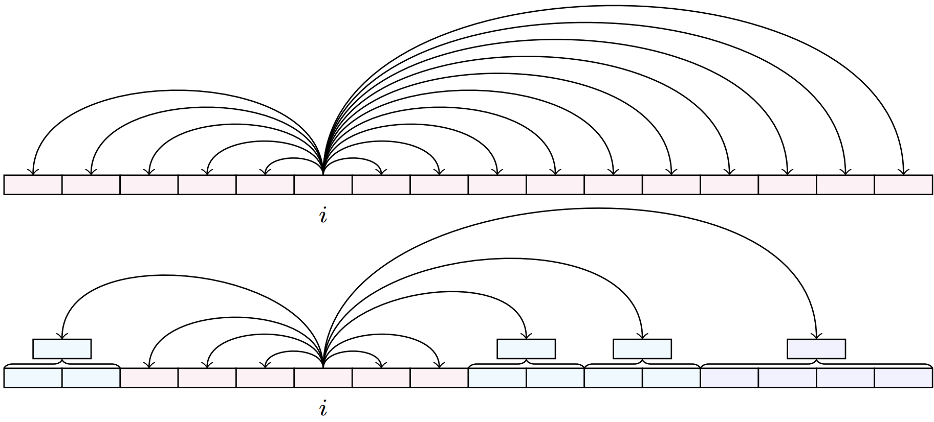
(a) Top: full attention. All pairwise interactions are computed. Bottom: FMA with 3 levels and group size $m=2$. In the neighborhood of a token $i$, attention is computed in full. Tokens far away from $i$ are grouped and downsampled/summarized. The red, green, and purple blocks correspond to the fine level, the first coarse level, and the second coarse level, respectively.

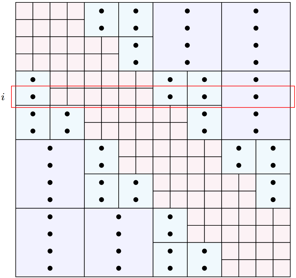
(b) The structure of the FMA attention matrix $\widetilde{C}\approx QK^{\top}$ with 3 levels for group size $m=2$ and approximation rank $p=1$. The highlighted row corresponds to Figure 1(a). Dots represent downsampled query-key products.

Figure 1: Illutration of Fast Multipole Attention (FMA). The influence of the context sequence on token $i$ is computed in a divide-and-conquer way. First, the tokens in the sequence are divided between the immediate neighborhood of $i$ and the rest of the sequence. The influence of the tokens near $i$ (level 0) is computed using full attention. Next, the remaining tokens are divided between the level-1 tokens and the further-away tokens, and the influence of the level-1 tokens is computed using level-1 summarization. This divide-and-conquer strategy is repeated for all subsequent increasingly coarser levels, resulting in an efficient algorithm with complexity $\mathcal{O}(n\log n)$.

Figure 2: Overview of bidirectional FMA with three levels.

Tree Structure To describe our FMA algorithm, we introduce a hierarchical tree structure for dividing the input sequence. We denote the fine-level group size by $m$, which is small compared to $n$. On the fine level, level $0$, tokens are considered individually. Level $1$ contains intervals of size $m_{1}\coloneqq m$. The interval size on the $\ell$-th level is $m_{\ell}\coloneqq 2^{\ell-1}m$ for $\ell=1,\dots,L$, where $L\coloneqq\log_{2}(n/m)-1$. The coarsest level, level $L$, contains intervals of size $n/4$. We assume $n$ is divisible by $m$ and $n/m$ is a power of 2.

Downsampling Keys and Values On level $\ell=1,\dots,L$, FMA downsamples each interval of size $m_{\ell}\times d$ in $K$ and $V$ to $p\times d$, where $p$ is the approximation rank of the off-diagonal blocks and $m$ is divisible by $p$. When $p=1$, each group is summarized by one vector. In our numerical results, we use $p=4$ summary vectors for each block to increase the accuracy of approximation (similar to using multiple heads in attention, or retaining multiple terms in the truncated multipole expansion for the original fast multipole method (Greengard & Rokhlin, 1987; Beatson & Greengard, 1997)). We adopt 1D convolution as the downsampling operator with $\mathtt{kernel\_size=m_{\ell},\,stride=m_{\ell},\,groups=d}$.

For each level, with group size $m_{\ell}$, the 1D convolution learns $p$ convolution kernels of size $m_{\ell}$ for each of the $d$ features. This produces $p$ summarized vectors in each group of size $m_{\ell}$. Therefore, the downsampled key/value matrices, $K^{(\ell)}$ and $V^{(\ell)}$, have size $\dfrac{np}{m_{\ell}}\times d$.

Hierarchical Matrix Structure We introduce a hierarchical structure for an $n\times n$ matrix with the following non-overlapping index sets:

$$I_{0}=\left\{(i,j)\in\left\{0,\dots,n-1\right\}^{2}:\left\lfloor\frac{i}{m}\right\rfloor-\left\lfloor\frac{j}{m}\right\rfloor\in[-1,1]\right\},$$ (3)

$$I_{\ell}=\left\{(i,j)\in\left\{0,\dots,n-1\right\}^{2}:\left\lfloor\frac{i}{m_{\ell}}\right\rfloor-\left\lfloor\frac{j}{m_{\ell}}\right\rfloor\in\{\pm 2,\pm 3\}\right\},\quad\ell=1,...,L.$$ (4)

Here the indices start from 0. The index set $I_{0}$ corresponds to the block tri-diagonals with blocks of size $m$ and the sets $I_{\ell}$ with $\ell\geq 1$ correspond to block super-diagonals and sub-diagonals. Figure 1(b) illustrates the structure of $I_{0}$ (red), $I_{1}$ (green), and $I_{2}$ (purple) for $L=2$ and $m=2$.

Fast Multipole Attention With the hierarchical matrix structure and downsampled keys and values, FMA computes the attention scores at different levels. For a pair $(i,j)\in I_{0}$, the attention score is calculated with the original $Q$ and $K$. For a pair $(i,j)\in I_{\ell}$ with $1\leq\ell\leq L$ , the attention score is calculated on level $\ell$ using $Q$ and $K^{(\ell)}$. Specifically, the attention scores are computed via

$$\widetilde{C}_{i,j}=\begin{cases}Q_{i}K_{j}^{\top}&\quad\left(i,j\right)\in I_{0},\\ Q_{i}\left(K^{(1)}_{\left\lfloor jp/m_{1}\right\rfloor}\right)^{\top}&\quad\left(i,j\right)\in I_{1},\\ \dots\\ Q_{i}\left(K^{(L)}_{\left\lfloor jp/m_{L}\right\rfloor}\right)^{\top}&\quad\left(i,j\right)\in I_{L}.\end{cases}$$ (5)

Here, $Q_{i},K_{j}^{(\ell)}$ denote the $i$th row in $Q$ and the $j$th row in $K^{(\ell)}$, respectively. According to (5), a coarse-level block of size $m_{\ell}\times m_{\ell}$ consists of $p$ unique columns, each repeated for $m_{\ell}/p$ times. Therefore, it can be seen as a rank-$p$ approximation of the corresponding block in the dense attention matrix. $\widetilde{C}$ is a matrix with hierarchical structure as shown in Figure 1(b). In causal attention, the upper triangular part of $\widetilde{C}$ is set to $-\infty$. In practice, the full $n\times n$ matrix $\widetilde{C}$ is not formed. Instead, each unique column in the coarse-level blocks is only calculated and stored once.

To normalize attention scores, $\mathtt{softmax}$ is applied to each row of $\widetilde{C}$,

$$\widetilde{A}_{i,:}=\mathtt{softmax}\left(\widetilde{C}_{i,:}/\sqrt{d}\right),\quad{i=0,\ldots,n-1.}$$ (6)

Next, the attention output on each level is computed by multiplying the normalized attention scores with the values at corresponding locations. Finally, each row of the bidrectional FMA is the sum of outputs from each level:

$$\widetilde{X}_{i}=\underbrace{\sum_{j:(i,j)\in I_{0}}\widetilde{A}_{i,j}V_{j}}_{\text{fine level}}+\underbrace{\sum_{\ell=1}^{L}\sum_{j:(i,j)\in I_{\ell}}\widetilde{A}_{i,j}V^{(\ell)}_{\left\lfloor jp/m_{\ell}\right\rfloor}}_{\text{coarse levels}},\quad{i=0,\ldots,n-1.}$$ (7)

Note that the inner sum in (7) with $m_{\ell}$ terms contains only $p$ different terms (that are each repeated $m_{\ell}/p$ times), and hence this sum is implemented efficiently as a sum of $p$ terms.

3.3 Implementation and Complexity

Implementing (3)-(7) efficiently requires efficient block sparse matrix multiplication and storage, which are not available in standard machine learning frameworks. For faster performance and portability, we build custom CUDA kernels for both forward and backward propagation of FMA with the TVM (Chen et al., 2018b) compiler. Our FMA implementation and the cost of each step are as follows:

1. Calculate $K^{(\ell)}$ and $V^{(\ell)}$ on each level by 1D convolution. This requires $\mathcal{O}(npd\log(n/m))$ time and $\mathcal{O}(npd/m)$ space.

2. Calculate dot-products between queries and keys on level $\ell$ at locations in $I_{\ell}$ as in (5). Then apply $\mathtt{softmax}$ across all levels. In each coarse-level block, each unique column is only computed and stored once. This step requires $\mathcal{O}(mnd+npd\log(n/m))$ time and $\mathcal{O}(mn+np\log(n/m))$ space.

3. Calculate attention output on each level and sum up the attention results on each level as in (7). This requires $\mathcal{O}(mnd+npd\log(n/m))$ time and $\mathcal{O}(nd)$ space.

Figure 2 shows an overview of FMA with three levels. The overall time and space complexity are $\mathcal{O}(mnd+npd\log(n/m))$ and $\mathcal{O}(mn+np\log(n/m))$, where step 2 is dominant.

3.4 Fast Multipole Methods

In this section, we draw connections between the attention mechanism and $n$-body problems and recall the Fast Multipole Method (Greengard & Rokhlin, 1987; Beatson & Greengard, 1997; Martinsson, 2015), which forms the inspiration for Fast Multipole Attention. An $n$-body problem in physics requires evaluating all pairwise influences in a system of $n$ objects, for example, the problem of finding potentials $u_{i}=\sum_{j=1}^{n}g(\bm{x}_{i},\bm{x}_{j})q_{j}$ for $i=1,2,\dots,n$ due to charges $\{q_{i}\}_{i=1}^{n}$ at locations $\{\bm{x}_{i}\}_{i=1}^{n}$, where $g(\cdot,\cdot)$ is the interaction potential of electrostatics. Attention resembles an $n$-body problem if we compare token locations to target/source locations, values to source strengths, and the attention kernel to the interaction kernel.

A popular class of methods to reduce the $\mathcal{O}(n^{2})$ complexity of direct computation in $n$-body problems, the Fast Multipole Method (FMM), partitions the simulation domain into a hierarchy of cells, with each cell containing a small number of particles. It starts from the finest level and computes interactions between points in neighboring cells directly, and moves to coarser levels to compute interactions between distant source-target pairs using compact representations of points in source cells and multipole expansions. In this way, the classic tree code (Barnes & Hut, 1986) reduces the computational complexity of the $n$-body problem from $\mathcal{O}(n^{2})$ to $\mathcal{O}(n\log n)$ with a hierarchical tree structure. The attention matrix of FMA has the same structure as the 1D FMM. FMMformer (Nguyen et al., 2021) approximates self-attention with a near-field and far-field decomposition using 2 levels, combining coarse linearization with local attention.

3.5 H-matrices and H-transformer

The Fast Multipole Method is related to H-matrices (Hackbusch, 1999; Hackbusch & Khoromskij, 2000), which are a class of matrices with block hierarchy and are used in H-transformer (Zhu & Soricut, 2021). In an H-matrix, off-diagonal blocks are replaced by their low-rank approximation. Similar to FMA, the sparsity pattern of the attention matrix in H-transformer is hierarchical and results in linear time and memory complexity, but there are key differences. First, as a crucial advance, we use a learned downsampling method instead of the fixed averaging process used in H-transformer to compute coarse-level average quantities. Second, H-transformer’s fixed averaging requires the approximation rank $p$ to equal the group size $m$, which our experiments show is substantially sub-optimal. Third, unlike the H-matrix structure, in FMA tokens in the immediate left and right neighborhoods are not downsampled and are considered in full resolution, which results in better accuracy. Fourth, our approach has the flexibility to not downsample the queries, which leads to a better balance between accuracy and memory use in practice. Together, these key differences and advances result in FMA being dramatically more accurate than H-transformer, as demonstrated in our language modeling tests.

3.6 Analysis of the Approximation Error

This section discusses the approximation error of the attention matrix of FMA. For convenience, we consider the first query $Q_{0}$ and the case $p=1$. Let $\widetilde{K}\in\mathbb{R}^{n\times d}$ denote the matrix containing the key vectors at different resolutions corresponding to the first query, i.e.,

$$\widetilde{K}=\left[\underbrace{K_{0}^{\top},\dots,K_{2m-1}^{\top}}_{\text{fine level}},\underbrace{K^{(1)\top}_{\left\lfloor\frac{2m}{m_{1}}\right\rfloor},\dots}_{m_{1}\text{ columns}},\underbrace{K^{(1)\top}_{\left\lfloor\frac{3m}{m_{1}}\right\rfloor},\dots}_{m_{1}\text{ columns}},\underbrace{K^{(2)\top}_{\left\lfloor\frac{4m}{m_{2}}\right\rfloor},\dots}_{m_{2}\text{ columns}},\underbrace{K^{(2)\top}_{\left\lfloor\frac{6m}{m_{2}}\right\rfloor},\dots}_{m_{2}\text{ columns}},\dots\right]^{\top},$$ (8)

where each column on coarse levels is repeated for $m_{\ell}$ times. Then $\widetilde{C}_{0}=Q_{0}\widetilde{K}^{\top}.$
Let $\Delta K^{(\ell)}_{j}\coloneqq K_{j}-K^{(\ell)}_{\left\lfloor j/{m_{\ell}}\right\rfloor}$ be the difference between the $j$th key vector and the corresponding downsampled key vector at level $\ell$. Then the approximation error is

$$\left\|C_{0}-\widetilde{C}_{0}\right\|_{1}=\left\|Q_{0}K^{\top}-Q_{0}\widetilde{K}^{\top}\right\|_{1}\leq\left\|Q_{0}\right\|_{1}\left\|K^{\top}-\widetilde{K}^{\top}\right\|_{1}=\left\|Q_{0}\right\|_{1}\max_{\ell,j:(1,j)\in I_{\ell}}\left\|\left(\Delta K^{(\ell)}_{j}\right)^{\top}\right\|_{1},$$ (9)

where $\|\cdot\|_{1}$ denotes the matrix $L_{1}$ norm, i.e., the maximum absolute column sum. Equation (9) implies that the quality of the attention approximation depends on the deviation of the key distribution in each group. Therefore, applying normalization before the self-attention is beneficial to reducing the approximation error.

4 Experiments

In this section, we experimentally analyze the performance of the proposed method. First, we evaluate FMA through autoregressive language modeling on the enwik-8 dataset (Mahoney (2009), Sec. 4.1). Then we evaluate FMA in the bidirectional setting through masked language modeling on Wikitext-103 (Merity et al. (2017), Sec. 4.2). In both tasks, we compare FMA with efficient attention variants used in other works focusing on improving the efficiency of attention for long sequences, including Reformer (Kitaev et al., 2020), Linformer (Wang et al., 2020), Nyströmformer (Xiong et al., 2021), BigBird (Zaheer et al., 2020), and H-transformer (Zhu & Soricut, 2021). The context size varies from 512 to 2K. For fair comparison, we use the same transformer architecture for all attention variants. Finally, in Sec. 4.3, we show a comparative analysis of memory and time cost to demonstrate the ability of FMA to scale efficiently.

We use $p=4$ in our experiments for Fast Multipole Attention and typically use 3, 4 or 5 levels (including the finest level). In general, increasing $m$ and $p$ leads to better accuracy at the cost of larger computational resources (see more detail in the supplementary material). For Linformer, the projection matrices are not shared by queries and keys or shared across layers, and the compression factor is 4. For Reformer, we use two rounds of hashing and the number of buckets is set to the nearest power of two that is greater than or equal to the square root of the input size. We set the numerical rank to be 16 in H-transformer. We conduct the experiments on one NVIDIA Tesla A100 with 80GB of memory and use the $\mathtt{fairseq}$ toolkit (Ott et al., 2019).

4.1 Autoregressive Language Modeling

We consider the enwik-8 dataset, which contains the first $10^{8}$ bytes of the English Wikipedia dump from 2006. We train a character-level autoregressive language model that estimates the distribution of the next token given previous tokens. We adopt the standard transformer decoder with pre-normalization and learned positional embeddings, and replace full attention with other attention variants to compare their performance. The model has 6 layers with embedding dimension 768 and 12 attention heads.

Table 1 shows that with the same context size, FMA obtains lower bpc using less memory than other variants of efficient attention including Reformer, Linformer, Nyströmformer, BigBird, and H-transformer. Also, FMA-linear uses less memory than FMA while achieving comparable bpc. Note that runs that used more than 75 GB of memory were left out from Table 1 (Reformer, Linformer and BigBird with context size 2048). Compared to H-transformer, FMA obtains dramatically better accuracy with smaller memory size.

model	context size	bpc(test)$\downarrow$	memory footprint
Linformer (Wang et al., 2020)	512	1.424	38.2 GB
Nyströmformer Xiong et al. (2021)	512	1.418	14.2 GB
BigBird (Zaheer et al., 2020)	512	1.465	16.4 GB
H-transformer (Zhu & Soricut, 2021)	512	1.853	12.3 GB
FMA-m=64-3lev	512	1.353	11.6 GB
FMA-linear-m=64-3lev	512	1.391	9.8 GB
Reformer (Kitaev et al., 2020)	1024	1.271	31.8 GB
Linformer (Wang et al., 2020)	1024	1.343	74.9 GB
Nyströmformer (Xiong et al., 2021)	1024	1.290	26.9 GB
BigBird (Zaheer et al., 2020)	1024	1.345	23.1 GB
H-transformer (Zhu & Soricut, 2021)	1024	1.789	23.7 GB
FMA-m=64-4lev	1024	1.256	21.6 GB
FMA-linear-m=64-4lev	1024	1.298	17.6 GB
Nyströmformer (Xiong et al., 2021)	2048	1.224	67.1 GB
H-transformer (Zhu & Soricut, 2021)	2048	1.684	38.4 GB
FMA-m=128-4lev	2048	1.220	48.2 GB
FMA-linear-m=128-4lev	2048	1.244	34.1 GB

Table 1: Autoregressive language modeling results on enwik-8. With the same context size, FMA obtains lower bpc using less memory than other variants of efficient attention.

4.2 Bidirectional Language Model

We conduct bidirectional language modeling on Wikitext-103 (Merity et al., 2017), a dataset commonly used for testing long term dependencies in language models, see Table 2. We process Wikitext-103 with Byte Part Encoding tokenization and train a bidirectional language model by randomly masking 15% of the input tokens. We use the Transformer encoder with 6 layers, embedding dimension 768 and 12 attention heads, and we compare the performance and memory cost of different efficient attention variants, including our new FMA, by replacing the full attention module in the Transformer. The results in Table 2 show that our new FMA obtains the best accuracy and lowest memory footprint compared to other efficient transformers from the literature.

model	context size	ppl(test)$\downarrow$	memory footprint
Reformer (Kitaev et al., 2020)	512	11.03	14.6 GB
Linformer (Wang et al., 2020)	512	14.95	11.8 GB
H-transformer (Zhu & Soricut, 2021)	512	10.60	10.7 GB
FMA-m=64-3lev	512	9.45	10.9 GB
FMA-linear-m=64-3lev	512	10.78	8.2 GB
Reformer (Kitaev et al., 2020)	1024	10.56	27.4 GB
Linformer (Wang et al., 2020)	1024	14.24	22.0 GB
H-transformer (Zhu & Soricut, 2021)	1024	9.81	16.9 GB
FMA-m=64-4lev	1024	9.06	18.6 GB
FMA-linear-m=64-4lev	1024	10.13	15.6 GB
Reformer (Kitaev et al., 2020)	2048	9.90	49.2 GB
Linformer (Wang et al., 2020)	2048	14.06	48.1 GB
H-transformer (Zhu & Soricut, 2021)	2048	9.45	33.1 GB
FMA-m=64-5lev	2048	8.95	37.0 GB
FMA-linear-m=64-5lev	2048	9.64	29.5 GB

Table 2: Masked language modeling results on Wikitext-103. With the same context size, our FMA obtains the best accuracy and uses less memory compared to other attention variants.

4.3 Efficiency Comparison

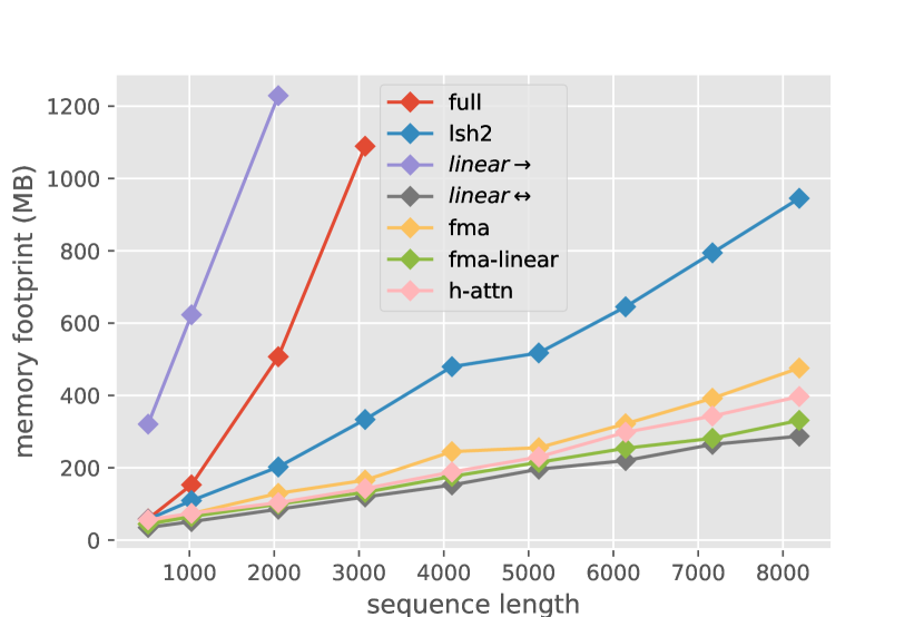
(a) Memory footprint.

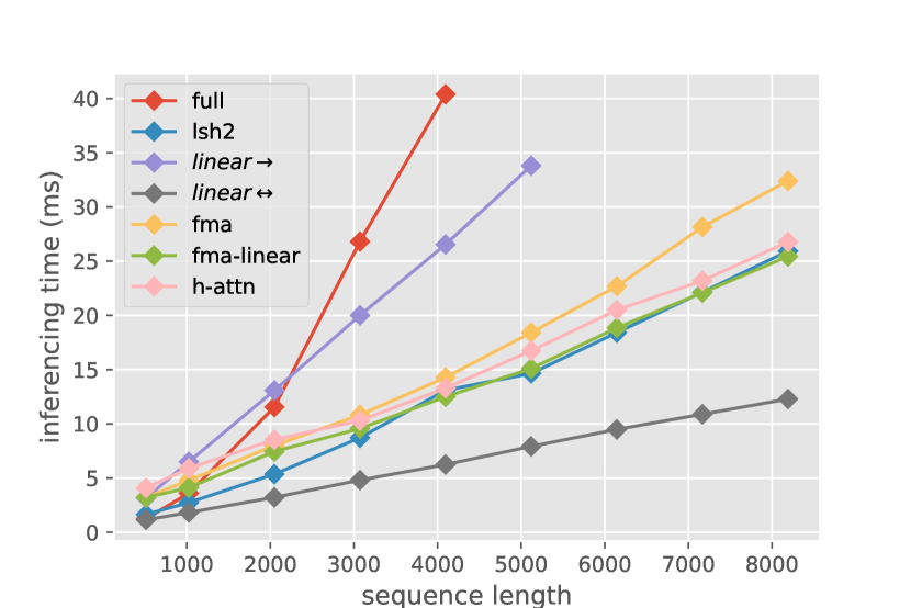
(b) Inferencing time.

Figure 3: Efficiency comparison of attention variants on different input sizes. Here, $\rightarrow$ denotes causal attention, and $\leftrightarrow$ denotes bidirectional attention.

In order to demonstrate the scalability of FMA on long sequences, we compare its inference time and GPU memory footprint to those of full attention, LSH attention, linear attention, and H-attention, which have been used in the original Transformer, Reformer, Linformer, and H-transformer, respectively. The input size varies from 512 to 8K and the batch size, embedding dimension, and number of attention heads are 1, 768, and 12, respectively. We report the performance of full attention, LSH attention, H-attention, and FMA in the causal mode only, as their performance in the bidirectional setting is similar. Linear attention is efficient in the bidirectional setting but expensive in causal mode, and both cases are reported.

As shown in Figure 3, the memory cost of FMA and FMA-linear scales much better than full attention and is lower than or similar to that of other efficient variants. Similarly, the inference speed scales much better than full attention and is similar to that of other efficient variants. However, we should note that our current CUDA kernels are not yet fully optimized and that more efficient implementation of the kernels could further improve the time and memory efficiency.

5 Conclusion

We have presented Fast Multipole Attention, an efficient variant of dot-product attention. With hierarchical grouping and downsampling of queries and keys, FMA achieves $\mathcal{O}(n\log n)$ or $\mathcal{O}(n)$ complexity while retaining a global receptive field. In both autoregressive and bidirectional tasks,
our FMA outperforms three other efficient attention variants overall. FMA is versatile and robust as it can be used as a drop-in replacement of causal or bidirectional attention without changing the model architecture or the training schedule. The high efficiency of FMA has the potential to empower large language models with much greater sequence lengths, taking the full context into account in a naturally hierarchical manner during training and when generating long sequences. As for the Fast Multipole Method, the algorithmic principle of Fast Multipole Attention can naturally be extended to arrays in multiple dimensions including images and videos, so our new Fast Multipole Attention approach promises to have wide applications beyond language modeling.

Appendix A Supplementary Material

A.1 FMA-linear

FMA-linear is described as follow. First, queries, keys, and values are downsampled to get $Q^{(\ell)}$, $K^{(\ell)}$, and $V^{(\ell)}$ for $\ell=1,\dots,L$. The attention scores are computed by

$$\widetilde{C}_{i,j}=\begin{cases}Q_{i}K_{j}^{\top}&\quad\left(i,j\right)\in I_{0},\\ \left(Q^{(1)}_{\left\lfloor ip/m_{1}\right\rfloor}\right)\left(K^{(1)}_{\left\lfloor jp/m_{1}\right\rfloor}\right)^{\top}&\quad\left(i,j\right)\in I_{1},\\ \dots\\ \left(Q^{(L)}_{\left\lfloor ip/m_{L}\right\rfloor}\right)\left(K^{(L)}_{\left\lfloor jp/m_{L}\right\rfloor}\right)^{\top}&\quad\left(i,j\right)\in I_{L}.\end{cases}$$ (10)

For $\ell=0,\dots,L$ and each entry $\left(i,j\right)\in I_{\ell}$, softmax is computed at each level:

$$\widetilde{A}_{i,j}=\frac{\exp\left(\widetilde{C}_{i,j}/\sqrt{d}\right)}{\sum_{\left(i,k\right)\in I_{\ell}}\exp\left(\widetilde{C}_{i,k}/\sqrt{d}\right)}.$$ (11)

Finally, the output is given by

$$\widetilde{X}_{i}=\sum_{j:(i,j)\in I_{0}}\widetilde{A}_{i,j}V_{j}+\sum_{\ell=1}^{L}\sum_{j:(i,j)\in I_{\ell}}\widetilde{A}_{i,j}V^{(\ell)}_{\left\lfloor jp/m_{\ell}\right\rfloor},\quad{i=0,\ldots,n-1.}$$ (12)

A.2 Different Settings of the fine level size $m$ and and the rank $p$

To explore the effect of changing the fine level size $m$ and and the rank $p$ in FMA, we conduct experiments on enwik-8 and measure the bpc and the memory cost. Table 3 shows that increasing $m$ and $p$ gives lower bpc at the cost of an increased memory footprint. Similar to Section 4.1, the model has 6 layers with embedding dimension 768 and 12 attention heads. The memory cost for storing the attention matrix with hierarchical structure is $\mathcal{O}(mn+np\log(n/m))$, which is the dominant part of the total memory footprint for large sequence lengths. In the main paper we consistently use $p=4$, which gives a good balance between accuracy and memory use.

model	bpc(test)	memory footprint
FMA-m32-p2	1.272	19.3 GB
FMA-m32-p4	1.266	19.7 GB
FMA-m32-p8	1.262	21.1 GB
FMA-m64-p2	1.258	20.9 GB
FMA-m64-p4	1.256	21.6 GB
FMA-m64-p8	1.251	23.2 GB

Table 3: Autoregressive language modeling results with different $m$ and $p$ on enwik-8 with context size 1024.

A.3 TVM tensor expressions

We implement FMA using TVM in four stages. This section contains the mathematical expressions used by the TVM compilers:

1. Local outgoing expansion, which calculates the attention locally on the fine level.

2. Far-field outgoing expansion, which calculates the attention at far away locations on coarse levels.

3. Local incoming expansion, which gathers the values from the neighborhood on the fine level.

4. Far-field incoming expansion, which gathers the values from far away locations on coarse levels.

For simplicity, we denote $\frac{\partial\mathcal{L}}{\partial M_{ij}}$ by $\partial M(i,j)$ for a scalar $\mathcal{L}$ and matrix $M$.

A.3.1 Local outgoing expansion

Forward: For $Q\in\mathbb{R}^{n\times d},K\in\mathbb{R}^{n\times d}$, the output matrix $Z\in\mathbb{R}^{n\times 2m}$ is given by

$$Z(i,j)=\sum_{k=0}^{d-1}Q(i,k)K(m\lfloor i/m\rfloor+j,k).$$ (13)

Backward: For $\partial Z\in\mathbb{R}^{n\times 2m},K\in\mathbb{R}^{n\times d}$, the partial gradient $\partial Q\in\mathbb{R}^{n\times d}$ is given by

$$\partial Q(i,j)=\sum_{k=0}^{2m-1}\partial Z(i,k)K(m\lfloor i/m\rfloor+k,j).$$ (14)

For $\partial Z\in\mathbb{R}^{n\times 2m},Q\in\mathbb{R}^{n\times d}$, the partial gradient $\partial K\in\mathbb{R}^{n\times d}$ is given by

$$\partial K(i,j)=\sum_{k=0}^{m-1}\partial Z(m\lfloor i/m\rfloor+k,i\%m+m)Q(m\lfloor i/m\rfloor+k,j)$$

$$+\sum_{k=m}^{2m-1}\partial Z(m\lfloor i/m\rfloor+k,i\%m)Q(m\lfloor i/m\rfloor+k,j).$$ (15)

A.3.2 Far-field outgoing expansion

Forward: For $Q\in\mathbb{R}^{n\times d},K\in\mathbb{R}^{n_{\ell}\times d}$, the output matrix $Z\in\mathbb{R}^{n\times 2p}$ is given by

$$Z(i,j)=\sum_{k=0}^{d-1}Q(i,k)K(2p\lfloor i/2w\rfloor+j,k),$$ (16)

with $w\coloneqq p\frac{n}{n_{l}}$.

Backward: For $\partial Z\in\mathbb{R}^{n\times 2p},K\in\mathbb{R}^{n_{\ell}\times d}$, the partial gradient $\partial Q\in\mathbb{R}^{n\times d}$ is given by

$$\partial Q(i,j)=\sum_{k=0}^{2p-1}\partial Z(i,k)K(2p\lfloor i/2w\rfloor+k,j).$$ (17)

For $\partial Z\in\mathbb{R}^{n\times 2p},Q\in\mathbb{R}^{n\times d}$, the partial gradient $\partial K\in\mathbb{R}^{n_{\ell}\times d}$ is given by

$$\partial K(i,j)=\sum_{k=0}^{2w-1}\partial Z(2w(\lfloor i/2p\rfloor+1)+k,i\%2p)Q(2w(\lfloor i/2p\rfloor+1)+k,j).$$ (18)

A.3.3 Local incoming expansion

Forward: For $C\in\mathbb{R}^{n\times 2m},V\in\mathbb{R}^{n\times d}$, the output matrix $Z\in\mathbb{R}^{n\times d}$ is given by

$$Z(i,j)=\sum_{k=0}^{2m-1}C(i,k)V(m\lfloor i/m\rfloor+k,j).$$ (19)

Backward: For $\partial Z\in\mathbb{R}^{n\times d},V\in\mathbb{R}^{n\times d}$, the partial gradient $\partial C\in\mathbb{R}^{n\times 2m}$ is given by

$$\partial C(i,j)=\sum_{k=0}^{d-1}\partial Z(i,k)V(m\lfloor i/m\rfloor+j,k).$$ (20)

For $\partial Z\in\mathbb{R}^{n\times d},C\in\mathbb{R}^{n\times 2m}$, the partial gradient $\partial V\in\mathbb{R}^{n\times d}$ is given by

$$\partial V(i,j)=\sum_{k=0}^{m-1}\partial Z(m\lfloor i/m\rfloor+k,j)C(m\lfloor i/m\rfloor+k,i\%m+m)$$

$$+\sum_{k=m}^{2m-1}\partial Z(m\lfloor i/m\rfloor+k,j)C(m\lfloor i/m\rfloor+k,i\%m).$$ (21)

A.3.4 Far-field incoming expansion

Forward: For $C\in\mathbb{R}^{n\times 2p},V\in\mathbb{R}^{n_{\ell}\times d}$, the output matrix $Z\in\mathbb{R}^{n\times d}$ is given by

$$Z(i,j)=\sum_{k=0}^{2p-1}C(i,k)V(2p\lfloor i/2w\rfloor+k,j).$$ (22)

Backward: For $\partial Z\in\mathbb{R}^{n\times d},V\in\mathbb{R}^{n_{\ell}\times d}$, the partial gradient $\partial C\in\mathbb{R}^{n\times 2p}$ is given by

$$\partial C(i,j)=\sum_{k=0}^{d-1}\partial Z(i,k)V(2p\lfloor i/2w\rfloor+j,k).$$ (23)

For $\partial Z\in\mathbb{R}^{n\times d},C\in\mathbb{R}^{n\times 2p}$, the partial gradient $\partial V\in\mathbb{R}^{n_{\ell}\times d}$ is given by

$$\partial V(i,j)=\sum_{k=0}^{2w-1}\partial Z(2w(\lfloor i/2p\rfloor+1)+k,j)C(2w(\lfloor i/2p\rfloor+1)+k,i\%2p).$$ (24)

References

- Ainslie et al. (2020) Joshua Ainslie, Santiago Ontanon, Chris Alberti, Vaclav Cvicek, Zachary Fisher, Philip Pham, Anirudh Ravula, Sumit Sanghai, Qifan Wang, and Li Yang. ETC: Encoding long and structured inputs in transformers. In Proceedings of the 2020 Conference on Empirical Methods in Natural Language Processing (EMNLP), pp. 268–284, 2020.
- Bahdanau et al. (2014) Dzmitry Bahdanau, Kyunghyun Cho, and Yoshua Bengio. Neural machine translation by jointly learning to align and translate, 2014.
- Barnes & Hut (1986) Josh Barnes and Piet Hut. A hierarchical O(N log N) force-calculation algorithm. Nature, 324(6096):446–449, December 1986.
- Beatson & Greengard (1997) Rick Beatson and Leslie Greengard. A short course on fast multipole methods. Wavelets, multilevel methods and elliptic PDEs, 1:1–37, 1997.
- Beltagy et al. (2020) Iz Beltagy, Matthew E. Peters, and Arman Cohan. Longformer: The long-document transformer. arXiv:2004.05150, 2020.
- Brown et al. (2020) Tom B. Brown, Benjamin Mann, Nick Ryder, Melanie Subbiah, Jared Kaplan, Prafulla Dhariwal, Arvind Neelakantan, Pranav Shyam, Girish Sastry, Amanda Askell, Sandhini Agarwal, Ariel Herbert-Voss, Gretchen Krueger, Tom Henighan, Rewon Child, Aditya Ramesh, Daniel M. Ziegler, Jeffrey Wu, Clemens Winter, Christopher Hesse, Mark Chen, Eric Sigler, Mateusz Litwin, Scott Gray, Benjamin Chess, Jack Clark, Christopher Berner, Sam McCandlish, Alec Radford, Ilya Sutskever, and Dario Amodei. Language models are few-shot learners, 2020.
- Chamberlain et al. (2021) Benjamin Paul Chamberlain, James Rowbottom, Maria I. Gorinova, Stefan D Webb, Emanuele Rossi, and Michael M. Bronstein. GRAND: Graph neural diffusion. In The Symbiosis of Deep Learning and Differential Equations, 2021.
- Chen et al. (2018a) Ricky TQ Chen, Yulia Rubanova, Jesse Bettencourt, and David K Duvenaud. Neural ordinary differential equations. Advances in neural information processing systems, 31, 2018a.
- Chen et al. (2018b) Tianqi Chen, Thierry Moreau, Ziheng Jiang, Lianmin Zheng, Eddie Yan, Meghan Cowan, Haichen Shen, Leyuan Wang, Yuwei Hu, Luis Ceze, Carlos Guestrin, and Arvind Krishnamurthy. TVM: An automated end-to-end optimizing compiler for deep learning. In Proceedings of the 13th USENIX Conference on Operating Systems Design and Implementation, pp. 579–594, 2018b.
- Child et al. (2019) Rewon Child, Scott Gray, Alec Radford, and Ilya Sutskever. Generating long sequences with sparse transformers, 2019.
- Choromanski et al. (2021) Krzysztof Marcin Choromanski, Valerii Likhosherstov, David Dohan, Xingyou Song, Andreea Gane, Tamas Sarlos, Peter Hawkins, Jared Quincy Davis, Afroz Mohiuddin, Lukasz Kaiser, David Benjamin Belanger, Lucy J Colwell, and Adrian Weller. Rethinking attention with Performers. In International Conference on Learning Representations, 2021.
- Devlin et al. (2019) Jacob Devlin, Ming-Wei Chang, Kenton Lee, and Kristina Toutanova. BERT: Pre-training of deep bidirectional transformers for language understanding. In Proceedings of the 2019 Conference of the North American Chapter of the Association for Computational Linguistics: Human Language Technologies, Volume 1 (Long and Short Papers), pp. 4171–4186, 2019.
- Dosovitskiy et al. (2021) Alexey Dosovitskiy, Lucas Beyer, Alexander Kolesnikov, Dirk Weissenborn, Xiaohua Zhai, Thomas Unterthiner, Mostafa Dehghani, Matthias Minderer, Georg Heigold, Sylvain Gelly, Jakob Uszkoreit, and Neil Houlsby. An image is worth 16x16 words: Transformers for image recognition at scale. In International Conference on Learning Representations, 2021.
- Eliasof et al. (2021) Moshe Eliasof, Eldad Haber, and Eran Treister. PDE-GCN: novel architectures for graph neural networks motivated by partial differential equations. Advances in neural information processing systems, 34:3836–3849, 2021.
- Greengard & Rokhlin (1987) Leslie Greengard and Vladimir Rokhlin. A fast algorithm for particle simulations. Journal of computational physics, 73(2):325–348, 1987.
- Gulati et al. (2020) Anmol Gulati, James Qin, Chung-Cheng Chiu, Niki Parmar, Yu Zhang, Jiahui Yu, Wei Han, Shibo Wang, Zhengdong Zhang, Yonghui Wu, and Ruoming Pang. Conformer: Convolution-augmented Transformer for Speech Recognition. In Proc. Interspeech 2020, pp. 5036–5040, 2020.
- Günther et al. (2020) Stefanie Günther, Lars Ruthotto, Jacob B. Schroder, Eric C. Cyr, and Nicolas R. Gauger. Layer-parallel training of deep residual neural networks. SIAM Journal on Mathematics of Data Science, 2(1):1–23, 2020.
- Haber & Ruthotto (2017) Eldad Haber and Lars Ruthotto. Stable architectures for deep neural networks. Inverse problems, 34(1):014004, 2017.
- Hackbusch (1999) W. Hackbusch. A Sparse Matrix Arithmetic Based on H-Matrices. Part I: Introduction to H-Matrices. Computing, 62(2):89–108, 1999.
- Hackbusch & Khoromskij (2000) Wolfgang Hackbusch and B. Khoromskij. A Sparse H-Matrix Arithmetic, Part II: Application to Multi-Dimensional Problems. Computing, 64, January 2000.
- Huang et al. (2019) Cheng-Zhi Anna Huang, Ashish Vaswani, Jakob Uszkoreit, Ian Simon, Curtis Hawthorne, Noam Shazeer, Andrew M. Dai, Matthew D. Hoffman, Monica Dinculescu, and Douglas Eck. Music transformer. In International Conference on Learning Representations, 2019.
- Jumper et al. (2021) John Jumper, Richard Evans, Alexander Pritzel, Tim Green, Michael Figurnov, Olaf Ronneberger, Kathryn Tunyasuvunakool, Russ Bates, Augustin Žídek, Anna Potapenko, et al. Highly accurate protein structure prediction with alphafold. Nature, 596(7873):583–589, 2021.
- Katharopoulos et al. (2020) Angelos Katharopoulos, Apoorv Vyas, Nikolaos Pappas, and François Fleuret. Transformers are RNNs: Fast autoregressive transformers with linear attention. In Proceedings of the 37th International Conference on Machine Learning, volume 119, pp. 5156–5165, 2020.
- Kitaev et al. (2020) Nikita Kitaev, Lukasz Kaiser, and Anselm Levskaya. Reformer: The efficient transformer. In International Conference on Learning Representations, 2020.
- Li et al. (2021) Zongyi Li, Nikola Borislavov Kovachki, Kamyar Azizzadenesheli, Burigede liu, Kaushik Bhattacharya, Andrew Stuart, and Anima Anandkumar. Fourier neural operator for parametric partial differential equations. In International Conference on Learning Representations, 2021.
- Liu et al. (2018) Peter J. Liu, Mohammad Saleh, Etienne Pot, Ben Goodrich, Ryan Sepassi, Lukasz Kaiser, and Noam Shazeer. Generating wikipedia by summarizing long sequences, 2018.
- Mahoney (2009) Matt Mahoney. Large text compression benchmark, 2009.
- Martinsson (2015) Per-Gunnar Martinsson. Fast Multipole Methods, pp. 498–508. 2015.
- Maruf et al. (2021) Sameen Maruf, Fahimeh Saleh, and Gholamreza Haffari. A survey on document-level neural machine translation: Methods and evaluation. ACM Computing Surveys (CSUR), 54(2):1–36, 2021.
- Merity et al. (2017) Stephen Merity, Caiming Xiong, James Bradbury, and Richard Socher. Pointer sentinel mixture models. In International Conference on Learning Representations, 2017.
- Nguyen et al. (2021) Tan Nguyen, Vai Suliafu, Stanley Osher, Long Chen, and Bao Wang. FMMformer: efficient and flexible transformer via decomposed near-field and far-field attention. Advances in neural information processing systems, 34:29449–29463, 2021.
- Ott et al. (2019) Myle Ott, Sergey Edunov, Alexei Baevski, Angela Fan, Sam Gross, Nathan Ng, David Grangier, and Michael Auli. fairseq: A fast, extensible toolkit for sequence modeling. In Proceedings of the 2019 Conference of the North American Chapter of the Association for Computational Linguistics (Demonstrations), pp. 48–53, 2019.
- Peng et al. (2021) Hao Peng, Nikolaos Pappas, Dani Yogatama, Roy Schwartz, Noah Smith, and Lingpeng Kong. Random feature attention. In International Conference on Learning Representations, 2021.
- Qin et al. (2022) Zhen Qin, Weixuan Sun, Hui Deng, Dongxu Li, Yunshen Wei, Baohong Lv, Junjie Yan, Lingpeng Kong, and Yiran Zhong. cosFormer: Rethinking softmax in attention. In International Conference on Learning Representations, 2022.
- Roy et al. (2021) Aurko Roy, Mohammad Saffar, Ashish Vaswani, and David Grangier. Efficient content-based sparse attention with routing transformers. Transactions of the Association for Computational Linguistics, 9:53–68, 2021.
- Tay et al. (2022) Yi Tay, Mostafa Dehghani, Dara Bahri, and Donald Metzler. Efficient transformers: A survey. ACM Comput. Surv., 55(6), 2022.
- Vaswani et al. (2017) Ashish Vaswani, Noam Shazeer, Niki Parmar, Jakob Uszkoreit, Llion Jones, Aidan N Gomez, Łukasz Kaiser, and Illia Polosukhin. Attention is all you need. Advances in neural information processing systems, 30, 2017.
- Vyas et al. (2020) Apoorv Vyas, Angelos Katharopoulos, and François Fleuret. Fast transformers with clustered attention. In Proceedings of the 34th International Conference on Neural Information Processing Systems, 2020.
- Wang et al. (2022) Ningning Wang, Guobing Gan, Peng Zhang, Shuai Zhang, Junqiu Wei, Qun Liu, and Xin Jiang. ClusterFormer: Neural clustering attention for efficient and effective transformer. In Proceedings of the 60th Annual Meeting of the Association for Computational Linguistics (Volume 1: Long Papers), pp. 2390–2402, 2022.
- Wang et al. (2021) Shuohang Wang, Luowei Zhou, Zhe Gan, Yen-Chun Chen, Yuwei Fang, Siqi Sun, Yu Cheng, and Jingjing Liu. Cluster-former: Clustering-based sparse transformer for question answering. In Findings of the Association for Computational Linguistics: ACL-IJCNLP 2021, pp. 3958–3968, 2021.
- Wang et al. (2020) Sinong Wang, Belinda Z Li, Madian Khabsa, Han Fang, and Hao Ma. Linformer: Self-attention with linear complexity. arXiv preprint arXiv:2006.04768, 2020.
- Xiong et al. (2021) Yunyang Xiong, Zhanpeng Zeng, Rudrasis Chakraborty, Mingxing Tan, Glenn Fung, Yin Li, and Vikas Singh. Nyströmformer: A nyström-based algorithm for approximating self-attention. In AAAI, pp. 14138–14148, 2021.
- Zaheer et al. (2020) Manzil Zaheer, Guru Guruganesh, Kumar Avinava Dubey, Joshua Ainslie, Chris Alberti, Santiago Ontanon, Philip Pham, Anirudh Ravula, Qifan Wang, Li Yang, and Amr Ahmed. Big Bird: Transformers for longer sequences. In Advances in Neural Information Processing Systems, volume 33, pp. 17283–17297, 2020.
- Zhu & Soricut (2021) Zhenhai Zhu and Radu Soricut. H-Transformer-1D: Fast One-Dimensional Hierarchical Attention for Sequences. In Proceedings of the 59th Annual Meeting of the Association for Computational Linguistics and the 11th International Joint Conference on Natural Language Processing (Volume 1: Long Papers), pp. 3801–3815, 2021.