A Multi-Scale Decomposition MLP-Mixer for
Time Series Analysis

Abstract

Time series data, often characterized by unique composition and complex multi-scale temporal variations, requires special consideration of decomposition and multi-scale modeling in its analysis. Existing deep learning methods on this best fit to only univariate time series, and have not sufficiently accounted for sub-series level modeling and decomposition completeness. To address this, we propose MSD-Mixer, a Multi-Scale Decomposition MLP-Mixer which learns to explicitly decompose the input time series into different components, and represents the components in different layers. To handle multi-scale temporal patterns and inter-channel dependencies, we propose a novel temporal patching approach to model the time series as multi-scale sub-series, i.e., patches, and employ MLPs to mix intra- and inter-patch variations and channel-wise correlations. In addition, we propose a loss function to constrain both the magnitude and autocorrelation of the decomposition residual for decomposition completeness. Through extensive experiments on various real-world datasets for five common time series analysis tasks (long- and short-term forecasting, imputation, anomaly detection, and classification), we demonstrate that MSD-Mixer consistently achieves significantly better performance in comparison with other state-of-the-art task-general and task-specific approaches.

I Introduction

A time series is a sequence of data points indexed in time order. It typically consists of successive numerical observations obtained in a fixed time interval. In multivariate time series each observation contains more than one variable which forms the channel dimension. With the fast development of sensing and data storage technologies, time series data is now becoming omnipresent in our lives, from weather conditions and urban traffic flow to personal health data monitored by smart wearable devices. The analysis of time series data, such as forecasting [1], missing data imputation [2], anomaly detection [3, 4], and classification [5], is therefore facilitating more and more real-world applications, and attracts increasing research interest from both the academia and the industry.

In contrast to images and natural languages, time series data is characterized by its special composition and complex temporal patterns or correlations. Specifically, each data point in a time series is actually a superposition of various underlying temporal patterns plus noise at that time. To better model and analyze it, it is hence important to decompose the time series into disentangled components corresponding to different temporal patterns [6, 7]. Furthermore, time series data carries the semantic information of the temporal patterns in local consecutive data points termed sub-series, instead of in individual data point [8, 9, 10, 11]. The temporal patterns may also be in multiple timescales, hence making it important to extract sub-sereis features and model their change in multiple time scales. To make the problem even more complex, multivariate time series may involve intricate correlations between different channels [12, 13]. These characteristics all make time series analysis a challenging problem.

Recent approaches for time series analysis take advantage of the strong expressiveness of deep learning, and have achieved significant performance in various tasks. However, most efforts are based on deep learning architectures originally designed for image and natural language data, e.g., the Transformer [14]. They either have not considered the decomposition of temporal patterns, or employed only simple decomposition on trend and seasonal components [15, 16], which makes it hard for them to handle multiple intricate temporal patterns in time series data [17, 18]. Considering the special composition of time series, some methods adopt a deep learning architecture that decomposes components from the input for forecasting [19, 20, 21].

However, without considering inter-channel dependency, [19, 20] are best applicable to univariate rather than multivariate time series. Also, they either base on plain MLP on the temporal dimension, or the Transformer [21], which do not take into account the sub-series level features. All the aforementioned works have not considered the residual of the decomposition, which may lead to incomplete decomposition, i.e., meaningful temporal patterns may be left in the residual and not utilized.

In this work, we propose MSD-Mixer, a novel Multi-Scale Decomposition MLP-Mixer to analyze both univariate and multivariate time series. MSD-Mixer learns to explicitly decompose the input time series into different components by generating the component representations in different layers, and accomplishes the analysis task based on such representations. In MSD-Mixer we propose a novel multi-scale temporal patching approach. It divides the input time series into non-overlapping patches along the temporal dimension in each layer, and treats the time series as patches. Different layers have different patch sizes such that they can focus on different time scales. To better model multi-scale temporal patterns and inter-channel dependencies, MSD-Mixer employs multi-layer perceptrons (MLPs) along different dimensions to mix intra- and inter-patch variations and channel-wise correlations. For the completeness of the decomposition, we propose a novel loss function for MSD-Mixer to constrain both the magnitude and autocorrelation of the decomposition residual. Used together with the loss from the target analysis task during training, the loss function helps MSD-Mixer to extract more temporal patterns into the components to be utilized for the target task.

Empowered by the above decomposition and multi-scale modeling, MSD-Mixer distinguishes itself as a task-general backbone that can be trained to accomplish various time series analysis tasks. Through extensive experiments on various real-world datasets, we demonstrate that MSD-Mixer consistently outperforms the state-of-the-art task-general and task-specific approaches by a wide margin on five common tasks, namely long-term forecasting (up to 9.8% in MSE), short-term forecasting (up to 5.6% in OWA), imputation (up to 46.1% in MSE), anomaly detection (up to 33.1% in F1-score) and classification (up to 6.5% in accuracy).

To summarize, we make the following contributions in this paper:

• A novel task-general backbone MSD-Mixer that is well designed to analyze both univariate and multivariate time series, by explicitly decomposing the time series into different components.

• A multi-scale temporal patching approach in MSD-Mixer with MLPs to model the time series data as multi-scale sub-series level patches, which learns accurately the multi-scale temporal patterns in the data.

• A Residual Loss for MSD-Mixer to constrain both the magnitude and autocorrelation of the decomposition residual to achieve decomposition completeness.

• Extensive experiments on 26 datasets for five common time series analysis tasks to validate the effectiveness of MSD-Mixer.

The remainder of this paper is organized as follows: We first review related works in Section II, followed by detailed introduction of MSD-Mixer and its components in Section III. We show the experimental results in Section IV, and conclude in Section V.

II Related Works

As one of the fundamental data modalities, time series has been well studied for long in various science and engineering domains which rely on temporal measurements, and has been most discussed for forecasting [7]. Regarding the special composition and the complex temporal patterns of time series data, early approaches employ manually designed rules or function models to decompose the time series data, such that the temporal patterns can be disentangled and modeled separately [22, 23, 24, 25, 26, 27, 28]. The decomposition usually consists of several components representing different temporal patterns, plus a residual which is constrained to be noise with no meaningful information. However, these approaches usually require considerable domain knowledge and manual effort to be applied for specific domain applications, and are less expressive and scalable considering nowadays large multivariate time series datasets with complex temporal patterns and channel-wise correlations.

In recent years, deep learning has been widely applied in time series analysis for its strong expressiveness and scalability on large and complex datasets. The deep learning based approaches either apply MLP [29], convolutional neural network (CNN) [30, 31, 32, 8], recurrent neural network (RNN) [33], Transformer [5, 9, 4], or their combination [34, 10] to model the time series data for specific tasks. Specifically, Transformer-based models are taking the lead in many time series analysis tasks due to the powerful capability of attention mechanism to capture long-sequence dependencies. Many works has been done to further improve the efficiency [35, 36] and effectiveness [15, 16, 37] of Transformers for time series data. However, it is recently pointed out that the attention mechanism, which relies on point-wise correlations, is not the best solution for time series data, since the semantic information is embedded in the sub-series level variations [11]. In light of this, latest time series forecasting schemes try to combine patch modeling with Transformer and CNN for better forecasting performance [8, 9].

However, despite the above-mentioned achievements, most deep learning based approaches do not consider the decomposition of temporal patterns, or only consider the simple decomposition of very limited type and number of components [15, 16], which makes it hard for them to deal with multiple intricate temporal patterns in time series data [18]. By combining deep learning with decomposition, some schemes show promising results in univariate [19, 20] and multivariate [21] time series forecasting. While impressive, [19, 20] do not consider the inter-channel correlation, which has been shown critical in multivariate time series analysis tasks. Meanwhile, [19, 20] are based on plain MLP on the temporal dimension, and [21] are based on point-wise self-attention for temporal pattern modeling, which do not take into account the sub-series level features. Moreover, all of them simply ignore the residual of the decomposition, which may lead to incomplete decomposition that meaningful temporal patterns can be left in the residual and not utilized. In comparison, we propose MSD-Mixer that advances [19] and [20] with multi-scale temporal patching and multi-dimensional MLP mixing for multi-scale sub-series and inter-channel modeling. Meanwhile, we propose a residual loss to guarantee the completeness of the decomposition process in MSD-Mixer. Furthermore, we experiment MSD-Mixer on various datasets and tasks to show its superior performance.

III MSD-Mixer

In this section, we first formally introduce the definition of general time series analysis problems and time series decomposition in III-A. Then, we overview the architecture and workflow of our proposed MSD-Mixer in Section III-B, followed by elaboration of the key designs in MSD-Mixer in Sections III-C to III-E

III-A Problem Settings

In this work, we consider the general learning based time series analysis problem: Given a dataset $\mathcal{D}$ containing sample pairs $(\boldsymbol{X},\boldsymbol{Y})$, where $\boldsymbol{X}\in\mathbb{R}^{C\times L}$ denotes the input multivariate time series with $C$ channels and $L$ time steps, and $\boldsymbol{Y}$ denotes the label, which is subject to specific time series analysis tasks. For example, $\boldsymbol{Y}\in\mathbb{R}^{C\times H}$ in a forecasting task with horizon size $H$, and $\boldsymbol{Y}\in\mathbb{R}^{M}$ in a classification task with $M$ target classes. The time series analysis problem is to learn a target function $\mathcal{F}(\cdot)$ on the dataset that maps the input $\boldsymbol{X}$ to its corresponding label as $\boldsymbol{\hat{Y}}=\mathcal{F}(\boldsymbol{X})$. Different time series analysis task generally use different task-specific loss functions $\mathcal{L}_{t}(\boldsymbol{Y},\boldsymbol{\hat{Y}})$ to train the model, e.g., cross entropy loss used in classification and mean square error loss used in forecasting.

As $\boldsymbol{X}$ can involve various underlying temporal patterns and noise, we consider decomposing $\boldsymbol{X}$ into $k$ components:

$$\boldsymbol{X}=\sum_{i=1}^{k}\boldsymbol{S}_{i}+\boldsymbol{R},$$ (1)

where $\boldsymbol{S}_{i},\boldsymbol{R}\in\mathbb{R}^{C\times L}$ denote the $i$-th component ($i=1,...,k$) and the residual, respectively. Furthermore, suppose each component $\boldsymbol{S}_{i}$ has a lower-dimensional representation $\boldsymbol{E}_{i}$ that $\boldsymbol{S}_{i}=h_{i}(\boldsymbol{E}_{i})$, where $h_{i}(\cdot)$ denotes the map function for the $i$-th component, then the target $\mathcal{F}$ can be divided and conquered by a series of functions $f_{i}(\cdot)$ of the representations of the components:

$$\boldsymbol{Y}=\mathcal{F}(\boldsymbol{X})=\sum_{i=1}^{k}f_{i}(\boldsymbol{E}_{i}).$$ (2)

III-B MSD-Mixer Overview

Figure 1 shows the overall architecture of MSD-Mixer. MSD-Mixer comprises a stack of $k$ layers, and learns to hierarchically decompose the input $\boldsymbol{X}$ into $k$ components $\{\boldsymbol{S}_{1},...,\boldsymbol{S}_{k}\}$ by generating their lower-dimensional representations $\{\boldsymbol{E}_{1},...,\boldsymbol{E}_{k}\}$ in the corresponding layers. The number of layers and components $k$ is a hyperparameter in MSD-Mixer which should be determined according to the properties of the dataset. Here we define $\boldsymbol{Z}_{0}=\boldsymbol{X}$, and

$$\boldsymbol{Z}_{i}=\boldsymbol{X}-\sum_{j=1}^{k}\boldsymbol{S}_{j},(l=1,...,k),$$ (3)

such that $\boldsymbol{Z}_{i}$ specifies the remaining part after the first $i$ components has been decomposed from the input $\boldsymbol{X}$, and we have

$$\boldsymbol{Z}_{i}=\boldsymbol{Z}_{i-1}-\boldsymbol{S}_{i}.$$ (4)

Following Equation 4, the $i$-th layer of MSD-Mixer takes $\boldsymbol{Z}_{i-1}$ as input, and learns to generate $\boldsymbol{S}_{i}$ from $\boldsymbol{Z}_{i-1}$. As is shown in Figure 1, $\boldsymbol{Z}_{i-1}$ is first patched in the Patching module, and then fed into the MLP-Mixer based Patch Encoder module to generate the representation of $i$-th components as $\boldsymbol{E}_{i}=g_{i}(\boldsymbol{Z}_{i-1})$. The MLP-Mixer based Patch Decoder module then reconstruct $\boldsymbol{S}_{i}$ from $\boldsymbol{E}_{i}$, and the Unpatching module unpatch it to the original dimensionality. After that, $\boldsymbol{S}_{i}$ is subtracted from $\boldsymbol{Z}_{i-1}$ to obtain $\boldsymbol{Z}_{i}$. $\boldsymbol{Z}_{i}$ is fed to the next layer as input for further decomposition, and $\boldsymbol{E}_{i}$ is projected by linear layers and summed to obtain $\boldsymbol{Y}$ following Equation 2.

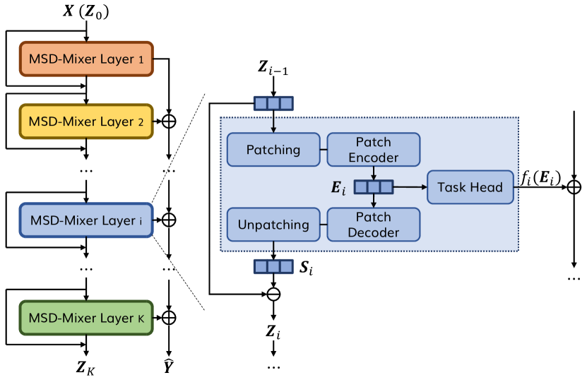
Figure 1: MSD-Mixer overview.

III-C Multi-Scale Temporal Patching

Considering the importance of multi-level sub-series level modeling for time series analysis, we introduce multi-scale temporal patching in MSD-Mixer such that different layers can focus on different sub-series level features. Each layer of MSD-Mixer has a predefined patch size $p_{i}$, which is a hyperparameter to be determined or tuned for specific datasets.

We depict the patching process in Figure 2. To transform an input time series with $C$ channels and $L$ time steps into patches with patch size $p$, we first pad the time series with zeros at the beginning of the time series to ensure the length is divisible by $p$, and then segment the time series along the temporal dimension into non-overlapping patches with stride $p$. We then permute the data to create a new dimension for the patches, resulting in a high dimensional tensor of $C\times L^{\prime}\times p$, where $L^{\prime}=\lceil L/p\rceil$

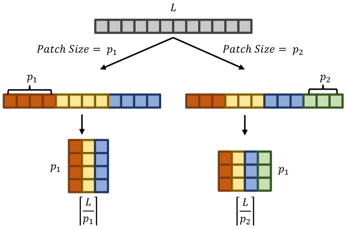
Figure 2: Examples of multi-scale temporal patching. The channel dimension is omitted for simplicity.

III-D Patch Encoder and Decoder

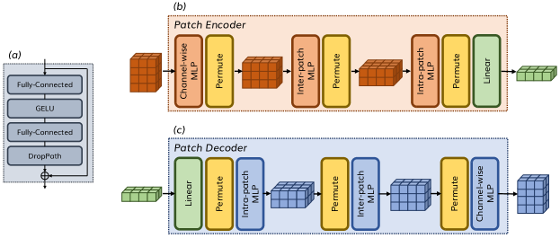
Figure 3: (a) MLP block. (b)Patch Encoder. (c)Patch Decoder.

The Patch Encoder and Decoder modules are based exclusively on MLPs along different dimensions for feature extraction. We show the design of each MLP block in Figure 3(a), which consists of two fully connected layers, a GELU nonlinearity layer, and a DropPath layer [38], together with a residual connection that adds the input to the output. We use the following types of MLP blocks in Patch Encoder and Decoder modules:

• The channel-wise MLP block allows communication between different channels, to capture inter-channel correlations.

• The inter-patch MLP block allows communication between different patches, to capture global contexts.

• The intra-patch MLP block allows communication between different time steps within a patch, to capture sub-series level variations.

As shown in Figure 3(b) the Patch Encoder module consists of a channel-wise MLP block, an inter-patch MLP block, an intra-patch MLP block, and a linear layer in order to produce the component representation $\boldsymbol{E}_{i}$ from the patched $\boldsymbol{Z}_{i-1}$. And the Patch Decoder module (3(c)) consists of the same number and type of blocks as the Patch Encoder module, but in a reversed order to reconstruct $\boldsymbol{S}_{i}$ from $\boldsymbol{E}_{i}$.

III-E Residual Loss

Successful decomposition of a time series usually leaves a white noise as the residual and captures useful information in different components. The most common way to test whether a time series is white noise is to compute its autocorrelation coefficients. The larger the coefficients are, the more information the series still contains. And it is usually expected that the autocorrelation coefficients of a white noise series lie within $\pm 2/\sqrt{L}$ where $L$ is the series length. In this paper, we propose a novel Residual Loss to train MSD-Mixer such that it learns to decompose the input time series completely.

In a MSD-Mixer with $k$ layers, $\boldsymbol{Z}_{k}$ output by the last layer specifies the residual of the decomposition. We first compute the autocorrelation coefficient matrix $\boldsymbol{A}=\{a_{i,j}\}\in\mathbb{R}^{C\times(L-1)}$ of $\boldsymbol{Z}_{k}$ as:

$$a_{i,j}=\frac{\sum_{t=j+1}^{L}(z_{i,t}-\bar{z_{i}})(z_{i,t-j}-\bar{z_{i}})}{\sum_{t=1}^{L}(z_{i,t}-\bar{z_{i}})^{2}},$$ (5)

where $z_{i,j}$ is the $i$-th channel and $j$-th time step of $\boldsymbol{Z}_{k}$. And we then define the Residual Loss by:

$$\mathcal{L}_{r}=\frac{\sum_{i,j}(\mathrm{ReLU}(|a_{i,j}|-\alpha/\sqrt{L}))^{2}}{C\times(L-1)}+\frac{\sum_{i,j}z_{i,j}^{2}}{C\times L}.$$ (6)

The first term of $\mathcal{L}_{r}$ imposes constraint on the autocorrelation coefficients of the residual, where $\alpha$ is a hyperparameter controlling the maximum tolerance of the autocorrelation coefficients. However, it is not enough since it does not minimize the mean of the residual, which carries magnitude information of the input time series. Therefore, in the right term we minimize the mean square of the residual. We finally train MSD-Mixer by simultaneously optimizing the weighted sum of the task-specific loss and the Residual Loss:

$$\mathcal{L}=\mathcal{L}_{t}+\lambda\mathcal{L}_{r}.$$ (7)

III-F Summary

We summarize the overall training process of MSD-Mixer in Algorithm 1. Given a training dataset $\mathcal{D}$ with time series data and corresponding labels as $\mathcal{D}=\{(\boldsymbol{X},\boldsymbol{Y})_{i}\}$, we train MSD-Mixer based on the dataset until the loss converges. During the process, we first sample $(\boldsymbol{X},\boldsymbol{Y})$ from $\mathcal{D}$ (line 3), and then initialize $\boldsymbol{Z}_{0}$ to be $\boldsymbol{X}$ (line 4). After that, for each layer $i\in[1,k]$, we patch $\boldsymbol{Z}_{i-1}$ using the patch size $p_{i}$ (line 6). The patched input is then fed into MLP-Mixer to generate $\boldsymbol{E}_{i}$ (line 7). This learned representation $\boldsymbol{E}_{i}$ is eventually decoded and unpatched to reconstruct the input in each layer (lines 8 – 10). The labels are predicted with loss computed for back propagation (lines 11 – 13). This whole process is repeated until convergence to return the trained MSD-Mixer model (line 14).

Input: Training set $\mathcal{D}=\{(\boldsymbol{X},\boldsymbol{Y})_{i}\}$, number of layers $k$, patch size for each layer $p_{1},\cdots,p_{k}$.

Output: Trained MSD-Mixer.

1 Initialize MSD-Mixer with $k$ layers of patch size $p_{1},\cdots,p_{k}$.

2 repeat

      3 Sample ($\boldsymbol{X}$,$\boldsymbol{Y}$) from $\mathcal{D}$.

      4 $\boldsymbol{Z}_{0}=\boldsymbol{X}$.

      5 for $i=1,2,\ldots,k$ do

            6 Patch $Z_{i-1}$ with $p_{i}$.

            7 Compute $E_{i}=g_{i}(Z_{i-1})$ with $i$-th layer’s Patch Encoder.

            8 Compute $S_{i}=h_{i}(E_{i})$ with $i$-th layer’s Patch Decoder.

            9 Unpatch $S_{i}$ with $p_{i}$.

            10 $\boldsymbol{Z}_{i}=\boldsymbol{Z}_{i-1}-\boldsymbol{S}_{i}$.

       end for

      11Compute $\boldsymbol{\hat{Y}}=\sum_{i=1}^{k}f_{i}(E_{i})$ with Task Head modules.

      12 Computer loss according to Equation 5–7.

      13 Back propagation.

until convergence;

14return Trained MSD-Mixer.

Algorithm 1 Training of MSD-Mixer.

IV Illustrative Experimental Results

In this section, we first overview the experiment setup and key results in Section IV-A. Then, in Section IV-B to IV-E we discuss in detail the experiments and results of different time series analysis tasks, followed by ablation studies on our proposed modules in Section IV-G. Lastly, we empirically analyze the decomposition of MSD-Mixer by example cases in Section IV-H.

IV-A Overview

TABLE I: Summary of Tasks and Benchmarks

Tasks	Datasets [8]	Metrics
Long-Term Forecasting	ETT (4 subsets), Electricity, Weather, Traffic, Exchange	Mean Square Error (MSE), Mean Absolute Error (MAE)
Short-Term Forecasting	M4 (6 subsets)	SMAPE, MASE, OWA [39]
Imputation	ETT (4 subsets), Electricity, Weather	MSE, MAE
Anomaly Detection	SMD, MSL, SMAP, SWaT, PSM	F1-Score
Classification	UEA (10 subsets) [5]	Accuracy

TABLE II: Overall performance comparison in five tasks. Each number of a scheme in the table represents in how many benchmarks the scheme performs best. The best results are in bold and the second bests are underlined.

Task	# of Benchmarks	MSD-Mixer	PatchTST	TimesNet	ETSformer	DLinear	LightTS	NST	FEDformer
		(Ours)	(2023)	(2023)	(2022)	(2023)	(2022)	(2022)	(2022)
Long-Term Forecasting	64	49	7	3	2	3	1	0	3
Short-Term Forecasting	15	15	0	0	0	0	0	0	0
Imputation	48	45	0	9	0	0	0	0	0
Anomaly Detection	5	4	0	1	0	0	0	0	0
Classification	10	5	0	0	0	0	0	0	0
Total	142	118	7	13	2	3	1	0	3

In order to validate the modeling ability of MSD-Mixer, we conduct extensive experiments on a wide range of well-adopted benchmark datasets across five most common time series analysis tasks, including long- and short-term forecasting, imputation, anomaly detection, and classification. The tasks and datasets are of different characteristics and examine different aspects of the model. Table I summarizes the five tasks, datasets, and evaluation metrics we used in the experiments.

We compare our proposed MSD-Mixer with state-of-the-art task-general and task-specific approaches. We select TimesNet [8], PatchTST [9], ETSformer [21], DLinear [11], LightTS [29], Non-stationary Transformer (NST) [40], and FEDformer [16] as task-general baselines for comparison in all the five tasks. Among them, TimesNet is the state-of-the-art task-general approach, and PatchTST is a recent approach that shows impressive performance in time series forecasting and representation learning. The others, although originally proposed for forecasting, have been evaluated by [8] and show good performance on the five tasks. Meanwhile, these approaches have covered mainstream deep learning architectures, including Transformer (PatchTST, ETSformer, NST, FEDformer), CNN (TimesNet), and MLP (DLinear, LightTS), which help to provide a comprehensive view on the time series analysis problem. Furthermore, we include state-of-the-art task-specific approaches into the comparison for the forecasting, anomaly detection, and classification tasks.

We follow well-established experiment setup and implementations of task-general baselines in [8]. All models including MSD-Mixer and baselines are implemented in PyTorch and trained with a single NVIDIA GeForce RTX 3090 GPU with 24GB memory. We search the best number of layers from 4 to 6, and dimensions of the model from 64 to 512 for MSD-Mixer with different datasets. And we set the patch size in MSD-Mixer by considering the series length and sampling interval of the dataset. For instance, in the ETTm1 dataset with input length as 96 and sampling interval as 15 minutes, we use 5 layers with patch sizes as {24, 12, 4, 2, 1}, which correspond to sub-series of 6 hours, 3 hours, 1 hour, 30 minutes, and 15 minutes. We arrange the layers in MSD-Mixer with their patch sizes in descending order.

Table II summarizes the overall performance of task-general schemes. As shown in the table, our proposed MSD-Mixer outperforms other state-of-the-art algorithms significantly in all the benchmarks across the five tasks. We can see that MSD-Mixer is far ahead of the others by a large margin, which demonstrates the great and comprehensive ability of MSD-Mixer for time series analysis.

IV-B Long-Term Forecasting

TABLE III: Statistics of datasets for long-term forecasting.

Dataset	Dim	Total Timesteps	Frequency
ETTm1, ETTm2	7	69680	15 mins
ETTh1, ETTh2	7	17420	1 hour
ECL	321	26304	10 mins
Traffic	862	17544	1 hour
Weather	21	52696	10 mins
Exchange	8	7588	1 day

Time series forecasting has always been the primary goal of time series analysis, while the long-term forecasting problem is characterized by the extraordinary long forecasting horizon as output, which puts emphasis on the ability of long-range modeling. In this task, we evaluate the approaches on eight popular real-world datasets across energy, transportation, weather, and finance domains. Information of the datasets is summarized in Table III. For each dataset, we set the length of look-back window as 96, and train each approach with four forecasting horizons of 96, 192, 336, and 720, respectively, to evaluate the performance under different forecasting horizons. Since each dataset only contains one long multivariate time series, we obtain input and output sample pairs by sliding window. Furthermore, we include Scaleformer [37] as a task-specific approach in the long-term forecasting experiments. Scaleformer is a recent Transformer-based approach with good performance in long-term forecasting which is featured by iteratively refining the forecasting result at multiple scales. We use the mean squared error (MSE) and mean absolute error (MAE) to evaluate the performance of multivariate forecasting.

As shown in Table IV, MSD-Mixer achieves the best performance on most datasets, including different forecasting horizon settings, with the 49 first and 7 second places out of 64 benchmarks in total. Furthermore, on most leading metrics, MSD-Mixer outperforms the second place by a significant margin. From the results, we can see that although ETSformer adopts the decomposition design, it still bases on point-wise self-attention for temporal feature extraction, which has been shown to be ineffective for sub-series modeling, therefore it struggles to outperform even the DLinear baseline which is just a simple linear projection. FEDformer, TimesNet, and PatchTST all considers simple series-trend decomposition on the model input, which brings about some advantage to them. TimesNet and PatchTST further consider sub-series modeling in their design, therefore these two schemes are shown to be the strongest baselines. Compared with them, MSD-Mixer combines decomposition with multi-scale sub-series modeling. We believe the great performance of MSD-Mixer fully demonstrates the efficacy of our multi-scale decomposition in time series modeling.

TABLE IV: Long-term forecasting results. The best results are in bold and the second bests are underlined.

Models		MSD-Mixer		PatchTST		Scaleformer		TimesNet		ETSformer		DLinear		LightTS		NST		FEDformer
		(Ours)		(2023)		(2023)		(2023)		(2022)		(2023)		(2022)		(2022)		(2022)
Metric		MSE	MAE	MSE	MAE	MSE	MAE	MSE	MAE	MSE	MAE	MSE	MAE	MSE	MAE	MSE	MAE	MSE	MAE
ETTm1	96	0.304	0.351	0.334	0.372	0.392	0.415	0.338	0.375	0.375	0.398	0.345	0.372	0.374	0.400	0.386	0.398	0.379	0.419
	192	0.344	0.375	0.378	0.394	0.437	0.451	0.374	0.387	0.408	0.410	0.380	0.389	0.400	0.407	0.459	0.444	0.426	0.441
	336	0.370	0.395	0.406	0.414	0.499	0.478	0.410	0.411	0.435	0.428	0.413	0.413	0.438	0.438	0.495	0.464	0.445	0.459
	720	0.427	0.428	0.462	0.445	0.584	0.536	0.478	0.450	0.499	0.462	0.474	0.453	0.527	0.502	0.585	0.516	0.543	0.490
ETTm2	96	0.169	0.259	0.175	0.259	0.182	0.276	0.187	0.267	0.189	0.280	0.193	0.292	0.209	0.308	0.192	0.274	0.203	0.287
	192	0.232	0.300	0.240	0.302	0.252	0.319	0.249	0.309	0.253	0.319	0.284	0.362	0.311	0.382	0.280	0.339	0.269	0.328
	336	0.292	0.337	0.302	0.342	0.335	0.372	0.321	0.351	0.314	0.357	0.369	0.427	0.442	0.466	0.334	0.361	0.325	0.366
	720	0.392	0.398	0.399	0.397	0.460	0.446	0.408	0.403	0.414	0.413	0.554	0.522	0.675	0.587	0.417	0.413	0.421	0.415
ETTh1	96	0.377	0.391	0.444	0.438	0.404	0.441	0.384	0.402	0.494	0.479	0.386	0.400	0.424	0.432	0.513	0.491	0.376	0.419
	192	0.427	0.422	0.488	0.463	0.438	0.461	0.436	0.429	0.538	0.504	0.437	0.432	0.475	0.462	0.534	0.504	0.420	0.448
	336	0.469	0.443	0.525	0.484	0.464	0.477	0.491	0.469	0.574	0.521	0.481	0.459	0.518	0.488	0.588	0.535	0.459	0.465
	720	0.485	0.475	0.532	0.510	0.507	0.516	0.521	0.500	0.562	0.535	0.519	0.516	0.547	0.533	0.643	0.616	0.506	0.507
ETTh2	96	0.284	0.345	0.312	0.358	0.335	0.385	0.340	0.374	0.340	0.391	0.333	0.387	0.397	0.437	0.476	0.458	0.358	0.397
	192	0.362	0.392	0.401	0.410	0.455	0.451	0.402	0.414	0.430	0.439	0.477	0.476	0.520	0.504	0.512	0.493	0.429	0.439
	336	0.399	0.428	0.437	0.442	0.477	0.479	0.452	0.452	0.485	0.479	0.594	0.541	0.626	0.559	0.552	0.551	0.496	0.487
	720	0.426	0.457	0.442	0.454	0.467	0.490	0.462	0.468	0.500	0.497	0.831	0.657	0.863	0.672	0.562	0.560	0.463	0.474
Electricity	96	0.152	0.254	0.211	0.312	0.182	0.297	0.168	0.272	0.187	0.304	0.197	0.282	0.207	0.307	0.169	0.273	0.193	0.308
	192	0.165	0.263	0.214	0.313	0.188	0.300	0.184	0.289	0.199	0.315	0.196	0.285	0.213	0.316	0.182	0.286	0.201	0.315
	336	0.173	0.273	0.230	0.328	0.210	0.324	0.198	0.300	0.212	0.329	0.209	0.301	0.230	0.333	0.200	0.304	0.214	0.329
	720	0.201	0.299	0.272	0.359	0.232	0.339	0.220	0.320	0.233	0.345	0.245	0.333	0.265	0.360	0.222	0.321	0.246	0.355
Traffic	96	0.500	0.324	0.579	0.388	0.564	0.351	0.593	0.321	0.607	0.392	0.650	0.396	0.615	0.391	0.612	0.338	0.587	0.366
	192	0.506	0.324	0.571	0.382	0.570	0.349	0.617	0.336	0.621	0.399	0.598	0.370	0.601	0.382	0.613	0.340	0.604	0.373
	336	0.528	0.341	0.582	0.385	0.576	0.349	0.629	0.336	0.622	0.396	0.605	0.373	0.613	0.386	0.618	0.328	0.621	0.383
	720	0.561	0.369	0.596	0.389	0.602	0.360	0.640	0.350	0.632	0.396	0.645	0.394	0.658	0.407	0.653	0.355	0.626	0.382
Weather	96	0.148	0.212	0.180	0.222	0.220	0.289	0.172	0.220	0.197	0.281	0.196	0.255	0.182	0.242	0.173	0.223	0.217	0.296
	192	0.200	0.262	0.229	0.261	0.341	0.385	0.219	0.261	0.237	0.312	0.237	0.296	0.227	0.287	0.245	0.285	0.276	0.336
	336	0.256	0.310	0.281	0.298	0.463	0.455	0.280	0.306	0.298	0.353	0.283	0.335	0.282	0.334	0.321	0.338	0.339	0.380
	720	0.327	0.362	0.358	0.349	0.682	0.565	0.365	0.359	0.352	0.288	0.345	0.381	0.352	0.386	0.414	0.410	0.403	0.428
Exchange	96	0.085	0.203	0.085	0.202	0.109	0.240	0.107	0.234	0.085	0.204	0.088	0.218	0.116	0.262	0.111	0.237	0.148	0.278
	192	0.176	0.297	0.180	0.301	0.241	0.353	0.226	0.344	0.182	0.303	0.176	0.315	0.215	0.359	0.219	0.335	0.271	0.380
	336	0.336	0.418	0.336	0.420	0.471	0.508	0.367	0.448	0.348	0.428	0.313	0.427	0.377	0.466	0.421	0.476	0.460	0.500
	720	0.953	0.738	0.881	0.710	1.259	0.865	0.964	0.746	1.025	0.774	0.839	0.695	0.831	0.699	1.092	0.769	1.195	0.841
1st Count		49		7		0		3		2		3		1		0		3

IV-C Short-Term Forecasting

TABLE V: Statistics of datasets for short-term forecasting.

Dataset	Dim	Series Length	Training Set Size	Test Set Size
Yearly	1	6	23000	23000
Quarterly	1	8	24000	24000
Monthly	1	18	48000	48000
Weekly	1	13	359	359
Daily	1	14	4227	4227
Hourly	1	48	414	414

TABLE VI: Short-term forecasting results. The best results are in bold and the second bests are underlined.

Models		MSD-Mixer	N-HiTS	N-BEATS	PatchTST	TimesNet	ETSformer	DLinear	LightTS	NST	FEDformer
		(Ours)	(2023)	(2020)	(2023)	(2023)	(2022)	(2023)	(2022)	(2022)	(2022)
Yearly	SMAPE	13.191	13.418	13.436	13.777	13.387	18.009	16.965	14.247	13.717	13.728
	MASE	2.967	3.045	3.043	3.056	2.996	4.487	4.283	3.109	3.078	3.048
	OWA	0.777	0.793	0.794	0.806	0.786	1.115	1.058	0.827	0.807	0.803
Quarterly	SMAPE	9.971	10.202	10.124	11.058	10.100	13.376	12.145	11.364	10.958	10.792
	MASE	1.151	1.194	1.169	1.321	1.182	1.906	1.520	1.328	1.325	1.283
	OWA	0.872	0.899	0.886	0.984	0.890	1.302	1.106	1.000	0.981	0.958
Monthly	SMAPE	12.588	12.791	12.677	14.433	12.670	14.588	13.514	14.014	13.917	14.260
	MASE	0.921	0.969	0.937	1.154	0.933	1.368	1.037	1.053	1.097	1.102
	OWA	0.869	0.899	0.880	1.043	0.878	1.149	0.956	0.981	0.998	1.012
Others	SMAPE	4.615	5.061	4.925	5.216	4.891	7.267	6.709	15.880	6.302	4.954
	MASE	3.124	3.216	3.391	3.688	3.302	5.240	4.953	11.434	4.064	3.264
	OWA	0.978	1.040	1.053	1.130	1.035	1.591	1.487	3.474	1.304	1.036
W. Avg.	SMAPE	11.700	11.927	11.851	13.011	11.829	14.718	13.639	13.525	12.780	12.840
	MASE	1.557	1.613	1.599	1.758	1.585	2.408	2.095	2.111	1.756	1.701
	OWA	0.838	0.861	0.855	0.939	0.851	1.172	1.051	1.051	0.930	0.918

In the short-term forecasting task, we adopt the dataset and performance measures of the well-known M4 Competition [39], which focus on the short-term forecasting of univariate time series in contrast to the long-term forecasting task. The dataset contains 100000 time series data in total, which are further divided into 6 subsets by sampling intervals including yearly, quarterly monthly, weekly, daily, and hourly. More information of the dataset is given in Table V. Each subset contains real-life time series data from economics, finance, industry, demographic, and other domains, which requires the forecasting models to learn general temporal patterns from samples across diverse domains. In this task, we include N-BEATS [19] and N-HiTS [20] as task-specific methods. The forecasting results are evaluated by the symmetric mean absolute percentage error (SMAPE), mean absolute scaled error (MASE), which can be calculated as:

$$\mathrm{SMAPE}= \frac{200}{H}\sum_{i=1}^{H}\frac{|y_{i}-\hat{y_{i}}|}{|y_{i}|+|\hat{y_{i}}|},$$ (8)

$$\mathrm{MASE}= \frac{1}{H}\sum_{i=1}^{H}\frac{|y_{i}-\hat{y_{i}}|}{\frac{1}{H-m}\sum_{j=m+1}^{H}|y_{j}-y_{h-m}|},$$

$$\mathrm{OWA}= \frac{1}{2}\left[\frac{\mathrm{SMAPE}}{\mathrm{SMAPE}_{Naive2}}+\frac{\mathrm{MASE}}{\mathrm{MASE}_{Naive2}}\right],$$

where $y_{i}$ and $\hat{y_{i}}$ are the ground truth and forecasting of the $i$-th time step in $H$ total future time steps, $m$ is the periodicity of the data. $\mathrm{SMAPE}_{Naive2}$ and $\mathrm{MASE}_{Naive2}$ are SMAPE and MASE of a baseline method provided in the competition. And we follow the official settings of the competition to compute the weighted average over different subsets for overall evaluation in this task.

As shown in Table VI, MSD-Mixer again leads the board with top-1 performance in every benchmark, which demonstrates the excellent capability of MSD-Mixer on modeling short and univariate time series. Each time point in a univariate time series is a single scalar, which makes it even harder for Transformer based model to attain meaningful attention score. Therefore, Transformer based approaches have inferior performance in this task, especially ETSformer which is without sub-series level modeling. Among the baselines, N-HiTS and N-BEATS are based on explicit decomposition, and they show satisfactory performance in this task, which validates the effectiveness of decomposition for time series modeling. MSD-Mixer further advances N-BEATS and N-HiTS with multi-scale temporal patching and mixing, as well as the Residual Loss for better extraction of temporal patterns, which facilitates MSD-Mixer with stronger modeling ability than them, and helps MSD-Mixer achieve the best performance.

IV-D Imputation

TABLE VII: Imputation results. The best results are in bold and the second bests are underlined.

Models		MSD-Mixer		PatchTST		TimesNet		ETSformer		DLinear		LightTS		NST		FEDformer
		(Ours)		(2023)		(2023)		(2022)		(2023)		(2022)		(2022)		(2022)
Metric		MSE	MAE	MSE	MAE	MSE	MAE	MSE	MAE	MSE	MAE	MSE	MAE	MSE	MAE	MSE	MAE
ETTm1	12.5%	0.019	0.096	0.047	0.138	0.019	0.092	0.067	0.188	0.058	0.162	0.075	0.180	0.026	0.107	0.035	0.135
	25%	0.019	0.092	0.040	0.127	0.023	0.101	0.096	0.229	0.080	0.193	0.093	0.206	0.032	0.119	0.052	0.166
	37.5%	0.024	0.103	0.043	0.132	0.029	0.111	0.133	0.271	0.103	0.219	0.113	0.231	0.039	0.131	0.069	0.191
	50%	0.027	0.103	0.048	0.139	0.036	0.124	0.186	0.323	0.132	0.248	0.134	0.255	0.047	0.145	0.089	0.218
ETTm2	12.5%	0.018	0.079	0.026	0.093	0.018	0.080	0.108	0.239	0.062	0.166	0.034	0.127	0.021	0.088	0.056	0.159
	25%	0.020	0.084	0.026	0.094	0.020	0.085	0.164	0.294	0.085	0.196	0.042	0.143	0.024	0.096	0.080	0.195
	37.5%	0.022	0.091	0.033	0.110	0.023	0.091	0.237	0.356	0.106	0.222	0.051	0.159	0.027	0.103	0.110	0.231
	50%	0.026	0.100	0.033	0.106	0.026	0.098	0.323	0.421	0.131	0.247	0.059	0.174	0.030	0.108	0.156	0.276
ETTh1	12.5%	0.031	0.116	0.081	0.189	0.057	0.159	0.126	0.263	0.151	0.267	0.240	0.345	0.060	0.165	0.070	0.190
	25%	0.041	0.135	0.093	0.202	0.069	0.178	0.169	0.304	0.180	0.292	0.265	0.364	0.080	0.189	0.106	0.236
	37.5%	0.056	0.157	0.104	0.214	0.084	0.196	0.220	0.347	0.215	0.318	0.296	0.382	0.102	0.212	0.124	0.258
	50%	0.071	0.179	0.124	0.232	0.102	0.215	0.293	0.402	0.257	0.347	0.334	0.404	0.133	0.240	0.165	0.299
ETTh2	12.5%	0.037	0.125	0.059	0.152	0.040	0.130	0.187	0.319	0.100	0.216	0.101	0.231	0.042	0.133	0.095	0.212
	25%	0.040	0.131	0.059	0.154	0.046	0.141	0.279	0.390	0.127	0.247	0.115	0.246	0.049	0.147	0.137	0.258
	37.5%	0.048	0.145	0.064	0.161	0.052	0.151	0.400	0.465	0.158	0.276	0.126	0.257	0.056	0.158	0.187	0.304
	50%	0.058	0.163	0.070	0.170	0.060	0.162	0.602	0.572	0.183	0.299	0.136	0.268	0.065	0.170	0.232	0.341
Electricity	12.5%	0.048	0.150	0.103	0.215	0.085	0.202	0.196	0.321	0.092	0.214	0.102	0.229	0.093	0.210	0.107	0.237
	25%	0.059	0.170	0.105	0.219	0.089	0.206	0.207	0.332	0.118	0.247	0.121	0.252	0.097	0.214	0.120	0.251
	37.5%	0.070	0.184	0.109	0.225	0.094	0.213	0.219	0.344	0.144	0.276	0.141	0.273	0.102	0.220	0.136	0.266
	50%	0.080	0.197	0.113	0.231	0.100	0.221	0.235	0.357	0.175	0.305	0.160	0.293	0.108	0.228	0.158	0.284
Weather	12.5%	0.025	0.043	0.043	0.069	0.025	0.045	0.057	0.141	0.039	0.084	0.047	0.101	0.027	0.051	0.041	0.107
	25%	0.028	0.050	0.041	0.065	0.029	0.052	0.065	0.155	0.048	0.103	0.052	0.111	0.029	0.056	0.064	0.163
	37.5%	0.030	0.049	0.043	0.069	0.031	0.057	0.081	0.180	0.057	0.117	0.058	0.121	0.033	0.062	0.107	0.229
	50%	0.033	0.056	0.045	0.070	0.034	0.062	0.102	0.207	0.066	0.134	0.065	0.133	0.037	0.068	0.183	0.312
1st Count		45		0		9		0		0		0		0		0

Missing values are common in real-world continuous data systems that collect time series data from various sources. A single missing data in a time series can invalid the whole downstream application since most analysis methods assume complete data, which makes missing data imputation critical for time series analysis. In this task, we experiment on the ETT, Electricity, and Weather datasets which we have used in long-term forecasting (Table III). In each experiment, we generate the training data by random mask with zeros as input, and use the unmasked data as label for training and testing. To evaluate the performance under different ratios of missing data, for each dataset we train and evaluate each method with four missing data ratios of 12.5%, 25%, 37.5%, and 50%, respectively. We calculate the MSE and MAE of the imputed missing values and the corresponding ground truth as metrics. Due to missing data in the input, it is not feasible to compute the autocorrelation of the residual. Therefore, we only compute the mean square error of the residual in the Residual Loss.

Results in Table VII show that MSD-Mixer also achieves the best performance on most datasets, as well as on different missing data ratios, with the 45 first place out of 48 benchmarks in total. This task requires the model to learn correct temporal patterns from the data with missing values masked as zeros, which is challenging for most models. We observe that MSD-Mixer and TimesNet, which shows good performance in this task, have both considered sub-series modeling in multiple timescales. From this, we think sub-series modeling may help provide local context information for the estimation of missing values. Meanwhile, MSD-Mixer performs much better than TimesNet. This is because MSD-Mixer also considers multi-scale decomposition of the time series. It disentangles the temporal patterns within the data, such that they can be better modeled for the estimation of the missing value. Furthermore, the performance of other baseline methods drops quickly as the missing ratio increases, whereas the performance of our MSD-Mixer remains more stable, and consistently better than others. This also highlights the excellent capability of MSD-Mixer to model temporal patterns in complex time series data.

IV-E Anomaly Detection

TABLE VIII: Statistics of datasets for anomaly detection.

Dataset	Dim	Series Length	Training Set Size	Test Set Size
SMD	38	100	708405	708420
MSL	55	100	58317	73729
SMAP	25	100	135183	427617
SWaT	51	100	495000	449919
PSM	25	100	132481	87841

TABLE IX: Anomaly detection results. The best results are in bold and the second bests are underlined.

Models		MSD-Mixer	Anomaly	PatchTST	TimesNet	ETSformer	DLinear	LightTS	NST	FEDformer
		(Ours)	(2021)	(2023)	(2023)	(2022)	(2023)	(2022)	(2022)	(2022)
SMD	Precision	88.7	88.9	87.5	88.7	87.4	83.6	87.1	88.3	88.0
	Recall	86.1	82.2	82.2	83.1	79.2	71.5	78.4	81.2	82.4
	F1-score	87.4	85.5	84.7	85.8	83.1	77.1	82.5	84.6	85.1
MSL	Precision	91.3	79.6	87.4	83.9	85.1	84.3	82.4	68.6	77.1
	Recall	88.4	87.4	69.5	86.4	84.9	85.4	75.8	89.1	80.1
	F1-score	89.8	83.3	77.4	85.2	85.0	84.9	79.0	77.5	78.6
SMAP	Precision	93.4	91.9	90.5	92.5	92.3	92.3	92.6	89.4	90.5
	Recall	96.9	58.1	56.4	58.3	55.8	55.4	55.3	59.0	58.1
	F1-score	95.2	71.2	69.5	71.5	69.5	69.3	69.2	71.1	70.8
SwaT	Precision	93.1	72.5	91.3	86.8	90.0	80.9	92.0	68.0	90.2
	Recall	98.3	97.3	83.2	97.3	80.4	95.3	94.7	96.8	96.4
	F1-score	95.7	83.1	87.1	91.7	84.9	87.5	93.3	79.9	93.2
PSM	Precision	97.4	68.4	98.9	98.2	99.3	98.3	98.4	97.8	97.3
	Recall	96.7	94.7	92.4	96.8	85.3	89.3	96.0	96.8	97.2
	F1-score	97.0	79.4	95.6	97.5	91.8	93.6	97.2	97.3	97.2
Average F1-score		93.0	80.0	82.8	86.3	86.2	83.8	84.2	83.2	85.0

Anomaly detection of time series data is of immense value in many real-time monitoring applications. It is also challenging due to the lack of labeled data. In this task, we consider the reconstruction-based unsupervised anomaly detection which are widely applied for time series. On this premise, the models learn to represent and reconstruct the normal data, thus abnormal time points can be detected with large reconstruction error [4]. Therefore, this task is quite challenging about the quality of the representation learned by the model. In this task, we experiment on five widely-adopted time series anomaly detection datasets. Information of the datasets is summarized in Table VIII. We include [4] as a task-specific baseline method following [8] for comprehensive and fair comparison. We calculate and report the point-wise precision, recall, and F1-score of the detection result, and use F1-score to compare the performance of different methods.

As shown in Table IX, MSD-Mixer achieves the best F1-score in 4 out of the 5 datasets. It also has the best averaged F1-score over all datasets. Compared with the baselines that simply learns to represent and reconstruct the time series, MSD-Mixer further learns to explicitly decompose the time series into components and represent each component for the reconstruction. Thus MSD-Mixer has stronger representation learning ability to precisely capture the normal temporal pattern, and identify the abnormal data.

IV-F Classification

TABLE X: Statistics of datasets for classification.

Dataset	Dim	Series Length	Classes	Training Set Size	Test Set Size
AWR	9	144	25	275	300
AF	2	640	3	15	15
CT	3	182	20	1,422	1,436
CR	6	1,197	12	108	72
FD	144	62	2	5,890	3,524
FM	28	50	2	316	100
MI	64	3,000	2	278	100
SCP1	6	896	2	268	293
SCP2	7	1,152	2	200	180
UWGL	3	315	8	120	320

TABLE XI: Classification results. The best results are in bold and the second bests are underlined.

Models	MSD-Mixer	TARNet	DTWD	TapNet	MiniRocket	TST	FormerTime	PatchTST	TimesNet	DLinear	ETSformer	LightTS	NST	FEDformer
	(Ours)	(2022)	(2015)	(2020)	(2021)	(2021)	(2023)	(2023)	(2023)	(2023)	(2022)	(2022)	(2022)	(2022)
AWR	0.983	0.977	0.987	0.987	0.993	0.947	0.985	0.040	0.977	0.963	0.973	0.970	0.497	0.587
AF	0.600	1.000	0.220	0.333	0.133	0.533	0.600	0.467	0.333	0.200	0.400	0.333	0.467	0.400
CT	0.987	0.994	0.989	0.997	0.990	0.971	0.991	0.877	0.974	0.973	0.978	0.977	0.804	0.960
CR	1.000	1.000	1.000	0.958	0.986	0.847	0.981	0.083	0.847	0.861	0.861	0.847	0.736	0.472
FD	0.698	0.641	0.529	0.556	0.612	0.625	0.687	0.500	0.686	0.672	0.673	0.658	0.500	0.684
FM	0.660	0.620	0.530	0.530	0.550	0.590	0.618	0.510	0.590	0.570	0.590	0.540	0.510	0.540
MI	0.670	0.630	0.500	0.590	0.610	0.610	0.632	0.570	0.570	0.620	0.590	0.590	0.640	0.580
SCP1	0.949	0.816	0.775	0.652	0.915	0.961	0.887	0.741	0.918	0.880	0.860	0.918	0.898	0.594
SCP2	0.639	0.622	0.539	0.550	0.506	0.604	0.592	0.500	0.572	0.527	0.561	0.522	0.500	0.511
UWGL	0.884	0.878	0.903	0.894	0.785	0.913	0.888	0.213	0.853	0.812	0.825	0.831	0.703	0.453
Avg. Acc.	0.807	0.818	0.697	0.705	0.708	0.760	0.786	0.450	0.732	0.708	0.731	0.719	0.625	0.578
1st Count	5	3	1	1	1	2	0	0	0	0	0	0	0	0
Mean Rank	2.8	4.4	8	7.5	7.6	6.3	3.7	12.8	7.1	8.6	7.2	8.1	10.3	10.6

The time series classification problem arises in various real-life applications such as the human activity recognition and medical time series based diagnosis. In this task we consider the series-level classification problem, which involves building predictive models that predict one categorical label from each time series, which emphasize more on discriminative modeling ability of the model in comparison with other time series analysis tasks. We experiment on ten datasets from the well-known UEA time series classification archive [41] which is the most widely used multivariate time series classification benchmark. The ten datasets have diverse characteristics in terms of domain, series length, number of samples, and the number of classes, which helps to comprehensively examine the capabilities of different methods. And the datasets have been well processed and split into train and test sets. Information of the datasets is summarized in Table X. Furthermore, we select another six competitive classification-specific methods reported in recent works [5, 42] as task-specific baselines for comparison in this task. These methods cover both statistical (DTWD [43], MiniRocket [44]) and deep learning (TARNet [42], FormerTime [5], TST [45], TapNet [46]) methods. We use the classification accuracy as our performance metric. Meanwhile, the inclusion of so many baselines makes it even harder for one single model to outperform all other methods on every dataset. Therefore, we also present the Mean Rank which is the average rank of a model across all datasets for comparison.

Table XI shows the result of our classification tests. MSD-Mixer performs the best on 5 first and 2 second place out of 10 benchmarks, which demonstrates good discriminative modeling ability of MSD-Mixer. On the other hand, the diversity of datasets in terms of size, dimension, length, and number of classes also reflects adaptability of MSD-Mixer. Different from other tasks discussed above, the task-general baselines generally perform inferior to task-specific ones in classification. The two strongest baselines are TARNet and TST, which are two Transformer-based deep learning approaches. We also note that two statistical baselines DTWD and MiniRocket also perform well in some datasets. These results indicate that it is challenging to design a task-general backbone for classification tasks. We think fully considering the special composition and multi-scale nature of time series are the reasons why MSD-Mixer can consistently have better performance in classification.

IV-G Ablation Study

TABLE XII: Average results of MSD-Mixer variants on five tasks.

Model		MSD-Mixer	MSD-Mixer-I	MSD-Mixer-N	MSD-Mixer-U	MSD-Mixer-L
Long-Term Forecasting	MSE	0.345	0.345	0.358	0.422	0.348
	MAE	0.358	0.357	0.371	0.470	0.360
Short-Term Forecasting	SMAPE	11.700	11.699	11.814	11.869	11.780
	MASE	1.557	1.557	1.598	1.587	1.567
	OWA	0.838	0.837	0.853	0.853	0.844
Imputation	MSE	0.038	0.039	0.041	0.058	0.040
	MAE	0.117	0.130	0.122	0.149	0.119
Anomaly Detection	F1	0.930	0.925	0.918	0.847	0.897
Classification	ACC	0.807	0.803	0.732	0.729	0.768

We strongly believe that the advantages of MSD-Mixer are rooted in our proposed multi-scale temporal patching and Residual Loss. To validate the efficacy of the proposed components, we implement the following variants of MSD-Mixer:

• MSD-Mixer-I: the inverted MSD-Mixer. We arrange the layers with their patch sizes in ascending order instead of descending.

• MSD-Mixer-N the MSD-Mixer without patching. We substitute the patching modules in with max pooling and linear interpolation layers as specified in [20], respectively.

• MSD-Mixer-U: the MSD-Mixer without multi-scale patching. We set the patch size as the square root of the input length and use this same patch size for all layers.

• MSD-Mixer-L: the MSD-Mixer trained without the Residual Loss.

We carry out experiments for the four MSD-Mixer variants on all benchmarks in the five tasks, and report their average performance over the benchmarks in each task as shown in Table XII. MSD-Mixer-I has very similar performance to the original MSD-Mixer in all five tasks. This result indicates that the arrangement of layers with different patch sizes does not affect the performance of MSD-Mixer. We think the reason behind is that the multi-scale temporal patching makes the layer to focus on the modeling of specific timescale, such that their order has a relatively small impact on the performance. Without the patching modules, MSD-Mixer-N cannot capture the sub-series features, thus we can observe a performance drop compared with MSD-Mixer, especially in classification accuracy. Likewise, by using the same patch size in all layers, MSD-Mixer-U does not model the multi-scale patterns as inductive bias in different layers, which affects the performance considerably in all tasks. Lastly, by comparing MSD-Mixer-L with MSD-Mixer we find that the Residual Loss do contributes to the learning of the model in all tasks, by enhancing the completeness of the decomposition.

IV-H Case Study

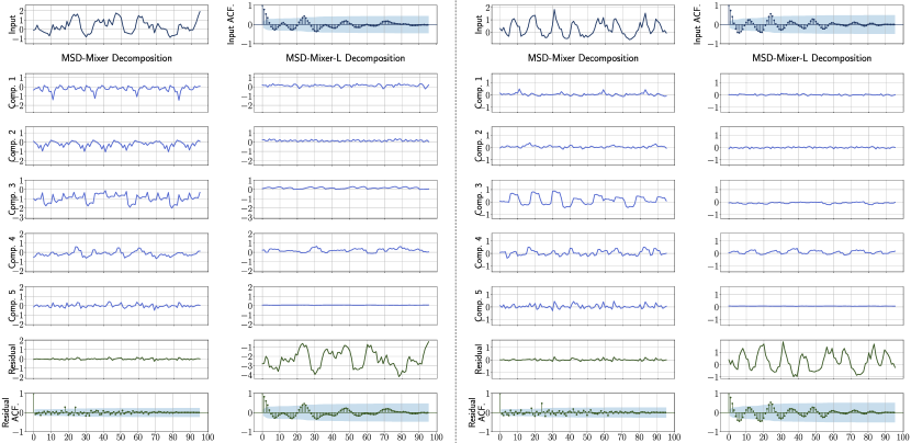
Figure 4: Examples of decomposition.

To further validate the effectiveness of our carefully designed Residual Loss in MSD-Mixer, in Figure 4 we show two examples of how the input time series is decomposed by MSD-Mixer trained with (MSD-Mixer) and without (MSD-Mixer-L) our proposed Residual Loss. The examples are from the long-term forecasting task with the ETTh1 dataset, which is well acknowledged as a challenging dataset with complex characteristics including but not limited to multiple periodic variations and channel-wise heterogeneity. The sampling rate of the data is 1 hour, and input length is set to 96. We train the MSD-Mixer which has 5 layers with patch sizes as {24, 12, 6, 2, 1}, corresponding to sub-sereis of 1 day, half day, 6 hours, 2 hours, and 1 hour.

First, from both input plots we observe multiple irregular temporal patterns, which cannot be simply explained by seasonal or trend-cyclic patterns as discussed in previous works [15]. Their corresponding autocorrelation function (ACF) plots also indicate high correlations in multiple temporal lags in the input data. Therefore, simply considering seasonal-trend decomposition is not enough to account for intricate temporal patterns in real-life time series data. Then, we note that the components output by MSD-Mixer are obviously different, especially in terms of their timescale, which indicates that they contain different temporal patterns in the input data. We attribute it to the effectiveness of our proposed multi-scale temporal patching. Furthermore, it is obvious from both examples that without our proposed Residual Loss, MSD-Mixer-L leaves most of the information from the input in the decomposition residual, while the other components contain little information. In comparison, the magnitudes of residuals from MSD-Mixer are much smaller, and the residual ACF plots also indicates less periodic patterns. The result clearly demonstrates the effectiveness of our proposed Residual Loss is constraining the decomposition residual. The multi-scale components also show the potential to provide interpretability on the composition of the input data and how the output are produced by MSD-Mixer.

V Conclusion

In this work, we seek to solve the time series analysis problem by considering its unique composition and complex multi-scale temporal variations, and propose MSD-Mixer, a Multi-Scale Decomposition MLP-Mixer which learns to explicitly decompose the input time series into different components, and represents the components in different layers. We propose a novel multi-scale temporal patching approach in MSD-Mixer to model the time series as multi-scale sub-series level patches, and employ MLPs along different dimensions to mix intra- and inter-patch variations and channel-wise correlations. In addition, we propose a Residual Loss to constrain both the magnitude and autocorrelation of the decomposition residual for decomposition completeness. Through extensive experiments on 26 real-world datasets, we demonstrate that MSD-Mixer consistently outperforms the state-of-the-art task-general and task-specific approaches by a wide margin on five common tasks, namely long-term forecasting (up to 9.8% in MSE), short-term forecasting (up to 5.6% in OWA), imputation (up to 46.1% in MSE), anomaly detection (up to 33.1% in F1-score) and classification (up to 6.5% in accuracy).

References

- [1] G. Li, S. Zhong, X. Deng, L. Xiang, S.-H. G. Chan, R. Li, Y. Liu, M. Zhang, C.-C. Hung, and W.-C. Peng, “A lightweight and accurate spatial-temporal transformer for traffic forecasting,” IEEE Transactions on Knowledge and Data Engineering, 2022.
- [2] X. Miao, Y. Wu, J. Wang, Y. Gao, X. Mao, and J. Yin, “Generative semi-supervised learning for multivariate time series imputation,” in Proceedings of the AAAI conference on artificial intelligence, vol. 35, no. 10, 2021, pp. 8983–8991.
- [3] H. Ren, B. Xu, Y. Wang, C. Yi, C. Huang, X. Kou, T. Xing, M. Yang, J. Tong, and Q. Zhang, “Time-series anomaly detection service at microsoft,” in Proceedings of the 25th ACM SIGKDD international conference on knowledge discovery & data mining, 2019, pp. 3009–3017.
- [4] J. Xu, H. Wu, J. Wang, and M. Long, “Anomaly transformer: Time series anomaly detection with association discrepancy,” in International Conference on Learning Representations, 2021.
- [5] M. Cheng, Q. Liu, Z. Liu, Z. Li, Y. Luo, and E. Chen, “Formertime: Hierarchical multi-scale representations for multivariate time series classification,” in Proceedings of the ACM Web Conference 2023, 2023, pp. 1437–1445.
- [6] M. West, “Time series decomposition,” Biometrika, vol. 84, no. 2, pp. 489–494, 1997.
- [7] R. J. Hyndman and G. Athanasopoulos, Forecasting: principles and practice. OTexts, 2018.
- [8] H. Wu, T. Hu, Y. Liu, H. Zhou, J. Wang, and M. Long, “Timesnet: Temporal 2d-variation modeling for general time series analysis,” in The Eleventh International Conference on Learning Representations, 2023.
- [9] Y. Nie, N. H. Nguyen, P. Sinthong, and J. Kalagnanam, “A time series is worth 64 words: Long-term forecasting with transformers,” arXiv preprint arXiv:2211.14730, 2023.
- [10] H. Wang, J. Peng, F. Huang, J. Wang, J. Chen, and Y. Xiao, “Micn: Multi-scale local and global context modeling for long-term series forecasting,” in The Eleventh International Conference on Learning Representations, 2023.
- [11] A. Zeng, M. Chen, L. Zhang, and Q. Xu, “Are transformers effective for time series forecasting?” in Proceedings of the AAAI conference on artificial intelligence, vol. 37, no. 9, 2023, pp. 11 121–11 128.
- [12] Y. Zhang and J. Yan, “Crossformer: Transformer utilizing cross-dimension dependency for multivariate time series forecasting,” in The Eleventh International Conference on Learning Representations, 2023.
- [13] L. Han, H.-J. Ye, and D.-C. Zhan, “The capacity and robustness trade-off: Revisiting the channel independent strategy for multivariate time series forecasting,” 2023.
- [14] A. Vaswani, N. Shazeer, N. Parmar, J. Uszkoreit, L. Jones, A. N. Gomez, L. u. Kaiser, and I. Polosukhin, “Attention is all you need,” in Advances in Neural Information Processing Systems, I. Guyon, U. V. Luxburg, S. Bengio, H. Wallach, R. Fergus, S. Vishwanathan, and R. Garnett, Eds., vol. 30. Curran Associates, Inc., 2017.
- [15] H. Wu, J. Xu, J. Wang, and M. Long, “Autoformer: Decomposition transformers with auto-correlation for long-term series forecasting,” Advances in Neural Information Processing Systems, vol. 34, pp. 22 419–22 430, 2021.
- [16] T. Zhou, Z. Ma, Q. Wen, X. Wang, L. Sun, and R. Jin, “Fedformer: Frequency enhanced decomposed transformer for long-term series forecasting,” in International Conference on Machine Learning. PMLR, 2022, pp. 27 268–27 286.
- [17] Q. Wen, Z. Zhang, Y. Li, and L. Sun, “Fast robuststl: Efficient and robust seasonal-trend decomposition for time series with complex patterns,” in Proceedings of the 26th ACM SIGKDD International Conference on Knowledge Discovery & Data Mining, ser. KDD ’20. New York, NY, USA: Association for Computing Machinery, 2020, p. 2203–2213.
- [18] K. Bandara, R. J. Hyndman, and C. Bergmeir, “Mstl: A seasonal-trend decomposition algorithm for time series with multiple seasonal patterns,” 2021.
- [19] B. N. Oreshkin, D. Carpov, N. Chapados, and Y. Bengio, “N-beats: Neural basis expansion analysis for interpretable time series forecasting,” in International Conference on Learning Representations, 2020.
- [20] C. Challu, K. G. Olivares, B. N. Oreshkin, F. G. Ramirez, M. M. Canseco, and A. Dubrawski, “Nhits: Neural hierarchical interpolation for time series forecasting,” in Proceedings of the AAAI Conference on Artificial Intelligence, vol. 37, no. 6, 2023, pp. 6989–6997.
- [21] G. Woo, C. Liu, D. Sahoo, A. Kumar, and S. Hoi, “Etsformer: Exponential smoothing transformers for time-series forecasting,” 2022.
- [22] E. B. Dagum and S. Bianconcini, Seasonal adjustment methods and real time trend-cycle estimation. Springer, 2016.
- [23] R. B. Cleveland, W. S. Cleveland, J. E. McRae, and I. Terpenning, “Stl: A seasonal-trend decomposition,” J. Off. Stat, vol. 6, no. 1, pp. 3–73, 1990.
- [24] A. Dokumentov, R. J. Hyndman et al., “Str: A seasonal-trend decomposition procedure based on regression,” Monash econometrics and business statistics working papers, vol. 13, no. 15, pp. 2015–13, 2015.
- [25] M. Theodosiou, “Forecasting monthly and quarterly time series using stl decomposition,” International Journal of Forecasting, vol. 27, no. 4, pp. 1178–1195, 2011.
- [26] P. R. Winters, “Forecasting sales by exponentially weighted moving averages,” Management science, vol. 6, no. 3, pp. 324–342, 1960.
- [27] C. C. Holt, “Forecasting seasonals and trends by exponentially weighted moving averages,” International journal of forecasting, vol. 20, no. 1, pp. 5–10, 2004.
- [28] Q. Wen, J. Gao, X. Song, L. Sun, H. Xu, and S. Zhu, “Robuststl: A robust seasonal-trend decomposition algorithm for long time series,” in Proceedings of the AAAI Conference on Artificial Intelligence, vol. 33, no. 01, 2019, pp. 5409–5416.
- [29] T. Zhang, Y. Zhang, W. Cao, J. Bian, X. Yi, S. Zheng, and J. Li, “Less is more: Fast multivariate time series forecasting with light sampling-oriented mlp structures,” 2022.
- [30] R. Sen, H.-F. Yu, and I. S. Dhillon, “Think globally, act locally: A deep neural network approach to high-dimensional time series forecasting,” Advances in neural information processing systems, vol. 32, 2019.
- [31] H. Ismail Fawaz, B. Lucas, G. Forestier, C. Pelletier, D. F. Schmidt, J. Weber, G. I. Webb, L. Idoumghar, P.-A. Muller, and F. Petitjean, “Inceptiontime: Finding alexnet for time series classification,” Data Mining and Knowledge Discovery, vol. 34, no. 6, pp. 1936–1962, 2020.
- [32] M. Liu, A. Zeng, M. Chen, Z. Xu, Q. Lai, L. Ma, and Q. Xu, “Scinet: Time series modeling and forecasting with sample convolution and interaction,” Advances in Neural Information Processing Systems, vol. 35, pp. 5816–5828, 2022.
- [33] S. Bai, J. Z. Kolter, and V. Koltun, “An empirical evaluation of generic convolutional and recurrent networks for sequence modeling,” 2018.
- [34] F. Karim, S. Majumdar, H. Darabi, and S. Harford, “Multivariate lstm-fcns for time series classification,” Neural networks, vol. 116, pp. 237–245, 2019.
- [35] N. Kitaev, L. Kaiser, and A. Levskaya, “Reformer: The efficient transformer,” in International Conference on Learning Representations, 2020.
- [36] H. Zhou, S. Zhang, J. Peng, S. Zhang, J. Li, H. Xiong, and W. Zhang, “Informer: Beyond efficient transformer for long sequence time-series forecasting,” in Proceedings of the AAAI conference on artificial intelligence, vol. 35, no. 12, 2021, pp. 11 106–11 115.
- [37] M. A. Shabani, A. H. Abdi, L. Meng, and T. Sylvain, “Scaleformer: Iterative multi-scale refining transformers for time series forecasting,” in The Eleventh International Conference on Learning Representations, 2023.
- [38] G. Larsson, M. Maire, and G. Shakhnarovich, “Fractalnet: Ultra-deep neural networks without residuals,” in International Conference on Learning Representations, 2017.
- [39] S. Makridakis, E. Spiliotis, and V. Assimakopoulos, “The m4 competition: 100,000 time series and 61 forecasting methods,” International Journal of Forecasting, vol. 36, no. 1, pp. 54–74, 2020, m4 Competition.
- [40] Y. Liu, H. Wu, J. Wang, and M. Long, “Non-stationary transformers: Exploring the stationarity in time series forecasting,” in Advances in Neural Information Processing Systems, S. Koyejo, S. Mohamed, A. Agarwal, D. Belgrave, K. Cho, and A. Oh, Eds., vol. 35. Curran Associates, Inc., 2022, pp. 9881–9893.
- [41] A. Bagnall, H. A. Dau, J. Lines, M. Flynn, J. Large, A. Bostrom, P. Southam, and E. Keogh, “The uea multivariate time series classification archive, 2018,” 2018.
- [42] R. R. Chowdhury, X. Zhang, J. Shang, R. K. Gupta, and D. Hong, “Tarnet: Task-aware reconstruction for time-series transformer,” in Proceedings of the 28th ACM SIGKDD Conference on Knowledge Discovery and Data Mining, ser. KDD ’22. New York, NY, USA: Association for Computing Machinery, 2022, p. 212–220.
- [43] M. Shokoohi-Yekta, J. Wang, and E. Keogh, On the Non-Trivial Generalization of Dynamic Time Warping to the Multi-Dimensional Case, pp. 289–297.
- [44] A. Dempster, D. F. Schmidt, and G. I. Webb, “Minirocket: A very fast (almost) deterministic transform for time series classification,” in Proceedings of the 27th ACM SIGKDD Conference on Knowledge Discovery & Data Mining, ser. KDD ’21. New York, NY, USA: Association for Computing Machinery, 2021, p. 248–257.
- [45] G. Zerveas, S. Jayaraman, D. Patel, A. Bhamidipaty, and C. Eickhoff, “A transformer-based framework for multivariate time series representation learning,” in Proceedings of the 27th ACM SIGKDD Conference on Knowledge Discovery & Data Mining, ser. KDD ’21. New York, NY, USA: Association for Computing Machinery, 2021, p. 2114–2124.
- [46] X. Zhang, Y. Gao, J. Lin, and C.-T. Lu, “Tapnet: Multivariate time series classification with attentional prototypical network,” Proceedings of the AAAI Conference on Artificial Intelligence, vol. 34, no. 04, pp. 6845–6852, Apr. 2020.