Topology optimization and boundary observation for clamped plates

Abstract

We indicate a new approach to the optimization of the clamped plates with holes. It is based on the use of Hamiltonian systems and the penalization of the performance index. The alternative technique employing the penalization of the state system, cannot be applied in this case due to the (two) Dirichlet boundary conditions. We also include numerical tests exhibiting both shape and topological modifications, both creating and closing holes.

Key Words: optimal design; fourth order PDE; Dirichlet conditions; implicit parametrization; Hamilton systems.

MCS 2020: 49Q10; 90C90

1 Introduction

Geometric optimization problems appeared very early in the development of mathematics and we quote just the famous Dido’s problem, almost 3000 years old, Bandle [8], Alekseev, Tikhomirov, Fomin [3]. In the beginning of the previous century, Hadamard [15] introduced domain variations that were later generalized and play a fundamental role in shape optimization [13], [35]. The literature devoted to this subject and to various applications is very rich and we quote just the monograph [32], [20], [28], [16], [17] and their references. Topology optimization was investigated mainly by the topological asymptotics and the topological gradient methods in [5], [6], [18], [41] and in the monographs [33], [30], [31]. Fixed domain methods like integrated topology optimization [9], homogenization [4], penalization [26], [27] also allow topological optimization, in combination with shape optimization. In particular, the paper [22] of the authors discusses a penalization approach to the optimization of a simply supported plate with holes, including numerical experiments. Unfortunately, this methodology seems not possible to be extended for clamped plates since the penalization of the state system seems very much dependent on the boundary conditions. See [40], [34] where it is shown that the penalization techniques for Dirichlet, respectively Neumann boundary conditions, are very different and combining them (as necessary in the case of clamped plates) seems not possible.

Recently, a new local representation of the unknown geometries, called the implicit parametrization approach, based on the use of certain Hamiltonian systems, was introduced in [37], [29], [38]. In dimension two, which is a case of interest in optimal design and appropriate to the study of plates, the obtained parametrization is even global [39], under certain assumptions. New applications to topology optimization problems, including boundary observation, are possible [24], [25].

In this work we show that the Hamilton approach, using implicit parametrizations, provides a solution to the shape/topology optimization problems associated with clamped plates. For other results concerning shape optimization problems governed by plate models, we quote [35] sect 3.7, [30] sect 3.5 and 4.3, [13] sect 9.4.2. Thickness optimization problems and other geometric optimization problems expressed as control by the coefficients problems are investigated in [7], [28] Ch. 6 (including curved structures like shells).

We underline that our techniques in this paper and in the previous works, don’t need changes of variables in the domains appearing in various iterations, and this allows combined shape and topology variations.

The plan of the paper is as follows. In the next section we collect some preliminaries and we formulate the topology optimization problem. Section 3 gives general approximation results and discusses the applicability of the gradient descent methods. Section 4 continues the analysis via the finite element method and at the discrete level. The last section is devoted to some relevant numerical experiments.

2 Preliminaries and problem formulation

We denote by $\mathcal{O}$ the collection of the admissible domains, not supposed to be simply connected. They are all contained in a given bounded domain $D\subset\mathbb{R}^{2}$ and we introduce the clamped plate model:

$$\Delta h^{3}\Delta y_{\Omega} = f\hbox{ in }\Omega\in\mathcal{O},$$ (2.1)

$$y_{\Omega}=\frac{\partial y_{\Omega}}{\partial\mathbf{n}} = 0\hbox{ on }\partial\Omega,$$ (2.2)

where $h\in L^{\infty}(D)$ is the thickness of the plate, $h\geq m>0$ a.e. in $D$, $f\in L^{2}(D)$ is the vertical load and $y_{\Omega}$ is the vertical deflection. It is known that $y_{\Omega}\in H^{2}_{0}(\Omega)$ and can be obtained as a weak solution of (2.1), (2.2), [28]:

$$\int_{\Omega}h^{3}\Delta y_{\Omega}\Delta\varphi d\mathbf{x}=\int_{\Omega}f\varphi d\mathbf{x},\ \forall\varphi\in H^{2}_{0}(\Omega).$$ (2.3)

Under smoothness assumptions on $h$ and $\Omega$ (class $\mathcal{C}^{4}$), then the solution of (2.3) satisfies $y_{\Omega}\in H^{4}(\Omega)\cap H^{2}_{0}(\Omega)$, i.e. it is a strong solution [14] Ch. 7, [2]. The same regularity is imposed on $\partial D$ as well.

In geometric optimization problem, the functional variational approach [27], [24] assumes that the set of the admissible elements $\mathcal{O}$ is defined via a family $\mathcal{F}\subset\mathcal{C}(\overline{D})$ of admissible controls:

$$\Omega=\Omega_{g}=int\{\mathbf{x}\in D;\ g(\mathbf{x})\leq 0\},\ g\in\mathcal{F}.$$ (2.4)

Since $\Omega_{g}$ defined by (2.4) is an open set, not necessarily connected, we select the domain $\Omega_{g}$ by the condition

$$\mathbf{x}_{0}\in\partial\Omega_{g},\ \forall g\in\mathcal{F},$$ (2.5)

where $\mathbf{x}_{0}\in D$ is some given point. Clearly, (2.4), (2.5) give $g(\mathbf{x}_{0})=0$, for all $g\in\mathcal{F}$, that has to be imposed on $\mathcal{F}$, in order that the above procedure works. These domains are just of class $\mathcal{C}$ [1], [36]. To obtain more regularity for $\partial\Omega_{g}$, we ask $\mathcal{F}\subset\mathcal{C}^{1}(\overline{D})$ and

$$|\nabla g(\mathbf{x})|>0,\ \forall g\in\mathcal{F},\ \forall\mathbf{x}\in D,\hbox{with }g(\mathbf{x})=0.$$ (2.6)

Then, $\partial\Omega_{g}$ is a class $\mathcal{C}^{1}$ by the implicit functions theorem and

$$\partial\Omega_{g}=\{\mathbf{x}\in D;\ g(\mathbf{x})=0\},\ \mathbf{x}_{0}\in\partial\Omega_{g},\ \forall g\in\mathcal{F},$$ (2.7)

and $\Omega_{g}$ is not necessarily simply connected. More regularity for $\partial\Omega_{g}$ may be obtained if more regularity is supposed for $\mathcal{F}$ and (2.6) is valid. We also assume that

$$g(\mathbf{x})>0,\ \forall\mathbf{x}\in\partial D,\ \forall g\in\mathcal{F}.$$ (2.8)

Notice that (2.8) simply ensures $\partial\Omega_{g}\cap\partial D=\emptyset$, for any $g\in\mathcal{F}$. This framework was developed mainly in [24], [39] and a central result is

Theorem 2.1.

Under hypotheses (2.5), (2.6), (2.7), (2.8), $\partial\Omega_{g}$ has a finite number of connected components, for any $g\in\mathcal{F}$. Moreover, the connected component containing $\mathbf{x}_{0}\in D\subset\mathbb{R}^{2}$, $g(\mathbf{x}_{0})=0$, for all $g\in\mathcal{F}$, is globally parametrized by the Hamiltonian system:

$$z_{1}^{\prime}(t) = -\partial_{2}g\left(z_{1}(t),z_{2}(t)\right),\ t\in I_{g},$$ (2.9)

$$z_{2}^{\prime}(t) = \partial_{1}g\left(z_{1}(t),z_{2}(t)\right),\ t\in I_{g},$$ (2.10)

$$\left(z_{1}(0),z_{2}(0)\right) = \mathbf{x}_{0},$$ (2.11)

that has a unique periodic solution and $I_{g}=[0,T_{g}]$ is the main period.

In general, the parametrization of manifolds, obtained by Hamiltonian-type systems, has a local character [38]. Here, the system (2.9)-(2.10) gives a global parametrization of $\partial\Omega_{g}$, due to the periodicity of its solution, obtained via the Poincaré - Bendixson theory, [39]. Notice that the solution of Hamiltonian-type systems has the uniqueness property, although the right-hand side is just continuous [38]. Global parametrizations of any component of $\partial\Omega_{g}$ can be similarly obtained by fixing some initial condition on it, in (2.9)-(2.11). The corresponding period naturally depends on each connected component.

It is possible to compute the directional derivative of $T_{g}$ with respect to functional variations [26], [27], $g+\lambda r$, $g,r\in\mathcal{F}$ and $\lambda\in\mathbb{R}$. We denote by $T_{\lambda}>0$ the main period of the perturbed Hamilton system (2.9)-(2.11) associated to $g+\lambda r$. We have $T_{\lambda}\rightarrow T_{g}$ as $\lambda\rightarrow 0$ (see [23]) and

Proposition 2.2 ([24]).

Under hypotheses (2.6)-(2.8), we have

$$\lim_{\lambda\rightarrow 0}\frac{T_{\lambda}-T_{g}}{\lambda}=-\frac{w_{2}(T_{g})}{z_{2}^{\prime}(T_{g})}$$

if $z_{2}^{\prime}(T_{g})\neq 0$.

Here $w=[w_{1},w_{2}]$ is the solution of the system in variations associated to (2.9)-(2.11) via functional variations $g+\lambda r$, see Proposition 3.5.

We associate with the state system (2.1)-(2.2) or, equivalently, with its weak formulation (2.3) the following general optimal design problem:

$$\min_{\Omega\in\mathcal{O}}J(y_{\Omega}).$$ (2.12)

Since $\mathcal{O}$ is defined via (2.4), starting from the admissible family of functions $\mathcal{F}\subset\mathcal{C}^{1}(\overline{D})$ satisfying (2.5)-(2.8), relation (2.12) may be rewritten as

$$\min_{g\in\mathcal{F}}J(y_{\Omega_{g}}).$$ (2.13)

subject to (2.1)-(2.2). In this way, the shape and topology optimization problem (2.12), (2.1), (2.2) will be transformed into an optimal control problem defined in $D$. This will be performed in Section 3, together with a corresponding approximation method, following techniques developed by the authors in [24]. More constraints may be added to the above optimization problem. For instance, if we want that all the admissible domains contain some given open set $E\subset\Omega$, for all $\Omega\in\mathcal{O}$, then we impose on $\mathcal{F}$ the condition

$$g(\mathbf{x})<0,\ \forall\mathbf{x}\in E,\ \forall g\in\mathcal{F}.$$ (2.14)

We also indicate here an example of boundary cost functional (2.12) or (2.13) that shows the role played by Thm. 2.1 (the assumptions will be detailed later):

$$J(y_{\Omega}) = J(y_{\Omega_{g}})=\int_{\partial\Omega_{g}}j\left(\sigma,\Delta y_{\Omega_{g}}(\sigma)\right)d\sigma$$ (2.15)

$$= \int_{0}^{T_{g}}j\left(z_{1}(t),z_{2}(t),\Delta y_{\Omega_{g}}(z_{1}(t),z_{2}(t))\right)|(z_{1}^{\prime}(t),z_{2}^{\prime}(t))|dt,$$

where $z_{1},z_{2}$ satisfy (2.9)-(2.11). We show that $y_{\Omega_{g}}$ can be approximated in $D$, as explained in the next section, and the main period $T_{g}$ can be computed in a simple way, in the numerical examples, see the last section.

Notice that $\partial\Omega_{g}$ may have several connected components, according to Thm. 2.1. Then, the integrals in (2.15) become sums of integrals, each defined on another component. As already mentioned, on each component some point (initial condition) has to be fixed and an associated Hamiltonian system (2.9) - (2.11) has to be solved. The solutions are all periodic due to (2.6) and the corresponding periods may be different. Similar remarks are valid for the constraints (3.5), (3.6) and the penalized cost (3.7), in Section 3.

The control approach that we employ in this work has a fixed domain character, that is all the computations are performed in the given holdall bounded domain $D\subset\mathbb{R}^{2}$.

3 The equivalent control problem and its approximation

We assume now that the thickness $h\equiv 1$ in $D$, for the sake of simplicity, to avoid the regularity questions related to $h$, [2]. Thickness optimization problems (for plates of a given shape) were discussed in [7], [28]. We underline that combined thickness/shape/topology optimization problems would certainly be of interest to be investigated in some future paper.

We impose $\mathcal{F}\subset\mathcal{C}^{4}(\overline{D})$ and (2.6) in order that $\partial\Omega_{g}$, defined in (2.7) is of class $\mathcal{C}^{4}$, as required in the classical paper [2]. This ensures, for $f\in L^{2}(D)$, that the clamped plate model (2.1), (2.2) has a strong solution $y_{g}\in H^{4}(\Omega_{g})\cap H^{2}_{0}(\Omega_{g})$. The same regularity class $\mathcal{C}^{4}$ is assumed for $\partial D$. Denote by $\tilde{y}_{g}\in H^{4}(D\setminus\overline{\Omega_{g}})\cap H^{2}_{0}(D\setminus\Omega_{g})$ some extension of $y_{g}\in D$, ensured by the trace theorem. Notice that the concatenation of $y_{g}$, $\tilde{y}_{g}$, that we denote by $y_{D}$, satisfies in $D$, the equation

$$\Delta\Delta y_{D} = \chi_{\Omega_{g}}f+h_{\Omega_{g}}\hbox{ a.e. in }D,$$ (3.1)

$$y_{D} = \frac{\partial y_{D}}{\partial\mathbf{n}}=0\hbox{ on }\partial D,$$ (3.2)

where $\chi_{\Omega_{g}}$ is the characteristic function of $\Omega_{g}$, $h_{\Omega_{g}}\in L^{2}(D)$ and $h_{\Omega_{g}}\equiv 0$ in $\Omega_{g}$, $h_{\Omega_{g}}=\Delta\Delta\tilde{y}_{g}$ in $D\setminus\Omega_{g}$. Clearly, $\tilde{y}_{\Omega_{g}}$ and $h_{\Omega_{g}}$ are not unique. Due to (2.4), (2.7), by modifying $g\in\mathcal{F}$ outside of $\Omega_{g}$, if necessary, we may assume that $g>0$ in $D\setminus\overline{\Omega_{g}}$ and write (3.1) in the form

$$\Delta\Delta y_{g}=f+g_{+}^{2}u\hbox{ a.e. in }D,$$ (3.3)

where $g_{+}$ is the positive part of $g$ and has support equal with $D\setminus\Omega_{g}$ and $u$ is measurable in $D$, $u=(\Delta\Delta\tilde{y}_{g}-f)/g_{+}^{2}$ in $D\setminus\overline{\Omega}_{g}$. Consequently, $g_{+}^{2}u\in L^{2}(D)$ and $y_{g}\in H^{4}(D)\cap H^{2}_{0}(D)$ by [2]. The state system is defined in $D$ by (3.2), (3.3) and we shall use the notation $y_{g}\in H^{4}(D)\cap H^{2}_{0}(D)$ for the state, that is we neglect the dependence on $u$ in (3.2), (3.3) and on $D$, that is fixed.

We concentrate on the cost functional (2.15) which corresponds to the difficult case of boundary observation and is specific to fourth order elliptic systems. Other cost functionals are discussed, for instance, in [39], [24], for second order problems and can be easily adapted here. Notice that $\Delta y_{g}\in H^{2}(D)\subset\mathcal{C}(\overline{D})$ by the Sobolev embedding theorem [1] and the cost functional (2.15) makes sense if $j$ is a Carathéodory function. We rewrite it in the form

$$\int_{0}^{T_{g}}j\left(z_{1}(t),z_{2}(t),\Delta y_{g}(z_{1}(t),z_{2}(t))\right)|(z_{1}^{\prime}(t),z_{2}^{\prime}(t))|dt,$$ (3.4)

where $(z_{1},z_{2})\in\mathcal{C}^{1}(0,T_{g})^{2}$ satisfies (2.9)-(2.11) and $y_{g}\in H^{4}(D)\cap H^{2}_{0}(D)$ is the solution of (3.2), (3.3).

The problem (3.2)-(3.4), (2.9)-(2.11) is an optimal control problem defined in $D$, involving two controls $g\in\mathcal{F}$ and $u$ that is measurable, such that $g_{+}^{2}u\in L^{2}(D)$. We complete it with two constraints:

$$\int_{0}^{T_{g}}\left|y_{g}\left(z_{1}(t),z_{2}(t)\right)\right|^{2}|(z_{1}^{\prime}(t),z_{2}^{\prime}(t))|dt=0,$$ (3.5)

$$\int_{0}^{T_{g}}\left|\nabla y_{g}\left(z_{1}(t),z_{2}(t)\right)\cdot\frac{\nabla g\left(z_{1}(t),z_{2}(t)\right)}{|\nabla g\left(z_{1}(t),z_{2}(t)\right)|}\right|^{2}|(z_{1}^{\prime}(t),z_{2}^{\prime}(t))|dt=0.$$ (3.6)

Notice that, due to (2.6), conditions (3.5), (3.6) make sense and they express the boundary conditions (2.2) on $\partial\Omega_{g}$. The constrained optimal control problem (3.2)-(3.6) makes no use, in fact, of the geometry $\partial\Omega_{g}$, it is defined in $D$ and has admissible controls $g,u$ as defined in this section. We have:

Proposition 3.1.

The shape optimization problem (2.1), (2.2), (2.15), (with $h\equiv 1$ in $D$) is equivalent with the constrained optimal control problem (3.2)-(3.6).

Proof. The cost computed via (2.15) or (3.4) are identical since the solution of (2.9)-(2.11) is a global parametrization of $\partial\Omega_{g}$, on $[0,T_{g}]$. Moreover, it is clear that $y_{g}|_{\Omega_{g}}$ satisfies (2.1) and (3.5), (3.6) show the $y_{g}$ also satisfies (2.2). That is any admissible control $g\in\mathcal{F}$ gives an admissible domain $\Omega_{g}$ and the two costs are equal.

Conversely, starting from the admissible domain of type $\Omega=\Omega_{g}$, $g\in\mathcal{F}$, one can extend the state system to $D$ by using an appropriate measurable control $u$ , such that $g_{+}^{2}u\in L^{2}(D)$ and the corresponding cost is not changed via this transformation. This ends the proof.  $\Box$

Remark 3.2.

The Dirichlet boundary conditions (3.2) on $\partial D$ may be replaced by any other convenient boundary condition (for instance, simply supported plates in D). Here, we work in $H^{4}(D)\cap H^{2}_{0}(D)$ that is a space of test functions, but in numerical experiments other choices may be used. In [24] similar results are proved for second order state equations and general cost functionals. One can also work in $L^{p}(D)$, $p\geq 1$, according to [2]. The constraints (3.5), (3.6) may be written as one, by addition.

A standard technique in constrained optimization problems is the penalization of the constraints in the cost functional, [10] ($\epsilon>0$ is “small”):

$$\min_{g,u}\int_{0}^{T_{g}}\left[j\left(z_{1}(t),z_{2}(t),\Delta y_{g}(z_{1}(t),z_{2}(t))\right)+\frac{1}{\epsilon}\left|y_{g}\left(z_{1}(t),z_{2}(t)\right)\right|^{2}\right.$$

$$+\left.\frac{1}{\epsilon}\left|\nabla y_{g}\left(z_{1}(t),z_{2}(t)\right)\cdot\frac{\nabla g\left(z_{1}(t),z_{2}(t)\right)}{|\nabla g\left(z_{1}(t),z_{2}(t)\right)|}\right|^{2}\right]|(z_{1}^{\prime}(t),z_{2}^{\prime}(t))|dt$$ (3.7)

subject to (3.2)-(3.3) and (2.9)-(2.11). As explained in the end of the previous section, the penalized cost functional (3.7) may be in fact a sum if $\partial\Omega_{g}$ has more components, due to Thm. 2.1. All the considerations below may be easily adapted to such a situation.

Both optimization problems (2.13) and (3.4) (with their state systems and restriction conditions if necessary) may have no global optimal solutions due to the lack of compactness assumptions. We use instead just minimizing sequences.

Proposition 3.3.

Let $j(\cdot,\cdot)$ be a positive Carathéodory function on $D\times\mathbb{R}$. Assume the $\mathcal{F}\subset\mathcal{C}^{4}(\overline{D})$ satisfies (2.6), (2.7) and $[y_{n}^{\epsilon},g_{n}^{\epsilon},u_{n}^{\epsilon}]$ is a minimizing sequence for the penalized problem (3.7), (3.2), (3.3), (2.9)-(2.11). Then, on a subsequence $n(m)$, the cost (3.4) corresponding to $[\Omega_{g_{n(m)}^{\epsilon}},y_{n(m)}^{\epsilon}]$ approaches some value less that $\inf\{(\ref{3.2})-(\ref{3.6}),(\ref{2.9})-(\ref{2.11})\}$, (2.1) is satisfied by $y_{n(m)}^{\epsilon}$ in $\Omega_{g_{n(m)}^{\epsilon}}$ and (2.2) is satisfied with an error of order $\epsilon^{1/2}$.

Proof. The argument is similar to [39], [24]. We take $[y_{g_{m}},\Omega_{g_{m}}]$ to be a minimizing sequence for the shape optimization problem (2.1), (2.2), (2.15) and we have $y_{g_{m}}\in H^{4}(\Omega_{g_{m}})$ due to $\mathcal{F}\subset\mathcal{C}^{4}(\overline{D})$ and [2]. Then, we can construct the extension $\tilde{y}_{g_{m}}\in H^{4}(D\setminus\overline{\Omega}_{g_{m}})\cap H^{2}_{0}(D\setminus\overline{\Omega}_{g_{m}})$ and the control

$$u_{g_{m}}=\frac{\Delta\Delta\tilde{y}_{g_{m}}-f}{(g_{m})_{+}^{2}}\quad\hbox{in }D\setminus\overline{\Omega}_{g_{m}},$$ (3.8)

such that $u_{g_{m}}(g_{m})_{+}^{2}\in L^{2}(D)$. This is admissible for the problem (3.2)-(3.6) and the corresponding state is obtained by the concatenation of $y_{g_{m}}$, $\tilde{y}_{g_{m}}$. The construction is also valid for $\Omega_{g_{m}}$ not necessarily simply connected. The cost (2.15) majorizes the one in (3.4) or (3.7) (the penalization term is null) and we get the inequality

$$\int_{0}^{T_{g}}\left[j\left(\mathbf{z}_{n(m)}^{\epsilon},\Delta y_{n(m)}^{\epsilon}(\mathbf{z}_{n(m)}^{\epsilon})\right)+\frac{1}{\epsilon}\left|y_{n(m)}^{\epsilon}\left(\mathbf{z}_{n(m)}^{\epsilon}\right)\right|^{2}\right.$$ (3.9)

$$+\left.\frac{1}{\epsilon}\left|\nabla y_{n(m)}^{\epsilon}\left(\mathbf{z}_{n(m)}^{\epsilon}\right)\cdot\frac{\nabla g\left(\mathbf{z}_{n(m)}^{\epsilon}\right)}{\left|\nabla g\left(\mathbf{z}_{n(m)}^{\epsilon}\right)\right|}\right|^{2}\right]|(\mathbf{z}_{n(m)}^{\epsilon})^{\prime}|dt$$

$$\leq \int_{\partial\Omega_{g_{m}}}j(\sigma,\Delta y_{m}(\sigma))d\sigma\rightarrow\inf\{(\ref{2.1}),(\ref{2.2}),(\ref{2.15}\}.$$

In (3.9), the index $n(m)$ is big enough in order to have the inequality satisfied (due to the admissibility of control pair $[g_{m},u_{m}]$) and $\mathbf{z}_{n(m)}^{\epsilon}$ is the solution of (2.9)-(2.11) associated to $g_{n(m)}^{\epsilon}$.

Inequality (3.9), due to the positivity of $j(\cdot,\cdot)$ gives the last statement of the conclusions. The equation (2.1) is satisfied by $y_{n(m)}^{\epsilon}$ by the construction of (3.3) and the minimizing property is again a consequence of (3.4).

Remark 3.4.

In this section we use the above extension of the state system together with the classical constraints penalization technique in the cost functional, [10], that is a very general approach. Another variant is the penalization of the state system (2.1), (2.2). This was introduced in free boundary problems by Kawarada and Natori [21] and used in shape optimization in [26], [27]. It was also applied to second order elliptic equations, with Dirichlet, respectively Neumann boundary conditions by [34], [40]. It is to be noticed that the penalization technique has a rather different structure in the two cases. The problem that we study in this paper is a Dirichlet problem for the biharmonic operator and one may say that it “includes” in the boundary conditions both conditions (Dirichlet and Neumann) from second order problems. Therefore, it seems unclear, in this case, how to apply the penalization method for the state system and the only possible approach seems to be via the Hamiltonian system (2.9)-(2.11) and the penalization of the cost functional, that we use here.

We consider now functionals $g+\lambda r$, $u+\lambda v$ with $\lambda\in\mathbb{R}$, $g,r\in\mathcal{F}\subset\mathcal{C}^{2}(\overline{D})$ and $u,v\in L^{2}(D)$. Notice that this ensures, for instance, $(g+\lambda r)_{+}^{2}(u+\lambda v)\in L^{2}(D)$, as required. Our aim is to compute the directional derivative of the cost functional (3.7) to be used in the numerical applications from the next section. We have

Proposition 3.5.

The limit $\mathbf{w}=[w_{1},w_{2}]=\lim_{\lambda\rightarrow 0}\frac{\mathbf{z}_{\lambda}-\mathbf{z}}{\lambda}$ exists in $\mathcal{C}^{2}([0,T_{g}])^{2}$ and satisfies

$$w_{1}^{\prime} = -\nabla\partial_{2}g(\mathbf{z})\cdot\mathbf{w}-\partial_{2}r(\mathbf{z}),\quad\hbox{in }[0,T_{g}],$$ (3.10)

$$w_{2}^{\prime} = \nabla\partial_{1}g(\mathbf{z})\cdot\mathbf{w}+\partial_{1}r(\mathbf{z}),\quad\hbox{in }[0,T_{g}],$$ (3.11)

$$\mathbf{w}(0) = [w_{1}(0),w_{2}(0)]=[0,0],$$ (3.12)

where $\mathbf{z}$ is the solution of (2.9)-(2.11) and $\mathbf{z}_{\lambda}$ is the solution of the perturbed variant of (2.9)-(2.11) with $g+\lambda r$ instead of $g$.

The proof of (3.10)-(3.11) is standard and can be found in [37]. Notice that $g+\lambda r$ satisfies (2.6), (2.7) for $|\lambda|$ small, by the application of the Weierstrass theorem and, consequently, $\mathbf{z}_{\lambda}$ is periodic by Thm. 2.1 and the ratio $\frac{\mathbf{z}_{\lambda}-\mathbf{z}}{\lambda}$ is well defined on $[0,T_{g}]$.

Proposition 3.6.

Denote by $q=\lim_{\lambda\rightarrow 0}\frac{y_{\lambda}-y_{g}}{\lambda}$ that exists in $H^{4}(D)$ strong, where $y_{\lambda}=y_{g+\lambda r}$ is the solution of the perturbed equation (3.3) with $(g+\lambda r)_{+}^{2}(u+\lambda v)$ in the right-hand side. Then $q\in H^{4}(D)\cap H_{0}^{2}(D)$ satisfies:

$$\Delta\Delta q = g_{+}^{2}v+2g_{+}ur\hbox{ in }D,$$ (3.13)

$$q = \frac{\partial q}{\partial\mathbf{n}}=0\hbox{ on }\partial D.$$ (3.14)

Proof. We indicate a sketch of the argument since the steps are quite standard. For second order equations, we quote [23]. Subtracting (3.3) and its perturbed variant we get,

$$\Delta\Delta\frac{y_{\lambda}-y_{g}}{\lambda} = (g+\lambda r)_{+}^{2}v+\frac{1}{\lambda}\left[(g+\lambda r)_{+}^{2}-g_{+}^{2}\right]u\hbox{ in }D,$$ (3.15)

$$\frac{y_{\lambda}-y_{g}}{\lambda} = \frac{\partial}{\partial\mathbf{n}}\left(\frac{y_{\lambda}-y_{g}}{\lambda}\right)=0\hbox{ on }\partial D.$$ (3.16)

Obviously, the right-hand side in (3.15) has the limit appearing in (3.13), in the space $L^{2}(D)$. The estimate for strong solutions of Dirichlet problems for biharmonic equations [2], §8, show that $\left\{\frac{y_{\lambda}-y_{g}}{\lambda}\right\}$ is bounded in $H^{4}(D)\cap H_{0}^{2}(D)$. Then, the limit $q\in H^{4}(D)\cap H_{0}^{2}(D)$ exists on a subsequence, in the weak topology of $H^{4}(D)$, and satisfies (3.13), (3.14). Since the convergence in the right-hand side of (3.15) is strong, the same is valid for $\left\{\frac{y_{\lambda}-y_{g}}{\lambda}\right\}$ in $H^{4}(D)$. The uniqueness of the limit $q$ shows that the convergence is valid without taking subsequence.  $\Box$

To study the differentiability properties of the penalized cost function (3.7), we also assume $f\in H^{1}(D)$. By properties of the positive part, we get that $g^{2}_{+}\in W^{1,\infty}(D)$ and $g^{2}_{+}u\in H^{1}(D)$ if $u\in H^{1}(D)$ and the solution of (3.2), (3.3) satisfies, by Ch.9, [2], that $y_{g}\in H^{5}(D)\subset C^{3}(\overline{D})$ (due to the Sobolev theorem).

Theorem 3.7.

Under the above conditions, assume that $j(\cdot,\cdot)\in\mathcal{C}^{1}(\mathbb{R}^{3})$. Then, the directional derivative of the approximating performance index (3.7), in the point $[g,u]\in\mathcal{F}\times L^{2}(D)$ and in the direction $[r,v]\in\mathcal{F}\times L^{2}(D)$, is given by:

$$\theta(g,r)\left[j(\mathbf{x}_{0},\Delta y_{g}(\mathbf{x}_{0}))+\frac{1}{\epsilon}\left|y_{g}(\mathbf{x}_{0})\right|^{2}+\frac{1}{\epsilon}\left|\nabla y_{g}(\mathbf{x}_{0})\cdot\frac{\nabla g(\mathbf{x}_{0})}{|\nabla g(\mathbf{x}_{0})|}\right|^{2}\right]|\nabla g(\mathbf{x}_{0})|$$ (3.17)

$$+ \int_{0}^{T_{g}}\left[\nabla_{1}j\left(\mathbf{z}(t),\Delta y_{g}(\mathbf{z}(t))\right)\cdot\mathbf{w}(t)\right]|\mathbf{z}^{\prime}(t)|dt$$

$$+ \int_{0}^{T_{g}}\partial_{2}j\left(\mathbf{z}(t),\Delta y_{g}(\mathbf{z}(t))\right)\left[\nabla\Delta y_{g}(\mathbf{z}(t))\cdot\mathbf{w}(t)+\Delta q(\mathbf{z}(t))\right]|\mathbf{z}^{\prime}(t)|dt$$

$$+ \int_{0}^{T_{g}}j\left(\mathbf{z}(t),\Delta y_{g}(\mathbf{z}(t))\right)\frac{\mathbf{z}^{\prime}(t)\cdot\mathbf{w}^{\prime}(t)}{|\mathbf{z}^{\prime}(t)|}dt$$

$$+ \frac{2}{\epsilon}\int_{0}^{T_{g}}\left[y_{g}(\mathbf{z}(t))\nabla y_{g}(\mathbf{z}(t))\cdot\mathbf{w}(t)+y_{g}(\mathbf{z}(t))q(\mathbf{z}(t))\right]|\mathbf{z}^{\prime}(t)|dt$$

$$+ \frac{1}{\epsilon}\int_{0}^{T_{g}}\left|y_{g}(\mathbf{z}(t))\right|^{2}\frac{\mathbf{z}^{\prime}(t)\cdot\mathbf{w}^{\prime}(t)}{|\mathbf{z}^{\prime}(t)|}dt$$

$$+ \frac{2}{\epsilon}\int_{0}^{T_{g}}\left(\nabla y_{g}(\mathbf{z}(t))\cdot\frac{\nabla g(\mathbf{z}(t))}{|\nabla g(\mathbf{z}(t))|}\right)\frac{\nabla r(\mathbf{z}(t))}{|\nabla g(\mathbf{z}(t))|}\cdot\nabla y_{g}(\mathbf{z}(t))|\mathbf{z}^{\prime}(t)|dt$$

$$+ \frac{2}{\epsilon}\int_{0}^{T_{g}}\left(\nabla y_{g}(\mathbf{z}(t))\cdot\frac{\nabla g(\mathbf{z}(t))}{|\nabla g(\mathbf{z}(t))|}\right)\left[\left(H\,y_{g}(\mathbf{z}(t))\right)\mathbf{w}(t)\right]\cdot\frac{\nabla g(\mathbf{z}(t))}{|\nabla g(\mathbf{z}(t))|}|\mathbf{z}^{\prime}(t)|dt$$

$$+ \frac{2}{\epsilon}\int_{0}^{T_{g}}\left(\nabla y_{g}(\mathbf{z}(t))\cdot\frac{\nabla g(\mathbf{z}(t))}{|\nabla g(\mathbf{z}(t))|}\right)\nabla q(\mathbf{z}(t))\cdot\frac{\nabla g(\mathbf{z}(t))}{|\nabla g(\mathbf{z}(t))|}|\mathbf{z}^{\prime}(t)|dt$$

$$+ \frac{2}{\epsilon}\int_{0}^{T_{g}}\left(\nabla y_{g}(\mathbf{z}(t))\cdot\frac{\nabla g(\mathbf{z}(t))}{|\nabla g(\mathbf{z}(t))|}\right)\nabla y_{g}(\mathbf{z}(t))\cdot\left[\frac{\left(H\,g(\mathbf{z}(t))\right)\mathbf{w}(t)}{|\nabla g(\mathbf{z}(t))|}\right.$$

$$-\left.\frac{\nabla g(\mathbf{z}(t))}{|\nabla g(\mathbf{z}(t))|^{3}}\Big{(}\nabla g(\mathbf{z}(t))\cdot\nabla r(\mathbf{z}(t))+\nabla g(\mathbf{z}(t))\cdot\left(H\,g(\mathbf{z}(t))\right)\mathbf{w}(t)\Big{)}\right]|\mathbf{z}^{\prime}(t)|dt$$

$$+ \frac{1}{\epsilon}\int_{0}^{T_{g}}\left[\nabla y_{g}(\mathbf{z}(t))\cdot\frac{\nabla g(\mathbf{z}(t))}{|\nabla g(\mathbf{z}(t))|}\right]^{2}\frac{\mathbf{z}^{\prime}(t)\cdot\mathbf{w}^{\prime}(t)}{|\mathbf{z}^{\prime}(t)|}dt,$$

where $\nabla_{1}j$ is the gradient of $j(\cdot,\cdot)$ with respect to the vector $\mathbf{z}$ and $\partial_{2}j$ is the partial derivative with respect to the last variable, $H\,y_{g}$ is the Hessian matrix of $y_{g}\in H^{4}(D)$ and $q$, $w$ are defined in Propositions 3.5, 3.6, etc.

Proof. We indicate just some computations due the similarity with [24] §4. We discuss first the term:

$$\frac{1}{\lambda}\int_{T_{g}}^{T_{\lambda}}\left[j\left(\mathbf{z}_{\lambda}(t),\Delta y_{\lambda}(\mathbf{z}_{\lambda}(t))\right)+\frac{1}{\epsilon}\left|y_{\lambda}(\mathbf{z}_{\lambda}(t))\right|^{2}\right.$$

$$\left.+\frac{1}{\epsilon}\left|\nabla y_{\lambda}(\mathbf{z}_{\lambda}(t))\cdot\frac{\nabla(g+\lambda r)(\mathbf{z}_{\lambda}(t))}{|\nabla(g+\lambda r)(\mathbf{z}_{\lambda}(t))|}\right|^{2}\right]|\mathbf{z}_{\lambda}^{\prime}(t)|dt$$

$$= \frac{T_{\lambda}-T_{g}}{\lambda}\left[j\left(\mathbf{z}_{\lambda}(\tau_{\lambda}),\Delta y_{\lambda}(\mathbf{z}_{\lambda}(\tau_{\lambda}))\right)+\frac{1}{\epsilon}\left|y_{\lambda}(\mathbf{z}_{\lambda}(\tau_{\lambda}))\right|^{2}\right.$$

$$\left.+\frac{1}{\epsilon}\left|\nabla y_{\lambda}(\mathbf{z}_{\lambda}(\tau_{\lambda}))\cdot\frac{\nabla(g+\lambda r)(\mathbf{z}_{\lambda}(\tau_{\lambda}))}{|\nabla(g+\lambda r)(\mathbf{z}_{\lambda}(\tau_{\lambda}))|}\right|^{2}\right]|\mathbf{z}_{\lambda}^{\prime}(\tau_{\lambda})|$$

$$\rightarrow \theta(g,r)\left[j(\mathbf{x}_{0},\Delta y_{g}(\mathbf{x}_{0}))+\frac{1}{\epsilon}\left|y_{g}(\mathbf{x}_{0})\right|^{2}+\frac{1}{\epsilon}\left|\nabla y_{g}(\mathbf{x}_{0})\cdot\frac{\nabla g(\mathbf{x}_{0})}{|\nabla g(\mathbf{x}_{0})|}\right|^{2}\right]|\mathbf{z}^{\prime}(T_{g})|,$$

where $\tau_{\lambda}$ is some intermediary point between $T_{g}$ and $T_{\lambda}$ and we use the periodicity of $\mathbf{z}_{\lambda}(\cdot)$, $\mathbf{z}(\cdot)$ and the system (2.9)-(2.11) for the values of $\mathbf{z}_{\lambda}^{\prime}(\cdot)$. We also use the continuity of $j$, $\mathbf{z}_{\lambda}$, $y_{\lambda}$, $\nabla y_{\lambda}$, $\nabla g$, $\Delta y_{\lambda}$, their convergence properties and Proposition 2.2. Notice that $y_{g}(\mathbf{x}_{0})$, $\nabla y_{g}(\mathbf{x}_{0})\cdot\frac{\nabla g(\mathbf{x}_{0})}{|\nabla g(\mathbf{x}_{0})|}=\frac{\partial g(\mathbf{x}_{0})}{\partial\mathbf{n}}$ are not necessarily null since the constraints (3.5), (3.6) may not be satisfied in the penalized problem.

We continue with the terms:

$$\frac{1}{\lambda}\int_{0}^{T_{g}}\bigg{\{}\left[j\left(\mathbf{z}_{\lambda}(t),\Delta y_{\lambda}(\mathbf{z}_{\lambda}(t))\right)+\frac{1}{\epsilon}\left|y_{\lambda}(\mathbf{z}_{\lambda}(t))\right|^{2}\right.$$

$$\left.+\frac{1}{\epsilon}\left|\nabla y_{\lambda}(\mathbf{z}_{\lambda}(t))\cdot\frac{\nabla(g+\lambda r)(\mathbf{z}_{\lambda}(t))}{|\nabla(g+\lambda r)(\mathbf{z}_{\lambda}(t))|}\right|^{2}\right]|\mathbf{z}_{\lambda}^{\prime}(t)|$$

$$-\left[j\left(\mathbf{z}(t),\Delta y_{g}(\mathbf{z}(t))\right)+\frac{1}{\epsilon}\left|y_{g}(\mathbf{z}(t))\right|^{2}\right.$$

$$\left.+\frac{1}{\epsilon}\left|\nabla y_{g}(\mathbf{z}(t))\cdot\frac{\nabla g(\mathbf{z}(t))}{|\nabla g(\mathbf{z}(t))|}\right|^{2}\right]|\mathbf{z}^{\prime}(t)|\bigg{\}}dt.$$

For the part corresponding to $j(\cdot,\cdot)$ and the first penalized term, we get

$$\int_{0}^{T_{g}}\left[\nabla_{1}j\left(\mathbf{z}(t),\Delta y_{g}(\mathbf{z}(t))\right)\cdot\mathbf{w}(t)+\partial_{2}j\left(\mathbf{z}(t),\Delta y_{g}(\mathbf{z}(t))\right)\nabla\Delta y_{g}(\mathbf{z}(t))\cdot\mathbf{w}(t)\right]|\mathbf{z}^{\prime}(t)|dt$$

$$+\int_{0}^{T_{g}}\partial_{2}j\left(\mathbf{z}(t),\Delta y_{g}(\mathbf{z}(t))\right)\Delta q(\mathbf{z}(t))|\mathbf{z}^{\prime}(t)|dt+\int_{0}^{T_{g}}j\left(\mathbf{z}(t),\Delta y_{g}(\mathbf{z}(t))\right)\frac{\mathbf{z}^{\prime}(t)\cdot\mathbf{w}^{\prime}(t)}{|\mathbf{z}^{\prime}(t)|}dt$$

$$+\frac{2}{\epsilon}\int_{0}^{T_{g}}y_{g}(\mathbf{z}(t))\nabla y_{g}(\mathbf{z}(t))\cdot\mathbf{w}(t)|\mathbf{z}^{\prime}(t)|dt+\frac{2}{\epsilon}\int_{0}^{T_{g}}y_{g}(\mathbf{z}(t))q(\mathbf{z}(t))|\mathbf{z}^{\prime}(t)|dt$$

$$+\frac{1}{\epsilon}\int_{0}^{T_{g}}\left|y_{g}(\mathbf{z}(t))\right|^{2}\frac{\mathbf{z}^{\prime}(t)\cdot\mathbf{w}^{\prime}(t)}{|\mathbf{z}^{\prime}(t)|}dt$$

and the arguments are very similar with [24], §4. The handling of the penalization terms containing $\nabla y_{\lambda}$, $\nabla y_{g}$ is performed as in [24], for $\alpha\equiv 0$.  $\Box$

Remark 3.8.

It is possible to consider more general cost functionals, as in [24]. We have studied just the case of boundary observation given in (2.15) since we consider it the most significant and difficult.

4 Finite element approximation and descent directions algorithm

We assume that $D$ is a polyhedral domain. We denote by $\mathcal{T}_{h}$ a triangulation of $D$, with $h$ the mesh size. The finite element approximation of $g$, $u$, and $y_{g}$ are denoted $g_{h}$, $u_{h}$, $y_{h}$, respectively. We have $g_{h}\in\mathbb{W}_{h}^{g}$, $u_{h}\in\mathbb{W}_{h}^{u}$ and $y_{g}\in\mathbb{V}_{h}$, where

$$\mathbb{W}_{h}^{g} = \{g_{h}\in\mathcal{C}(\overline{D});\ {g_{h}}_{|T}\in\mathbb{P}_{3}(T),\ \forall T\in\mathcal{T}_{h}\}$$

$$\mathbb{W}_{h}^{u} = \{u_{h}\in\mathcal{C}(\overline{D});\ {u_{h}}_{|T}\in\mathbb{P}_{1}(T),\ \forall T\in\mathcal{T}_{h}\}$$

of dimensions $n_{g}=card(\mathbb{W}_{h}^{g})$, $n_{u}=card(\mathbb{W}_{h}^{u})$ and basis $\{\phi_{i}^{g};\ 1\leq i\leq n_{g}\}$, $\{\phi_{i}^{u};\ 1\leq i\leq n_{u}\}$, respectively. We precise that $g_{h}$ is not necessarily in $\mathcal{C}^{1}(\overline{D})$, but in each triangle $T$ of $\mathcal{T}_{h}$, the first and second order derivatives of ${g_{h}}_{|T}$ are well defined.

The vectorial space $\mathbb{V}_{h}$ is based on the Hsieh, Clough and Tocher (HCT) finite element, where each triangle $T$ is subdivided in 3 triangles $T_{i}$, the vertices of $T_{i}$ are the barycenter of $T$ and two vertices of $T$, $y_{h}{}_{|T_{i}}\in\mathbb{P}_{3}(T_{i})$, $i=1,2,3$, the value of the function and its first derivatives are continuous at each vertex of $T$, the normal derivative is continuous at the mid points of the 3 sides of $T$, 12 degrees of freedom, globally of class $\mathcal{C}^{1}$, see [12], Ch. XII, section 4. More precisely, we set

$$\mathbb{V}_{h}=\{y_{h}\in\mathcal{C}^{1}(\overline{D});\ {y_{h}}_{|T}\hbox{ HCT finite element},\ \forall T\in\mathcal{T}_{h},\ y_{h}=\frac{\partial y_{h}}{\partial\mathbf{n}}=0\hbox{ on }\partial D\}.$$

We can write

$$g_{h}(\mathbf{x})=\sum_{i=1}^{n_{g}}G_{i}\phi_{i}^{g}(\mathbf{x}),\quad u_{h}(\mathbf{x})=\sum_{i=1}^{n_{u}}U_{i}\phi_{i}^{u}(\mathbf{x})$$

where $G=(G_{i})_{1\leq i\leq n_{g}}\in\mathbb{R}^{n_{g}}$ and $U=(U_{i})_{1\leq i\leq n_{u}}\in\mathbb{R}^{n_{u}}$. The discrete version of (3.7) is

$$\min_{G,U}\mathcal{J}(G,U) = \int_{\partial\Omega_{h}}j\left(\sigma,\Delta y_{h}(\sigma)\right)d\sigma+\frac{1}{\epsilon}\int_{\partial\Omega_{h}}\left|y_{h}\left(\sigma\right)\right|^{2}d\sigma$$ (4.1)

$$+\frac{1}{\epsilon}\int_{\partial\Omega_{h}}\left|\nabla y_{h}\left(\sigma\right)\cdot\frac{\nabla g_{h}\left(\sigma\right)}{|\nabla g_{h}\left(\sigma\right)|}\right|^{2}d\sigma$$

where $y_{h}\in\mathbb{V}_{h}$ is the solution of

$$\int_{D}\Delta y_{h}\Delta\varphi_{h}\,d\mathbf{x}=\int_{D}\left(f\varphi_{h}+(g_{h})_{+}^{2}u_{h}\varphi_{h}\right)d\mathbf{x},\qquad\forall\varphi_{h}\in\mathbb{V}_{h}$$ (4.2)

and $\partial\Omega_{h}$ is composed by closed polygonal lines approximating $\{\mathbf{x}\in D;\ g_{h}(\mathbf{x})=0\}$. More precisely, the connected component indexed “c” of $\partial\Omega_{h}$ is the union on $n_{c}$ segments, i.e. $\cup_{\ell=1}^{n_{c}}[S_{\ell-1}^{c},S_{\ell}^{c}]$ and for all $\ell$, there exists $T\in\mathcal{T}_{h}$, such that $S_{\ell-1}^{c},S_{\ell}^{c}\in\partial T$. In other words, the vertices $S_{\ell}^{c}$ of the polygonal lines are on the sides of the triangulation $\mathcal{T}_{h}$. Then, $\nabla g_{h}$ and $\nabla y_{h}$ are well defined on the segment $[S_{\ell-1}^{c},S_{\ell}^{c}]\subset T$. For $y_{h}\in\mathbb{V}_{h}$, we have only ${y_{h}}_{|T}\in\mathcal{C}^{1}(\overline{T})$, so we have to explain the meaning of $\Delta y_{h}$ appearing in (4.1), (4.2). In the finite element software FreeFem++ [19], there exist the discrete second order derivative operators dxx, dyy and $\Delta y_{h}:=dxx(y_{h})+dyy(y_{h})$ is a $\mathbb{P}_{1}$ finite element function continuous in $D$ approaching $\Delta y_{g}$. We note that these operators use interpolation, too. Finally, in (4.1), the discrete objective function is the sum of integrals of continuous functions over segments.

We denote by $t_{1}$ the first term of (4.1),

$$t_{2}=\int_{\partial\Omega_{h}}\left|y_{h}\left(\sigma\right)\right|^{2}d\sigma,\quad t_{3}=\int_{\partial\Omega_{h}}\left|\nabla y_{h}\left(\sigma\right)\cdot\frac{\nabla g_{h}\left(\sigma\right)}{|\nabla g_{h}\left(\sigma\right)|}\right|^{2}d\sigma$$

and we get $\mathcal{J}(G,U)=t_{1}+\frac{1}{\epsilon}t_{2}+\frac{1}{\epsilon}t_{3}$.

Algorithm.

We employ a descent direction method

$$(G^{k+1},U^{k+1})=(G^{k},U^{k})+\lambda_{k}(R^{k},V^{k}),$$

where $\lambda_{k}>0$ is obtained by line search

$$\lambda_{k}\in\arg\min_{\lambda>0}\mathcal{J}\left((G^{k},U^{k})+\lambda(R^{k},V^{k})\right)$$

and $(R^{k},V^{k})$ is a descent direction, i.e. $d\mathcal{J}_{(G^{k},U^{k})}(R^{k},V^{k})<0$, where $d\mathcal{J}_{(G,U)}(R,V)$ is a discrete version of (3.17), detailed in the following and given by the formula (4.15). We stop the algorithm when $|\mathcal{J}(G^{k+1},U^{k+1})-\mathcal{J}(G^{k},U^{k})|<tol$.

Now, we discuss the approximation of the directional derivative given by (3.17). We can replace $\mathbf{w}^{\prime}$ from (3.17) using (3.10), (3.11), then the directional derivative is equal to $\Gamma_{q}+\Gamma_{r}+\Gamma_{w}$, where $\Gamma_{q}$ is the sum of the three terms containing $q$, $\Gamma_{r}$ is the sum of the five terms containing $r$ and $\Gamma_{w}$ the remaining terms containing $\mathbf{w}$, including the first term of (3.17).

Approximation of the terms containing $q$

We have

$$\Gamma_{q} = \int_{0}^{T_{g}}\partial_{2}j\left(\mathbf{z}(t),\Delta y_{g}(\mathbf{z}(t))\right)\Delta q(\mathbf{z}(t))|\mathbf{z}^{\prime}(t)|dt+\frac{2}{\epsilon}\int_{0}^{T_{g}}y_{g}\left(\mathbf{z}(t)\right)q(\mathbf{z}(t))|\mathbf{z}^{\prime}(t)|dt$$

$$+\frac{2}{\epsilon}\int_{0}^{T_{g}}\left(\nabla y_{g}\left(\mathbf{z}(t)\right)\cdot\frac{\nabla g\left(\mathbf{z}(t)\right)}{|\nabla g\left(\mathbf{z}(t)\right)|}\right)\nabla q(\mathbf{z}(t))\cdot\frac{\nabla g\left(\mathbf{z}(t)\right)}{|\nabla g\left(\mathbf{z}(t)\right)|}|\mathbf{z}^{\prime}(t)|dt$$

and we can write it as an integral over $\partial\Omega_{g}$,

$$\Gamma_{q}(y_{g},g,q) = \int_{\partial\Omega_{g}}\partial_{2}j\left(\sigma,\Delta y_{g}(\sigma)\right)\Delta q(\sigma)d\sigma+\frac{2}{\epsilon}\int_{\partial\Omega_{g}}y_{g}\left(\sigma\right)q(\sigma)d\sigma$$

$$+\frac{2}{\epsilon}\int_{\partial\Omega_{g}}\left(\nabla y_{g}\left(\sigma\right)\cdot\frac{\nabla g\left(\sigma\right)}{|\nabla g\left(\sigma\right)|}\right)\nabla q(\sigma)\cdot\frac{\nabla g\left(\sigma\right)}{|\nabla g\left(\sigma\right)|}d\sigma.$$

Let us introduce the discrete weak formulation of (3.13)-(3.14): for $r_{h}\in\mathbb{V}_{h}^{g}$ and $v_{h}\in\mathbb{V}_{h}^{u}$, find $q_{h}\in\mathbb{V}_{h}$ such that

$$\int_{D}\Delta q_{h}\Delta\varphi_{h}\,d\mathbf{x}=\int_{D}\left((g_{h})_{+}^{2}v_{h}\varphi_{h}+2(g_{h})_{+}u_{h}r_{h}\varphi_{h}\right)d\mathbf{x},\qquad\forall\varphi_{h}\in\mathbb{V}_{h}$$ (4.3)

and an auxiliary problem: find $p_{h}\in\mathbb{V}_{h}$ such that

$$\int_{D}\Delta\varphi_{h}\Delta p_{h}\,d\mathbf{x} = \int_{\partial\Omega_{h}}\partial_{2}j\left(\sigma,\Delta y_{h}(\sigma)\right)\Delta\varphi_{h}(\sigma)d\sigma+\frac{2}{\epsilon}\int_{\partial\Omega_{h}}y_{h}\left(\sigma\right)\varphi_{h}(\sigma)d\sigma$$ (4.4)

$$+\frac{2}{\epsilon}\int_{\partial\Omega_{h}}\left(\nabla y_{h}\left(\sigma\right)\cdot\frac{\nabla g_{h}\left(\sigma\right)}{|\nabla g_{h}\left(\sigma\right)|}\right)\nabla\varphi_{h}(\sigma)\cdot\frac{\nabla g_{h}\left(\sigma\right)}{|\nabla g_{h}\left(\sigma\right)|}d\sigma,$$

for all $\varphi_{h}\in\mathbb{V}_{h}$.

Putting $\varphi_{h}=p_{h}$ in (4.3) and $\varphi_{h}=q_{h}$ in (4.4), we get

$$\int_{D}\left((g_{h})_{+}^{2}p_{h}v_{h}+2(g_{h})_{+}u_{h}p_{h}r_{h}\right)d\mathbf{x}=\int_{\partial\Omega_{h}}\partial_{2}j\left(\sigma,\Delta y_{h}(\sigma)\right)\Delta q_{h}(\sigma)d\sigma$$

$$+\frac{2}{\epsilon}\int_{\partial\Omega_{h}}y_{h}\left(\sigma\right)q_{h}(\sigma)d\sigma$$

$$+\frac{2}{\epsilon}\int_{\partial\Omega_{h}}\left(\nabla y_{h}\left(\sigma\right)\cdot\frac{\nabla g_{h}\left(\sigma\right)}{|\nabla g_{h}\left(\sigma\right)|}\right)\nabla q_{h}(\sigma)\cdot\frac{\nabla g_{h}\left(\sigma\right)}{|\nabla g_{h}\left(\sigma\right)|}d\sigma$$ (4.5)

and the right-side hand of (4.5) corresponds to $\Gamma_{q}(y_{h},g_{h},q_{h})$ the approximation of $\Gamma_{q}$, the sum of the terms of (3.17) containing $q$.

Given $g_{h}\in\mathbb{W}_{h}^{g}$ and $u_{h}\in\mathbb{W}_{h}^{u}$, let $y_{h},p_{h}\in\mathbb{V}_{h}$ solutions of (4.3), (4.4), respectively. We set

$$r_{h}(\mathbf{x})=\sum_{i=1}^{n_{g}}R_{i}\phi_{i}^{g}(\mathbf{x}),\quad R=(R_{i})_{1\leq i\leq n_{g}},\quad v_{h}(\mathbf{x})=\sum_{i=1}^{n_{u}}V_{i}\phi_{i}^{u}(\mathbf{x}),\quad V=(V_{i})_{1\leq i\leq n_{u}}$$

and $R^{q}=(R_{i}^{q})_{1\leq i\leq n_{g}}\in\mathbb{R}^{n_{g}}$, $V^{q}=(V_{i}^{q})_{1\leq i\leq n_{u}}\in\mathbb{R}^{n_{u}}$, given by

$$R_{i}^{q}=-\int_{D}2(g_{h})_{+}u_{h}p_{h}\phi_{i}^{g}\,d\mathbf{x},\ 1\leq i\leq n_{g}\quad V_{i}^{q}=-\int_{D}(g_{h})_{+}^{2}p_{h}\phi_{i}^{u}\,d\mathbf{x},1\leq i\leq n_{u}.$$ (4.6)

We obtain that

$$\Gamma_{q}(y_{h},g_{h},q_{h}) = \int_{D}\left((g_{h})_{+}^{2}p_{h}v_{h}+2(g_{h})_{+}u_{h}p_{h}r_{h}\right)d\mathbf{x}$$

$$= \sum_{i=1}^{n_{u}}\int_{D}(g_{h})_{+}^{2}p_{h}V_{i}\phi_{i}^{u}\,d\mathbf{x}+\sum_{i=1}^{n_{g}}\int_{D}2(g_{h})_{+}u_{h}p_{h}R_{i}\phi_{i}^{g}\,d\mathbf{x}$$

$$= \sum_{i=1}^{n_{u}}V_{i}\int_{D}(g_{h})_{+}^{2}p_{h}\phi_{i}^{u}\,d\mathbf{x}+\sum_{i=1}^{n_{g}}R_{i}\int_{D}2(g_{h})_{+}u_{h}p_{h}\phi_{i}^{g}\,d\mathbf{x}$$

$$= -\sum_{i=1}^{n_{u}}V_{i}^{q}V_{i}-\sum_{i=1}^{n_{g}}R_{i}^{q}R_{i}=-\langle V^{q},V\rangle-\langle R^{q},R\rangle.$$

In particular, for $(R,V)=(R^{q},V^{q})$, we get that the approximation of $\Gamma_{q}$ is $-\|R^{q}\|^{2}-\|V^{q}\|^{2}\leq 0$. If $p_{h}$ does not vanish in $\{\mathbf{x}\in D;\ (g_{h})_{+}(\mathbf{x})>0\}$, then $V^{q}\neq 0$, and the above inequality is strict.

Approximation of the terms containing $r$

Using (2.9), (2.10), we get

$$\Gamma_{r} = \frac{2}{\epsilon}\int_{0}^{T_{g}}\left(\nabla y_{g}(\mathbf{z}(t))\cdot\frac{\nabla g(\mathbf{z}(t))}{|\nabla g(\mathbf{z}(t))|}\right)\frac{\nabla r(\mathbf{z}(t))}{|\nabla g(\mathbf{z}(t))|}\cdot\nabla y_{g}(\mathbf{z}(t))|\mathbf{z}^{\prime}(t)|dt$$

$$- \frac{2}{\epsilon}\int_{0}^{T_{g}}\left(\nabla y_{g}(\mathbf{z}(t))\cdot\frac{\nabla g(\mathbf{z}(t))}{|\nabla g(\mathbf{z}(t))|}\right)^{2}\frac{1}{|\nabla g(\mathbf{z}(t))|^{2}}\Big{(}\nabla g(\mathbf{z}(t))\cdot\nabla r(\mathbf{z}(t))\Big{)}|\mathbf{z}^{\prime}(t)|dt$$

$$+ \int_{0}^{T_{g}}j\left(\mathbf{z}(t),\Delta y_{g}(\mathbf{z}(t))\right)\frac{1}{|\nabla g(\mathbf{z}(t))|}\nabla g(\mathbf{z}(t))\cdot\nabla r(\mathbf{z}(t))dt$$

$$+ \frac{1}{\epsilon}\int_{0}^{T_{g}}\left[\nabla y_{g}(\mathbf{z}(t))\cdot\frac{\nabla g(\mathbf{z}(t))}{|\nabla g(\mathbf{z}(t))|}\right]^{2}\frac{1}{|\nabla g(\mathbf{z}(t))|}\nabla g(\mathbf{z}(t))\cdot\nabla r(\mathbf{z}(t))dt$$

$$+ \frac{1}{\epsilon}\int_{0}^{T_{g}}\left|y_{g}(\mathbf{z}(t))\right|^{2}\frac{1}{|\nabla g(\mathbf{z}(t))|}\nabla g(\mathbf{z}(t))\cdot\nabla r(\mathbf{z}(t))dt.$$

We have $|\mathbf{z}^{\prime}(t)|=|\nabla g(\mathbf{z}(t))|$ and we can write the above expression as an integral over $\partial\Omega_{g}$

$$\Gamma_{r}(y_{g},g,r) = \frac{2}{\epsilon}\int_{\partial\Omega_{g}}\left(\nabla y_{g}(\sigma)\cdot\frac{\nabla g(\sigma)}{|\nabla g(\sigma)|}\right)\frac{\nabla r(\sigma)}{|\nabla g(\sigma)|}\cdot\nabla y_{g}(\sigma)d\sigma$$

$$- \frac{2}{\epsilon}\int_{\partial\Omega_{g}}\left(\nabla y_{g}(\sigma)\cdot\frac{\nabla g(\sigma)}{|\nabla g(\sigma)|}\right)^{2}\frac{1}{|\nabla g(\sigma)|^{2}}\Big{(}\nabla g(\sigma)\cdot\nabla r(\sigma)\Big{)}d\sigma$$

$$+ \int_{\partial\Omega_{g}}j\left(\sigma,\Delta y_{g}(\sigma)\right)\frac{1}{|\nabla g(\sigma)|^{2}}\nabla g(\sigma)\cdot\nabla r(\sigma)d\sigma$$

$$+ \frac{1}{\epsilon}\int_{\partial\Omega_{g}}\left[\nabla y_{g}(\sigma)\cdot\frac{\nabla g(\sigma)}{|\nabla g(\sigma)|}\right]^{2}\frac{1}{|\nabla g(\sigma)|^{2}}\nabla g(\sigma)\cdot\nabla r(\sigma)d\sigma$$

$$+ \frac{1}{\epsilon}\int_{\partial\Omega_{g}}\left|y_{g}(\sigma)\right|^{2}\frac{1}{|\nabla g(\sigma)|^{2}}\nabla g(\sigma)\cdot\nabla r(\sigma)d\sigma.$$

In FreeFem++ [19], for $r_{h}=\sum_{i=1}^{n_{g}}R_{i}\phi_{i}^{g}\in\mathbb{W}_{h}^{g}$, with $R=(R_{i})_{1\leq i\leq n_{g}}$, there exist the discrete first order derivative operators $\partial_{1}^{h}(r_{h})\in\mathbb{W}_{h}^{g}$ and $\partial_{2}^{h}(r_{h})\in\mathbb{W}_{h}^{g}$. We have $\partial_{1}^{h}(r_{h})=\sum_{i=1}^{n_{g}}R_{i}\partial_{1}^{h}(\phi_{i}^{g})$, then $\partial_{1}^{h}(r_{h})$ is expressed in function of $R\in\mathbb{R}^{n_{g}}$. In a similar way, we have $\partial_{2}^{h}:\mathbb{W}_{h}^{g}\rightarrow\mathbb{W}_{h}^{g}$. We denote by $\Gamma_{r}^{h}(y_{h},g_{h},r_{h})$ the expression obtained from $\Gamma_{r}(y_{g},g,r)$ by replacing $\partial\Omega_{g},y_{g},g$ by $\partial\Omega_{h},y_{h},g_{h}$ and $\nabla r$ by $(\partial_{1}^{h}(r_{h}),\partial_{2}^{h}(r_{h}))^{T}$.

We set $R^{r}=(R_{i}^{r})_{1\leq i\leq n_{g}}\in\mathbb{R}^{n_{g}}$ given by

$$R^{r}_{i}=-\Gamma_{r}^{h}(y_{h},g_{h},\phi_{i}^{g}),\quad i=1,\dots,n_{g}$$ (4.7)

and we obtain

$$\Gamma_{r}^{h}(y_{h},g_{h},r_{h})=-\langle R^{r},R\rangle.$$

Approximation of the terms containing $\mathbf{w}$

We follow the technique from [24]. We can write

$$\Gamma_{w} = \theta(g,r)\left[j(\mathbf{x}_{0},\Delta y_{g}(\mathbf{x}_{0}))+\frac{1}{\epsilon}\left|y_{g}(\mathbf{x}_{0})\right|^{2}+\frac{1}{\epsilon}\left|\nabla y_{g}(\mathbf{x}_{0})\cdot\frac{\nabla g(\mathbf{x}_{0})}{|\nabla g(\mathbf{x}_{0})|}\right|^{2}\right]|\nabla g(\mathbf{x}_{0})|$$ (4.8)

$$+\int_{0}^{T_{g}}b_{1}(t)w_{1}(t)+b_{2}(t)w_{2}(t)dt.$$

The ODE system (2.9)-(2.11) is solved by the Runge-Kutta algorithm of order 4, with initial condition $Z_{0}=\mathbf{x}_{0}$ and a step $\Delta t>0$. We obtain $Z_{k}=(Z_{k}^{1},Z_{k}^{2})^{T}$ an approximation of $\mathbf{z}_{g}(t_{k})$, with $t_{k}=k\Delta t$. The algorithm stops when $Z_{m}$ is “close to” $Z_{0}$. We set the period $T_{g}=m\Delta t$ and we put $Z=(Z^{1},Z^{2})^{T}$, where $Z^{1}=(Z_{k}^{1})_{1\leq k\leq m}\in\mathbb{R}^{m}$ and $Z^{2}=(Z_{k}^{2})_{1\leq k\leq m}\in\mathbb{R}^{m}$.

The linear ODE system (3.10)-(3.12) is solved numerically by backward Euler scheme

$$W_{k} = W_{k-1}+\Delta t\,A_{k}W_{k}+\Delta t\,c_{k}$$ (4.9)

$$W_{0} = (0,0)^{T}$$ (4.10)

for $k=1,\dots,m$, $W_{k}=(W_{k}^{1},W_{k}^{2})^{T}$, $c_{k}=\left(-\partial_{2}^{h}r_{h}(Z_{k}),\partial_{1}^{h}r_{h}(Z_{k})\right)^{T}$ and

$$A_{k}=\left(\begin{array}[]{rr}-\partial_{12}^{h}g_{h}(Z_{k})&-\partial_{22}^{h}g_{h}(Z_{k})\\ \partial_{11}^{h}g_{h}(Z_{k})&\partial_{21}^{h}g_{h}(Z_{k})\end{array}\right)$$

where $\partial_{i}^{h}:\mathbb{W}_{h}^{g}\rightarrow\mathbb{W}_{h}^{g}$ and $\partial_{ij}^{h}:\mathbb{W}_{h}^{g}\rightarrow\mathbb{W}_{h}^{u}$, $i,j\in\{1,2\}$ are the discrete first and second order derivative operators in FreeFem++.

From Proposition 2.2, we have $\theta(g,r)=-\frac{w_{2}(T_{g})}{z_{2}^{\prime}(T_{g})}$ if $z_{2}^{\prime}(T_{g})\neq 0$. We set

$$\mu_{m} = -\frac{\Delta t}{Z_{m}^{2}-Z_{m-1}^{2}}|\nabla g_{h}(Z_{m})|$$ (4.11)

$$\times\left[j(Z_{m},\Delta y_{h}(Z_{m}))+\frac{1}{\epsilon}\left|y_{h}(Z_{m})\right|^{2}+\frac{1}{\epsilon}\left|\nabla y_{h}(Z_{m})\cdot\frac{\nabla g_{h}(Z_{m})}{|\nabla g_{h}(Z_{m})|}\right|^{2}\right]$$

and

$$M_{m}=(I-\Delta t\,A_{m}^{T})^{-1}(0,\mu_{m})^{T}.$$ (4.12)

As in [24], we introduce the adjoint scheme of (4.9), (4.10)

$$-M_{k}=-M_{k-1}+\Delta t\,A_{k-1}^{T}M_{k-1}+\Delta t\,b_{k-1}$$ (4.13)

for $k=m,m-1,\dots,1$, with $M_{k}=(M_{k}^{1},M_{k}^{2})^{T}$ and $b_{k}$ is an approximation of
$\left(b_{1}(t_{k}),b_{2}(t_{k})\right)^{T}$. We put $M^{1}=(M_{k}^{1})_{1\leq k\leq m}$ and $M^{2}=(M_{k}^{2})_{1\leq k\leq m}$ and it is proved in [24] that $\Gamma_{w}$ can be approached by $\Delta t\sum_{k=1}^{m}c_{k}\cdot M_{k}.$

For $r_{h}(\mathbf{x})=\sum_{i=1}^{n_{g}}R_{i}\phi_{i}^{g}(\mathbf{x})$, with $R=(R_{i})_{1\leq i\leq n_{g}}\in\mathbb{R}^{n_{g}}$, we can introduce $\Pi_{h}^{1}=(\pi_{ij}^{1})_{1\leq i,j\leq n_{g}}$, $\Pi_{h}^{2}=(\pi_{ij}^{2})_{1\leq i,j\leq n_{g}}$, the square matrices of order $n_{g}$ defined by

$$\partial_{1}^{h}(\phi_{j}^{g})=\sum_{i=1}^{n_{g}}\pi_{ij}^{1}\phi_{i}^{g},\quad\partial_{2}^{h}(\phi_{j}^{g})=\sum_{i=1}^{n_{g}}\pi_{ij}^{2}\phi_{i}^{g},\quad 1\leq j\leq n_{g}.$$

We obtain $\partial_{1}^{h}r_{h}(\mathbf{x})=\sum_{i=1}^{n_{g}}\left(\Pi_{h}^{1}R\right)_{i}\phi_{i}^{g}(\mathbf{x})$ and $\partial_{2}^{h}r_{h}(\mathbf{x})=\sum_{i=1}^{n_{g}}\left(\Pi_{h}^{2}R\right)_{i}\phi_{i}^{g}(\mathbf{x})$. Also, we introduce the $n_{g}\times m$ matrix

$$\Phi(Z)=\left(\phi_{i}(Z_{k})\right)_{1\leq i\leq n_{g},1\leq k\leq m}.$$

Putting

$$R^{w}=\Delta t(\Pi_{h}^{2})^{T}\Phi(Z)M^{1}-\Delta t(\Pi_{h}^{1})^{T}\Phi(Z)M^{2},\quad R^{w}\in\mathbb{R}^{n_{g}}$$ (4.14)

we get that $\Gamma_{w}$ is approached by $-\langle R^{w},R\rangle.$

Remark 4.1.

Using (4.6), (4.7), (4.14), a discrete version of (3.17) is

$$d\mathcal{J}_{(G,U)}(R,V)=-\langle R^{q}+R^{r}+R^{w},R\rangle-\langle V^{q},V\rangle$$ (4.15)

where $R^{q},R^{r},R^{w},R\in\mathbb{R}^{n_{g}}$ and $V^{q},V\in\mathbb{R}^{n_{u}}$.

Proposition 4.2.

We assume that $R^{q}+R^{r}+R^{w}\neq 0$ or $V^{q}\neq 0$. We have

• $R^{*}=R^{q}+R^{r}+R^{w}$ and $V^{*}=V^{q}$ is a descent direction for (4.15).

• $R^{*}=K^{-1}(R^{q}+R^{r}+R^{w})$ and $V^{*}=V^{q}$ is a descent direction for (4.15), where $K$ is a symmetric positive definite matrix.

Proof. i) We obtain $d\mathcal{J}_{(G,U)}(R^{*},V^{*})=-\|R^{*}\|^{2}-\|V^{*}\|^{2}<0$.

ii) In this case $KR^{*}=R^{q}+R^{r}+R^{w}$, then

$$d\mathcal{J}_{(G,U)}(R^{*},V^{*})=-\langle KR^{*},R^{*}\rangle-\|V^{*}\|^{2}<0$$

since $K$ is positive definite.  $\Box$

5 Numerical results

Our approach allows both shape and topology optimization. The examples involve both opening and closing of holes. We use the software FreeFem++, [19]. We set $D=]-3,3[\times]-3,3[$, $j\left(\sigma,\Delta y_{g}(\sigma)\right)=\frac{1}{2}\left(\Delta y_{g}(\sigma)\right)^{2}$. The finite elements for $g_{h}$ is $\mathbb{P}_{3}$, for $u_{h}$ is $\mathbb{P}_{1}$ and for $y_{h}$ we use the Hsieh, Clough and Tocher (HCT) finite element, [12].

At each iteration $k$, for the line-search, we evaluate the cost function 30 times or more, for $\lambda=\rho^{i}\lambda_{0}$, $i=0,\dots 29$ with $\rho=0.8$ and $\lambda_{0}>0$ and we choose the global minimum obtained for these values of $\lambda$. This type of backtracking line-search does not use the Armijo rule, [10], and allows several local minimum points in the computed values. The tolerance parameter for the stopping test is $tol$.

Test 1.

We set $f=0$. Then, by (2.1), (2.2) we see that for any admissible choice of the domain $\Omega$ we have $y_{\Omega}=0$ everywhere, that is the cost (2.15) is constant, i.e. any admissible $\Omega$ is optimal. This example is specially conceived to test the validity of our finite element routine. The penalization parameter is $\epsilon=0.8$ (see (3.7)) and the initial domain $\Omega_{0}$ is given by

$$g_{0}(x_{1},x_{2})=\max\left(-(x_{1}+0.8)^{2}-(x_{2}+0.8)^{2}+0.6^{2},(x_{1}+0.8)^{2}+(x_{2}+0.8)^{2}-1.8^{2}\right),$$

a disk of center $(-0.8,-0.8)$ and radius $1.8$ with a circular hole of center $(-0.8,-0.8)$ and radius $0.6$. The initial guess for the control is $u_{0}=1$ and notice that for this choice of $g_{0},u_{0}$ the discrete penalized cost (4.1) has the value 1310.71. The algorithm performs a very strong decrease, see Fig. 1, and in the first iteration it creates a supplementary hole (that is closed afterwards), see Fig. 2. Consistent shape modifications are also obtained. The triangulation has 17175 vertices and 33868 triangles. For the line-search we use $\lambda_{0}=1$ and $tol=10^{-6}$.

We use a simplified direction $(R^{k},V^{k})$ given by

$$R^{k}=R^{q,k}+R^{r,k},\quad V^{k}=V^{q,k}$$

where $R^{q,k}$, $V^{q,k}$, $R^{r,k}$ are obtained using the formulas (4.6), (4.7), with $(G^{k},U^{k})$ in place of $(G,U)$. This simplified direction is obtained from to the case i) of Proposition 4.2, by neglecting the term $R^{w}$ and it can be implemented easier in FreeFem++. There is neither regularization nor normalization of the simplified descent direction. The integrals on the boundary of $\Omega_{g}$ can be computed with the command int1d(Th,levelset=gh)(…). The algorithm stops after 51 iterations.

Figure 1: Test 1. The penalized cost function for iterations $k\geq 1$. At $k=0$ the cost function is $1310.71$ and the last value is $1.25341$.

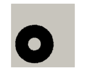
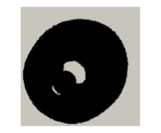
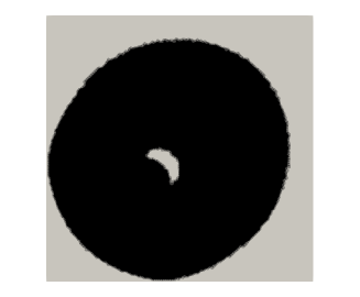
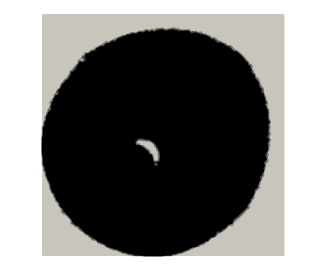
Figure 2: Test 1. The domains $\Omega_{k}$ for k=0, 1, 2, final.

In Figure 1 we show the history of the penalized cost function who has three terms $\mathcal{J}=t_{1}+\frac{1}{\epsilon}t_{2}+\frac{1}{\epsilon}t_{3}$. At the final iteration, we have: $t_{1}=0.825763$, $t_{2}=0.226998$, $t_{3}=0.115119$, $\mathcal{J}_{51}=1.25341$. We recall that $t_{1}$ is the original cost function and $t_{2}$, $t_{3}$ “small” means that the boundary condition (2.2) holds.

The final $y_{h}$, $g_{h}$, $u_{h}$ are presented in Figure 3. The parametrization function $g_{h}:D\rightarrow\mathbb{R}$ is globally continuous, but we observe that it is not smooth enough. In the next test, we also employ a smoothness procedure.

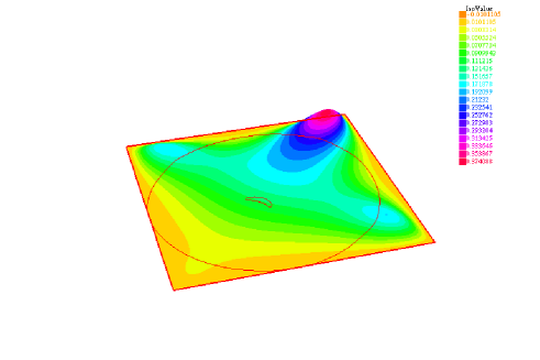
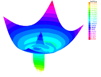
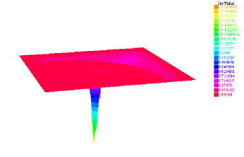
Figure 3: Test 1. Final $y_{h}$ and $\partial\Omega_{h}$ (top). Final $g_{h}$ (left, bottom) and $u_{h}$ (right, bottom).

Test 2.

Case a)

This case is as before, in particular $\epsilon=0.8$, but we change other parameters: the direction $R^{k}$, the triangulation has 9698 vertices and 19034 triangles, $f=0.1$, $\lambda_{0}=0.5$ and $tol=10^{-2}$.

Let $\overline{r}_{h}^{k}$ be the $\mathbb{P}_{3}$ finite elements function associated to the vector $\overline{R}^{k}=R^{q,k}+R^{r,k}+R^{w,k}$, where $R^{q,k}$, $R^{r,k}$ $R^{w,k}$ are obtained using the formulas (4.6), (4.7), (4.14) with $(G^{k},U^{k})$ in place of $(G,U)$. We point out that we use the whole gradient for the descent direction. We have observed that $\overline{r}_{h}^{k}$ is not smooth enough. Then, inspired by [11], we solve the problem: find $\tilde{r}_{h}^{k}\in\mathbb{V}_{h}$, such that

$$\int_{D}\Delta\tilde{r}_{h}^{k}\Delta\varphi_{h}\,d\mathbf{x}=\int_{D}\overline{r}_{h}^{k}\varphi_{h}\,d\mathbf{x},\qquad\forall\varphi_{h}\in\mathbb{V}_{h}$$

and we set $R^{k}$ as the vector associated to $\Pi_{\mathbb{P}_{3}}(\tilde{r}_{h}^{k})$, the $\mathbb{P}_{3}$ projection of $\tilde{r}_{h}^{k}$.

This direction is inspired by the case ii) of Proposition 4.2. If we neglect the effect of interpolation between $\mathbb{P}_{3}$ and the HCT finite element, we have

$$R^{k}=K^{-1}M\overline{R}^{k}=K^{-1}M(R^{q,k}+R^{r,k}+R^{w,k})$$

where $K$, $M$ are two symmetric, positive definite matrices. Using HCT in place of $\mathbb{P}_{3}$ finite element at the regularization stage improves the smoothness of the domain parametrization function $g_{h}$.

The algorithm stops after 155 iterations. We observe in Figure 4 the history of the penalized cost function and in Figure 5 some $\Omega_{k}$. After 155 iterations we have: $t_{1}=0.496559$, $t_{2}=0.289739$, $t_{3}=0.18673$ and $\mathcal{J}_{155}=t_{1}+\frac{1}{\epsilon}t_{2}+\frac{1}{\epsilon}t_{3}=1.09214$.

In Figure 6 we plotted the final $y_{h}$, $g_{h}$, $u_{h}$. This time, $g_{h}$ is smoother than before. The matrices $K^{-1}$ and $M$ operate as filter to improve the smoothness of $\overline{r}_{h}^{k}$. As before, $u_{h}$ is non constant in the exterior of $\Omega_{h}$.

We have also computed the solution of (2.1)-(2.2) for the final domain, see Figure 7.

Figure 4: Test 2, case a). The penalized cost function for iterations $k\geq 4$. The first values are: $\mathcal{J}_{0}=1344.08$, $\mathcal{J}_{1}=724.423$, $\mathcal{J}_{2}=184.156$, $\mathcal{J}_{3}=74.8713$ and the last value is $1.09214$.

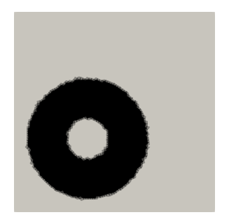
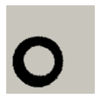
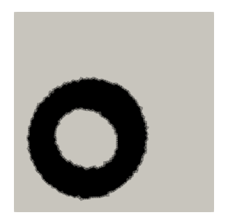
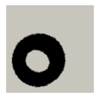
Figure 5: Test 2, case a). The domains $\Omega_{k}$ for k=0, 1, 2, 155.

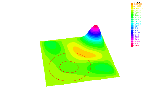
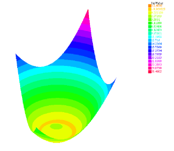
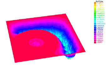
Figure 6: Test 2, case a). Final $y_{h}$ and $\partial\Omega_{h}$ (top). Final $g_{h}$ (left, bottom) and $u_{h}$ (right, bottom).

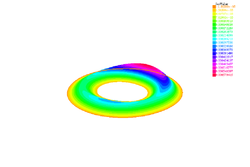
Figure 7: Test 2, case a). Solution of the clamped plate model in the final domain.

Case b)

We use $\epsilon=0.01$, $\lambda_{0}=1$ and the initial domain $\Omega_{0}$, corresponding to $g_{0}(x_{1},x_{2})$ which is maximum of the following functions: $(x_{1})^{2}+(x_{2})^{2}-2.5^{2}$, $-(x_{1}+1)^{2}-(x_{2}+1)^{2}+0.6^{2}$, $-(x_{1}-1)^{2}-(x_{2}+1)^{2}+0.6^{2}$, $-(x_{1}+1)^{2}-(x_{2}-1)^{2}+0.6^{2}$ (the disk of center $(0,0)$ and radius $2.5$ with three circular holes of radius $0.6$). The other values are as in the Test2, case a), in particular the descent direction is given by the whole gradient and we use the same regularization of this direction. Moreover, we normalize the descent direction as follows

$$\left(\frac{\overline{R}^{k}}{\|\overline{R}^{k}\|_{\infty}},\frac{V^{k}}{\|V^{k}\|_{\infty}}\right).$$

The algorithm stops after 25 iterations. The history of the penalized cost function is presented in Figure 8.

We plotted some $\Omega_{k}$ in Figure 9, initially there are 3 holes, at $k=1$ only one hole and finally the domain is simply connected.

In Table 1, we show the terms $t_{1}$, $t_{2}$, $t_{3}$ composing the penalized cost function. We observe that the values on the line $t_{1}$ are decreasing. The terms $t_{2}$, $t_{3}$ concerning the boundary conditions (2.2) are small at the final iteration.

We have computed the solution of (2.1)-(2.2) for the final domain, see Figure 10.

Figure 8: Test 2, case b). The penalized cost function for iterations $k\geq 2$. The first values are: $\mathcal{J}_{0}=257.585$, $\mathcal{J}_{1}=86.8112$ and the last value is $0.544788$.

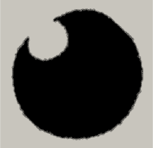
Figure 9: Test 2, case b). The domains $\Omega_{k}$ for $k=0$ (top, left), some intermediate domains during the line-search after $k=0$ ($\lambda=0.8^{8}$, top, middle $\lambda=0.8^{4}$, top, right), $k=1,2,3$ (middle line), $k=10,17,25$ (bottom line).

it.	k=0			k=1	k=2	k=3
$t_{1}$	1.06091	0.90691	0.69644	0.38435	0.12072	0.07963
$t_{2}$	1.89564	1.539	0.99339	0.50898	0.17096	0.14157
$t_{3}$	0.66960	0.57684	0.48017	0.35528	0.19079	0.15602
$\mathcal{J}$	257.585	212.491	148.054	86.8112	36.2963	29.8393

it.	k=10	k=17	k=25
$t_{1}$	0.05954	0.05354	0.05215
$t_{2}$	0.00478	0.00315	0.00182
$t_{3}$	0.01103	0.00514	0.00309
$\mathcal{J}$	1.64094	0.88375	0.54478

Table 1: Test 2, case b). The computed objective function $\mathcal{J}=t_{1}+\frac{1}{\epsilon}t_{2}+\frac{1}{\epsilon}t_{3}$ for the domains as in Figure 9.

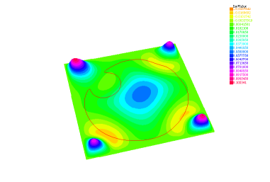
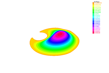
Figure 10: Test 2, case b). Final $y_{h}$ and $\partial\Omega_{h}$ (left) and the solution of the clamped plate model in the final domain (right).

Test 3.

Now, the penalization parameter is $\epsilon=0.1$, $f=0.1$. The initial domain is as in Test 2, case b). The initial guess for the control is $u_{0}=1$ and $tol=10^{-6}$. We use a triangulation of 17175 vertices and 33868 triangles.

For this test, we use a simplified direction $(R^{k},V^{k})$ corresponding to

$$r_{h}^{k}=\sum_{i=1}^{n_{g}}R_{i}^{k}\phi_{i}^{g}=\Pi_{\mathbb{P}_{3}}(-p_{h}u_{h}),\quad v_{h}^{k}=\sum_{i=1}^{n_{u}}V_{i}^{k}\phi_{i}^{u}=\Pi_{\mathbb{P}_{1}}(-p_{h})$$ (5.1)

the $\mathbb{P}_{3}$ interpolation of $-p_{h}u_{h}$ and the $\mathbb{P}_{1}$ interpolation of $-p_{h}$, respectively. It is different from (4.6), but when the quadrature formula employs only the values of functions in the vertices, we have

$$\int_{D}\left(2(g_{h})_{+}u_{h}p_{h}r_{h}^{k}+(g_{h})_{+}^{2}p_{h}v_{h}^{k}\right)d\mathbf{x}=-\int_{D}2(g_{h})_{+}u_{h}p_{h}\Pi_{\mathbb{P}_{3}}(p_{h}u_{h})d\mathbf{x}$$

$$-\int_{D}(g_{h})_{+}^{2}p_{h}\Pi_{\mathbb{P}_{1}}(p_{h})d\mathbf{x}=-\int_{D}2(g_{h})_{+}\left(\Pi_{\mathbb{P}_{3}}(p_{h}u_{h})\right)^{2}d\mathbf{x}-\int_{D}(g_{h})_{+}^{2}\left(\Pi_{\mathbb{P}_{1}}(p_{h})\right)^{2}d\mathbf{x}\leq 0.$$

From (4.5) and the before inequality, we obtain that $\Gamma_{q}$, the terms containing $q$ in (3.17), is negative. In this numerical test, we have also noted that this simplified choice is even a descent direction. There is neither regularization nor normalization of the simplified descent direction. The algorithm stops after 4 iterations. See Figure 11, with the history of the penalized cost function. At the final iteration, we have: $t_{1}=0.287516$, $t_{2}=0.0631412$, $t_{3}=0.047388$ and $\mathcal{J}_{4}=t_{1}+\frac{1}{\epsilon}t_{2}+\frac{1}{\epsilon}t_{3}=1.39281$.

Figure 11: Test 3. The penalized cost function decreases from $26.7086$ to $1.39281$.

We plotted some steps $\Omega_{k}$ in Figure 12 and we note that the topology changes during the iterations.

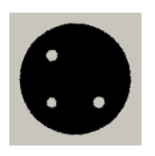
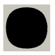
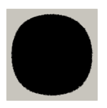
Figure 12: Test 3. The domains $\Omega_{k}$ for $k=0$ (top, left), intermediate domain during the line-search after $k=0$ ($\lambda=0.8^{15}$, top, middle), $k=1$ (top, right), $k=2$ and $k=4$ (bottom).

In Figure 13, we have plotted the final $y_{h},g_{h},u_{h}:D\rightarrow\mathbb{R}$. The initial domain is as for Test 2, case b). The value of the original cost at the initial iteration is a little bit different from Test 2, case b) since the meshes are different.

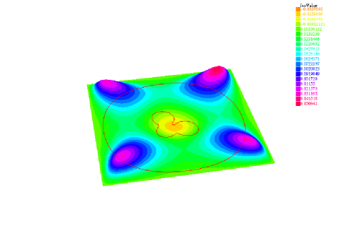
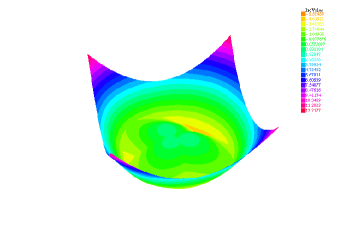
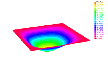
Figure 13: Test 3. Final $y_{h}$ and $\partial\Omega_{h}$ (top). Final $g_{h}$ (left, bottom) and $u_{h}$ (right, bottom).

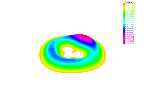
Figure 14: Test 3. Solution of the clamped plate model in the final domain.

References

[1]
R. Adams,
Sobolev spaces, Academic Press, 1975.
[2]
Agmon, S.,
The Lp approach to the Dirichlet problem. I. Regularity theorems.
Ann. Scuola Norm. Sup. Pisa Cl. Sci. (3) 13 (1959), 405-448.
[3]
Alekseev, V.M., Tikhomirov, V.M., Fomin, S.V.,
Optimal control.
Consultants Bureau, Plenum Publishing Corp.
New York, 1987.
[4]
G. Allaire,
Conception optimale de structures,
Volume 58 of Mathématiques & Applications [Mathematics & Applications].
Springer-Verlag, Berlin, 2007.
[5]
Amstutz, S., Andrä, H.,
A new algorithm for topology optimization using a level-set method.
J. Comput. Phys. 216 (2006), no. 2, 573-588.
[6]
Amstutz, S., Bonnafé, A.,
Topological derivatives for a class of quasilinear elliptic equations.
J. Math. Pures Appl. (9) 107 (2017), no. 4, 367-408.
[7]
V. Arnautu, H. Langmach, J. Sprekels, D. Tiba,
On the approximation and optimization of plates,
Numer. Funct. Anal. Optim. 21 (2000) no. 3-4, 337–354.
[8]
Bandle, C.,
Dido’s problem and its impact on modern mathematics.
Notices Amer. Math. Soc. 64 (2017), no. 9, 980-984.
[9]
Bendsoe, M. P.; Sigmund, O.,