The evolution of collision debris near the $\nu_{6}$ secular resonance and its role in the origin of terrestrial water

Abstract

This work presents novel findings that broadens our understanding of the amount of water that can be transported to Earth. The key innovation lies in the combined usage of Smoothed Particle Hydrodynamics (SPH) and $N$-body codes to assess the role of collision fragments in water delivery. We also present a method for generating initial conditions that enables the projectile to impact at the designated location on the target’s surface with the specified velocity. The primary objective of this study is to simulate giant collisions between two Ceres-sized bodies by SPH near the $\nu_{6}$ secular resonance and follow the evolution of the ejected debris by numerical $N$-body code. With our method 6 different initial conditions for the collision were determined and the corresponding impacts were simulated by SPH. Examining the orbital evolution of the debris ejected after collisions, we measured the amount of water delivered to Earth, which is broadly 0.001 ocean equivalents of water, except in one case where one large body transported 7% oceans of water to the planet. Based on this, and taking into account the frequency of collisions, the amount of delivered water varies between 1.2 and 8.3 ocean’s worth of water, depending on the primordial disk mass. According to our results, the prevailing external pollution model effectively accounts for the assumed water content on Earth, whether it’s estimated at 1 or 10 ocean’s worth of water.

1 Introduction

The inner Solar System planets are generally dry (Abe et al., 2000; Raymond & Morbidelli, 2022). However, there is some evidence of water on certain inner rocky planets. Earth is the only planet in the inner Solar System known to have liquid water on its surface. About 70% of Earth’s surface is covered in oceans. All of Earth’s oceans contain roughly $2.5\cdot 10^{-4}\mathrm{M_{\oplus}}$ water, where $\mathrm{M_{\oplus}}$ denotes the mass of the Earth. This amount is often referred to as one ’ocean’ of water, hereafter its mass is denoted by $\mathrm{M_{\mathrm{o}}}$. However, the amount of water in Earth’s interior is much more uncertain, with different studies suggesting vastly different quantities of water trapped in hydrated silicates and other minerals. It is generally assumed that the amount of water in the interior and on the surface of Earth is between 1 and 10 ‘oceans’ (e.g. Abe et al., 2000; Hirschmann, 2006; Marty, 2012).

Overall, studies suggest that the origin of Earth’s water is a complex process that involves the accretion of water from multiple sources over a long period of time. Below, we list these potential sources of water on rocky planets. Cosmochemical tracers such as isotopic ratios, mainly the D/H ratio, may constrain the origin of Earth’s water (for an overview of the D/H measurements, see e.g. Alexander et al., 2012; Morbidelli et al., 2000; Marty, 2006). There are six potential models to explain how water was delivered to Earth. They can broadly be divided into two categories based on whether the sources of water are local or external. The local source models include (a) the adsorption of water vapour onto silicate grains and (b) the oxidation of H-rich primordial envelope. The external source models include (i) the "pebble" snow model, (ii) the wide feeding zone, (iii) the external pollution, and (iv) the inward migration model. For a detailed description of these models see e.g. Raymond & Morbidelli (2022).

According to recent research by Raymond & Morbidelli (2022); Morbidelli et al. (2000), the prevailing theory suggests that the main source of water on Earth is external pollution from the outer regions of the asteroid belt, rather than local sources. It is believed that this water originates from a few planetary embryos located in the outer part of the asteroid belt, as proposed by Morbidelli et al. (2000). According to the external pollution model, the presence of giant planets strongly influences the orbits of the remaining planetesimals, especially during the phase of rapid gas accretion. In the course of this period, the mass of the giant planets can increase rapidly, from $\sim\,10-20\,\mathrm{M_{\oplus}}$ to hundreds of Earth masses on a few $10^{5}$ years timescale. The rapid mass increase excites the orbits of the nearby planetesimals that managed to avoid accretion by the growing giants. A multitude of planetesimals experience close encounters with the growing planet, resulting in scattering in all directions. Bodies that are on elliptical orbits that cross the orbit of the giant planet at apostar distance may experience significant energy loss due to gas drag. As a result, the planetesimal’s farthest point moves inward and the body will not suffer any more close encounters with the proto-Jupiter.

The most significant secular resonance in our solar system is the $\nu_{6}$ resonance (Ito & Malhotra, 2006; Minton & Malhotra, 2011), which has been in the focus of research of resonant dynamics for several decades and thus has an abundant literature. The $\nu_{6}$ secular resonance involves the apsidal precession of asteroids denoted by $g$ and Saturn denoted by $g_{6}$. The resonance condition is defined by $|g-g_{6}|<\delta$, where $g_{6}\approx 28.2455$ arcsec/year (derived from the LONGSTOP 1B numerical integration (Nobili et al., 1989)), and the half-width of the resonant strip, $\delta$, is usually taken as 1 arcsec/yr.

Froeschle & Scholl (1986) conducted numerical integrations over 1 million years to study the orbital evolution in the $\nu_{6}$ at 2.05 au. The results revealed that significant variations in eccentricity led to the presence of direct Earth-crossers originating from this secular resonance. The authors suggest that secular resonances should be considered as potential sources of meteorites. Later on numerical simulations by Scholl & Froeschle (1991) demonstrated that the $\nu_{6}$ secular resonance often in synergy with the 4/1 mean motion resonance with Jupiter, creates a wide region where Earth-crossing chaotic orbits are produced. The 4/1 resonance rapidly increases eccentricity to 0.5 earth-crosser, whereas remaining in the $\nu_{6}$ resonance requires at least several hundred thousand years to become an earth-crosser. The analytical model of Morbidelli & Henrard (1991) is suitable for a global description of dynamics in secular resonances of order 1. The model is applied to investigate the secular resonances $\nu_{6}$, $\nu_{5}$, and $\nu_{16}$, and illustrations of the secular motion are provided. The $\nu_{6}$ resonance sets the inner boundary of the asteroid belt at approximately 2 au. A significant number of near-Earth asteroids originate from the inner main belt rather than the middle or outer belt (Bottke et al., 2002). Many of these asteroids within the inner main belt are affected by the $\nu_{6}$ resonance and eventually acquire Earth-crossing orbits (Morbidelli et al., 1994; Bottke et al., 2000).

In a recent paper by Smallwood et al. (2018) the authors conducted $N$-body simulations of a planetary system with an asteroid belt to study how the architecture of the system affects the asteroid impact rate on Earth. The results revealed the significant role of the $\nu_{6}$ resonance in the frequency of asteroid collisions with Earth. In further investigations, they replaced Earth with a 10 $\mathrm{M_{\oplus}}$ super-Earth and measured how the asteroid collision rate with Earth changes. If the super-Earth orbited beyond 0.7 au, a significant increase in the number of collisions was observed. However, when it orbited between 1 and 1.5 au, the collision rate decreased. Additionally, altering Saturn’s semi-major axis substantially reduced the asteroid collision rate, while increasing its mass raised it.

The formation of the Hungaria family provided further motivation for selecting the location of the collision. The inner edge of the main asteroid belt close to $\nu_{6}$ is home to the Hungaria asteroids, including the Hungaria family, which originated from the catastrophic collision of the (434) Hungaria asteroid (Warner et al., 2009; Forgács-Dajka et al., 2022). This is a direct evidence that collisions occurred in the past within this region.

In a recent paper by Martin & Livio (2021) (hereafter ML) the researchers compared the impact efficiencies of different locations in the asteroid belt, namely the $\nu_{6}$ secular resonance at $a\approx 2.05$ au, at the 2:1 mean-motion resonance with Jupiter at $a\approx 3.32$ au and the outer asteroid belt at $a\approx 4.05$ au, where $a$ denotes the semi-major axis. They estimated the potential amount of water delivered to Earth and found that the majority of asteroids that collided with Earth originate from the $\nu_{6}$ resonance. About 2% of asteroids from $\nu_{6}$ collide with Earth, while the collision probabilities from other resonances are orders of magnitude smaller. If the majority of asteroids in the primordial asteroid belt were displaced to the $\nu_{6}$ secular resonance, e.g. by chaotic diffusion (Kővári et al., 2023), gravitational scattering, gas drag or the Yarkovsky effect, it is possible that up to $\sim 8$ oceans’ worth of water could have been transported to Earth. Thus the delivery of at least 1 $\mathrm{M_{\mathrm{o}}}$ of water from the asteroid belt is possible, but to explain the delivery of 10 $\mathrm{M_{\mathrm{o}}}$ is more challenging.

In this study, we perform an analysis similar to that of ML but specifically focus on tracking the evolution of debris ejected during collisions of large protoplanets. Following the oligarchic growth model proposed by Kokubo & Ida (2000), we assume that the terrestrial planet formation has been almost finished. At this stage, protoplanets in the inner disk may have grown to Ceres size and potentially larger beyond the snowline. The impact of two Ceres-sized bodies occurs near the $\nu_{6}$ secular resonance, where the ejected debris instantly acquires significant eccentricity and inclination. The resonance further increases the eccentricity and inclination of a portion of the debris. As a result, the majority of the debris is rapidly transported to chaotic orbits and can reach the inner planets. The water content of the debris is determined by the original composition of the colliding bodies, and the smoothed particle hydrodynamics (SPH) code consistently accounts for the composition of individual fragments. Thus, in this aspect, we take a step closer to simulating reality. In this study, the simulations of collisions were conducted using the SPH code, which is described in detail in the paper of Schäfer et al. (2020).

In this research, we take a step forward in the simulation of the origin of Earth water. We focus on estimating the amount of water that could have been transported to Earth via collision fragments which were created by a giant impact between two protoplanets. To this end, the dynamical evolution of all fragments will be followed until they impact a large body or the simulation time ends. This scenario is an extension of the external pollution model, since the sudden eccentricity and inclination growth is principally due to collision and not to gravitational interactions. In Section 2, we present the definition of the collision geometry, a short description of the applied SPH and $N$-body simulations and a detailed description of how the initial conditions were constructed from the parameters defining the impact. Section 3 presents the results of the simulations of both the SPH and the $N$-body codes, and we present estimations of how much water could have been transported to the Earth via fragments resulted form a giant collision. We discuss the consequences of water delivery to Earth and draw our conclusions in Section 4.

2 Collision geometry, SPH and $N$-body simulations

In this study the Runge–Kutta–Nystrom 7(6) (RKN) Dormand & Prince (1978) algorithm was utilized with adaptive step size control. The method has an acceptable speed and accuracy in most situations. The integrator was used to model the evolution of a population of asteroids and test particles under the gravitational attraction of Venus, Earth, Mars, Jupiter and Saturn. Uranus and Neptune are not considered in the simulation due to their negligible impact on the dynamics of Jupiter, Saturn and the inner Solar System objects. In the $N$-body code based on the RKN algorithm, all massive bodies interact with all others. Test particles do not influence the motion of the other bodies. In the model we have assumed that all planets have reached their current mass and move on their current orbits. In the simulations, the gas disc had dissipated by this stage and thus gas friction in our simulations is ignored. In the $N$-body simulations, all collisions between bodies are treated as follows: when a close approach with a separation less than the sum of the two radii is detected, the two colliding protoplanets merge to form a new body with a mass equal to the sum of their masses. The orbital elements of the newly formed body are determined based on the position and velocity of the center of mass of the two colliding bodies at the moment of impact. In each collision the composition of the resulting body is determined based on the material composition of the colliding bodies. Most of the previous work on planet formation used this oversimplified treatment of collisions. In the $N$-body runs in order to determine the effect of collisions on the composition of massive bodies, we track the collision history of each individual fragment with mass.

2.1 Initial condition

The process to create collision fragments that originate from impacting bodies with given orbital elements and collision parameters is complex. A description of this procedure is given below and can be divided into the following four main steps:

1. Calculate the radii of the target $R_{\mathrm{t}}$ and the projectile $R_{\mathrm{p}}$ depending on the composition of the objects.

2. Generate the position and velocity vectors for the planets as well as for the projectile and target. Using the specified orbital elements of the target and the collision-defining parameters one has to calculate the initial conditions for projectile. With these initial conditions, the system is integrated backwards in time for approximately $T_{\mathrm{back}}\approx 10^{4}$ seconds.

3. Compute the collision with the SPH code. From the system obtained at the time $t=T_{\mathrm{back}}$, the initial conditions for the SPH code have to be calculated. With these initial conditions defining the barycentric position and velocity of the Sun, the 5 planets, and the target and projectile, the SPH code is used to simulate the collision for a duration of approximately $T_{\mathrm{SPH}}\approx 8\cdot 10^{4}$ seconds. The end state of the SPH run defines the initial state for the next step.

4. Calculate the initial conditions for the $N$-body code from the SPH run’s end state. In this step, it is necessary to identify the cohesive debris fragments, which are bodies composed of one or more SPH particles. Once this is accomplished, their position and velocity vectors must be computed which in conjunction with the data of the major planets constitute the initial conditions for the N-body simulation. The $N$-body simulator is then integrates the system for a duration of $T=10^{6}$ years.

Typically, it takes about 1 million years for these fragments to be transported into Earth-crossing orbits when their eccentricity is directly increased to around $\approx 0.6$ by the resonance (Morbidelli et al., 1994; Smallwood et al., 2018). Below, we provide a detailed description of the above four steps.

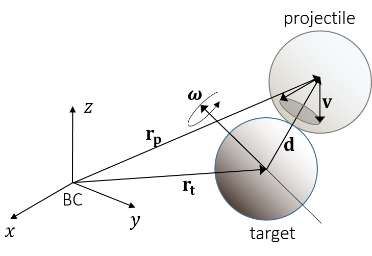
Figure 1: The collision of two bodies in the barycentric coordinate system. The geometry of the collision is defined by the $\mathbf{d}$ relative position and $\mathbf{v}$ relative velocity vectors.

Figure 2: The plane of $\xi^{\prime\prime}-\zeta^{\prime\prime}$ is defined by the $\mathbf{d}$ and $\mathbf{v}$ vectors. The grey-coloured circle denotes the basalt core, while the sky blue denotes the ice mantel.

To complete the first step, we based our assumptions on the observations of Thomas et al. (2005). The authors have analyzed the Ceres’ spectral features in reflected sunlight and demonstrated that the presence of a rocky core and a water-ice mantle aligns with the data assuming the densest materials for the core with a mean density of 2.077 kg m^-3. They estimated that the ice mantles have a thickness ranging from 110 to 124 km, accounting for 24-26% of the total mass of the object. In accordance with these results, in the present paper, the composition of the impacting bodies consists of a basaltic core and a mantle composed of water ice. This structural composition of bodies were utilized by Maindl et al. (2014) when studying the fragmentation of icy objects.

Therefore, our scenarios include two Ceres-mass $M_{\mathrm{Ceres}}=9.38\cdot 10^{20}$ kg protoplanets, where both bodies consist of a basalt core (75% of mass) and a mantle/shell of water ice (25% of mass). The two protoplanets together contain approximately 0.31 $\mathrm{M_{\mathrm{o}}}$ of water. In Fig. 1, we depict the moment of collision between two bodies in the $\mathrm{BC}xyz$ barycentric coordinate system. The target is the larger of the two colliding bodies, and if the masses are equal, then the object with the smaller identifier number becomes the target. The barycentric position vectors of the target and projectile are denoted as $\mathbf{r}_{t}$ and $\mathbf{r}_{p}$, respectively. The relative position vector of the projectile with respect to the center of the target is $\mathbf{d}$, given by $\mathbf{d}=\mathbf{r}_{p}-\mathbf{r}_{t}$, and the relative velocity vector $\mathbf{v}$ is defined as $\mathbf{v}=\mathbf{v}_{p}-\mathbf{v}_{t}$, where $\mathbf{v}_{t}$ and $\mathbf{v}_{p}$ represent the barycentric velocity vectors of the target and projectile, respectively. The $\mathbf{\omega}$ vector corresponds to the angular velocity vector of the target.

In Fig. 2 the two impacting bodies are shown in the plane of the collision defined by the $\mathbf{d}$ and $\mathbf{v}$ vectors. The basalt core is represented by a light grey coloured circle, while the ice mantle is denoted by a sky blue coloured one. The spatial arrangement of the SPH particles composing the target and projectile is governed by a hexagonal lattice structure. This lattice structure was determined based on the given core and shell masses. The radii of the target and the projectile are equal and denoted by $R_{\mathrm{t}}=R_{\mathrm{p}}=4.974\cdot 10^{5}$ m, resulting in a bulk density of $\rho=1.82$ g cm^-3. The radii of the target’s and projectile’s core are equal too and denoted by $R_{\mathrm{t,c}}=R_{\mathrm{p,c}}=3.956\cdot 10^{5}$ m.

To execute the second step, multiple consecutive rotational transformations need to be performed. It is convenient to perform these rotational transformations in the coordinate system fixed to the target’s center denoted as $O_{\mathrm{t}}$. We denote this coordinate system as $O_{\mathrm{t}}\xi\eta\zeta$, where the $O_{\mathrm{t}}\zeta$ axis corresponds to the rotation axis $\mathbf{\omega}$ of the target, and the plane perpendicular to the $O_{\mathrm{t}}\zeta$ axis and passing through the centre is the $\xi-\eta$ plane, see Fig. 3.

The geometry of the collision is completely determined by the impact position vector $\mathbf{d}$ and the velocity vector $\mathbf{v}$ relative to the origin $O_{\mathrm{t}}$. In previous studies, the $\mathbf{d}$ vector is usually not provided, only the collision velocity $v=|\mathbf{v}|$ and the impact angle $\theta$ are given, where $\theta$ is defined as the smaller angle between the vectors $\mathbf{d}$ and $\mathbf{v}$ at the moment of first contact, see Fig. 2. Therefore, only a "collision cone" is defined, with the apex at the centre of the target $O_{\mathrm{t}}$ and the lateral surface composed of possible collision velocity vectors. The impact velocity is given in mutual escape velocity units which is defined as follows (Genda et al., 2012):

$$v_{\mathrm{esc}}=k_{\mathrm{G}}\sqrt{2\frac{m_{\mathrm{t}}+m_{\mathrm{p}}}{R_{\mathrm{t}}+R_{\mathrm{p}}}},$$ (1)

where $m_{\mathrm{t}}$ and $m_{\mathrm{p}}$ denote the mass of the target and projectile, respectively and $k_{\mathrm{G}}$ is the Gaussian constant of gravity.

When $\theta=0^{\circ}$, the collision is referred to as head-on, while $\theta=90^{\circ}$ corresponds to a grazing collision. In terms of geometric shapes, $\theta$ represents the half-angle of the cone. For the sake of generality, in the following discussion, we also take into account the $\mathbf{d}$ vector. Given $\mathbf{r}_{\mathrm{t}}$ and $\mathbf{v}_{\mathrm{t}}$ of the target, as well as the $O_{\mathrm{t}}\zeta$ axis, $\theta$, and $v$, we aim to determine the barycentric position vector $\mathbf{r}_{\mathrm{p}}$ and velocity vector $\mathbf{v}_{\mathrm{p}}$ of the projectile, see Fig. 1. Let us express the components of the $\mathbf{d}$ and $\mathbf{v}$ vectors in the $O_{\mathrm{t}}\xi\eta\zeta$ "targetgraphic" coordinate system

$$\mathbf{d}=d\left(\begin{array}[]{r}\cos\lambda_{1}\cos\phi_{1}\\ \sin\lambda_{1}\cos\phi_{1}\\ \sin\phi_{1}\end{array}\right),\quad\mathbf{v}=v\left(\begin{array}[]{r}\cos\lambda_{2}\cos\phi_{2}\\ \sin\lambda_{2}\cos\phi_{2}\\ \sin\phi_{2}\end{array}\right)$$ (2)

where $\lambda_{1}$ is the longitude and $\phi_{1}$ is the latitude of vector $\mathbf{d}$, and similarly $\lambda_{2}$ is the longitude and $\phi_{2}$ is the latitude of vector $\mathbf{v}$ (since $\mathbf{v}$ is a free vector, thus we have imaginarily shifted it to the origin $O_{\mathrm{t}}$).

Let $\mathbf{f^{(1)}}$ and $\mathbf{f^{(2)}}$ denote the unit vectors in the directions of $\mathbf{d}$ and $\mathbf{v}$, respectively

$$\mathbf{f}^{(1)}=\frac{\mathbf{d}}{d},\quad\mathbf{f}^{(2)}=\frac{\mathbf{v}}{v}.$$ (3)

Rotate the $O_{\mathrm{t}}\xi\eta\zeta$ coordinate system around the $O_{\mathrm{t}}\zeta$ axis with $\lambda_{1}$ angle and then the resulting the $O_{\mathrm{t}}\xi^{\prime}\eta^{\prime}\zeta^{\prime}$ coordinate system around the $O_{\mathrm{t}}\eta^{\prime}$ axis with $\phi_{1}$. Let us denote the rotation matrix around axis $O_{\mathrm{t}}\zeta$ by $\mathbf{R}_{\mathrm{\zeta}}(\lambda_{1})$, and around the $O_{\mathrm{t}}\eta^{\prime}$ axis by $\mathbf{R}_{\mathrm{\eta^{\prime}}}(\phi_{1})$. They are defined as

$$\mathbf{R}_{\mathrm{\zeta}}(\lambda_{1})=\left(\begin{array}[]{rrr}\cos\lambda_{1}&\sin\lambda_{1}&0\\ -\sin\lambda_{1}&\cos\lambda_{1}&0\\ 0&0&1\end{array}\right),$$ (7)

$$\mathbf{R}_{\mathrm{\eta^{\prime}}}(\phi_{1})=\left(\begin{array}[]{rrr}\cos\phi_{1}&0&\sin\phi_{1}\\ 0&1&0\\ -\sin\phi_{1}&0&\cos\phi_{1}\end{array}\right).$$ (11)

The rotated system is shown in Fig 4, denoted by $O_{\mathrm{t}}\xi^{\prime\prime}\eta^{\prime\prime}\zeta^{\prime\prime}$. The intersection of the collision cone and the $O_{\mathrm{t}}\xi^{\prime\prime}\zeta^{\prime\prime}$ plane specifies a possible collision vector, which we denoted as $\mathbf{\tilde{v}}$ in Fig. 4. An $\alpha$-angle rotation about the $O_{\mathrm{t}}\xi^{\prime\prime}$ axis connects the original $\mathbf{v}$ and $\mathbf{\tilde{v}}$. Then if we denote by $\mathbf{\tilde{f}^{(2)}}$ the unit vector in the direction of $\mathbf{\tilde{v}}$:

$$\mathbf{\tilde{f}^{(2)}}=\frac{\mathbf{\tilde{v}}}{\tilde{v}}=\left(\begin{array}[]{r}-\cos\theta\\ 0\\ \sin\theta\end{array}\right)$$ (12)

and then rotate it around the axis $O_{\mathrm{t}}\xi^{\prime\prime}$ by $\alpha$ it yields

$$\mathbf{{f}^{(2)}}=\left(\begin{array}[]{rrr}1&0&0\\ 0&\cos\alpha&-\sin\alpha\\ 0&\sin\alpha&\cos\alpha\end{array}\right)\mathbf{\tilde{f}^{(2)}}=\left(\begin{array}[]{r}-\cos\theta\\ -\sin\alpha\sin\theta\\ \cos\alpha\sin\theta\end{array}\right).$$ (13)

Let us transform $\mathbf{f}^{(2)}$ back to the original $O_{\mathrm{t}}\xi\eta\zeta$ coordinate system. Applying $\mathbf{R}_{\mathrm{\eta^{\prime}}}(-\phi_{1})$ and then $\mathbf{R}_{\mathrm{\zeta}}(-\lambda_{1})$, we get

$$\mathbf{v}=v\left(\begin{array}[]{rrr}\cos\lambda_{1}\cos\phi_{1}&-\sin\lambda_{1}&-\cos\lambda_{1}\sin\phi_{1}\\ \sin\lambda_{1}\cos\phi_{1}&\cos\lambda_{1}&-\sin\lambda_{1}\sin\phi_{1}\\ \sin\phi_{1}&0&\cos\phi_{1}\end{array}\right)\left(\begin{array}[]{r}f^{(2)}_{x}\\ f^{(2)}_{y}\\ f^{(2)}_{z}\end{array}\right),$$ (14)

where the components of $\mathbf{{f}^{(2)}}$ are given in Eq. (13).

Figure 3: The $O_{\mathrm{t}}\xi\eta\zeta$ targetgraphic coordinate system, where $\mathbf{\omega}$ is the angular velocity of the target, $\lambda$ denotes the longitude and $\phi$ the latitude, $\mathbf{d}$ is the position vector of the projectile, $\mathbf{v}$ is the impact velocity vector. The $\mathbf{d}$ and $\mathbf{v}$ vectors determine the plane of collision, $\theta$ is the impact angle.

Figure 4: The projection of the collision cone onto the plane $O_{\mathrm{t}}\xi^{\prime\prime}\zeta^{\prime\prime}$. The $\mathbf{\tilde{v}}$ is a possible impact vector with the right magnitude $v$ and collision angle $\theta$, which is the half-angle of the cone.

As a last step, one has to transform the vectors into the inertial barycentric coordinate system $\mathrm{BC}xyz$ as shown in Fig. 1. The connection between $\mathrm{BC}xyz$ and $O_{\mathrm{t}}\xi\eta\zeta$ systems is defined by the $\mathbf{\omega}$ angular velocity vector of the target. The components of $\mathbf{\omega}$ in the $\mathrm{BC}xyz$ coordinate system may be given as

$$\mathbf{\omega}=\omega\left(\begin{array}[]{r}\cos\lambda\cos\phi\\ \sin\lambda\cos\phi\\ \sin\phi\end{array}\right),$$ (15)

where $\lambda$ is the longitude and $\phi$ is the latitude in the "barygraphic" coordinate system. The transformation is defined by two subsequent rotations by applying $\mathbf{R}_{\mathrm{x}}(-\lambda)$ and then $\mathbf{R}_{\mathrm{y^{\prime}}}(-\phi)$. The computation of these matrices is similarly done as before.

After performing the aforementioned transformations, we obtain the barycentric coordinates and velocities of the projectile. From these, one can calculate the orbital elements associated with the given collision. These computed orbital elements together with the those of the other bodies are listed in Table 1 for all scenarios and serve as the initial conditions for the backward integration. For all the scenarios the initial orbital elements of the bodies are the same except for the projectile, which are given in the table for all the six scenarios.

According to the last objective in step 2, the backward integration is performed for $T_{\mathrm{back}}\approx 10^{4}$ seconds. As a result, the separation between the colliding bodies will be at least 5 times the sum of their radii. The SPH code requires this initial separation distance in order for the SPH particles to arrange themselves properly due to mutual tidal and gravitational forces. The end state of this backward simulation is used to generate the initial condition for the SPH code. In this article, for simplicity, we assume that initially neither the target nor the projectile rotates around its axis, and that the collision occurs in a plane parallel to the $\mathrm{BC}xy$ plane, thus $\lambda_{1}=0$ and $\phi_{1}=0$ therefore $\mathbf{d}=(d,0,0)$.

Sim.	$v[v_{\mathrm{esc}}]$	$\theta$ [deg]	Body	$m\,[\mathrm{M_{\oplus}}]$	$a$ [au]	$e$	$i$ [rad]	$\omega$ [rad]	$\Omega$ [rad]	$M$ [rad]
			Venus	2.44757e-06	0.72332	6.76124e-3	5.92446e-2	0.95363	1.33761	0.6327
			Earth	3.00244e-06	0.99994	1.70615e-2	4.94382e-5	4.61622	3.47543	2.17442
			Mars	3.22611e-07	1.52358	9.34559e-2	3.22607e-2	5.00092	0.86416	1.36914
			Jupiter	9.54296e-04	5.20147	4.89592e-2	2.27578e-2	4.77563	1.75444	2.20341
			Saturn	2.85725e-04	9.55384	5.37045e-2	4.33936e-2	5.93821	1.98306	2.50830
			Target	4.71882e-10	2.08000	5.00000e-2	8.72664e-2	0	0	0
run1	3.0	30	Projectile	4.71882e-10	2.10526	8.55781e-2	1.21687e-1	0.83226	0	5.57213
run2	3.0	45	Projectile	4.71882e-10	2.11117	8.03866e-2	1.35865e-1	0.69963	0	5.68244
run3	5.0	30	Projectile	4.71882e-10	2.13530	1.23688e-1	1.44479e-1	1.02614	0	5.45849
run4	5.0	45	Projectile	4.71882e-10	2.14546	1.12679e-1	1.67923e-1	0.87794	0	5.56950
run5	7.0	30	Projectile	4.71882e-10	2.17693	1.65018e-1	1.67121e-1	1.12143	0	5.44273
run6	7.0	45	Projectile	4.71882e-10	2.19173	1.48589e-1	1.99636e-1	0.96437	0	5.54775

Table 1: Initial conditions for the $N$-body simulation scenarios for backward integration. The first column contains the name of the simulation. Columns 2 and 3 show the impact velocity $v$ and angle $\theta$, respectively. Column 4 displays the name of the body, Column 5 represents its mass in Earth-mass units. Columns 6-11 show the orbital elements of the bodies, $a$ is the semi-major axis in au, $e$ is the eccentricity, $i$ is the inclination, $\omega$ is the argument of pericenter, $\Omega$ is the longitude of the ascending node, and $M$ is the mean anomaly. The orbital elements of planets listed above the double line are the same for all six runs.

In step 3, the SPH code developed by Schäfer et al. (2020) was utilized. This code has proven to be highly effective in simulating high-resolution surface impacts (Maindl & Haghighipour, 2014; Maindl et al., 2015) as well as investigating collisions between planetesimals and protoplanets (Maindl et al., 2014; Maindl & Dvorak, 2014). It has been successfully utilized in both scenarios, yielding valuable insights and accurate results. In SPH-based simulations, continuous bodies are represented by discrete SPH particles (e.g. Gingold & Monaghan, 1977; Benz & Asphaug, 1995; Maindl et al., 2013; Schäfer, 2005). These particles carry the specific physical properties of interest and contribute to the overall physical properties of their respective volume elements. In this study, we employ a relatively low resolution of $N_{\mathrm{SPH}}\approx 20\cdot 10^{3}$ SPH particles, which means that each SPH particle has a mass of $m_{\mathrm{SPH}}=M_{\mathrm{t}}/N_{\mathrm{SPH}}=4.695\cdot 10^{16}$ kg.

Due to a collision, a large amount of debris is generated and scattered. If we were to consider every debris as a massive body in the $N$-body code, the simulation would take a very long time to run. In order to strike a balance between the statistically significant number of bodies and the runtime of the simulation, we only considered debris with masses denoted as $m_{\mathrm{frag}}$ above a certain threshold as massive bodies and treated the rest as test particles. A fragment is considered as protoplanet if $m_{\mathrm{frag}}\in[10^{-10},10^{-7}]\,\mathrm{M_{\oplus}}$, if $m_{\mathrm{frag}}\in[10^{-13},10^{-10})\,\mathrm{M_{\oplus}}$ then it was treated as planetesimal, and any remaining mass below $10^{-13}\,\mathrm{M_{\oplus}}=1.87\cdot 10^{17}$ kg as test particle. This lower mass limit corresponds to approximately 4 SPH particles. This compromise ensures to get statistically meaningful results and to keep the number of massive bodies manageable while guaranteeing that the debris is not only present in the form of test particles in the $N$-body simulator.

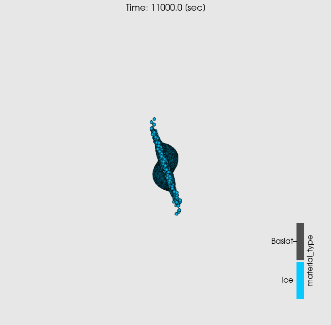
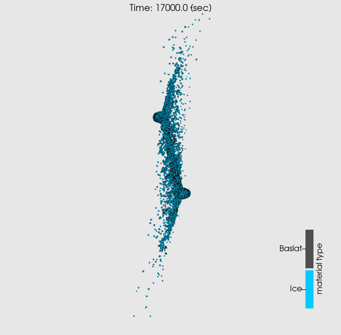
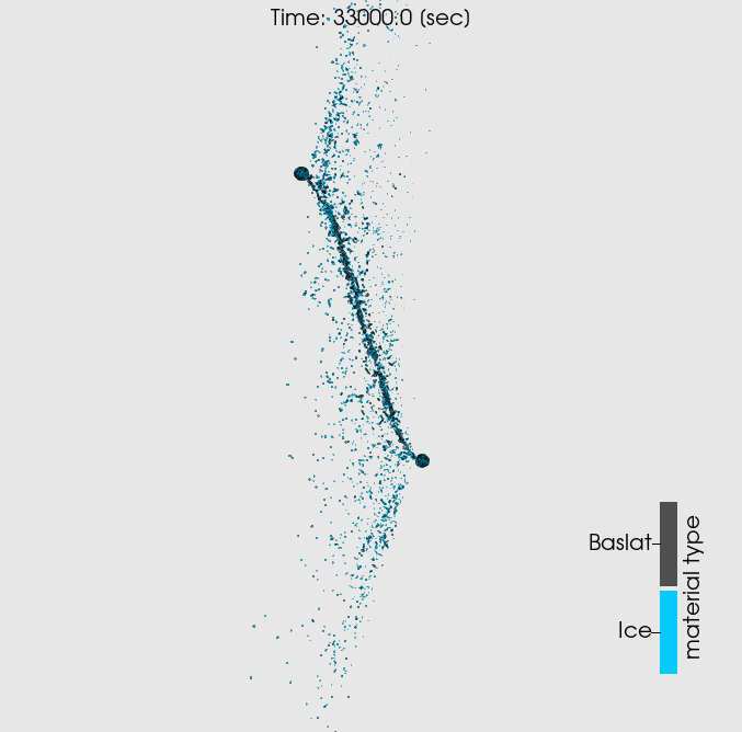
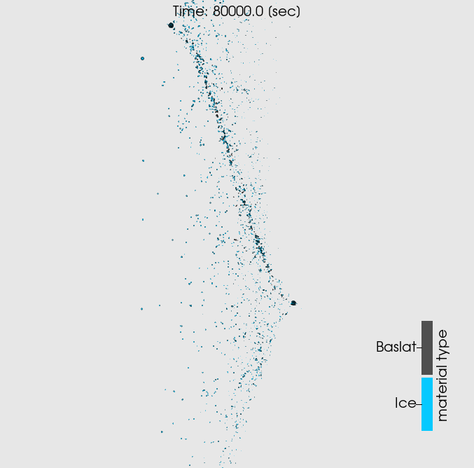
Figure 5: Collision snapshots for $v=3.0\,[v_{\mathrm{esc}}]$ and $\theta=30^{\circ}$. The simulation time for each frame is indicated at the top. The actual collision takes place at $t\approx 10^{4}$ seconds. Basalt material is represented in grey, while water ice is depicted in sky blue. Both bodies have a layer of water ice (25 percent of its total mass). We note that the scale increases on successive snapshots. In the top left panel, it is a few times $\sim 10^{3}$ km, while in the bottom right panel, it is a few times $\sim 10^{5}$ km kilometers.

In Fig. 5, a series of four snapshots are presented for the collision with $\theta=30^{\circ}$ and $v=3.0\,[v_{\mathrm{esc}}]$. The spherical objects are composed of basaltic rock represented by grey and water ice represented by sky blue. Neither of the bodies is rotating at the start of the simulation. The collision happens at $t\approx 10^{4}$ seconds, and the evolution of the colliding bodies is followed via the SPH code for $t=8\cdot 10^{4}$ seconds. The lower right frame in Fig. 5 illustrates the final outcome of the SPH simulation, which will serve as the input for the subsequent $N$-body simulation. The region occupied by the fragments in the final snapshot is $x\in[1.981,\,1.982]$ au, $y\in[8.638,\,10.61]\times 10^{-3}$ and $z\in[-4.737,\,182.6]\times 10^{-5}$ au, which fits in a rectangular cuboid with sizes of $\Delta x=10^{-3},\,\Delta y=2\cdot 10^{-3}$, and $\Delta z=2\cdot 10^{-3}$ au.

From the barycentric position and velocity vectors of the fragments at $t=8\cdot 10^{4}$ seconds, the orbital elements were computed and the eccentricities $e$ and inclinations $i$ versus the semi-major axis $a$ are plotted in Figs. 6 and 7, respectively for all six runs. The large black plus sign indicates the location of the collision at $a=2.08$ au, $e=0.05$, and $i=5^{\circ}$ (the values of the other orbital elements were set to zero, c.f. the data for the Target in Table 1). The blue-filled circles denote the protoplanets, the smaller red circles are the planetesimals, while the small grey dots are the test particles.

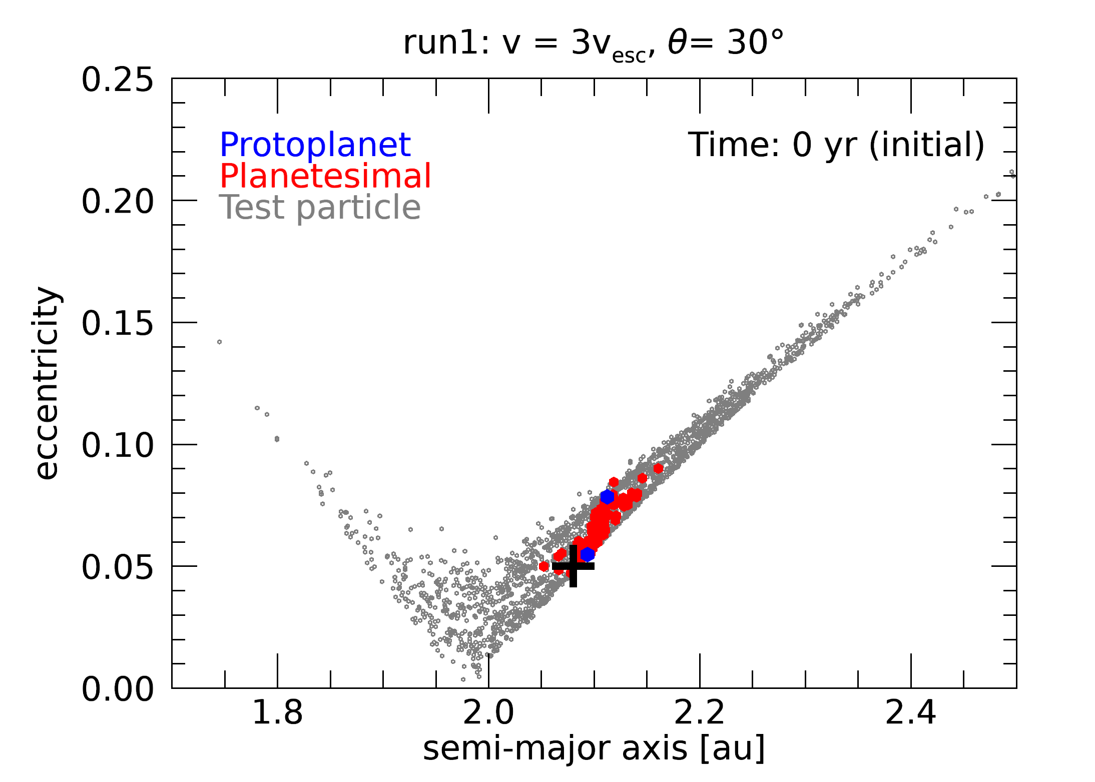
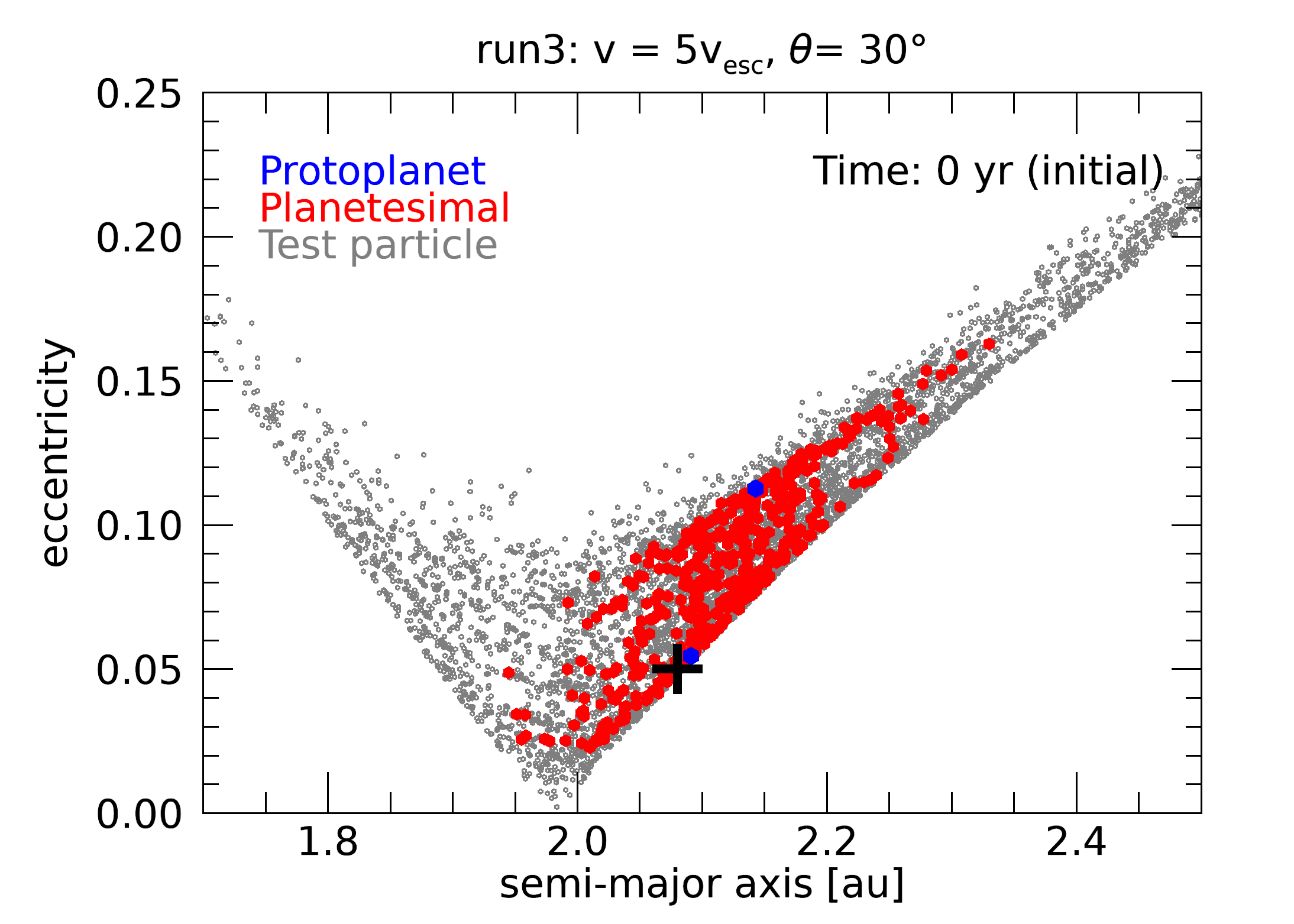
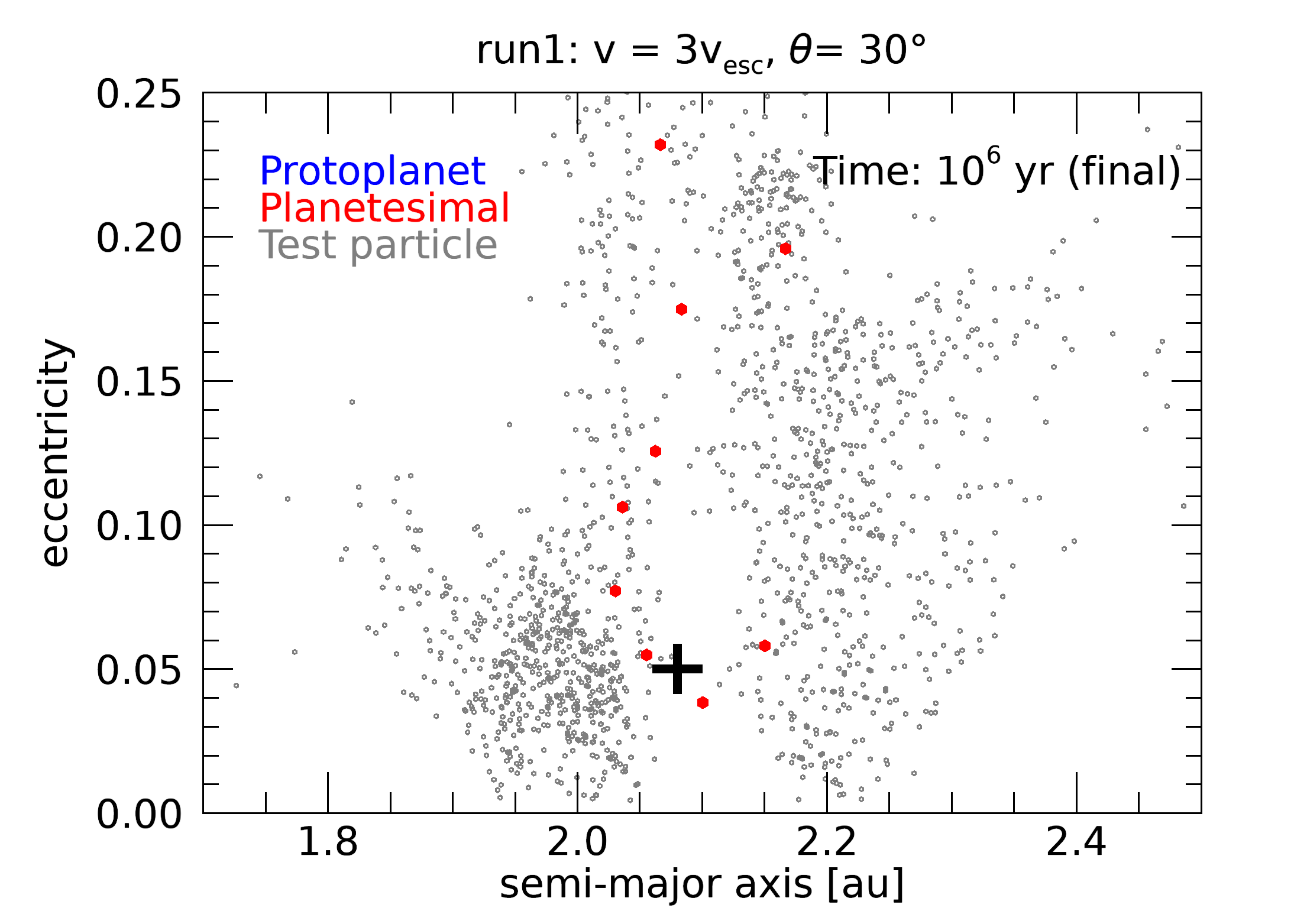
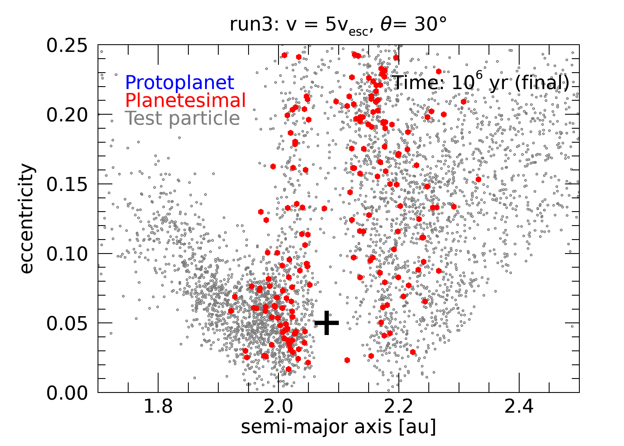
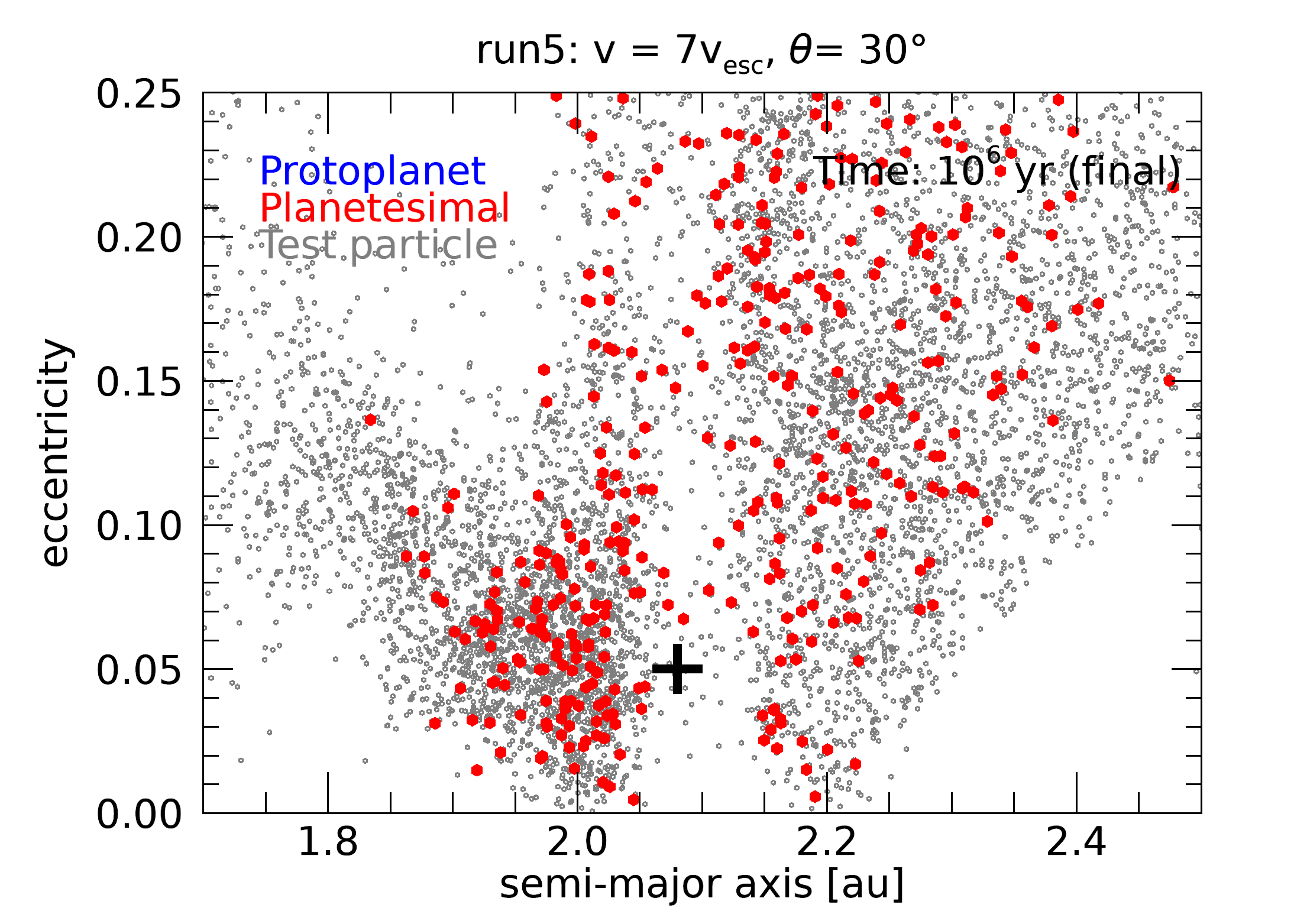
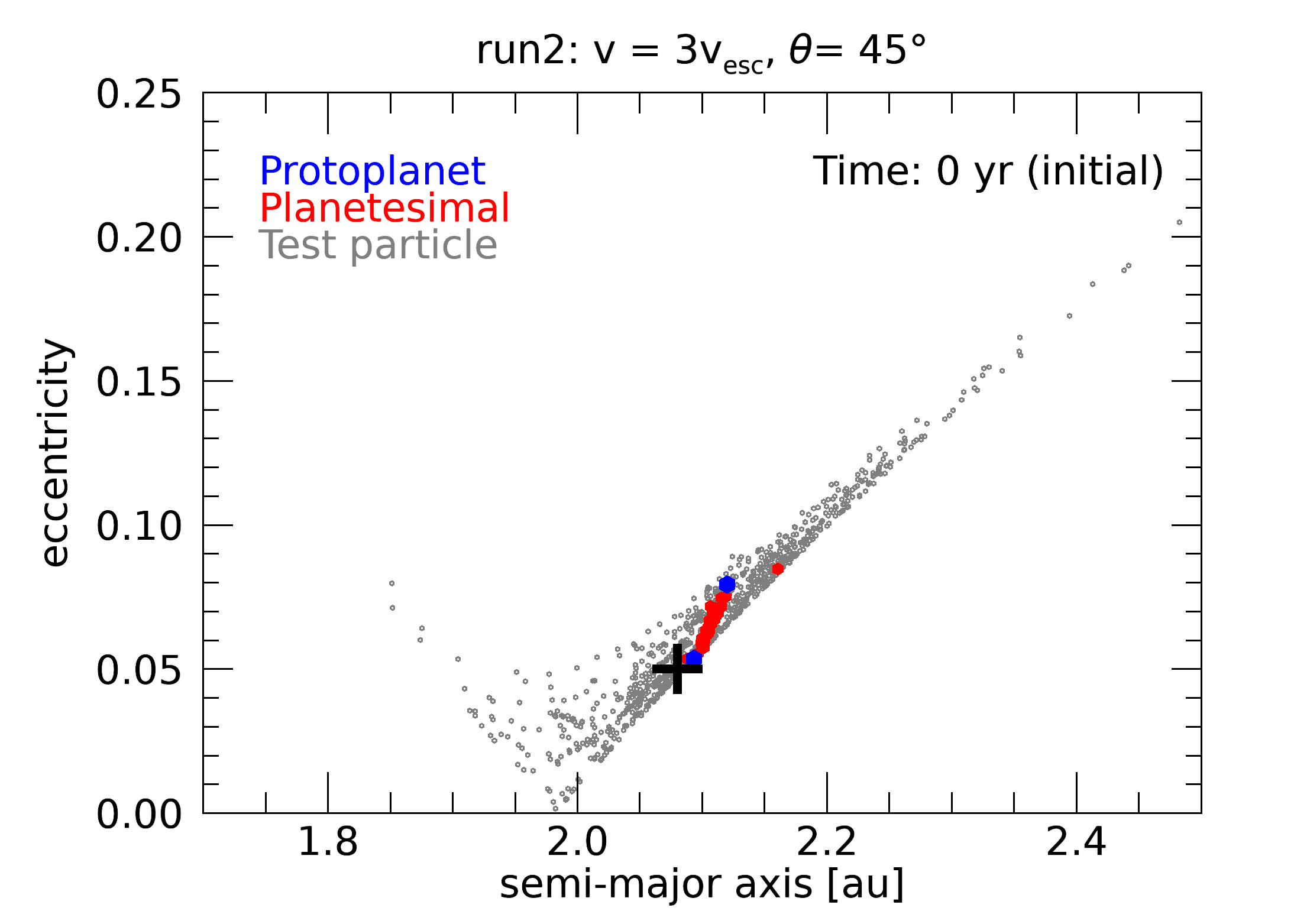
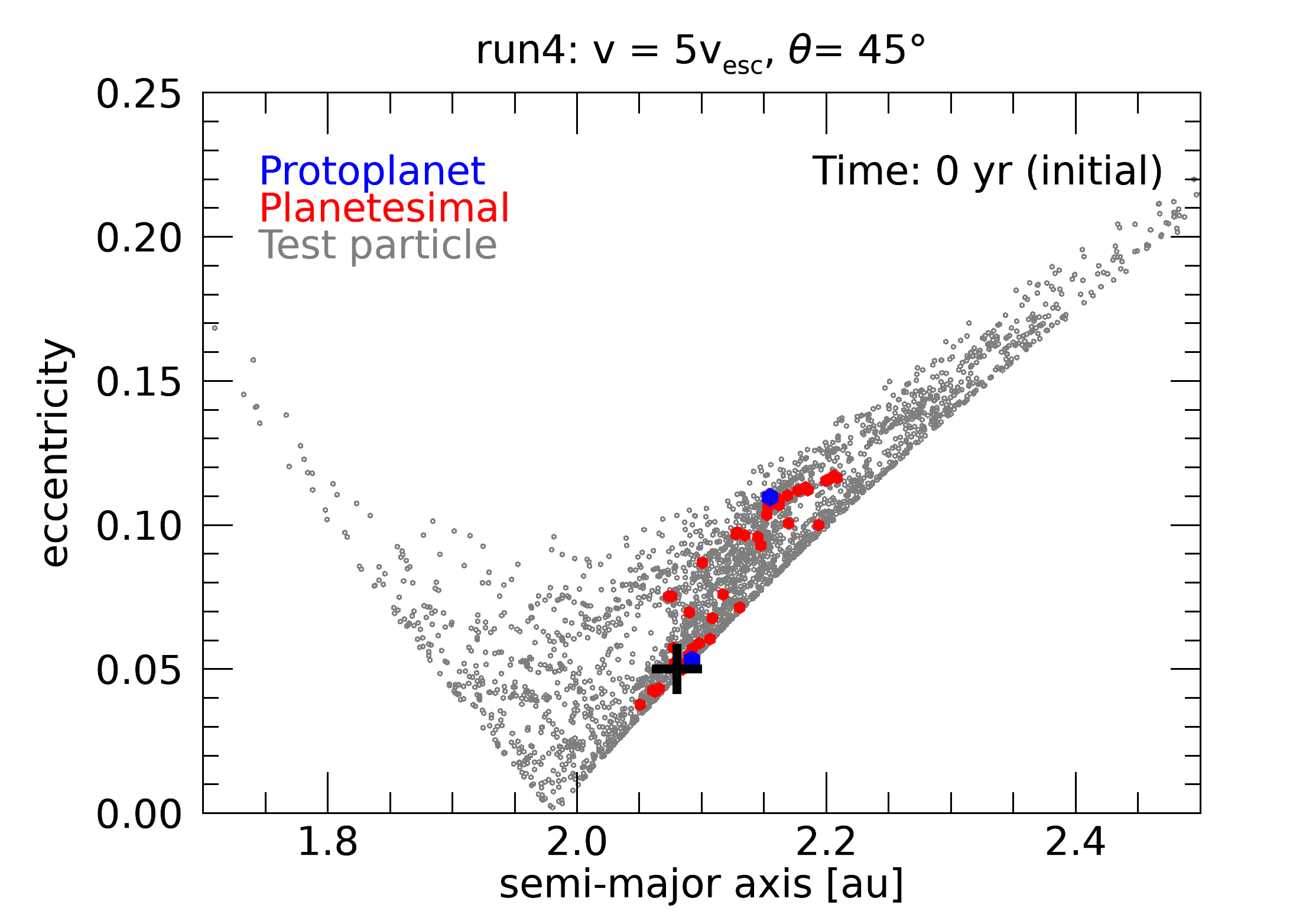
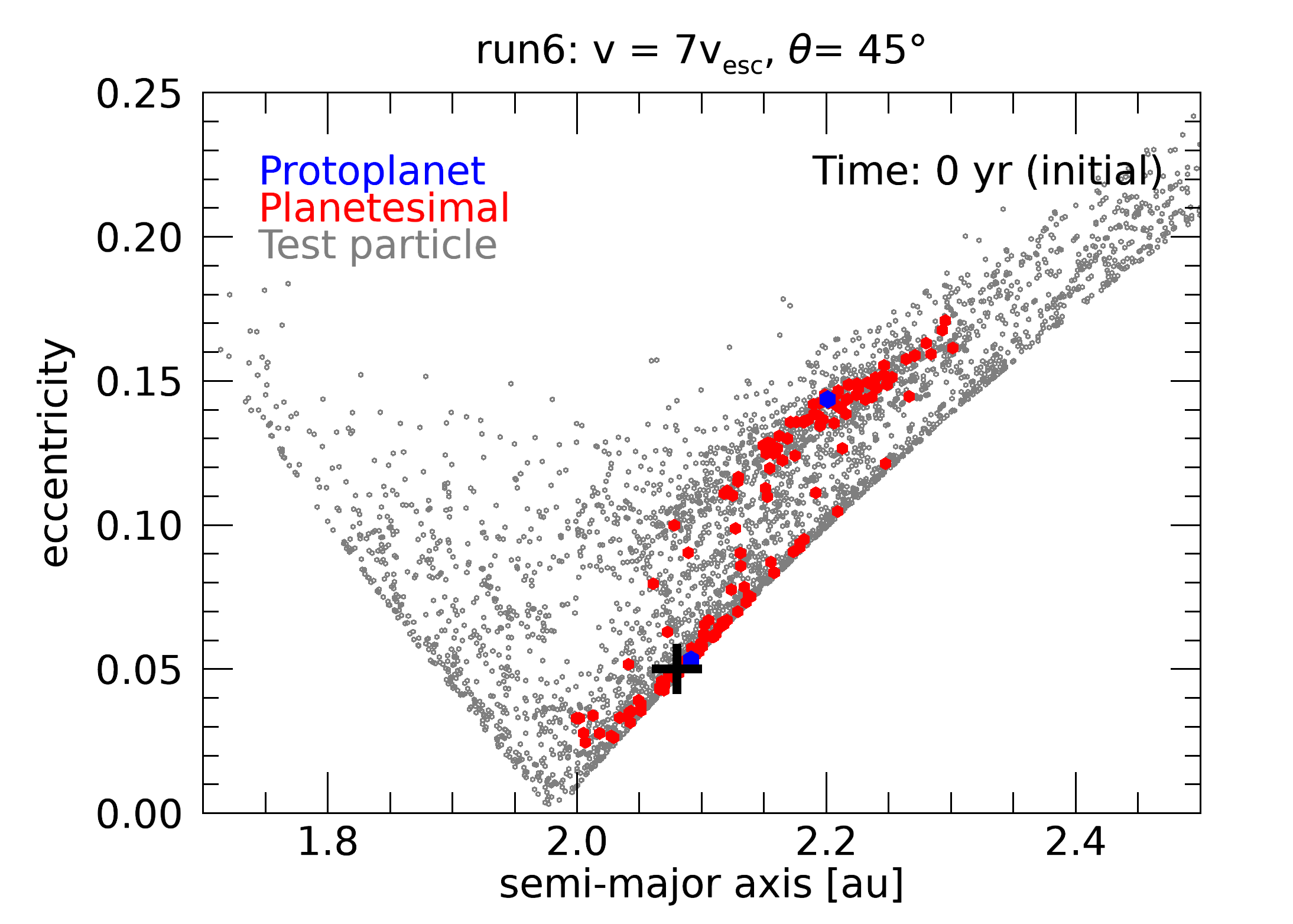
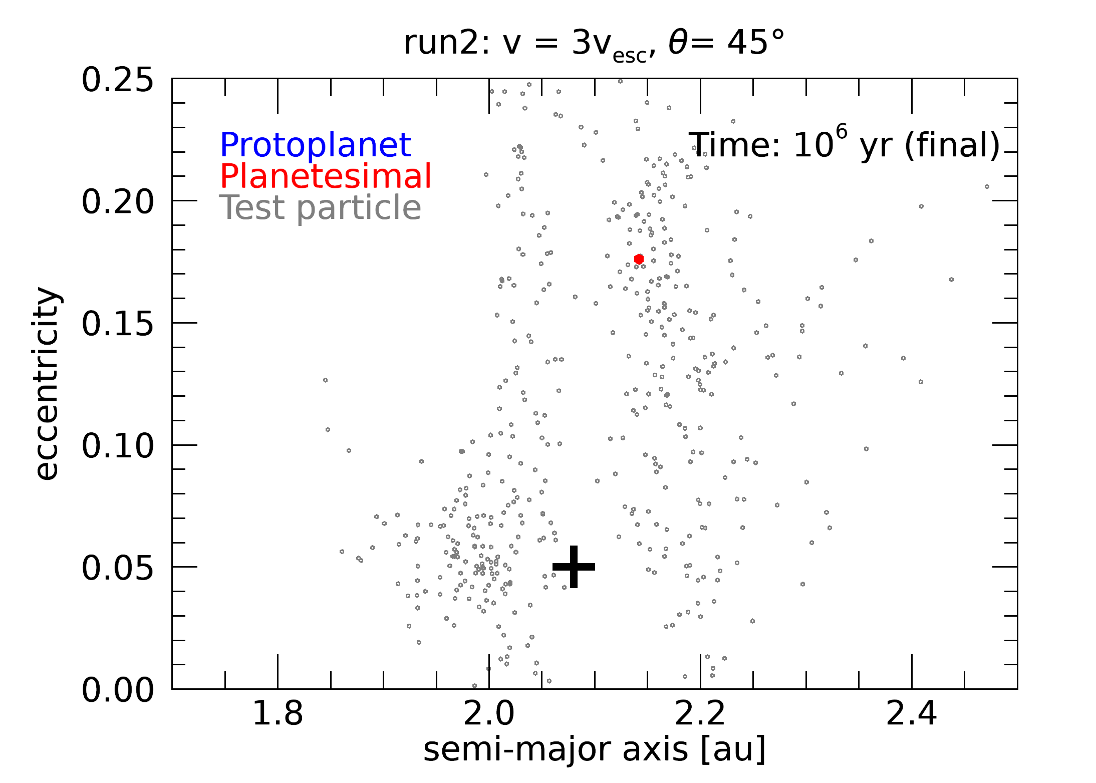
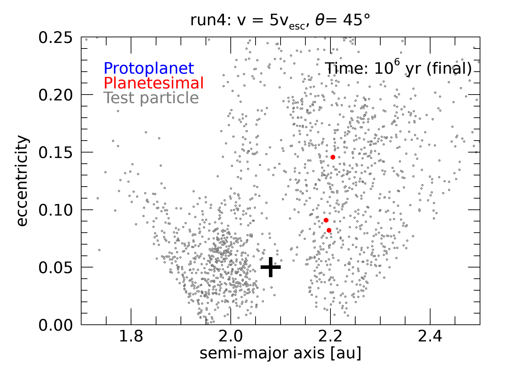
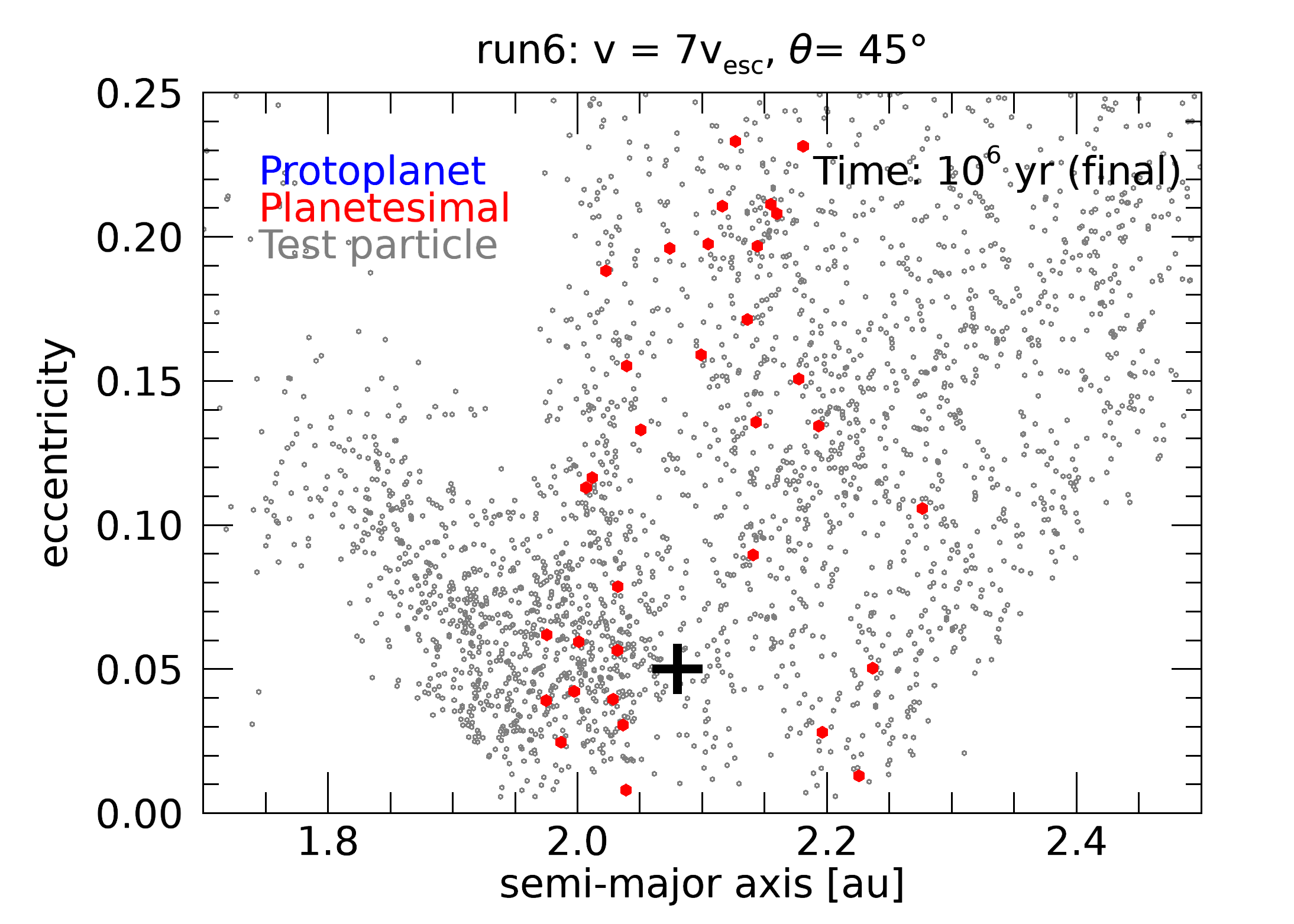
Figure 6: The ($a-e$) plane of the fragments in the $N$-body simulations. The top two rows show the initial (first row) and final (second row) eccentricities of the fragments with $\theta=30^{\circ}$ for different impact velocities, while the third and fourth rows for $\theta=45^{\circ}$ (see Table 2). The initial eccentricities were computed using the barycentric position and velocity vectors taken from the last frame of the SPH simulation (see Fig. 5). The big black plus denotes the position of the impact. Blue circles represent protoplanets, red ones planetesimals while grey dots correspond to test particles.

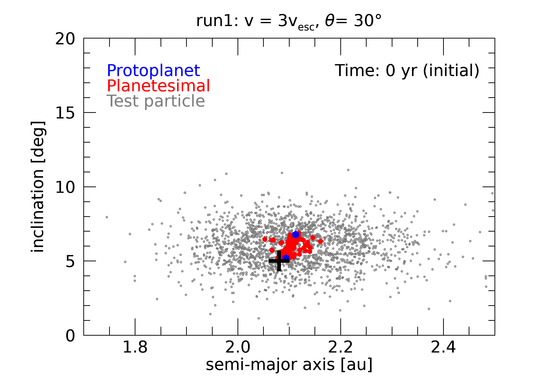
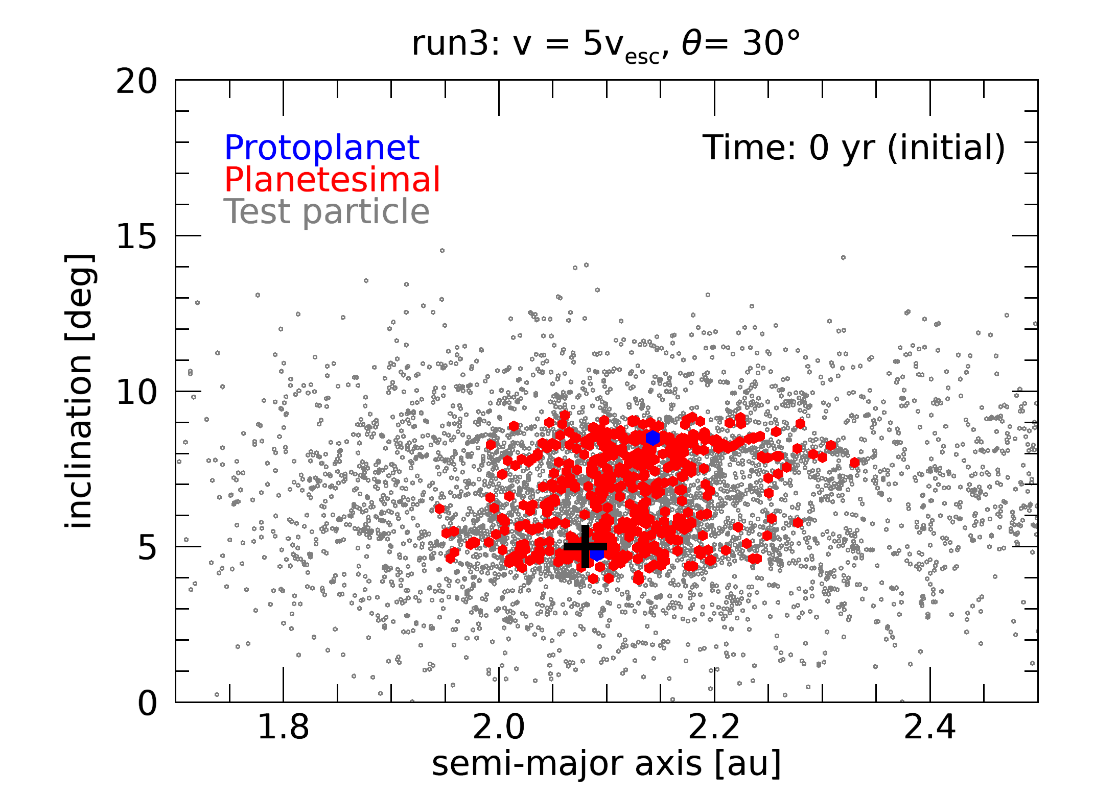
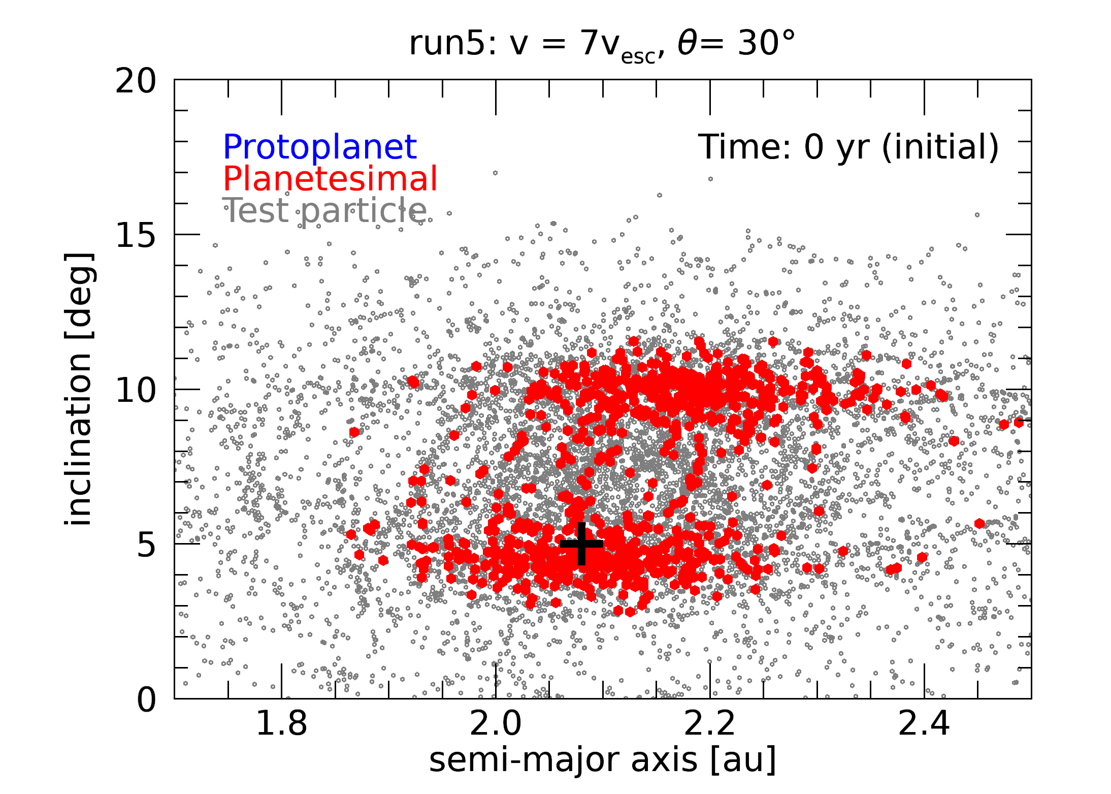
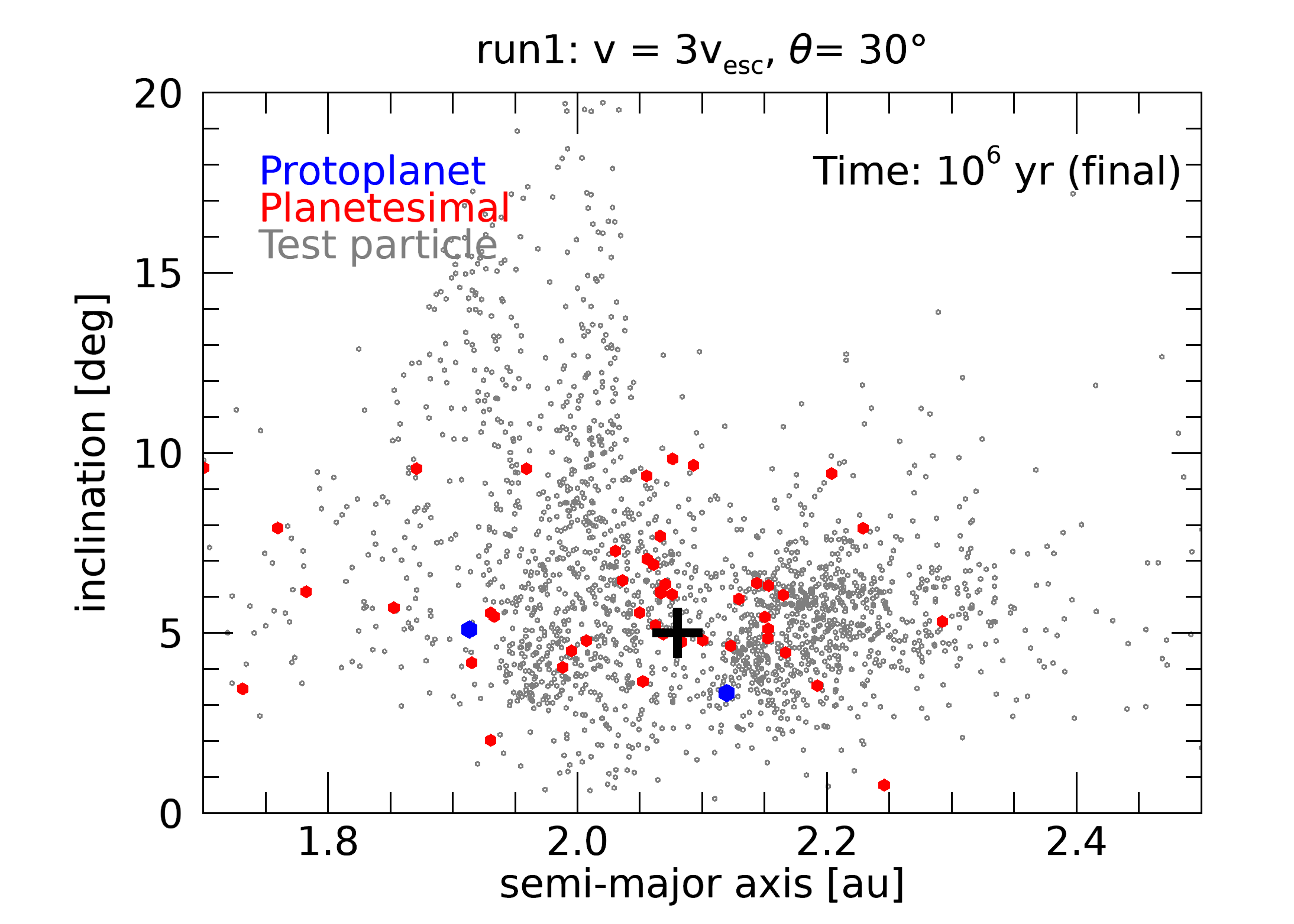
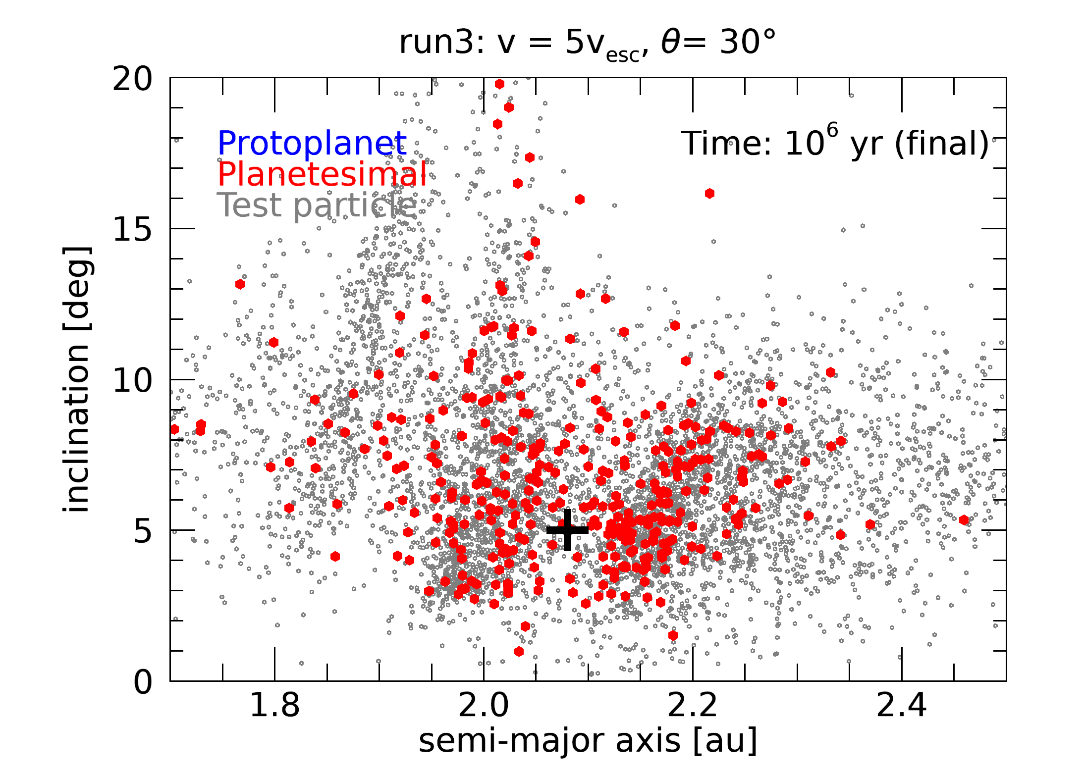
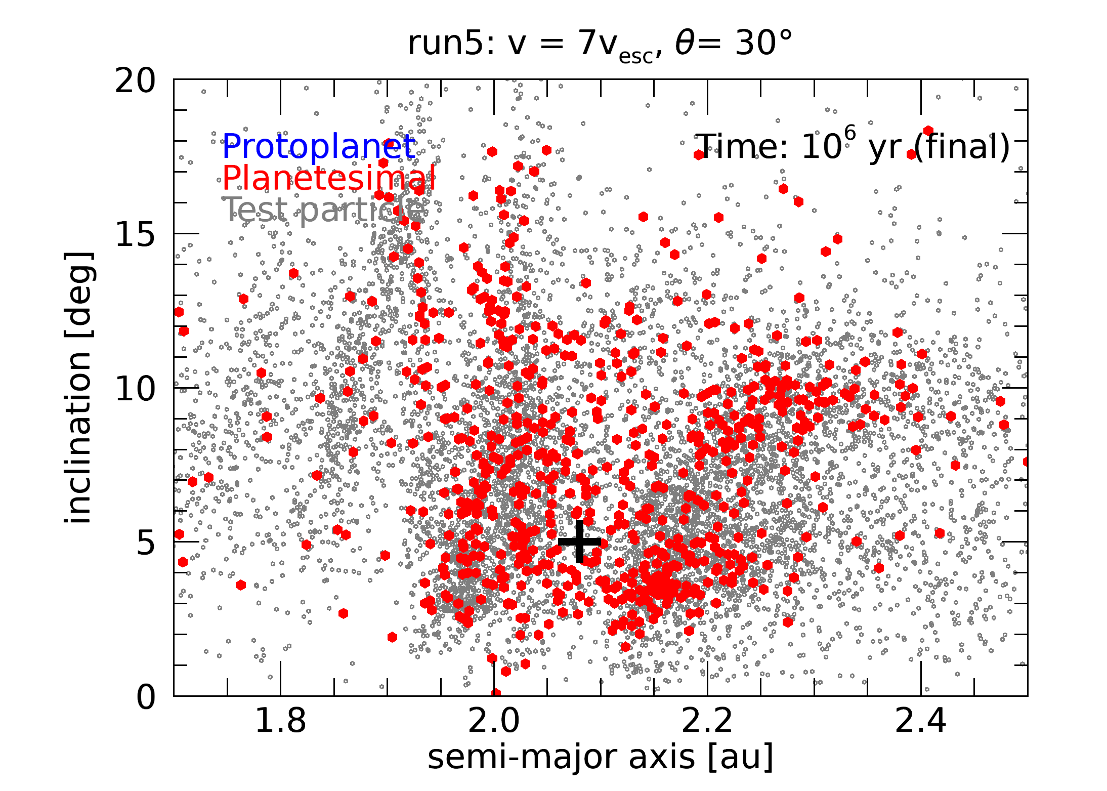
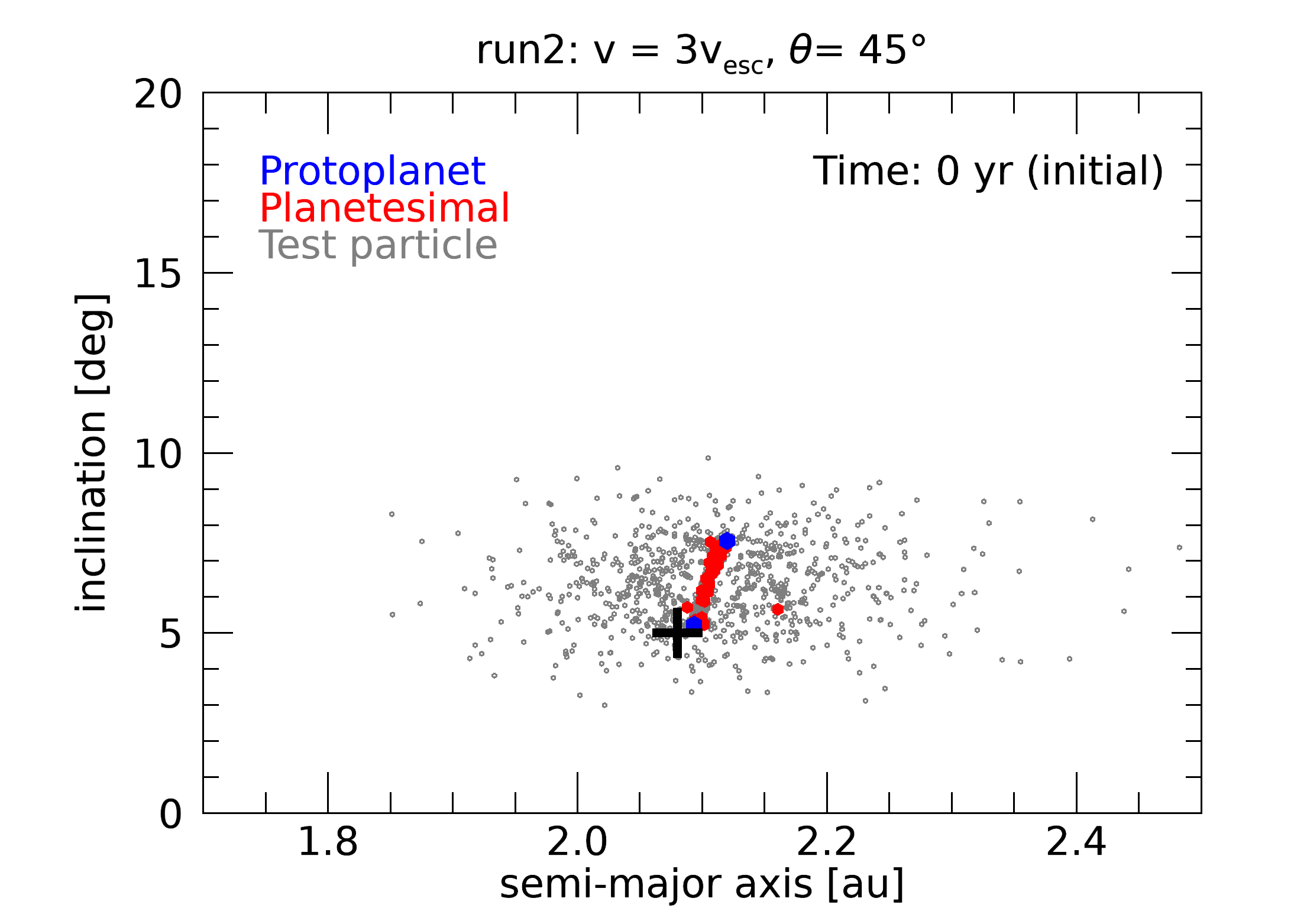
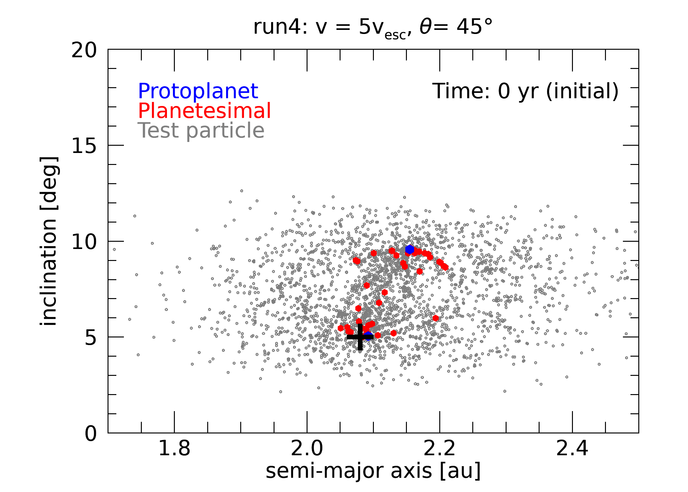
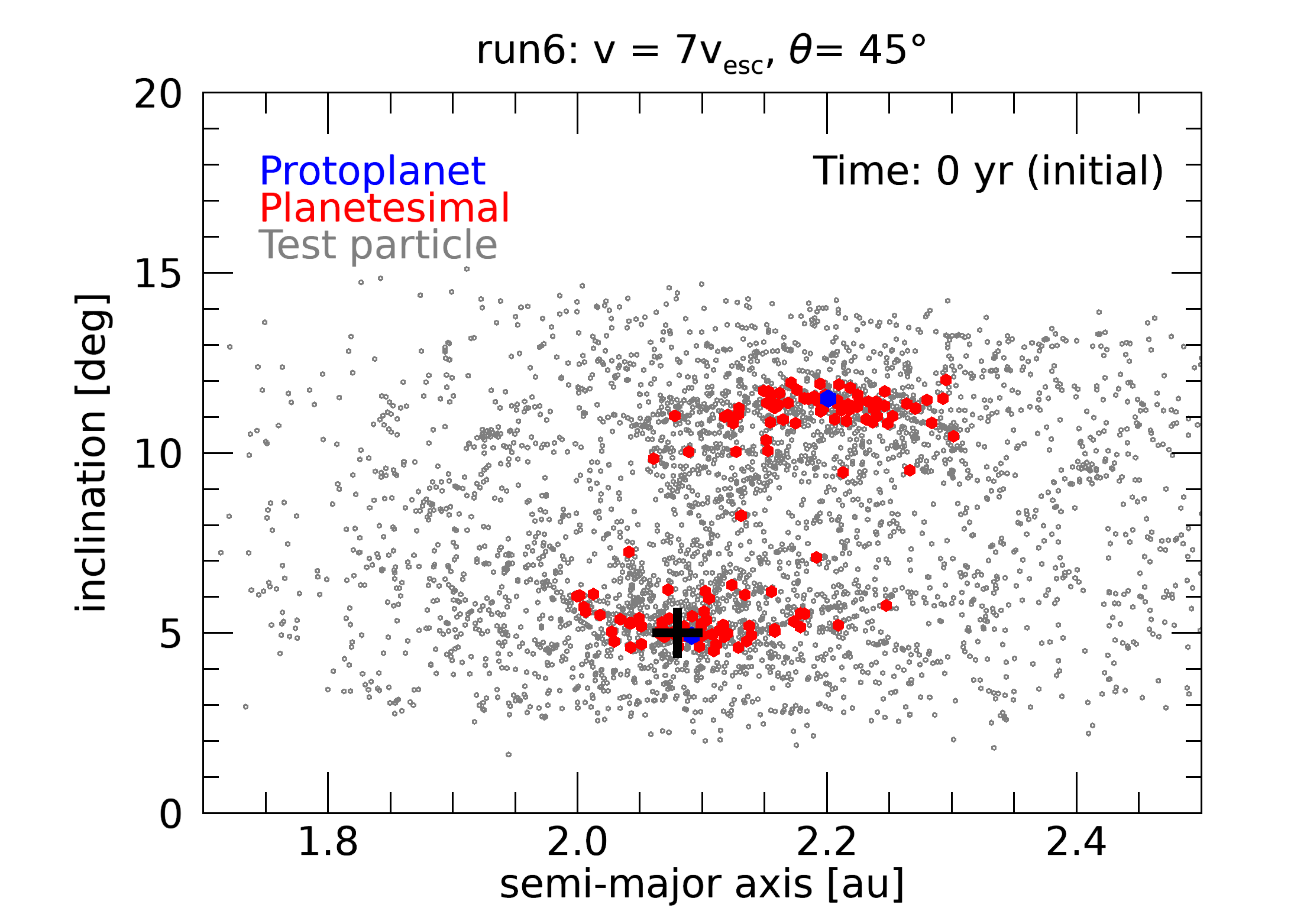
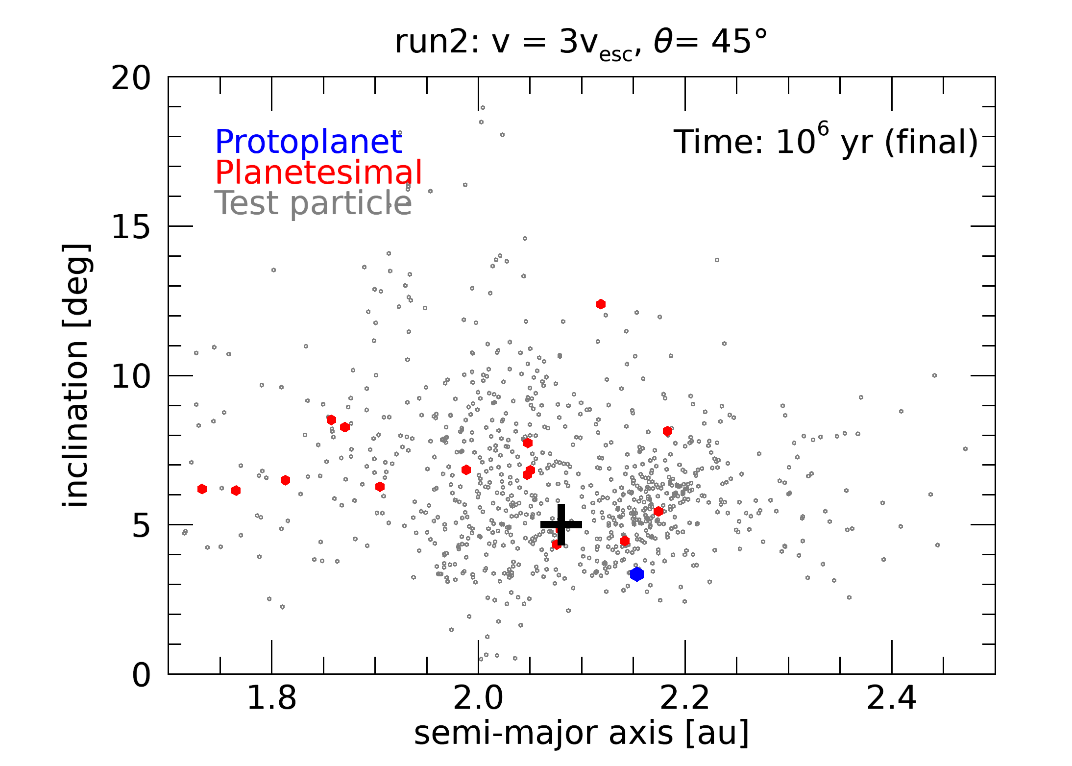
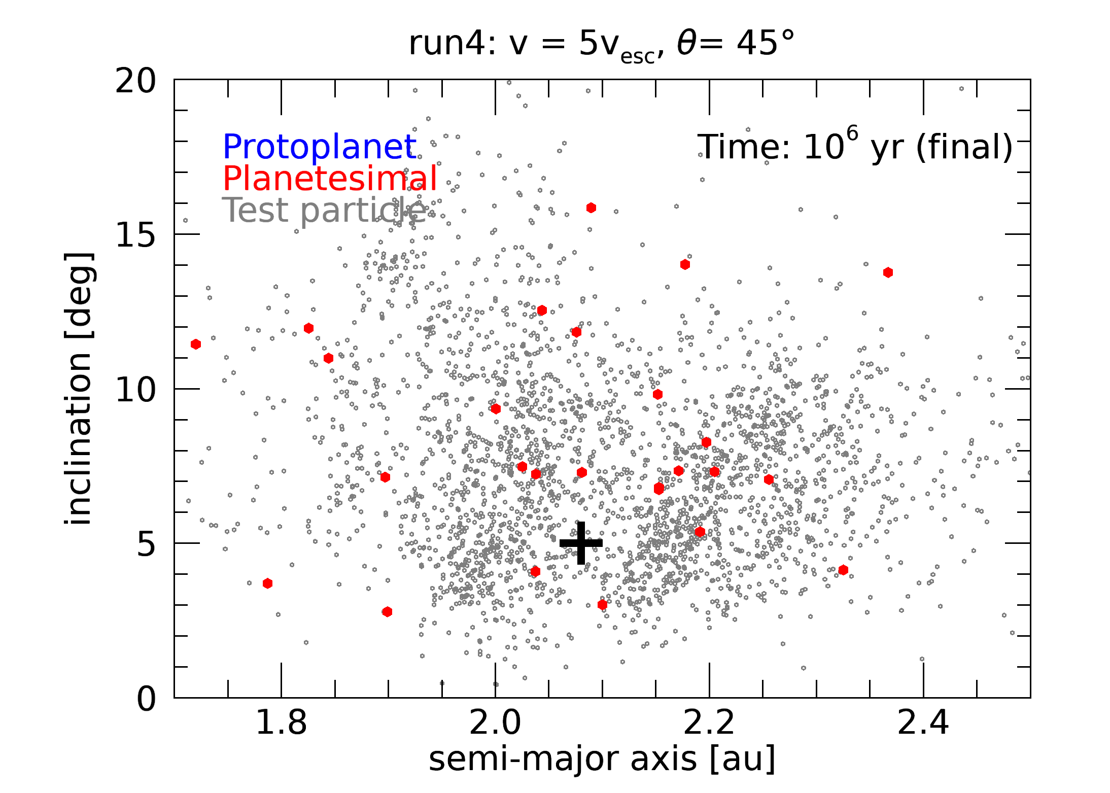
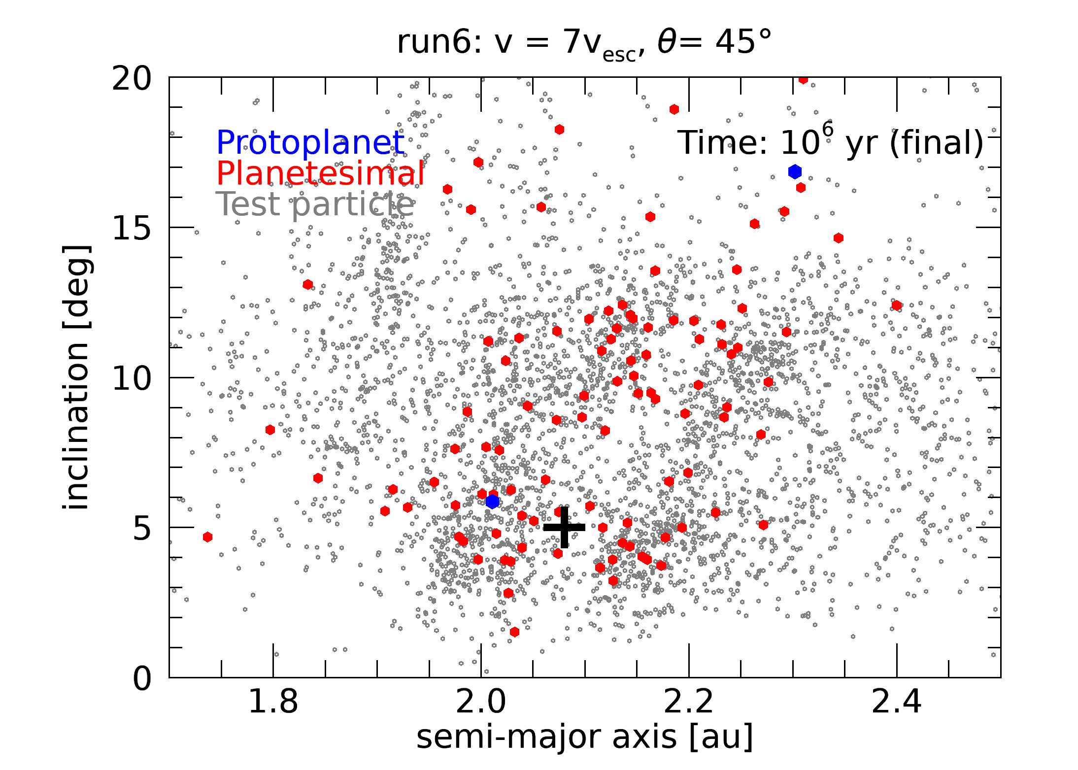
Figure 7: Same as in Fig. 6, but in the ($a-i$) plane.

In the $(a-e)$ planes, an interesting, checkmark-shaped structure forms in all cases for $t=0$. Both the massive and the massless bodies are confined to this shape. On the contrary, no well-defined shape appears on the ($a-i$) plane, where the fragments are scattered around the impact point. However, as velocity increases, distinct arcs become visible, particularly noticeable in the planetesimal distribution. The mechanism and theory behind the formation of the checkmark-shaped structure will be addressed in another article, it is out of the scope of the present paper. We also note that the semi-major axes of the smaller fragments span a wide range, e.g. for run1 it is approximately $a\in[1.75,2.5]$ au, which is a difference of $\Delta a\approx 0.75$ au, and about $1000$ times larger than in the $\mathrm{BC}xyz$ space. The higher the collision velocity, the wider the range over which the debris scatters. This fact plays a crucial role in the frequency of collisions with Earth, as discussed in Section 3 and demonstrated in Table 3. For all six runs the initial $e$ falls in the interval of $[0,0.25]$ while the $i$ is in the range of $[0,20]$ degree, c.f. Figs. 6 and 7. With an increase in $v$, the upper limits of the initial $e$ and $i$ grows.

The simulation parameters and initial orbital elements for the backward integrations are provided in Table 1. The planets were initially placed in their current orbits. Now we turn our focus to the determination of the fraction of collisions with an inflated Earth. The collision parameters $v,\,\theta$ were selected based on the results of Süli (2021), where the author performed 2D $N$-body simulations of planetary accretion. From the compiled statistics, the impact parameter $b=\sin\theta$ has a uniform distribution and the minimum of the impact speed is 1. Based on preliminary results from 3D planetary accretion simulations, the collision angle has a maximum of around 40 degrees, and the collision velocity reaches its maximum between 3 and 10. In light of these results, we selected the collision angles of 30 and 45 degrees, as well as the collision velocities of 3, 5, and 7, see Table 1 for details.

At the beginning, both the target and the projectile are initially in the $\nu_{6}$ resonance, raising the question of why they have not been ejected from there, given the relatively short timescale required for a significant increase in eccentricity (Morbidelli et al., 1994; Smallwood et al., 2018). On the other hand, Yoshikawa (1987) and Knezevic et al. (1991), have shown that the $\nu_{6}$ resonance is an efficient collector capable of capturing objects from the region between 2.4 and 2.7 au with moderate inclination ($15^{\circ}$ to $20^{\circ})$. Therefore, we may assume that the target and the projectile were formed further away, and when they reached the size of Ceres, they entered the $\nu_{6}$ resonance and eventually collided.

3 Results

We numerically integrate the trajectory and simulate the outcomes of fragments. Each simulation incorporates the presence of the three terrestrial planets Venus, Earth and Mars and two giants Jupiter and Saturn. The initial distribution of the eccentricities and inclinations are shown in the first and third rows of Figs. 6 and 7, respectively. The large black plus marks the impact location, blue circles indicate protoplanets, red ones represent planetesimals, and grey dots correspond to test particles. In the ($a-e$) plane, a distinct checkmark shape is clearly visible in the initial distribution of the generated debris. Additionally, it can be observed that collisions at higher velocities scatter the debris over a wider range along the $e$ axis, widening the arms of the checkmark. Increasing the collision angle from 30 to 45 degrees roughly halves the number of fragments. It’s also worth noting that the distribution of planetesimals concentrates on the right arm of the checkmark, and as the velocity ($v$) increases, it clusters towards the lower and upper boundaries of the checkmark shape. In general, after each collision, two protoplanets remain, with the exception of run5, where collision parameters are such that both the target and the projectile completely disintegrate into smaller fragments, leaving no protoplanets.

Fig. 7 similarly illustrates the initial and final states of collision remnants but in the ($a-i$) plane. With increasing velocity, arcs become apparent in the distribution of planetesimals.

At the end of the simulation ($t=10^{6}$ years), we also depicted the distribution of debris in both the ($a-e$) plane, (Fig. 6) and the ($a-i$) plane (Fig. 7). For better comparison, the displayed range is the same as the one used in the initial state. Consequently, some of the debris is not visible in the figures, even if it did not collide. The most prominent feature in the final state depicted in the figures is the depletion of the region around the $\nu_{6}$ secular resonance, between $\approx 2.05$ and $\approx 2.15$ au. This phenomenon is most pronounced in the ($a-e$) plane, as it is more sensitive to secular perturbations (see, for example, Figure 11 in Forgács-Dajka et al. (2022)) than in the ($a-i$) plane. Generally, dynamical maps are usually constructed using the maximum eccentricity method. In the ($a-i$) plane, the $\nu_{6}$ secular frequency is also beginning to manifest itself and is expected to become more pronounced with longer integration times.

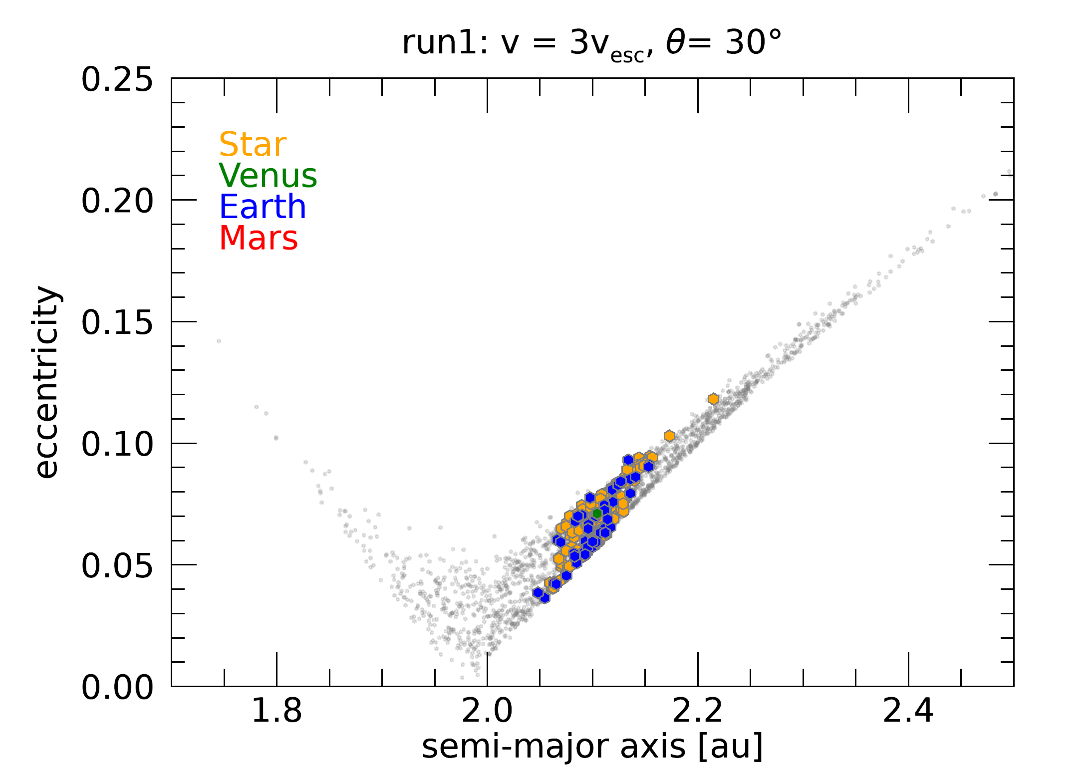
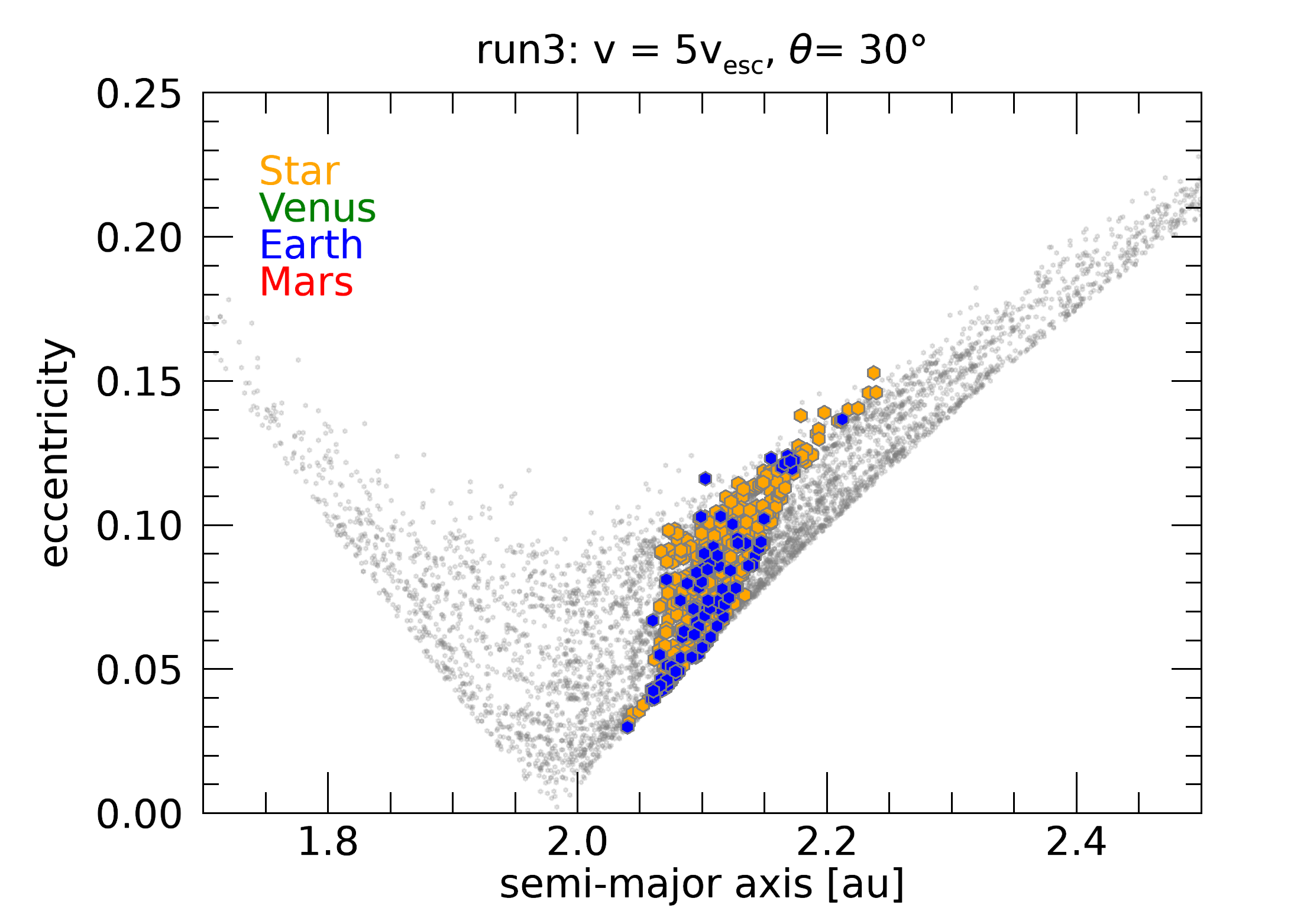
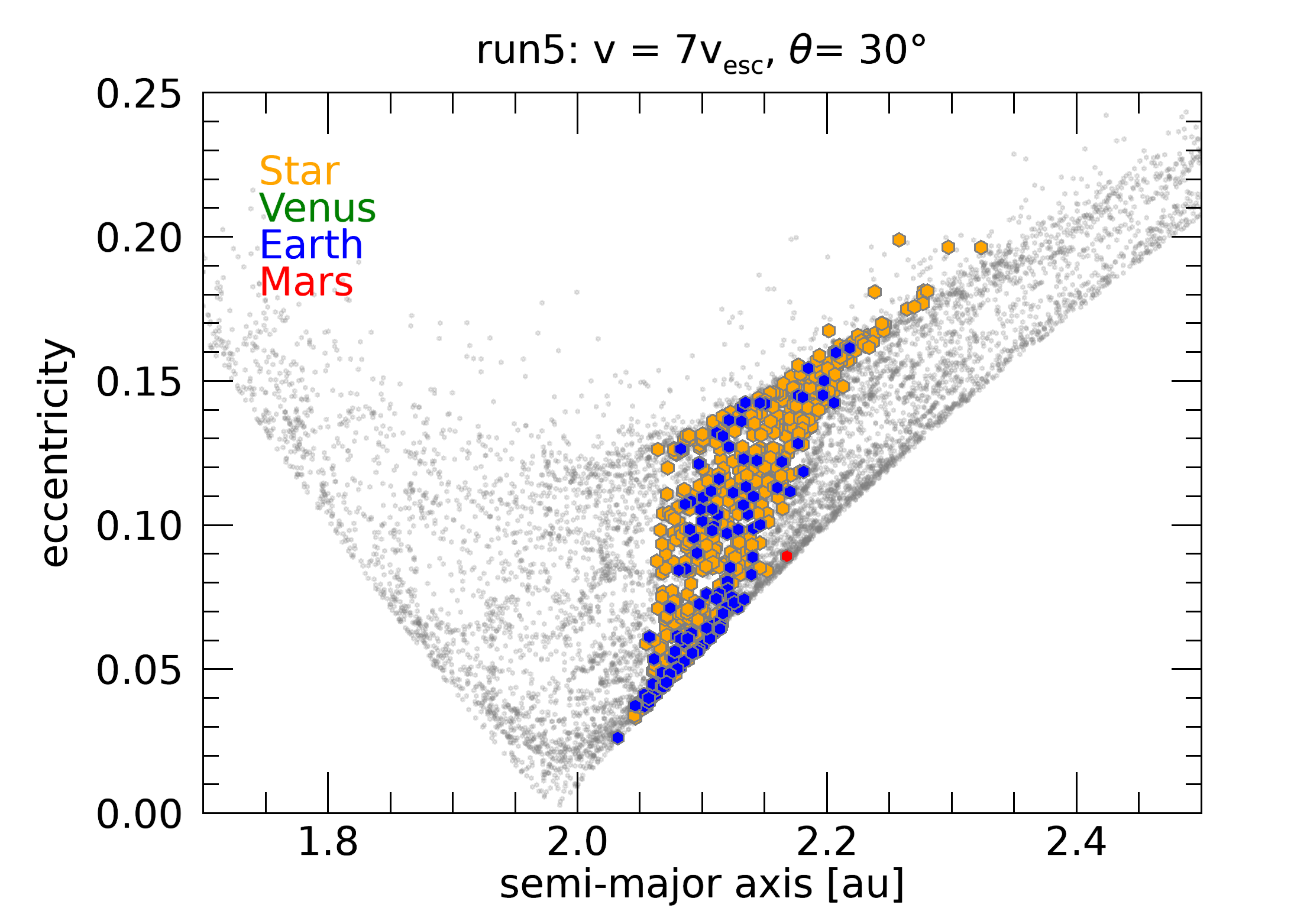
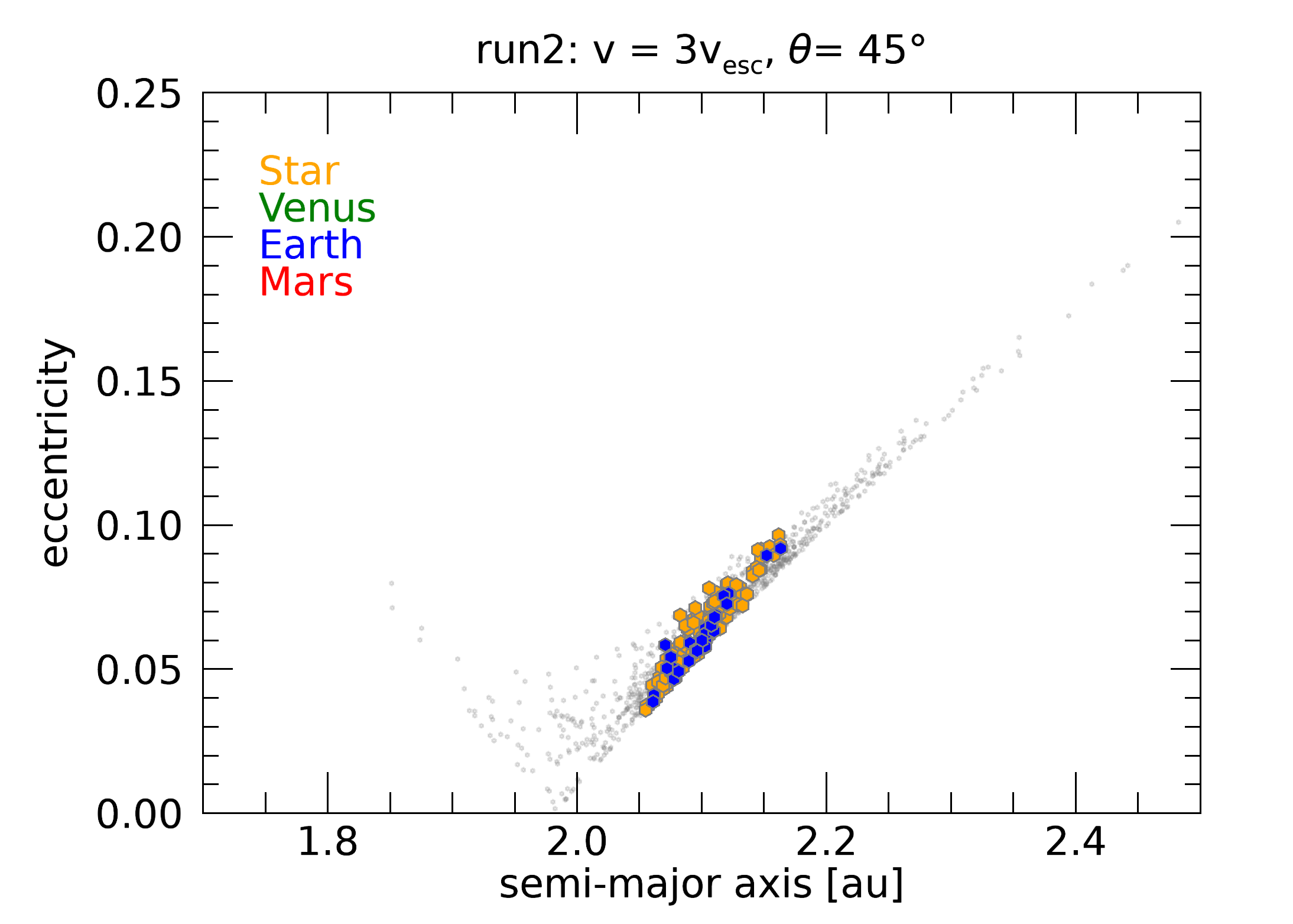
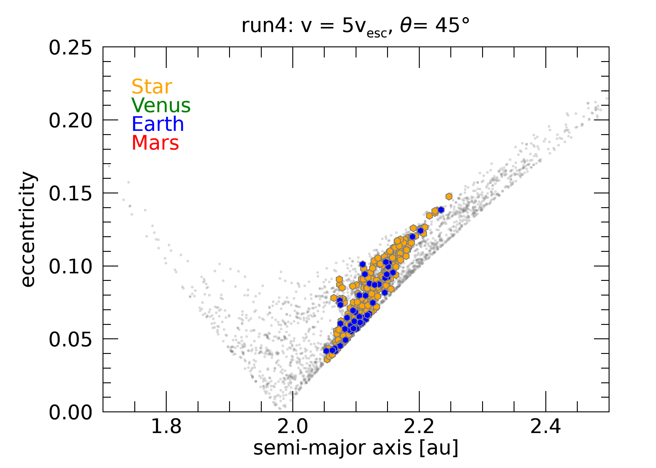
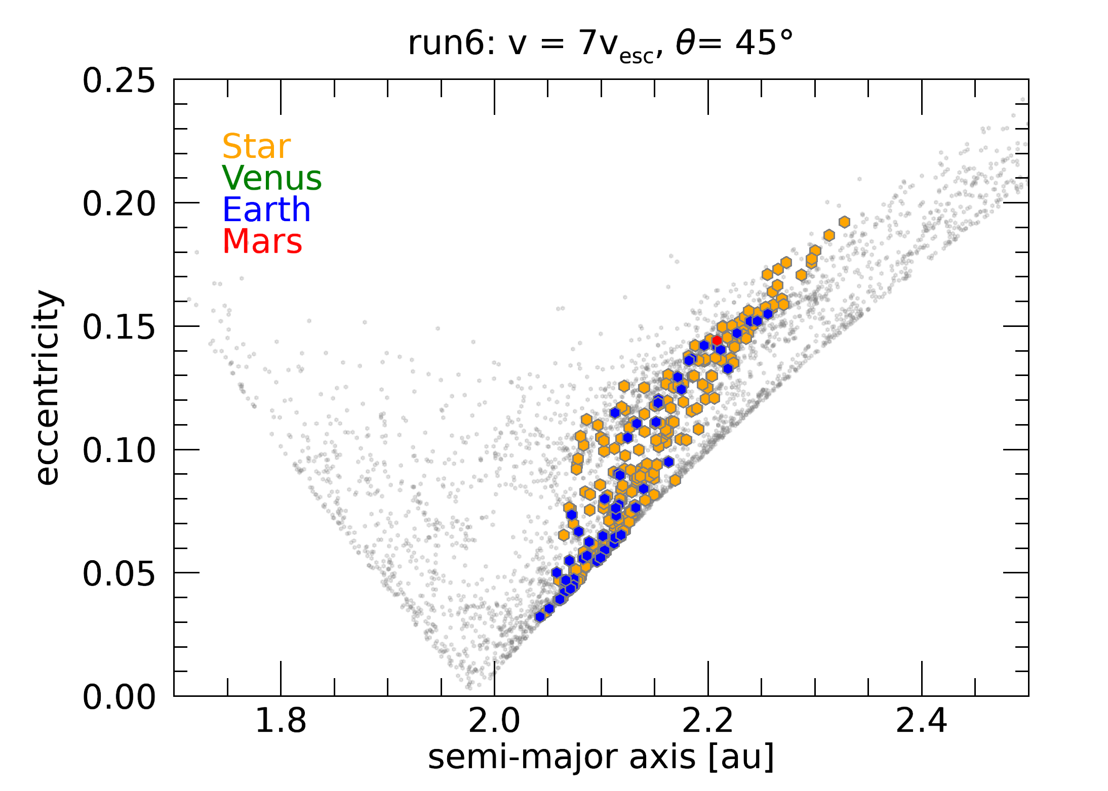
Figure 8: The positions of the fragments in the ($a-e$) plane that collided with the Sun or one of the rocky planets for different impact velocities and angles (see Table 2). The upper panels depict simulations with $\theta=30^{\circ}$ while the lower panels for $\theta=45^{\circ}$. The colors indicate the fragments colliding with the different celestial bodies, while the initial position of all bodies involved in the $N$-body simulation is indicated in grey in the background.

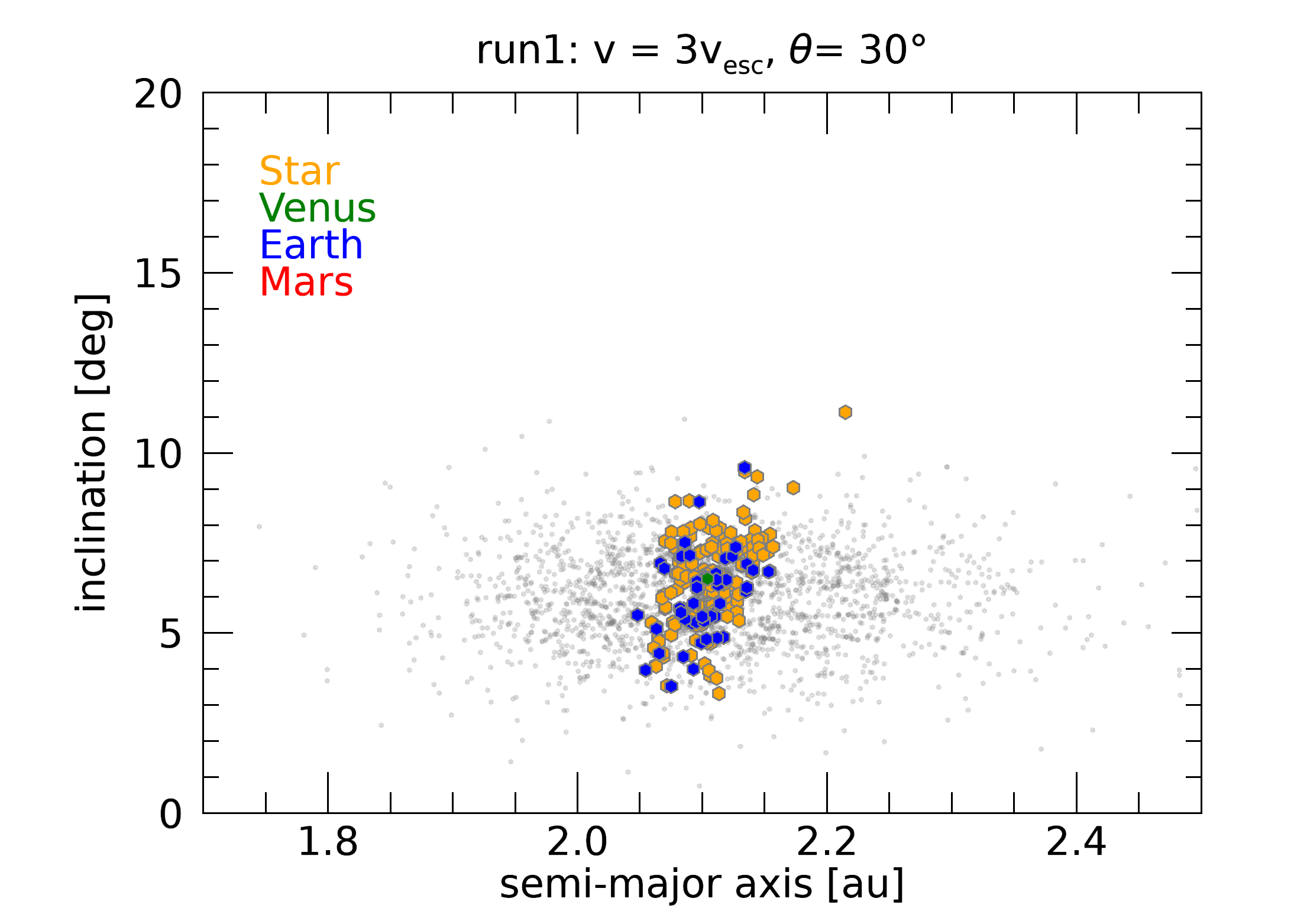
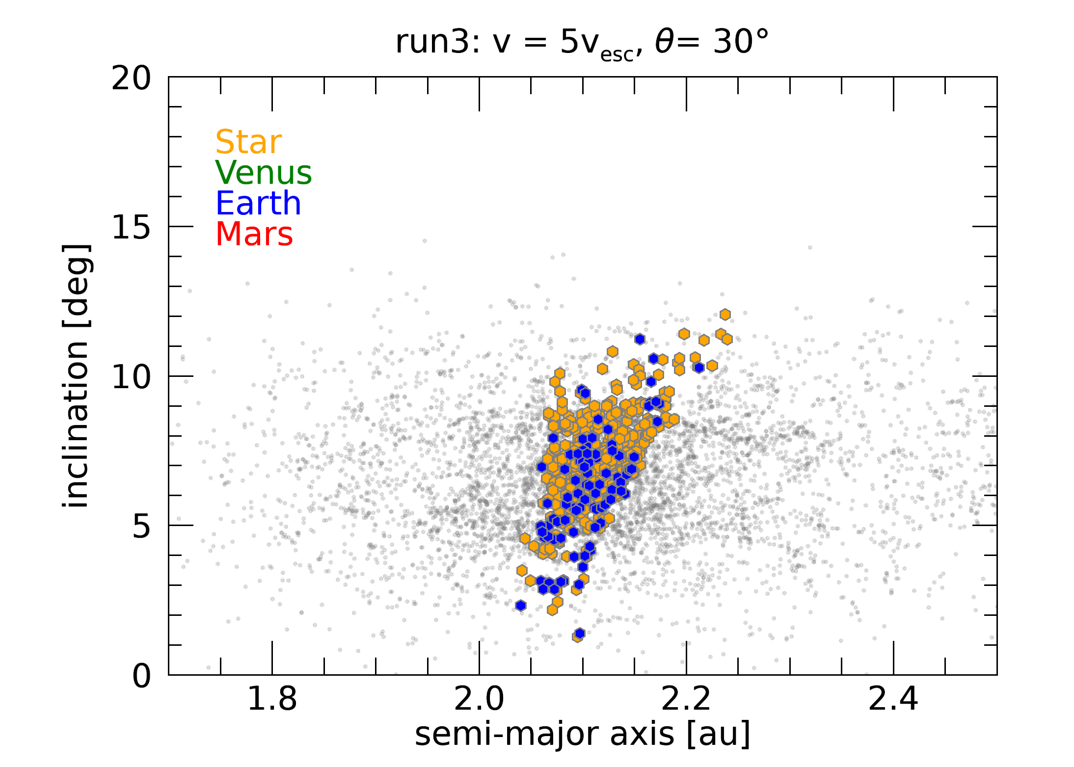
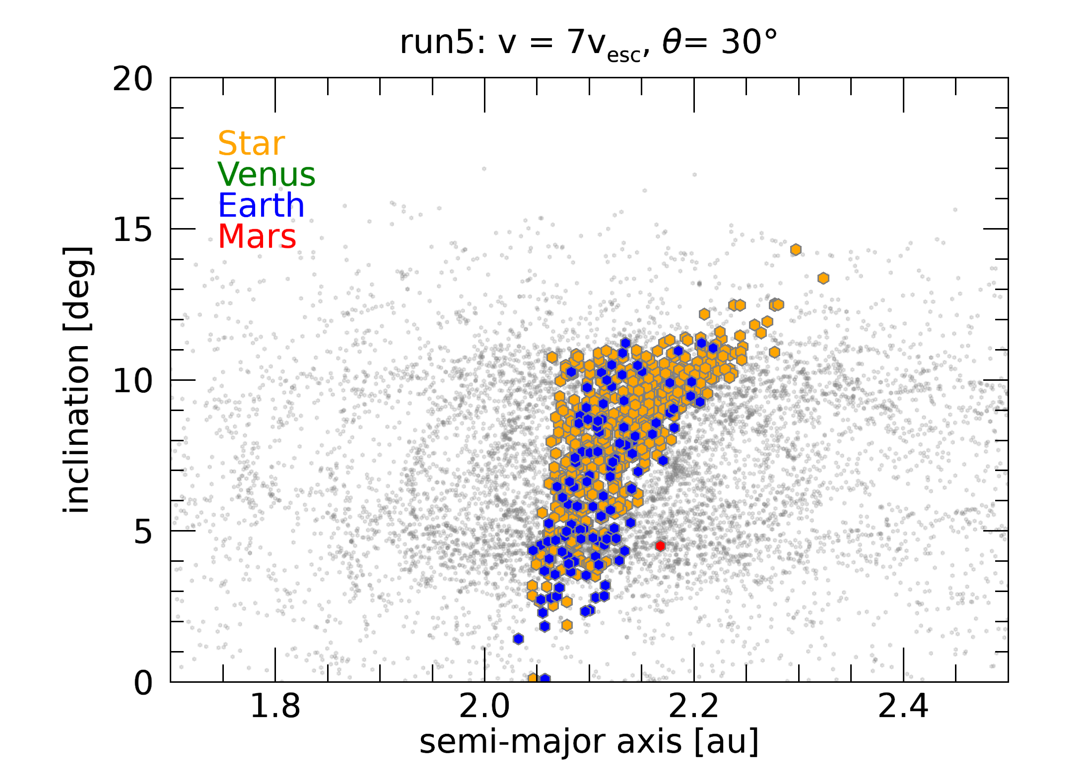
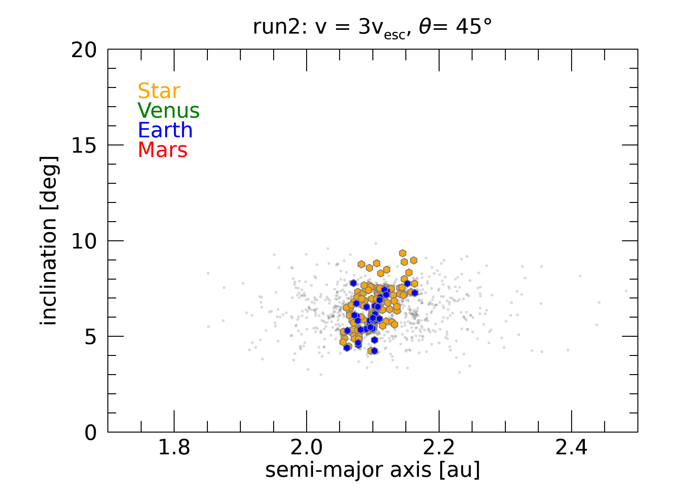
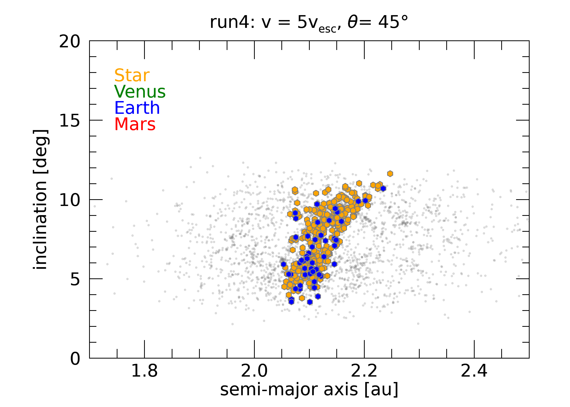
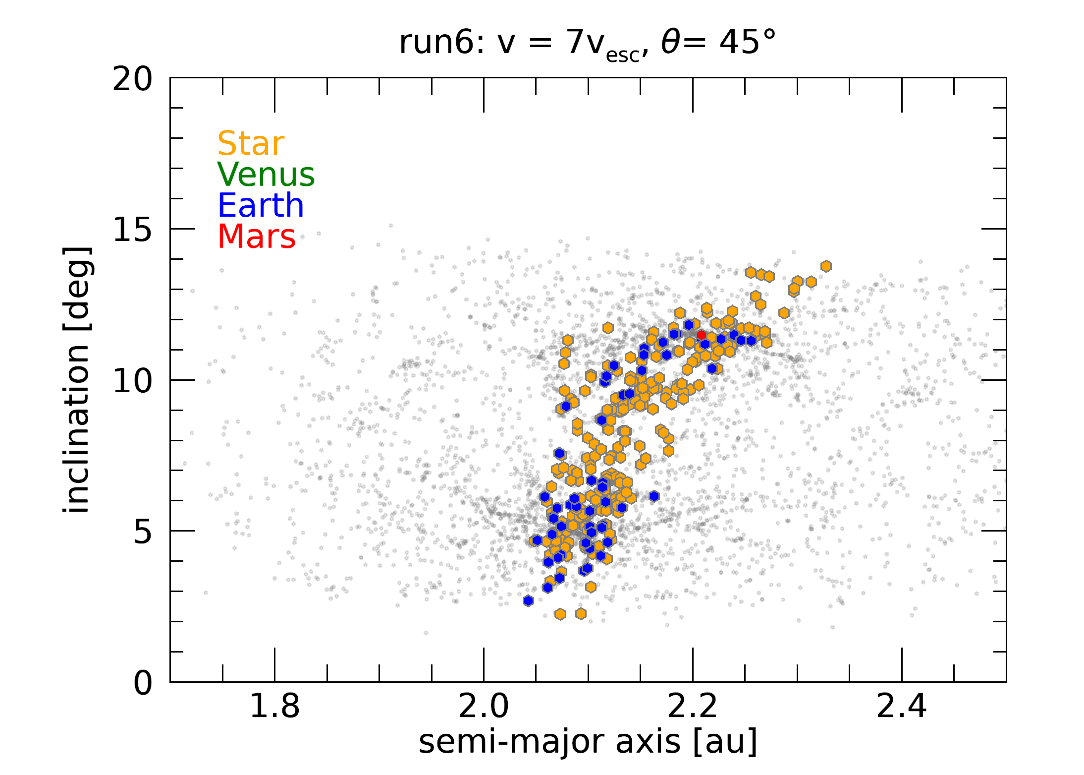
Figure 9: Same as in Fig. 8, but in the ($a-i$) plane.

In Figs. 8 and 9 you can see the initial positions of celestial bodies that collided with the Sun or one of the rocky planets. These figures clearly illustrate the extent and shape of the $\nu_{6}$ secular resonance. The $\nu_{6}$ resonance becomes more prominent as the initial fragment distribution covers a larger area in the ($a-e$) plane. This inspires us to conduct further research in which the entire area will be mapped with test particles to precisely determine the shape and extent of the $\nu_{6}$ resonance in both the ($a-e$) and ($a-i$) planes. In Fig. 9 the colored region delineated by colliding bodies extends further to larger $a$-values as inclination increases. This observation aligns with Figure 1a in the study by Froeschle & Scholl (1986), although in our figure, the vertical axis represents the osculating inclination while in Froeschle & Scholl (1986)’s figure, it represents the proper inclination.

According to the results presented in ML, there were no collisions observed when considering the actual radius of the Earth ($R_{\oplus}=6371$ km). Therefore, based on their results, we used a 10 times larger radius for the Earth $R_{\mathrm{Earth}}=10R_{\oplus}$ in the simulations to ensure that collisions occur. The radii of the other planets were taken as their actual values. We considered a particle to hit the Sun if its astrocentric distance became smaller than 0.3 au.

We will use the estimation employed by ML to determine the number of objects colliding with a real-sized Earth based on the number of objects colliding with an inflated Earth of size $10R_{\oplus}$. The estimation resulted in a factor $f\approx 20$ for the position of the $\nu_{6}$ secular resonance.

According to Table 2 it can be observed that at $\theta=30^{\circ}$, approximately twice as many fragments are produced compared to the case of $\theta=45^{\circ}$ collision for all three impact velocities. A significant portion of the debris collides with larger fragments, primarily with the remnants of the collided bodies, which are the two largest objects in the debris cloud. The sum of these collisions can be found in the table under the $N_{\mathrm{TP}}$ header (the subscript TP stands for target and projectile). This process, known as reaccretion, returns a substantial fraction of the mass back to the target and projectile, the specific mass can be found in Table 5. The reaccretion occurs within a few years following the collision, and after that, debris rarely impacts on the remnants of the impacted bodies. However, in the following years collisions still occur between smaller fragments and test particles, but the rate of these collisions decline with time.

Overall, based on the table, it can be concluded that a smaller impact angle, representing a more frontal collision, generates more debris than a larger impact angle, which corresponds to a more tangential collision. Of course, for both impact angles, higher velocities further increase the amount of debris, and they scatter more widely in both the ($a-e$) and ($a-i$) planes. The wider the range in which the fragments are scattered along the semi-major axis, the proportionally fewer of them end up in the $\nu_{6}$ resonance. Therefore, in the case of higher-velocity collisions, fewer fragments enter the $\nu_{6}$ resonance region.

The outcomes for $v=3$, $\theta=30^{\circ}$ and $\theta=45^{\circ}$ are shown in the left panels of Fig. 11 and the data are listed in the first two rows of Table 2. It is clear that the majority of collisions occur with the Sun and with Earth. The number of collisions with the Sun significantly exceeds the number of impacts with Earth. Within the simulation time span of 1 Myr, there were a total of 47 impacts on the Earth, for $\theta=30^{\circ}$, while 33 impacts on Earth for $\theta=45^{\circ}$. In the case of $v=5$ there were 95 and 52 Earth impacts for $30^{\circ}$ and $45^{\circ}$ impact angles, respectively. For the case of $v=7$, the measured values are 116 and 58, respectively. For the Sun, these numbers are as follows: in the case of run1 and 2, 178 and 181; in the case of run3 and 4, 427 and 307; while in the last two runs, 600 and 245. The observed trend is that with more oblique impacts, a larger number of fragments are produced and as a result of this the number of impacts also increases. The number of impacts into the giant planets are in close agreement with the results of ML and are in the order of unity.

We have calculated two ratios using two different benchmarks to measure the chance of collision with Earth. In the first case $P_{10}=N_{\mathrm{E}}/(N_{\mathrm{pp}}+N_{\mathrm{pl}}+N_{\mathrm{tp}})$, while in the second one $P_{10}^{\star}=N_{\mathrm{E}}/N_{\mathrm{event}}$ In order to directly compare the results with those of ML, the latter definition matches what was used in the ML paper. Both $P_{10}$ and $P_{10}^{\star}$ characterize the likelihood of objects impacting the inflated Earth, thus these ratios can be considered as a loosely defined probability of impact with Earth. The calculated values of $P_{10}$ and $P_{10}^{\star}$ are listed in Table 3. The measured $P_{10}$ decreases with increasing $v$, the maximum is $\approx 0.0258$ ($v=3,\,\theta=45^{\circ}$), the minimum value is $\approx 0.0111$ ($v=7,\,\theta=30^{\circ}$), thus both the minimum and the maximum fall into the same order of magnitude. The decreasing trend is a consequence of the fact that at higher velocities, the fragments making up the debris scatter over a larger range along the semi-major axis (as mentioned above). Consequently, proportionally fewer fragments enter the $\nu_{6}$ resonance, resulting in fewer fragments on Earth-crossing orbits.

The ratio $P_{10}^{\star}$ does not follow a similar trend, it fluctuates around a mean value of 0.0876 with a standard deviation of 0.0112. To adjust for the inflated Earth, these values need to be divided by a factor of $f=20$, as described above. The computed ratios $P$ and $P^{\star}$ are given in the last two columns of Table 3. Since $P$ and $P^{\star}$ differs by a factor of $f$ they follow the same pattern as $P_{10}$ and $P_{10}^{\star}$.

In general, the histograms in Fig. 11 are similar. In the time following the first collision, approximately equal amounts of debris collide with both the Earth and the Sun. However, over a period of a few hundred thousand years, this ratio significantly shifts in favour of collisions with the Sun. The earliest event occurs between $10^{5}$ and $2\cdot 10^{5}$ years, indicating that it takes roughly this amount of time for the first debris fragments from the $\nu_{6}$ resonance to reach the inner Solar System. Interestingly, in the run1 simulation, the first collision occurs with Venus at $t\approx 1.107\cdot 10^{5}$ years, followed by a longer period without any event until around $t\approx 4\cdot 10^{5}$ years. From this point on, debris fragments collide with both the Earth and the Sun.

We note that a few impacts on the other rocky planets were also detected, 1 impact into Venus (green bar) for run1 and 2 collisions with Mars both in run5 and run6 (red bar). Mars collision occurs only for the $v=7$ cases.

Figure 10: An example of a collision tree, showing the mass of the fragments (gray-black) and of the remnants of the target (solid blue line) vs. time in run5. After a collision is simulated with SPH, the orbital evolution of the fragments is tracked using our $N$-body integrator and if a collision is detected then the two bodies merge. This figure shows only a part of the whole collision tree, where the mass evolution of some fragments that eventually impact the target are depicted by gray-black lines. Every jump in the lines correspond to a collision.

In Fig. 10 a part of the collision history of an individual protoplanet is visualised using a collision tree. The collision events are plotted only for $t\leq 30$ years. The gray-black lines show the mass of fragments as a function of time, while the blue line shows the increase in mass of the target body left after the SPH simulation. In the figure, for clarity, only one collision tree has been drawn. The smaller fragments merge together during the first 10 years, forming a larger body with mass $\approx 3\cdot 10^{19}$ kg, which hits the target at $t\approx 23$ years. Notice that initially several fragments have the same mass, thus gray-black lines are overlap in the beginning of the simulation.

Table 2: The simulation outcomes with $R_{\mathrm{Earth}}=10R_{\oplus}$ for $T=10^{6}$ years. The first column contains the names of the simulations. Columns 2 and 3 show the impact velocity $v$ and angle $\theta$, respectively. Column 4 represents the total number of bodies (including the Sun and 5 planets) $N$. Columns 5,6 and 7 display the number of protoplanets $N_{\mathrm{pp}}$, planetesimals $N_{\mathrm{pl}}$ and test particles $N_{\mathrm{tp}}$ respectively. Column 8 - 13 contains the number of events (outcomes) $N_{\mathrm{event}}$, fragments that collided with the Sun $N_{\mathrm{Sun}}$, Venus $N_{\mathrm{V}}$, Earth $N_{\mathrm{E}}$, Mars $N_{\mathrm{M}}$ and Jupiter or Saturn $N_{\mathrm{JS}}$, respectively. Column 13 lists the number of collisions $N_{\mathrm{TP}}$ with the remnants of the target and projectile.

Sim.	$v[v_{\mathrm{esc}}]$	$\theta$ [deg]	$N$	$N_{\mathrm{pp}}$	$N_{\mathrm{pl}}$	$N_{\mathrm{tp}}$	$N_{\mathrm{event}}$	$N_{\mathrm{Sun}}$	$N_{\mathrm{V}}$	$N_{\mathrm{E}}$	$N_{\mathrm{M}}$	$N_{\mathrm{JS}}$	$N_{\mathrm{TP}}$
run1	3.0	30	2662	2	102	2552	612	178	1	47	0	0	210
run2	3.0	45	1283	2	34	1241	383	181	0	33	0	0	101
run3	5.0	30	6847	2	44	3125	1067	427	0	95	0	0	208
run4	5.0	45	3176	2	518	6321	526	307	0	52	0	1	156
run5	7.0	30	10502	0	927	9569	1576	600	0	116	2	2	134
run6	7.0	45	4442	2	155	4279	573	245	0	58	2	0	199

Table 3: The simulation results with $R_{\mathrm{Earth}}=10R_{\oplus}$ for $T=10^{6}$ years. The first column contains the names of the simulations. Columns 2 and 3 show the collision probability with an inflated Earth $P_{10}=N_{\mathrm{E}}/(N_{\mathrm{pp}}+N_{\mathrm{pl}}+N_{\mathrm{tp}})$ and $P_{10}^{\star}=N_{\mathrm{E}}/N_{\mathrm{event}}$. Columns 4 and 5 list the approximate rate with actual size Earth $P=P_{10}/f$ and $P^{\star}=P_{10}^{\star}/f$, where $f=20$.

Sim.	$P_{10}$	$P_{10}^{\star}$	$P$	$P^{\star}$
run1	0.0177	0.0768	0.00088	0.00384
run2	0.0258	0.0862	0.00129	0.00431
run3	0.0139	0.0890	0.00069	0.00445
run4	0.0164	0.0989	0.00082	0.00494
run5	0.0111	0.0736	0.00055	0.00368
run6	0.0131	0.1012	0.00065	0.00506

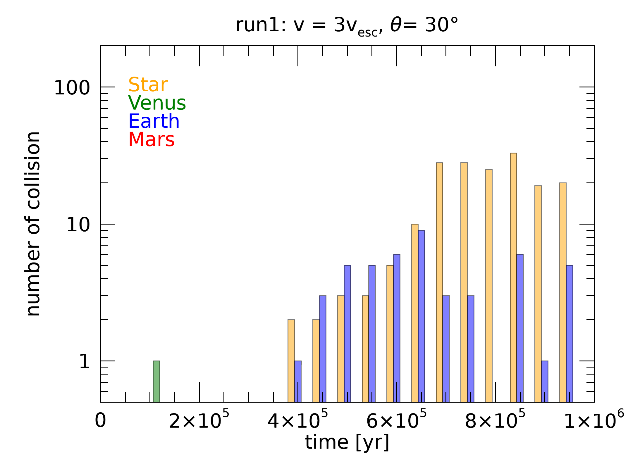
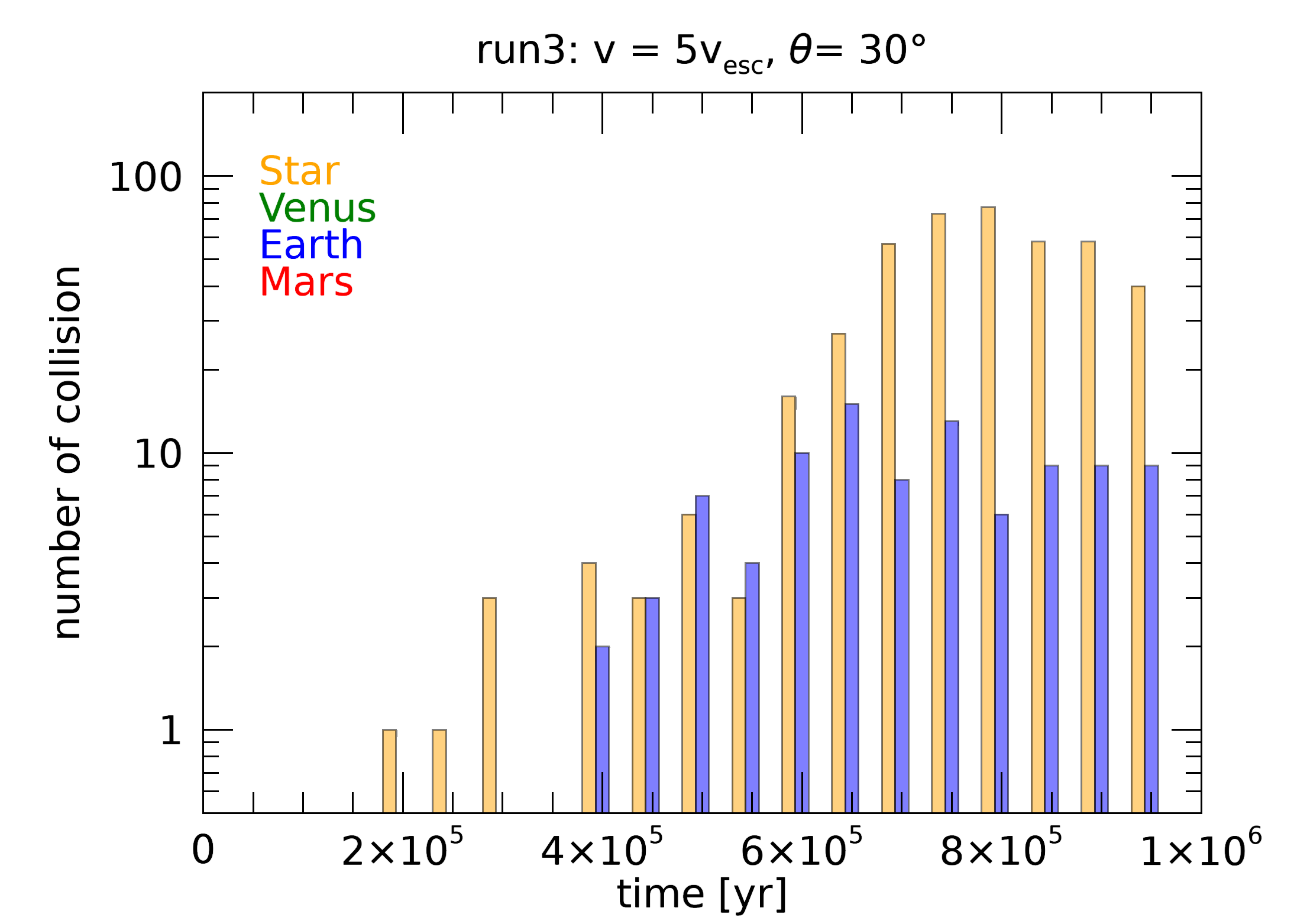
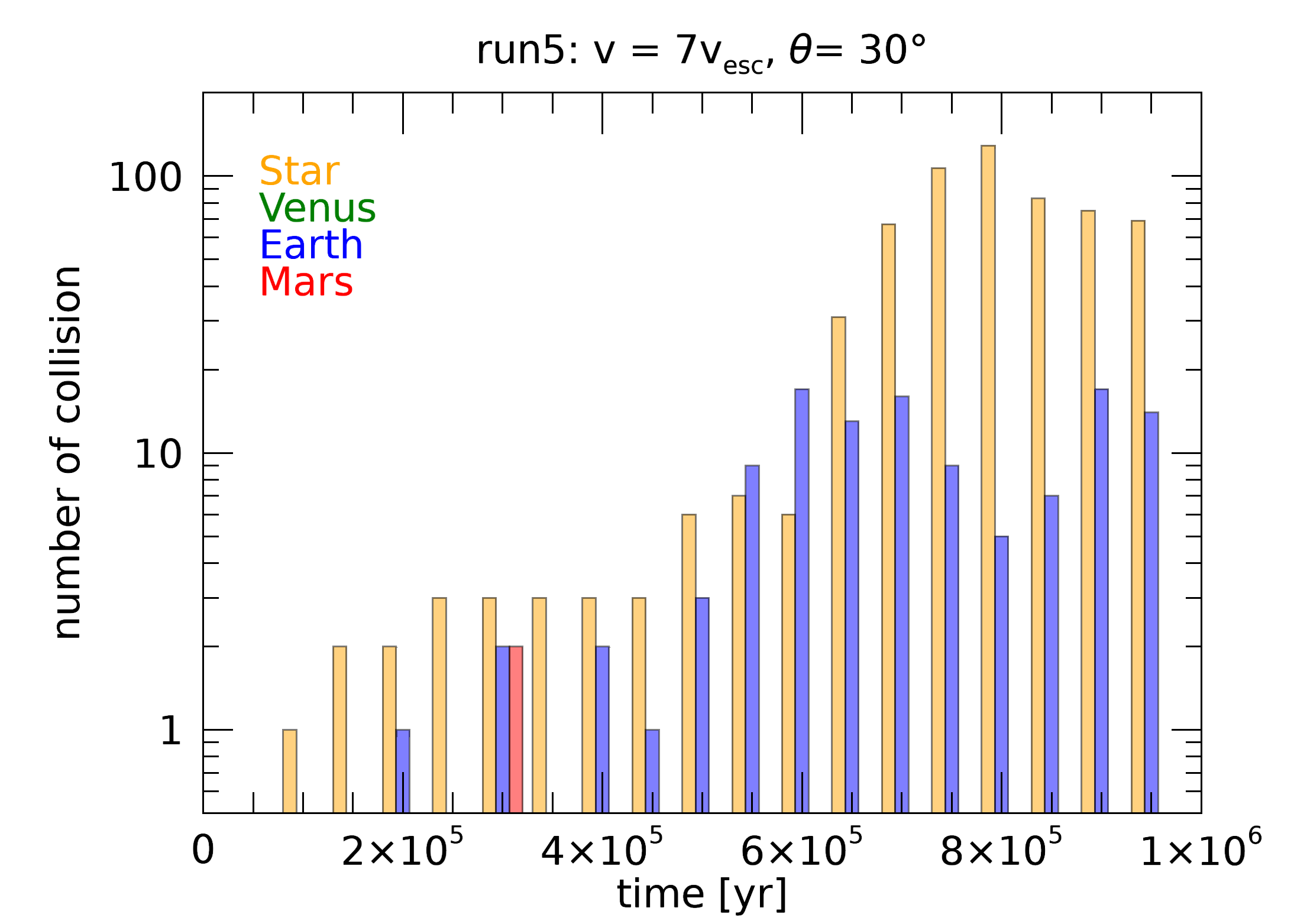
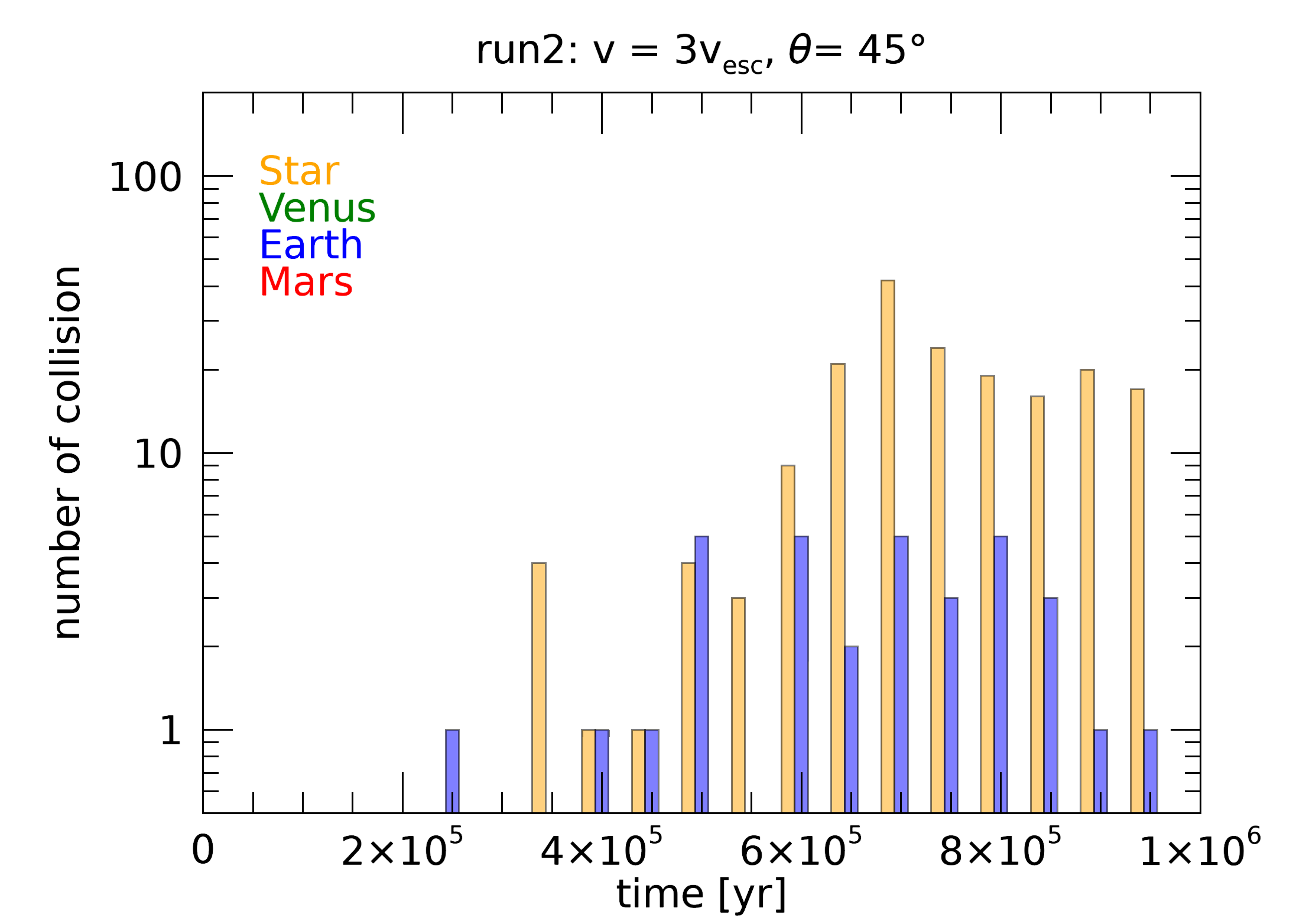
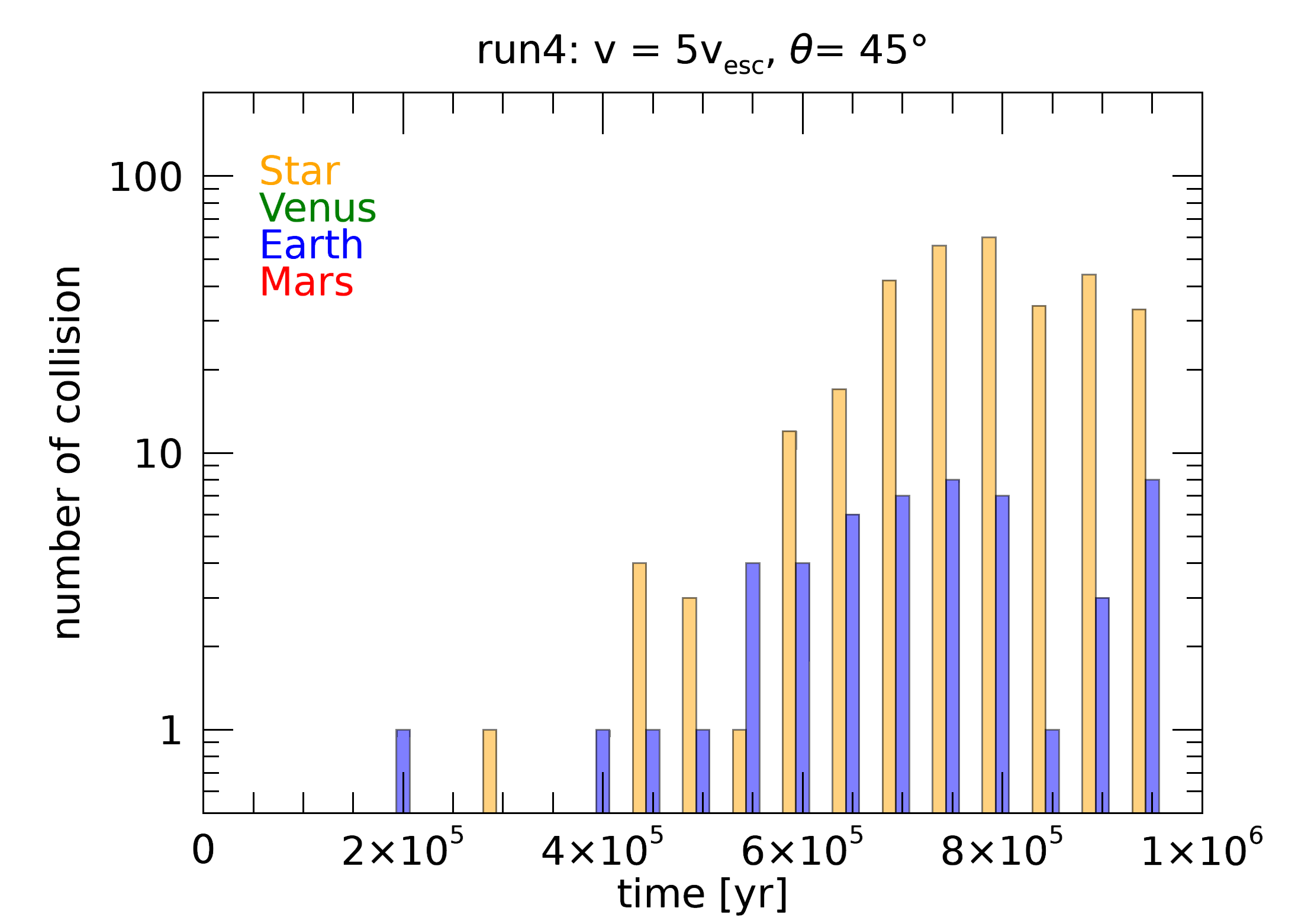
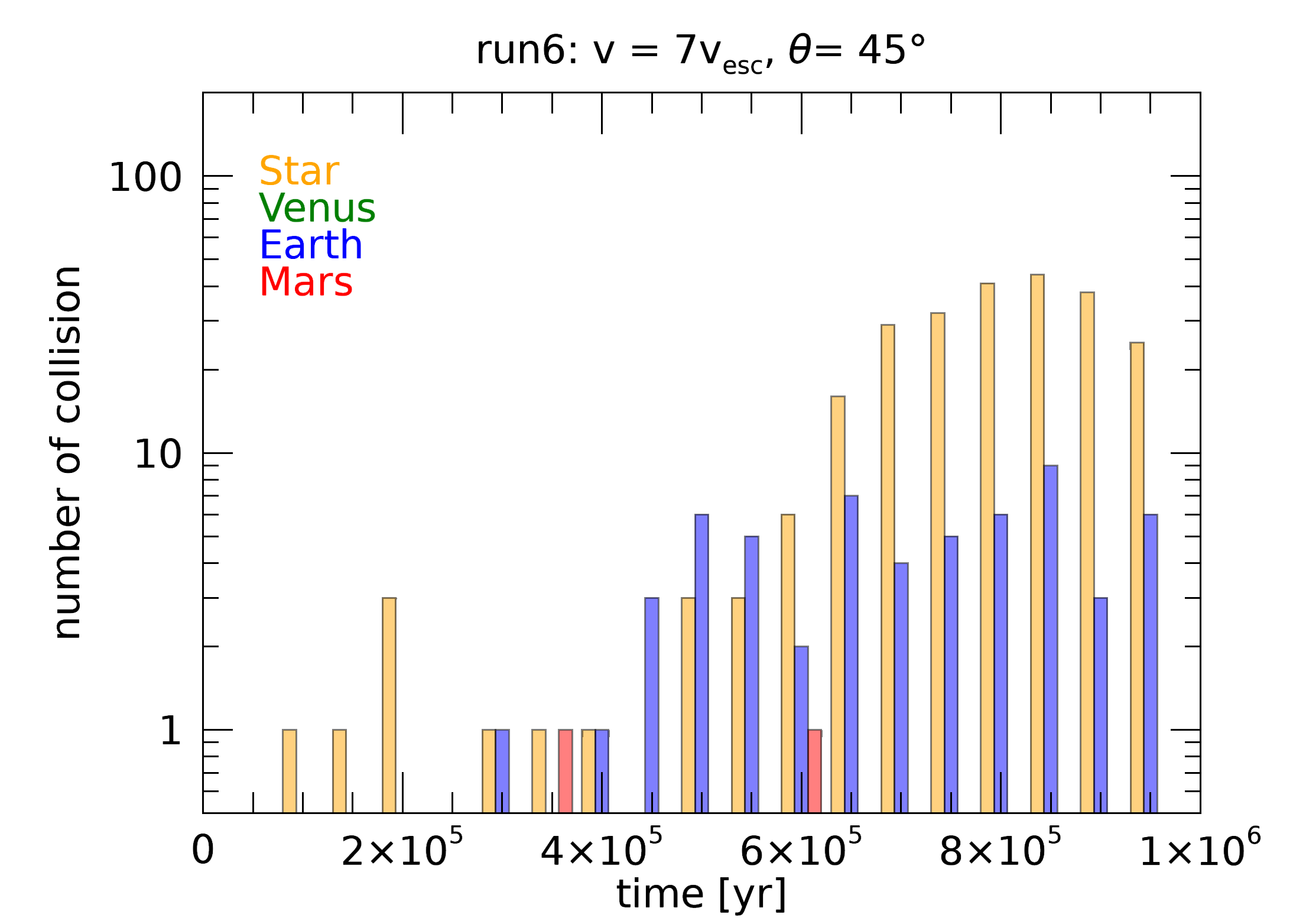
Figure 11: The event history of the $N$-body simulations are binned into 50 kyr time intervals for the different impact speed and angle, see Table 2. The upper panels depict simulations with $\theta=30^{\circ}$ while the lower panels for $\theta=45^{\circ}$. The Earth radius is $10R_{\oplus}$ for all cases, the other planets have their actual radius. In the plots, the yellow bars show the number of fragments that hit the Sun, while the green, blue and red bars represent asteroids colliding with Venus, Earth and Mars, respectively.

3.1 Water delivery by fragments

As previously stated, the inner region of the original planetesimal disk is dry, therefore several explanations for the presence of water on Earth were devised. According to a group of models explaining the origin of Earth’s water, the source is located in the outer regions of the Solar System. Among these models, the external pollution model is currently widely accepted, which successfully accounts for the quantity and chemical composition of water on Earth and is consistent with various theories of Solar System formation. The present study seamlessly fits into this and the other models too, assuming that Earth’s water originate from the outer Solar System, as collisions between protoplanets are inevitable and frequent during the early stages of planetary evolution.

The composition of the bodies in the asteroid belt depends on the radial distance, as indicated by studies e.g. Kerridge (1985); Gradie & Tedesco (1982); DeMeo & Carry (2014). The snowline $r_{\mathrm{SL}}$, which is approximately 2.7 au from the Sun is a boundary beyond which volatile substances, such as water can condense and freeze. The inner regions, $r<r_{\mathrm{SL}}$ au are predominantly populated by S-type asteroids, their fraction of water is typically quite low, with estimates ranging from less than 0.1% to 1% by mass. In contrast, beyond $r_{\mathrm{SL}}$ the asteroid belt are dominated by C-type asteroids, which generally have a water fraction $f_{\mathrm{water,C}}$ of approximately 10% by mass (Kerridge, 1985). The current mass of water in Earth’s oceans is $2.5\cdot 10^{-4}\mathrm{M_{\oplus}}$, while the mass of the asteroid belt is only $4.5\cdot 10^{-4}\mathrm{M_{\oplus}}$ despite covering a vast region from 2 to 4 au (Krasinsky et al., 2002; Kuchynka & Folkner, 2013). This mass is orders of magnitude smaller than what would be predicted by models of planet-forming disks, such as the minimum-mass solar nebula model (MMSN) (Weidenschilling, 1977; Hayashi, 1981). We note that actually the MMSN is not a nebula, but represents a protoplanetary disc with solar composition containing the requisite amount of metals for the formation of the eight planets within the solar system, including the asteroid belts. In order to determine the original total mass of solids in the asteroid belt the MMSN were used in which the surface density of solids is

$$\Sigma_{\mathrm{solid}}=f_{\mathrm{n}}f_{\mathrm{ice}}\Sigma_{1}r^{-\frac{3}{2}},$$ (16)

where $f_{\mathrm{n}}$ is a nebular mass scaling factor, $f_{\mathrm{ice}}$ is the ice condensation factor, $\Sigma_{1}$ is the surface density of solids at 1 au and $r$ is the distance from the Sun. According to Hayashi (1981) $\Sigma_{1}=7.1\,\mathrm{gcm^{-2}}$, $f_{\mathrm{ice}}=1$ for $r\leq r_{\mathrm{SL}}$ and $f_{\mathrm{ice}}=4.22$ for $r>r_{\mathrm{SL}}$. By integrating Eq. (16) from 1.55 (3 times the Mars’ Hill radius) to 4.1 au (3 Hill radii from Jupiter) we obtain the mass of solid material

$$M_{\mathrm{solid}}=f_{\mathrm{n}}\Sigma_{1}\int_{0}^{2\pi}d\theta\int_{1.55}^{4.1}f_{\mathrm{ice}}r^{-\frac{3}{2}}\,dr=6.69f_{\mathrm{n}},$$ (17)

in $\mathrm{M_{\oplus}}$ units. Despite its widespread use, the MMSN model has several limitations. It assumes planets gathered all nearby solids, but only some of the solid material were in planetesimals, while others were in the form of dust which was later lost as the solar nebula’s dissipated. Adjusting for this lost mass relies on the fraction of solids in planetesimals. However, the model assumes that all planetesimals were accreted, which may not hold true for terrestrial planets. In the region between 0.4 and 4 au, where terrestrial planets were forged, simulations show significant, $\geq 50\%$ mass loss and redistribution during the final assembly stage (Raymond et al., 2005). The asteroid belt and the region near Mercury have also been depleted of solids at some point (Weidenschilling, 1977). This suggests that the MMSN model doesn’t fully capture the complexities of planet formation in these areas.

Thus, for the MMSN $f_{\mathrm{n}}=1$, so Eq. (17) results in 6.69 $\mathrm{M_{\oplus}}$ which is the minimum mass required to forge the terrestrial planets. In light of the above, it is evident that $f_{\mathrm{n}}>1$, and simulations examining the formation of the solar system suggest that $2\leq f_{\mathrm{n}}\leq 3$ (see e.g.  Fogg & Nelson, 2005, 2007; Raymond et al., 2005; Raymond & Izidoro, 2017). Since S-type asteroids are very dry, we are interested only in C-type asteroids which are primarily located beyond the snowline. The mass $M_{\mathrm{C}}$ contained in $r_{\mathrm{SL}}<r<4.1$ au is $M_{\mathrm{C}}=5.38f_{\mathrm{n}}\,\mathrm{M_{\oplus}}$ and it is composed predominantly of C-type asteroids.

If we focus only on C-type asteroids and assume that they entered the $\nu_{6}$ resonance via some mechanisms (e.g. chaotic diffusion, gravitational scattering, etc.), the estimation for the maximum amount of water that could be delivered to Earth can be given by the following formula (see Eq. (2) of ML)

$$M_{\mathrm{wd}}=P\cdot f_{\mathrm{water,C}}\cdot M_{\mathrm{C}}.$$ (18)

The computed results for $M_{\mathrm{wd}}$ are listed in Table 4. The results range between $\sim 1.19$ and $\sim 2.78$ ’ocean’ quantities, which is in terms of magnitude consistent with the previous value of ML’s estimation of 8 $\mathrm{M_{\mathrm{o}}}$. If we take $f_{\mathrm{n}}=3$, we obtain that $M_{\mathrm{wd}}$ falls within the $[3.57,\,8.34]$ $\mathrm{M_{\mathrm{o}}}$ interval. It should be noted that these values were determined without considering any "delivery" and/or "impact" losses. It was assumed that the the total water inventory of the debris was deposited on Earth. Clearly, this provides a generous upper bound estimate on Earth’s water inventory. These results are in good agreement with estimates for the total water inventory on Earth may range up to 10 $M_{\mathrm{o}}$ mantel water (see e.g. Abe et al., 2000; Hirschmann, 2006; Marty, 2012). The value of $M_{\mathrm{wd}}^{\star}$ listed in Table 4 was calculated similarly to $M_{\mathrm{wd}}$, but using $P^{\star}$. The values of $M_{\mathrm{wd}}^{\star}$ with $f_{\mathrm{n}}=3$ range from 23.76 to 32.67, which are significantly larger than $M_{\mathrm{wd}}$. These results greatly exceed the estimate for the Earth’s total water supply.

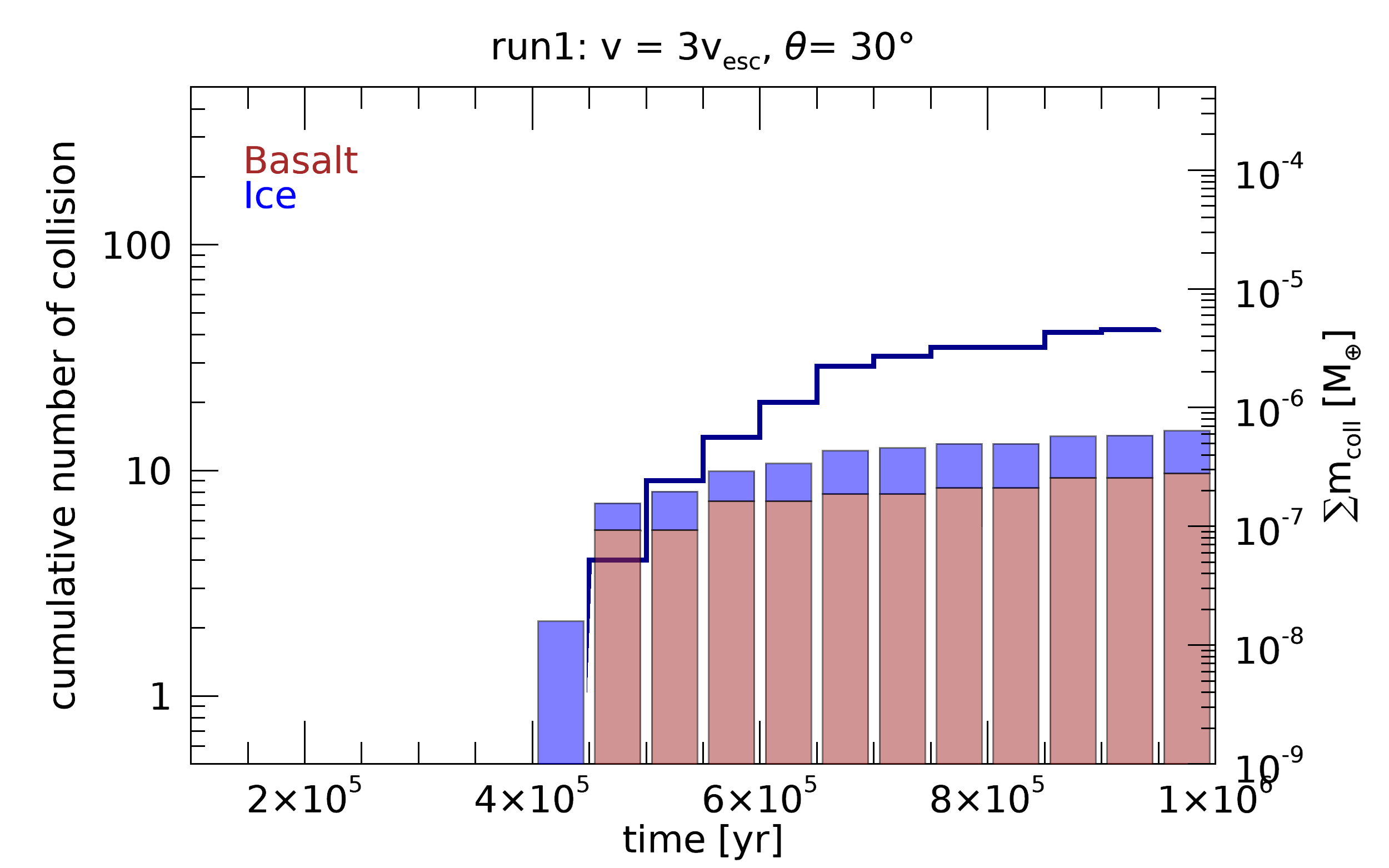
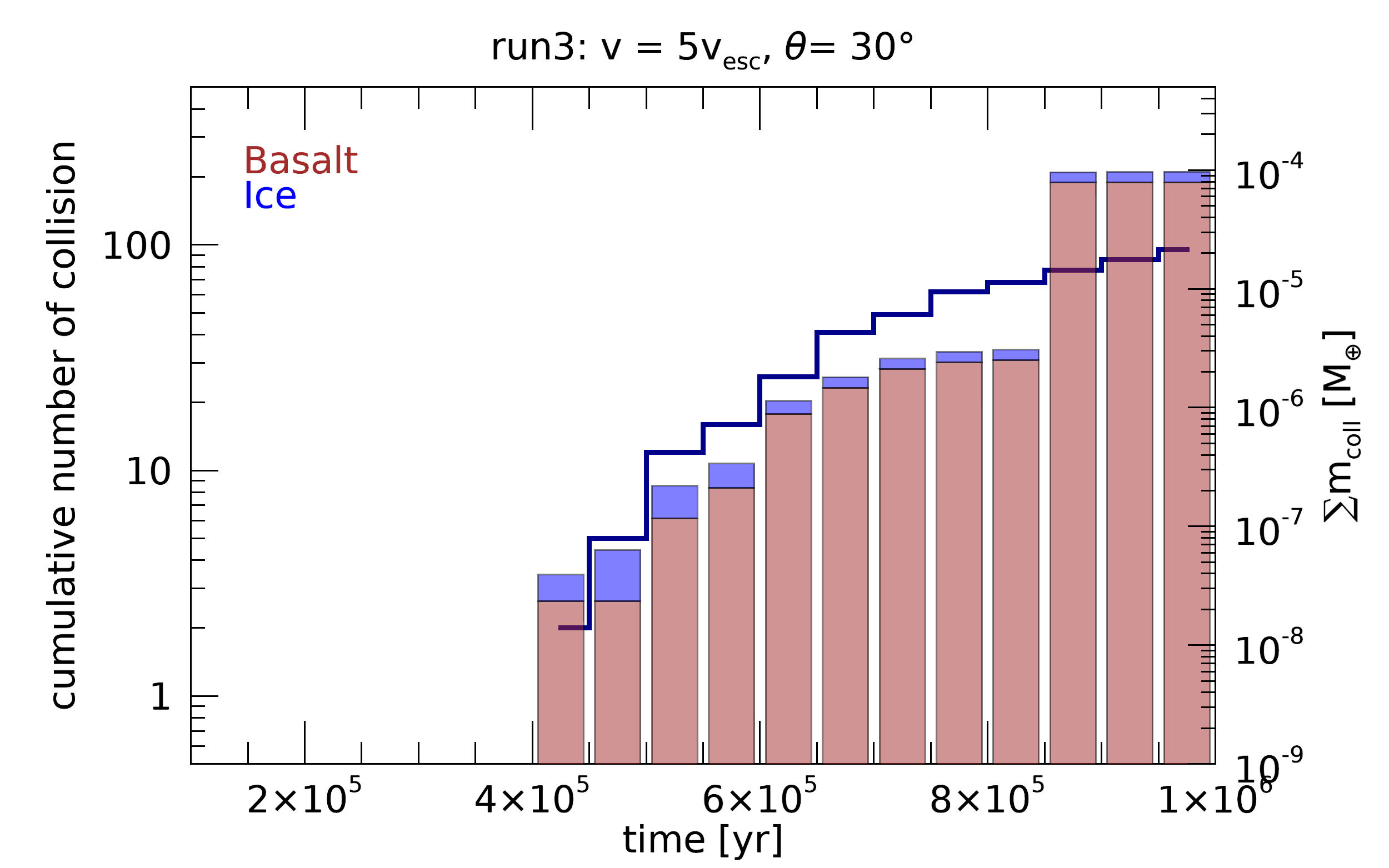
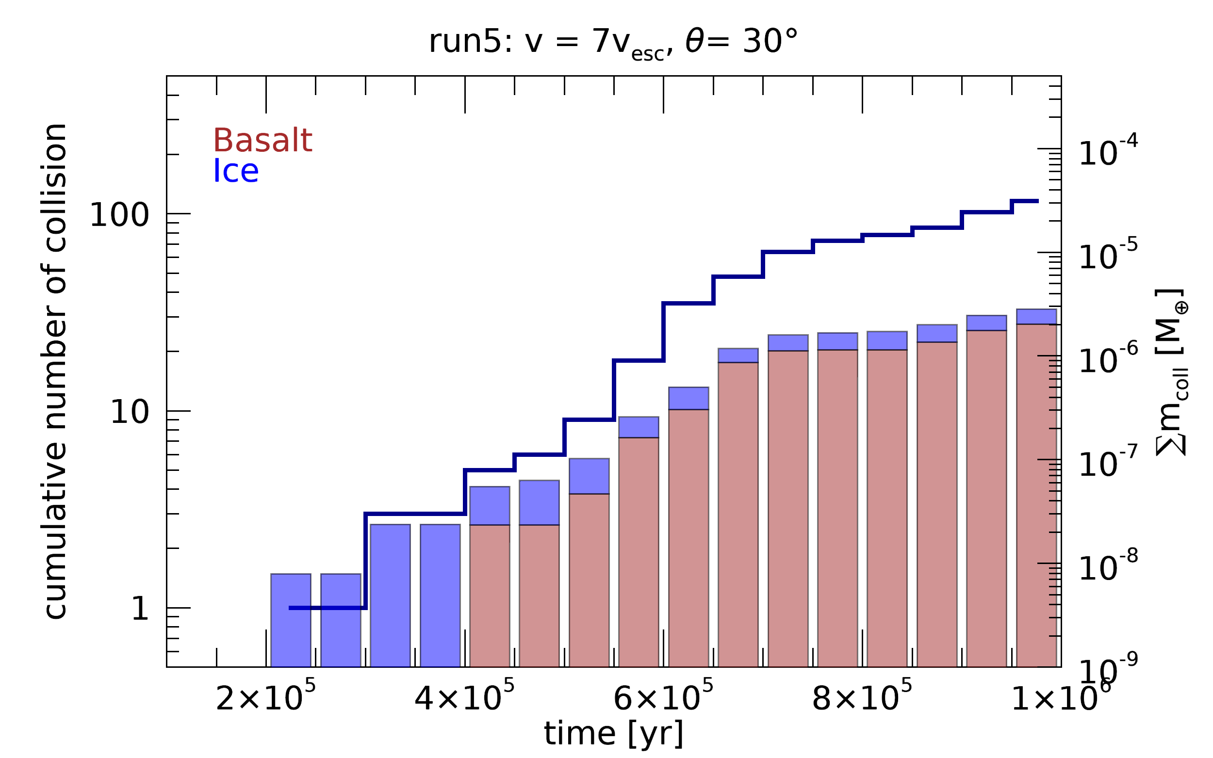
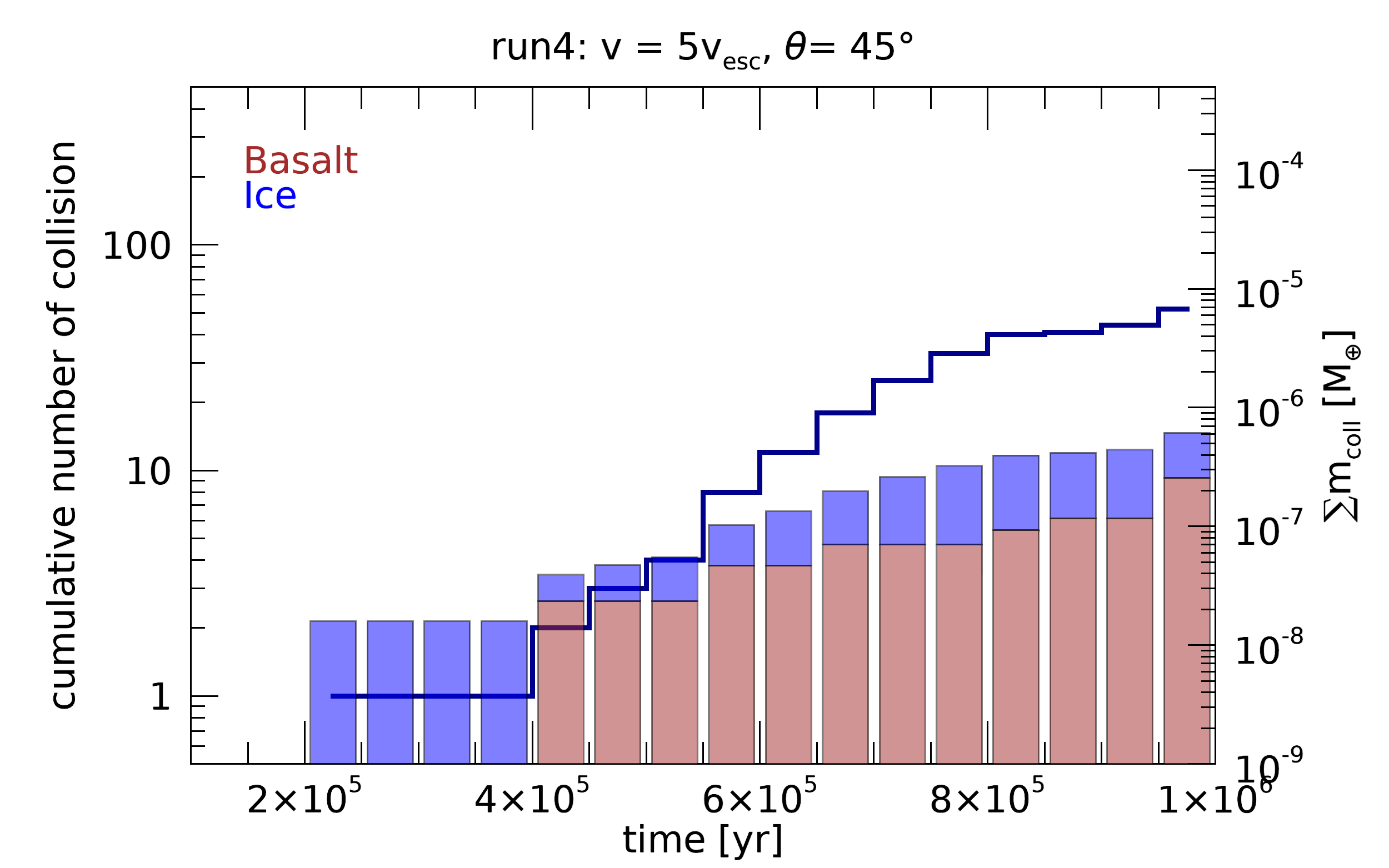
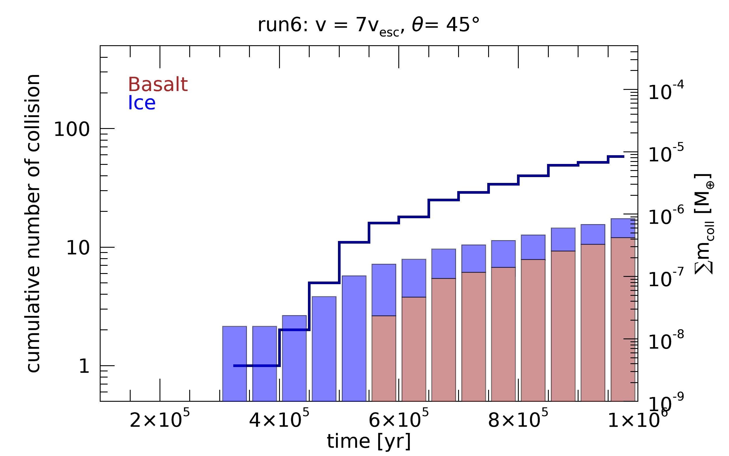
Figure 12: The event history of bodies colliding with the Earth. On the left axis, the cumulative number of bodies that collided with the Earth (blue line). On the right axis, the cumulative mass of bodies that collided with the Earth (brown and blue bars) in units of Earth-mass. The brown colour represents the amount of basalt in the total mass, while the blue colour represents water ice. Note that the horizontal axis begins at $t=10^{5}$ yr.

In Figure 12 the chronological record of collisions between fragments and Earth is shown. On the left hand the vertical axes shows the cumulative count of these collisions (blue line), while on the right hand axis the cumulative mass of the fragments are plotted. From the figure it is evident that initially smaller debris composed solely of pure water ice collide with the Earth. This typically begins around $\sim 2\cdot 10^{5}-4\cdot 10^{5}$ years after the impact event. Larger debris carrying both basalt and water ice, on the other hand, collide with the Earth later, around $\sim 4\cdot 10^{5}-6\cdot 10^{5}$ years after the impact.

Table 4: Maximum amount of water that may deliver to Earth from the asteroid belt. Columns 2 and 3 list $M_{\mathrm{wd}}$ as computed from Eq. (18) using $P$ from Table 3 for $f_{\mathrm{n}}=1$ and 3, respectively. Columns 4 and 5 are the same as Columns 2 and 3 but for $P^{\star}$. Column 6 presents $\Delta m_{\mathrm{ice}}$ as determined from impacts of fragments into the Earth using the results of the simulations (cf. Table 5).

Sim.	$M_{\mathrm{wd}}\,[\mathrm{M_{\mathrm{o}}}]$		$M_{\mathrm{wd}}^{\star}\,[\mathrm{M_{\mathrm{o}}}]$		$\Delta m_{\mathrm{ice}}\,[\mathrm{M_{\mathrm{o}}}]$
	$f_{\mathrm{n}}=1$	$f_{\mathrm{n}}=3$	$f_{\mathrm{n}}=1$	$f_{\mathrm{n}}=3$
run1	1.90	5.71	8.26	24.79	0.00142
run2	2.78	8.34	9.27	27.81	0.00098
run3	1.49	4.48	9.58	28.74	0.07093
run4	1.76	5.29	10.64	31.91	0.00142
run5	1.19	3.57	7.92	23.76	0.00322
run6	1.41	4.22	10.89	32.67	0.0017

According to Table 4 in most cases, the quantity of water delivered to Earth by the debris fluctuates around 0.001 ocean units, except for the run3 where more than 0.07 ’ocean’ of water is delivered. This means that as a result of a single distant collision, over 7% of the surface water is delivered to Earth. In this particular case, the remnants of the projectile collided with Earth, bringing along a significant amount of water (initially the projectile contained $\sim 0.16$ ’ocean’ of water). According to Morbidelli et al. (2000), the majority of the water currently present on Earth was delivered by a small number of planetary embryos that were initially formed in the outer asteroid belt and subsequently accreted by the Earth during its final stage of formation. The results of run3 are consistent with this finding. The special case of run3 is very well visible in Fig. 13 (green solid line), where the quantity of water transported to Earth, measured in terms of ocean units versus time is plotted for the 6 simulations. In general, the amount of water delivered to Earth initially increases rapidly, then the growth rate slows down and stabilizes at around 0.1%. An exception to this trend is observed in run3, as discussed earlier, when the remnants of the projectile hits the Earth at about $t\approx 8.7\cdot 10^{5}$ years, and depositing large quantity of water ice.

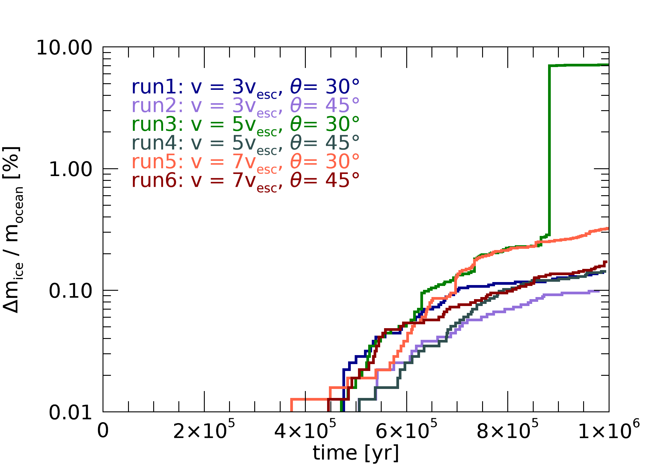
Figure 13: The amount of water delivered to Earth in ocean units over time in the 6 simulations. The run3 is a special case where the water is primarily delivered by the remnants of a single object, the remnant of the projectile, which collided with Earth at $t\approx 8.7\cdot 10^{5}$ years.

In Table 5 we have summarized the total mass delivered by impacts in all six simulations, along with its distribution specifically between basalt and water ice. Only the bodies that have participated in at least one collision are listed in the table. The second column provides information about the mass increase resulting from impacts. We can see that different bodies experience varying degrees of mass increase, with values spanning several orders of magnitude. Among the terrestrial planets Earth receives the highest amount of material, while Venus and Mars acquire negligible mass. The higher mass increase on the Earth could be attributed to various factors, predominantly its inflated size and gravitational attraction.

In all six runs the mass increase for the Sun is significantly higher compared to other bodies, ranging from $2.252\cdot 10^{19}$ kg to $1.897\cdot 10^{21}$ kg, depending on the specific run. Roughly half of the mass absorbed by the Sun consists of basalt, with the remaining half being water ice, but in all cases, the mass of basalt is greater. The number of collisions involving the Sun varies from 178 to 600, indicating a relatively high frequency of impacts compared to other bodies.

Generally the mass increase resulting from impacts is roughly the same for the Target and the Projectile in all scenarios, except two cases: In run1, the target accretes five times more mass than the projectile, while in run5, the post-projectile (pl7) accumulates three times more mass than the target. The number of collisions varies between the Target and Projectile. In some scenarios, the Target experiences a higher number of collisions, while in others, the Projectile has more collisions.

Overall, the data in the table provides insights into the effects of impacts on mass increase and collision occurrences for various bodies.

Table 5: Summary of the collisions with $R_{\mathrm{Earth}}=10R_{\oplus}$ for $T=10^{6}$ years for all six giant impacts. A specific object is only listed if it has suffered from a collision. The first column contains the names of the bodies. In the second column, the mass increase resulting from impacts is displayed in kg. In the third and fourth columns, this mass increase is specified for different materials, namely basalt and water ice. The fifth column shows the number of collisions (cf. it with the data in Table 2). In run5 both the target and the projectile disintegrate into smaller fragments, leaving no protoplanets but planetesimals pl6 and pl7.

Name	$\Delta m$ [kg]	$\Delta m_{\mathrm{Bas}}$ [kg]	$\Delta m_{\mathrm{ice}}$ [kg]	$N_{\mathrm{coll}}$
run1 $\left(v=3,\,\theta=30^{\circ}\right)$
Sun	5.525E19	3.921E19	1.604E19	178
Venus	1.395E17	1.395E17	0	1
Earth	3.802E18	1.673E18	2.129E18	47
Target	9.570E18	4.601E18	4.969E18	96
Projectile	5.214E19	3.879E19	1.335E19	114
run2 $\left(v=3,\,\theta=45^{\circ}\right)$
Sun	9.146E20	6.982E20	2.165E20	181
Earth	1.746E18	2.790E17	1.467E18	33
Target	5.259E18	2.230E18	3.028E18	52
Projectile	2.833E18	2.787E17	2.555E18	49
run3 $\left(v=5,\,\theta=30^{\circ}\right)$
Sun	6.352E20	5.137E20	1.215E20	427
Earth	5.790E20	4.725E20	1.064E20	95
Target	3.899E19	3.085E19	8.140E18	93
Projectile	2.380E19	1.633E19	7.477E18	115
run4 $\left(v=5,\,\theta=45^{\circ}\right)$
Sun	1.897E21	1.407E21	4.900E20	307
Earth	3.664E18	1.534E18	2.130E18	52
Jupiter	1.393E17	1.393E17	0	1
Target	4.931E18	2.092E18	2.839E18	66
Projectile	6.398E18	2.091E18	4.307E18	90
run5 $\left(v=7,\,\theta=30^{\circ}\right)$
Sun	1.279E+20	1.005E+20	2.735E+19	600
Earth	1.697E+19	1.214E+19	4.827E+18	116
Mars	1.866E+17	1.393E+17	4.729E+16	2
Jupiter	9.456E+16	0	9.456E+16	2
pl6	5.207E+19	4.303E+19	9.039E+18	71
pl7	1.422E+20	1.169E+20	2.527E+19	63
run6 $\left(v=7,\,\theta=45^{\circ}\right)$
Sun	2.252E19	1.311E19	9.417E18	245
Earth	5.066E18	2.510E18	2.556E18	58
Mars	9.458E16	0	9.458E16	2
Target	1.188E19	7.810E18	4.069E18	102
Projectile	1.659E19	1.158E19	5.016E18	97

4 Conclusions

The focus of this study is to examine the fate of debris ejected during collisions among celestial bodies in the asteroid belt and to study their role in the delivery of water to the Earth. In the applied model all major planets in the Solar System have already formed and are revolving around the Sun on their current orbits. To achieve our objective, we utilized SPH and $N$-body simulations to quantify the water transported to Earth through debris ejected from collisions between two Ceres-sized bodies near the $\nu_{6}$ secular resonance. We successfully combined the SPH code with the $N$-body simulator and provided a detailed description of generating initial conditions that lead to collisions at the desired location and velocity.

As a result of $N$-body simulations in the ($a-e$) planes (see Fig. 6), an intriguing checkmark-shaped pattern emerges at $t=0$ in all instances, encompassing both massive and massless bodies. In contract, in the distribution of bodies on the ($a-i$) plane (see Fig. 7) such a distinct structure is not as apparent. However, at higher collision velocities, two arc-like structures become evident in the distribution of planetesimals. The other type of fragments are dispersed around the impact site. It is clear that in the vicinity of the secular resonance, the ($a-e$) plane clears out, and the bodies end up on highly eccentric orbits (which is not visible in the figures because $e<0.25$). The $\nu_{6}$ secular resonance pumps up the eccentricities, and the highly elongated orbits intersect with the orbits of Mars and even Earth, allowing for impacts on these rocky planets. In Figs. 8 and 9, the extent and shape of the $\nu_{6}$ secular resonance are clearly visible from the distribution of objects that collided with Earth during the simulations.

After the collision, the created the check-mark-shaped pattern’s extension along the semi-major axis, increases with velocity $v$. At $v=3$, it spans more than 0.5 au, while at $v=7$, it covers nearly 1 au in width. Consequently, if a collision deviates from the location of the $\nu_{6}$ secular resonance by no more than 0.5 au, due to the scattering effect, debris will enter the resonance. The quantity of debris that enters depends on the distance and velocity of the collision. Since collisions are frequent in the early stages of planetary formation, it’s likely that the $\nu_{6}$ resonance receives a continuous supply, which it then "transmits" to the inner regions through the mechanism outlined above. From the perspective of the inner planets, this represents a continuous water delivery system that persists as long as there are collisions and debris enters the resonance.

Based on the data from the $N$-body simulations, we calculated the probability of the ejected debris impacting Earth. Using this information, we provided an upper estimate for the amount of water that can be transported by the debris. Considering the significant uncertainties and strong model dependencies, our estimate is in reasonable agreement with previous results, such as ML and Morbidelli et al. (2000). According to our findings, a minimum of $\approx 1.2$ and a maximum of $\approx 2.8$ ocean equivalents of water can be delivered if the MMSN model is considered. However, if we assume an equivalent mass of 3 $\times$ MMSN of solids and calculate the water quantity, the range increases to 3.6 to 8.3 ocean equivalents, indicating the potential delivery of larger amounts of water to Earth. Therefore, if the total water inventory on Earth is estimated to be between 1 and 10 ocean equivalents, the external pollution model can provide an explanation for Earth’s total water inventory. If this is true, it would not require assuming local sources to explain the origin of water, although they cannot be ruled out either.

During the $N$-body simulations, we were able to directly measure the amount of water brought to Earth by the ejected debris during individual collisions. Typically, this amounted to 0.001 ocean equivalents of water. An interesting exception was observed when a single large body, the remnants of the projectile, collided with Earth and deposited approximately 0.07 ocean equivalents of water on the Earth’s surface. The results of this study support the widely accepted external pollution model. The maximum estimated amount of water that was transported to the Earth via fragments varies between 1.2 and 8.3 ocean’s worth, depending on the initial mass of the protoplanetary disk.

Data Availability

The data underlying this paper will be shared on reasonable request to the authors.

References

- Abe et al. (2000) Abe Y., Ohtani E., Okuchi T., Righter K., Drake M., 2000, in Canup R. M., Righter K., et al. eds, , Origin of the Earth and Moon. pp 413–433
- Alexander et al. (2012) Alexander C. M. O., Bowden R., Fogel M. L., Howard K. T., Herd C. D. K., Nittler L. R., 2012, Science, 337, 721
- Benz & Asphaug (1995) Benz W., Asphaug E., 1995, Computer Physics Communications, 87, 253
- Bottke et al. (2000) Bottke William F. J., Rubincam D. P., Burns J. A., 2000, Icarus, 145, 301
- Bottke et al. (2002) Bottke W. F., Morbidelli A., Jedicke R., Petit J.-M., Levison H. F., Michel P., Metcalfe T. S., 2002, Icarus, 156, 399
- DeMeo & Carry (2014) DeMeo F. E., Carry B., 2014, Nature, 505, 629
- Dormand & Prince (1978) Dormand J. R., Prince P. J., 1978, Celestial Mechanics, 18, 223
- Fogg & Nelson (2005) Fogg M. J., Nelson R. P., 2005, A&A, 441, 791
- Fogg & Nelson (2007) Fogg M. J., Nelson R. P., 2007, A&A, 461, 1195
- Forgács-Dajka et al. (2022) Forgács-Dajka E., Sándor Z., Sztakovics J., 2022, A&A, 657, A135
- Froeschle & Scholl (1986) Froeschle C., Scholl H., 1986, A&A, 166, 326
- Genda et al. (2012) Genda H., Kokubo E., Ida S., 2012, ApJ, 744, 137
- Gingold & Monaghan (1977) Gingold R. A., Monaghan J. J., 1977, MNRAS, 181, 375
- Gradie & Tedesco (1982) Gradie J., Tedesco E., 1982, Science, 216, 1405
- Hayashi (1981) Hayashi C., 1981, Progress of Theoretical Physics Supplement, 70, 35
- Héder et al. (2022) Héder M., et al., 2022, Információs Társadalom, 22, 128
- Hirschmann (2006) Hirschmann M. M., 2006, Annual Review of Earth and Planetary Sciences, 34, 629
- Ito & Malhotra (2006) Ito T., Malhotra R., 2006, Advances in Space Research, 38, 817
- Kerridge (1985) Kerridge J. F., 1985, Geochimica Cosmochimica Acta, 49, 1707
- Knezevic et al. (1991) Knezevic Z., Milani A., Farinella P., Froeschle C., Froeschle C., 1991, Icarus, 93, 316
- Kokubo & Ida (2000) Kokubo E., Ida S., 2000, Icarus, 143, 15
- Krasinsky et al. (2002) Krasinsky G. A., Pitjeva E. V., Vasilyev M. V., Yagudina E. I., 2002, Icarus, 158, 98
- Kuchynka & Folkner (2013) Kuchynka P., Folkner W. M., 2013, Icarus, 222, 243
- Kővári et al. (2023) Kővári E., Forgács-Dajka E., Kovács T., Kiss C., Sándor Z., 2023, A dynamical survey of the trans-Neptunian region II.: On the nature of chaotic diffusion (arXiv:2305.19018)
- Maindl & Dvorak (2014) Maindl T. I., Dvorak R., 2014, in Exploring the Formation and Evolution of Planetary Systems. pp 370–373 (arXiv:1307.1643), doi:10.1017/S1743921313008971
- Maindl & Haghighipour (2014) Maindl T. I., Haghighipour N., 2014, in AAS/Division for Planetary Sciences Meeting Abstracts #46. p. 415.17
- Maindl et al. (2013) Maindl T. I., Schäfer C., Speith R., Süli Á., Forgács-Dajka E., Dvorak R., 2013, Astronomische Nachrichten, 334, 996
- Maindl et al. (2014) Maindl T. I., Dvorak R., Schäfer C., Speith R., 2014, in Complex Planetary Systems, Proceedings of the International Astronomical Union. pp 138–141 (arXiv:1409.2298), doi:10.1017/S1743921314008059
- Maindl et al. (2015) Maindl T. I., et al., 2015, A&A, 574, A22
- Martin & Livio (2021) Martin R. G., Livio M., 2021, MNRAS, 506, L6
- Marty (2006) Marty B., 2006, Reviews in Mineralogy and Geochemistry, 62, 421
- Marty (2012) Marty B., 2012, Earth and Planetary Science Letters, 313, 56
- Minton & Malhotra (2011) Minton D. A., Malhotra R., 2011, ApJ, 732, 53
- Morbidelli & Henrard (1991) Morbidelli A., Henrard J., 1991, Celestial Mechanics and Dynamical Astronomy, 51, 169
- Morbidelli et al. (1994) Morbidelli A., Gonczi R., Froeschle C., Farinella P., 1994, A&A, 282, 955
- Morbidelli et al. (2000) Morbidelli A., Chambers J., Lunine J. I., Petit J. M., Robert F., Valsecchi G. B., Cyr K. E., 2000, Meteoritics and Planetary Science, 35, 1309
- Nobili et al. (1989) Nobili A. M., Milani A., Carpino M., 1989, A&A, 210, 313
- Raymond & Izidoro (2017) Raymond S. N., Izidoro A., 2017, Icarus, 297, 134
- Raymond & Morbidelli (2022) Raymond S. N., Morbidelli A., 2022, in Biazzo K., Bozza V., Mancini L., Sozzetti A., eds, Astrophysics and Space Science Library Vol. 466, Demographics of Exoplanetary Systems, Lecture Notes of the 3rd Advanced School on Exoplanetary Science. pp 3–82 (arXiv:2002.05756), doi:10.1007/978-3-030-88124-5_1
- Raymond et al. (2005) Raymond S. N., Quinn T., Lunine J. I., 2005, ApJ, 632, 670
- Schäfer (2005) Schäfer C., 2005, PhD thesis, Eberhard Karls University of Tubingen, Germany
- Schäfer et al. (2020) Schäfer C. M., et al., 2020, Astronomy and Computing, 33, 100410
- Scholl & Froeschle (1991) Scholl H., Froeschle C., 1991, A&A, 245, 316
- Smallwood et al. (2018) Smallwood J. L., Martin R. G., Lepp S., Livio M., 2018, MNRAS, 473, 295
- Süli (2021) Süli Á., 2021, MNRAS, 503, 4700
- Thomas et al. (2005) Thomas P. C., Parker J. W., McFadden L. A., Russell C. T., Stern S. A., Sykes M. V., Young E. F., 2005, Nature, 437, 224
- Warner et al. (2009) Warner B. D., Harris A. W., Vokrouhlický D., Nesvorný D., Bottke W. F., 2009, Icarus, 204, 172
- Weidenschilling (1977) Weidenschilling S. J., 1977, Ap&SS, 51, 153
- Yoshikawa (1987) Yoshikawa M., 1987, Celestial Mechanics, 40, 233