Revisiting Transferable Adversarial Image Examples:
Attack Categorization, Evaluation Guidelines, and New Insights

Abstract

Transferable adversarial examples raise critical security concerns in real-world, black-box attack scenarios. However, in this work, we identify two main problems in common evaluation practices: (1) For attack transferability, lack of systematic, one-to-one attack comparison and fair hyperparameter settings. (2) For attack stealthiness, simply no comparisons. To address these problems, we establish new evaluation guidelines by (1) proposing a novel attack categorization strategy and conducting systematic and fair intra-category analyses on transferability, and (2) considering diverse imperceptibility metrics and finer-grained stealthiness characteristics from the perspective of attack traceback. To this end, we provide the first large-scale evaluation of transferable adversarial examples on ImageNet, involving 23 representative attacks against 9 representative defenses.

Our evaluation leads to a number of new insights, including consensus-challenging ones: (1) Under a fair attack hyperparameter setting, one early attack method, DI, actually outperforms all the follow-up methods. (2) A state-of-the-art defense, DiffPure, actually gives a false sense of (white-box) security since it is indeed largely bypassed by our (black-box) transferable attacks. (3) Even when all attacks are bounded by the same $L_{p}$ norm, they lead to dramatically different stealthiness performance, which negatively correlates with their transferability performance. Overall, our work demonstrates that existing problematic evaluations have indeed caused misleading conclusions and missing points, and as a result, hindered the assessment of the actual progress in this field. Code is available at https://github.com/ZhengyuZhao/TransferAttackEval.

1 Introduction

Deep Neural Networks (DNNs) have achieved great success in various machine learning tasks. However, they are known to be vulnerable to adversarial examples [19, 68], which are intentionally perturbed model inputs to induce prediction errors. Adversarial examples have been studied in the white-box scenario to explore the worst-case model robustness but also in the black-box scenario to understand the real-world threats to deployed models.

An intriguing property of adversarial examples that makes them threatening in the real world is their transferability. Transferable attacks assume a realistic scenario the adversarial examples generated on a (local) surrogate model can be directly transferred to the (unknown) target model [52, 39]. Such attacks require no “bad” query [12] interaction with the target model, and as a result, they eliminate the possibility of being easily flagged by the target model under attack [10]. Due to their real-world implications, transferable attacks have attracted great attention, and an increasing number of new methods have been rapidly developed. However, we identify two major problems in common evaluation practices.

Table 1: Evaluation practices in existing work compared to ours in terms of attack transferability and stealthiness.

Evaluation	Transferability	Stealthiness
Existing	Unsystematic: Indiscriminate comparisons ✗	Pre-fixed $L_{\infty}$ norm without any comparison ✗
	“New+Old vs. Old” (half the time) ✗
	Unfair: Inconsistent hyperparameter settings for similar attacks ✗
	Limited hyperparameter tuning ✗
Our	Systematic: Intra-/inter-category comparisons ✓	Pre-fixed $L_{\infty}$ norm with diverse comparisons ✓
	“New vs. Old” by isolating the core of each attack ✓	(1) Five popular imperceptibility metrics
	Fair: Consistent intra-category hyperparameter settings ✓	(2) Two new fine-grained stealthiness measures
	Hyperparameter tuning based on intra-category analyses ✓	from the perspective of attack traceback

Problem 1. Existing evaluations are often unsystematic and sometimes unfair. When a new attack is compared to an old attack, it is often compared following “New+Old vs. Old” instead of “New vs. Old”. As can be seen from Table 11 in Appendix B, half of existing studies have such a problem. In general, “New+Old vs. Old” only reflects the additive value of “New” to “Old”, which is somewhat expected given the additional efforts made by “New”. However, especially when both attacks fall into the same category, “New vs. Old” is required for achieving a meaningful comparison. For example, although both DI [86] and TI [15] are based on input augmentations, the original work of TI only considers “TI+DI vs. TI” but whether or not TI is better than DI is unknown. Moreover, in some cases, unfair hyperparameter settings are adopted (even when “New vs. Old” is followed). Specifically, among existing input augmentation-based attacks, the relatively new methods (i.e., Admix [73], SI [38], and VT [72]) adopt multiple input copies for their new methods but only one input copy for earlier attacks (i.e., DI [86] and TI [15]).

Problem 2. Existing evaluations solely compare attack strength, i.e., transferability, but largely overlook another key attack property, stealthiness. Instead, they pre-fix the stealthiness based on simply imposing a single $L_{p}$ norm on the perturbations. This is problematic since it is well known that a successful attack requires a good trade-off between attack strength and stealthiness. More generally, (black-box) transferable attacks normally require larger perturbations than white-box attacks for success, but using a single $L_{p}$ norm is known to be insufficient when perturbations are not very small [62, 69]. In the context of transferable attacks, one recent study [9] also notices that the transferability of attacks bounded by the same $L_{\infty}$ norm is surprisingly correlated with their $L_{2}$ norms. In addition, other stealthiness measures beyond the image distance have not been explored.

Evaluation guidelines. We aim to address the above two problems by establishing new evaluation guidelines from both the perspectives of transferability and stealthiness. To address Problem 1, we propose a new categorization of existing transferable attacks (Section 2), which enables our systematic intra-category attack analyses (Section 4). Such analyses also provide support for attack hyperparameter selection, ensuring the fairness of our later comprehensive evaluations, which further involve inter-category comparisons (Section 5). To address Problem 2, we consider diverse stealthiness measures. Specifically, we adopt five different imperceptibility metrics beyond the $L_{p}$ norms. Moreover, we move beyond imperceptibility and investigate other aspects of stealthiness, such as attack traceback based on (input) image features or (output) misclassification features. Table 1 summarizes our good evaluation practices compared to those in existing work in terms of attack transferability and stealthiness.

Overall, we present the first large-scale evaluation of transferable adversarial examples, testing 23 representative transferable attacks (in 5 categories) against 9 representative defenses (in 3 categories) on 5000 ImageNet images. These attacks and defenses have been published in the past 5 years (i.e., 2018-2023) at top-tier security and machine learning conferences (NDSS, ICLR, ICML, NeurIPS, CVPR, ICCV, ECCV, etc.), and they can represent the current state of the art in transferable adversarial examples. In comparison, existing work considers 11 attacks at most, as summarized by Table 11 in Appendix B. A recent study [45] has also provided a large-scale evaluation of attack transferability. However, it actually only considers conventional attacks (e.g., FGSM, CW, and DeepFool), which were published before 2017. In addition, it focuses on attacking private cloud-based MLaaS platforms instead of public models.

Our evaluation leads to new insights that complement or even challenge existing knowledge about transferable attacks. In sum, these insights suggest that our identified evaluation problems in existing work have indeed led to misleading conclusions and missing points, making the actual progress of transferable attacks hard to assess.

New insights into transferability. In general, we find that the performance of different methods is highly contextual, i.e., the optimal (category of) attack/defense for one (category of) defense/attack may not be optimal for another. In particular, we reveal that a defense may largely overfit specific attacks that generate adversarial examples similar to those used in the optimization of that defense. For example, DiffPure [51] claims the state-of-the-art white-box robustness and even beats adversarial training [44] in their original evaluation. On the contrary, we demonstrate that DiffPure is surprisingly vulnerable to (black-box) transferable attacks that produce semantic perturbations (within the claimed norm bounds). See Section 5 for detailed results. Our intra-category attack analyses also lead to surprising findings regarding transferability. For example, for gradient stabilization attacks, using more iterations may even decrease the performance. Another example is that the earliest input augmentation-based attack, DI, actually outperforms all subsequent attacks when they are compared fairly with the same number of input copies.

New insights into stealthiness. In general, we find that stealthiness may be at odds with transferability. Specifically, almost all transferable attacks yield worse imperceptibility than the PGD baseline, in terms of five imperceptibility metrics. This suggests that it is problematic to solely constrain all attacks with the same $L_{\infty}$ norm bound without more comprehensive comparisons. Moreover, different attacks yield dramatically different stealthiness characteristics, in terms of imperceptibility and other aspects. For example, the adversarial images generated from different attacks are well separable solely based on their visual features. In addition, different attacks lead to different misclassification patterns regarding the model output distribution. These new explorations suggest the possibility of  “attack traceback” based on (input) image features or (output) misclassification features.

2 Attack Categorization

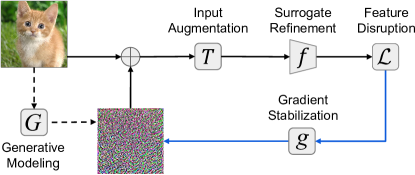
Figure 1: Illustration of our attack categorization along with the common pipeline of iterative attacks. Note that the generative modeling attack is independent. $T$: transformation, $f$: model, $\mathcal{L}$: loss, $g$: gradient, $G$: generator.

In this section, we introduce our new categorization of transferable attacks. First of all, these attacks can be generally divided into two types: iterative and generative attacks. For iterative attacks, we derive four categories: gradient stabilization, input augmentation, feature disruption, and surrogate refinement. Each of these four categories operates on one of the four major components in the common pipeline of iterative attacks: gradient, (image) input, (loss) output, and (surrogate) model. The relation between these four categories and the pipeline is illustrated in Figure 1. Due to the specific nature of generative attacks, we leave it as an independent category: generative modeling.

In general, these five categories are disjoint to each other, i.e., each attack falls into only one category according to the technique that was claimed as the key contribution in its original work. Different attack methods that share the same key idea fall into the same category and can be compared systematically in a single dimension. Table 2 summarizes the key ideas of the five categories. Our new attack categorization is also suggested to be reliable based on a perturbation classification task (see Section 5.2). Note that our categorization does not involve ensemble attacks [39, 35] since they can be integrated with any attack.

In the following, we present these five categories in turn. Before that, we briefly formulate the optimization process of adversarial attacks in image classification. Given a classifier $f(\mathbf{x}):\mathbf{x}\in\mathcal{X}\to y\in\mathcal{Y}$ that predicts a label $y$ for an original image $\mathbf{x}$, an attacker aims to create an adversarial image $\mathbf{x}^{\prime}$ by perturbing $\mathbf{x}$. For iterative attacks, which fall into our first four categories, the adversarial image is iteratively optimized based on gradients:

$$\mathbf{x}^{\prime}_{0}=\mathbf{x},~{}\mathbf{x}^{\prime}_{i+1}=\mathbf{x}^{\prime}_{i}+\eta\cdot\mathrm{sign}(\mathbf{g}_{i}),~{}\textrm{where}~{}\mathbf{g}_{i}=\nabla_{\mathbf{x}}\mathcal{L}.$$ (1)

Here, $\mathbf{x}^{\prime}_{i}$ is the intermediate adversarial image at the $i$-th iteration, $\mathbf{g}_{i}$ is the intermediate gradient vector, and $\mathcal{L}$ is the adversarial loss function. In order to speed up the optimization and ensure the image is in the original quantized domain (e.g., with 8-bit), a sign operation is commonly added to keep only the direction of the gradients but not their magnitude [19].

Specifically, the gradient calculation in the baseline attack, PGD [31, 44], can be formulated as follows:

$$\mathbf{g}_{i}=\nabla_{\mathbf{x}}\mathcal{L}_{CE}(\mathbf{x}^{\prime}_{i},y,f),$$ (2)

where the loss function $\mathcal{L}_{CE}$ is the cross-entropy loss, which takes as inputs the image, label, and model. In each of the following four attack categories, only one of the four major components (i.e., gradient update, input, loss function, and model) in Equation 2 would be modified.

2.1 Gradient Stabilization

Different DNN architectures tend to yield radically different decision boundaries, yet similar test accuracy, due to their high non-linearity [39, 64]. For this reason, the attack gradients calculated on a specific (source) model may cause the adversarial images to trap into local optima, resulting in low transferability to a different (target) model. To address this issue, popular machine learning techniques that can stabilize the update directions and help the optimization escape from poor local maxima during the iterations are useful. Existing work on transferable attacks has adopted two such techniques, momentum [54] and Nesterov accelerated gradient (NAG) [50], by adding a corresponding term into the attack optimization.

Table 2: Key ideas of different attack categories.

Attack Categories	Key Ideas
Gradient Stabilization	Stabilize the gradient update
Input Augmentation	Augment the input image
Feature Disruption	Disrupt intermediate-layer features
Surrogate Refinement	Refine the surrogate model
Generative Modeling	Learn a perturbation generator

In this way, the attack is optimized based on gradients from not only the current iteration but also other iteration(s) determined by the additional term. Specifically, the momentum is to accumulate previous gradients, i.e., looking back [14], and the Nesterov accelerated gradient (NAG) is an improved momentum that additionally accumulates future gradients, i.e., looking ahead [38]. In particular, NAG is later examined in [74], where using only the single previous gradient for looking ahead is found to work better than using all previous gradients. In terms of the formulation, the gradient calculation in Equation 2 becomes:

$$\begin{split}&\textrm{MI~{}\cite[cite]{[\@@bibref{}{dong2018boosting}{}{}]}:}~{}\mathbf{g}_{i}=\mu\cdot\mathbf{g}_{i-1}+\nabla_{\mathbf{x}}\mathcal{L}_{CE}(\mathbf{x}^{\prime}_{i},y,f),\\ &\textrm{NI~{}\cite[cite]{[\@@bibref{}{lin2020nesterov}{}{}]}:}~{}\mathbf{g}_{i}=\mu\cdot\mathbf{g}_{i-1}+\nabla_{\mathbf{x}}\mathcal{L}_{CE}(\mathbf{x}^{\prime}_{i}+\alpha\cdot\mathbf{g}_{i-1},y,f),\\ &\textrm{PI~{}\cite[cite]{[\@@bibref{}{wang2021boosting}{}{}]}:}~{}\mathbf{g}_{i}=\mu\cdot\mathbf{g}_{i-1}+\nabla_{\mathbf{x}}\mathcal{L}_{CE}(\mathbf{x}^{\prime}_{i}+\alpha\cdot\nabla_{\mathbf{x}}\mathcal{L}_{CE}(\mathbf{x}^{\prime}_{i-1},y,f),y,f),\end{split}$$ (3)

where the first, momentum term in each equation is for looking back, and the second is for looking ahead.

2.2 Input Augmentation

Machine learning is a process where a model is optimized on a local dataset such that it can generalize to unseen test images. Following the same principle, learning transferable attacks can be treated as a process where an adversarial image is optimized on a local surrogate model such that it can generalize/transfer to unseen target models [36]. Due to this conceptual similarity, various techniques that are used for improving model generalizability can be exploited to improve attack transferability. Data augmentation is one such technique that is commonly explored in existing work on transferable attacks. To this end, the adversarial images are optimized to be invariant to a specific image transformation. In terms of the formulation, the gradient calculation in Equation 2 becomes:

$$\mathbf{g}_{i}=\nabla_{\mathbf{x}}\mathcal{L}_{CE}(T(\mathbf{x}^{\prime}_{i}),y,f),$$ (4)

where the input image is first transformed by a specific image transformation $T$.

According to the idea of data augmentation, the transformation is required to be sematic-preserving. For example, in image classification, a transformed image should still be correctly classified. Existing work has explored various types of image transformations, such as geometric transformations (e.g., resizing & padding [86] and translation [15]), pixel value scaling [38], random noise [72], and mixing images from incorrect classes [73]. Recent studies also explore more complex methods that refine the above transformations [106, 91], leverage regional (object) information [34, 5, 79], or rely on frequency-domain image transformations [41].

2.3 Feature Disruption

It is understandable that adversarial attacks in image classification commonly adopt cross-entropy loss because this loss is also used for classification by default. However, this choice may not be optimal for transferable attacks since the output-layer, class information is often model-specific. In contrast, features extracted from the intermediate layers are known to be more generic [90, 30]. Based on this finding, existing work on transferable attacks has proposed to replace the commonly used cross-entropy loss with some feature-based loss. These studies aim to disrupt the feature space of an image such that the final class prediction would change. Specifically, the distance between the adversarial image and its corresponding original image in the feature space is maximized. In terms of the formulation, the gradient calculation in Equation 2 becomes:

$$\mathbf{g}_{i}=\nabla_{\mathbf{x}}d(f_{l}(\mathbf{x}^{\prime}_{i}),f_{l}(\mathbf{x}))$$ (5)

where $f_{l}$ calculates the feature output at a specific intermediate layer $l$ of the classifier, and $d(\cdot,\cdot)$ calculates the feature difference between the original and adversarial images.

Early methods of feature disruption attacks simply adopt the $L_{2}$ distance for $d(\cdot,\cdot)$ [49, 104, 17, 23, 40, 33]. In this way, the resulting feature disruption is indiscriminate at any image location. However, these methods are sub-optimal because the model decision normally only depends on a small set of important features [103]. To address this limitation, later methods [82, 76, 97] instead calculate the feature difference $d(\cdot,\cdot)$ based on only important features. In this case, the importance of different features is normally determined based on model interpretability results [60, 66]. Feature disruption is also explored for the relatively challenging, targeted attacks. In this case, rather than maximizing the distance between the original image and the adversarial image, the attack minimizes the distance between the original image and a target image [27] or a target distribution determined by a set of target images [25, 26]. Beyond feature disruption, other losses are also explored specifically for targeted attacks, such as the triplet loss [32] or logit loss [101].

2.4 Surrogate Refinement

The current CNN models are commonly learned towards high prediction accuracy but with much less attention given to transferable representations. Several recent studies find that adversarial training could yield a model that better transfers to downstream tasks, although it inevitably trades off the accuracy of a standard model in the source domain [58, 13, 71]. This finding encourages researchers to explore how to refine the surrogate model to improve the transferability of attacks. In terms of the formulation, the gradient calculation in Equation 2 becomes:

$$\mathbf{g}_{i}=\nabla_{\mathbf{x}}\mathcal{L}_{CE}(T(\mathbf{x}^{\prime}_{i}),y,f^{\prime}),$$ (6)

where $f^{\prime}$ demotes a refined version of the original model $f$.

The underlying assumption of surrogate refinement is a smooth surrogate model leads to transferable adversarial images. To this end, existing studies have explored three different ways, in which a standard model is modified in terms of training procedures [65, 94, 88] and architectural designs [20, 81, 93, 105]. Specifically, in terms of training procedures, using an adversarially-trained surrogate model is helpful since robust features are known to be smoother than non-robust features [24]. Similarly, early stopping [94] or training with soft annotations [88] are also shown to yield a smoother model. In terms of architectural designs, it is helpful to replace the non-linear, ReLU activation function with a smoother one [20, 93, 105]. For ResNet-like architectures, backpropagating gradients through skip connections is shown to result in higher transferability than through residual modules [81]. This line of research also leads to rethinking the relation between the accuracy of the surrogate model and the transferability [94, 105].

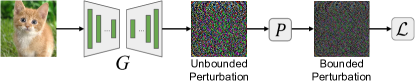
Figure 2: Illustration of the pipeline of generative modeling attacks. $G$: generator, $P$: projection, $\mathcal{L}$: loss.

2.5 Generative Modeling

In addition to the above iterative attacks, existing work also relies on Generative Adversarial Networks (GANs) [18] to directly generate transferable adversarial images. Generative modeling attacks can efficiently generate perturbations for any given image with only one forward pass. The GAN framework consists of two networks: a generator and a discriminator. The generator captures the data distribution, and the discriminator estimates the probability that a sample came from the training data rather than the generator. In the typical GAN training, these two networks are simultaneously trained in a minimax two-player game.

In the context of adversarial attacks, GAN is trained on additional (clean) data, and a pre-trained image classifier is adopted as the discriminator. Different from the typical GAN training, only the generator is updated but the discriminator is fixed. The training objective of the generator is to cause the discriminator to misclassify the generated image. A clipping operation is normally applied after the generation to constrain the perturbation size. Specifically, the perturbations output from the generator are initially unbounded and then clipped by a specific norm bound. This means that once trained, the generator can be used to generate perturbations under various constraints. The whole pipeline is illustrated in Figure 2.

Existing studies have explored different loss functions and architectures of the generator. Specifically, the earliest generative attack [55] adopts the widely-used cross-entropy loss. Later studies improve it by adopting a relativistic cross-entropy loss [48] or intermediate-level, feature losses [29, 98]. In particular, to improve targeted transferability, class-specific [47] and class-conditional [89] generators are also explored.

Table 3: Threat models considered in existing work regarding five aspects. For each aspect (A/B),   denotes only considering A,   denotes only considering B, and   denotes both.

Attacks	Scenario (public model/ private system)	Attack goal (untarget/ target)	Task (ImageNet/ others)	Model (CNNs/ others)	Source/target training data (same/ disjoint)
MI [14]
NI [38]
PI [74]
DI [86]
TI [15]
SI [38]
VT [72]
Admix [73]
TAP [104]
AA [27]
ILA [23]
FIA [76]
NAA [97]
SGM [81]
LinBP [20]
RFA [65]
IAA [105]
DSM [88]
GAP [55]
CDA [48]
GAPF [29]
BIA [98]
TTP [47]
Ours

3 Evaluation Methodology

In this section, we describe our evaluation methodology in terms of the threat model, evaluation metrics, and experimental setups.

3.1 Threat Model

Following the common practice, we specify our threat model from three dimensions: attacker’s knowledge, attacker’s goal, and attacker’s capability [53, 4, 6]. In general, we make sure our threat model follows the most common settings in existing work regarding five aspects, as summarized in Table 3.

Attacker’s knowledge. An attacker can have various levels of knowledge about the target model. In the ideal, white-box case, an attacker has full control over the target model. In the realistic, black-box case, an attacker has either query access to the target model or in our transfer setting, no access but only leverages a surrogate model. In this work, we follow most existing work to explore the attack transferability between image classifiers that are trained on the same public dataset (here ImageNet) but with different architectures. Cross-dataset transferability is rarely explored [48, 98] and beyond the scope of this work.

Attacker’s goal. Normally, an attacker aims at either untargeted or targeted misclassification. An untargeted attack aims to fool the classifier into predicting any other class than the original one, i.e., $f(\mathbf{x}^{\prime})\neq{y}$. A targeted attack aims at a specific incorrect class $t$, i.e., $f(\mathbf{x}^{\prime})=t$. Achieving the targeted goal is strictly more challenging because a specific (target) direction is required, while many (including random) directions suffice for untargeted success. Targeted success and non-targeted success follow fundamentally different mechanisms. Specifically, targeted success requires representation learning of the target class while untargeted success is relevant to model invariance to small noise [47, 101]. Technically, an untargeted attack is equal to running a targeted attack for each possible target and taking the closest [7]. In this work, we follow most existing work to focus on untargeted transferability since achieving the more challenging, targeted transferability remains an open problem [48, 47, 101]. The only place where we test targeted transferability is our new finding of the “early stopping” phenomenon for gradient stabilization attacks (See Section 4.1).

Attacker’s capability. In addition to the adversarial effects, an attack should be constrained to stay stealthy. Most existing work addresses this by pursuing the imperceptibility of perturbations, based on the simple, $L_{p}$ norms [7, 19, 31, 68, 53] or more advanced metrics [57, 11, 42, 95, 83, 28, 1, 80, 100]. There are also recent studies on “perceptible yet stealthy” adversarial modifications [3, 61, 102]. It is worth noting that the constraint on the attack budget should also be carefully set. In particular, unreasonably limiting the iteration number of attacks is shown to be one of the major pitfalls in evaluating adversarial robustness [6, 70, 101]. In this work, we follow most existing work to constrain the perturbations to be imperceptible by using the $L_{\infty}$ norm. We also consider more advanced perceptual metrics for measuring imperceptibility. Beyond imperceptibility, we further look into other aspects of attack stealthiness, such as perturbation characteristics and misclassification patterns. For the constraint on the attack budget, we ensure the attack convergence by using sufficient iterations for iterative attacks and sufficient training epochs for generative attacks.

3.2 Evaluation Metrics

Transferability. The transferability is measured by the (untargeted) attack success rate on the target model. Given an attack $\mathcal{A}$ that generates an adversarial image $\mathbf{x}^{\prime}_{n}$ for its original image with the true label $y_{n}$ and target classifier $f$, the transferability over $N$ test images is defined as:

$$\mathrm{Suc}(\mathcal{A})=\frac{1}{N}\sum_{n=1}^{N}\mathbf{1}\big{(}f(\mathbf{x}^{\prime}_{n})\neq y_{n}\big{)},$$ (7)

where $\mathbf{1}(\cdot)$ is the indicator function. Note that here the attack success rate on the (white-box) source model is not relevant to transferability.

Stealthiness. The imperceptibility is measured using a variety of perceptual similarity metrics: Peak Signal-to-Noise Ratio (PSNR), Structural Similarity Index Measure (SSIM) [77], $\Delta E$ [43, 100], Learned Perceptual Image Patch Similarity (LPIPS) [99], and Frechet Inception Distance (FID) [67]. Detailed formulations of these metrics can be found in Appendix C. Beyond the above five imperceptibility measures, we also look into other, finer-grained stealthiness characteristics regarding the perturbation and misclassification patterns. Detailed descriptions of these characteristics can be found in Section 5.2.

Table 4: Overview of our evaluated attacks in five categories.

Gradient Stabilization	Input Augmentation	Feature Disruption	Surrogate Refinement	Generative Modeling
	DI [86]	TAP [104]	SGM [81]	GAP [55]
MI [14]	TI [15]	AA [27]	LinBP [20]	CDA [48]
NI [38]	SI [38]	ILA [23]	RFA [65]	TTP [47]
PI [74]	VT [72]	FIA [76]	IAA [105]	GAPF [29]
	Admix [73]	NAA [97]	DSM [88]	BIA [98]

Table 5: Overview of our evaluated defenses.

Input Pre-processing	Purification Network	Adversarial Training
BDR [87]	HGD [37]	AT∞ [85]
PD [56]	NRP [46]	FD∞ [85]
R&P [84]	DiffPure [51]	AT2 [58]

3.3 Experimental Setups

Attacks and defenses. For each of the five attack categories presented in Section 2, we select 5 representative attacks, resulting in a total number of 23 attacks, as summarized in Table 4. Following the common practice, the perturbations are constrained by the $L_{\infty}$ norm bound with $\epsilon=16/255$. Beyond directly feeding the adversarial images into the (standard) model, we consider 9 representative defenses from three different categories, as summarized in Table 5. Note that these defenses were not specifically developed against specific attacks but are generally applicable. Detailed descriptions and hyperparameter settings of these 23 attacks and 9 defenses are provided in Appendix A.

Dataset and models. We focus on the complex dataset, ImageNet, with high-resolution images, because attack transferability on small images (e.g., those in MNIST and CIFAR) has been well solved [27]. For stealthiness in terms of visual characteristics, it also makes more sense to consider images with higher resolution. For the main analyses, we use four convolutional neural networks, i.e., InceptionV3 [67], ResNet50 [21], DenseNet121 [22], and VGGNet19 [63]. We also test the attack transferability with the Vision Transformer (ViT), i.e., ViT-B-16-224 [16], as the target model. We randomly select 5000 images (5 per class) from the validation set that are correctly classified by all the above four models. All original images are resized and then cropped to the size of 299$\times$299 for Inception-V3 and 224$\times$224 for the other four models. Note that we do not pre-process any adversarial image since input pre-processing is discussed as a specific category of defense in our evaluation.

4 Intra-Category Transferability Analyses

In this section, we conduct systematic analyses within each of the five attack categories as introduced above. In this way, similar attacks can be compared along a single dimension with hyperparameters that are set fairly. In particular, following our attack categorization, each attack is implemented with only its core technique, although it may integrate other techniques by default when it was originally introduced. These intra-category analyses are also used to determine the optimal hyperparameter settings for each attack category. This ensures a fair comprehensive evaluation in Section 5, which involves inter-category comparisons.

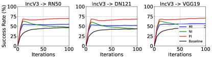
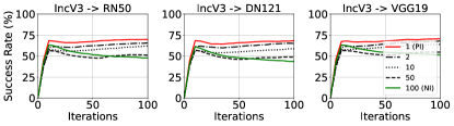
Figure 3: Results for gradient stabilization attacks. Top: Transferability vs. iteration curve. Bottom: Impact of the number of looking-ahead iterations.

4.1 Analysis of Gradient Stabilization Attacks

Figure 3 Top shows the transferability of the three gradient stabilization attacks under various iterations. As can be seen, all three attacks converge very fast, within 10 iterations, since they accumulate gradients with the momentum. However, using more iterations does not necessarily improve but may even harm the performance. This new finding indicates that in practice, we should early stop such attacks in order to ensure optimal transferability. However, it was previously overlooked since existing studies evaluate attacks under only a few iterations, e.g., 10 [14, 38, 74].

Since the above “performance decreasing” phenomenon is newly found, we further explore whether it also applies to the more challenging, targeted attacks. We find that although the results of MI and NI are always lower than 3%, they still require “early stopping” to secure an optimal performance. In contrast, PI indeed does not require “early stopping” and its targeted transferability finally reaches 9.4% on average. This difference between PI for non-targeted and targeted transferability might be because targeted transferability especially requires an accurate direction [101], and PI achieves this through additional looking ahead [74].

When comparing different attacks, we can observe that PI and NI perform better than MI due to looking ahead, but NI is better only at the beginning. The only difference between PI and NI is the maximum number of previous iterations used to look ahead. To figure out the impact of the number of look-ahead iterations, we repeat the experiments with values from 1 (i.e., PI) to 100 (i.e., NI). Figure 3 Bottom shows that the performance drops more as more previous iterations are incorporated to look ahead, and the optimal performance is actually achieved by PI.

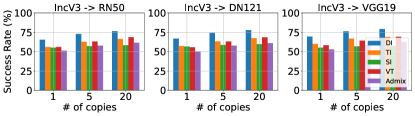
Figure 4: Results for input augmentation attacks. Top: Transferability vs. iteration curve. All attacks use five input copies. Bottom: Impact of the number of input copies.

4.2 Analysis of Input Augmentation Attacks

Figure 4 Top shows the transferability of the five input augmentation attacks under various iterations. Previous evaluations of input augmentation attacks often conduct unfair comparisons where different attacks may leverage a different number of random input copies [73]. Here, in contrast, we compare all attacks under the same number of random input copies. We find that, surprisingly, the earliest attack method, DI, always performs the best, and another early one, TI, performs the second best. However, the latest method, Admix, achieves very low transferability.

We explain the above new finding by comparing the input diversity caused by different attacks since higher input diversity is commonly believed to yield higher transferability [86, 41]. Specifically, we quantify the input diversity of the five attacks by the change of the logit value of the top-1 model prediction caused by their specific augmentations. We calculate the input diversity over 5000 images with 10 repeated runs. We get 0.23 for DI, 0.0017 for TI, 0.00039 for SI, 0.000091 for VT, and -0.035 for Admix. The highest input diversity of DI explains its highest transferability and the lowest input diversity of Admix explains its lowest transferability. In particular, Admix even decreases the original logit value, denoting that it is not a suitable choice for the required label-preserving augmentation.

We further explore the impact of the number of random input copies. Figure 4 Bottom shows that the transferability of all attacks is improved when more copies are used. Specifically, DI and TI consistently perform the best in all settings. This finding suggests the global superiority of spatial transformations (i.e., resizing&padding in DI and translation in TI) over other types of image transformations, such as pixel scaling in SI, additive noise in VT, and image composition in Admix. Note that more copies generally consume more computational resources.

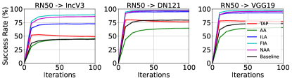
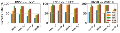
Figure 5: Results for feature disruption attacks. Top: Transferability vs. iteration curve. TAP uses all layers and the others use “conv3_x”. Bottom: Impact of the layers.

4.3 Analysis of Feature Disruption Attacks

Figure 5 Top shows the transferability of the five feature disruption attacks under various iterations. We see that FIA and NAA, which exploit feature importance, achieve the best results. In addition, ILA and TAP perform well, by incorporating the CE loss into their feature-level optimizations. Finally, AA performs even worse than the PGD baseline since it only uses a plain feature loss but ignores the CE loss.

Since all these attacks, except TAP, only disrupt features in a specific layer, we explore the impact of layer choice. As can be seen from Figure 5 Bottom, the last layer (“conv5_x”) performs much worse than the early layers. This might come from the last layer being too complex and model-specific, which results in poor generalizability to unseen models. Moreover, the mid layer (“conv3_x”) always achieves the best performance since it can learn more semantic features than earlier layers, which are known to capture low-level visual attributes, e.g., colors and textures [92].

4.4 Analysis of Surrogate Refinement Attacks

Figure 6 shows the transferability of the five surrogate refinement attacks under various iterations. Here ResNet50 is used as the surrogate model for a fair comparison since SGM [81] can only be applied to architectures with skip connections. We see that IAA achieves the best results mainly because it does not simply integrate specific components (i.e., skip connections and continuous activation functions) but optimizes their hyperparameters towards high transferability. In addition, RFA achieves much lower performance (sometimes even lower than the baseline attack) since it solely uses a robust surrogate model, which is known to have different representation characteristics from the (target) standard model [24, 59, 58].

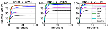
Figure 6: Results for surrogate refinement attacks (1/2): Transferability vs. iteration curve.

Table 6: Results for surrogate refinement attacks (2/2): Impact of the surrogate property. DenseNet121 is used as the target model.

Attacks	Transfer$\uparrow$	Acc$\uparrow$	AI$\uparrow$	AD$\downarrow$	KL$\downarrow$
Original	79.6	100.0	37.4	8.4	14.8
SGM

Model refinement opens a direct way to explore the impact of specific properties of the surrogate model on transferability. Thus we look into model properties in terms of two common metrics: accuracy and interpretability, as well as another specific measure, i.e., model similarity between the surrogate and the target models. Specifically, interpretability is measured by Average Increase (AI) and Average Drop (AD) [8] based on GradCAM [60], and their detailed definitions can be found in Section D. For model similarity, we calculate the Kullback-Leibler (KL) divergence of output features following [25]:

$$KL\mathrel{:=}D_{KL}(softmax(f_{s}(\mathbf{x})[c])||softmax(f_{t}(\mathbf{x})[c])),$$ (8)

where $D_{KL}$ is KL divergence, $f_{s}(\cdot)$ is the surrogate model and $f_{t}(\cdot)$ is the target model. $f(\mathbf{x})[c]$ outputs the logits of the class $c$ given the input $\mathbf{x}$. For LinBP and SGM, we refine the surrogate model not only during backpropagation as in their original implementations but also during the forward pass. This makes sure that the refinement can also potentially influence the model properties besides transferability.

As can be seen from Table 4.4, there is a clear negative correlation between transferability and other model properties. In particular, IAA ranks the highest in terms of transferability but the lowest in terms of all the other four measures of model properties. This is aligned with the previous finding in transfer learning that a pre-trained model that performs well in the target domain does not necessarily perform well in the source domain [58]. In addition, the refinement in LinBP and SGM has little impact on all model properties. This indicates that modifying only the activation function or the hyperparameters of the residual block does not influence the model properties. Specifically, the GradCAM calculations in AI and AD only involve the gradients with respect to the last layer and the ReLU function is applied by default. In addition, for KL, since both the surrogate model and the target model achieve an accuracy of 100%, the above modifications yield small changes in the logit values for the (true) prediction.

Figure 7: Results for generative modeling attacks. Top: Transferability vs. perturbation budget curve. Bottom: Impact of the training perturbation bound, for GAP attack.

4.5 Analysis of Generative Modeling Attacks

As discussed above, generative modeling attacks can be used to generate perturbations under various constraints by simply specifying the corresponding norm bound in the clipping operation. Figure 7 Top shows the transferability of the five generative modeling attacks under various perturbation bounds. For the targeted attack TTP, we calculate its untargeted transferability over 5000 targeted adversarial images that are generated following the 10-Targets setting [47].

As can be seen, the transferability generally increases as the perturbation constraint is relaxed. Consistent with our discussion about feature disruption attacks, feature-level losses (i.e., GAPF and BIA) outperform output-level losses (i.e., GAP and CDA). More specifically, GAPF outperforms BIA probably because GAPF leverages the original, multi-channel feature maps but BIA compresses the feature maps by cross-channel pooling. CDA outperforms GAP since the Relative CE loss in CDA is known to be better than the CE loss in GAP [48]. However, although TTP also adopts a feature-level loss, it falls far behind GAPF and BIA, especially for a small perturbation size. This might be because TTP, as a targeted attack, relies on embedding semantic features (of the target) in the perturbations, which are shown to be difficult when the perturbations are constrained to be small [47, 101].

In addition to the generation/testing stage, the clipping operation is also applied when training the generator. Existing work commonly adopts the perturbation bound $\epsilon_{\textrm{train}}=10$ without exploring the impact of this training perturbation bound on the transferability. To fill this gap, we train the GAP generator with various $\epsilon_{\textrm{train}}$ and test these generators across different perturbation bounds $\epsilon_{\textrm{test}}$. Figure 7 Bottom shows that in general, adjusting $\epsilon_{\textrm{train}}$ has a substantial impact on the transferability. For example, when the $\epsilon_{\textrm{test}}$ is set to 16, varying the $\epsilon_{\textrm{train}}$ from 4 to 32 yields a difference in transferability by about 25%. In addition, using a moderate $\epsilon_{\textrm{train}}$ (i.e. 8-16) consistently leads to the best results for all possible $\epsilon_{\textrm{test}}$. This suggests that it indeed makes sense to set $\epsilon_{\textrm{train}}=10$ as in existing work. However, this finding is somewhat unexpected since choosing the same parameter for model training and testing (here, $\epsilon_{\textrm{train}}=\epsilon_{\textrm{test}}$) normally yields the optimal results in machine learning.

Table 7: Attack transferability in terms of success rate (%). ResNet-50 is used as the surrogate.

Attacks

Without Defenses

Input Pre-processing

Purification Network

Adversarial Training

DN121

VGG19

IncV3

ViT

BDR

PD

R&P

HGD

NRP

DiffPure

AT∞

FD∞

AT2

Clean Acc

5 Comprehensive Evaluation

The intra-category analyses in the above section have provided empirical support for hyperparameter selection in our following large-scale evaluation on attack transferability and stealthiness. Specifically, for gradient stabilization attacks, we set the iteration number to 10 to avoid the “performance decreasing” phenomenon, while for the other three categories of iterative attacks, we set the iteration number to 50 to ensure attack convergence. For input augmentation attacks, we set the number of copies to 5 for a good trade-off between attack strength and efficiency. For feature disruption attacks, we use the mid layer (“conv3_x”), which always yields the best performance. For generative modeling attacks, we set $\epsilon_{\textrm{train}}=10$, which is commonly adopted in existing work and validated to be optimal by our intra-category analyses.

We make sure our findings are stable by repeating our experiments 5 times on 1000 images, each of which is selected from each of the 1000 ImageNet classes. The results confirm that 16 attacks always yield identical numbers because they are deterministic by design. For the other 7 attacks, i.e., the 5 input augmentation attacks, AA, and FIA, the standard deviations are always very small, i.e., standard deviations within [0.001, 0.013] for attack success rates within [0.464, 0.993]. Note that in contrast, there is no statistical analysis in any original work of our considered 23 attacks.

5.1 New Insights into Transferability

Table 4.5 summarizes the transferability results in both the standard and defense settings. These results either lead to new findings or complement existing findings that have been only validated in a limited set of attacks and defenses.

General conclusion: The transferability of an attack against a defense is highly contextual. An attack/defense that performs the best against one specific defense/attack may perform very badly against another. For example, the transferability of CDA to 9 different defenses varies largely, from 3.9% to 100.0%. Similarly, a defense that achieves the highest robustness to one specific attack may be very vulnerable to another attack. For example, the robustness of NRP to 24 different attacks varies largely, from 2.0% to 93.3%.

In particular, we reveal that this contextual performance is related to the overfitting of a defense to the type of perturbations used in its optimization. Specifically, the purification network-based and adversarial training-based defenses rely on training defensive models with additional adversarial data. In this way, the resulting defensive model only ensures high robustness against the perturbations that have been used for generating the adversarial data. We take NRP vs. DiffPure as an example to explain this finding. Specifically, NRP is trained with semantic perturbations [46] and so it is very effective in mitigating low-frequency, semantic perturbations, e.g., those generated by generative modeling attacks (see perturbation visualizations in Figure 8). However, it performs much worse against high-frequency perturbations, e.g., those generated by gradient stabilization and input augmentation attacks. In contrast, DiffPure relies on the diffusion process with (high-frequency) Gaussian noise. Therefore, it is not capable of purifying low-frequency, semantic perturbations. Figure 9 shows that NRP can purify the CDA adversarial images but DiffPure cannot do it well.

The substantial vulnerability of DiffPure to black-box (transferable) attacks is indeed very surprising since DiffPure was initially claimed to provide state-of-the-art robustness to white-box (adaptive) attacks, even surpassing adversarial training [51]. Our finding suggests that DiffPure provides a false sense of security and requires a rightful evaluation following recommendations from [2, 6, 70]. In addition, adversarial training is not effective against RFA since RFA has learned how to distort robust features by adopting an adversarially trained surrogate model. Note that the norm bound used in RFA is $2\times$ larger than that in AT_∞ and FD_∞.

PGD	MI	NI	PI	DI	TI	SI	VT	Admix	TAP	AA	ILA
FIA	NAA	SGM	LinBP	RFA	IAA	DSM	GAP	CDA	GAPF	BIA	TTP

Figure 8: Visualizations of adversarial examples generated by the 24 different attacks with their corresponding perturbations. Additional examples can be found in Appendix E.

Original

CDA

CDA+NRP

CDA+DiffPure

Figure 9: Purifying CDA adversarial images. NRP works well but DiffPure does not due to the defense overfitting problem.

Specific observations:

• Adversarial training is effective but input pre-processing is not. Both the two $L_{\infty}$ adversarial training defenses, AT_∞ and FD_∞, are consistently effective against all attacks except RFA_∞, which uses an adversarially-trained surrogate model for generating robust perturbations. The performance of AT₂ is also not sensitive to the attack method but sub-optimal due to the use of a different, $L_{2}$ norm. In contrast, input pre-processing defenses are generally not useful, although they are known to be effective against (non-adaptive) white-box attacks where the perturbations are much smaller [87, 84].

• Changing the model architecture may be more useful than applying a defense. Previous work has noticed that transferring to Inception-v3 is especially hard [25, 26, 101]. This might be due to the fact that the Inception architecture contains relatively complex components, e.g., multiple-size convolution and two auxiliary classifiers. Our results extend this finding from $\leq 3$ to 23 attacks. Furthermore, transferring from CNNs to ViT is also known to be hard [78, 75, 96]. Based on our results, we can observe that adopting ViT as the target model ranks about 4th on average among the 9 defenses. The above findings suggest that changing the model architecture may be a feasible choice especially when applying a defense consumes more resources.

• New model design largely boosts transferability. The generative modeling attacks and some of the surrogate refinement attacks are based on designing new surrogate or generative models, while the other attacks adopt off-the-shelf surrogate models. In almost all cases, the former attacks outperform the latter. However, they inevitably consume additional computational and data resources.

5.2 New Insights into Stealthiness

Here we compare different attacks on their imperceptibility and also other finer-grained stealthiness characteristics. General conclusion: Stealthiness may be at odds with transferability. Figure 8 visualizes the adversarial images with their corresponding perturbations for different attacks. Solely looking at these examples, we notice that different attacks yield dramatically different perturbations, although they are constrained by the same $L_{\infty}$ norm bound with $\epsilon=16$. In the following, we will demonstrate in more detail the distinct stealthiness characteristics of different attacks.

Imperceptibility. Table 5.2 reports the imperceptibility results for different attacks regarding five diverse perceptual similarity metrics. First of all, almost all the 23 transferable attacks are more perceptible than the PGD baseline although their perturbations are constrained in the same way. This means that the current transferable attacks indeed sacrifice imperceptibility for improving transferability. This finding also suggests that in order to achieve truly imperceptible attacks, using only the $L_{\infty}$ norm during the generation of the perturbations is insufficient. Instead, it requires a comprehensive constraint based on considering diverse perceptual measures. One exception is RFA_∞, which achieves better SSIM performance than the PGD baseline. This might be because RFA_∞ mainly introduces smooth perturbations but does not break image structures too much, as confirmed by the perturbation visualizations in Figure 8.

Moreover, among the 23 transferable attacks, imperceptibility varies greatly and negatively correlates with the transferability reported in Table 4.5. In particular, certain generative modeling attack is the most transferable but also the most perceptible. In addition, generative modeling attacks yield especially large FID scores. This suggests the dramatic distribution shift between their adversarial and original images. This property can be explained by the fact that their adversarial images are image-agnostic, i.e., different images share similar perturbations, as shown in Figure 18 of Appendix E.

Table 8: Imperceptibility regarding five metrics.

Attacks	PSNR$\uparrow$	SSIM$\uparrow$	$\Delta E$$\downarrow$	LPIPS$\downarrow$	FID$\downarrow$
PGD

The above results have demonstrated that different attacks indeed yield dramatically different imperceptibility performance. In the following, we further look into their differences in stealthiness at finer-grained levels. To this end, we conduct “attack traceback”, which aims to trace back the specific attack based on certain information. In general, an attack is less stealthy when it is easier to trace back. The “attack traceback” is basically a classification problem, and in our case, with 24 classes. Specifically, we randomly select 500 original images and then perturb them using the 24 different attacks, resulting in 12000 adversarial images in total. For each attack, 400 adversarial images are used for training and the rest 100 for testing. we conduct the attack classification based on two types of features: (input) image features and (output) misclassification features.

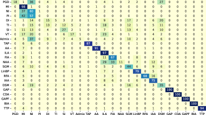
Figure 10: Attack traceback based on image features.

Attack traceback based on image features. We use ResNet-18 as the backbone for the 24-class classifier based on image features. As can be seen from Figure 10, different attacks can be well differentiated solely based on image features, with an overall accuracy of 60.43%, much higher than a random guess, i.e., 1/24. Moreover, the category-wise accuracy is even higher, i.e., 75.61%. This suggests that our new attack categorization is quite reliable since it captures the signature of each specific category.

More specifically, we note low accuracy for PI and input augmentation attacks but perfect accuracy for generative modeling attacks. For PI, the low accuracy might be explained by the similarity between their perturbations and those of NI/MI (see Figure 15 in Appendix E). Similarly, for generative modeling attacks, the perfect accuracy might be explained by their very distinct perturbations. For input augmentation attacks, the perturbations are somewhat a mixture of low- and high-frequency components. So they are harder to distinguish from multiple other attacks. In general, it should be noted that perturbation patterns are hard to categorize, compared to objects that are semantically meaningful to humans.

Table 9: Attack traceback based on misclassification features.

$N$	1	3	5	10	100	1000
Acc (%)	14.6	17.9	18.5	18.1	17.4	17.0

Attack traceback based on misclassification features. We train an SVM classifier with an RBF kernel and adopt the top-$N$ output class IDs as the misclassification features. Table 9 shows the classification accuracy as a function of $N$. As can be seen, too small $N$ is insufficient to represent the attack and too large $N$ may introduce noisy information. In particular, a moderate choice of $N=5$ yields the optimal accuracy, i.e., 18.5%, which is also much higher than a random guess, i.e., 1/24. However, it is still far behind the image features, which have much higher dimensions, i.e., $224\times 224=50176$.

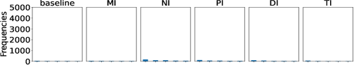
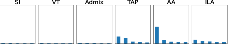
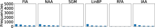
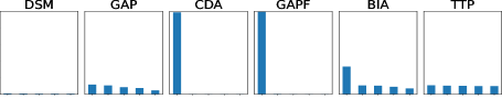
Figure 11: Distributions of five most frequently predicted classes for different attacks.

Figure 12: Distributions of five most frequently predicted classes with their names for one attack in each attack category. Complete results can be found in Appendix E.

We further examine the detailed class distributions of the output predictions. To this end, for each attack, we calculate the frequencies of different classes as the (mis-)prediction over 5000 adversarial images. As can be seen from Figure 11, different attack categories lead to different patterns in their predictions. Specifically, gradient stabilization and input augmentation attacks lead to relatively uniform class distributions, with no specific high-frequent class. In contrast, the other three categories of attacks yield more concentrated distributions. Figure 12 further shows the class names for each attack. We can see that the most frequent class is usually related to semantics that reflects textural patterns, e.g., “brain coral” and “jigsaw puzzle”. This somewhat confirms the high-frequency nature of most perturbations. In addition, the prediction of generative modeling attacks is dominated by specific classes. For example, CDA even fools the model into predicting almost all adversarial images as “harp”. The above findings suggest that generative modeling attacks are very easy to trace back based on misclassification features, even with only the Top-1 prediction.

6 Discussion

6.1 Forward Compatibility

Our attack categorization corresponds to the major components in the common attack pipeline, as shown in Figure 1. Therefore, we believe that future attacks would also fall into those categories unless there appears a completely new design of adversarial attacks. Our evaluation methodology can also be directly extended to other threat models. In the current stage, we have followed the most common threat model as described in Section 3.1. This threat model covers very basic settings regarding models, datasets, constraints, attack goals, etc. In this way, our scientific conclusions would not be affected by specific practical considerations. Exploring more realistic threat models would make more sense with the progress of transferable attacks. For example, targeted attacks pose more realistic threats than non-targeted attacks but most of the current transferable attacks cannot achieve substantial targeted success [101, 47].

6.2 Limitation and Future Work

Our work aims to provide a systematic evaluation of transferable attacks. Although several new conclusions have been drawn, some still need further exploration to be fully understood. For example, we find that for generative modeling attacks, using a moderate $\epsilon_{\textrm{train}}$ leads to consistently optimal performance for all $\epsilon_{\textrm{test}}$, although in normal machine learning, choosing a matched hyperparameter (here $\epsilon_{\textrm{test}}=\epsilon_{\textrm{train}}$) performs the best. This uncommon phenomenon may be specifically related to generative perturbations and requires further study in the future. In addition, we have found that different attacks have dramatically different properties in terms of perturbation and misclassification patterns. Moving forward, it is important to figure out how these properties are related to the specific attack design. In particular, the reason why generative modeling attacks tend to produce image-agnostic perturbations falling into a dominant class should be identified.

7 Conclusion

In this paper, we have provided the first systematic evaluation of recent transferable attacks, involving 23 representative transferable attacks against 9 representative defenses on ImageNet. In particular, we have established new evaluation guidelines that address the two common problems in existing work. Our evaluation focuses on both attack transferability and stealthiness, and our experimental results lead to new insights that complement or even challenge existing knowledge. In particular, for stealthiness, we move beyond diverse imperceptibility measures and explore the potential of attack traceback based on image or misclassification features. Overall, our work aims to give a thorough picture of the current progress of transferable attacks, and we hope that it can guide future research towards good practices in transferable attacks.

Appendix A Descriptions of Attacks and Defenses

A.1 Descriptions of Attacks

Momentum Iterative (MI) [14] integrates the momentum term into the iterative optimization of attacks, in order to stabilize the update directions and escape from poor local maxima. This momentum term accumulates a velocity vector in the gradient direction of the loss function across iterations.

Nesterov Iterative (NI) [38] is based on an improved momentum method that further also leverages the look ahead property of Nesterov Accelerated Gradient (NAG) by making a jump in the direction of previously accumulated gradients before computing the gradients in the current iteration. This makes the attack escape from poor local maxima more easily and faster.

Pre-gradient guided Iterative (PI) [74] follows a similar idea as NI, but it makes a jump based on only the gradients from the last iteration instead of all previously accumulated gradients.

Diverse Inputs (DI) [86] applies random image resizing and padding to the input image before calculating the gradients in each iteration of the attack optimization. This approach aims to prevent attack overfitting (to the white-box, source model), inspired by the data augmentation techniques used for preventing model overfitting.

Translation Invariant (TI) [15] applies random image translations for input augmentation. It also introduces an approximate solution to improve the attack efficiency by directly computing locally smoothed gradients on the original image through the convolution operations rather than computing gradients multiple times for all potential translated images.

Scale Invariant (SI) [38] applies random image scaling for input augmentation. It scales pixels with a factor of $1/2^{i}$. In particular, in each iteration, it takes an average of gradients on multiple augmented images rather than using only one augmented image as in previous input augmentation attacks.

Variance Tuning (VT) [72] applies uniformly distributed additive noise to images for input augmentation and also calculates average gradients over multiple augmented images in each iteration.

Adversarial mixup (Admix) [73] calculates the gradients on a composite image that is made up of the original image and another image randomly selected from an incorrect class. The original image label is still used in the loss function.

Transferable Adversarial Perturbations (TAP) [104] proposes to maximize the distance between original images and their adversarial examples in the intermediate feature space and also introduces a regularization term for reducing the variations of the perturbations and another regularization term with the cross-entropy loss.

Activation Attack (AA) [27] drives the feature-space representation of the original image towards the representation of a target image that is selected from another class. Specifically, AA can achieve targeted misclassification by selecting a target image from that specific target class.

Intermediate Level Attack (ILA) [23] optimizes the adversarial examples in two stages, with the cross-entropy loss used in the first stage to determine the initial perturbations, which will be further fine-tuned in the second stage towards larger feature distance while maintaining the initial perturbation directions.

Feature Importance-aware Attack (FIA) [76] proposes to only disrupts important features. Specifically, it measures the importance of features based on the aggregated gradients with respect to feature maps computed on a batch of transformed original images that are achieved by random image masking.

Neuron Attribution-based Attacks (NAA) [97] relies on an advanced neuron attribution method to measure the feature importance more accurately. It also introduces an approximation approach to conducting neuron attribution with largely reduced computations.

Skip Gradient Method (SGM) [81] suggests using ResNet-like architectures as the source model during creating the adversarial examples. Specifically, it shows that backpropagating gradients through skip connections lead to higher transferability than through the residual modules.

Linear BackPropagation (LinBP) [20] is proposed based on the new finding that the non-linearity of the commonly-used ReLU activation function substantially limits the transferability. To address this limitation, the ReLU is replaced by a linear function during only the backpropagation process.

Robust Feature-guided Attack (RFA) [65] proposes to use an adversarially-trained model (with $L_{2}$ or $L_{\infty}$ bound) as the source model based on the assumption that modifying more robust features yields more generalizable (transferable) adversarial examples.

Intrinsic Adversarial Attack (IAA) [105] finds that disturbing the intrinsic data distribution is the key to generating transferable adversarial examples. Based on this, it optimizes the hyperparameters of the Softplus and the weights of skip connections per layer towards aligned attack directions and data distribution.

Dark Surrogate Model (DSM) [88] is trained from scratch with additional “dark” knowledge, which is achieved by training with soft labels from a pre-trained teacher model and using data augmentation techniques, such as Cutout, Mixup, and CutMix.

Generative Adversarial Perturbations (GAP) [55] proposes a new attack approach that is based on generative modeling. Specifically, it uses the source classifier as the discriminator and trains a generator using the cross-entropy loss. Once trained, the generator can be used to generate an adversarial example for each input original image with only one forward pass.

Cross-Domain Attack (CDA) [48] follows the GAP pipeline but uses a more advanced loss (i.e., relativistic cross entropy) to train the generator. This new loss explicitly enforces the probability gap between the clean and adversarial images, boosting the transferability, especially in cross-domain scenarios.

Transferable Targeted Perturbations (TTP) [47] is focused on improving transferability of targeted attacks. It is based on learning target-specific generators, each of which is trained with the objective of matching the distribution of targeted perturbations with that of data from a specific target class. Specifically, input augmentation and smooth perturbation projection are used to further boost the performance.

Generative Adversarial Feature Perturbations (GAFP) [29] follows the general pipeline of GAP but trains the generator using a loss that maximizes the feature map distance between adversarial and original images at mid-level CNN layers.

Beyond ImageNet Attack (BIA) [98] also follows the general pipeline of GAP and specifically introduces a random normalization module to simulate different training data distributions and also a feature distance loss that is only based on important/generalizable features.

A.2 Descriptions of Defenses

Bit-Depth Reduction (BDR) [87] pre-processes input images by reducing the color depth of each pixel while maintaining the semantics. This operation can eliminate pixel-level adversarial perturbations from adversarial images but has little impact on model predictions of clean images.

Pixel Deflection (PD) [56] pre-processes input images by randomly replacing some pixels with randomly selected pixels from their local neighborhood. It is specifically designed to happen more frequently to non-salient pixels, and a subsequent wavelet-based denoising operation is used to soften the corruption.

Resizing and Padding (R&P) [84] pre-processes input images by random resizing, which resizes the input images to a random size, and then random padding, which pads zeros around the resized input images.

High-level representation Guided Denoiser (HGD) [37] learns a purification network that can be used to purify/denoise the adversarial perturbations. Specifically, different from previous methods that focus on image-space denoising, HGD minimizes the difference between the clean image and the denoised image at intermediate feature layers.

Neural Representation Purifier (NRP) [46] learns a purification network using a combined loss that calculates both the image- and feature-space differences. Specifically, the adversarial images used for training the purification network are generated by feature loss-based adversaries, which are shown to be more effective in handling unseen attacks.

Diffusion Purification (DiffPure) [51] uses a diffusion model as the purification network. It diffuses an input image by gradually adding noise in a forward diffusion process and then recovers the clean image by gradually denoising the image in a reverse generative process. The reverse process is shown to be also capable of removing adversarial perturbations.

$L_{\infty}$-Adversarial Training (AT_∞) [85] follows the basic pipeline of adversarial training, which is to train the robust model on adversarial images. Specifically, these adversarial images are generated using the PGD targeted attacks with the $L_{\infty}$ distance, and the model is trained distributedly on 128 Nvidia V100 GPUs.

$L_{\infty}$-Adversarial Training with Feature Denoising (FD_∞) [85] modifies the standard model architecture by introducing new building blocks that are designed for denoising feature maps based on non-local means or other filters. This modification can help suppress the potential disruptions caused by the adversarial perturbations, and the modified model is trained end-to-end.

$L_{2}$-Adversarial Training (AT₂) [58] trains the model on adversarial images that are generated using the PGD non-targeted attacks with the $L_{2}$ distance.

A.3 Hyperparameters of Attacks and Defenses

Table 10: Hyperparameters of attacks and defenses.

Attacks	Hyperparameter
MI [14]	decay factor $\mu=1$
NI [38]	decay factor $\mu=1$
PI [74]	decay factor $\mu=1$
DI [86]	resize&pad range $R=[1,~{}1.1]$ transformation probability $p=0.7$
TI [15]	translation range $R=[-2,2]$
SI [38]	scale range $R=[0.1,1]$
VT [72]	noise range $R=[-1.5\epsilon,1.5\epsilon]$
Admix [73]	mixing factor $\eta=0.2$
TAP [104]	$\lambda=0.005$, $\eta=0.01$, $\alpha=0.5$
AA [27]	$20$ random target images from 4 classes
ILA [23]	ILA projection loss
FIA [76]	$N=30$, $P_{\mathrm{drop}}=0.3$
NAA [97]	$N=30$, $\gamma=1.0$, linear transformation
SGM [81]	decay parameter $\gamma=0.5$
LinBP [20]	first residual unit in the third meta block
RFA [65]	$L_{2}$ $\epsilon=0.1$ or $L_{\infty}$ $\epsilon=8$ PGD-AT
IAA [105]	$\beta=15$
DSM [88]	CutMix augmentation
GAP [55]	ResNet152 discriminator
CDA [48]	ResNet152 discriminator
GAPF [29]	ResNet152 discriminator
BIA [98]	ResNet152 discriminator, RN module
TTP [47]	ResNet50 discriminator
Defenses	Hyperparameters
BDR [87]	bit depth $D=2$
PD [56]	R-CAM: $k=5$, denoising: $\sigma=0.04$
R&P [84]	resize&pad range $R=[1,~{}1.1]$
HGD [37]	ResNet152-Wide
NRP [46]	ResNet (1.2M parameters)
DiffPure [51]	noise level $t=150$ WideResNet-50-2
AT∞ [85]	$L_{\infty}$ $\epsilon=8$, PGD iters $n=30$, lr=$\alpha=1$
FD∞ [85]	$L_{\infty}$ $\epsilon=8$, PGD iters $n=30$, lr=$\alpha=1$
AT2 [58]	$L_{2}$ $\epsilon=3.0$, PGD iters $n=7$, lr=$\alpha=0.5$

Appendix B Existing Evaluations

Table 11: Evaluation comparisons in existing studies. ( ) means fully (partially) following the “New vs. Old” manner.

Studies	# of attacks (categories)	New vs. Old
MI [14]	1 (1)
NI [38]	4 (2)
PI [74]	5 (2)
DI [86]	2 (2)
TI [15]	3 (2)
SI [38]	4 (2)
VT [72]	6 (2)
Admix [73]	4 (1)
TAP [104]	2 (2)
AA [27]	2 (2)
ILA [23]	4 (3)
FIA [76]	6 (3)
NAA [97]	5 (2)
SGM [81]	4 (3)
LinBP [20]	5 (3)
RFA [65]	1 (1)
IAA [105]	7 (4)
DSM [88]	4 (3)
GAP [55]	1 (1)
CDA [48]	9 (4)
GAPF [29]	3 (1)
BIA [98]	5 (3)
TTP [47]	11 (5)
Ours	23 (5)

Appendix C Imperceptibility Metrics

Peak Signal-to-Noise Ratio (PSNR) measures the ratio of the maximum possible power of a signal (image $\mathbf{x}$) to the noise (perturbations $\mathbf{\sigma}$) power. It is calculated by:

$$\textrm{PSNR}(\mathbf{x},\mathbf{\sigma})=10\cdot\log_{10}\frac{\max(\mathbf{x})^{2}}{\textrm{MSE}(\mathbf{x},\mathbf{\sigma})},$$ (9)

where the Mean Squared Error (MSE) measures the average squared difference between the two inputs.

Structural Similarity Index Measure (SSIM) [77] is used for measuring the perceptual quality of digital images. In our case, it measures the structural similarity between the original image $\mathbf{x}$ and adversarial image $\mathbf{x}^{\prime}$, which is considered to be a degraded version of $\mathbf{x}$. It is calculated by:

$$\textrm{SSIM}(\mathbf{x},\mathbf{x}^{\prime})=\frac{{(2\mu_{\mathbf{x}}\mu_{\mathbf{x}^{\prime}}+c_{1})+(2\sigma_{\mathbf{x}\mathbf{x}^{\prime}}+c_{2})}}{(\mu_{\mathbf{x}}^{2}+\mu_{\mathbf{x}^{\prime}}^{2}+c_{1})(\sigma_{\mathbf{x}}^{2}+\sigma_{\mathbf{x}^{\prime}}^{2}+c_{2})}.$$ (10)

Descriptions of $c_{1}$ and $c_{1}$ and more technical details can be found in [77].

$\Delta$E [43] refers to the CIE $\Delta E$ standard formula used for measuring the perceptual color distance between two pixels. We follow [100] to use the latest variant, CIEDE2000, since it is shown to align very well with human perception. It is calculated in the CIELCH space by:

$$\begin{gathered}\Delta E=\sqrt{(\frac{\Delta L^{\prime}}{k_{L}S_{L}})^{2}+(\frac{\Delta C^{\prime}}{k_{C}S_{C}})^{2}+(\frac{\Delta H^{\prime}}{k_{H}S_{H}})^{2}+\Delta R},\\ \Delta R=R_{T}(\frac{\Delta C^{\prime}}{k_{C}S_{C}})(\frac{\Delta H^{\prime}}{k_{H}S_{H}}),\end{gathered}$$ (11)

where $\Delta L^{\prime}$, $\Delta C^{\prime}$, $\Delta H^{\prime}$ denotes the distance between two pixels in their lightness, chroma, and hue channels, respectively. $\Delta R$ is an interactive term between chroma and hue differences. Detailed definitions and explanations of the weighting functions ($S_{L}$, $S_{C}$, $S_{H}$ and $R_{T}$) and hyperparameters $k_{L}$, $k_{C}$ and $k_{H}$ can be found in [43]. Further, Image-level perceptual color difference is obtained by computing the $L_{2}$ norm of the above $\Delta E$ for each pixel.

Learned Perceptual Image Patch Similarity (LPIPS) [99] is developed for measuring the perceptual similarity between two images. It computes the cosine distance (in the channel dimension) between features at each given convolutional layer $l$ and averages the results across spatial dimensions $H\times W$ and layers of a specific network $f$:

$$\textrm{LPIPS}=\sum_{l}\frac{1}{H_{l}W_{l}}\sum_{h,w}\cos(f^{l}_{hw}(\mathbf{x}),f^{l}_{hw}(\mathbf{x}^{\prime})),$$ (12)

where AlexNet is adopted as $f$ for computational efficiency.

Frechet Inception Distance (FID) [67] is originally used to assess the quality of generated images and can also be used to assess the quality of adversarial images. It compares the distribution of adversarial images to that of original images. Specifically, the output features from the pool3 layer of an Inception-V3 for original and adversarial images are used to fit two multidimensional Gaussian distributions $\mathcal{N}(\mu,\Sigma)$ and $\mathcal{N}(\mu^{\prime},\Sigma^{\prime})$, and the FID score is calculated by:

$$\textrm{FID}(\mathcal{N}(\mu,\Sigma),\mathcal{N}(\mu^{\prime},\Sigma^{\prime}))=\|\mu\textendash\mu^{\prime}\|_{2}^{2}+\textrm{tr}(\Sigma+\Sigma^{\prime}-2\sqrt{\Sigma\Sigma^{\prime}}),$$ (13)

where tr denotes the trace of the matrix.

Appendix D Interpretability Metrics

For model interpretability, we adopt two metrics, Average Increase (AI) and Average Drop (AD), from [8]. Let $p^{c}_{i}$ and $o^{c}_{i}$ be the predicted probability for the ground-truth class $c$ given as input the $i$-th image $\mathbf{x}_{i}$ and its masked version, and let $n$ be the number of test images. AI measures the percentage of images where the masked image yields a higher class probability than the original (higher is better):

$$\operatorname{AI}~{}(\%)\mathrel{:=}\frac{1}{n}\sum_{i}^{n}\mathbb{1}_{p^{c}_{i}<o^{c}_{i}}\cdot 100$$ (14)

AD quantifies how much predictive power, measured as class probability, is lost when only the masked regions of the image are used (lower is better):

$$\operatorname{AD}~{}(\%)\mathrel{:=}\frac{1}{n}\sum_{i=1}^{n}\frac{[p^{c}_{i}-o^{c}_{i}]_{+}}{p^{c}_{i}}\cdot 100.$$ (15)

Appendix E Additional Visulizations

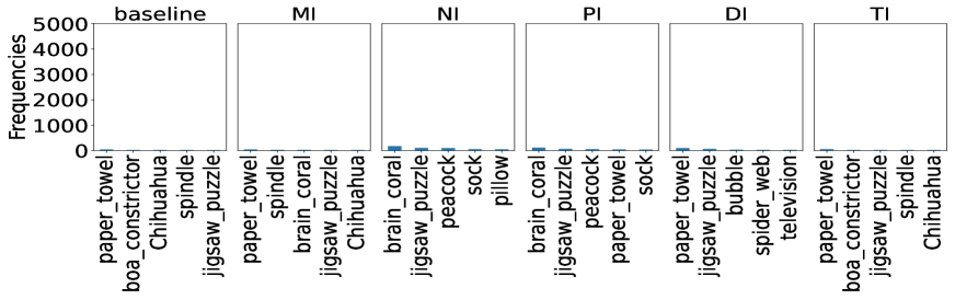
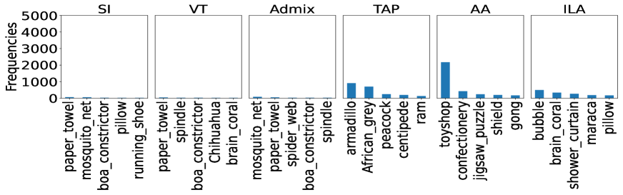
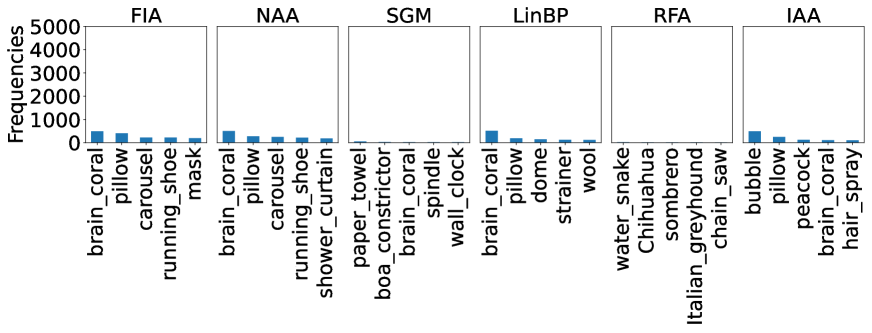
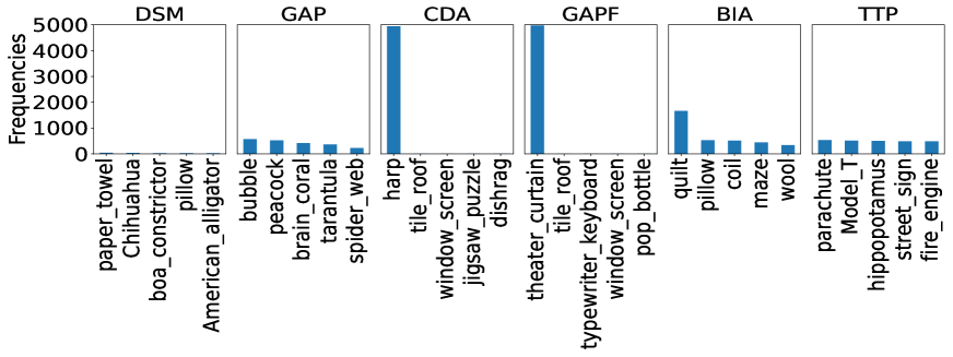
Figure 13: Distributions of five most frequently predicted classes with their names.

Original
PGD
MI
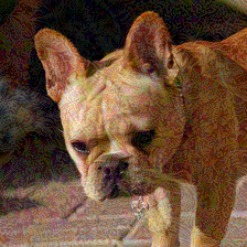
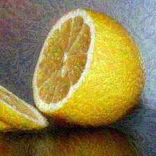
NI
PI

Figure 14: Adversarial examples generated by gradient stabilization attacks and the PGD baseline, along with original images.

DI
TI
SI
VT
Admix

Figure 15: Adversarial examples generated by input augmentation attacks.

TAP
AA
ILA
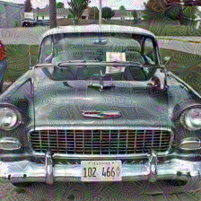
FIA
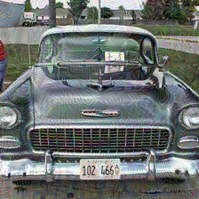
NAA

Figure 16: Adversarial examples generated by feature disruption attacks.

SGM
LinBP
RFA
IAA
DSM

Figure 17: Adversarial examples generated by surrogate refinement attacks.

GAP
CDA
GAPF
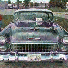
BIA
TTP

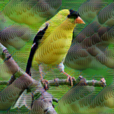
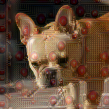
Figure 18: Adversarial examples generated by generative modeling attacks.

References

- [1] Rima Alaifari, Giovanni S Alberti, and Tandri Gauksson. ADef: an iterative algorithm to construct adversarial deformations. In ICLR, 2019.
- [2] Anish Athalye, Nicholas Carlini, and David Wagner. Obfuscated gradients give a false sense of security: Circumventing defenses to adversarial examples. In ICML, 2018.
- [3] Anand Bhattad, Min Jin Chong, Kaizhao Liang, Bo Li, and David A Forsyth. Unrestricted adversarial examples via semantic manipulation. In ICLR, 2020.
- [4] Battista Biggio and Fabio Roli. Wild patterns: Ten years after the rise of adversarial machine learning. Pattern Recognition, 84:317–331, 2018.
- [5] Junyoung Byun, Seungju Cho, Myung-Joon Kwon, Hee-Seon Kim, and Changick Kim. Improving the transferability of targeted adversarial examples through object-based diverse input. In CVPR, 2022.
- [6] Nicholas Carlini, Anish Athalye, Nicolas Papernot, Wieland Brendel, Jonas Rauber, Dimitris Tsipras, Ian Goodfellow, Aleksander Madry, and Alexey Kurakin. On evaluating adversarial robustness. In arXiv, 2019.
- [7] Nicholas Carlini and David Wagner. Towards evaluating the robustness of neural networks. In IEEE S&P, 2017.
- [8] A. Chattopadhay, A. Sarkar, P. Howlader, and V. N. Balasubramanian. Grad-CAM++: Generalized gradient-based visual explanations for deep convolutional networks. In WACV, 2018.
- [9] Sizhe Chen, Qinghua Tao, Zhixing Ye, and Xiaolin Huang. Measuring attacks by the norm. In ICASSP, 2023.
- [10] Steven Chen, Nicholas Carlini, and David Wagner. Stateful detection of black-box adversarial attacks. In SPAI, 2020.
- [11] Francesco Croce and Matthias Hein. Sparse and imperceivable adversarial attacks. In ICCV, 2019.
- [12] Edoardo Debenedetti, Nicholas Carlini, and Florian Tramèr. Evading black-box classifiers without breaking eggs. In ICML Workshop on Frontiers in AdvML, 2023.
- [13] Zhun Deng, Linjun Zhang, Kailas Vodrahalli, Kenji Kawaguchi, and James Y Zou. Adversarial training helps transfer learning via better representations. In NeurIPS, 2021.
- [14] Yinpeng Dong, Fangzhou Liao, Tianyu Pang, Hang Su, Jun Zhu, Xiaolin Hu, and Jianguo Li. Boosting adversarial attacks with momentum. In CVPR, 2018.
- [15] Yinpeng Dong, Tianyu Pang, Hang Su, and Jun Zhu. Evading defenses to transferable adversarial examples by translation-invariant attacks. In CVPR, 2019.
- [16] Alexey Dosovitskiy, Lucas Beyer, Alexander Kolesnikov, Dirk Weissenborn, Xiaohua Zhai, Thomas Unterthiner, Mostafa Dehghani, Matthias Minderer, Georg Heigold, Sylvain Gelly, et al. An image is worth 16x16 words: Transformers for image recognition at scale. In ICLR, 2021.
- [17] Aditya Ganeshan, Vivek BS, and R Venkatesh Babu. FDA: Feature disruptive attack. In ICCV, 2019.
- [18] Ian Goodfellow, Jean Pouget-Abadie, Mehdi Mirza, Bing Xu, David Warde-Farley, Sherjil Ozair, Aaron Courville, and Yoshua Bengio. Generative adversarial nets. In NeurIPS, 2014.
- [19] Ian Goodfellow, Jonathon Shlens, and Christian Szegedy. Explaining and harnessing adversarial examples. In ICLR, 2015.
- [20] Yiwen Guo, Qizhang Li, and Hao Chen. Backpropagating linearly improves transferability of adversarial examples. In NeurIPS, 2020.
- [21] Kaiming He, Xiangyu Zhang, Shaoqing Ren, and Jian Sun. Deep residual learning for image recognition. In CVPR, 2016.
- [22] Gao Huang, Zhuang Liu, Laurens Van Der Maaten, and Kilian Q Weinberger. Densely connected convolutional networks. In CVPR, 2017.
- [23] Qian Huang, Isay Katsman, Horace He, Zeqi Gu, Serge Belongie, and Ser-Nam Lim. Enhancing adversarial example transferability with an intermediate level attack. In ICCV, 2019.
- [24] Andrew Ilyas, Shibani Santurkar, Dimitris Tsipras, Logan Engstrom, Brandon Tran, and Aleksander Madry. Adversarial examples are not bugs, they are features. In NeurIPS, 2019.
- [25] Nathan Inkawhich, Kevin Liang, Lawrence Carin, and Yiran Chen. Transferable perturbations of deep feature distributions. In ICLR, 2020.
- [26] Nathan Inkawhich, Kevin J Liang, Binghui Wang, Matthew Inkawhich, Lawrence Carin, and Yiran Chen. Perturbing across the feature hierarchy to improve standard and strict blackbox attack transferability. In NeurIPS, 2020.
- [27] Nathan Inkawhich, Wei Wen, Hai Helen Li, and Yiran Chen. Feature space perturbations yield more transferable adversarial examples. In CVPR, 2019.
- [28] Can Kanbak, Seyed-Mohsen Moosavi-Dezfooli, and Pascal Frossard. Geometric robustness of deep networks: analysis and improvement. In CVPR, 2018.
- [29] Krishna kanth Nakka and Mathieu Salzmann. Learning transferable adversarial perturbations. In NeurIPS, 2021.
- [30] Simon Kornblith, Mohammad Norouzi, Honglak Lee, and Geoffrey Hinton. Similarity of neural network representations revisited. In ICML, 2019.
- [31] Alexey Kurakin, Ian Goodfellow, and Samy Bengio. Adversarial examples in the physical world. In ICLR, 2017.
- [32] Maosen Li, Cheng Deng, Tengjiao Li, Junchi Yan, Xinbo Gao, and Heng Huang. Towards transferable targeted attack. In CVPR, 2020.
- [33] Qizhang Li, Yiwen Guo, and Hao Chen. Yet another intermediate-level attack. In ECCV, 2020.
- [34] Yingwei Li, Song Bai, Cihang Xie, Zhenyu Liao, Xiaohui Shen, and Alan L Yuille. Regional homogeneity: Towards learning transferable universal adversarial perturbations against defenses. In ECCV, 2020.
- [35] Yingwei Li, Song Bai, Yuyin Zhou, Cihang Xie, Zhishuai Zhang, and Alan L Yuille. Learning transferable adversarial examples via ghost networks. In AAAI, 2020.
- [36] Kaizhao Liang, Jacky Y Zhang, Boxin Wang, Zhuolin Yang, Sanmi Koyejo, and Bo Li. Uncovering the connections between adversarial transferability and knowledge transferability. In ICML, 2021.
- [37] Fangzhou Liao, Ming Liang, Yinpeng Dong, Tianyu Pang, Xiaolin Hu, and Jun Zhu. Defense against adversarial attacks using high-level representation guided denoiser. In CVPR, 2018.
- [38] Jiadong Lin, Chuanbiao Song, Kun He, Liwei Wang, and John E Hopcroft. Nesterov accelerated gradient and scale invariance for adversarial attacks. In ICLR, 2020.
- [39] Yanpei Liu, Xinyun Chen, Chang Liu, and Dawn Song. Delving into transferable adversarial examples and black-box attacks. In ICLR, 2017.
- [40] Zhuoran Liu, Zhengyu Zhao, and Martha Larson. Who’s afraid of adversarial queries? the impact of image modifications on content-based image retrieval. In ICMR, 2019.
- [41] Yuyang Long, Qilong Zhang, Boheng Zeng, Lianli Gao, Xianglong Liu, Jian Zhang, and Jingkuan Song. Frequency domain model augmentation for adversarial attack. In ECCV, 2022.
- [42] Bo Luo, Yannan Liu, Lingxiao Wei, and Qiang Xu. Towards imperceptible and robust adversarial example attacks against neural networks. In AAAI, 2018.
- [43] Ming Ronnier Luo, Guihua Cui, and B. Rigg. The development of the CIE 2000 colour-difference formula: CIEDE2000. Color Research and Application, 26:340–350, 2001.
- [44] Aleksander Madry, Aleksandar Makelov, Ludwig Schmidt, Dimitris Tsipras, and Adrian Vladu. Towards deep learning models resistant to adversarial attacks. In ICLR, 2018.
- [45] Yuhao Mao, Chong Fu, Saizhuo Wang, Shouling Ji, Xuhong Zhang, Zhenguang Liu, Jun Zhou, Alex X Liu, Raheem Beyah, and Ting Wang. Transfer attacks revisited: A large-scale empirical study in real computer vision settings. In SP, 2022.
- [46] Muzammal Naseer, Salman Khan, Munawar Hayat, Fahad Shahbaz Khan, and Fatih Porikli. A self-supervised approach for adversarial robustness. In CVPR, 2020.
- [47] Muzammal Naseer, Salman Khan, Munawar Hayat, Fahad Shahbaz Khan, and Fatih Porikli. On generating transferable targeted perturbations. In ICCV, 2021.
- [48] Muzammal Naseer, Salman H Khan, Harris Khan, Fahad Shahbaz Khan, and Fatih Porikli. Cross-domain transferability of adversarial perturbations. In NeurIPS, 2019.
- [49] Muzammal Naseer, Salman H Khan, Shafin Rahman, and Fatih Porikli. Task-generalizable adversarial attack based on perceptual metric. In arXiv, 2018.
- [50] Yurii Evgen’evich Nesterov. A method of solving a convex programming problem with convergence rate obigl(k^2bigr). In Doklady Akademii Nauk, 1983.
- [51] Weili Nie, Brandon Guo, Yujia Huang, Chaowei Xiao, Arash Vahdat, and Anima Anandkumar. Diffusion models for adversarial purification. In ICML, 2022.
- [52] Nicolas Papernot, Patrick McDaniel, Ian Goodfellow, Somesh Jha, Z Berkay Celik, and Ananthram Swami. Practical black-box attacks against machine learning. In AsiaCCS, 2017.
- [53] Nicolas Papernot, Patrick McDaniel, Somesh Jha, Matt Fredrikson, Z Berkay Celik, and Ananthram Swami. The limitations of deep learning in adversarial settings. In EuroS&P, 2016.
- [54] Boris T Polyak. Some methods of speeding up the convergence of iteration methods. Ussr computational mathematics and mathematical physics, 1964.
- [55] Omid Poursaeed, Isay Katsman, Bicheng Gao, and Serge Belongie. Generative adversarial perturbations. In CVPR, 2018.
- [56] Aaditya Prakash, Nick Moran, Solomon Garber, Antonella DiLillo, and James Storer. Deflecting adversarial attacks with pixel deflection. In CVPR, 2018.
- [57] Andras Rozsa, Ethan M Rudd, and Terrance E Boult. Adversarial diversity and hard positive generation. In CVPRW, 2016.
- [58] Hadi Salman, Andrew Ilyas, Logan Engstrom, Ashish Kapoor, and Aleksander Madry. Do adversarially robust imagenet models transfer better? In NeurIPS, 2020.
- [59] Shibani Santurkar, Dimitris Tsipras, Brandon Tran, Andrew Ilyas, Logan Engstrom, and Aleksander Madry. Computer vision with a single (robust) classifier. In NeurIPS, 2019.
- [60] Ramprasaath R Selvaraju, Michael Cogswell, Abhishek Das, Ramakrishna Vedantam, Devi Parikh, and Dhruv Batra. Grad-cam: Visual explanations from deep networks via gradient-based localization. In ICCV, 2017.
- [61] Ali Shahin Shamsabadi, Ricardo Sanchez-Matilla, and Andrea Cavallaro. ColorFool: Semantic adversarial colorization. In CVPR, 2020.
- [62] Mahmood Sharif, Lujo Bauer, and Michael K. Reiter. On the suitability of -norms for creating and preventing adversarial examples. In CVPRW, 2018.
- [63] Karen Simonyan and Andrew Zisserman. Very deep convolutional networks for large-scale image recognition. In ICLR, 2015.
- [64] Gowthami Somepalli, Liam Fowl, Arpit Bansal, Ping Yeh-Chiang, Yehuda Dar, Richard Baraniuk, Micah Goldblum, and Tom Goldstein. Can neural nets learn the same model twice? investigating reproducibility and double descent from the decision boundary perspective. In CVPR, 2022.
- [65] Jacob M Springer, Melanie Mitchell, and Garrett T Kenyon. A little robustness goes a long way: Leveraging robust features for targeted transfer attacks. In NeurIPS, 2021.
- [66] Mukund Sundararajan, Ankur Taly, and Qiqi Yan. Axiomatic attribution for deep networks. In ICML, 2017.
- [67] Christian Szegedy, Vincent Vanhoucke, Sergey Ioffe, Jon Shlens, and Zbigniew Wojna. Rethinking the inception architecture for computer vision. In CVPR, 2016.
- [68] Christian Szegedy, Wojciech Zaremba, Ilya Sutskever, Joan Bruna, Dumitru Erhan, Ian Goodfellow, and Rob Fergus. Intriguing properties of neural networks. In ICLR, 2014.
- [69] Florian Tramèr, Jens Behrmann, Nicholas Carlini, Nicolas Papernot, and Jörn-Henrik Jacobsen. Fundamental tradeoffs between invariance and sensitivity to adversarial perturbations. In ICML, 2020.
- [70] Florian Tramer, Nicholas Carlini, Wieland Brendel, and Aleksander Madry. On adaptive attacks to adversarial example defenses. In NeurIPS, 2020.
- [71] Francisco Utrera, Evan Kravitz, N Benjamin Erichson, Rajiv Khanna, and Michael W Mahoney. Adversarially-trained deep nets transfer better: Illustration on image classification. In ICLR, 2021.
- [72] Xiaosen Wang and Kun He. Enhancing the transferability of adversarial attacks through variance tuning. In CVPR, 2021.
- [73] Xiaosen Wang, Xuanran He, Jingdong Wang, and Kun He. Admix: Enhancing the transferability of adversarial attacks. In ICCV, 2021.
- [74] Xiaosen Wang, Jiadong Lin, Han Hu, Jingdong Wang, and Kun He. Boosting adversarial transferability through enhanced momentum. In BMVC, 2021.
- [75] Yuxuan Wang, Jiakai Wang, Zixin Yin, Ruihao Gong, Jingyi Wang, Aishan Liu, and Xianglong Liu. Generating transferable adversarial examples against vision transformers. In ACMMM, 2022.
- [76] Zhibo Wang, Hengchang Guo, Zhifei Zhang, Wenxin Liu, Zhan Qin, and Kui Ren. Feature importance-aware transferable adversarial attacks. In ICCV, 2021.
- [77] Zhou Wang, Alan C. Bovik, Hamid R. Sheikh, and Eero P. Simoncelli. Image quality assessment: from error visibility to structural similarity. IEEE Transactions On Image Processing, 13:600–612, 2004.
- [78] Zhipeng Wei, Jingjing Chen, Micah Goldblum, Zuxuan Wu, Tom Goldstein, and Yu-Gang Jiang. Towards transferable adversarial attacks on vision transformers. In AAAI, 2022.
- [79] Zhipeng Wei, Jingjing Chen, Zuxuan Wu, and Yu-Gang Jiang. Incorporating locality of images to generate targeted transferable adversarial examples. In arXiv, 2022.
- [80] Eric Wong, Frank Schmidt, and Zico Kolter. Wasserstein adversarial examples via projected sinkhorn iterations. In ICML, 2019.
- [81] Dongxian Wu, Yisen Wang, Shu-Tao Xia, James Bailey, and Xingjun Ma. Skip connections matter: On the transferability of adversarial examples generated with ResNets. In ICLR, 2020.
- [82] Weibin Wu, Yuxin Su, Xixian Chen, Shenglin Zhao, Irwin King, Michael R Lyu, and Yu-Wing Tai. Boosting the transferability of adversarial samples via attention. In CVPR, 2020.
- [83] Chaowei Xiao, Jun-Yan Zhu, Bo Li, Warren He, Mingyan Liu, and Dawn Song. Spatially transformed adversarial examples. In ICLR, 2018.
- [84] Cihang Xie, Jianyu Wang, Zhishuai Zhang, Zhou Ren, and Alan Yuille. Mitigating adversarial effects through randomization. In ICLR, 2018.
- [85] Cihang Xie, Yuxin Wu, Laurens van der Maaten, Alan L Yuille, and Kaiming He. Feature denoising for improving adversarial robustness. In CVPR, 2019.
- [86] Cihang Xie, Zhishuai Zhang, Yuyin Zhou, Song Bai, Jianyu Wang, Zhou Ren, and Alan L Yuille. Improving transferability of adversarial examples with input diversity. In CVPR, 2019.
- [87] Weilin Xu, David Evans, and Yanjun Qi. Feature squeezing: Detecting adversarial examples in deep neural networks. In NDSS, 2018.
- [88] Dingcheng Yang, Zihao Xiao, and Wenjian Yu. Boosting the adversarial transferability of surrogate model with dark knowledge. In ICTAI, 2023.
- [89] Xiao Yang, Yinpeng Dong, Tianyu Pang, Hang Su, and Jun Zhu. Boosting transferability of targeted adversarial examples via hierarchical generative networks. In ECCV, 2022.
- [90] Jason Yosinski, Jeff Clune, Yoshua Bengio, and Hod Lipson. How transferable are features in deep neural networks? In NeurIPS, 2014.
- [91] Zheng Yuan, Jie Zhang, and Shiguang Shan. Adaptive image transformations for transfer-based adversarial attack. In ECCV, 2022.
- [92] Matthew D Zeiler and Rob Fergus. Visualizing and understanding convolutional networks. In ECCV, 2014.
- [93] Chaoning Zhang, Philipp Benz, Gyusang Cho, Adil Karjauv, Soomin Ham, Chan-Hyun Youn, and In So Kweon. Backpropagating smoothly improves transferability of adversarial examples. In CVPR Workshop on AML, 2021.
- [94] Chaoning Zhang, Gyusang Cho, Philipp Benz, Kang Zhang, Chenshuang Zhang, Chan-Hyun Youn, and In So Kweon. Early stop and adversarial training yield better surrogate model: Very non-robust features harm adversarial transferability. In OpenReview, 2021.
- [95] Hanwei Zhang, Yannis Avrithis, Teddy Furon, and Laurent Amsaleg. Smooth adversarial examples. EURASIP Journal on Information Security, 2020.
- [96] Jianping Zhang, Yizhan Huang, Weibin Wu, and Michael R Lyu. Transferable adversarial attacks on vision transformers with token gradient regularization. In CVPR, 2023.
- [97] Jianping Zhang, Weibin Wu, Jen-tse Huang, Yizhan Huang, Wenxuan Wang, Yuxin Su, and Michael R Lyu. Improving adversarial transferability via neuron attribution-based attacks. In CVPR, 2022.
- [98] Qilong Zhang, Xiaodan Li, Yuefeng Chen, Jingkuan Song, Lianli Gao, Yuan He, and Hui Xue. Beyond imagenet attack: Towards crafting adversarial examples for black-box domains. In ICLR, 2022.
- [99] Richard Zhang, Phillip Isola, Alexei A Efros, Eli Shechtman, and Oliver Wang. The unreasonable effectiveness of deep features as a perceptual metric. In CVPR, 2018.
- [100] Zhengyu Zhao, Zhuoran Liu, and Martha Larson. Towards large yet imperceptible adversarial image perturbations with perceptual color distance. In CVPR, 2020.
- [101] Zhengyu Zhao, Zhuoran Liu, and Martha Larson. On success and simplicity: A second look at transferable targeted attacks. In NeurIPS, 2021.
- [102] Zhengyu Zhao, Zhuoran Liu, and Martha Larson. Adversarial image color transformations in explicit color filter space. IEEE Transactions on Information Forensics and Security, 2023.
- [103] Bolei Zhou, Aditya Khosla, Agata Lapedriza, Aude Oliva, and Antonio Torralba. Learning deep features for discriminative localization. In CVPR, 2016.
- [104] Wen Zhou, Xin Hou, Yongjun Chen, Mengyun Tang, Xiangqi Huang, Xiang Gan, and Yong Yang. Transferable adversarial perturbations. In ECCV, 2018.
- [105] Yao Zhu, Jiacheng Sun, and Zhenguo Li. Rethinking adversarial transferability from a data distribution perspective. In ICLR, 2022.
- [106] Junhua Zou, Zhisong Pan, Junyang Qiu, Xin Liu, Ting Rui, and Wei Li. Improving the transferability of adversarial examples with resized-diverse-inputs, diversity-ensemble and region fitting. In ECCV, 2020.