High-Order Methods

Our starting point is given by the conservation law

$$\frac{\partial U}{\partial t}+\nabla\cdot\mathbf{F}=0\qquad\rightarrow\qquad\int\frac{\partial U}{\partial t}\,d^{3}x=-\oint\mathbf{F}\cdot\,d\mathbf{S}$$ (1)

which becomes

$$\frac{d\left<\mathbf{U}\right>}{dt}=-\frac{\Delta t}{\Delta V}\oint\mathbf{F}\cdot d\mathbf{S}=-\frac{\Delta t}{\Delta V}\sum_{d}\left<F\right>_{d}S_{d}$$ (2)

where $d=i\pm\frac{1}{2},j\pm\frac{1}{2},k\pm\frac{1}{2}$ spans across faces.

1 Flux Equivalence between 2D and 3D ?

We want to check the conditions under which a 3D problem with a cyclic coordinate ($z$) is n in a equivalent way to a 2D problem. We start by considering the Godunov flux of $B_{z}$ at an $x$-interface computed in 2D:

$$\left.F^{[B_{z}]}\right|_{i+\frac{1}{2}}=\left.E_{y}\right|_{i+\frac{1}{2}}=\frac{F^{[B_{z}]}_{L}+F^{[B_{z}]}_{R}}{2}-\frac{|\lambda_{x}|}{2}\left(B_{z,R}-B_{z,L}\right)$$ (3)

Where $L,R$ refer to the $i+\frac{1}{2}$ interface. Since $F^{[B_{z}]}=B_{z}v_{x}-B_{x}v_{z}$, we have

$$\left.F^{[B_{z}]}\right|_{i+\frac{1}{2}}=\left.E_{y}\right|_{i+\frac{1}{2}}=\frac{(B_{z}v_{x}-B_{x}v_{z})_{L}+(B_{z}v_{x}-B_{x}v_{z})_{R}}{2}-\frac{|\lambda_{x}|}{2}\left(B_{z,R}-B_{z,L}\right)$$ (4)

Since $B_{x}$ is unique at an $x$-interface,

$$\boxed{\left.F^{[B_{z}]}\right|_{i+\frac{1}{2}}=\left.E_{y}\right|_{i+\frac{1}{2}}=\frac{(B_{z}v_{x})_{L}+(B_{z}v_{x})_{R}-B_{x,i+\frac{1}{2}}(v_{z,L}+v_{z,R})}{2}-\frac{|\lambda_{x}|}{2}\left(B_{z,R}-B_{z,L}\right)}$$ (5)

In the 3D case, the emf is obtained by interpolating contributions from the $i+\frac{1}{2}$ interface and the $k+\frac{1}{2}$ interface:

$$\boxed{\begin{array}[]{lcl}\displaystyle\left.E_{y}\right|_{i+\frac{1}{2},k+\frac{1}{2}}&=&\displaystyle-\frac{(B_{x}v_{z})_{S}+(B_{x}v_{z})_{N}}{2}+\frac{(B_{z}v_{x})_{W}+(B_{z}v_{x})_{E}}{2}\\ \vskip 6.0pt plus 2.0pt minus 2.0pt\cr&&\displaystyle-\frac{|\lambda_{x}|}{2}\left(B_{z,E}-B_{z,W}\right)+\frac{|\lambda_{z}|}{2}\left(B_{x,N}-B_{x,S}\right)\end{array}}$$ (6)

where $S,N$ indicate reconstructions in the $z$-direction from the $i+\frac{1}{2}$ interfaces (with $k$ and $k+1$) while $W,E$ indicate reconstructions in the $x$-direction from $k+\frac{1}{2}$ interfaces (with $i$ and $i+1$):

$$(v_{z})_{S}={\cal R}^{z}_{+}\left(\frac{v_{z,i+\frac{1}{2},L}+v_{z,i+\frac{1}{2},R}}{2}\right)\quad\underline{or}\quad(v_{z})_{S}=\frac{1}{2}\left[{\cal R}^{z}_{+}\left(v_{z,i+\frac{1}{2},L}\right)+{\cal R}^{z}_{+}\left(v_{z,I+\frac{1}{2},R}\right)\right]$$ (7)

$$(v_{x})_{W}={\cal R}^{x}_{+}\left(\frac{v_{x,k+\frac{1}{2},L}+v_{x,k+\frac{1}{2},R}}{2}\right)\quad\underline{or}\quad(v_{z})_{W}=\frac{1}{2}\left[{\cal R}^{x}_{+}\left(v_{x,k+\frac{1}{2},L}\right)+{\cal R}^{x}_{+}\left(v_{x,k+\frac{1}{2},R}\right)\right]$$ (8)

Although formally equivalent, the two choices in Eq. (7) and Eq. (8) may produce differences in the full 3D case. In PLUTO, the first choice is employed since only one reconstruction is performed. For a graphical representation of the various symbols, have a look at Fig. 1.

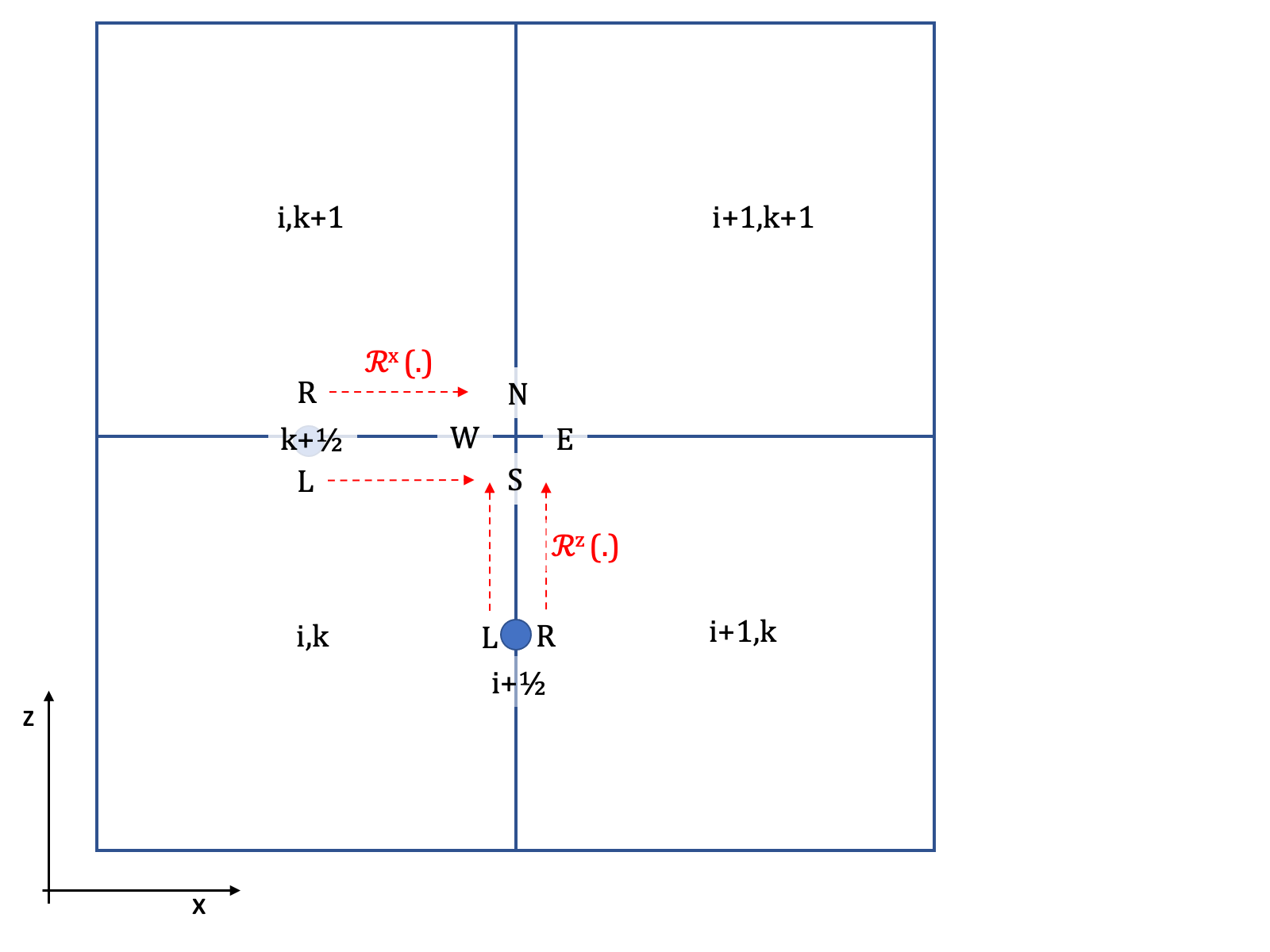
Figure 1: Grid quantities representation. The $y$-direction is redundant since no interpolation is ever carried in the y-direction when computing $E_{y}$.

Is Eq. (6) equivalent to Eq. (5) when the $z$ coordinate is ignorable ?
In this case $\partial_{z}=0$, $B_{x,N}=B_{x,S}$ and Eq. (7) becomes

$$(v_{z})_{S}=(v_{z})_{N}=\frac{v_{z,L}+v_{z,R}}{2}$$ (9)

where we have used the fact that ${\cal R}^{z}(q)=q$ when $\partial_{z}=0$. Likewise, Eq. (7) becomes

$$(v_{x})_{W}=v_{x,i+\frac{1}{2},L}\,,\quad(v_{x})_{E}=v_{x,i+\frac{1}{2},R}\,,\quad$$ (10)

so that Eq. (6) simplifies to

$$\begin{array}[]{lcl}\displaystyle\left.E_{y}\right|_{i+\frac{1}{2},k+\frac{1}{2}}&=&\displaystyle-\frac{(B_{x}v_{z})_{S}+(B_{x}v_{z})_{N}}{2}+\frac{(B_{z}v_{x})_{W}+(B_{z}v_{x})_{E}}{2}-\frac{|\lambda_{x}|}{2}\left(B_{z,E}-B_{z,W}\right)+\frac{|\lambda_{z}|}{2}\left(B_{x,N}-B_{x,S}\right)\\ \vskip 6.0pt plus 2.0pt minus 2.0pt\cr&=&\displaystyle-B_{x,i+\frac{1}{2}}\frac{v_{z,L}+v_{z,R}}{2}+\frac{(B_{z}v_{x})_{W}+(B_{z}v_{x})_{E}}{2}-\frac{|\lambda_{x}|}{2}\left(B_{z,E}-B_{z,W}\right)\\ \vskip 6.0pt plus 2.0pt minus 2.0pt\cr&=&\displaystyle-B_{x,i+\frac{1}{2}}\frac{v_{z,L}+v_{z,R}}{2}+\frac{(B_{z}v_{x})_{L}+(B_{z}v_{x})_{R}}{2}-\frac{|\lambda_{x}|}{2}\left(B_{z,R}-B_{z,L}\right)\end{array}$$ (11)

which is the same as Eq. (5).

2 Reconstruction from Volumes

1. Using standard polynomial approach inside the $i$-th zone,

   $$q_{i}(x)=a_{0}+a_{1}x+a_{2}x^{2}+\cdots+a_{n}x^{n}$$ (12)

   where $a_{0},\dots,a_{n}$ are coefficients for the polynomial in zone $i$. We now impose $n+1$ conditions, namely that in each cell of the stencil, the line average of the primitive quantitity:

   $$\left<q\right>_{k}=\frac{1}{\Delta x}\int_{x_{k-\frac{1}{2}}}^{x_{k+\frac{1}{2}}}Q(x)\,dx$$

   with $k=i-n/2,i-n/2+1,\dots,i,i+1,\dots,i+n/2$ coincides with the evaluation of the polynomial at the cell center.
   Once the coefficients have been found, since the polynomial is unique, the interface value inside zone $i$ is

   $$q_{i+\frac{1}{2}}^{L}=q_{i}(x+\Delta x/2)$$ (13)

2. Using derivative of the primitive function.
   Consider:

   $$Q(x)=\int^{x}_{-\infty}q(s)\,ds\qquad\Longrightarrow\qquad\frac{dQ}{dx}=q(x)$$ (14)

   Therefore

   $$q_{i+\frac{1}{2}}^{L}=\left.\frac{dQ}{dx}\right|_{i+\frac{1}{2}}$$ (15)

   For a second order approximation, one could use, for instance:

   $$\left.\frac{dQ}{dx}\right|_{i+\frac{1}{2}}=\frac{Q_{i+3/2}-Q_{i-1/2}}{2\Delta x}+O(\Delta x^{2})=\frac{1}{2\Delta x}\left(\int^{x_{i+3/2}}q(s)\,ds-\int^{x_{i-1/2}}q(s)\,ds\right)$$ (16)

   and finally

   $$=\frac{1}{2}\left[\sum_{k=-\infty}^{i+1}\left<q\right>_{k}-\sum_{k=-\infty}^{i-1}\left<q\right>_{k}\right]=\frac{\left<q\right>_{i}+\left<q\right>_{i+1}}{2}$$ (17)

   If we use a fourth-order central difference approximation to evaluate the derivative on the right hand side:

   $$\left.\frac{dQ}{dx}\right|_{i+\frac{1}{2}} =\frac{Q_{i-3/2}-8Q_{i-1/2}+8Q_{i+3/2}-Q_{i+5/2}}{12\Delta x}+O(\Delta x^{4})$$

   $$=\frac{1}{12\Delta x}\left(\int^{x_{i-3/2}}q(s)\,ds-8\int^{x_{i-1/2}}q(s)\,ds+8\int^{x_{i+3/2}}q(s)\,ds-\int^{x_{i+5/2}}q(s)\,ds\right)$$

   $$=\frac{1}{12\Delta x}\left(7\int^{x_{i+1/2}}_{x_{i-1/2}}q(s)\,ds+7\int^{x_{i+3/2}}_{x_{i+1/2}}q(s)\,ds-\int^{x_{i-1/2}}_{x_{i-3/2}}q(s)\,ds-\int^{x_{i+5/2}}_{x_{i+3/2}}q(s)\,ds\right)$$

   $$=\frac{7}{12}\left(\left<q\right>_{i}+\left<q\right>_{i+1}\right)-\frac{1}{12}\left(\left<q\right>_{i-1}+\left<q\right>_{i+2}\right)$$

   For the MP5, the logical procedure is the same, but the approximation to the first derivative is:

   1. Fifth-order accurate;

   2. Non-symmetric wrt the cell-center, but symmetric wrt the $i+\frac{1}{2}$ interface;

   $$\left.\frac{dQ}{dx}\right|_{i+\frac{1}{2}} =\frac{-2Q_{i-5/2}+15Q_{i-3/2}-60Q_{i-1/2}+20Q_{i+1/2}+30Q_{i+3/2}-3Q_{i+5/2}}{60\Delta x}+O(\Delta x^{5})$$

   $$=\frac{1}{60\Delta x}\left($$

   $$\quad+20\int^{x_{i+1/2}}q(s)\,ds+30\int^{x_{i+3/2}}q(s)\,ds-3\int^{x_{i+5/2}}q(s)\,ds\right)$$

   $$=\frac{1}{60\Delta x}\left($$

   $$\quad-3\int^{x_{i+5/2}}_{x_{i+3/2}}q(s)\,ds\right)$$

   $$=\frac{1}{60}\left(2\left<q\right>_{i-2}-13\left<q\right>_{i-1}+47\left<q\right>_{i}+27\left<q\right>_{i+1}-3\left<q\right>_{i+2}\right)$$

   The WENO approach uses a different phylosophy: the $N$ point stencil is splitted into $(N-2)$ sub-stencils of $(N-2)$ points each. Each stencil is used to fit a polynomium of degree $(N-3)$, and the polynomials are then carefully combined in a convex combination obtaining a $N-th$ order accurate interpolating curve.

   In our case we are interested in the WENOZ approach, where $N=5$. The substencils serve to fit 3 parabolas (thus $2^{nd}$-order accuracy), which are then combined to yield a $5^{th}$-order accurate polynomium with some special properties (e.g. monotonicity, non-oscillatory behaviour and so forth).

   $$\left.\ q(x)\right|_{i+\frac{1}{2}}=\omega_{0}\frac{2q_{i-2}-7q_{i-1}+11q_{i}}{6}+\omega_{1}\frac{-q_{i-1}+5q_{i}+2q_{i+1}}{6}+\omega_{2}\frac{2q_{i}+5q_{i+1}-q_{i+2}}{6}$$

   Where the weights $\omega_{0},\omega_{1},\omega_{2}$ represent the weight of each parabola in the final convex combination. The actual definition and properties of these weights will be discussed later, now we are interested in defining the optimal weights.

   With optimal weights we refer to the specific numerical values to substitute in the previous equation to obtain the MP5 rule. These optimal weights have the values of:

   $(\omega_{0}=\frac{1}{10},\omega_{1}=\frac{6}{10},\omega_{2}=\frac{3}{10})$.

   By substituting them in the WENOZ formula, one obtains exactly the MP5 rule.

3 Reconstruction from Point Values

There are many ways to interpolate a polynomial on a set of given punctual values (e.g. solving for the Vandermonde matrix, Lagrange polynomials etc), the most useful for our purposes are:

1. Approach using Taylor expansion:

   $$q_{i+\frac{1}{2}}=q_{i}+q^{\prime}_{i}\frac{\Delta x}{2}+\frac{1}{2!}q^{\prime\prime}_{i}\left(\frac{\Delta x}{2}\right)^{2}$$

   For example, using a 3-point stencil:

   $$q^{\prime}_{i}=\frac{q_{i+1}-q_{i-1}}{2\Delta x}\,,\qquad q^{\prime\prime}_{i}=\frac{q_{i+1}-2q_{i}+q_{i-1}}{\Delta x^{2}}\,,\qquad$$

2. Standard polynomial approach:

   To evaluate the coefficients for the MP5 algorithm using punctual values we consider the quartic curve:

   $$q_{i}(x)=a_{0}+a_{1}x+a_{2}x^{2}+a_{3}x^{3}+a_{4}x^{4}$$ (18)

   and the tuple:

   $$\left\{(x_{i-2},v_{i-2}),(x_{i-1},v_{i-1}),(x_{i},v_{i}),(x_{i+1},v_{i+1}),(x_{i+2},v_{i+2})\right\}$$ (19)

   where $x_{k}$ is the cell center and $v_{k}$ is the punctual value of the function evaluated at $x_{k}$,
   with: $k=i-2\cdots i+2$

   We determine the unique value of the coefficients $a_{0},a_{1},a_{2},a_{3},a_{4}$ by imposing that the polynomial evaluated at $x_{k}$ assumes the value $v_{k}$.
   We thus obtain the following linear system of equations:

   $$\begin{cases}q_{i-2}&=v_{i-2}=a_{0}+a_{1}(x_{i-2})+a_{2}(x_{i-2})^{2}+a_{3}(x_{i-2})^{3}+a_{4}(x_{i-2})^{4}\\ q_{i-1}&=v_{i-1}=a_{0}+a_{1}(x_{i-1})+a_{2}(x_{i-1})^{2}+a_{3}(x_{i-1})^{3}+a_{4}(x_{i-1})^{4}\\ q_{i}&=v_{i}\quad=a_{0}+a_{1}(x_{i})+a_{2}(x_{i})^{2}+a_{3}(x_{i})^{3}+a_{4}(x_{i})^{4}\\ q_{i+1}&=v_{i+1}=a_{0}+a_{1}(x_{i+1})+a_{2}(x_{i+1})^{2}+a_{3}(x_{i+1})^{3}+a_{4}(x_{i+1})^{4}\\ q_{i+2}&=v_{i+2}=a_{0}+a_{1}(x_{i+2})+a_{2}(x_{i+2})^{2}+a_{3}(x_{i+2})^{3}+a_{4}(x_{i+2})^{4}\end{cases}$$

   considering:

   $$\left\{x_{i-2}=-2,x_{i-1}=-1,x_{i}=0,x_{i+1}=+1,x_{i+2}=+2\right\}$$ (20)

   we obtain:

   $$\begin{cases}q_{i-2}&=v_{i-2}=a_{0}-2a_{1}+4a_{2}-8a_{3}+16a_{4}\\ q_{i-1}&=v_{i-1}=a_{0}-a_{1}+a_{2}-a_{3}+a_{4}\\ q_{i}&=v_{i}\quad=a_{0}\\ q_{i+1}&=v_{i+1}=a_{0}+a_{1}+a_{2}+a_{3}+a_{4}\\ q_{i+2}&=v_{i+2}=a_{0}+2a_{1}+4a_{2}+8a_{3}+16a_{4}\end{cases}$$

   By summing and subtracting groups of equations we solve for the parameters:

   $$\begin{cases}a_{0}&=v_{i}\\ a_{1}&=\frac{1}{12}\left(v_{i-2}-8v_{i-1}+8v_{i+1}-v_{i+2}\right)\\ a_{2}&=\frac{1}{24}\left(-v_{i-2}+16v_{i-1}-30v_{i}+16v_{i+1}-v_{i+2}\right)\\ a_{3}&=\frac{1}{12}\left(v_{i+2}-2v_{i+1}+2v_{i-1}-v_{i-2}\right)\\ a_{4}&=\frac{1}{24}\left(v_{i+2}-4v_{i+1}+6v_{i}-4v_{i+1}+v_{i+2}\right)\end{cases}$$

   And thus, by evaluating $\left.\ q(x)\right|_{i+\frac{1}{2}}$ we obtain:

   $$\left\{\frac{45}{64}v_{i},\frac{3}{128}v_{i-2},\frac{-5}{128}v_{i+2},\frac{-5}{32}v_{i-1},\frac{15}{32}v_{i+1}\right\}$$

   Or:

   $$\left.\ q(x)\right|_{i+\frac{1}{2}}=\frac{1}{128}\left(3v_{i-2}-20v_{i-1}+90v_{i}+60v_{i+1}-5v_{i+2}\right)$$

   For the WENOZ reconstruction, at first, we find the expressions of the three parabolas obtained in each sub-stencil by the interpolation using punctual values. The full stencil is constitued by the tuple:

   $$\left\{(x_{i-2},v_{i-2}),(x_{i-1},v_{i-1}),(x_{i},v_{i}),(x_{i+1},v_{i+1}),(x_{i+2},v_{i+2})\right\}$$ (21)

   , while each sub-stencil is given by:

   $$S_{1} =\left\{(x_{i-2},v_{i-2}),(x_{i-1},v_{i-1}),(x_{i},v_{i})\right\}$$

   $$S_{2} =\left\{(x_{i-1},v_{i-1}),(x_{i},v_{i}),(x_{i+1},v_{i+1})\right\}$$

   $$S_{3} =\left\{(x_{i},v_{i}),(x_{i+1},v_{i+1}),(x_{i+2},v_{i+2})\right\}$$

   Polynomial I: On $S_{1}$ we solve for the polynomial $q_{i}(x)=a_{0}+a_{1}x+a_{2}x^{2}$ with $\left\{x_{i-2}=-2,x_{i-1}=-1,x_{i}=0\right\}$. We obtain the system:

   $$\begin{cases}q_{i-2}&=v_{i-2}=a_{0}+a_{1}(x_{i-2})+a_{2}(x_{i-2})^{2}\\ q_{i-1}&=v_{i-1}=a_{0}+a_{1}(x_{i-1})+a_{2}(x_{i-1})^{2}\\ q_{i}&=v_{i}\quad=a_{0}+a_{1}(x_{i})+a_{2}(x_{i})^{2}\\ \end{cases}$$

   which gives:

   $$\begin{cases}q_{i-2}&=v_{i-2}=a_{0}-2a_{1}+4a_{2}\\ q_{i-1}&=v_{i-1}=a_{0}-a_{1}+a_{2}\\ q_{i}&=v_{i}\quad=a_{0}\\ \end{cases}$$

   The solution to the system evaluated at the interface $i+\frac{1}{2}$ is:

   $$P_{L}=\left.\ q(x)\right|_{i+\frac{1}{2}}=\frac{1}{8}\left(3v_{i-2}-10v_{i-1}+15v_{i}\right)$$

   Polynomial II: On $S_{2}$ we solve for the polynomial $q_{i}(x)=a_{0}+a_{1}x+a_{2}x^{2}$ with $\left\{x_{i-1}=-1,x_{i}=0,x_{i+1}=+1\right\}$. We obtain the system:

   $$\begin{cases}q_{i-1}&=v_{i-1}=a_{0}+a_{1}(x_{i-1})+a_{2}(x_{i-1})^{2}\\ q_{i}&=v_{i}\quad=a_{0}+a_{1}(x_{i})+a_{2}(x_{i})^{2}\\ q_{i+1}&=v_{i+1}=a_{0}+a_{1}(x_{i+1})+a_{2}(x_{i+1})^{2}\\ \end{cases}$$

   which gives:

   $$\begin{cases}q_{i-1}&=v_{i-1}=a_{0}-a_{1}+a_{2}\\ q_{i}&=v_{i}\quad=a_{0}\\ q_{i+1}&=v_{i+1}=a_{0}+a_{1}+a_{2}\\ \end{cases}$$

   The solution to the system evaluated at the interface $i+\frac{1}{2}$ is:

   $$P_{C}=\left.\ q(x)\right|_{i+\frac{1}{2}}=\frac{1}{8}\left(-v_{i-i}+6v_{i}+3v_{i+1}\right)$$

   Polynomial III: On $S_{3}$ we solve for the polynomial $q_{i}(x)=a_{0}+a_{1}x+a_{2}x^{2}$ with $\left\{x_{i}=0,x_{i+1}=+1,x_{i+2}=+2\right\}$. We obtain the system:

   $$\begin{cases}q_{i}&=v_{i}\quad=a_{0}+a_{1}(x_{i})+a_{2}(x_{i})^{2}\\ q_{i+1}&=v_{i+1}=a_{0}+a_{1}(x_{i+1})+a_{2}(x_{i+1})^{2}\\ q_{i+2}&=v_{i+2}=a_{0}+a_{1}(x_{i+2})+a_{2}(x_{i+2})^{2}\end{cases}$$

   which gives:

   $$\begin{cases}q_{i}&=v_{i}\quad=a_{0}\\ q_{i+1}&=v_{i+1}=a_{0}+a_{1}+a_{2}\\ q_{i+2}&=v_{i+2}=a_{0}+2a_{1}+4a_{2}\end{cases}$$

   The solution to the system evaluated at the interface $i+\frac{1}{2}$ is:

   $$P_{R}=\left.\ q(x)\right|_{i+\frac{1}{2}}=\frac{1}{8}\left(3v_{i}+6v_{i+1}-v_{i+2}\right)$$

   Now we have to find the optimal convex combination of these parabolas to yield the $5^{th}$-order polynomial which is specified by the MP5 rule. The condition is:

   $$\left.\ q(x)\right|_{i+\frac{1}{2}} =\frac{C_{L}}{8}\left(3v_{i-2}-10v_{i-1}+15v_{i}\right)+\frac{C_{C}}{8}\left(-v_{i-i}+6v_{i}+3v_{i+1}\right)+\frac{C_{R}}{8}\left(3v_{i}+6v_{i+1}-v_{i+2}\right)$$

   $$=\frac{1}{128}\left(3v_{i-2}-20v_{i-1}+90v_{i}+60v_{i+1}-5v_{i+2}\right)$$

   plus a normalization condition $C_{L}+C_{C}+C_{R}=1$.

   Thanks to the Theorem of uniqueness of the interpolating polynomial, we can impose some constraint on this equation: we consider the polynomial $P_{WENOZ}=C_{L}P_{L}+C_{C}P_{C}+C_{R}P_{R}$.

   We take the coefficients of the terms $v_{i}=\frac{3}{4}C_{C}+\frac{15}{8}C_{L}+\frac{3}{8}C_{R},v_{i+1}=\frac{3}{8}C_{C}+\frac{3}{4}C_{R}$ and force it to be equal to the same coefficients obtained with the MP5 method. By considering also the normalization condition we can express one of the coefficients as: $C_{C}=1-C_{L}-C_{R}$ and obtain the following linear system:

   $$\begin{cases}\frac{3}{4}+\frac{9}{8}C_{L}-\frac{3}{8}C_{R}&=\frac{45}{64}\\ \frac{3}{8}-\frac{3}{8}C_{L}+\frac{3}{8}C_{R}&=\frac{15}{32}\end{cases}$$

   By solving this system we obtain the optimal weights to be:

   $$\left\{C_{L}=\frac{1}{16},C_{C}=\frac{5}{8},C_{R}=\frac{5}{16}\right\}$$

3.1 On the benefit of punctual reconstructions on ghost zones

In this section we compare our numerical scheme with the one proposed by Felker and Stone (2018). We both make use of 4 ghost zones for the high-order numerical scheme with the CT scheme for DivB control but at different computational costs.

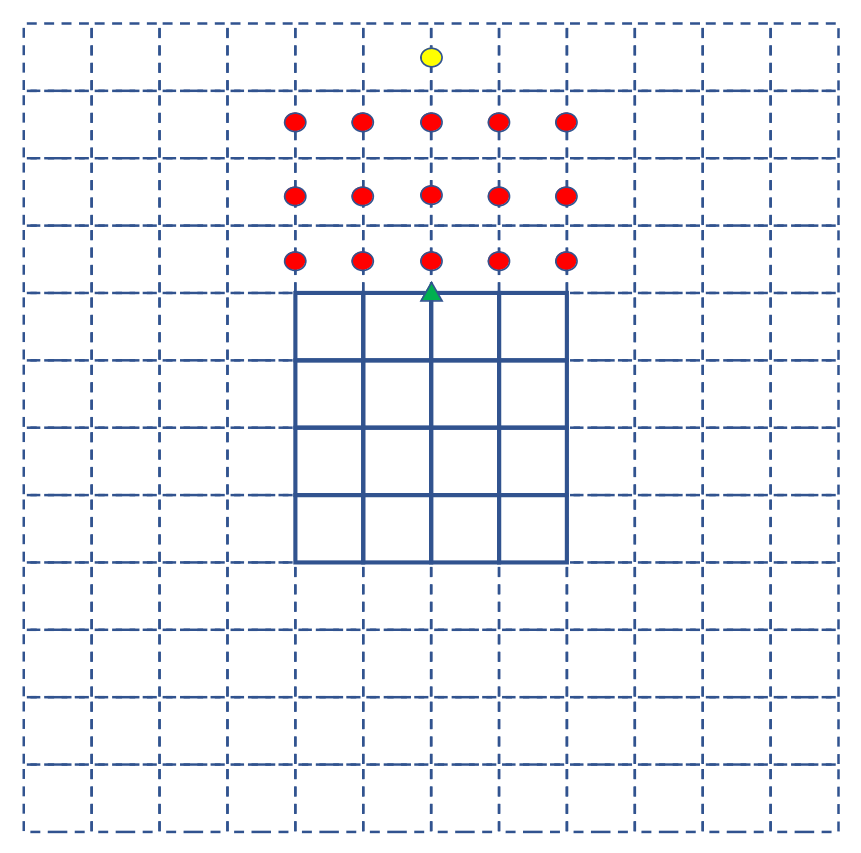
Figure 2: Pictorial representation of the logical structure of the computational domain. The blue lines represent the active domain, dashed blue lines are the ghost zones, red and yellow dots are respectively the high and low-order punctual fluxes needed in the CT scheme, and green triangles are the E field at edges. Our numerical scheme does not require the solution of Riemann problems at yellow dots.

At high order accuracy, 4 ghost zones are needed both longitudinally and transversely for reconstruction operations along the sweep directions. When adopting a CT scheme for DivB control, even 5 ghosts would be required due to reconstruction of the Electric field at edges.

• Felker and Stone (2018): in order to evaluate the high-order E field at edges (green triangle), a reconstruction step using the punctual high-order fluxes (red points) is needed. However, since the reconstructions implemented in this scheme make use of average values, an additional $2^{nd}$-order Riemann problem (yellow dot) is solved to convolve even the bordering points to $4^{th}$-order accuracy. This strategy uses 4 ghost zones, but at the cost of one additional Riemann problem per sweep direction per reconstruction.

• Mignone and Berta (202?) approach: in our numerical scheme we reach the goal of 4 ghost zones without the cost of additional Riemann problems by means of punctual reconstructions. We tested the validity of punctual reconstructions by means of a strict comparison of the log files produced in a set of simulations. We compared the outputs of: 8 vs 5 ghost zones simulations using traditional average-value reconstructions, and 8 vs 4 ghost zones simulations performed via the new punctual reconstruction. The numerical tests executed were the 2D-3D Circularly Polarized Alfvèn waves, the 2D Isentropic vortex, the Orszag-Tang vortex and the MHD Blast wave. Each set of comparisons has been run with different configurations: WENOZ vs MP5 volume vs punctual reconstructions combined with CT vs GLM schemes.

We can conclude that our scheme is more efficient than that proposed by Felker and Stone.

Figure 3: EMF Domain of Dependence in the PLUTO code.

4 Divergence-Free Reconstruction

Statement of the problem: given the face-average of the staggered magnetic field, and (for example) its $1^{\rm st}$ and $2^{\rm nd}$ derivatives at face, find the point-value at the center and its volume average.

We will first face this problem in its 2D version. We first write the polynomials for $B_{x}(x,y)$ and $B_{y}(x,y)$ inside the cell $x,y\in[-\frac{1}{2},\frac{1}{2}]\times[-\frac{1}{2},\frac{1}{2}]$:

$$\begin{array}[]{lcll}B_{x}&=&a_{0}&\to\,{\rm Order}\;0\\ &&\displaystyle+a_{x}x+a_{y}y&\to\,{\rm Order}\;1\\ &&\displaystyle+a_{xx}x^{2}+a_{yy}y^{2}+a_{xy}xy&\to\,{\rm Order}\;2\\ &&\displaystyle+a_{xxx}x^{3}+a_{3y}y^{3}+a_{xxy}x^{2}y+a_{xyy}xy^{2}&\to\,{\rm Order}\;3\\ \vskip 6.0pt plus 2.0pt minus 2.0pt\cr B_{y}&=&c_{0}&\to\,{\rm Order}\;0\\ &&\displaystyle+c_{x}x+c_{y}y&\to\,{\rm Order}\;1\\ &&\displaystyle+c_{xx}x^{2}+c_{yy}y^{2}+c_{xy}xy&\to\,{\rm Order}\;2\\ &&\displaystyle+c_{xxx}x^{3}+c_{yyy}y^{3}+c_{xxy}x^{2}y+c_{xyy}xy^{2}&\to\,{\rm Order}\;3\end{array}$$

In total we have 20 coefficients and therefore 20 unknowns.

The conditions are:

$$\begin{array}[]{l}\displaystyle\left<B_{x}\right>_{\pm\frac{1}{2},0}=\int B_{x}\left(\pm\frac{1}{2},y\right)\,dy\\ \vskip 6.0pt plus 2.0pt minus 2.0pt\cr\displaystyle\left<B_{y}\right>_{0,\pm\frac{1}{2}}=\int B_{y}\left(x,\pm\frac{1}{2}\right)\,dx\\ \vskip 6.0pt plus 2.0pt minus 2.0pt\cr\displaystyle\left.\frac{\partial B_{x}}{\partial y}\right|_{\pm\frac{1}{2},0},\quad\left.\frac{\partial B_{y}}{\partial x}\right|_{0,\pm\frac{1}{2}},\quad\left.\frac{\partial^{2}B_{x}}{\partial y^{2}}\right|_{\pm\frac{1}{2},0},\quad\left.\frac{\partial^{2}B_{y}}{\partial x^{2}}\right|_{0,\pm\frac{1}{2}}\end{array}$$ (22)

The previous relations provides $12$ conditions but only $11$ are independent since the divergence of $\mathbf{B}$ is satisfied at the discrete level giving:

$$\left(\left<B_{x}\right>_{+\frac{1}{2},0}-\left<B_{x}\right>_{-\frac{1}{2},0}\right)+\left(\left<B_{y}\right>_{0,+\frac{1}{2}}-\left<B_{y}\right>_{0,-\frac{1}{2}}\right)=0$$

Thus Eq. (22) gives $11$ independent constraints (= known values) in total. Additional constraints come by imposing the $\nabla\cdot\mathbf{B}=0$ constraint in a continuous sense:

$$\nabla\cdot\mathbf{B}=\frac{\partial B_{x}}{\partial x}+\frac{\partial B_{y}}{\partial y}=\alpha_{0}+\alpha_{x}x+\alpha_{y}y+\alpha_{xy}xy+\alpha_{xx}x^{2}+\alpha_{yy}y^{2}=0$$

which gives $6$ additional constraints: $\alpha_{0}=\alpha_{x}=...=0$.

5 Laplacian Operators in Cartesian Coordinates

We start by demonstrating the expression of the $2^{nd}$-order accurate Laplacian operator in Cartesian meshes.

We define the cell averaged quantity (1D) as:

$$\langle U_{0}\rangle=\frac{1}{h}\int_{-\frac{h}{2}}^{\frac{h}{2}}U(x)\,dx$$ (23)

By expanding in Taylor series $U(x)$ near the cell-center $x_{c}$ up to $4^{th}$-order:

$$\langle U_{0}\rangle=\frac{1}{h}\int_{-\frac{h}{2}}^{\frac{h}{2}}U(x_{c})+U^{\prime}(x-x_{c})+\frac{U^{\prime\prime}}{2}(x-x_{c})^{2}+\frac{U^{\prime\prime\prime}}{6}(x-x_{c})^{3}+O(x^{4})\,dx$$ (24)

And, since odd integrands vanish when integrated over symmetrical domains, the expression becomes:

$$\langle U_{0}\rangle=\frac{1}{h}\int_{-\frac{h}{2}}^{\frac{h}{2}}U(x_{c})+\frac{U^{\prime\prime}}{2}(x-x_{c})^{2}+O(x^{4})\,dx$$ (25)

From straightforward calculation we obtain:

$$\langle U_{0}\rangle=U(x_{c})+\frac{h^{2}}{24}U^{\prime\prime}(x_{c})+O(h^{4})$$ (26)

We now obtain a $2^{nd}$-order accurate expression of the $2^{nd}$-order derivative $U^{\prime\prime}$ by expanding in Taylor series up to $4^{th}$-order the nearby average values: $\langle U_{-1}\rangle$, $\langle U_{1}\rangle$:

$$\langle U_{-1}\rangle=\frac{1}{h}\int_{-\frac{3h}{2}}^{-\frac{h}{2}}U(x_{c})+U^{\prime}(x-x_{c})+\frac{U^{\prime\prime}}{2}(x-x_{c})^{2}+\frac{U^{\prime\prime\prime}}{6}(x-x_{c})^{3}+O(x^{4})\,dx$$ (27)

$$\langle U_{1}\rangle=\frac{1}{h}\int_{\frac{h}{2}}^{\frac{3h}{2}}U(x_{c})+U^{\prime}(x-x_{c})+\frac{U^{\prime\prime}}{2}(x-x_{c})^{2}+\frac{U^{\prime\prime\prime}}{6}(x-x_{c})^{3}+O(x^{4})\,dx$$ (28)

Since the interval is no longer symmetric the odd powers no longer integrate to zero. The final result is:

$$\langle U_{1}\rangle =U-U^{\prime}h+\frac{13}{24}U^{\prime\prime}h^{2}-\frac{5}{24}U^{\prime\prime\prime}h^{3}+O(h^{4})$$ (29)

$$\langle U_{-1}\rangle =U+U^{\prime}h+\frac{13}{24}U^{\prime\prime}h^{2}+\frac{5}{24}U^{\prime\prime\prime}h^{3}+O(h^{4})$$

To obtain $U^{\prime\prime}$ we sum $\langle U_{1}\rangle+\langle U_{-1}\rangle$ and subtract $2\langle U_{0}\rangle$:

$$\langle U_{1}\rangle+\langle U_{-1}\rangle-2\langle U_{0}\rangle=U^{\prime\prime}h^{2}+O(h^{4})$$

and thus the Laplacian operator is:

$$U^{\prime\prime}=\frac{\langle U_{1}\rangle-2\langle U_{0}\rangle+\langle U_{-1}\rangle}{h^{2}}+O(h^{2})$$

To extend the treatment to 2D (and thus 3D), let us consider the 2D volume average taken in a uniformly spaced grid of cell with $h$:

$$\langle U_{0}\rangle=\frac{1}{h^{2}}\int_{-\frac{h}{2}}^{\frac{h}{2}}\int_{-\frac{h}{2}}^{\frac{h}{2}}U(x,y)\,dxdy\,.$$ (30)

The Taylor expansion now becomes:

$$\begin{array}[]{lcl}\left<U_{0}\right>&=&\displaystyle\frac{1}{h^{2}}\int_{-\frac{h}{2}}^{\frac{h}{2}}\int_{-\frac{h}{2}}^{\frac{h}{2}}\Big{\{}U(x_{c},y_{c})+U_{x}(x-x_{c})+U_{y}(y-y_{c})+\\ \vskip 6.0pt plus 2.0pt minus 2.0pt\cr&&\displaystyle+\frac{1}{2}\left[U_{xx}(x-x_{c})^{2}+U_{yy}(y-y_{c})^{2}+2U_{xy}(x-x_{c})(y-y_{c})\right]\\ \vskip 6.0pt plus 2.0pt minus 2.0pt\cr&&\displaystyle\frac{1}{6}\left[U_{xxx}(x-x_{c})^{3}+U_{yyy}(y-y_{c})^{3}+\right.\\ \vskip 6.0pt plus 2.0pt minus 2.0pt\cr&&\displaystyle\left.3U_{xxy}(x-x_{c})^{2}(y-y_{c})+3U_{xyy}(x-x_{c})(y-y_{c})^{2}\right]\\ \vskip 6.0pt plus 2.0pt minus 2.0pt\cr&&\displaystyle+d_{22}(x-x_{c})^{2}(y-y_{c})^{2}+d_{40}(x-x_{c})^{4}+d_{04}(y-y_{c})^{4}\Big{\}}\,dxdy\,,\end{array}$$ (31)

since odd powers do not contribute to integration, the previous integral is something like:

$$\left<U_{0}\right>=\frac{1}{h^{2}}\left[U_{cc}h^{2}+Ch^{4}+Dh^{6}\right]=U_{cc}+Ch^{2}+Dh^{4}$$

where the subscripts $x,y$ are a shorthand notation to represent the spatial derivatives (at all degrees) of the function $U$. As before, whenever an odd term in x or y appears the term integrates to zero, leading to the expression:

$$\langle U_{0}\rangle=U(x_{c},y_{c})+\frac{h^{2}}{24}\left[U_{xx}|_{(x_{c},y_{c})}+U_{yy}|_{(x_{c},y_{c})}\right]+O(h^{4})\,.$$ (32)

Now we repeat the trick of expressing the second order derivatives, both in x and y, by means of the volume-averages of the nearby cells $\langle U_{-1,-1}\rangle,\langle U_{1,-1}\rangle,\langle U_{-1,1}\rangle,\langle U_{1,1}\rangle$. So we expand the nearby cell volume average integrals up to $4^{th}$-order in the nearby cells, always centering the expansion in $(x_{c},y_{c})$. This time though, odd powers do not vanish but the expressions can be combined to cut out the first and third-degree derivatives as done in the 1D case. This time the expressions to be combined are 4, not 2.

6 Boundary Conditions

Boundary conditions can be set in different ways, but one has to keep in minds that in order to recover $V$ (the point-value of prim. var) one first need $U$ (point value of cons. var) which is turns recovered from $\left<U\right>$ (zone-average of cons. var) and $\left<B_{s}\right>$ (face-average staggered magnetic field). For standard (= periodic / reflective) b.c. one can directly assign the value of $\left<U\right>$ or convert to primitive.

Let ${\cal V}()$ be the ConsToPrim() function and ${\cal V}^{-1}$ its inverse (the the PrimToCons() function). Also, let $D$ be the active domain, $\Omega$ its boundary and $T=D+\Omega$ the total domain. We then devise the following strategies:

Strategy 1

$$\begin{array}[]{ll}\displaystyle\left\{\left<U\right>,\,\left<B_{s}\right>\right\}_{D}&\displaystyle\quad\to\quad{\tt Boundary():}\quad\left\{\left<U\right>,\,\left<B_{s}\right>\right\}_{\Omega}\\ \vskip 6.0pt plus 2.0pt minus 2.0pt\cr&\displaystyle\quad\to\quad{\tt PointValue():}\quad\left\{U,\,B_{s}\right\}_{T-1}\,\,\to\,B_{T-1}\,\to\,V_{T-1}={\cal V}(U_{T-1},B_{T-1})\end{array}$$ (33)

Strategy 2

$$\begin{array}[]{ll}\displaystyle\left\{\left<U\right>,\,\left<B_{s}\right>\right\}_{D}&\displaystyle\to\quad{\tt Boundary():}\quad\bar{B}_{D}=A_{2}(\left<B_{s}\right>_{D})\quad\to\quad\bar{V}_{D}\equiv{\cal V}\big{(}\left<U\right>_{D},\,\bar{B}_{D}\big{)}\\ \vskip 6.0pt plus 2.0pt minus 2.0pt\cr\left\{\bar{V},\,\bar{B},\,\left<B_{s}\right>\right\}_{D}&\displaystyle\to\quad{\tt Boundary():}\quad\left\{\bar{V},\,\bar{B},\,\left<B_{s}\right>\right\}_{\Omega}\quad\to\quad\left<U\right>_{\Omega}={\cal V}^{-1}\big{(}\bar{V}_{\Omega},\,\bar{B}_{\Omega}\big{)}\\ \vskip 6.0pt plus 2.0pt minus 2.0pt\cr\left\{\left<U\right>,\,\left<B_{s}\right>\right\}_{\Omega}&\displaystyle\to\quad{\tt PointValue():}\quad\left<U\right>_{T}\quad\to\quad U_{T-1}\quad\to\quad V_{T}={\cal V}(U_{T-1})\end{array}$$ (34)

During this strategy, however, it is not clear whether ${\cal U}\big{(}\bar{V}_{\Omega}\big{)}$ will produce unphysical value when ${\cal U}()$ does not.

Here $A_{2}()$ is the airthmetic average operator acting on the staggered field components.

7 Failsafe Strategies

We are seeking for strategies to ensure:

• The robustness of the code in dealing with strong shocks and steep gradients

• The avoidance of non-monotonic sequences in convolution operations

The problem is relevant when subtractions take place in the code, thus in:

• the conversion step from conservative $U$ to primitive $V$ (both at $2^{nd}$ and $4^{th}$-order)

• the convolution steps from average to punctual values (at $4^{th}$-order)

Quantities such as density, pressure or energy are mathematically represented as matrices with non-negative (or even strictly positive in the case of density) signatures. For the latter, an unbounded convolution may fail to yield negative energies or densities or pressures when the Laplacian is, in its absolute value, greater than the punctual value itself. This may happen in presence of steep gradients, when nearby cells may assume very different mean values.

Average values should be bounded to yield exclusively positive values when representing certain quantities. Conversely, the point value can become negative (namely, it is unbounded):

$$U_{i}=\left<U\right>_{i}-\frac{\left<U\right>_{i-1}-2\left<U\right>_{i}+\left<U\right>_{i+1}}{24}=\frac{26\left<U\right>_{i}-(\left<U\right>_{i-1}+\left<U\right>_{i+1})}{24}$$

By requiring positivity we end of with

$$\left<U\right>_{i}\geq\frac{\left<U\right>_{i-1}+\left<U\right>_{i+1}}{26}$$

(in 1D).

The importance of introducing a limiting procedure is not crucial only for ensuring the positivity of the former quantities, but also to avoid non-monotonic sequences (e.g. discrepancies in the sign of average and punctual values, within the same cell, which may lead to oscillations in the code) in the convolution processes for all variables, including velocity and magnetic fields.

To do so, we implement in the PointValue function a limiting procedure to control the value of the convolution: the punctual value $U(x_{c})$ is corrected to the mean value $\left<U\right>_{i}$ if:

$$\chi=\frac{\left|\left<U_{i+1}\right>-\left<U_{i-1}\right>\right|}{\min(\left<U_{i}\right>,\left<U_{i+1}\right>,\left<U_{i-1}\right>}>tol$$ (35)

This limiter has been tested on an MHD Blast wave and on a CP Alfvèn wave convergence test. The value of the tolerance parameter for which the Blast wave problem is stable in the first phases of the simulatgion yields a $3^{rd}$-order convergence in the CP Alfvèn problem.

8 Numerical Tests: HD

8.1 2D advection of a slotted cylinder

The scalar advection of a slotted cylinder considers a 2D domain under an isothermal equation of state with uniform density $\rho=1$. The initial condition (fig:slotted, top left panel) accounts for a cylinder centered on $\mathbf{x}^{*}=(0.5,0.75)$ with radius $R=0.15$, slot width $W=0.05$, and slot height $H=0.25$. The plane velocity is constant and defined as $(v_{x},v_{y})=(1,1)$, while the $v_{z}$ velocity component gets advected counterclockwise by the fluid:

$$v_{z}(\mathbf{x})=\left\{\begin{array}[]{ll}0&\textrm{if}\quad 0\leq R\leq r\,,\\ \vskip 6.0pt plus 2.0pt minus 2.0pt\cr 0&\quad|2z_{1}|\leq W\quad\textrm{and}\quad z_{2}+R<H\,,\\ \vskip 6.0pt plus 2.0pt minus 2.0pt\cr 1&\textrm{otherwise}\quad\,,\end{array}\right.$$ (36)

with $\mathbf{\tilde{x}}=\mathbf{x}-\mathbf{x}^{*}$ and $r=|\mathbf{z}|$.

As shown in fig:slotted, we compared the initial condition (top left panel) with the results obtained by advecting the cylinder for one period with a traditional $2^{\rm nd}$-order scheme (top right panel) and our novel $4^{\rm th}$-order schemes (bottom left and right panels). Each simulation has been run with a domain size of $[200\times 200]$ grid points with periodic boundary conditions. The total simulation time is $t_{\rm fin}=2$, corresponding to 1 rotation period of the cylinder with a CFL of $0.4$ for all schemes. The zoom in fig:slotted clearly shows that while the $2^{\rm nd}$-order scheme preserves rather poorly the edged-structure of the slot, both $4^{\rm th}$-order schemes are capable of retaining it to a significant higher degree, vouching a remarkable reduction of the numerical diffusivity of the method.

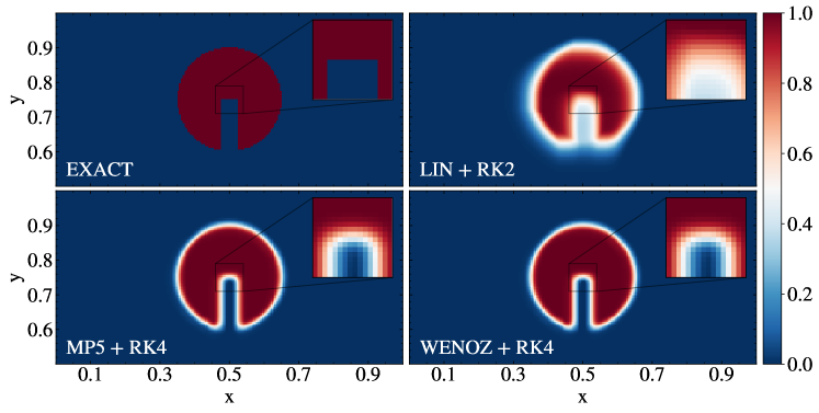
Figure 4: Plot of $v_{z}(x)$ for a 2D slotted cylinder advected for one period with $[200\times 200]$ grid points. The top left panel shows the initial condition, while the top right is the result obtained with a $2^{\rm nd}$-order method employing a LINEAR+RK2 scheme. Conversely, the bottom left and right panels show the results obtained with the novel $4^{\rm th}$-order accurate method using, respectively, the pointwise WENOZ and MP5 algorithms coupled with the RK4 integrator.

8.2 2D Isentropic Vortex

The isentropic vortex is a smooth exact solution of the 2D Euler equations.

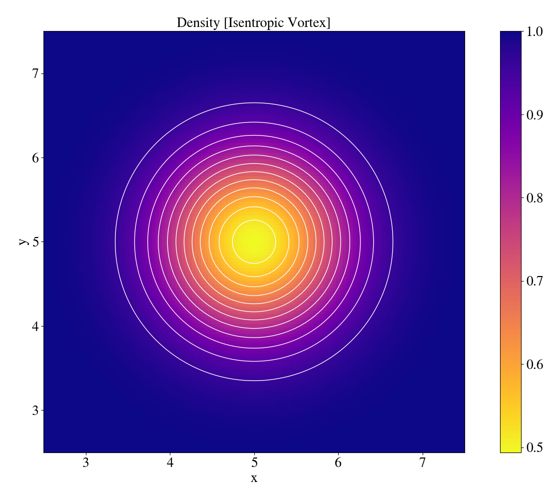
Figure 5: Plot of the density of an isentropic vortex with $256\times 256$ grid points at $t_{end}=10$ code units.

It consists of a single vortex centered at (̧5,5) in pressure equilibrium:

$$\Big{(}\delta v_{x}\,,\delta v_{y}\Big{)}=-(y_{c},\,x_{c})\frac{\epsilon}{2\pi}\exp\left(\frac{1-r_{c}^{2}}{2}\right)\,,\quad T=\frac{p}{\rho}=1-\frac{(\Gamma-1)\epsilon^{2}}{8\Gamma\pi^{2}}\exp(1-r_{c}^{2})\,,\quad s=\frac{p}{\rho^{\Gamma}}$$ (37)

where: $(x_{c},\,y_{c})=(x-5,\,y-5),\,r_{c}=\sqrt{x_{c}^{2}+y_{c}^{2}},\,\epsilon=5$ while $\Gamma=1.4$ is the adiabatic index. A constant entropy is used with value $s=1$. The vortex shifts along the main diagonal of the computational domain with uniform velocity (̧1,1) and returns in its original position after $t=10$. The domain is assumed to be periodic and its size must be taken large enough to ensure that there is no interaction between off-domain vortices.

Each simulation has run using our new WENOZ and MP5 punctual reconstructions with a domain of size: $(32\times 32)$, $(64\times 64)$, $(128\times 128)$, $(256\times 256)$ grid points, with $N^{\rm ghost}=4$. The imposed boundary conditions are periodic. The total simulation time is $t_{\rm fin}=10.0$ code units and the chosen CFL is $0.4$.

The vortex problem serves as a computational benchmark to test the accuracy of the novel numerical scheme in reproducing the vortex structure after several revolutions [54]. In Fig. 6 are reported the plots of the convergence rates produced by the novel algorithm: the plots show the trend of the convergence error evaluated as L1-norm on the initial and final density. On the top right corner are reported the expected rate of convergence, evaluated as a Linear Regression of the L1 norm as a function of $N_{grid}$, and the actual rate of convergence.

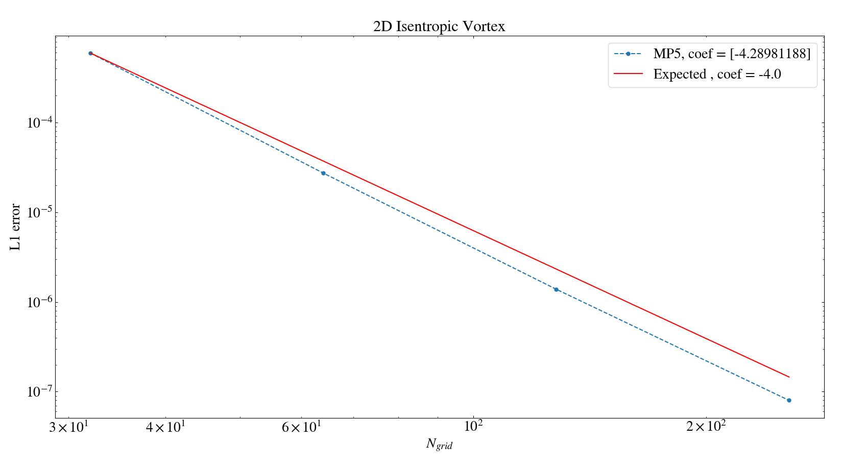
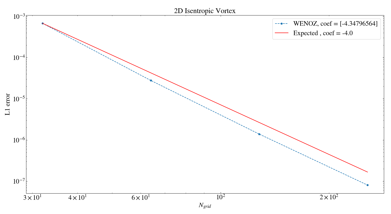
Figure 6: Plot of the 2D L1 norm vector as a function of the grid resolution for the isentropic vortex problem. Simulations have been performed with $N_{grid}=32,64,128,256$. The left panel shows the convergence plot for a RK4+MP5 scheme, while the right panel shows it for a RK4+WENOZ scheme. The L1 norm is evaluated as the averaged difference between the initial and final values of the density.

9 Numerical Tests: MHD

9.1 Circularly polarized Alfvén wave

Circularly polarized Alfvén waves are an exact, nonlinear solution to the equations of MHD. [65] introduced the propagation of these waves as a sensitive test of dispersion properties of MHD algorithms. This benchmark is proves the genuine $4^{th}$-order convergence of the upgraded scheme. This benchmark is originally conceived as a 1D test, while the 2D and 3D configurations are obtained as rotated versions of the 1D setup. Initial conditions are:

$$\rho=1,\quad\mathbf{\bf v}=\left[V_{0},\,|\epsilon|\sin(\phi),\,|\epsilon|\cos(\phi)\right],\quad\mathbf{B}=\left[1,\,\epsilon\sqrt{\rho}\sin(\phi),\,\epsilon\sqrt{\rho}\cos(\phi)\right],\quad\displaystyle P=P_{0}\,,$$ (38)

where $V_{0}$ is the translation velocity in the $x$ direction, $\phi$ is the phase ($k_{x}x$ in 1D, ($k_{x}x+k_{y}y$) in 2D) and ($k_{x}x+k_{y}y+k_{z}z$) in 3D) and $\epsilon$ is the wave amplitude ($\epsilon>0$ implies right going waves; $\epsilon<0$ implies left going waves). With this normalization, the Alfvén velocity $V_{A}=B_{x}/\sqrt{\rho}$ is always unity.

The configuration is rotated by specifying $\tan\alpha=k_{y}/k_{x}$ and $\tan\beta=k_{z}/k_{x}$ which express the ratios between the $y$- and $z$-components of the wave vector with the $x$ component. In order to apply periodic boundary conditions everywhere, an integer number of wavelegnths must be contained in each direction, that is, $k_{x}=2\pi/L_{x}$, $k_{y}=2\pi/L_{y}$, $k_{z}=2\pi/L_{z}$.

The tests uses the tools in the *rotate.c* program, which requires to specify the four integer shifts such that:

$$\tan\alpha=-\frac{j_{x}}{j_{y}}\frac{\Delta x}{\Delta y}=\frac{L_{x}}{L_{y}},\qquad\tan\beta=-\frac{k_{x}}{k_{z}}\frac{\Delta x}{\Delta z}=\frac{L_{x}}{L_{z}}$$ (39)

The final time step is one period and is found from [45]:

$$V_{A}=\omega/|k|\rightarrow 1/T=\sqrt{1+\tan^{2}\alpha+\tan^{2}\beta}$$ (40)

Tests have been performed using the novel MP5 and WENOZ punctual reconstructions schemes with either GLM or CT algorithms for DivB control. Each simulation run with a domain size of: $N_{x}$ grid points for 1D simulations, $N_{x}\times N_{x}/2$ for 2D simulations and $N_{x}\times N_{x}/2\times N_{x}/2$ grid points for 3D simulations, with $N_{x}=32,64,128,256$. The ghost zones implied were $N^{\rm ghost}=5$. The imposed boundary conditions are periodic. Rivedere questa parte perchè inesatta The total simulation time is $t_{\rm fin}=\frac{1}{3}$ code units with a CFL condition of $0.3$ for all schemes. In the following subsections are reported the convergence-error plots for 1D, 2D and 3D simulations. On the top right corner of each plot is reported the estimated convergence rate versus the expected one. The convergence rate has been evaluated as a Linear Regression of the L1 norm as a function of $N_{grid}$.

9.1.1 1D Circularly polarized Alfvén wave

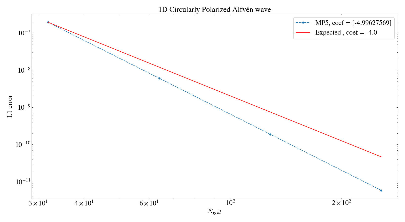
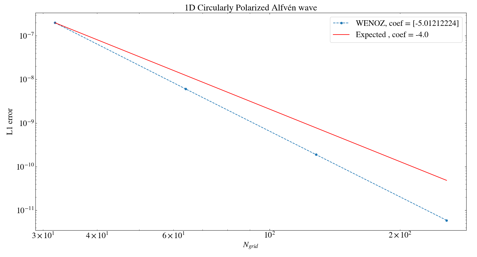
Figure 7: Plot of the 1D L1 norm vector as a function of the grid resolution for a CP Alfvén wave problem. The left panel shows the convergence plot for a RK4+MP5+CT scheme, while the right panel shows it for a RK4+WENOZ+CT scheme. The L1 norm is evaluated as the averaged difference between the initial and final values of the magnetic pressure.

9.1.2 2D Circularly polarized Alfvén wave

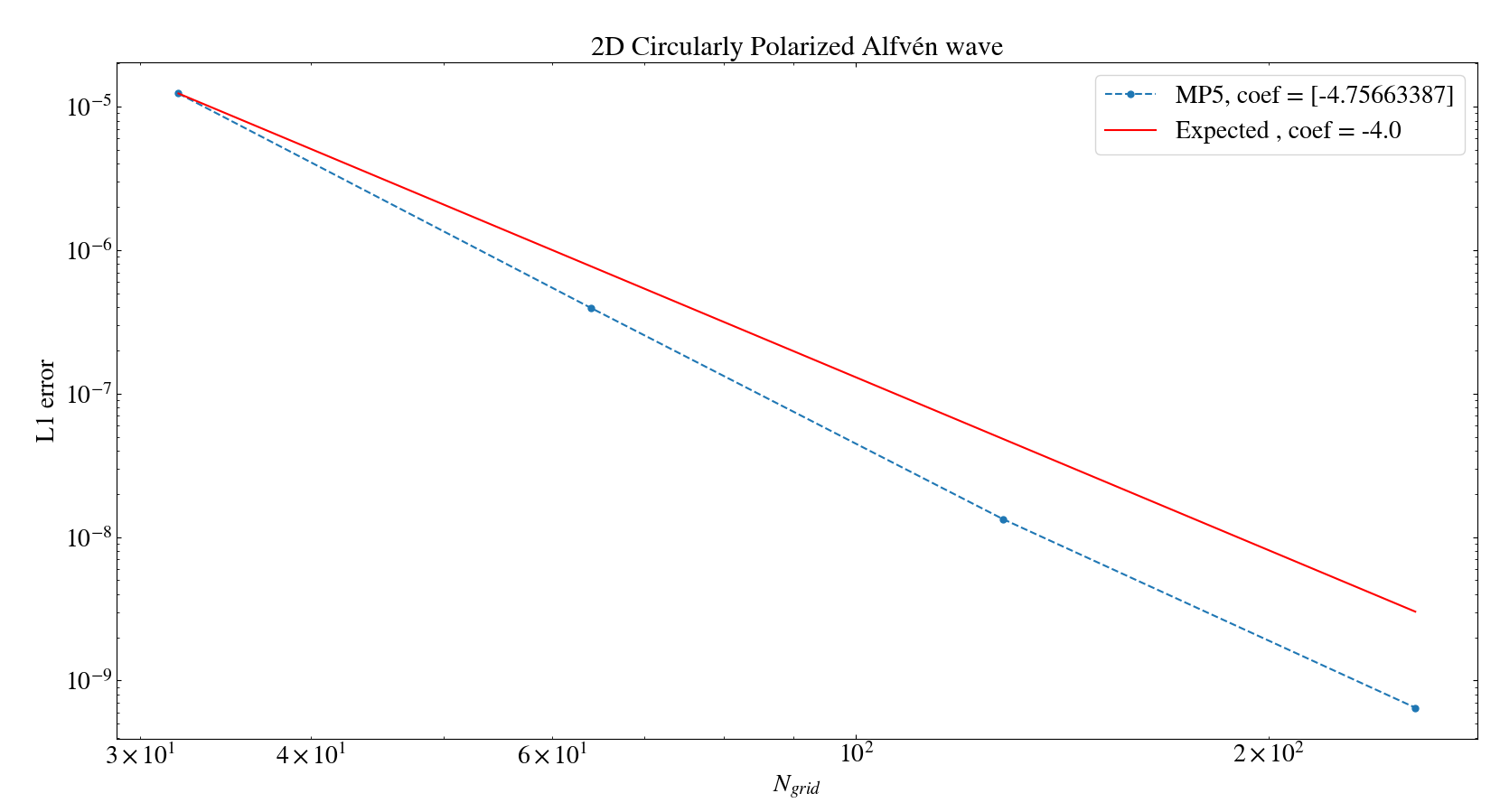
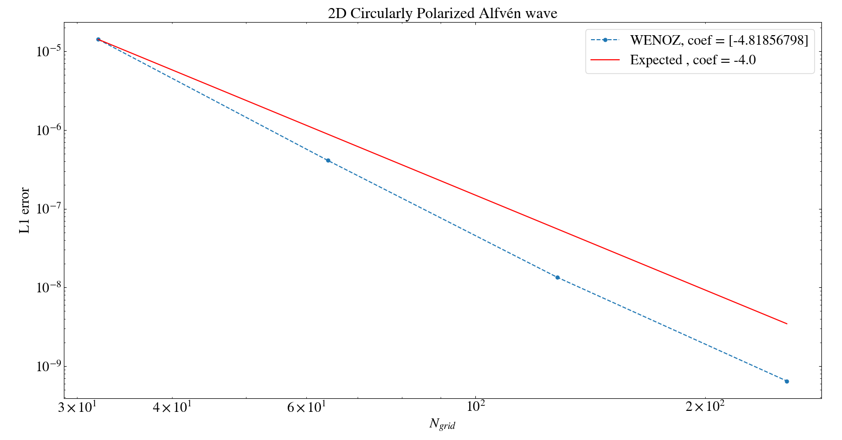
Figure 8: Plot of the 2D L1 norm vector as a function of the grid resolution for a CP Alfvén wave problem. The left panel shows the convergence plot for a RK4+MP5 scheme, while the right panel shows it for a RK4+WENOZ scheme. The L1 norm is evaluated as the averaged difference between the initial and final values of the magnetic pressure.

9.1.3 3D Circularly polarized Alfvén wave

Figure 9: Plot of the 3D L1 norm vector as a function of the grid resolution for a CP Alfvén wave problem. The left panel shows the convergence plot for a RK4+MP5 scheme, while the right panel shows it for a RK4+WENOZ scheme. The L1 norm is evaluated as the averaged difference between the initial and final values of the magnetic pressure.

For the sake of completeness, in fig. 10 are compared the convergence errors, along with the convergence rates, for a 3D circularly polarized Alfvén wave. Simulations have been carried out with a LINEAR+RK2 scheme, and with both a MP5/WENOZ+RK4 schemes.

Figure 10: Convergence error plots for a 3D circularly polarized Alfvèn wave. Simulations have been performed with a LINEAR+RK2 scheme (red line), and with both a MP5/WENOZ+RK4 scheme (blue and green lines). The expected rates are plotted near the evaluated rates as dashed grey lines. The convergence rates are reported on the top right corner.

The $4^{th}$-order method produces clear benefits in the reduction of the computational domain required at a given accuracy. In fact, while retaining the accuracy $\epsilon$:

$$\begin{cases}\displaystyle L_{1}^{2}\simeq c_{2}\Delta x_{2}^{2}=\epsilon\\ \vskip 6.0pt plus 2.0pt minus 2.0pt\cr\displaystyle L_{1}^{4}\simeq c_{4}\Delta x_{4}^{4}=\epsilon\end{cases}\Longrightarrow\qquad\displaystyle\frac{\Delta x^{2}_{2}}{\Delta x^{4}_{4}}\propto\frac{c_{4}}{c_{2}}\propto O(1)$$ (41)

Since $\Delta x\propto N_{\rm grid}^{-1}$, the number of grid points needed by the $4^{th}$-order scheme to converge at the accuracy $\epsilon$ is: $N_{4th}\simeq\sqrt{N_{2nd}}$. For an $n^{th}$-dimensional simulation the CPU-time goes as: $T\propto N^{n+1}$. In particular, for a 3D simulation: $T\propto N^{4}$. The CPU time required by each scheme goes as:

$$\begin{cases}\displaystyle T^{2nd}\simeq k_{2}N_{2}^{4}\\ \vskip 6.0pt plus 2.0pt minus 2.0pt\cr\displaystyle T^{4th}\simeq k_{4}N_{4}^{4}\end{cases}\Longrightarrow\qquad\displaystyle\frac{T^{4th}}{T^{2nd}}\simeq\frac{k_{4}}{k_{2}}(N_{4})^{-4}$$ (42)

This means that the CPU time gain endorsed by the high order scheme improves with the grid resolution and with the dimensionality of the underlying problem. All the convergence rates presented in this work demonstrate that the upgraded PLUTO code is meeting the expected improvements in CPU-time gain.

9.2 2D Field Loop Advection

This problem consists of a weak magnetic field loop being advected in a uniform velocity field. Since the total pressure is dominated by the thermal contribution, the magnetic field is essentially transported as a passive scalar. The preservation of the initial circular shape tests the scheme dissipative properties and the correct discretization balance of multidimensional terms.

Following [24] [45], the computational box is defined by $x\in[-1,1],\,y\in[-0.5,0.5]$ discretized on $2N_{y}\times N_{y}$ grid cells ($N_{y}=64$). Density and pressure are initially constant and equal to 1. The velocity of the flow is given by:

$$\mathbf{v}=V_{0}(\cos\alpha,\sin\alpha)$$ (43)

with $V_{0}=\sqrt{5},\,\sin\alpha=1/\sqrt{5},\,\cos\alpha=2/\sqrt{5}$.
The magnetic field is defined as:

$$A_{z}=\left\{\begin{array}[]{ll}A_{0}(R-r)&\textrm{if}\quad R_{1}<r\leq R\,,\\ \vskip 6.0pt plus 2.0pt minus 2.0pt\cr 0&\textrm{if}\quad r>R\,,\end{array}\right.$$ (44)

with $A_{0}=10^{-3},\,R=0.3,\,r=\sqrt{x^{2}+y^{2}}$.

Simulations have been performed on a computational domain of $256\times 128$ grid points with a LINEAR+RK2 scheme, a WENO3+RK3 scheme, and with both a MP5/WENOZ+RK4 schemes for up to $t_{fin}=2.0$ code units. The CFL was set at $0.4$ and double periodic boundary conditions are imposed.

Figure 11 shows the magnetic field lines and contours of the out-of-plane component of the current density after advection of the loop twice around the domain. The current density is particularly sensitive to diffusion or oscillations in the field.

Figure 11: Plot of the magnetic energy density for a 2D field loop advected at $t_{\rm fin}=2.0$. The magnetic field lines of the out-of-plane component are overlaid as contour lines in white.

Another extremely relevant aspect is the capability of the upgraded algorithm to reduce the numerical dissipation introduced by the code: Fig 12 shows the trend of the magnetic energy density over time for 3 simulations performed, respectively, with a $2^{nd}$-order accurate (red), a $3^{rd}$-order accurate (green), and a $4^{th}$-order accurate (blue) scheme. The magnetic energy decay is relevant for the $2^{nd}$-order scheme, while the $3^{rd}$ and $4^{th}$-order schemes demonstrate to be capable of preserving the magnetic energy throghout the simulation. As always though, the $4^{th}$ order yields the best performance.

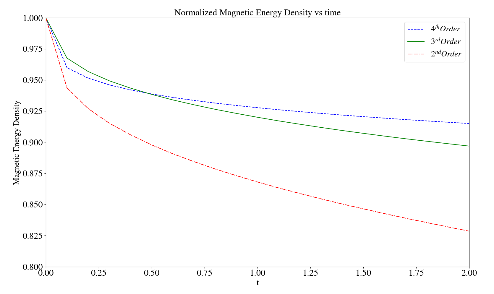
Figure 12: Plot of the magnetic energy density of a field loop advected over time. Each simulation has been performed with a $2^{nd}$-order scheme (red line), a $3^{rd}$-order scheme (green line), and a $4^{th}$-order scheme (blue line). The magnetic energy is well preserved by the novel algorithm.

Furthermore, for this particular problem, the choice of the spatial reconstruction method appears to be relevant on the conservation of the magnetic energy. Several tests have been performed using different high-order spatial reconstruction algorithms: the MP5 [62], the WENOZ [15] and the PPM [41]. The PPM appears to dissipate more, this may be due to the intrinsic architecture of the algorithm which implies the presence of a limiter that, on this and others physical problems, introduces a ”clipping” effect (namely, the reconstruction is flat whenever a minimum or a maximum are present). The clipping effect downgrades the quality of the reconstruction, resulting in a more dissipative scheme than the MP5 and WENOZ.

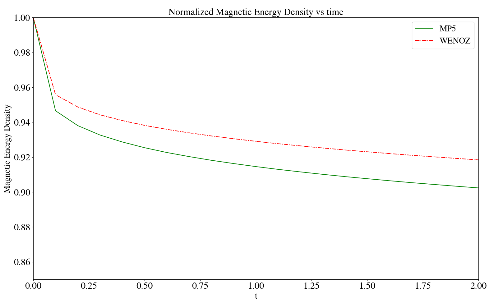
Figure 13: Plot of the magnetic energy density of a field loop advected over time. Each simulation has been performed with a $4^{th}$-order scheme with different spatial reconstruction algorithms: WENOZ (dashed line), and MP5 (blue line).

9.3 MHD Blast Wave

We run a set of simulations to infer the magnetization breakpoint in a Blast wave problem. The simulation setup is the one by Felker and Stone (2018): in this test problem, a strongly magnetized medium with uniform $B_{0}$

$$\begin{cases}B_{x}=B_{0}\sin{\theta}\cos{\phi}\\ B_{y}=B_{0}\sin{\theta}\sin{\phi}\\ B_{z}=B_{0}\cos{\theta}\end{cases}$$ (45)

of a square periodic domain spanning $\left[-0.5,0.5\right]^{2}$ is initialized with $\rho=1$ and $\gamma=\frac{5}{3}$. The ambient pressure is $P_{out}=0.1$ while an overpressure $P_{in}=10$ region is set for cells within a radius $r=0.1$ of the origin. The magnetic angles tested are $\phi=\left\{0.0^{\circ},45.0^{\circ}\right\},\theta=90.0^{\circ}$.

Fig. 14 shows the density, pressure, magnetic pressure and specific kinetic energy of a blast wave at $t_{end}=0.15$ with $B_{0}=1.0$, $\phi=45.0^{\circ}$, $400^{2}$ grid points, a $CFL=0.4$ and Outflow boundary conditions obtained with the high-order module of the PLUTO code. As we can see the magnetic field is providing a perturbation that is oriented towards the diagonal of an ideal medium with infinite electrical conductivity.

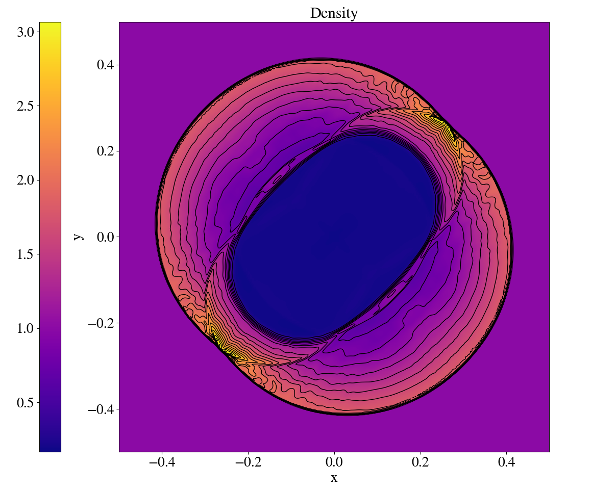
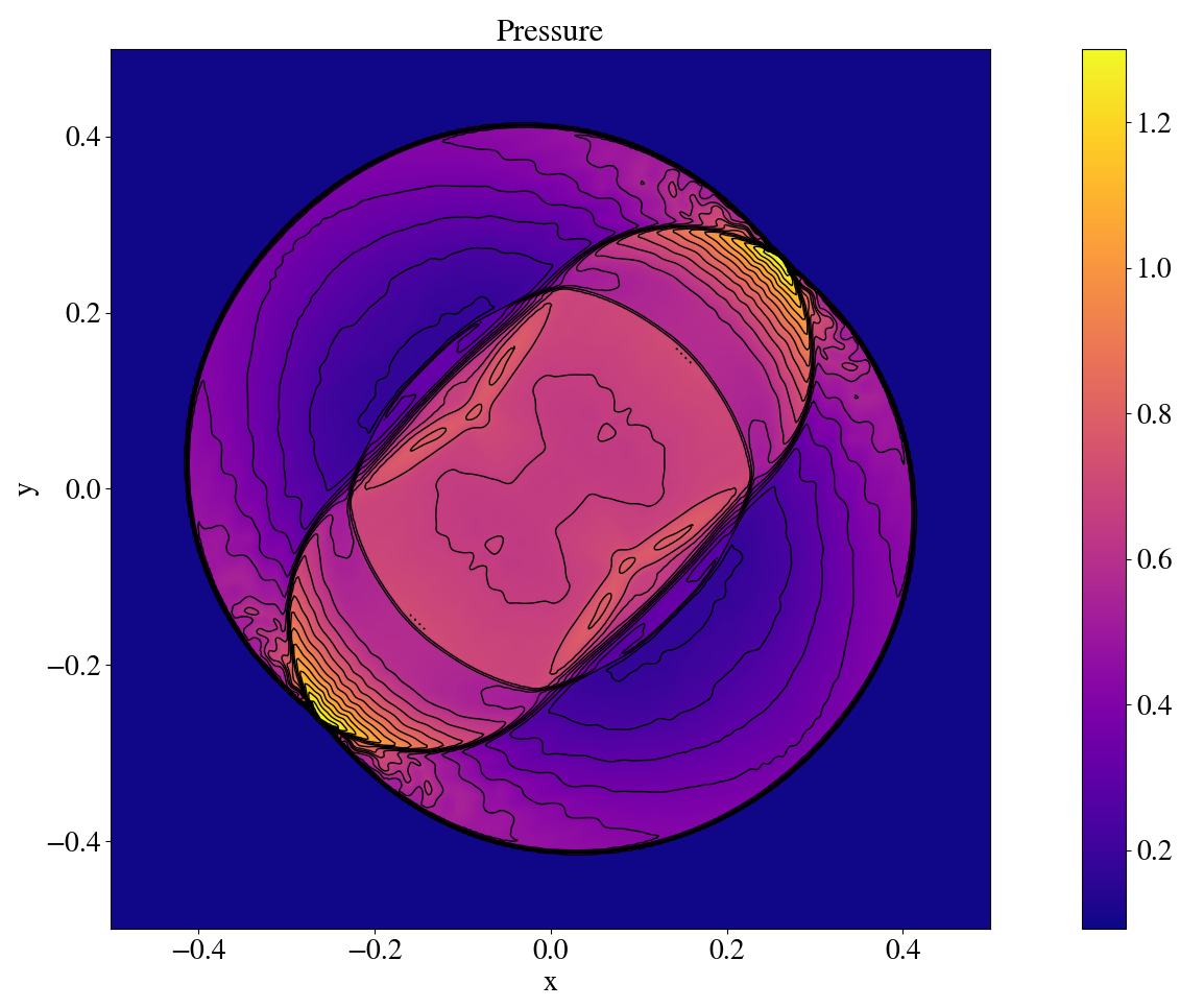
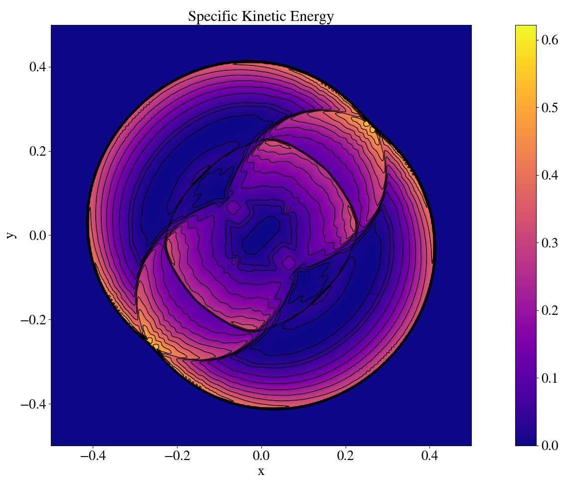
Figure 14: Plots for the density, pressure, magnetic pressure and specific kinetic energy of an MHD Blast wave at $t_{end}=0.15$. The magnetic field was set to $B_{0}=1$ in a medium with $\rho=1$. An initial pressure gradient with $P_{in}=10.0$ and $P_{out}=0.1$ triggers the explosion. The simulations were performed in a domain of $[400^{2}]$ gird points, and here are plotted with 20 black contour lines.

To search for the magnetization breakpoint, we selected the limiter described in Sec.7 and run a set of simulations with PRECONSTRUCT = $\left\{YES,NO\right\}$, RECONSTRUCTION = $\left\{WENOZ,MP5\right\}$, RES = $\left\{100^{2},200^{2},400^{2}\right\}$ grid points. We adopted a bisection-like method to search for the breakpoint with $B_{0}\in\left[0.0,3.0\right]$

The results obtained are:

• PRECONSTRUCT = YES, REC = WENOZ, RES = 200, $\phi=45.0$, $B_{lim}=1.2114$

• PRECONSTRUCT = NO , REC = WENOZ, RES = 200, $\phi=45.0$, $B_{lim}=1.2088$

• PRECONSTRUCT = YES, REC = MP5 , RES = 200, $\phi=45.0$, $B_{lim}=1.2083$

• PRECONSTRUCT = NO , REC = MP5 , RES = 200, $\phi=45.0$, $B_{lim}=1.2029$

• PRECONSTRUCT = YES, REC = WENOZ, RES = 200, $\phi=0.0$, $B_{lim}=1.2116$

• PRECONSTRUCT = NO , REC = WENOZ, RES = 200, $\phi=0.0$, $B_{lim}=1.2088$

• PRECONSTRUCT = YES, REC = MP5 , RES = 200, $\phi=0.0$, $B_{lim}=1.2086$

• PRECONSTRUCT = NO , REC = MP5 , RES = 200, $\phi=0.0$, $B_{lim}=1.2033$

• PRECONSTRUCT = YES, REC = WENOZ, RES = 100, $\phi=45.0$, $B_{lim}=1.2076$

• PRECONSTRUCT = YES, REC = WENOZ, RES = 400, $\phi=45.0$, $B_{lim}=1.2099$

We can conclude that the breakpoints found for each configurations are consistent since we are expecting the breakpoint not to be dependent on the reconstruction method.

9.4 The Orszag-Tang vortex

The Orszag-Tang vortex problem is a popular benchmark to prove the robustness of the MHD schemes, although no exact solution exists. This test consist of an initial vorticity distribution that spins the fluid clockwise leading to the steepening of density perturbations into shocks. The dynamics is then regulated by multiple shock-vortex interactions leading to the formation of a horizontal current sheet at the center of the domain. Here magnetic energy is gradually dissipated and the current sheet twists leading to the structures observed in Fig. 15. The most noticeable feature lies at the center of the computational domain where the formation of a magnetic island (an O-point) can be discerned when using the $4^{th}$-order scheme. The presence of the central island may be attributed to the amount of numerical resistivity that can trigger tearing-mode reconnection episodes across the central current sheet, resulting in a final merging in this larger island. The turbulence that results in this problem tests the ability of the numerical method to resolve the MHD shock-shock interactions while strictly suppressing the onset of magnetic monopoles. Here, the situation is highly dynamic with the central current sheet undergoing a fast thinning process induced by converging shock fronts, and it is known that only in the presence of a sufficiently high local Lundquist number (i.e. low numerical dissipation in the ideal MHD case of the test) the tearing instability is expected to develop on the ideal (Alfvénic) timescales, see [34] and [50].

The initial condition accounts for constant densities and pressure: $\rho_{0}=\frac{25}{9}$, $p_{0}=\frac{5}{3}$ in a periodic domain of size $[L_{x},L_{y}]=[0,2\pi]$, with an initial velocity $(v_{x},v_{y})=(-\sin{y},\sin{x})$. The magnetic field is computed as: $(B_{x},B_{y})=(-\sin{y},\sin{2x})$.

Simulations have been performed using the WENOZ+Constrained Transport within a domain of size ($N_{x}=N_{y}=512$). The CFL number was chosen to be $0.4$ and the simulation run up to $t_{fin}=6.2$ code units. Figure 15 shows the development of the density, pressure, specific kinetic energy and magnetic energy of the vortex.

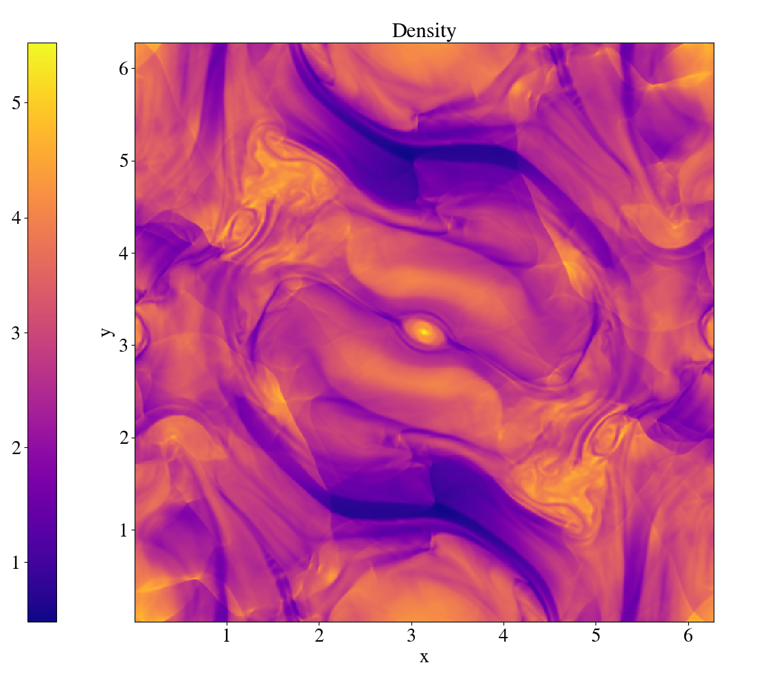
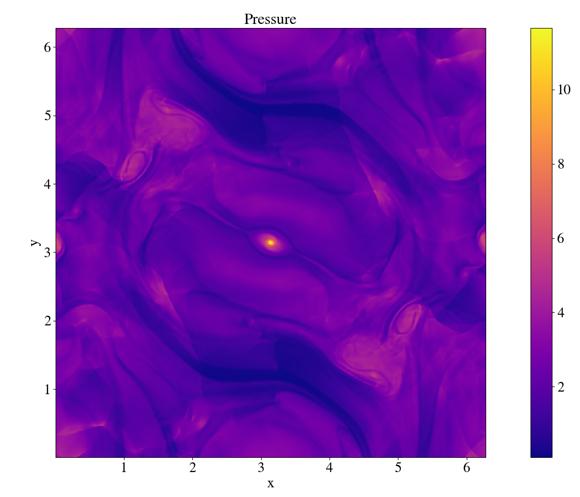
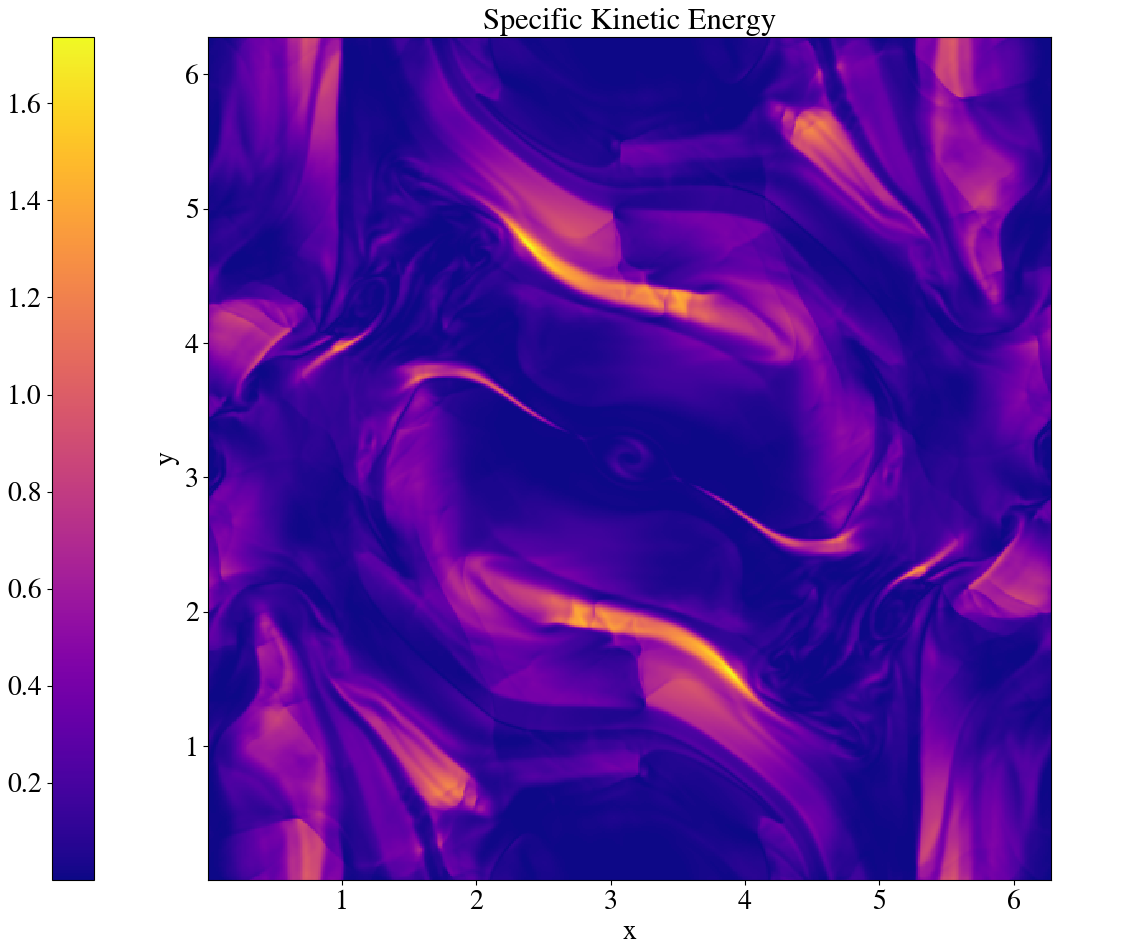
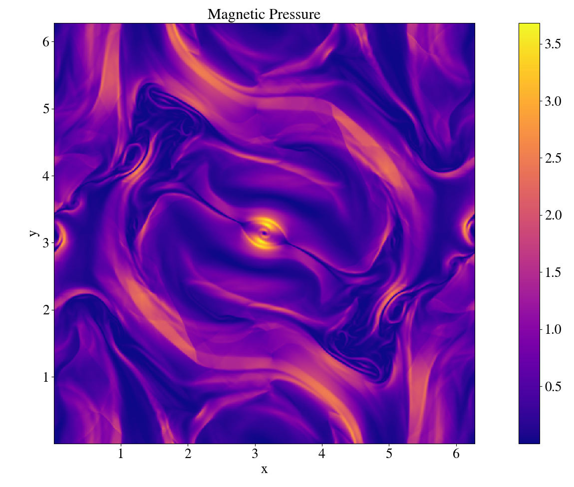
Figure 15: From top-left to bottom right: density, pressure, specific kinetic energy and magnetic pressure of the Orszag-Tang vortex at the final time ($t_{\rm fin}=6.2$ code units) for a simulation with $512\times 512$ grid cells.

10 Bibliographic research

This section summarizes some relevant published works.

10.1 NC Geometries

Zhang et al. 2019 ApJS: relevant work on 3D FV MHD schemes using Non-Orthogonal Curvilinear Geometries.

Relevant ideas:

• Basic cell structure in the FV solver is a general hexahedron without the requirement of coordinate orthogonality but the grid structure is logically Cartesian in the computational space. In the GAMERA code, cell-centered vector components represented as Cartesian fields in order to avoid source terms originating from curvilinear coord. Cartesian components of the cell-centered velocity $(u_{x},u_{y},u_{z})$ and magnetic field vectors $B_{x},B_{y},B_{z}$ are defined in the “Base Cartesian Coordinate System.”

• Variation of grid geometry is taken into account in the reconstruction process (12th-order Gaussian quad). At cell interfaces upwind reconstruction is done using the primitive method with an 8 point stencil (no PPM, no MP5, no WENO). After interf rec of the Cartesian velocity and B field, coordinate transforms at the cell interfaces are needed to rotate the left and right velocity and B field from the base Cartesian coordinate system $(x,y,z)$ into the face-normal coordinate system $(x_{n},x_{1},x_{2})$, to evaluate fluxes.

• CT based on the Yee-Grid (Yee 1966) adaptation to non-orthogonal geometries. Staggered grid, magnetic fluxes evolved using cell-edge-centered E fields recovered from averaged B and v reconstructed at edges. Calculation of E is a Rusanov scheme adapted to a cell corner $E=-v\times B_{avg}$. v and B are not in the same Coord System (CS) v is in the base Cartesian CS, $B_{avg}$ is in a local non-orthogonal CS. To calculate the cross product define a new orthogonal CS $(e_{1},e_{2},e_{z})$ with one axis $e_{z}$ aligned with the direction of the cell edge, and transform into the new CS.

• Compute the cell-centered B field using FC magnetic fluxes by considering the volume integral of $\mathbf{\nabla}\cdot\mathbf{rB}$ over V.

Numerical Tests: Cartesian and non-Cartesian slotted cylinder, field-loop advection, circularly polarized nonlinear Alfvén waves, Orszag–Tang vortex and spherical blast waves in strong magnetic fields.

10.2 High-Order Codes

Verma et al. 2018 MNRAS: $4^{th}$-order accurate FV CWENO schemes for MHD problems on Cartesian meshes.

• CT scheme, dimension-by-dimension approach employing a 1D fourth-order accurate CWENO (1D-CWENO4) reconstruction polynomial, convolutions by Laplacian operators (as in McCorquodale&Colella 2011 and FelkerStone 2018) + 4th-SSPRK method.

• Reconstruction of area averages from volume averages before reconstructing interfaces (why needed?)

• Strong Stability-Preserving Runge–Kutta (SSPRK) method is used (Shu 2009). The SSPRK method used in this paper is a ten-stage fourth-order method, described in Ketcheson (2008).

References

- [1] M. Abramowitz, I. A. Stegun, Handbook of Mathematical Functions, 1964
- [2] Anile, M. 1989, ”Relativistic fluids and magneto-fluids”, Cambridge University press
- [3] M. Anjiri, A. Mignone, G. Bodo, P. Rossi, 2014 MNRAS, 442,3, 11, 2228–2239,
- [4] Appl S., Lery T., Baty H., 2000, A&A, 355, 818
- [5] Pierre Auger Collaboration, J. Abraham, P. Abreu, M. Aglietta, C. Aguirre, D. Allard, I. Allekotte, J. Allen, P. Allison, C. Alvarez, and et al. Correlation of the Highest-Energy Cosmic Rays with Nearby Extragalactic Objects. Science, 318:938, 2007.
- [6] X.-N. Bai, D. Caprioli, L. Sironi, and A. Spitkovsky. Magnetohydrodynamic-particle- in-cell Method for Coupling Cosmic Rays with a Thermal Plasma: Application to Non-relativistic Shocks. apj, 809:55, 2015.
- [7] D.S. Balsara, J. Kim, A comparison between divergence-cleaning and staggered-mesh formulations for numerical magnetohydrodynamics, ApJ 602 (2004) 1079.
- [8] D. Band, J. Matteson, L. Ford, B. Schaefer, D. Palmer, B. Teegarden, T. Cline, M. Briggs, W. Paciesas, G. Pendleton, G. Fishman, C. Kouveliotou, C. Meegan, R. Wilson, and P. Lestrade. BATSE observations of gamma-ray burst spectra. I - Spectral diversity. apj, 413:281, 1993.
- [9] Bateman G., 1980, MHD Instabilities. MIT Press, Cambridge
- [10] J. H. Beall. A Review of Astrophysical Jets. XI Multifrequency Behaviour of High Energy Cosmic Sources Workshop (MULTIF15), 2015.
- [11] O. Bromberg, C. B. Singh, J. Davelaar, and A. A. Philippov, “Kink instability: Evolution and energy dissipation in relativistic force-free nonrotating jets,” The Astrophysical Journal, vol. 884, p. 39, oct 2019.
- [12] R. Blandford and D. Eichler. Particle acceleration at astrophysical shocks: A theory of cosmic ray origin. physrep, 154:1, 1987.
- [13] G. Bodo, G. Mamatsashvili, P. Rossi and A. Mignone, (2013) MNRAS, 434, 3030
- [14] Bodo G., Massaglia S., Rossi P., Rosner R., Malagoli A., Ferrari A., 1995, AA, 303, 281
- [15] R. Borges, M. Carmona, B. Costa, W.S. Don, An improved weighted essentially non-oscillatory scheme for hyperbolic conservation laws, J. Comput. Phys. 227 (2008) 3191–3211.
- [16] C. Chiuderi and M. Velli. Basics of Plasma Astrophysics. 2015.
- [17] Z. Dai, F. Daigne, and P. Mészáros. The Theory of Gamma-Ray Bursts. ssr, 212:409, 2017.
- [18] A. Dedner, F. Kemm, D. Kröner, C.D. Munz, T. Schnitzer, M. Wesenberg, Hyperbolic divergence cleaning for the MHD equations, J. Comput. Phys. 175 (2002) 645-673.
- [19] L. Del Zanna, N. Bucciantini, P. Londrillo, ”An efficient shock-capturing central-type scheme for multidimensional relativistic flows”, AA, 397-413 (2003)
- [20] D. Eichler, “Magnetic Confinement of Jets,” vol. 419, p. 111, Dec. 1993.
- [21] Fanaroff, B. L., Riley, J. M. 1974, MNRAS, 167, 31P
- [22] Felker, K. G., Stone, J. M. JCP, 375 (2018), 1365-1400
- [23] B. M. Gaensler and P. O. Slane. The Evolution and Structure of Pulsar Wind Nebulae. araa, 44:17, 2006.
- [24] Gardiner, T. A., Stone, J. M. 2005a, J. Comput. Phys., 205, 509
- [25] D. Giannios, 2010, Monthly Notices of the Royal Astronomical Society: Letters, Volume 408, Issue 1, Pages L46–L50
- [26] D. Giannios. Acceleration and emission of MHD driven, relativistic jets. 283:012015, 2011.
- [27] Godunov, S. K. 1959, Matematicheskii Sbornik, 47, 271
- [28] S.Gottlieb, C. W. Shu, E. Tadmor, Strong stability-preserving High-order time dis- cretization methods, SIAM Vol. 43 No. I, pp. 89-112;
- [29] Guzik,S. M., Gao, X., Owen, D. L., McCorquodale, P., Colella, P., Comput. Fluids 123 (2015) 202–217
- [30] G.S. Jiang, C.-W. Shu, Efficient implementation of weighted ENO schemes, J. Comput. Phys. 126 (1996) 202–228.
- [31] H. Krawczynski and E. Treister. Active galactic nuclei - the physics of individual sources and the cosmic history of formation and evolution. Frontiers of Physics, 8, 2013.
- [32] L. Isherwood, S. Gottlieb, Z. Grant, Strong Stability Preserving Integrating Factor Runge–Kutta Methods. SIAM Journal on Numerical Analysis 56(6) (2018), pp. 3276–3307.
- [33] L. D. Landau and E. M. Lifshitz. Fluid mechanics. 1959
- [34] S. Landi, L. Del Zanna, E. Papini, F. Pucci, M. Velli, Resistive magnetohydrodynamics simulations of the ideal tearing mode, Astrophys. J. 806 (1) (2015) 131
- [35] G. Lapenta. Particle simulations of space weather. Journal of Computational Physics, 231:795, 2012.
- [36] Lax P., Wendroff B., 1960, Comm. Pure Appl. Math., 13, 217
- [37] LeVeque R., 1992, Numerical Methods for Conservation Laws, 2nd edn. Birkhäuser, Bern
- [38] Loffeld, J., Hittinger, J.A.F., Int. J. High Perform. Comput. Appl. (2017)
- [39] M. S. Longair. High Energy Astrophysics. 2011.
- [40] N. F. Loureiro and D. A. Uzdensky. Magnetic reconnection: from the Sweet-Parker model to stochastic plasmoid chains. Plasma Physics and Controlled Fusion, 58:014021, 2016.
- [41] McCorquodale Colella, Commun. Appl. Math. Comput. Sci. 6 (1) (2011) 1–25
- [42] Mignone A., Bodo G., Massaglia S., Matsakos T., Tesileanu O., Zanni C., Ferrari A., 2007, ApJS, 170, 228
- [43] Mignone A., Rossi P., Bodo G., Ferrari A., Massaglia S., 2010, MNRAS, 402, 7
- [44] A. Mignone, P. Tzeferacos, A second order unsplit Godunov scheme for cell-centered MHD: the CTU–GLM scheme, ApJS 229 (2010) 2117–2138.
- [45] A. Mignone, P. Tzeferacos., G.Bodo, High-order conservative finite difference GLM–MHD schemes for cell-centered MHD, JCP, 229 (2010) 5896–5920
- [46] Y. Mizuno, Y. Lyubarsky, K.-I. Nishikawa, and P. E. Hardee, “Three- Dimensional Relativistic Magnetohydrodynamic Simulations of Current-Driven Instability. I. Instability of a Static Column,” vol. 700, pp. 684–693, July 2009.
- [47] S. M. O’Neill, K. Beckwith, and M. C. Begelman, “Local simulations of insta- bilities in relativistic jets – I. Morphology and energetics of the current-driven instability,” Monthly Notices of the Royal Astronomical Society, vol. 422, pp. 1436–1452, 04 2012.
- [48] Steven A. Orszag, Cha-Mei Tang, Small-scale structure of two-dimensional magnetohydrodynamic turbulence, J. Fluid Mech. 90 (01) (1979) 129
- [49] D. E. Osterbrock and G. J. Ferland. Astrophysics of gaseous nebulae and active galactic nuclei. 2006.
- [50] E. Papini, S. Landi, L. Del Zanna, Fast magnetic reconnection: secondary tearing instability and role of the hall term, Astrophys. J. 885 (1) (2019) 56
- [51] Roe, P. L. 1986, Ann. Rev. Fluid Mech., 18, 337
- [52] G. B. Rybicki and A. P. Lightman. Radiative Processes in Astrophysics. 1986.
- [53] Shu C.-W., 2009, SIAM Rev., 51, 82
- [54] C.W. Shu, ”High-order Finite Difference and Finite Volume WENO Schemes and Discontinuous Galerkin Methods for CFD”, ICASE Report No.2001-11, NASA/CR-2001-210865
- [55] L. Sironi and A. Spitkovsky. Particle Acceleration in Relativistic Magnetized Collisionless Pair Shocks: Dependence of Shock Acceleration on Magnetic Obliquity. apj, 698:1523, 2009.
- [56] L. Sironi, A. Spitkovsky, and J. Arons. The Maximum Energy of Accelerated Particles in Relativistic Collisionless Shocks. apj, 771:54, 2013.
- [57] Lorenzo Sironi and Anatoly Spitkovsky 2014 ApJL 783 L21
- [58]
- [59] R. J. Spiteri and S. J. Ruuth, A new class of optimal high-order strong-stability-preserving time discretization methods, SIAM Journal on Numerical Analysis, 40 (2002), pp. 469–491.
- [60] James M. Stone, Thomas A. Gardiner, Peter Teuben, J.F. Hawley, J.B. Simon, Athena: a new code for astrophysical MHD, Astrophys. J. Suppl. Ser. 178 (2008) 137–177 E. Striani, A. Mignone, B. Vaidya, G. Bodo, and A. Ferrari. MHD simulations of three-dimensional resistive reconnection in a cylindrical plasma column. mnras, 462:2970, 2016.
- [61] Errol J. Summerlin and Matthew G. Baring 2012 ApJ 745 63
- [62] A. Suresh, H.T. Huynh, Accurate monotonicity-preserving schemes with Runge–Kutta time stepping, J. Comput. Phys. 136 (1997) 83–99.
- [63] Toro, E. F. 1997, Riemann Solvers and Numerical Methods for Fluid Dynamics, Springer-Verlag, Berlin
- [64] M. Torrilhon, Locally Divergence-Preserving Upwind Finite Volume Schemes for Magnetohydrodynamics Equations, Siam J. Sci. Comput. 26 (2005) 1166
- [65] G. Tóth, The ∇ · B = 0 constraint in shock-capturing magnetohydrodynamics codes, J. Comput. Phys. 161 (2000) 605
- [66] van Leer B., 1979, J. Comput. Phys., 32, 101
- [67] A. Weinstein. Pulsar Wind Nebulae and Cosmic Rays: A Bedtime Story. Nuclear Physics B Proceedings Supplements, 256:136, 2014.
- [68] Woodward P., Colella P., 1984, J. Comput. Phys., 54, 115