Trimmed Mean Group Estimation of Average Treatment Effects in Ultra Short $T$ Panels under Correlated Heterogeneity

Abstract

Under correlated heterogeneity, the commonly used two-way fixed effects estimator is biased and can lead to misleading inference. This paper proposes a new trimmed mean group (TMG) estimator which is consistent at the irregular rate of $n^{1/3}$ even if the time dimension of the panel is as small as the number of its regressors. Extensions to panels with time effects are provided, and a Hausman-type test of correlated heterogeneity is proposed. Small sample properties of the TMG estimator (with and without time effects) are investigated by Monte Carlo experiments and shown to be satisfactory and perform better than other trimmed estimators proposed in the literature. The proposed test of correlated heterogeneity is also shown to have the correct size and satisfactory power. The utility of the TMG approach is illustrated with an empirical application.

Keywords: Correlated heterogeneity, irregular estimators, two-way fixed effects, FE-TE, tests of correlated heterogeneity, calorie demand

JEL Classification: C21, C23

1 Introduction

Fixed effects estimation of average treatment effects has been predominantly utilized for program and policy evaluation. For static panel data models where slope heterogeneity is uncorrelated with treatment effects, standard fixed and time effects (FE-TE) estimators are consistent and if used in conjunction with robust standard errors lead to valid inference in short $T$ (time dimension) panels when the number of cross sections ($n$) is sufficiently large. However, when the slope heterogeneity is correlated with the treatment and/or control variables the FE-TE estimators (also known as two-way fixed effects) become inconsistent even if both $T$ and $n\rightarrow\infty$. Such correlated heterogeneity arises endogenously in the case of dynamic panel data models considered by Pesaran and Smith (1995) even if the slope heterogeneity itself is purely random.

In the case of static panels, correlated heterogeneity could arise when treatment effects are correlated with the treatment itself and/or the control variables. For example, in estimation of returns to education, the choice of educational level is likely to be correlated with expected returns to education. In a review of active policies in labor markets, Crépon and Van Den Berg (2016) emphasize that when estimating the average impacts on workers’ productivity and earnings, correlated heterogeneity should be accounted for, to better encourage enrollment in training programs. Banerjee et al. (2015) also consider identification and estimation of heterogeneous treatment effects in the case of micro-credit evaluation programs, and Bastagli et al. (2019) consider similar issues in studies of anti-poverty cash transfer programs. In a recent survey de Chaisemartin and D’Haultfoeuille (2023) highlight the importance of allowing for correlated heterogeneity and draw attention to the misleading inferences that can result when FE-TE estimates are used in the case of heterogeneous policy effects.

Pesaran and Smith (1995) proposed mean group (MG) estimation for dynamic heterogeneous panel data models, where by construction represent examples of correlated heterogeneity. It was later shown that for panels with strictly exogenous regressors, the MG estimator is $\sqrt{n}$-consistent in the presence of correlated heterogeneity even if $T$ is fixed as $n\rightarrow\infty$, so long as $T$ is sufficiently large such that at least second order moment of the MG estimator exists. However, when $T$ is ultra short such that $T$ is close to the number of regressors, $k$, the MG estimator could fail. As shown by Chamberlain (1992) one needs $T$ to be strictly larger than $k$ for regular identification of average effects under correlated heterogeneity. Chamberlain (1992) calculated efficiency bounds for models defined by conditional moment restrictions with a nonparametric component, and proposed a $\sqrt{n}$-consistent Generalized Method of Moments (GMM) estimator for the mean of correlated random coefficients in panel data models provided that certain rank and moment conditions hold. See also Bonhomme (2012) and Arellano and Bonhomme (2012). Assuming the errors follow autoregressive moving average processes, Arellano and Bonhomme (2012) provide rank conditions under which the GMM estimators they propose for variances and densities of correlated random coefficients can be regularly identified.

The above papers adopt the GMM approach to address identification and estimation of average treatment effects. Some researchers consider other regular estimators by imposing additional restrictions on the correlation between heterogeneous coefficients and regressors. Wooldridge (2005) proposes an alternative estimator for models with nonlinear individual-specific unobserved effects, where he imposes a condition that random coefficients are mean independent of the idiosyncratic deviations in regressors. To estimate the average effects of binary treatment variables for the sub-population with no time variations in treatment status, Verdier (2020) explicitly models selection into treatment. Assuming random coefficients are independent of regressors, Lee and Sul (2022) apply a double-sided trimming scheme to the MG estimators for static panels with common correlated effects developed by Chudik and Pesaran (2015), so as to eliminate effects of outlying individual estimates with too small or too large regressor sample variances.

This paper considers identification and estimation of average treatment effects in ultra short linear panel data models with continuous covariates, where $T$ could be as small as $k$. Building on the pioneering work of Chamberlain (1992), Graham and Powell (2012) focus on panels with $T=k$, where identification issues of time effects and the mean coefficients arise especially when there are insufficient within-individual variations for some regressors. They derive an irregular estimator of the mean coefficients by excluding individual estimates from the estimation of the average treatment effects if the sample variance of regressor in question is smaller than a given threshold. Exploiting the sub-population of “stayers”with no time variations in regressors, they then propose an estimator of time effects. More recently Sasaki and Ura (2021) propose an alternative procedure to deal with the possibility of many stayers and/or slow movers in the panel. They consider various distributions of within-variations and use local polynomial regressions to provide robust inference.

In this paper, we first derive asymptotic properties of MG and FE estimators in large $n$ and short $T$ heterogeneous static panel data models, and provide sufficient conditions under which MG and FE estimators are regular, in the sense that they are $\sqrt{n}$-consistent. In cases where these conditions are not met, we propose a new trimmed mean group (TMG) estimator which makes use of additional information on trimmed units not exploited by Graham and Powell (2012). In effect, information on all units (whether subject to trimming or not) are included in the computation of the average treatment effect. Following the literature, the decision on whether a unit $i$ is subject to trimming is made with respect to the determinant of the sample covariance matrix of the regressors, denoted by $d_{i}$, and the individual estimates for unit $i$ are trimmed uniformly if $d_{i}<a_{n}=\bar{d}_{n}n^{-\alpha}$, where $\bar{d}_{n}=n^{-1}\Sigma_{i=1}^{n}d_{i}$, and $\alpha$ measures the rate of trade-off between bias and variance of TMG. Our asymptotic derivations suggest setting $\alpha$ close to $1/3$. Also noting that $d_{i}/\bar{d}_{n}$ is scale free, our choice of trimming threshold, $a_{n}$, does not involve any other tuning parameters.

We also consider heterogeneous panels with time effects and develop two new estimators of the average treatment effects in two-way fixed effects regressions, which we denote by TMG-TE and TMG-C, corresponding to cases where $T\geq k$ and $T>k$, respectively. The TMG-TE estimator is based on joint estimation of time and average effects, whilst the TMG-C estimator follows Chamberlain (1992) and eliminates the time effects before estimating the average treatments, which is possible only if $T>k$. We derive the asymptotic distributions of TMG-TE and TMG-C estimators under fairly general assumptions but require the identifying condition that the non-zero dependence between heterogeneous slope coefficients and the regressors is time-invariant. Note that this condition trivially holds in the case of FE-TE estimators whose validity requires zero dependence between the slope coefficients and the regressors.

As noted above the presence of heterogeneity by itself does not invalidate the use of the FE-TE estimator which continues to have the regular convergence rate of $\sqrt{n}$. The problem arises when slope heterogeneity is correlated with the covariates, such as the treatment variable. It is, therefore, important that before using the FE-TE estimator the assumption of uncorrelated heterogeneity is tested. To this end, we also propose Hausman-type tests of correlated heterogeneity by comparing the FE and FE-TE estimators with the associated TMG estimators, and derive their asymptotic distributions under fairly general conditions. The earlier Hausman tests of slope homogeneity developed by Pesaran et al. (1996) and Pesaran and Yamagata (2008) are based on the difference between FE and MG estimators and do not apply when $T$ is ultra short.

We also carry out an extensive set of Monte Carlo (MC) simulations to investigate the small sample properties of the TMG, TMG-TE and TMG-C estimators and how they compare with other estimators, including the trimmed estimators proposed by Graham and Powell (GP) and Sasaki and Ura (SU). The MC evidence on the size and empirical power of the Hausman-type tests of correlated heterogeneity in panel data models without and with time effects is provided, and the sensitivity of estimation results to the choice of the trimming threshold parameter, $\alpha$, is also investigated. The MC and theoretical results of the paper are all in agreement. The TMG and TMG-TE estimators not only have the correct size but also achieve better finite sample properties compared with other trimmed estimators across a number of experiments with different data generating processes, allowing for heteroskedasticity (random and correlated), error serial correlations, and regressors with heterogeneous dynamics and interactive effects. The simulation results also confirm that the Hausman-type tests based on the difference between FE (FE-TE) and TMG (TMG-TE) estimators have the correct size and power against the alternative of correlated heterogeneity.

As an empirical illustration, we re-visit the example considered by GP who provide estimates of the average effect of household expenditures on calorie demand using a balanced panel of $n=1,358$ households in poor rural communities in Nicaragua over the years 2001–2002 $(T=2)$ and 2000–2002 $(T=3)$. Comparing the FE and TMG estimates, for panels with and without time effects, we find that the Hausman tests reject the null of uncorrelated heterogeneity, thus shedding doubt on the use of FE or FE-TE estimates for this application. For the ultra short panel with $T=2$, the FE and TMG estimates of the average treatment effects are $0.6568$ $(0.0287)$ and $0.5623$ $(0.0425)$. The figures in brackets are standard errors. Given the result of the Hausman test, most likely the FE estimate is biased upward, with a much lower standard error. These results do not change if we allow for time effects. Turning to the other trimmed estimators, the GP and SU estimates, $0.4549$ $(0.1003)$ and $0.6974$ $(0.1689)$, respectively, are wide apart, and both have larger standard errors as compared to the TMG estimate. Again these estimates are not much affected by allowing for time effects. But once we consider the panel with $T=3$ the TMG and GP estimates (with or without time effects) become very similar, although the TMG estimates continue to be more precisely estimated. The gap between FE and TMG estimates also becomes closer but remains statistically highly significant.

The rest of the paper is organized as follows. Section 2 sets out the heterogeneous panel data model and investigates the asymptotic properties of the MG and FE estimators. Section 3 considers ultra short $T$ panels and discusses the need for trimming as suggested by GP. The proposed TMG estimator is introduced in Section 4, and its asymptotic properties are established in Section 5. Section 6 extends the TMG estimation to ultra short panel data models with time effects, distinguishing between cases where $T\geq k$ and $T>k$. Section 7 sets out the Hausman-type test of correlated heterogeneous slope coefficients. Section 8 describes the Monte Carlo experiments and reports the simulation results. Section 9 presents the empirical illustration. Section 10 concludes. The online supplement develops the test of correlated heterogeneity for panels with time effects, and provides supplementary information on Monte Carlo designs and additional Monte Carlo evidence.

2 Heterogeneous linear panel data models

Consider the panel data model where the outcome variable $y_{it}$ for unit $i$ at time $t$ is explained linearly in terms of the $k\times 1$ vector of covariates $\boldsymbol{w}_{it}$

$$y_{it}=\boldsymbol{\theta}_{i}^{\prime}\boldsymbol{w}_{it}+u_{it}\text{, for }i=1,2,...,n\text{, and }t=1,2,...,T,$$ (2.1)

where $\boldsymbol{\theta}_{i}$ is a $k\times 1$ vector of unknown unit-specific coefficients and $u_{it}$ is the error terms. Stacking by time we have

$$\boldsymbol{y}_{i}=\boldsymbol{W}_{i}\boldsymbol{\theta}_{i}+\boldsymbol{u}_{i}\text{, for }i=1,2,...,n,$$ (2.2)

where $\boldsymbol{y}_{i}=(y_{i1},y_{i2},...,y_{iT})^{\prime}$, $\boldsymbol{W}_{i}=(\boldsymbol{w}_{i1},\boldsymbol{w}_{i2},...,\boldsymbol{w}_{iT})^{\prime}$, and $\boldsymbol{u}_{i}=(u_{i1},u_{i2},...,u_{iT})^{\prime}$. The parameter of interest is the $k\times 1$ vector of average treatment effects, $\boldsymbol{\theta}_{0}$, defined by

$$\boldsymbol{\theta}_{0}=\underset{n\rightarrow\infty}{\text{ }\mathop{\mathrm{p}lim}}\left(n^{-1}\sum_{i=1}^{n}\boldsymbol{\theta}_{i}\right).$$ (2.3)

When $T\geq k$, $\boldsymbol{\theta}_{0}$ can be estimated by the mean group estimator, $\boldsymbol{\hat{\theta}}_{MG}$, computed as a simple average of the least squares estimates of $\boldsymbol{\theta}_{i}$, namely (see Pesaran and Smith (1995))

$$\boldsymbol{\hat{\theta}}_{MG}=\frac{1}{n}\sum_{i=1}^{n}\boldsymbol{\hat{\theta}}_{i},$$ (2.4)

where

$$\boldsymbol{\hat{\theta}}_{i}=\left(\boldsymbol{W}_{i}^{\prime}\boldsymbol{W}_{i}\right)^{-1}\left(\boldsymbol{W}_{i}^{\prime}\boldsymbol{y}_{i}\right).$$ (2.5)

To investigate the asymptotic properties of the MG estimator when $T$ is short and $n\rightarrow\infty$, we make the following assumptions: 

Assumption 1 (Errors)

Conditional on $\boldsymbol{W}_{i}$, (a) the errors, $u_{it}$, in (2.1) are cross-sectionally independent, (b) $E(\boldsymbol{u}_{i}\left|\boldsymbol{W}_{i}\right.)=\boldsymbol{0}$, for $i=1,2,...,n,$ and (c) $E(\boldsymbol{u}_{i}\boldsymbol{u}_{i}^{\prime}\left|\boldsymbol{W}_{i}\right.)=\boldsymbol{H}_{i}(\boldsymbol{W}_{i})=\boldsymbol{H}_{i}$, where $\boldsymbol{H}_{i}$ is a $T\times T$ bounded matrix with $0<c<\mathop{\mathrm{i}nf}_{i}\lambda_{min}\left(\boldsymbol{H}_{i}\right)<\mathop{\mathrm{s}up}_{i}\lambda_{max}\left(\boldsymbol{H}_{i}\right)<C$.

Assumption 2 (Regression coefficients)

The $k\times 1$ vector of coefficients, $\boldsymbol{\theta}_{i}$, is allowed to depend on the distribution of $\boldsymbol{W}_{i}$ with $rank(\boldsymbol{W}_{i})=k$. This dependence could be (a) deterministic with $\boldsymbol{\theta}_{i}$ fixed and bounded or (b) stochastic, with $\boldsymbol{\theta}_{i}$ jointly determined with $\boldsymbol{W}_{i}$.

• $\boldsymbol{\theta}_{i}$ are deterministic with $\mathop{\mathrm{s}up}_{i}\left\|\boldsymbol{\theta}_{i}\right\|<C$ for $i=1,2,...,n$, such that $\boldsymbol{\bar{\theta}}_{n}=n^{-1}\sum_{i=1}^{n}\boldsymbol{\theta}_{i}\rightarrow\boldsymbol{\theta}_{0}$, with $\left\|\boldsymbol{\theta}_{0}\right\|<C.$

• $\boldsymbol{\theta}_{i}$ are independent draws from a distribution with $E(\boldsymbol{\theta}_{i})=\boldsymbol{\theta}_{0}$ and bounded variances for $i=1,2,...,n$, where $\left\|\boldsymbol{\theta}_{0}\right\|<C$, and $\mathop{\mathrm{s}up}_{i}E\left\|\boldsymbol{\theta}_{i}\right\|^{4}<C$.

Remark 1

Under Assumption 1, the  $k\times 1$ vector of covariates, $\boldsymbol{w}_{it}$, for $i=1,2,...,n$ are strictly exogenous, but it allows the conditional variance of $\boldsymbol{u}_{i}$ to depend on $\boldsymbol{W}_{i}$, and for the errors, $u_{it}$, to be serially (over time $t$) correlated.

Remark 2

Part (c) of Assumption 1 rules out the possibility of unbounded random variations in $\boldsymbol{H}_{i}$, but can be relaxed if instead it is assumed that $0<c<\mathop{\mathrm{i}nf}_{i}\lambda_{min}^{2}\left(\boldsymbol{H}_{i}\right)<\mathop{\mathrm{s}up}_{i}\lambda_{max}^{2}\left(\boldsymbol{H}_{i}\right)<C$, with higher order moment conditions on $d_{i}=\det(\mathbf{W}_{i}^{\prime}\mathbf{W}_{i})$ and $\left\|(\boldsymbol{W}_{i}^{\prime}\boldsymbol{W}_{i})^{\ast}\right\|$.

Remark 3

Assumption 2 is an identification condition for $\boldsymbol{\theta}_{0}$. Under Assumption 2(b) where $\boldsymbol{\theta}_{i}$ follows a random coefficients model, $E(\boldsymbol{\bar{\theta}}_{n})=\boldsymbol{\theta}_{0},$ and $n^{-1}\sum_{i=1}^{n}\boldsymbol{\theta}_{i}\rightarrow_{p}\boldsymbol{\theta}_{0}$.

2.1 Properties of mean group estimator in short T panels

Substituting (2.2) in (2.5) we have

$$\boldsymbol{\hat{\theta}}_{i}=\boldsymbol{\theta}_{i}+\boldsymbol{\xi}_{iT},$$ (2.6)

where

$$\boldsymbol{\xi}_{iT}=\boldsymbol{R}_{i}^{\prime}\boldsymbol{u}_{i},$$ (2.7)

and $\boldsymbol{R}_{i}=\boldsymbol{W}_{i}\left(\boldsymbol{W}_{i}^{\prime}\boldsymbol{W}_{i}\right)^{-1}$. Averaging both sides of (2.6) over $i$, we have

$$\boldsymbol{\hat{\theta}}_{MG}=\boldsymbol{\bar{\theta}}_{n}+\boldsymbol{\bar{\xi}}_{nT},$$ (2.8)

where

$$\boldsymbol{\bar{\theta}}_{n}=n^{-1}\sum_{i=1}^{n}\boldsymbol{\theta}_{i}\text{, and }\boldsymbol{\bar{\xi}}_{nT}=n^{-1}\sum_{i=1}^{n}\boldsymbol{\xi}_{iT}.$$ (2.9)

Then under Assumption 1, $E\left(\boldsymbol{u}_{i}\left|\boldsymbol{W}_{i}\right.\right)=\boldsymbol{0}$, and hence $E\left(\boldsymbol{\bar{\xi}}_{nT}\right)=E\left(n^{-1}\sum_{i=1}^{n}\boldsymbol{\xi}_{iT}\right)=n^{-1}\sum_{i=1}^{n}E\left[\boldsymbol{R}_{i}^{\prime}E\left(\boldsymbol{u}_{i}\left|\boldsymbol{W}_{i}\right.\right)\right]$ $=\boldsymbol{0}$. Then using (2.8) $E\left(\boldsymbol{\hat{\theta}}_{MG}\right)=E(\boldsymbol{\bar{\theta}}_{n})+E\left(\boldsymbol{\bar{\xi}}_{nT}\right)=\boldsymbol{\theta}_{0},$ namely $\boldsymbol{\hat{\theta}}_{MG}$ is an unbiased estimator of $\boldsymbol{\theta}_{0}$ irrespective of the possible dependence of $\boldsymbol{\theta}_{i}$ on $\boldsymbol{W}_{i}$. However, the MG estimator is likely to have a large variance when $T$ is too small. This arises, for example, when the variance of $\boldsymbol{\bar{\xi}}_{nT}$ does not exist or is very large. The conditions under which $\boldsymbol{\hat{\theta}}_{MG}$ converges to $\boldsymbol{\theta}_{0}$ at the regular $n^{1/2}$ rate are given in the following proposition: 

Proposition 1 (Sufficient conditions for $\sqrt{n}$-consistency of $\boldsymbol{\hat{\theta}}_{MG}$)

Suppose that $y_{it}$ for $i=1,2,...,n$ and $t=1,2,...,T$ are generated by model (2.2), and Assumptions 1-2 hold. Then as $n\rightarrow\infty$, the MG estimator given by (2.4) is $\sqrt{n}$-consistent for fixed $T$ panels if

$$\mathop{\mathrm{s}up}_{i}E\left(d_{i}^{-2}\right)<C\text{, and }\mathop{\mathrm{s}up}_{i}E\left[\left\|(\boldsymbol{W}_{i}^{\prime}\boldsymbol{W}_{i})^{\ast}\right\|_{1}^{2}\right]<C,$$ (2.10)

where $d_{i}=\mathop{\mathrm{d}et}(\boldsymbol{W}_{i}^{\prime}\boldsymbol{W}_{i})$, and $(\boldsymbol{W}_{i}^{\prime}\boldsymbol{W}_{i})^{\ast}$ is the adjoint of $\boldsymbol{W}_{i}^{\prime}\boldsymbol{W}_{i}$.

For a proof see A.2.1 in the Appendix.

Example 1

In the simple case where $k=2$, $\boldsymbol{w}_{it}=(1,x_{it})^{\prime}$, and $\boldsymbol{\theta}_{i}=(\alpha_{i},\beta_{i})^{\prime}$. Suppose $E(\boldsymbol{u}_{i}\boldsymbol{u}_{i}^{\prime}|\boldsymbol{x}_{i})=\sigma_{i}^{2}\boldsymbol{I}_{T}$ for $t=1,2,...,T$ and $i=1,2,...,n$ with $\boldsymbol{x}_{i}=(x_{i1},x_{i2},...,x_{iT})^{\prime}$, then the individual OLS estimator of the slope coefficient, $\hat{\beta}_{i}=(\boldsymbol{x}_{i}^{\prime}\boldsymbol{M}_{T}\boldsymbol{x}_{i})^{-1}\boldsymbol{x}_{i}^{\prime}\boldsymbol{M}_{T}\boldsymbol{y}_{i},$ has first and second order moments if $E\left(u_{it}^{2}\right)<C$ and $E\left(d_{ix}^{-2}\right)<C,$ where $d_{ix}=\mathop{\mathrm{d}et}(\boldsymbol{x}_{i}^{\prime}\boldsymbol{M}_{T}\boldsymbol{x}_{i})$, $\boldsymbol{M}_{T}=\boldsymbol{I}_{T}-T^{-1}\boldsymbol{\tau}_{T}\boldsymbol{\tau}_{T}^{\prime}$, and $\boldsymbol{\tau}_{T}=(1,1,...,1)^{\prime}$. In the case where $x_{it}$ are Gaussian distributed with mean zeros and a finite variance, $\sigma_{x}^{2}$, it follows that $\frac{1}{d_{ix}}=\frac{\sigma_{x}^{2}}{\chi_{T-1}^{2}}$, where $\chi_{T-1}^{2}$ is a Chi-squared variable with $T-1$ degrees of freedom. Hence, $E\left(d_{ix}^{-2}\right)$ exists if $T-1>4,$ or if $T>5$. For panels with $T\leq 5$, the MG estimator would be irregular when first and/or second order moments of some individual estimates do not exist.

2.2 A comparison of MG and FE estimators

Consider a panel data model with individual fixed effects, $\alpha_{i}$, and heterogeneous slope coefficients, $\boldsymbol{\beta}_{i}$,

$$y_{it}=\alpha_{i}+\boldsymbol{\beta}_{i}^{\prime}\boldsymbol{x}_{it}+u_{it}\text{, for }i=1,2,...,n\text{, and }t=1,2,...,T,$$ (2.11)

where $\boldsymbol{x}_{it}$ is a $k^{\prime}\times 1$ vector of regressors $(k^{\prime}=k-1$). In matrix notations

$$\boldsymbol{y}_{i}=\alpha_{i}\boldsymbol{\tau}_{T}+\boldsymbol{X}_{i}\boldsymbol{\beta}_{i}+\boldsymbol{u}_{i},$$ (2.12)

where $\boldsymbol{X}_{i}=(\boldsymbol{x}_{i1},\boldsymbol{x}_{i2},...,\boldsymbol{x}_{iT})^{\prime}$. The FE and MG estimators of $\boldsymbol{\beta}_{0}$ are given by

$$\boldsymbol{\hat{\beta}}_{FE}=\left(n^{-1}\sum_{i=1}^{n}\boldsymbol{X}_{i}^{\prime}\boldsymbol{M}_{T}\boldsymbol{X}_{i}\right)^{-1}\left(n^{-1}\sum_{i=1}^{n}\boldsymbol{X}_{i}^{\prime}\boldsymbol{M}_{T}\boldsymbol{y}_{i}\right),$$ (2.13)

and

$$\boldsymbol{\hat{\beta}}_{MG}=n^{-1}\sum_{i=1}^{n}\boldsymbol{\hat{\beta}}_{i},$$ (2.14)

where $\boldsymbol{\hat{\beta}}_{i}=(\boldsymbol{X}_{i}^{\prime}\boldsymbol{M}_{T}\boldsymbol{X}_{i})^{-1}\boldsymbol{X}_{i}^{\prime}\boldsymbol{M}_{T}\boldsymbol{y}_{i}.$ In this setting the parameter of interest is given by $\boldsymbol{\beta}_{0}=\mathop{\mathrm{p}lim}_{n\rightarrow\infty}\left(n^{-1}\sum_{i=1}^{n}\boldsymbol{\beta}_{i}\right)$. One of the main advantages of the $FE$ estimator is its robustness to the dependence between $\alpha_{i}$ and the regressors. $\boldsymbol{\hat{\beta}}_{FE}$ is also well defined even if $T$ $=k$ so long as the following standard assumption is met:

Assumption 3 (Data pooling assumption)

Let $\boldsymbol{\bar{\Psi}}_{n}=n^{-1}\sum_{i=1}^{n}\boldsymbol{\Psi}_{ix}$, where

$\boldsymbol{\Psi}_{ix}=\boldsymbol{X}_{i}^{\prime}\boldsymbol{M}_{T}\boldsymbol{X}_{i}.$ For $T\geq k,$ there exists $n_{0}$ such that for all $n>n_{0}$, $\boldsymbol{\bar{\Psi}}_{n}$ is positive definite,

$$\boldsymbol{\bar{\Psi}}_{n}\rightarrow_{p}\lim_{n\rightarrow\infty}n^{-1}\sum_{i=1}^{n}E\left(\boldsymbol{\Psi}_{ix}\right)=\boldsymbol{\bar{\Psi}\succ 0},$$ (2.15)

and

$$\boldsymbol{\bar{\Psi}}_{n}^{-1}=\boldsymbol{\bar{\Psi}}^{-1}+o_{p}(1).$$ (2.16)

2.2.1 Conditions for $\sqrt{n}-$consistency of FE estimator

Under the heterogeneous specification (2.11) and noting that $\boldsymbol{M}_{T}\boldsymbol{\tau}_{T}=\boldsymbol{0}$, we have

$$\boldsymbol{\hat{\beta}}_{FE}-\boldsymbol{\beta}_{0}=\boldsymbol{\bar{\Psi}}_{n}^{-1}\left[n^{-1}\sum_{i=1}^{n}\boldsymbol{X}_{i}^{\prime}\boldsymbol{M}_{T}\boldsymbol{X}_{i}(\boldsymbol{\beta}_{i}-\boldsymbol{\beta}_{0})\right]+\boldsymbol{\bar{\Psi}}_{n}^{-1}\left(n^{-1}\sum_{i=1}^{n}\boldsymbol{X}_{i}^{\prime}\boldsymbol{M}_{T}\boldsymbol{u}_{i}\right).$$ (2.17)

Then by Assumption 1, $E\left(\boldsymbol{u}_{i}\left|\boldsymbol{X}_{i}\right.\right)=\boldsymbol{0}$, and hence $E\left(\boldsymbol{X}_{i}^{\prime}\boldsymbol{M}_{T}\boldsymbol{u}_{i}\right)=E\left[E\left(\left.\boldsymbol{X}_{i}^{\prime}\boldsymbol{M}_{T}\boldsymbol{u}_{i}\right|\boldsymbol{X}_{i}\right)\right]=E\left[\boldsymbol{X}_{i}^{\prime}\boldsymbol{M}_{T}E\left(\boldsymbol{u}_{i}\left|\boldsymbol{X}_{i}\right.\right)\right]=\boldsymbol{0}$. Under Assumptions 1, 2 and 3,

$$\boldsymbol{\hat{\beta}}_{FE}-\boldsymbol{\beta}_{0}\rightarrow_{p}\boldsymbol{\bar{\Psi}}^{-1}\lim_{n\rightarrow\infty}n^{-1}\sum_{i=1}^{n}E\left(\boldsymbol{X}_{i}^{\prime}\boldsymbol{M}_{T}\boldsymbol{X}_{i}\boldsymbol{\eta}_{i\beta}\right),$$

where $\boldsymbol{\eta}_{i\beta}=\boldsymbol{\beta}_{i}-\boldsymbol{\beta}_{0}$, and $\boldsymbol{\hat{\beta}}_{FE}$ is a consistent estimator of the average treatment effect, $\boldsymbol{\beta}_{0}$, if

$$\lim_{n\rightarrow\infty}n^{-1}\sum_{i=1}^{n}E\left(\boldsymbol{X}_{i}^{\prime}\boldsymbol{M}_{T}\boldsymbol{X}_{i}\boldsymbol{\eta}_{i\beta}\right)=\boldsymbol{0}.$$ (2.18)

This condition is clearly met if

$$E\left[\left(\boldsymbol{X}_{i}^{\prime}\boldsymbol{M}_{T}\boldsymbol{X}_{i}\right)\boldsymbol{\eta}_{i\beta}\right]=\boldsymbol{0},$$ (2.19)

for all $i=1,2,...,n$, and has been already derived by Wooldridge (2005). But it is too restrictive, since it is possible for the average condition in (2.18) to hold even though condition (2.19) is violated for some units as $n\rightarrow\infty$. What is required is that a sufficiently large number of units satisfy the condition (2.19). Specifically, denote the number of units that do not satisfy (2.19) by $m_{n}=\ominus(n^{a_{\eta}})$ and note that $n^{-1}\sum_{i=1}^{n}E\left(\boldsymbol{X}_{i}^{\prime}\boldsymbol{M}_{T}\boldsymbol{X}_{i}\boldsymbol{\eta}_{i\beta}\right)=\ominus(n^{a_{\eta}-1})$, and condition (2.18) is met if $a_{\eta}<1$. But for $\boldsymbol{\hat{\beta}}_{FE}$ to be a regular $\sqrt{n}$-consistent estimator of $\boldsymbol{\beta}_{0}$ a much more restrictive condition on $a_{\eta}$ is required. Using (2.17) note that

$$\sqrt{n}\left(\boldsymbol{\hat{\beta}}_{FE}-\boldsymbol{\beta}_{0}\right)=\boldsymbol{\bar{\Psi}}_{n}^{-1}\left(n^{-1/2}\sum_{i=1}^{n}\boldsymbol{X}_{i}^{\prime}\boldsymbol{M}_{T}\boldsymbol{X}_{i}\boldsymbol{\eta}_{i\beta}\right)+\boldsymbol{\bar{\Psi}}_{n}^{-1}\left(n^{-1/2}\sum_{i=1}^{n}\boldsymbol{X}_{i}^{\prime}\boldsymbol{M}_{T}\boldsymbol{u}_{i}\right),$$

and $\sqrt{n}(\boldsymbol{\hat{\beta}}_{FE}-\boldsymbol{\beta}_{0})\rightarrow_{p}\boldsymbol{0}$ if $n^{-1/2}\sum_{i=1}^{n}\boldsymbol{X}_{i}^{\prime}\boldsymbol{M}_{T}\boldsymbol{X}_{i}\boldsymbol{\eta}_{i\beta}\rightarrow_{p}\boldsymbol{0}$. The bias term can be written as

$$n^{-1/2}\sum_{i=1}^{n}\boldsymbol{X}_{i}^{\prime}\boldsymbol{M}_{T}\boldsymbol{X}_{i}\boldsymbol{\eta}_{i\beta} = n^{-1/2}\sum_{i=1}^{n}\left[\boldsymbol{X}_{i}^{\prime}\boldsymbol{M}_{T}\boldsymbol{X}_{i}\boldsymbol{\eta}_{i\beta}-E\left(\boldsymbol{X}_{i}^{\prime}\boldsymbol{M}_{T}\boldsymbol{X}_{i}\boldsymbol{\eta}_{i\beta}\right)\right]$$

$$+n^{-1/2}\sum_{i=1}^{n}E\left(\boldsymbol{X}_{i}^{\prime}\boldsymbol{M}_{T}\boldsymbol{X}_{i}\boldsymbol{\eta}_{i\beta}\right).$$

The first term tends to zero in probability if $\boldsymbol{X}_{i}^{\prime}\boldsymbol{M}_{T}\boldsymbol{X}_{i}\boldsymbol{\eta}_{i\beta}$ are weakly cross-correlated over $i$. For the second term to tend to zero we must have $m_{n}n^{-1/2}\rightarrow 0$, or if $a_{\eta}<1/2$.

Proposition 2 (Condition for $\sqrt{n}-$consistency of the FE estimator)

Suppose that $y_{it}$ for $i=1,2,...,n$ and $t=1,2,...,T$ are generated by the heterogeneous panel data model (2.12), and Assumptions 1, 2 and 3 hold. Then the FE estimator given by (2.13) is $\sqrt{n}$-consistent if

$$n^{-1/2}\sum_{i=1}^{n}E\left[\boldsymbol{X}_{i}^{\prime}\boldsymbol{M}_{T}\boldsymbol{X}_{i}(\boldsymbol{\beta}_{i}-\boldsymbol{\beta}_{0})\right]\rightarrow\boldsymbol{0},$$ (2.20)

and this condition is met if $a_{\eta}<1/2$, with $a_{\eta}$ defined by $m_{n}=\ominus(n^{a_{\eta}})$, where $m_{n}$ denotes the number of units that are subject to correlated heterogeneity.

2.2.2 Relative efficiency of FE and MG estimators

Suppose now that conditions (2.20) and (2.10) hold and both FE and MG estimators are $\sqrt{n}$-consistent. The choice between the two estimators will then depend on their relative efficiency, which we measure in terms of their asymptotic covariances, given by

$$Var\left(\sqrt{n}\boldsymbol{\hat{\beta}}_{MG}\left|\boldsymbol{X}\right.\right)=\boldsymbol{\Omega}_{\beta}+n^{-1}\sum_{i=1}^{n}\boldsymbol{\Psi}_{ix}^{-1}\boldsymbol{X}_{i}^{\prime}\boldsymbol{M}_{T}\boldsymbol{H}_{i}\boldsymbol{M}_{T}\boldsymbol{X}_{i}\boldsymbol{\Psi}_{ix}^{-1},$$

and

$$Var\left(\sqrt{n}\boldsymbol{\hat{\beta}}_{FE}\left|\boldsymbol{X}\right.\right) = \boldsymbol{\bar{\Psi}}_{n}^{-1}\left(n^{-1}\sum_{i=1}^{n}\boldsymbol{\Psi}_{ix}\boldsymbol{\Omega}_{\beta}\boldsymbol{\Psi}_{ix}\right)\boldsymbol{\bar{\Psi}}_{n}^{-1}$$

$$+\boldsymbol{\bar{\Psi}}_{n}^{-1}\left(n^{-1}\sum_{i=1}^{n}\boldsymbol{X}_{i}^{\prime}\boldsymbol{M}_{T}\boldsymbol{H}_{i}\boldsymbol{M}_{T}\boldsymbol{X}_{i}\right)\boldsymbol{\bar{\Psi}}_{n}^{-1},$$

where $\boldsymbol{X}=\left(\boldsymbol{X}_{1},\boldsymbol{X}_{2},...,\boldsymbol{X}_{n}\right)$, $\boldsymbol{\Omega}_{\beta}=Var(\boldsymbol{\beta}_{i}|\boldsymbol{X}_{i})\succeq\boldsymbol{0}$, $\boldsymbol{H}_{i}=E\left(\boldsymbol{u}_{i}\boldsymbol{u}_{i}^{\prime}|\boldsymbol{X}_{i}\right)$, and as before $\boldsymbol{\Psi}_{ix}=\boldsymbol{X}_{i}^{\prime}\boldsymbol{M}_{T}\boldsymbol{X}_{i}$, and $\boldsymbol{\bar{\Psi}}_{n}=n^{-1}\sum_{i=1}^{n}\boldsymbol{\Psi}_{ix}.$ Hence

$$Var\left(\sqrt{n}\boldsymbol{\hat{\beta}}_{MG}\left|\boldsymbol{X}\right.\right)-Var\left(\sqrt{n}\boldsymbol{\hat{\beta}}_{FE}\left|\boldsymbol{X}\right.\right)=\boldsymbol{A}_{n}+\boldsymbol{B}_{n},$$ (2.21)

where

$$\boldsymbol{A}_{n}=\boldsymbol{\Omega}_{\beta}-\boldsymbol{\bar{\Psi}}_{n}^{-1}\left(n^{-1}\sum_{i=1}^{n}\boldsymbol{\Psi}_{ix}\boldsymbol{\Omega}_{\beta}\boldsymbol{\Psi}_{ix}\right)\boldsymbol{\bar{\Psi}}_{n}^{-1},$$ (2.22)

and

$$\boldsymbol{B}_{n}=\left(n^{-1}\sum_{i=1}^{n}\boldsymbol{\Psi}_{ix}^{-1}\boldsymbol{X}_{i}^{\prime}\boldsymbol{M}_{T}\boldsymbol{H}_{i}\boldsymbol{M}_{T}\boldsymbol{X}_{i}\boldsymbol{\Psi}_{ix}^{-1}\right)-\boldsymbol{\bar{\Psi}}_{n}^{-1}\left(n^{-1}\sum_{i=1}^{n}\boldsymbol{X}_{i}^{\prime}\boldsymbol{M}_{T}\boldsymbol{H}_{i}\boldsymbol{M}_{T}\boldsymbol{X}_{i}\right)\boldsymbol{\bar{\Psi}}_{n}^{-1}.$$ (2.23)

$\boldsymbol{A}_{n}\,$and $\boldsymbol{B}_{n}$ capture the effects of two different types of heterogeneity, namely slope heterogeneity and regressors/errors heterogeneity. The superiority of the FE over MG is readily established when the slope coefficients and error variances are homogeneous across $i$, and the errors are serially uncorrelated, namely if $\boldsymbol{\Omega}_{\beta}=\boldsymbol{0}$ and $\boldsymbol{H}_{i}=\sigma^{2}\boldsymbol{I}_{T}$ for all $i$. In this case $\boldsymbol{A}_{n}=\boldsymbol{0}$, and we have

$$\frac{Var\left(\sqrt{n}\boldsymbol{\hat{\beta}}_{MG}\left|\boldsymbol{X}\right.\right)-Var\left(\sqrt{n}\boldsymbol{\hat{\beta}}_{FE}\left|\boldsymbol{X}\right.\right)}{\sigma^{2}}=n^{-1}\sum_{i=1}^{n}\boldsymbol{\Psi}_{ix}^{-1}-\boldsymbol{\bar{\Psi}}_{n}^{-1},$$

which is the difference between the harmonic mean of $\boldsymbol{\Psi}_{ix}$ and the inverse of its arithmetic mean, which is a non-negative definite matrix. However, this result may be reversed when we allow for heterogeneous $\boldsymbol{\Omega}_{\beta}\succeq\boldsymbol{0}$, and/or if $\boldsymbol{H}_{i}\neq\sigma^{2}\boldsymbol{I}_{T}$. The following proposition summarizes the results of the comparison between the FE and MG estimators.

Proposition 3 (Relative efficiency of MG and FE estimators)

Suppose that $y_{it}$ for

$i=1,2,...,n$ and $t=1,2,...,T$ are generated by the heterogeneous panel data model (2.12), and Assumptions 1, 2 and 3 hold, and the uncorrelated heterogeneity condition (2.20) is met. Then $Var\left(\sqrt{n}\boldsymbol{\hat{\beta}}_{MG}\left|\boldsymbol{X}\right.\right)-Var\left(\sqrt{n}\boldsymbol{\hat{\beta}}_{FE}\left|\boldsymbol{X}\right.\right)=\boldsymbol{A}_{n}+\boldsymbol{B}_{n},$ where $\boldsymbol{A}_{n}$ and $\boldsymbol{B}_{n}$ are given by (2.22) and (2.23), respectively. $\boldsymbol{A}_{n}$ is a non-positive definite matrix, and the sign of$\ \boldsymbol{B}_{n}$ is indeterminate. Under uncorrelated heterogeneity, the FE estimator, $\boldsymbol{\hat{\beta}}_{FE}$, is asymptotically more efficient than the MG estimator if the benefit from pooling (i.e. when $\boldsymbol{B}_{n}\succ\boldsymbol{0}$) outweighs the loss in efficiency due to slope heterogeneity (since $\boldsymbol{A}_{n}\preceq\boldsymbol{0}$).

For a proof see Section A.2.2 of the Appendix.

Example 2

Consider a simple case where $k^{\prime}=1$, $\boldsymbol{\Psi}_{ix}=\psi_{ix}$ and $\boldsymbol{\Omega}_{\beta}=\sigma_{\beta}^{2}$ are scalars, and suppose that $\boldsymbol{H}_{i}(\boldsymbol{X}_{i})=E\left(\boldsymbol{u}_{i}\boldsymbol{u}_{i}^{\prime}\left|\boldsymbol{W}_{i}\right.\right)=\sigma^{2}\psi_{ix}\boldsymbol{I}_{T}.$ then

$$Var\left(\sqrt{n}\boldsymbol{\hat{\beta}}_{MG}\left|\boldsymbol{X}\right.\right)-Var\left(\sqrt{n}\boldsymbol{\hat{\beta}}_{FE}\left|\boldsymbol{X}\right.\right)=-\left(\sigma_{\beta}^{2}+\sigma^{2}\right)\left[n^{-1}\frac{\sum_{i=1}^{n}\left(\psi_{ix}-\bar{\psi}_{n}\right)^{2}}{\bar{\psi}_{n}^{2}}\right],$$

where $\bar{\psi}_{n}=n^{-1}\sum_{i=1}^{n}\psi_{ix}$. In this simple case the MG estimator is more efficient than the FE estimator even if $\sigma_{\beta}^{2}=0$.

In general, with uncorrelated heterogeneous coefficients, the relative efficiency of the MG and FE estimators depends on the relative magnitude of the two components in (2.21). Since $\boldsymbol{A}_{n}\preceq\boldsymbol{0}$, the outcome depends on the sign and the magnitude of $\boldsymbol{B}_{n}$, which in turn depends on the heterogeneity of error variances, $\boldsymbol{H}_{i}(\boldsymbol{X}_{i}$) and $\boldsymbol{\Psi}_{ix}$ over $i$.

3 Irregular mean group estimators

So far we have argued that the MG estimator is robust to correlated heterogeneity, and its performance is comparable to the FE estimator even under uncorrelated heterogeneity. However, since the MG estimator is based on the individual estimates, $\boldsymbol{\hat{\theta}}_{i}$ for $i=1,2,...,n$, its optimality and robustness critically depend on how well the individual coefficients can be estimated. This is particularly important when $T$ is ultra short, which is the primary concern of this paper. In cases where $T$ is small and/or the observations on $\boldsymbol{w}_{it}$ are highly correlated, or are slowly moving, $d_{i}=\mathop{\mathrm{d}et}\left(\boldsymbol{W}_{i}^{\prime}\boldsymbol{W}_{i}\right)$ is likely to be close to zero in finite samples for a large number of units $i=1,2,...,n$. As a result, $\boldsymbol{\hat{\theta}}_{i}$ is likely to be a poor estimate of $\boldsymbol{\theta}_{i}$ for some $i$, and including it in $\boldsymbol{\hat{\theta}}_{MG}$ could be problematic, rendering the MG estimator inefficient and unreliable.

However, as discussed above, $\boldsymbol{\hat{\theta}}_{MG}$ continues to be an unbiased estimator of $\boldsymbol{\theta}_{0}$, even if $\boldsymbol{\theta}_{i}$ are correlated with $\boldsymbol{W}_{i}$ so long as the stochastic component of $\boldsymbol{w}_{it}$ is strictly exogenous with respect to $u_{it}$. By averaging over $\boldsymbol{\hat{\theta}}_{i}$ for $i=1,2,...,n$, as $n\rightarrow\infty$, the MG estimator converges to $\boldsymbol{\theta}_{0}$ if $T$ is sufficiently large such that $\boldsymbol{\hat{\theta}}_{i}$ have at least second order moments for all $i$. The existence of first order moments of $\boldsymbol{\hat{\theta}}_{i}$ is required for the MG estimator to be unbiased, and we need $\boldsymbol{\hat{\theta}}_{i}$ to have second order moments for $\sqrt{n}$-consistent estimation and valid inference about the average effects, $\boldsymbol{\theta}_{0}$. Accordingly, we need to distinguish between cases where $\boldsymbol{\hat{\theta}}_{i}$ have first and second order moments for all $i$, as compared to cases where some $\boldsymbol{\hat{\theta}}_{i}$ may not even have first order moments. We refer to the MG estimator based on individual estimates without first or second order moments as the “irregular MG estimator”, which is the focus of our analysis. We consider the irregular MG estimator both for models with and without time effects and show how our proposed estimator relates to the literature.

3.1 Graham and Powell estimator

For panels with $T=k$, Graham and Powell (2012) propose a trimmed GMM estimator (denoted as “GP”) whereby individual estimates with $|\mathop{\mathrm{d}et}(\boldsymbol{W}_{i})|$ smaller than a given threshold value, $h_{n}$, are omitted from the estimation of $\boldsymbol{\theta}_{0}$. For now, abstracting from time effects, the GP estimator can be viewed as a trimmed MG estimator given by

$$\boldsymbol{\hat{\theta}}_{GP}=\frac{\sum_{i=1}^{n}\boldsymbol{1}\{d_{i}>h_{n}^{2}\}\boldsymbol{\hat{\theta}}_{i}}{\sum_{i=1}^{n}\boldsymbol{1}\{d_{i}>h_{n}^{2}\}}.$$ (3.1)

In the special case where $T=k$, $d_{i}=\left|\mathop{\mathrm{d}et}(\boldsymbol{W}_{i})\right|^{2}$, and the trimming procedure based on $|\mathop{\mathrm{d}et}(\boldsymbol{W}_{i})|>h_{n}$ is algebraically the same as the one used in (3.1). GP show that to correctly center the limiting distribution of $\boldsymbol{\hat{\theta}}_{GP}$, $h_{n}$ must be set such that $(nh_{n})^{1/2}h_{n}\rightarrow 0$, as $n\rightarrow\infty$. For example, for the choice of $h_{n}=C_{GP}n^{-\alpha_{GP}},$ it is required that $\alpha_{GP}>1/3$. The GP approach can be viewed as trimming by exclusion and overlooks the information that might be contained in $(\boldsymbol{W}_{i}^{\prime}\boldsymbol{W}_{i})^{\ast}$ when $d_{i}\leq h_{n}^{2}$. In what follows we propose an alternative trimmed MG (TMG) estimator that makes use of this information.

4 Trimmed mean group estimators

To motivate the TMG estimator we first introduce the following trimmed estimator of $\boldsymbol{\theta}_{i}$,

$$\boldsymbol{\tilde{\theta}}_{i}=\boldsymbol{\hat{\theta}}_{i}\text{, if }d_{i}>a_{n},\text{ and }\boldsymbol{\tilde{\theta}}_{i}=\boldsymbol{\hat{\theta}}_{i}^{\ast}\text{, if }d_{i}\leq a_{n},$$

where as before $\boldsymbol{\hat{\theta}}_{i}=(\boldsymbol{W}_{i}^{\prime}\boldsymbol{W}_{i})^{-1}\boldsymbol{W}_{i}^{\prime}\boldsymbol{y}_{i}$, $d_{i}=\mathop{\mathrm{d}et}(\boldsymbol{W}_{i}^{\prime}\boldsymbol{W}_{i})$, $\boldsymbol{\hat{\theta}}_{i}^{\ast}=a_{n}^{-1}(\boldsymbol{W}_{i}^{\prime}\boldsymbol{W}_{i})^{\ast}\boldsymbol{W}_{i}^{\prime}\boldsymbol{y}_{i},$ and

$$a_{n}=C_{n}n^{-\alpha},$$ (4.1)

with $\alpha>0,$ and $C_{n}>0$ bounded in $n$. The choice of $\alpha$ and $C_{n}$ will be discussed below. Written more compactly, we have

$$\boldsymbol{\tilde{\theta}}_{i}=\boldsymbol{1}\{d_{i}>a_{n}\}\boldsymbol{\hat{\theta}}_{i}+\boldsymbol{1}\{d_{i}\leq a_{n}\}\boldsymbol{\hat{\theta}}_{i}^{\ast}=(1+\delta_{i})\boldsymbol{\hat{\theta}}_{i},$$ (4.2)

where $\delta_{i}$ is given by

$$\delta_{i}=\left(\frac{d_{i}-a_{n}}{a_{n}}\right)\boldsymbol{1}\{d_{i}\leq a_{n}\}\leq 0.$$ (4.3)

We considered two versions of TMG estimators depending on how individual trimmed estimators, $\boldsymbol{\tilde{\theta}}_{i}$, are combined. An obvious choice was to use a simple average of $\boldsymbol{\tilde{\theta}}_{i}$, namely

$$\overline{\boldsymbol{\tilde{\theta}}}_{n}=n^{-1}\sum_{i=1}^{n}\boldsymbol{\tilde{\theta}}_{i}=n^{-1}\sum_{i=1}^{n}(1+\delta_{i})\boldsymbol{\hat{\theta}}_{i},$$ (4.4)

which can also be viewed as a weighted average estimator with the weights $w_{i}=(1+\delta_{i})/n<1/n$. But it is easily seen that these weights do not add up to unity, and it might be desirable to use the scaled weights $w_{i}/(1+\bar{\delta}_{n})=n^{-1}(1+\delta_{i})/(1+\bar{\delta}_{n})$, where $\bar{\delta}_{n}=n^{-1}\sum_{i=1}^{n}\delta_{i}$. Using these modified weights we consider

$$\boldsymbol{\hat{\theta}}_{TMG}=n^{-1}\sum_{i=1}^{n}\left(\frac{1+\delta_{i}}{1+\bar{\delta}_{n}}\right)\boldsymbol{\hat{\theta}}_{i}=\frac{\overline{\boldsymbol{\tilde{\theta}}}_{n}}{1+\bar{\delta}_{n}}.$$ (4.5)

Although the difference between the two TMG estimators is small for sufficiently large $n$, it turns out that $\boldsymbol{\hat{\theta}}_{TMG}$ behaves much better in small samples and will be the focus of this paper.

To relate $\overline{\boldsymbol{\tilde{\theta}}}_{n}$ to the GP estimator given by (3.1), using the above results we note that

$$\overline{\boldsymbol{\tilde{\theta}}}_{n}=\left(1-\pi_{n}\right)\left(\frac{\sum_{i=1}^{n}\boldsymbol{1}\{d_{i}>a_{n}\}\boldsymbol{\hat{\theta}}_{i}}{\sum_{i=1}^{n}\boldsymbol{1}\{d_{i}>a_{n}\}}\right)+\pi_{n}\left(\frac{\sum_{i=1}^{n}\boldsymbol{1}\{d_{i}\leq a_{n}\}\boldsymbol{\hat{\theta}}_{i}^{\ast}}{\sum_{i=1}^{n}\boldsymbol{1}\{d_{i}\leq a_{n}\}}\right),$$ (4.6)

where $\pi_{n}$ is the fraction of the estimates being trimmed

$$\pi_{n}=\frac{\sum_{i=1}^{n}\boldsymbol{1}\{d_{i}\leq a_{n}\}}{n}.$$ (4.7)

Compared to $\overline{\boldsymbol{\tilde{\theta}}}_{n}$, the GP estimator ignores the second term in (4.6), and hence places zero weights on the estimates with $d_{i}\leq a_{n}$. In contrast, both $\overline{\boldsymbol{\tilde{\theta}}}_{n}$ and hence $\boldsymbol{\hat{\theta}}_{TMG}$ place non-zero weights on all the individual estimates, $\boldsymbol{\tilde{\theta}}_{i}$.

5 Asymptotic properties of the TMG estimator

To investigate the asymptotic properties of the TMG estimator, $\boldsymbol{\hat{\theta}}_{TMG}$, we introduce the following additional assumptions:

Assumption 4

For $i=1,2,...,n$, denote by $d_{i}=\mathop{\mathrm{d}et}\left(\boldsymbol{W}_{i}^{\prime}\boldsymbol{W}_{i}\right)$ where $\boldsymbol{W}_{i}=(\boldsymbol{w}_{i1},\boldsymbol{w}_{i2},...,\boldsymbol{w}_{iT})^{\prime}$ is the $T\times k$ matrix of observations on $\boldsymbol{w}_{it}$ in the heterogeneous panel data model (2.2). $\mathop{\mathrm{i}nf}_{i}\left(d_{i}\right)>0$, $\mathop{\mathrm{i}nf}_{i}\lambda_{\min}\left(\boldsymbol{W}_{i}^{\prime}\boldsymbol{W}_{i}\right)^{\ast}>c>0$, and $\mathop{\mathrm{s}up}_{i}E\left[\left\|\left(\boldsymbol{W}_{i}^{\prime}\boldsymbol{W}_{i}\right)^{\ast}\right\|^{2}\right]<C$, where $\left(\boldsymbol{W}_{i}^{\prime}\boldsymbol{W}_{i}\right)^{\ast}=d_{i}\left(\boldsymbol{W}_{i}^{\prime}\boldsymbol{W}_{i}\right)^{-1}$ is the adjoint of $\boldsymbol{W}_{i}^{\prime}\boldsymbol{W}_{i}$.

Assumption 5 (Distribution of $d_{i}$)

For $i=1,2,...,n$, $d_{i}$ are random draws from the probability distribution function, $F_{d}(u)$, with the continuously differentiable density function, $f_{d}(u)$, over $u\in(0,\infty)$, such that $F_{d}(0)=0$, $f_{d}(\bar{a}_{n})<C$, and $\left|f_{d}^{{}^{\prime}}(\bar{a}_{n})\right|<C,$ where $f_{d}^{\prime}(\bar{a}_{n})$ is the first derivative of $f_{d}(u)$ evaluated at $\bar{a}_{n}\in(0,a_{n})$.

Assumption 6 (Characterization of correlation between $\boldsymbol{\theta}_{i}$ and $d_{i}$)

For $i=1,2,...,n$, the dependence of $\boldsymbol{\theta}_{i}=(\theta_{i1},\theta_{i2},...,\theta_{ik})^{\prime}$ on $d_{i}$ is characterized by (a):

$$\boldsymbol{\theta}_{i}=E(\boldsymbol{\theta}_{i}|d_{i})+\boldsymbol{\epsilon}_{i},$$ (5.1)

where $E(\boldsymbol{\epsilon}_{i}|d_{i})=\boldsymbol{0}$, and $\mathop{\mathrm{s}up}_{i}E\left\|\boldsymbol{\epsilon}_{i}\right\|^{4}<C$.  (b): Denote

$$\boldsymbol{\eta}_{i}=\boldsymbol{\theta}_{i}-\boldsymbol{\theta}_{0},$$ (5.2)

and

$$\boldsymbol{\psi}_{i}=E\left(\boldsymbol{\eta}_{i}|d_{i}\right)=\boldsymbol{B}_{i}\left\{\boldsymbol{g}(d_{i})-E\left[\boldsymbol{g}(d_{i})\right]\right\},$$ (5.3)

where $\boldsymbol{g}(u)=(g_{1}(u),g_{2}(u),...,g_{k}(u))^{\prime}$ and $g_{j}(u)$ for $j=1,2,...,k$ are bounded and continuously differentiable functions of $u$ on $(0,\infty)$, and $\boldsymbol{B}_{i}$ are bounded $k\times k$ matrices of fixed constants with $\mathop{\mathrm{s}up}_{i}\left\|\boldsymbol{B}_{i}\right\|<C$. (c) $\boldsymbol{\eta}_{i}$ are distributed independently over $i$.

Remark 4

Under Assumption 4, by imposing $\mathop{\mathrm{i}nf}_{i}\left(d_{i}\right)>0$ and $F_{d}(0)=0$, we do not consider the case where there is a positive mass of “stayers”in the population, which is the focus of Sasaki and Ura (2021).

Remark 5

Under Assumption 5, $d_{i}$ are distributed independently over $i$, which also implies that $\delta_{i}$, defined by (4.3), are also distributed independently over $i$.

Remark 6

Under Assumption 6, $\boldsymbol{\eta}_{i}$ can be written as

$$\boldsymbol{\eta}_{i}=\boldsymbol{\psi}_{i}+\boldsymbol{\epsilon}_{i},$$ (5.4)

where $\boldsymbol{\psi}_{i}$ represents the part of the heterogeneity of $\boldsymbol{\theta}_{i}$ that is correlated with $d_{i}$, and $\boldsymbol{\epsilon}_{i}$ represents random or idiosyncratic heterogeneity which is distributed independently of $d_{i}$, with $E(\boldsymbol{\epsilon}_{i})=\boldsymbol{0}$, for all $i$.

Remark 7

Assumptions 5 and 6 can be relaxed by requiring that $\boldsymbol{\eta}_{i}$ and $\delta_{i}$ to be weakly cross-sectionally correlated. The cross-sectional independence assumption is maintained to simplify the mathematical exposition.

Remark 8

Under Assumption 6, it also follows that $(1+\delta_{i})\boldsymbol{\eta}_{i}$ are distributed independently over $i$, although in general $E(\delta_{i}\boldsymbol{\eta}_{i})\neq\boldsymbol{0}$.

Using (2.6) and (5.2) in (4.2) we have $\boldsymbol{\tilde{\theta}}_{i}=(1+\delta_{i})\boldsymbol{\theta}_{0}+\boldsymbol{\zeta}_{iT}$, where $\boldsymbol{\zeta}_{iT}=(1+\delta_{i})\left(\boldsymbol{\eta}_{i}+\boldsymbol{\xi}_{iT}\right)$, and $\boldsymbol{\hat{\theta}}_{TMG}$ defined by (4.5) can be written as

$$\boldsymbol{\hat{\theta}}_{TMG}-\boldsymbol{\theta}_{0}=\left(\frac{1}{1+\bar{\delta}_{n}}\right)\boldsymbol{\bar{\zeta}}_{nT},$$ (5.5)

where $\boldsymbol{\bar{\zeta}}_{nT}=n^{-1}\sum_{i=1}^{n}\boldsymbol{\zeta}_{iT}$. (5.5) can be written equivalently as

$$\boldsymbol{\hat{\theta}}_{TMG}-\boldsymbol{\theta}_{0}=\left(\frac{1+E\left(\bar{\delta}_{n}\right)}{1+\bar{\delta}_{n}}\right)\left(\boldsymbol{b}_{n}+n^{-1}\sum_{i=1}^{n}\left[\boldsymbol{p}_{i}-E\left(\boldsymbol{p}_{i}\right)\right]+\boldsymbol{\bar{q}}_{nT}\right),$$ (5.6)

where

$$\boldsymbol{b}_{n}=n^{-1}\sum_{i=1}^{n}E\left(\boldsymbol{p}_{i}\right)=n^{-1}\sum_{i=1}^{n}\frac{E(\delta_{i}\boldsymbol{\eta}_{i})}{1+E\left(\bar{\delta}_{n}\right)},\text{ and }\boldsymbol{\bar{q}}_{nT}=n^{-1}\sum_{i=1}^{n}\boldsymbol{q}_{iT},$$ (5.7)

with

$$\boldsymbol{p}_{i}=\frac{\left(1+\delta_{i}\right)\boldsymbol{\eta}_{i}}{1+E\left(\bar{\delta}_{n}\right)}\text{, and }\boldsymbol{q}_{iT}=\frac{\left(1+\delta_{i}\right)\boldsymbol{\xi}_{iT\ }}{1+E\left(\bar{\delta}_{n}\right)}.$$ (5.8)

Under Assumptions 4, 5 and 6 $\delta_{i}-E\left(\delta_{i}\right)$ and $\boldsymbol{p}_{i}-E\left(\boldsymbol{p}_{i}\right)$ are distributed independently over $i$ with zero means and bounded variances, and we have

$$\bar{\delta}_{n}-E\left(\bar{\delta}_{n}\right)=n^{-1}\sum_{i=1}^{n}\left[\delta_{i}-E(\delta_{i})\right]=O_{p}(n^{-1/2}),\,\text{\ and }n^{-1}\sum_{i=1}^{n}\left[\boldsymbol{p}_{i}-E\left(\boldsymbol{p}_{i}\right)\right]=O_{p}(n^{-1/2}).$$

Furthermore by Lemma A.1, $E(\delta_{i})=O(a_{n})$, $E\left(\delta_{i}\boldsymbol{\eta}_{i}\right)=O(a_{n})$, and it follows that

$$\boldsymbol{b}_{n}=\frac{1}{1+E\left(\bar{\delta}_{n}\right)}\left[n^{-1}\sum_{i=1}^{n}E(\delta_{i}\boldsymbol{\eta}_{i})\right]=\frac{O(a_{n})}{1+O(a_{n})}=O(a_{n}),$$ (5.9)

and

$$\frac{1+E\left(\bar{\delta}_{n}\right)}{1+\bar{\delta}_{n}}=1-\frac{\bar{\delta}_{n}-E\left(\bar{\delta}_{n}\right)}{1+E\left(\bar{\delta}_{n}\right)+\left(\bar{\delta}_{n}-E\left(\bar{\delta}_{n}\right)\right)}=1+O_{p}(n^{-1/2}).$$ (5.10)

Also conditional on $\boldsymbol{W}_{i}$, $\boldsymbol{q}_{iT}$ are distributed independently with mean zeros, and since $\boldsymbol{\bar{q}}_{nt}=n^{-1}\sum_{i=1}^{n}\boldsymbol{q}_{iT}=\left(\frac{1}{1+E\left(\bar{\delta}_{n}\right)}\right)\boldsymbol{\bar{\xi}}_{\delta,nT\ },$ where $\boldsymbol{\bar{\xi}}_{\delta,nT\ }=n^{-1}\sum_{i=1}^{n}\left(1+\delta_{i}\right)\boldsymbol{\xi}_{iT\ }$, using results in Lemma A.2 we have $E\left(\boldsymbol{\bar{q}}_{nt}\right)=\boldsymbol{0}$ and

$$Var\left(\boldsymbol{\bar{q}}_{nt}\right)=\left(\frac{1}{1+E\left(\bar{\delta}_{n}\right)}\right)^{2}Var\left(\boldsymbol{\bar{\xi}}_{\delta,nT\ }\right)=O(n^{-1+\alpha}).$$

Hence, $\boldsymbol{\bar{q}}_{nt}=O_{p}\left(n^{-1/2+\alpha/2}\right)$. Using these results in (5.6) we have

$$\boldsymbol{\hat{\theta}}_{TMG}-\boldsymbol{\theta}_{0}=O(n^{-\alpha})+O_{p}\left(n^{-\frac{(1-\alpha)}{2}}\right).$$ (5.11)

Hence $\boldsymbol{\hat{\theta}}_{TMG}$ asymptotically converges to $\boldsymbol{\theta}_{0}$, so long as $0<\alpha<1$ as $n\rightarrow\infty$. The convergence rate of $\boldsymbol{\hat{\theta}}_{TMG}$ to $\boldsymbol{\theta}_{0}$ will depend on the trade-off between the asymptotic bias and variance of $\boldsymbol{\hat{\theta}}_{TMG}$. Though it is possible to reduce the bias of $\boldsymbol{\hat{\theta}}_{TMG}$ by choosing a value of $\alpha$ close to unity, it will be at the expense of a large variance. In what follows we shed light on the choice of $\alpha$ by considering the conditions under which the asymptotic distribution of $\boldsymbol{\hat{\theta}}_{TMG}$ is centered around $\boldsymbol{\theta}_{0}$ so that $Var(\boldsymbol{\hat{\theta}}_{TMG})$ also tends to zero at a reasonably fast rate.

5.1 The choice of the trimming threshold

We begin by assuming that the rate at which $\boldsymbol{\hat{\theta}}_{TMG}$ converges to $\boldsymbol{\theta}_{0}$ is given by $n^{\gamma}$, where $\gamma$ is set in relation to $\alpha$. Given the irregular nature of the individual estimators of $\boldsymbol{\theta}_{i}$ when $T$ is ultra short (for example $T=k$), we expect the rate, $n^{\gamma}$, to be below the standard rate of $n^{1/2}$. Using (5.6) and (5.10) and noting that $\gamma\leq 1/2$ (with equality holding only under regular convergence), we have

$$n^{\gamma}\left(\boldsymbol{\hat{\theta}}_{TMG}-\boldsymbol{\theta}_{0}\right)=n^{\gamma}\boldsymbol{b}_{n}+n^{\gamma-(1-\alpha)/2}\left[n^{-(1+\alpha)/2}\sum_{i=1}^{n}\left[\boldsymbol{p}_{i}-E\left(\boldsymbol{p}_{i}\right)\right]+n^{-(1+\alpha)/2}\sum_{i=1}^{n}\boldsymbol{q}_{iT}\right]+o_{p}(1).$$ (5.12)

To ensure that the asymptotic distribution of $\boldsymbol{\hat{\theta}}_{TMG}$ is correctly centered, we must have $n^{\gamma}\boldsymbol{b}_{n}\rightarrow\boldsymbol{0}$ as $n\rightarrow\infty$. Since $n^{\gamma}\boldsymbol{b}_{n}=O(n^{\gamma}a_{n})=O(n^{\gamma-\alpha})$, this condition is ensured if $\gamma<\alpha.$ Turning to the second term of the above, we also note that to obtain a non-degenerate distribution we also need to set $\gamma=\left(1-\alpha\right)/2$. Combining these two requirements yields

$$\left(\frac{1-\alpha}{2}\right)<\alpha\text{, or }\alpha>1/3,$$ (5.13)

which implies that at most the convergence rate of $\boldsymbol{\hat{\theta}}_{TMG}$ can be $n^{1/3}$, well below the standard convergence rate, $n^{1/2}$, which is achieved only if individual estimators of $\boldsymbol{\theta}_{i}$ have at least second order moments for all $i$. In practice, we suggest setting $\alpha$ at the boundary value of $1/3$ or just above $1/3$, which yields the familiar non-parametric convergent rate of $1/3$.

5.2 Trimming condition

The condition $\alpha>1/3$ whilst necessary, it is not sufficient. It is also required that the asymptotic variance of $n^{\gamma}\left(\boldsymbol{\hat{\theta}}_{TMG}-\boldsymbol{\theta}_{0}\right)$ tends to a positive definite matrix. To this end, setting $\gamma=(1-\alpha)/2$ we first write (5.12) as

$$n^{(1-\alpha)/2}\left(\boldsymbol{\hat{\theta}}_{TMG}-\boldsymbol{\theta}_{0}\right)=n^{(1-\alpha)/2}\boldsymbol{b}_{n}+\boldsymbol{z}_{p,n}+\boldsymbol{z}_{q,nT}+o_{p}(1),$$

where $\boldsymbol{z}_{p,n}=n^{-(1+\alpha)/2}\sum_{i=1}^{n}\left[\boldsymbol{p}_{i}-E\left(\boldsymbol{p}_{i}\right)\right]$, and $\boldsymbol{z}_{q,nT}=n^{-(1+\alpha)/2}\sum_{i=1}^{n}\boldsymbol{q}_{iT}$. Recall also that $n^{(1-\alpha)/2}\boldsymbol{b}_{n}=O\left(n^{(1-3\alpha)/2}\right)$ which becomes negligible since $\alpha>1/3$, and under Assumption 6, $\boldsymbol{p}_{i}$ are cross-sectionally independent and we have $Var\left(\boldsymbol{z}_{p,n}\right)=n^{-\alpha}\left[n^{-1}\sum_{i=1}^{n}Var\left(\boldsymbol{p}_{i}\right)\right]=O(n^{-\alpha})$. Since $E\left(\boldsymbol{z}_{p,n}\right)=\boldsymbol{0}$, it follows that $\boldsymbol{z}_{p,n}\rightarrow_{p}\boldsymbol{0}$ at the rate of $a_{n}^{1/2}$as $n\rightarrow\infty$, and hence

$$n^{(1-\alpha)/2}\left(\boldsymbol{\hat{\theta}}_{TMG}-\boldsymbol{\theta}_{0}\right)=\boldsymbol{z}_{q,nT}+O_{p}(n^{-\alpha/2})+o_{p}(1).$$

The first term can be written as $\boldsymbol{z}_{q,nT}=n^{(1-\alpha)/2}\left(\frac{1}{1+E\left(\bar{\delta}_{n}\right)}\right)\boldsymbol{\bar{\xi}}_{\delta,nT\ }$. By (A.1.14) of Lemma A.2 and recalling that $E\left(\bar{\delta}_{n}\right)=O(a_{n})$, we have $Var\left(\boldsymbol{z}_{q,nT}\right)=n^{(1-\alpha)}\left(\frac{1}{1+O(a_{n})}\right)^{2}O(n^{-1+\alpha})$

$=O(1)$, and the asymptotic distribution of $\boldsymbol{\hat{\theta}}_{TMG}$ is determined by that of $\boldsymbol{z}_{q,nT}$. Under Assumption 1, conditional on $\boldsymbol{W}_{i}$, $\boldsymbol{q}_{iT}$ are independently distributed over $i$ with zero means and $\boldsymbol{z}_{q,nT}$ tends to a normal distribution if $\lim_{n\rightarrow\infty}Var\left(\boldsymbol{z}_{q,nT}\right)$ is a positive definite matrix. Using (A.1.13) of Lemma A.2 we note that

$$Var\left(\boldsymbol{z}_{q,nT}\right) = \left(\frac{1}{1+E\left(\bar{\delta}_{n}\right)}\right)^{2}\left\{n^{-1-\alpha}\sum_{i=1}^{n}E\left[\boldsymbol{1}\{d_{i}>a_{n}\}\boldsymbol{R}_{i}^{\prime}\boldsymbol{H}_{i}\boldsymbol{R}_{i}\right]\right\}$$ (5.14)

$$+\left(\frac{1}{1+E\left(\bar{\delta}_{n}\right)}\right)^{2}\left\{n^{-1-\alpha}\sum_{i=1}^{n}a_{n}^{-2}E\left[d_{i}^{2}\boldsymbol{1}\{d_{i}\leq a_{n}\}\boldsymbol{R}_{i}^{\prime}\boldsymbol{H}_{i}\boldsymbol{R}_{i}\right]\right\},$$

which can be written equivalently as

$$Var\left(\boldsymbol{z}_{q,nT}\right) = C_{n}^{-1}\left[1+E\left(\bar{\delta}_{n}\right)\right]^{-2}\left[n^{-1}\sum_{i=1}^{n}E\left[a_{n}\boldsymbol{1}\{d_{i}>a_{n}\}\boldsymbol{R}_{i}^{\prime}\boldsymbol{H}_{i}\boldsymbol{R}_{i}\right]\right]$$ (5.15)

$$+C_{n}^{-1}\left[1+E\left(\bar{\delta}_{n}\right)\right]^{-2}\left[n^{-1}\sum_{i=1}^{n}a_{n}^{-1}E\left[d_{i}^{2}\boldsymbol{1}\{d_{i}\leq a_{n}\}\boldsymbol{R}_{i}^{\prime}\boldsymbol{H}_{i}\boldsymbol{R}_{i}\right]\right].$$

By (A.1.15) in Lemma A.2 $E\left[n^{-1}\sum_{i=1}^{n}a_{n}^{-1}d_{i}^{2}\boldsymbol{1}\{d_{i}\leq a_{n}\}\boldsymbol{R}_{i}^{\prime}\boldsymbol{H}_{i}\boldsymbol{R}_{i}\right]=O\left(a_{n}^{1/2}\right)$, and since $E\left(\bar{\delta}_{n}\right)=O(a_{n})$ it then follows that (recall that $0<C_{n}<C$)

$$\lim_{n\rightarrow\infty}Var\left(\boldsymbol{z}_{q,nT}\right)=C^{-1}\lim_{n\rightarrow\infty}\left[n^{-1}\sum_{i=1}^{n}E\left(a_{n}\boldsymbol{1}\{d_{i}>a_{n}\}\boldsymbol{R}_{i}^{\prime}\boldsymbol{H}_{i}\boldsymbol{R}_{i}\right)\right].$$

To establish conditions under which $\lim_{n\rightarrow\infty}Var\left(\boldsymbol{z}_{q,nT}\right)\succ\boldsymbol{0}$, note that a $k\times k$ symmetric matrix $\boldsymbol{A}$ is positive definite if $\boldsymbol{p}^{\prime}\boldsymbol{Ap}>0$, for all non-zero vectors $\boldsymbol{p}\in\mathbb{R}^{k}$. Accordingly, consider

$$\boldsymbol{p}^{\prime}\left[n^{-1}\sum_{i=1}^{n}a_{n}\boldsymbol{1}\{d_{i}>a_{n}\}\boldsymbol{R}_{i}^{\prime}\boldsymbol{H}_{i}\boldsymbol{R}_{i}\right]\boldsymbol{p}=n^{-1}\sum_{i=1}^{n}a_{n}\boldsymbol{1}\{d_{i}>a_{n}\}\boldsymbol{p}^{\prime}\boldsymbol{R}_{i}^{\prime}\boldsymbol{H}_{i}\boldsymbol{R}_{i}\boldsymbol{p},$$

for some $\boldsymbol{p}$ such that $\boldsymbol{p}^{\prime}\boldsymbol{p}>0$. Note that

$$n^{-1}\sum_{i=1}^{n}a_{n}\boldsymbol{1}\{d_{i}>a_{n}\}\boldsymbol{p}^{\prime}\boldsymbol{R}_{i}^{\prime}\boldsymbol{H}_{i}\boldsymbol{R}_{i}\boldsymbol{p}\geq n^{-1}\sum_{i=1}^{n}a_{n}\boldsymbol{1}\{d_{i}>a_{n}\}\left(\boldsymbol{p}^{\prime}\boldsymbol{R}_{i}^{\prime}\boldsymbol{R}_{i}\boldsymbol{p}\right)\lambda_{min}\left(\boldsymbol{H}_{i}\right),$$

and since $\boldsymbol{R}_{i}^{\prime}\boldsymbol{R}_{i}=\left(\boldsymbol{W}_{i}^{\prime}\boldsymbol{W}_{i}\right)^{-1}=d_{i}^{-1}(\boldsymbol{W}_{i}^{\prime}\boldsymbol{W}_{i})^{\ast}$, then

$$\boldsymbol{p}^{\prime}\left[\frac{1}{n}\sum_{i=1}^{n}a_{n}\boldsymbol{1}\{d_{i}>a_{n}\}\boldsymbol{R}_{i}^{\prime}\boldsymbol{H}_{i}\boldsymbol{R}_{i}\right]\boldsymbol{p}\geq\left(\boldsymbol{p}^{\prime}\boldsymbol{p}\right)\frac{1}{n}\sum_{i=1}^{n}\left(\frac{a_{n}}{d_{i}}\right)\boldsymbol{1}\{d_{i}>a_{n}\}\lambda_{min}\left[(\boldsymbol{W}_{i}^{\prime}\boldsymbol{W}_{i})^{\ast}\right]\lambda_{min}\left(\boldsymbol{H}_{i}\right).$$

But by assumption $\mathop{\mathrm{i}nf}_{i}\lambda_{min}\left(\boldsymbol{H}_{i}\right)>c>0$, and $\mathop{\mathrm{i}nf}_{i}\lambda_{min}\left[(\boldsymbol{W}_{i}^{\prime}\boldsymbol{W}_{i})^{\ast}\right]>c>0,$ (see Assumptions 1 and 4). Hence, a necessary and sufficient condition for $Var\left(\boldsymbol{z}_{q,nT}\right)$ to tend to a positive definite matrix is given by

$$\lim_{n\rightarrow\infty}\left[n^{-1}\sum_{i=1}^{n}\left(\frac{a_{n}}{d_{i}}\right)\boldsymbol{1}\{d_{i}>a_{n}\}\right]>0.$$ (5.16)

Assumption 7 (Trimming condition)

$d_{i}$ and $(\boldsymbol{W}_{i}^{\prime}\boldsymbol{W}_{i})^{\ast}$ are jointly distributed such that

$$\lim_{n\rightarrow\infty}n^{-1}\sum_{i=1}^{n}E\left[\left(\frac{a_{n}}{d_{i}}\right)\boldsymbol{1}\{d_{i}>a_{n}\}\right]>0$$ (5.17)

where $a_{n}=C_{n}n^{-\alpha}$, for $\alpha>1/3$ and $0<C_{n}<C$.

Theorem 1 (Asymptotic distribution of TMG estimator)

Suppose for $i=1,2,...,n$ and $t=1,2,...,T$, $y_{it}$ are generated by the heterogeneous panel data model (2.2), and Assumptions 1-7 hold. Then as $n\rightarrow\infty$, for $\alpha>1/3$, we have

$$n^{(1-\alpha)/2}\left(\boldsymbol{\hat{\theta}}_{TMG}-\boldsymbol{\theta}_{0}\right)\rightarrow_{d}N\left(\boldsymbol{0}_{k},\boldsymbol{V}_{\theta}\right),$$ (5.18)

where $\boldsymbol{\hat{\theta}}_{TMG}$ is given by (4.5), and

$$\boldsymbol{V}_{\theta}=\lim_{n\rightarrow\infty}\left(\frac{1}{1+E\left(\bar{\delta}_{n}\right)}\right)^{2}n^{-(1+\alpha)}\sum_{i=1}^{n}E\left[(1+\delta_{i})^{2}\boldsymbol{R}_{i}^{\prime}\boldsymbol{H}_{i}\boldsymbol{R}_{i}\right],$$ (5.19)

where $\boldsymbol{H}_{i}=\boldsymbol{H}_{i}(\boldsymbol{W}_{i})=E\left(\boldsymbol{u}_{i}\boldsymbol{u}_{i}^{\prime}\left|\boldsymbol{W}_{i}\right.\right)$, $\boldsymbol{R}_{i}=\boldsymbol{W}_{i}\left(\boldsymbol{W}_{i}^{\prime}\boldsymbol{W}_{i}\right)^{-1}$, $E\left(\bar{\delta}_{n}\right)=n^{-1}\sum_{i=1}^{n}E(\delta_{i})$, $(1+\delta_{i})^{2}=\boldsymbol{1}\{d_{i}>a_{n}\}+a_{n}^{-2}d_{i}^{2}\boldsymbol{1}\{d_{i}\leq a_{n}\}$, and $d_{i}=det\left(\boldsymbol{W}_{i}^{\prime}\boldsymbol{W}_{i}\right)$.

5.3 Robust estimation of the covariance matrix of the trimmed MG estimator

As with standard MG estimation, consistent estimation of $\boldsymbol{V}_{\theta}$ using (5.19) requires knowledge of $\boldsymbol{H}_{i}$ which cannot be estimated consistently when $T$ is short. Here we follow the literature and propose a robust covariance estimator of $\boldsymbol{V}_{\theta}$ which is asymptotically unbiased for a wide class of error variances, $E\left(\boldsymbol{u}_{i}\boldsymbol{u}_{i}^{\prime}\left|\boldsymbol{W}_{i}\right.\right)=\boldsymbol{H}_{i}(\boldsymbol{W}_{i})$, thus allowing for serially correlated and conditionally heteroskedastic errors. The main result is summarized in the following theorem.

Theorem 2 (Robust covariance matrix of TMG estimator)

Suppose Assumptions 4-7 hold, and $\boldsymbol{\theta}_{0}$ is estimated by $\boldsymbol{\hat{\theta}}_{TMG}$ given by (4.5). Then as $n\rightarrow\infty$, for $\alpha>1/3$,

$$\lim_{n\rightarrow\infty}\left[nVar\left(\boldsymbol{\hat{\theta}}_{TMG}\right)\right]=\mathop{\mathrm{p}lim}_{n\rightarrow\infty}\left[n^{-1}\sum_{i=1}^{n}\left(\boldsymbol{\tilde{\theta}}_{i}-\boldsymbol{\hat{\theta}}_{TMG}\right)\left(\boldsymbol{\tilde{\theta}}_{i}-\boldsymbol{\hat{\theta}}_{TMG}\right)^{\prime}\right],$$ (5.20)

and $Var\left(\boldsymbol{\hat{\theta}}_{TMG}\right)$ can be consistently estimated by $n^{-2}\sum_{i=1}^{n}\left(\boldsymbol{\tilde{\theta}}_{i}-\boldsymbol{\hat{\theta}}_{TMG}\right)\left(\boldsymbol{\tilde{\theta}}_{i}-\boldsymbol{\hat{\theta}}_{TMG}\right)^{\prime}$.

See Section A.2.3 of the Appendix for a proof.

Remark 9

Following the literature on MG estimation here we also consider the following bias-adjusted and scaled version

$$\widehat{Var(\boldsymbol{\hat{\theta}}_{TMG})}=\frac{1}{n(n-1)(1+\bar{\delta}_{n})^{2}}\sum_{i=1}^{n}\left(\boldsymbol{\tilde{\theta}}_{i}-\boldsymbol{\hat{\theta}}_{TMG}\right)\left(\boldsymbol{\tilde{\theta}}_{i}-\boldsymbol{\hat{\theta}}_{TMG}\right)^{\prime}.$$ (5.21)

The above results can be readily extended to panel data models with time effects.

6 Ultra short panels with time effects

Allowing for time effects the panel data model (2.11) can be written as

$$y_{it}=\alpha_{i}+\phi_{t}+\boldsymbol{x}_{it}^{\prime}\boldsymbol{\beta}_{i}+u_{it},$$ (6.1)

where $\phi_{t}$ for $t=1,2,...,T$ are the time effects. Without loss of generality we adopt the normalization $\boldsymbol{\tau}_{T}^{\prime}\boldsymbol{\phi}=0$, where $\boldsymbol{\phi}=(\phi_{1},\phi_{2},...,\phi_{T})^{\prime}$, and make the following additional assumption:

Assumption 8

$$E\left(\boldsymbol{x}_{it}^{\prime}\boldsymbol{\eta}_{i\beta}\right)=E\left(\boldsymbol{x}_{is}^{\prime}\boldsymbol{\eta}_{i\beta}\right)\text{, for all }t,s=1,2,...,T,$$ (6.2)

where $\boldsymbol{\eta}_{i\beta}=\boldsymbol{\beta}_{i}-\boldsymbol{\beta}_{0}$, and $\|\boldsymbol{\beta}_{0}\|<C$.

Remark 10

Assumption 8 allows for dependence between $\boldsymbol{x}_{it}$ and $\boldsymbol{\eta}_{i\beta}$, but requires this dependence to be time-invariant.

Remark 11

The irregular identification of $\boldsymbol{\phi}$ when $T=k$ in Graham and Powell (2012) is based on moments conditional on the sub-population of “stayers”. Under Assumption 4 $d_{i}>0$ for all $i$, i.e., there are no “stayers”in the population, this identification strategy cannot be used. Moreover, GP assume that the joint distribution of $(u_{it},\boldsymbol{\theta}_{i}^{\prime})^{\prime}$ given $\boldsymbol{W}_{i}$ does not depend on $t$, which is similar to Assumption 8. See interpretations of Assumption 1.1 part (ii) on page 2111 in Graham and Powell (2012).

To estimate $\boldsymbol{\theta}_{0}=\left(\alpha_{0},\boldsymbol{\beta}_{0}^{\prime}\right)^{\prime}$, initially we suppose $\boldsymbol{\phi}$ is known. Let

$$\boldsymbol{Q}_{i}=\left(1+\delta_{i}\right)\boldsymbol{W}_{i}\left(\boldsymbol{W}_{i}^{\prime}\boldsymbol{W}_{i}\right)^{-1}.$$ (6.3)

Then the trimmed estimator of $\boldsymbol{\theta}_{i}=(\alpha_{i},\boldsymbol{\beta}_{i}^{\prime})^{\prime}$ is given by $\boldsymbol{\tilde{\theta}}_{i}(\boldsymbol{\phi})=\boldsymbol{Q}_{i}^{\prime}(\boldsymbol{y}_{i}-\boldsymbol{\phi})=\boldsymbol{\tilde{\theta}}_{i}-\boldsymbol{Q}_{i}^{\prime}\boldsymbol{\phi},$ and the associated TMG-TE estimator of $\boldsymbol{\theta}_{0}$ follows as

$$\boldsymbol{\hat{\theta}}_{TMG-TE}(\boldsymbol{\phi})=n^{-1}\sum_{i=1}^{n}\left(1+\bar{\delta}_{n}\right)^{-1}\boldsymbol{\tilde{\theta}}_{i}(\boldsymbol{\phi})=\boldsymbol{\hat{\theta}}_{TMG}-\boldsymbol{\bar{Q}}_{n}^{\prime}\boldsymbol{\phi},$$

where $\boldsymbol{\hat{\theta}}_{TMG}$ is given by (4.5), and

$$\boldsymbol{\bar{Q}}_{n}=\frac{1}{1+\bar{\delta}_{n}}\left(n^{-1}\sum_{i=1}^{n}\boldsymbol{Q}_{i}\right).$$ (6.4)

From our earlier analysis, it is clear that for a known $\boldsymbol{\phi}$, $\boldsymbol{\hat{\theta}}_{TMG-TE}(\boldsymbol{\phi})$ has the same asymptotic distribution as $\boldsymbol{\hat{\theta}}_{TMG}$ with $\boldsymbol{y}_{i}$ replaced by $\boldsymbol{y}_{i}-\boldsymbol{\phi}$. We first propose an estimator of $\boldsymbol{\phi}$ for the case where $T\geq k$, and then following Chamberlain (1992) we consider an alternative estimator of $\boldsymbol{\phi}$ with better small sample properties when $T>k$.

6.1 TMG-TE estimator with $T\geq k$

Averaging (6.1) over $i$,

$$\bar{y}_{\circ t}=\bar{\alpha}_{n}+\phi_{t}+\boldsymbol{\bar{x}}_{\circ t}^{\prime}\boldsymbol{\beta}_{0}+\bar{\nu}_{\circ t},$$ (6.5)

where $\bar{\nu}_{\circ t}=n^{-1}\sum_{i=1}^{n}\nu_{it}$, $\nu_{it}=\boldsymbol{x}_{it}^{\prime}\boldsymbol{\eta}_{i\beta}+u_{it},$ $\bar{y}_{\circ t}=n^{-1}\sum_{i=1}^{n}y_{it}$, $\boldsymbol{\bar{x}}_{\circ t}=n^{-1}\sum_{i=1}^{n}\boldsymbol{x}_{it}$, $\bar{u}_{\circ t}=n^{-1}\sum_{i=1}^{n}u_{it}$, and $\bar{\alpha}_{n}=n^{-1}\sum_{i=1}^{n}\alpha_{i}$. Averaging over $t$, under the normalization $\sum_{t=1}^{T}\phi_{t}=0$,

$$\bar{y}_{\circ\circ}=\bar{\alpha}+\boldsymbol{\bar{x}}_{\circ\circ}^{\prime}\boldsymbol{\beta}_{0}+n^{-1}\sum_{i=1}^{n}\boldsymbol{\bar{x}}_{i\circ}^{\prime}\boldsymbol{\eta}_{i\beta}+\bar{u}_{\circ\circ},$$ (6.6)

where $\bar{y}_{\circ\circ}=T^{-1}\sum_{t=1}^{T}\bar{y}_{\circ t}$, $\boldsymbol{\bar{x}}_{\circ\circ}=T^{-1}\sum_{t=1}^{T}\boldsymbol{\bar{x}}_{\circ t}$ and $\bar{u}_{\circ\circ}=T^{-1}\sum_{t=1}^{T}\bar{u}_{\circ t}$. Subtracting (6.6) from (6.5), yields (noting that $\left(\boldsymbol{\bar{x}}_{\circ t}-\boldsymbol{\bar{x}}_{\circ\circ}\right)^{\prime}\boldsymbol{\beta}_{0}=\left(\boldsymbol{\bar{w}}_{\circ t}-\boldsymbol{\bar{w}}_{\circ\circ}\right)^{\prime}\boldsymbol{\theta}_{0}$)

$$\phi_{t}=\left(\bar{y}_{\circ t}-\bar{y}_{\circ\circ}\right)-\left(\boldsymbol{\bar{w}}_{\circ t}-\boldsymbol{\bar{w}}_{\circ\circ}\right)^{\prime}\boldsymbol{\theta}_{0}-\left(\bar{\nu}_{\circ t}-\bar{\nu}_{\circ\circ}\right)\text{, for }t=1,2,...,T,$$ (6.7)

where $\bar{\nu}_{\circ t}-\bar{\nu}_{\circ\circ}=\left(\bar{u}_{\circ t}-\bar{u}_{\circ\circ}\right)+n^{-1}\sum_{i=1}^{n}\left(\boldsymbol{x}_{it}-\boldsymbol{\bar{x}}_{i\circ}\right)^{\prime}\boldsymbol{\eta}_{i\beta}$. Under Assumptions 1, 6 and 8, $\bar{\nu}_{\circ t}-\bar{\nu}_{\circ\circ}=O_{p}(n^{-1/2})$, which suggests the following estimator of $\phi_{t}$

$$\hat{\phi}_{t}=\left(\bar{y}_{\circ t}-\bar{y}_{\circ\circ}\right)-\left(\boldsymbol{\bar{w}}_{\circ t}-\boldsymbol{\bar{w}}_{\circ\circ}\right)^{\prime}\boldsymbol{\hat{\theta}}_{TMG-TE},\text{ for }t=1,2,...,T,$$ (6.8)

where

$$\boldsymbol{\hat{\theta}}_{TMG-TE}=\boldsymbol{\hat{\theta}}_{TMG}-\boldsymbol{\bar{Q}}_{n}^{\prime}\boldsymbol{\boldsymbol{\hat{\phi}}}.$$ (6.9)

Stacking the equations in (6.8) over $t=1,2,...,T$ we have

$$\boldsymbol{\boldsymbol{\hat{\phi}}=M}_{T}\left(\boldsymbol{\bar{y}-\boldsymbol{\bar{W}}\hat{\theta}}_{TMG-TE}\right),$$ (6.10)

where $\boldsymbol{M}_{T}=\boldsymbol{I}_{T}-T^{-1}\boldsymbol{\tau}_{T}\boldsymbol{\tau}_{T}^{\prime}$, $\boldsymbol{\bar{y}}=n^{-1}\sum_{i=1}^{n}\boldsymbol{y}_{i}$, and$\text{ }\boldsymbol{\bar{W}}=n^{-1}\sum_{i=1}^{n}\boldsymbol{W}_{i}$. The above system of equations can now be solved in terms of $\boldsymbol{\hat{\theta}}_{TMG}$ if $(\boldsymbol{I}_{T}-\boldsymbol{M}_{T}\boldsymbol{\bar{W}}\boldsymbol{\bar{Q}}_{n}^{\prime})$ is non-singular. Under this condition we have

$$\boldsymbol{\boldsymbol{\hat{\phi}}}=\left(\boldsymbol{I}_{T}-\boldsymbol{M}_{T}\boldsymbol{\bar{W}\bar{Q}}_{n}^{\prime}\right)^{-1}\boldsymbol{M}_{T}\left(\boldsymbol{\bar{y}}-\boldsymbol{\bar{W}\hat{\theta}}_{TMG}\right)$$ (6.11)

and substituting $\boldsymbol{\boldsymbol{\hat{\phi}}}$ from (6.10) in (6.9) we have

$$\boldsymbol{\hat{\theta}}_{TMG-TE}=\left(\boldsymbol{I}_{k}-\boldsymbol{\bar{Q}}_{n}^{\prime}\boldsymbol{M}_{T}\boldsymbol{\bar{W}}\right)^{-1}\left(\boldsymbol{\hat{\theta}}_{TMG}-\boldsymbol{\bar{Q}}_{n}^{\prime}\boldsymbol{M}_{T}\boldsymbol{\bar{y}}\right).$$ (6.12)

Remark 12

Note that $\left(\boldsymbol{M}_{T}\boldsymbol{\bar{W}}\right)\boldsymbol{\bar{Q}}_{n}^{\prime}$ and $\boldsymbol{\bar{Q}}_{n}^{\prime}\left(\boldsymbol{M}_{T}\boldsymbol{\bar{W}}\right)$ have the same $k$ ($k\leq T$) non-zero eigenvalues, $det\left(\boldsymbol{I}_{T}-\boldsymbol{M}_{T}\boldsymbol{\bar{W}\bar{Q}}_{n}^{\prime}\right)=det\left(\boldsymbol{I}_{k}-\boldsymbol{\bar{Q}}_{n}^{\prime}\boldsymbol{M}_{T}\boldsymbol{\bar{W}}\right)$, and if $\left(\boldsymbol{I}_{T}-\boldsymbol{M}_{T}\boldsymbol{\bar{W}}\boldsymbol{\bar{Q}}_{n}^{\prime}\right)$ is invertible so will $\left(\boldsymbol{I}_{k}-\boldsymbol{\bar{Q}}_{n}^{\prime}\boldsymbol{M}_{T}\boldsymbol{\bar{W}}\right)$.

The following theorem provides a summary of the results for estimation of $\boldsymbol{\phi}_{0}$ and $\boldsymbol{\theta}_{0}$, and their asymptotic distributions.

Theorem 3 (Asymptotic distribution of $\boldsymbol{\hat{\theta}}_{TMG-TE}$ and the time effects $\boldsymbol{\hat{\phi}}$ when $T\geq k$)

Suppose that for $i=1,2,...,n$ and $t=1,2,...,T$, $y_{it}$ are generated by (6.1), $T\geq k$, Assumptions 1-8 hold, and $\boldsymbol{I}_{k}-\boldsymbol{\bar{Q}}_{n}^{\prime}\boldsymbol{M}_{T}\boldsymbol{\bar{W}}$ is invertible where $\boldsymbol{\bar{Q}}_{n}$ is given by (6.4), and $\boldsymbol{\bar{W}}=n^{-1}\sum_{i=1}^{n}\boldsymbol{W}_{i}$. Then as $n\rightarrow\infty$, for $\alpha>1/3$,

$$n^{(1-\alpha)/2}\left(\boldsymbol{\hat{\theta}}_{TMG-TE}-\boldsymbol{\theta}_{0}\right)\rightarrow_{d}N\left(\boldsymbol{0}_{k},\boldsymbol{V}_{\theta,TMG-TE}\right),$$ (6.13)

where $\boldsymbol{\hat{\theta}}_{TMG-TE}$ is given by (6.12),

$$\boldsymbol{V}_{\theta,TMG-TE}=\left(\boldsymbol{I}_{k}-\boldsymbol{G}_{w}\right)^{-1}\boldsymbol{V}_{\theta}(\boldsymbol{\phi})\left(\boldsymbol{I}_{k}-\boldsymbol{G}_{w}^{\prime}\right)^{-1},$$

$\boldsymbol{G}_{w}=\lim_{n\rightarrow\infty}\left(\boldsymbol{\bar{Q}}_{n}^{\prime}\boldsymbol{M}_{T}\boldsymbol{\bar{W}}\right)$, and $\boldsymbol{V}_{\theta}(\boldsymbol{\phi})=\lim_{n\rightarrow\infty}Var\left[n^{(1-\alpha)/2}\boldsymbol{\hat{\theta}}_{TMG-TE}(\boldsymbol{\phi})\right]$. Also

$$\boldsymbol{\hat{\phi}}=\boldsymbol{M}_{T}\left(\boldsymbol{\bar{y}-\bar{W}\hat{\theta}}_{TMG-TE}\right)=\boldsymbol{M}_{T}\left(\boldsymbol{\bar{y}-\bar{X}\hat{\beta}}_{TMG-TE}\right).$$

• If $\mathop{\mathrm{p}lim}_{n\rightarrow\infty}\boldsymbol{M}_{T}\boldsymbol{\bar{X}}=\boldsymbol{0}$, we have

  $$\sqrt{n}\left(\boldsymbol{\hat{\phi}}-\boldsymbol{\phi}_{0}\right)\rightarrow_{d}N(\boldsymbol{0}_{T},\boldsymbol{M}_{T}\boldsymbol{\Omega}_{\nu}\boldsymbol{M}_{T}),$$ (6.14)

  where $\boldsymbol{\Omega}_{\nu}=\lim_{n\rightarrow\infty}n^{-1}\sum_{i=1}^{n}E\left(\boldsymbol{\nu}_{i}\boldsymbol{\nu}_{i}^{\prime}\right)$, $\boldsymbol{\nu}_{i}=\boldsymbol{(}\nu_{i1},\nu_{i2},...,\nu_{iT})^{\prime}$, and $\nu_{it}=u_{it}+\boldsymbol{x}_{it}^{\prime}\boldsymbol{\eta}_{i\beta}$.

• If $\mathop{\mathrm{p}lim}_{n\rightarrow\infty}\boldsymbol{M}_{T}\boldsymbol{\bar{X}}\neq\boldsymbol{0}$, for $\alpha>1/3$, we have

  $$n^{(1-\alpha)/2}\left(\boldsymbol{\hat{\phi}}-\boldsymbol{\phi}_{0}\right)\rightarrow_{d}N\left(\boldsymbol{0}_{T},\boldsymbol{V}_{\phi}\right),$$ (6.15)

  where $\boldsymbol{V}_{\phi}=\mathop{\mathrm{p}lim}_{n\rightarrow\infty}\boldsymbol{M}_{T}\boldsymbol{\bar{X}}Var\left(n^{(1-\alpha)/2}\boldsymbol{\hat{\beta}}_{TMG-TE}\right)\boldsymbol{\bar{X}}^{\prime}\boldsymbol{M}_{T}$.

A proof is given in Section A.3 of the Appendix. Using results similar to the ones employed to establish Theorem 2, robust covariance matrices for $\boldsymbol{\hat{\theta}}_{TMG-TE}$ and $\boldsymbol{\hat{\phi}}$ are given by (A.3.4) and (A.3.7), respectively, in Section A.3 of the Appendix. In particular, the asymptotic covariance of $\boldsymbol{\hat{\phi}}$ is applicable to both cases (a) and (b) of Theorem 3, and does not require knowing if $\mathop{\mathrm{p}lim}_{n\rightarrow\infty}\boldsymbol{M}_{T}\boldsymbol{\bar{X}}=\boldsymbol{0}$, or not.

Example 3

As an example of case (a) in Theorem 3, suppose $\boldsymbol{x}_{it}=\boldsymbol{\alpha}_{ix}+\boldsymbol{u}_{x,it}$, where $\boldsymbol{u}_{x,it}$ are distributed independently over $i$ with zero means. Then  $\boldsymbol{\bar{x}}_{\circ t}-\boldsymbol{\bar{x}}_{\circ\circ}=\boldsymbol{\bar{u}}_{x,\circ t}-\boldsymbol{\bar{u}}_{x,\circ\circ}\rightarrow_{p}\boldsymbol{0}$, and we have $\mathop{\mathrm{p}lim}_{n\rightarrow\infty}\boldsymbol{M}_{T}\boldsymbol{\bar{X}}=\boldsymbol{0}$. An example of case (b) arises when $\boldsymbol{x}_{it}$ contains an interactive effect, namely $\boldsymbol{x}_{it}=\boldsymbol{\alpha}_{ix}+\boldsymbol{\Gamma}_{i}\boldsymbol{f}_{t}+\boldsymbol{u}_{x,it}$. In this case $\,\boldsymbol{\bar{x}}_{\circ t}-\boldsymbol{\bar{x}}_{\circ\circ}=\boldsymbol{\bar{\Gamma}}\left(\boldsymbol{f}_{t}-\boldsymbol{\bar{f}}\right)+\boldsymbol{\bar{u}}_{x,\circ t}-\boldsymbol{\bar{u}}_{x,\circ\circ},$ where $\boldsymbol{\bar{\Gamma}=}n^{-1}\sum_{i=1}^{n}\boldsymbol{\Gamma}_{i}\rightarrow_{p}\boldsymbol{\Gamma}$, and it follows that $\boldsymbol{\bar{x}}_{\circ t}-\boldsymbol{\bar{x}}_{\circ\circ}\rightarrow_{p}\boldsymbol{\Gamma}\left(\boldsymbol{f}_{t}-\boldsymbol{\bar{f}}\right)$ which is non-zero if $\boldsymbol{f}_{t}$ varies over time and $\boldsymbol{\Gamma}\neq\boldsymbol{0}$, namely at least one of the factors has loadings with non-zero means.

6.2 TMG-C estimator when $T>k$

When $T>k$, we can follow Chamberlain (1992) and eliminate the time effects by the de-meaning transformation $\boldsymbol{M}_{i}=\boldsymbol{I}_{T}-\boldsymbol{M}_{T}\boldsymbol{X}_{i}(\boldsymbol{X}_{i}^{\prime}\boldsymbol{M}_{T}\boldsymbol{X}_{i})^{-1}\boldsymbol{X}_{i}^{\prime}\boldsymbol{M}_{T}$. Under the normalization $\boldsymbol{\tau}_{T}^{\prime}\boldsymbol{\phi}=0$, $\boldsymbol{M}_{T}\boldsymbol{\phi}=\boldsymbol{\phi}$, and we have $\ \boldsymbol{M}_{T}\boldsymbol{y}_{i}=\boldsymbol{M}_{T}\boldsymbol{X}_{i}\boldsymbol{\beta}_{i}+\boldsymbol{\phi}+\boldsymbol{M}_{T}\boldsymbol{u}_{i}$. Then $\boldsymbol{M}_{i}\boldsymbol{M}_{T}\boldsymbol{y}_{i}=\boldsymbol{M}_{i}\boldsymbol{\phi}+\boldsymbol{M}_{i}\boldsymbol{M}_{T}\boldsymbol{u}_{i}$, and averaging over $i$ we obtain

$$n^{-1}\sum_{i=1}^{n}\boldsymbol{M}_{i}\boldsymbol{M}_{T}\boldsymbol{y}_{i}=\left(n^{-1}\sum_{i=1}^{n}\boldsymbol{M}_{i}\right)\boldsymbol{\phi}+n^{-1}\sum_{i=1}^{n}\boldsymbol{M}_{i}\boldsymbol{M}_{T}\boldsymbol{u}_{i}.$$ (6.16)

Hence, $\boldsymbol{\phi}$ can be estimated if $\boldsymbol{\bar{M}}_{n}=n^{-1}\sum_{i=1}^{n}\boldsymbol{M}_{i}$ is a positive definite matrix, without knowing $\boldsymbol{\theta}_{0}$. This requires $T>k$, since $\boldsymbol{\bar{M}}_{n}$ is singular if $T=k$. Therefore, to implement the Chamberlain estimation approach we require the following additional assumption:

Assumption 9

For $T>k$, $\boldsymbol{\bar{M}}_{n}=n^{-1}\sum_{i=1}^{n}\boldsymbol{M}_{i}\rightarrow_{p}\boldsymbol{M}\succ\boldsymbol{0},$ where

$$\boldsymbol{M}_{i}=\boldsymbol{I}_{T}-\boldsymbol{M}_{T}\boldsymbol{X}_{i}(\boldsymbol{X}_{i}^{\prime}\boldsymbol{M}_{T}\boldsymbol{X}_{i})^{-1}\boldsymbol{X}_{i}^{\prime}\boldsymbol{M}_{T}.$$

Under this Assumption $\boldsymbol{\phi}$ can be estimated by

$$\boldsymbol{\hat{\phi}}_{C}=\left(n^{-1}\sum_{i=1}^{n}\boldsymbol{M}_{i}\right)^{-1}\left(n^{-1}\sum_{i=1}^{n}\boldsymbol{M}_{i}\boldsymbol{M}_{T}\boldsymbol{y}_{i}\right),$$ (6.17)

and its asymptotic distribution follows straightforwardly. Specifically, using (6.16) we have

$$\sqrt{n}\left(\boldsymbol{\hat{\phi}}_{C}-\boldsymbol{\phi}\right)=\boldsymbol{\bar{M}}_{n}^{-1}\left(n^{-1/2}\sum_{i=1}^{n}\boldsymbol{M}_{i}\boldsymbol{M}_{T}\boldsymbol{u}_{i}\right),$$ (6.18)

and $\sqrt{n}\left(\boldsymbol{\hat{\phi}}_{C}-\boldsymbol{\phi}_{0}\right)\rightarrow_{d}N(\boldsymbol{0},\boldsymbol{V}_{\phi,C}),$ where

$$\boldsymbol{V}_{\phi,C}=\boldsymbol{M}^{-1}\lim_{n\rightarrow\infty}E\left(n^{-1}\sum_{i=1}^{n}\boldsymbol{M}_{i}\boldsymbol{M}_{T}\boldsymbol{u}_{i}\boldsymbol{u}_{i}^{\prime}\boldsymbol{M}_{T}\boldsymbol{M}_{i}\right)\boldsymbol{M}^{-1}.$$

Since $\boldsymbol{M}_{i}\boldsymbol{M}_{T}\boldsymbol{u}_{i}=\boldsymbol{M}_{i}\boldsymbol{M}_{T}(\boldsymbol{y}_{i}-\boldsymbol{\phi}),$ $Var\left(\boldsymbol{\hat{\phi}}_{C}\right)$ can be consistently estimated by

$$\widehat{Var\left(\boldsymbol{\hat{\phi}}_{C}\right)}=n^{-1}\boldsymbol{\bar{M}}_{n}^{-1}\left[n^{-1}\sum_{i=1}^{n}\boldsymbol{M}_{i}\boldsymbol{M}_{T}(\boldsymbol{y}_{i}-\boldsymbol{\hat{\phi}}_{C})(\boldsymbol{y}_{i}-\boldsymbol{\hat{\phi}}_{C})^{\prime}\boldsymbol{M}_{T}\boldsymbol{M}_{i}\right]\boldsymbol{\bar{M}}_{n}^{-1}.$$ (6.19)

Using $\boldsymbol{\hat{\phi}}_{C}$, the TMG-C estimator of $\boldsymbol{\theta}_{0}$ is now given by

$$\boldsymbol{\hat{\theta}}_{TMG-C}=\frac{1}{1+\bar{\delta}_{n}}\left[n^{-1}\sum_{i=1}^{n}\boldsymbol{Q}_{i}^{\prime}(\boldsymbol{y}_{i}-\boldsymbol{\hat{\phi}}_{C})\right].$$ (6.20)

Also since $\boldsymbol{\hat{\theta}}_{TMG-C}=\boldsymbol{\hat{\theta}}_{TMG-C}(\boldsymbol{\phi})-\boldsymbol{\bar{Q}}_{n}^{\prime}(\boldsymbol{\hat{\phi}}_{C}-\boldsymbol{\phi})$, the asymptotic variance of $\boldsymbol{\hat{\theta}}_{TMG-C}$ can be consistently estimated by

$$\widehat{Var\left(\boldsymbol{\hat{\theta}}_{TMG-C}\right)}=\widehat{Var\left(\boldsymbol{\hat{\theta}}_{TMG-C}(\boldsymbol{\phi})\right)}+\boldsymbol{\bar{Q}}_{n}^{\prime}\widehat{Var\left(\boldsymbol{\hat{\phi}}_{C}\right)}\boldsymbol{\bar{Q}}_{n},$$ (6.21)

where $\widehat{Var\left(\boldsymbol{\hat{\theta}}_{TMG-C}(\boldsymbol{\phi})\right)}=n^{-1}(n-1)^{-1}(1+\bar{\delta}_{n})^{-2}\sum_{i=1}^{n}\left(\boldsymbol{\tilde{\theta}}_{i,C}-\boldsymbol{\hat{\theta}}_{TMG-C}\right)\left(\boldsymbol{\tilde{\theta}}_{i,C}-\boldsymbol{\hat{\theta}}_{TMG-C}\right)^{\prime},$ and $\boldsymbol{\tilde{\theta}}_{i,C}=\boldsymbol{Q}_{i}^{\prime}(\boldsymbol{y}_{i}-\boldsymbol{\hat{\phi}}_{C})$.

7 A Hausman-type test of the validity of the FE estimator

As summarized by Proposition 2, the validity of the FE estimator depends on the independence of slope heterogeneity, $\boldsymbol{\eta}_{i\beta}=\boldsymbol{\beta}_{i}-\boldsymbol{\beta}_{0}$, from the covariates, $\boldsymbol{X}_{i}=\left(\boldsymbol{x}_{i1},\boldsymbol{x}_{i2},...,\boldsymbol{x}_{iT}\right)^{\prime}$. Here we propose a Hausman-type test of this condition when $T$ is ultra short, under the null hypothesis

$$H_{0}:E\left(\boldsymbol{\eta}_{i\beta}\left|\boldsymbol{x}_{it}\right.\right)=\boldsymbol{0}\text{, for all }i\text{ and }t.$$ (7.1)

It is clear that the homogeneous alternative, $\boldsymbol{\eta}_{i\beta}=\boldsymbol{0}$, for all $i$, and the uncorrelated alternative, $E\left[(\boldsymbol{X}_{i}^{\prime}\boldsymbol{M}_{T}\boldsymbol{X}_{i})\boldsymbol{\eta}_{i\beta}\right]=\boldsymbol{0}$, for all $i$, are both implied by $H_{0}$. But a less restrictive null can also be entertained by allowing $E\left(\boldsymbol{\eta}_{i\beta}\left|\boldsymbol{X}_{i}\right.\right)\neq\boldsymbol{0}$, for $i=1,2,...,n^{{}_{a_{\eta}}}$, so long as $a_{\eta}<1/2$, namely the number of violations of the null over the units $i=1,2,...,n$ is relatively few. This is in line with condition (2.20) that requires $n^{-1/2}\sum_{i=1}^{n}E\left(\boldsymbol{X}_{i}^{\prime}\boldsymbol{M}_{T}\boldsymbol{X}_{i}\boldsymbol{\eta}_{i\beta}\right)\rightarrow\boldsymbol{0}$, which is the implicit null of the Hausman-type test. But to simplify the derivations we derive the tests under $H_{0}$.

Consider the FE and TMG estimators defined by (2.13) and (4.5) respectively. Then a Hausman-type test of $H_{0}$ can be constructed based on the difference $\boldsymbol{\hat{\Delta}}_{\beta}=\boldsymbol{\hat{\beta}}_{FE}-\boldsymbol{\hat{\beta}}_{TMG}$. Such a test has been considered by Pesaran et al. (1996) and Pesaran and Yamagata (2008), assuming the MG estimator has at least the second order moment. Here we extend this test to cover cases when $T$ is ultra short. Also, the earlier tests were derived under the null of homogeneity (namely $\boldsymbol{\eta}_{i\beta}=\boldsymbol{0}$, for all $i$), whilst the null that we are considering is more general and covers the null of homogeneity as a special case.

First recall from (2.17) and (4.5) that $\boldsymbol{\hat{\beta}}_{FE}-\boldsymbol{\beta}_{0}=\boldsymbol{\bar{\Psi}}_{n}^{-1}\left(\frac{1}{n}\sum_{i=1}^{n}\boldsymbol{X}_{i}^{\prime}\boldsymbol{M}_{T}\boldsymbol{\nu}_{i}\right)$ and $\boldsymbol{\hat{\beta}}_{TMG}-\boldsymbol{\beta}_{0}=\frac{1}{n}\sum_{i=1}^{n}\left(\frac{1+\delta_{i}}{1+\bar{\delta}_{n}}\right)\boldsymbol{\Psi}_{ix}^{-1}\boldsymbol{X}_{i}^{\prime}\boldsymbol{M}_{T}\boldsymbol{\nu}_{i}$, where $\boldsymbol{\bar{\Psi}}_{n}=n^{-1}\sum_{i=1}^{n}\boldsymbol{\Psi}_{ix},$ $\boldsymbol{\Psi}_{ix}=\boldsymbol{X}_{i}^{\prime}\boldsymbol{M}_{T}\boldsymbol{X}_{i}$, $\delta_{i}$ is given by (4.3), and $\boldsymbol{\nu}_{i}=\boldsymbol{u}_{i}+\boldsymbol{X}_{i}\boldsymbol{\eta}_{i\beta}$. Also by Assumption 3, $\boldsymbol{\bar{\Psi}}_{n}\rightarrow_{p}\lim_{n\rightarrow\infty}n^{-1}\sum_{i=1}^{n}E\left(\boldsymbol{\Psi}_{ix}\right)=\boldsymbol{\bar{\Psi}}\succ\boldsymbol{0},$ and $\boldsymbol{\bar{\Psi}}_{n}^{-1}-\boldsymbol{\bar{\Psi}}^{-1}=o_{p}(1)$. Using these results it follows that

$$\sqrt{n}\boldsymbol{\hat{\Delta}}_{\beta}=\frac{1}{\sqrt{n}}\sum_{i=1}^{n}\boldsymbol{G}_{i}^{\prime}\boldsymbol{M}_{T}\boldsymbol{\nu}_{i}+o_{p}(1),$$

where $\boldsymbol{G}_{i}^{\prime}=\left[\boldsymbol{\bar{\Psi}}^{-1}-\left(\frac{1+\delta_{i}}{1+\bar{\delta}_{n}}\right)\boldsymbol{\Psi}_{ix}^{-1}\right]\boldsymbol{X}_{i}^{\prime}$. Under $H_{0}$ and Assumption 1, $E(\nu_{it}|\boldsymbol{G}_{i})=0$ for all $i$ and $t$, and since by Assumptions 1 and part (c) of Assumption 6 $u_{it}$ and $\boldsymbol{\eta}_{i\beta}$ are cross-sectionally independent, then conditional on $\boldsymbol{X}_{i},$ $\boldsymbol{\nu}_{i}$ are also cross-sectionally independent and we have $\sqrt{n}\boldsymbol{\hat{\Delta}}_{\beta}\rightarrow_{d}N(\boldsymbol{0},\boldsymbol{V}_{\Delta})$ as $n\rightarrow\infty$, so long as

$$\boldsymbol{V}_{\Delta}=\lim_{n\rightarrow\infty}\frac{1}{n}\sum_{i=1}^{n}E\left(\boldsymbol{G}_{i}^{\prime}\boldsymbol{M}_{T}E\left(\boldsymbol{\nu}_{i}\boldsymbol{\nu}_{i}^{\prime}\left|\boldsymbol{X}_{i}\right.\right)\boldsymbol{M}_{T}\boldsymbol{G}_{i}\right)=\lim_{n\rightarrow\infty}\frac{1}{n}\sum_{i=1}^{n}E\left(\boldsymbol{G}_{i}^{\prime}\boldsymbol{M}_{T}\boldsymbol{V}_{i\nu}\boldsymbol{M}_{T}\boldsymbol{G}_{i}\right)\succ\boldsymbol{0},$$

where $\boldsymbol{V}_{i\nu}=\boldsymbol{H}_{i}+\boldsymbol{X}_{i}\boldsymbol{\Omega}_{\beta}\boldsymbol{X}_{i}^{\prime}$, and $\boldsymbol{\Omega}_{\beta}=E\left(\boldsymbol{\eta}_{i\beta}\boldsymbol{\eta}_{i\beta}^{\prime}\right)$. Hence $H_{\beta}=n\boldsymbol{\hat{\Delta}}_{\beta}^{\prime}\boldsymbol{V}_{\Delta}^{-1}\boldsymbol{\hat{\Delta}}_{\beta}\rightarrow_{d}\chi_{k^{\prime}}^{2},$ where $\chi_{k^{\prime}}^{2}$ is a chi-squared distribution with $k^{\prime}=dim(\boldsymbol{\beta})$ degree of freedom. Note that $\boldsymbol{V}_{\Delta}$ can be written equivalently as $\boldsymbol{V}_{\Delta}=n^{-1}\sum_{i=1}^{n}\sum_{t=1}^{T}\sum_{t^{\prime}=1}^{T}E\left(\boldsymbol{g}_{it}\boldsymbol{g}_{it^{\prime}}^{\prime}\tilde{\nu}_{it}\tilde{\nu}_{it^{\prime}}\right),$ where $\tilde{\nu}_{it}=\nu_{it}-\bar{\nu}_{i\circ},$ and $\boldsymbol{g}_{it}$ is the $t^{th}$ column of $\boldsymbol{G}_{i}^{\prime}$. For fixed $T$, a consistent estimator of $\boldsymbol{V}_{\Delta}$, which is robust to the choices of $\boldsymbol{H}_{i}$ and $\boldsymbol{\Omega}_{\beta}$, can be obtained given by $\boldsymbol{\widehat{V}}_{\Delta}=\frac{1}{n}\sum_{i=1}^{n}\sum_{t=1}^{T}\sum_{t^{\prime}=1}^{T}\boldsymbol{\hat{g}}_{it}\boldsymbol{\hat{g}}_{it^{\prime}}^{\prime}\hat{\tilde{\nu}}_{it}\hat{\tilde{\nu}}_{it^{\prime}},$ where $\hat{\tilde{\nu}}_{it}=(y_{it}-\bar{y}_{i\circ})-\boldsymbol{\hat{\beta}}_{FE}^{\prime}(\boldsymbol{x}_{it}-\boldsymbol{\bar{x}}_{i\circ}),$ $\bar{y}_{i\circ}=T^{-1}\sum_{t=1}^{T}y_{it}$, $\boldsymbol{\bar{x}}_{i\circ}=T^{-1}\sum_{t=1}^{T}\boldsymbol{x}_{it}$, with $\boldsymbol{\hat{g}}_{it}$ being the $t^{th}$ column of $\boldsymbol{\hat{G}}_{i}^{\prime}$ given by

$$\boldsymbol{\hat{G}}_{i}^{\prime}=\left[\left(n^{-1}\sum_{i=1}^{n}\boldsymbol{X}_{i}^{\prime}\boldsymbol{M}_{T}\boldsymbol{X}_{i}\right)^{-1}-\left(\frac{1+\delta_{i}}{1+\bar{\delta}_{n}}\right)\left(\boldsymbol{X}_{i}^{\prime}\boldsymbol{M}_{T}\boldsymbol{X}_{i}\right)^{-1}\right]\boldsymbol{X}_{i}^{\prime}.$$ (7.2)

Using the above estimator of $\boldsymbol{V}_{\Delta}$, the Hausman-type test statistic for correlated slope heterogeneity is given by

$$\hat{H}_{\beta}=n\left(\boldsymbol{\hat{\beta}}_{FE}-\boldsymbol{\hat{\beta}}_{TMG}\right)^{\prime}\boldsymbol{\widehat{V}}_{\Delta}^{-1}\left(\boldsymbol{\hat{\beta}}_{FE}-\boldsymbol{\hat{\beta}}_{TMG}\right).$$ (7.3)

Under the alternative hypothesis that $H_{1}:\lim_{n\rightarrow\infty}n^{-1}\sum_{i=1}^{n}E\left(\boldsymbol{X}_{i}^{\prime}\boldsymbol{M}_{T}\boldsymbol{X}_{i}\boldsymbol{\eta}_{i\beta}\right)=\boldsymbol{Q}_{\eta}\succ\boldsymbol{0}$, $\hat{H}_{\beta}\rightarrow_{p}\infty$, as $n\rightarrow\infty$, and the test is consistent. The extension of the $\hat{H}_{\beta}$ test to panel data models with time effects are provided in Section S.2 of the online supplement.

8 Monte Carlo evidence on small sample properties

Using Monte Carlo (MC) techniques, we now consider the small-sample properties of the TMG estimator and compare its performance with the FE, MG and GP estimators, as well as the recent estimator proposed by Sasaki and Ura (SU). We also provide MC evidence on the estimation of panels with time effects. The finite-sample performance of the Hausman-type test of correlated slope heterogeneity is also examined.

8.1 Monte Carlo designs

8.1.1 Data generating processes (DGP)

The outcome variable, $y_{it}$, is generated as

$$y_{it}=\alpha_{i}+\phi_{t}+\beta_{i}x_{it}+\kappa\sigma_{it}e_{it}\text{, for }i=1,2,...,n\text{, and }t=1,2,...,T,$$ (8.1)

where we allow for heteroskedastic and serially correlated errors. We generate $e_{it}$ as first order autoregressive (AR(1)) processes

$$e_{it}=\rho_{ie}e_{i,t-1}+\left(1-\rho_{ie}^{2}\right)^{1/2}\varsigma_{it},$$ (8.2)

and consider two scenarios for $\varsigma_{it}$, namely Gaussian $\varsigma_{it}\sim IIDN(0,1)$, and chi-squared, $\varsigma_{it}\sim IID\frac{1}{2}\left(\chi_{2}^{2}-2\right)$. We also allow the shocks in the outcome equation, denoted by $u_{it}=\sigma_{it}e_{it}$, to be cross-sectionally heteroskedastic. In the baseline model we generate $\sigma_{it}=\sigma_{iu}$ for all $t$ where $\sigma_{iu}^{2}\sim IID\frac{1}{2}\left(1+z_{iu}^{2}\right),$ with $z_{iu}\sim IIDN(0,1)$. We also consider the robustness of the MC results to cases where $\sigma_{it}^{2}$ also varies with $x_{it}$, as detailed below in Section 8.1.3.

The regressors, $x_{it},$ are generated as factor-augmented AR processes

$$x_{it}=\alpha_{ix}(1-\rho_{ix})+\gamma_{ix}f_{t}+\rho_{ix}x_{i,t-1}+\left(1-\rho_{ix}^{2}\right)^{1/2}u_{x,it},$$ (8.3)

where $u_{x,it}=\sigma_{ix}e_{x,it}$, for $i=1,2,...,n$, and $t=1,2,...,T$. We generate the individual effects in $x_{it}$, $\alpha_{ix}$, as $\alpha_{ix}\sim IIDN(1,1)$, with $e_{x,it}\sim IID(0,1)$, $\sigma_{ix}^{2}=\frac{1}{2}\left(1+z_{ix}^{2}\right)$, and $z_{ix}\sim IIDN(0,1)$. When time effects are included in the model, we set $\phi_{t}=t$, for $t=1,2,...,T-1$, and $\phi_{T}=-T(T-1)/2$, so that $\boldsymbol{\tau}_{T}^{\prime}\boldsymbol{\phi}=0$.

8.1.2 Generation of the heterogeneous coefficients

We consider both correlated and uncorrelated effects specifications and generate $\boldsymbol{\theta}_{i}=(\alpha_{i},\beta_{i})^{\prime}$ as

$$\boldsymbol{\theta}_{i}=\left(\begin{array}[]{c}\alpha_{0}\\ \beta_{0}\end{array}\right)+\left(\begin{array}[]{c}\eta_{i\alpha}\\ \eta_{i\beta}\end{array}\right)=\boldsymbol{\theta}_{0}+\boldsymbol{\eta}_{i},$$ (8.4)

where $\boldsymbol{\eta}_{i}=\boldsymbol{\psi}\lambda_{i}+\boldsymbol{\epsilon}_{i},$ with $\boldsymbol{\psi=(}\psi_{\alpha},\psi_{\beta})^{\prime}$ and $\boldsymbol{\epsilon}_{i}=(\epsilon_{i\alpha},\epsilon_{i\beta})^{\prime}$. To generate correlated effects we set $\lambda_{i}$ to be a function of the innovations to the $x_{it}$ process:

$$\lambda_{i}=\frac{\boldsymbol{e}_{ix}^{\prime}\boldsymbol{M}_{T}\boldsymbol{e}_{ix}-E\left(\boldsymbol{e}_{ix}^{\prime}\boldsymbol{M}_{T}\boldsymbol{e}_{ix}\right)}{\sqrt{Var\left(\boldsymbol{e}_{ix}^{\prime}\boldsymbol{M}_{T}\boldsymbol{e}_{ix}\right)}}.$$ (8.5)

Since $\boldsymbol{e}_{ix}=(e_{x,i1},e_{x,i2},...,e_{x,iT})^{\prime}\sim IID(\boldsymbol{0},\boldsymbol{I}_{T})$, it follows that $\lambda_{i}$ is $IID(0,1)$. The random components of $\boldsymbol{\eta}_{i}$, namely $\boldsymbol{\epsilon}_{i}$, are generated independently of $\boldsymbol{W}_{i}=(\boldsymbol{\tau}_{T},\boldsymbol{x}_{i})$, as $\boldsymbol{\epsilon}_{i}\sim IIDN\left(\boldsymbol{0},\boldsymbol{V}_{\epsilon}\right),$ where $\boldsymbol{V}_{\epsilon}=Diag(\sigma_{\epsilon\alpha}^{2},\sigma_{\epsilon\beta}^{2})$. Namely,

$$E(\boldsymbol{\eta}_{i})=\boldsymbol{0}\text{, and }\boldsymbol{V}_{\boldsymbol{\eta}}=E(\boldsymbol{\eta}_{i}\boldsymbol{\eta}_{i}^{\prime})=\left(\begin{array}[]{cc}\sigma_{\alpha}^{2}&\sigma_{\alpha\beta}\\ \sigma_{\alpha\beta}&\sigma_{\beta}^{2}\end{array}\right)=\boldsymbol{\psi\psi}^{\prime}+\boldsymbol{V}_{\epsilon}.$$

The degree of correlated heterogeneity is determined by $\boldsymbol{\psi\psi}^{\prime}$, and it is zero if $\boldsymbol{\psi}=\boldsymbol{0}$. Also $Cov(\alpha_{i},\beta_{i})=\sigma_{\alpha\beta}$ will be non-zero when both $\psi_{\alpha}$ and $\psi_{\beta}$ are non-zero. Specifically $\sigma_{\alpha}^{2}=\psi_{\alpha}^{2}+\sigma_{\epsilon\alpha}^{2}$, $\sigma_{\alpha\beta}=\psi_{\alpha}\psi_{\beta}$, and $\sigma_{\beta}^{2}=\psi_{\beta}^{2}+\sigma_{\epsilon\beta}^{2}$. Therefore, the correlation coefficients of $\boldsymbol{\theta}_{i}$ and $\lambda_{i}$ are given by $\rho_{\alpha\lambda}=Corr(\alpha_{i},\lambda_{i})=\psi_{\alpha}/\sqrt{\psi_{\alpha}^{2}+\sigma_{\epsilon\alpha}^{2}}$, and

$$\rho_{\beta}=\rho_{\beta\lambda}=Corr(\beta_{i},\lambda_{i})=\frac{\psi_{\beta}}{\sqrt{\psi_{\beta}^{2}+\sigma_{\epsilon\beta}^{2}}}.$$ (8.6)

Solving the above equations for $\psi_{\alpha}$ and $\psi_{\beta}$, we have

$$\psi_{\alpha}=\left(\frac{\rho_{\alpha\lambda}^{2}}{1-\rho_{\alpha\lambda}^{2}}\right)^{1/2}\sigma_{\epsilon\alpha},\text{ and }\psi_{\beta}=\left(\frac{\rho_{\beta\lambda}^{2}}{1-\rho_{\beta\lambda}^{2}}\right)^{1/2}\sigma_{\epsilon\beta}.$$ (8.7)

Also recall that $\sigma_{\alpha}^{2}=\psi_{\alpha}^{2}+\sigma_{\epsilon\alpha}^{2}$, and $\sigma_{\beta}^{2}=\psi_{\beta}^{2}+\sigma_{\epsilon\beta}^{2},$ then $\sigma_{\epsilon\alpha}^{2}=(1-\rho_{\alpha\lambda}^{2})\sigma_{\alpha}^{2}$, and $\sigma_{\epsilon\beta}^{2}=(1-\rho_{\beta\lambda}^{2})\sigma_{\beta}^{2}$. Hence, the key drivers of heterogeneity are $\sigma_{\alpha}^{2}$, $\sigma_{\beta}^{2}$, $\rho_{\alpha\lambda}^{2}$, and $\rho_{\beta\lambda}^{2}$. The scaling parameter $\kappa$ in (8.1) is set to achieve a given level of overall fit, $PR^{2}$, given by (S.3.3) in Section S.3.2 of the online supplement.

Section 8.1.3 summarizes parameters and details of the baseline model and the other experiments where we allow for heterogeneity in the autoregressive processes assumed for $\{u_{it}\}$ and $\{x_{it}\}$. We also consider cases where $\{x_{it}\}$ is generated with and without an interactive factor. All estimations are based on $R$ simulated observations $\left(y_{it}^{(r)},x_{it}^{(r)}\right)$, for $r=1,2,...,R;$ $i=1,2,...,n;$ and $t=1,2,...,T$.

8.1.3 Baseline and other experiments

For all experiments we set $\alpha_{0}=\beta_{0}=1$, $\sigma_{\alpha}^{2}=0.2$, and $\sigma_{\beta}^{2}=0.5$, with $Corr(\alpha_{i},\beta_{i})=0.25$, and experiment with two levels of fit: $PR^{2}=0.2$ and $0.4$. We also consider two options when generating $e_{x,it}$, the shocks to the $x_{it}$ process, namely Gaussian, $e_{x,it}\sim IIDN(0,1)$, and uniformly distributed errors, $e_{x,it}=\sqrt{12}(\mathfrak{z}_{it}-1/2),$ with $\mathfrak{z}_{it}\sim IIDU(0,1)$.

For the baseline experiments, we set $PR^{2}=0.2$, generate the errors in the outcome equation as chi-squared without serial correlation ($\rho_{ie}=0$ in (8.2)). For $x_{it},$ we allow for heterogeneous serial correlation, with $\rho_{ix}\sim IIDU(0,0.95)$, but did not include the interactive effects in $x_{it}$ (setting $\gamma_{ix}=0$ in (8.3)). We consider both uncorrelated and correlated heterogeneity and set $\rho_{\beta}$, defined by (8.6), to (a) zero correlation, $\rho_{\beta}=0$, (b) a medium level of correlation, $\rho_{\beta}=0.25$, and (c) a high level of correlation, $\rho_{\beta}=0.5$. For each choice of $\rho_{\beta}$, the scalar variable, $\kappa$, in the outcome equation, (8.1), is set such that $PR_{T}^{2}=0.2$, on average. This is achieved by stochastic simulation for each $T$, as described in Section S.3.2 of the online supplement.

To check the robustness of the TMG estimator, the following variations in the DGP of the errors and regressors are considered. When the errors in $y_{it}$ are serially correlated, we generate $\rho_{ie}\sim IIDU(0,0.95)$, and $e_{i0}\sim IIDN(0,1)$ for all $i$. When there is an interactive effect in $\left\{x_{it}\right\}$, $\gamma_{ix}\sim IIDU(0,2)$ and $f_{t}=0.9f_{t-1}+(1-0.9^{2})^{1/2}v_{t}$, for $t=-49,-48,...,-1,0,1,...,T$, where $v_{t}\sim IIDN(0,1)$, with $f_{-50}=0$.

To examine the relative efficiency of TMG and FE estimators, we set $\rho_{\beta}=0$ (uncorrelated heterogeneity) but allow for error heteroskedasticity to be correlated with the processes generating $x_{it}$. We consider the following two scenarios: (a) cross-sectional heteroskedasticity, $\sigma_{it}^{2}=\lambda_{i}^{2}$, for all $i$ and $t$, where $\lambda_{i}$ is given by (8.5); and (b) cross-sectional and time series heteroskedasticity, $\sigma_{it}^{2}=e_{x,it}^{2}$, for all $i$ and $t$, where $e_{x,it}$ is the innovation to the $x_{it}$ process. In both cases we have $E(\sigma_{it}^{2})=1$, which match the case of randomly generated heteroskedasticity.

To investigate the small sample properties of the Hausman-type test, we allow individual effects, $\alpha_{i}$, to be correlated with $x_{it}$, irrespective of whether $x_{it}$ and $\beta_{i}$ are correlated. Recall that FE and MG estimators are both robust to the correlation of $x_{it}$ and $\alpha_{i}$. The focus of the Hausman-type test is on the degree of heterogeneity of $\beta_{i}$ and the nature of correlation between $\beta_{i}$ and $x_{it}$. We carry out $R=2,000$ replications for all experiments.

8.2 Monte Carlo findings

8.2.1 Comparison of TMG, FE, and MG estimators

We first compare the performance of the TMG estimator with FE and MG estimators under both uncorrelated and correlated heterogeneity for the sample size combinations $n=1,000,2,000,5,000$, $10,000$ and $T=2,3,4,5,6,8$. The TMG estimator depends on the indicator, $\boldsymbol{1}\{d_{i}>a_{n}\}$, where $a_{n}=C_{n}n^{-\alpha}$. In view of the discussion in Section 5.1 on the choice of $\alpha$, we consider the values of $\alpha=1/3,0.35$ and $1/2$, and set $C_{n}=\bar{d}_{n}=n^{-1}\sum_{i=1}^{n}d_{i}>0$, where $d_{i}=\det(\boldsymbol{W}_{i}^{\prime}\boldsymbol{W}_{i}\boldsymbol{)}$. This choice of $C_{n}$ ensures that the value of $\boldsymbol{1}\{d_{i}>a_{n}\}=\boldsymbol{1}\{d_{i}/\bar{d}_{n}>n^{-\alpha}\}$ is unaffected by the scale of $x_{it}$. In what follows we report the results for the TMG estimator with $\alpha=1/3$, but discuss the sensitivity of the TMG estimator to the choice of $\alpha$ in sub-section 8.2.4.

Table 1 reports bias, root mean squared errors (RMSE) and size for estimation of $\beta_{0}$. The first column of the table gives estimates of the fraction of individual estimates being trimmed as defined by (4.7). The left panel gives the estimates under uncorrelated heterogeneity, with $\rho_{\beta}=0$, and the right panel reports the results for the case of correlated heterogeneity, with $\rho_{\beta}=0.5$. The estimates of $\pi_{n}$ tend to be quite large for the case of ultra short $T$ but fall quite rapidly as $T$ is increased. For example, for $T=2$ and $n=1,000$ as many as $31.2$ per cent of the individual estimates are trimmed when computing the TMG estimates, but it falls to $3.2$ per cent when $T$ is increased to $T=8$. However, recall that the TMG estimator continues to make use of the trimmed estimates, as can be seen from (4.6), and the TMG estimator shows little bias compared to the untrimmed MG estimator. The TMG and MG estimators converge as $T$ is increased and they are almost identical for the panels with $T=8$. The results in Table 1 clearly show the effectiveness of trimming in dealing with outlying individual estimates.

Table 1: Bias, RMSE and size of FE, MG and TMG estimators of $\beta_{0}$ $(E(\beta_{i})=\beta_{0}=1)$ in the baseline model without time effects

	Uncorrelated heterogeneity: $\rho_{\beta}=0$, $PR^{2}=0.2$														Correlated heterogeneity: $\rho_{\beta}=0.5$, $PR^{2}=0.2$
	$\hat{\pi}$ $(\times 100)$		Bias				RMSE				Size $(\times 100)$				$\hat{\pi}$ $(\times 100)$		Bias				RMSE				Size $(\times 100)$
$T$	TMG		FE	MG	TMG		FE	MG	TMG		FE	MG	TMG		TMG		FE	MG	TMG		FE	MG	TMG		FE	MG	TMG
	$n=1,000$
2	31.2		-0.004	-7.325	-0.002		0.17	353.13	0.33		5.0	2.1	4.7		31.2		0.444	-7.714	0.048		0.48	371.86	0.35		66.6	2.1	4.9
3	16.5		0.001	-0.011	-0.002		0.11	0.57	0.19		4.9	4.0	4.7		16.5		0.322	-0.011	0.023		0.34	0.60	0.20		74.1	4.2	5.2
4	10.4		-0.002	-0.001	-0.002		0.09	0.21	0.14		4.8	5.1	5.5		10.4		0.265	0.000	0.013		0.28	0.22	0.15		76.7	5.3	5.2
5	7.1		-0.002	-0.001	0.000		0.08	0.13	0.11		5.6	4.0	3.6		7.1		0.230	0.000	0.009		0.25	0.14	0.12		77.5	4.2	4.0
6	5.2		0.002	0.000	0.001		0.07	0.11	0.10		4.5	4.5	4.7		5.2		0.211	0.000	0.008		0.22	0.11	0.10		80.0	4.8	5.1
8	3.2		0.002	0.000	0.000		0.06	0.08	0.08		4.9	4.6	4.6		3.2		0.179	0.000	0.003		0.19	0.08	0.08		80.0	4.6	4.5
	$n=2,000$
2	28.5		-0.005	-2.398	-0.001		0.12	149.72	0.26		4.6	2.0	5.5		28.5		0.445	-2.525	0.044		0.46	157.67	0.27		90.8	2.0	5.3
3	14.1		0.002	0.007	-0.002		0.08	0.44	0.15		4.9	4.3	5.6		14.1		0.323	0.007	0.018		0.34	0.46	0.16		95.2	4.5	5.4
4	8.4		0.000	-0.003	-0.003		0.07	0.15	0.11		4.9	4.3	4.4		8.4		0.266	-0.003	0.008		0.27	0.15	0.11		95.7	4.8	4.7
5	5.6		0.001	-0.004	-0.001		0.06	0.10	0.09		5.6	5.1	5.1		5.6		0.233	-0.004	0.006		0.24	0.11	0.09		96.3	5.2	5.1
6	4.0		0.000	-0.001	-0.001		0.05	0.08	0.07		3.8	4.2	4.3		4.0		0.208	-0.001	0.004		0.21	0.08	0.07		97.4	4.0	4.4
8	2.4		0.000	0.000	0.000		0.04	0.06	0.06		4.2	5.0	4.6		2.4		0.178	0.000	0.003		0.18	0.06	0.06		97.4	4.7	4.8
	$n=5,000$
2	24.7		0.002	-4.275	0.000		0.08	426.12	0.17		5.1	1.8	4.3		24.7		0.452	-4.502	0.037		0.46	448.73	0.18		100.0	1.8	4.7
3	10.8		0.001	-0.006	0.000		0.05	0.28	0.10		4.3	4.7	4.8		10.8		0.323	-0.006	0.016		0.33	0.29	0.11		100.0	4.7	5.3
4	5.8		0.001	0.000	0.000		0.04	0.10	0.07		5.1	4.9	5.7		5.8		0.265	0.000	0.008		0.27	0.10	0.08		100.0	5.3	5.6
5	3.5		0.000	-0.001	0.000		0.04	0.07	0.06		5.1	4.6	4.0		3.5		0.231	-0.001	0.004		0.23	0.07	0.06		100.0	4.3	4.0
6	2.3		-0.001	0.000	0.000		0.03	0.05	0.05		4.7	5.1	5.2		2.3		0.207	0.000	0.003		0.21	0.06	0.05		100.0	5.1	5.4
8	1.2		0.000	0.000	0.000		0.03	0.04	0.04		5.2	5.0	5.1		1.2		0.178	0.000	0.001		0.18	0.04	0.04		100.0	5.1	5.1
	$n=10,000$
2	22.1		-0.001	-1.536	-0.004		0.05	175.33	0.13		5.3	2.2	4.7		22.1		0.449	-1.617	0.029		0.45	184.63	0.14		100.0	2.2	5.6
3	8.8		-0.002	0.004	0.000		0.04	0.19	0.07		5.1	4.2	4.9		8.8		0.321	0.004	0.013		0.32	0.20	0.08		100.0	4.3	5.3
4	4.4		0.000	0.000	0.001		0.03	0.07	0.05		4.6	4.6	4.6		4.4		0.265	0.000	0.007		0.27	0.07	0.05		100.0	4.7	4.4
5	2.5		0.000	-0.001	-0.001		0.03	0.05	0.04		4.5	4.4	4.6		2.5		0.231	-0.001	0.002		0.23	0.05	0.04		100.0	4.7	4.7
6	1.6		0.000	0.000	0.000		0.02	0.04	0.03		5.6	4.2	4.0		1.6		0.208	0.000	0.002		0.21	0.04	0.04		100.0	4.4	4.1
8	0.8		0.000	0.000	0.001		0.02	0.03	0.03		5.1	4.9	4.8		0.8		0.177	0.000	0.001		0.18	0.03	0.03		100.0	4.8	4.7

Notes: (i) The baseline model is generated as $y_{it}=\alpha_{i}+\beta_{i}x_{it}+u_{it}$, where the errors processes for $y_{it}$ and $x_{it}$ equations are chi-squared and Gaussian, respectively, $x_{it}$ are generated as heterogeneous AR(1) processes, and $\rho_{\beta}$ (the degree of correlated heterogeneity) is defined by (8.6). For further details see Section 8.1.3. (ii) FE and MG estimators are given by (2.13) and (2.4). The trimmed mean group (TMG) estimator and its asymptotic variance are given by (4.5) and (5.21), respectively. (iii) The trimming threshold for the TMG estimator is given by $a_{n}=\bar{d}_{n}n^{-\alpha}$, where $\bar{d}_{n}=\frac{1}{n}\sum_{i}^{n}d_{i}$, $d_{i}=\mathop{\mathrm{d}et}(\boldsymbol{W}_{i}^{\prime}\boldsymbol{W}_{i})$, $\boldsymbol{W}_{i}=(\boldsymbol{w}_{i1},\boldsymbol{w}_{i2},...,\boldsymbol{w}_{iT})^{\prime}$ and $\boldsymbol{w}_{it}=(1,x_{it})^{\prime}$. $\alpha$ is set to $1/3$. $\hat{\pi}$ is the simulated fraction of individual estimates being trimmed, defined by (4.7).

Comparing TMG and FE estimators, we first note that in line with the theory, the FE estimator performs very well under uncorrelated heterogeneity but is badly biased when heterogeneity is correlated, and this bias does not diminish if $n$ and $T$ are increased. When heterogeneity is correlated, the FE estimator also exhibits substantial size distortions which tend to get accentuated as $n$ is increased for a given $T$. In contrast, the TMG estimator is robust to the correlation between $\beta_{i}$ and $d_{i}$, and delivers size around the 5 per cent nominal level in all cases.

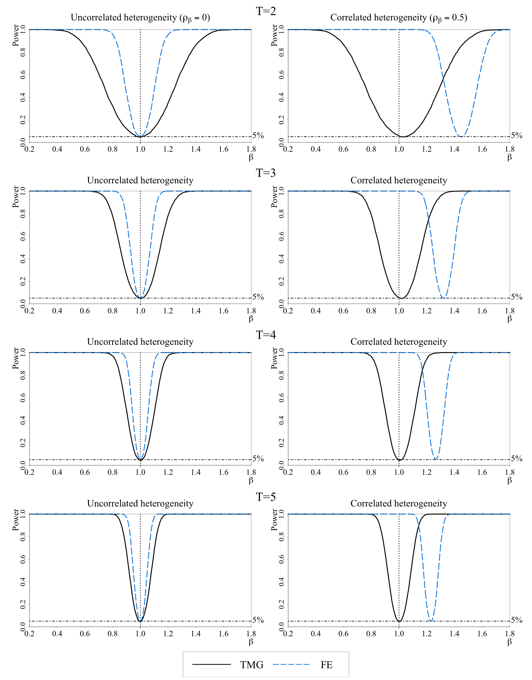
Figure 1: Empirical power functions for FE and TMG estimators of $\beta_{0}$ $(E(\beta_{i})=\beta_{0}=1)$ in the baseline model without time effects for $n=10,000$ and $T=2,3,4,5$

Notes: For details of the baseline model without time effects, see footnote (i) to Table 1. For the FE estimator, see footnote (ii) to Table 1. For the TMG estimator, see footnotes (ii) and (iii) to Table 1.

Figure 1 shows the plots of the empirical power functions for TMG and FE estimators for $n=10,000$ and $T=2,3,4$ and $5$. The left panel gives the power functions for the case of uncorrelated heterogeneity ($\rho_{\beta}=0$), and as can be seen, both estimators are centered correctly around $\beta_{0}=1$, with the FE estimator having better power properties. But the differences between the power of FE and TMG estimators shrink rapidly and become negligible as $T$ is increased from $T=2$ to $T=5$. The right panel of the figure provides the same results but under correlated heterogeneity with $\rho_{\beta}=0.5$. In this case, the empirical power functions of the FE estimator now shift dramatically to the right, away from the true value, an outcome that becomes more concentrated as $T$ is increased. In contrast, the empirical power functions for the TMG estimator tend to be reasonably robust to the choice of $\rho_{\beta}$.

To summarize, in the case of uncorrelated heterogeneity, the FE estimator performs well despite of the heterogeneity and is more efficient than the TMG estimator in the case of baseline model used in our MCs, but in general the relative efficiency of TMG and FE estimators depends on the underlying DGP. The situation is markedly different when heterogeneity is correlated, and the FE estimator can be badly biased, leading to incorrect inference, whilst the TMG estimator provides valid inference with size around the nominal five per cent level and reasonable power, irrespective of whether $\beta_{i}$ is correlated with $x_{it}$ or not.

8.2.2 Comparison of TMG, GP, and SU estimators

Focusing on the case of correlated heterogeneity, we now compare the performance of the TMG estimator with GP and SU estimators. To implement the GP estimator, defined by (3.1), for $T=2$ we follow GP and set $h_{n}=C_{GP}n^{-\alpha_{GP}}$, with $\alpha_{GP}=1/3$, and $C_{GP}=\frac{1}{2}\min\left(\hat{\sigma}_{D},\hat{r}_{D}/1.34\right)$, where $\hat{\sigma}_{D}$ and $\hat{r}_{D}$ are the respective sample standard deviation and interquartile range of $\mathop{\mathrm{d}et}(\boldsymbol{W}_{i})$. See page 2138 in Graham and Powell (2012). There is no clear guidance in GP as to the choice of $h_{n}$ when $T=3$. For consistency, for GP estimates we continue to use their bandwidth, $h_{n}=C_{GP}n^{-\alpha_{GP}}$ with $\alpha_{GP}=1/3$, but set $C_{GP}=(\bar{d}_{n})^{1/2}$ and trim if $d_{i}=\det(\mathbf{W}_{i}^{\prime}\mathbf{W}_{i})<$ $h_{n}^{2}$. The sensitivity of the results to the other choices of $\alpha_{GP}$ is considered below. For SU we use the code made available to us by the authors, which is applicable only when $T=2$.

The bias, RMSE and size for all three estimators are summarized in Table 2 for $T=2$, and $n=1,000,2,000,5,000,10,000$. For $T=3$ the results are provided for TMG and GP estimators only. The associated empirical power functions are provided in Figure 2.

Table 2: Bias, RMSE and size of TMG, GP and SU estimators of $\beta_{0}$ $(E(\beta_{i})=\beta_{0}=1)$ in the baseline model without time effects and with correlated heterogeneity, $\rho_{\beta}=0.5$

		$T=2$					$T=3$
		$\hat{\pi}$			Size		$\hat{\pi}$			Size
Estimator		$(\times 100)$	Bias	RMSE	$(\times 100)$		$(\times 100)$	Bias	RMSE	$(\times 100)$
	$n=1,000$
TMG		31.2	0.048	0.35	4.9		16.5	0.023	0.20	5.2
GP		4.2	-0.029	0.83	4.5		2.0	-0.002	0.27	4.6
SU		4.2	-0.045	1.62	4.9		…	…	…	…
	$n=2,000$
TMG		28.5	0.044	0.27	5.3		14.1	0.018	0.16	5.4
GP		3.4	0.031	0.70	5.8		1.3	0.003	0.22	4.4
SU		3.4	0.008	1.39	5.5		…	…	…	…
	$n=5,000$
TMG		24.7	0.037	0.18	4.7		10.8	0.016	0.11	5.3
GP		2.5	0.009	0.52	5.2		0.7	-0.001	0.15	5.2
SU		2.5	0.003	1.01	4.9		…	…	…	…
	$n=10,000$
TMG		22.1	0.029	0.14	5.6		8.8	0.013	0.08	5.3
GP		2.0	0.002	0.41	4.3		0.5	-0.002	0.11	4.9
SU		2.0	0.007	0.82	5.2		…	…	…	…

Notes: (i) GP and SU estimators are proposed by Graham and Powell (2012) and Sasaki and Ura (2021), respectively. The GP estimator is given by (3.1). For $T=2$, GP compare $d_{i}^{1/2}$ with the bandwidth $h_{n}=C_{GP}n^{-\alpha_{GP}}$. $\alpha_{GP}$ is set to 1/3. $C_{GP}=\frac{1}{2}\min\left(\hat{\sigma}_{D},\hat{r}_{D}/1.34\right)$, where $\hat{\sigma}_{D}$ and $\hat{r}_{D}$ are the respective sample standard deviation and interquartile range of $\mathop{\mathrm{d}et}(\boldsymbol{W}_{i})$. For $T=3$, we continue using the bandwidth $h_{n}$ with $C_{GP}=(\bar{d}_{n})^{1/2}$. See Section 8.2.2 for details. When $T=2$, the SU estimator uses the same bandwidth as GP. (ii) For details of the baseline model without time effects, see footnote (i) to Table 1. For the TMG estimator and its trimming threshold, see footnotes (ii) and (iii) to Table 1. $\hat{\pi}$ is the simulated fraction of individual estimates being trimmed, defined by (4.7). The estimation algorithm for the SU estimator is not available for $T=3$, denoted by “…”.

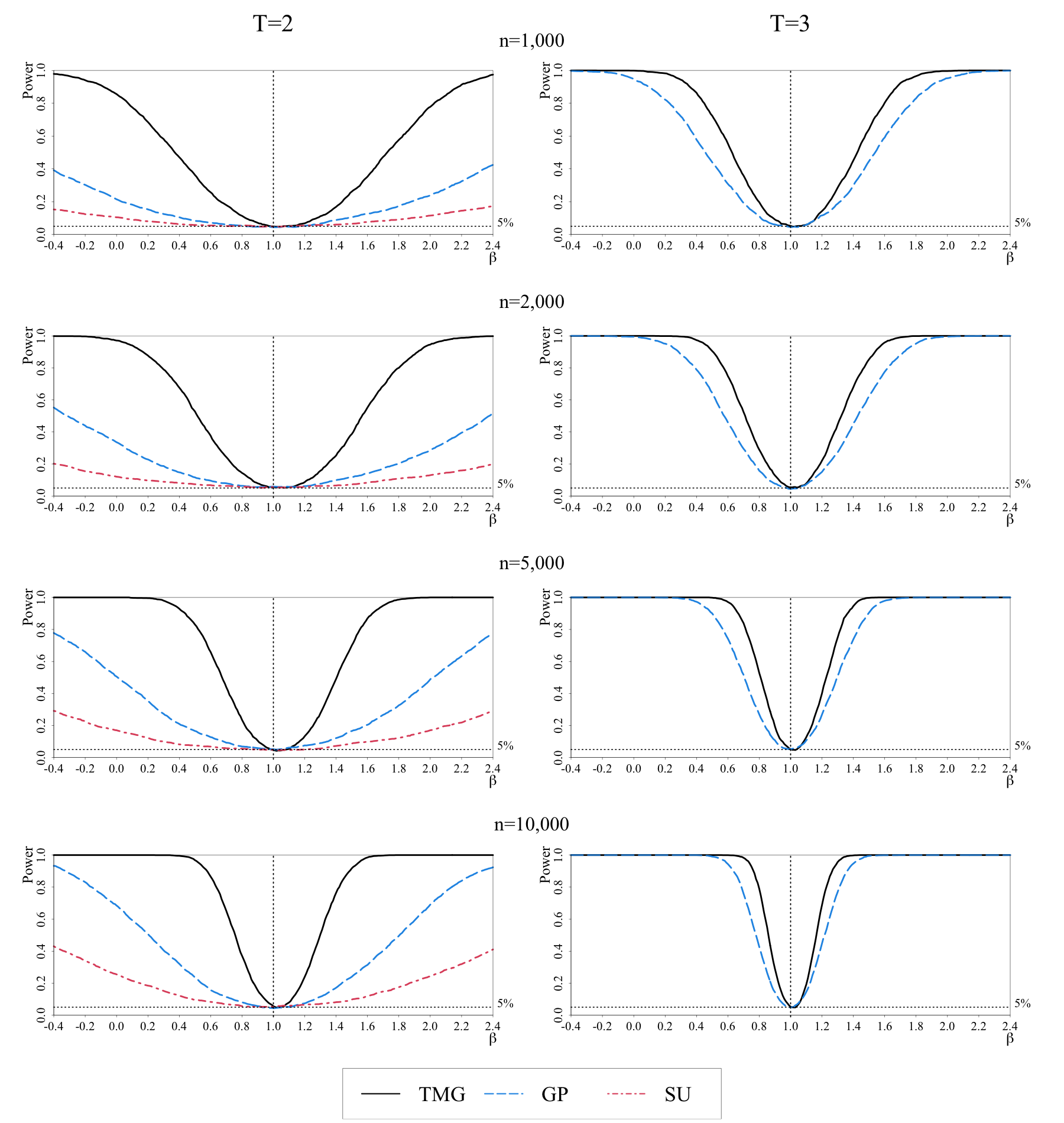
Figure 2: Empirical power functions for TMG, GP and SU estimators of $\beta_{0}$ $(E(\beta_{i})=\beta_{0}=1)$ in the baseline model without time effects and with correlated heterogeneity, $\rho_{\beta}=0.5$, for $n=1,000,\,2,000,\,5,000,\,10,000$ and $T=2,3$

Notes: For details of the baseline model without time effects, see footnote (i) to Table 1. For the TMG estimator, see footnote (ii) to Table 1. For GP and SU estimators, see footnote (i) to Table 2.

The fraction of the trimmed estimates, $\pi_{n}$, defined by (4.7), for the TMG estimator is quite high when $T=2$, but declines markedly when $T$ is raised to $3,$ and to a lesser extent as $n$ is increased. This is not the case for the other two estimators. For example, when $T=2$ and $n=1,000$, the fraction of trimmed estimates for the TMG estimator is around $31.2$ per cent as compared to $4.2$ per cent for GP and SU estimators, and falls to $22.1$ per cent as $n$ is increased to $10,000$. Increasing $T$ from $2$ to $3$ with $n=1,000$ reduces this fraction to $16.5$ per cent as compared to $2$ per cent for the GP estimator. The heavy trimming causes the TMG estimator to have a much larger bias than GP and SU estimators, particularly when $T=2$ and $n$ is sufficiently large. However, the TMG estimator continues to have better overall small sample performance due to its higher efficiency. Recall that the TMG estimator makes use of the trimmed estimates, as set out in the second term of (4.6), but the trimmed estimates are not used in the GP estimator. This difference in the way trimmed estimates are treated is reflected in the lower RMSE of the TMG estimator as compared to the other two estimators for all $T$ and $n$ combinations. For example, when $T=2$ and $n=1,000$, the RMSE of the TMG is $0.35$ as compared to $0.83$ and $1.62$ for GP and SU estimators. The relative advantage of the TMG estimator continues when $T$ is increased from $2$ to $3$, but its relative advantage declines. For $T=3$, the RMSE of the TMG estimator stands at $0.20$ compared to $0.27$ for the GP estimator. The larger the value of $T$, the less important the trimming becomes.

The empirical power functions for all three estimators are shown in Figure 2. As can be seen, the TMG estimator is uniformly more powerful than the GP estimator and the GP estimator is more powerful than the SU estimator.

8.2.3 Models with time effects

Adding time effects to the panel regressions does not alter the above conclusions. The MC results for estimation of $\beta_{0}$ and the time effects $\boldsymbol{\phi}=(\phi_{1},\phi_{2})^{\prime}$ are summarized in Tables 3 and 4, respectively. The small sample properties of the TMG-TE estimator of $\beta_{0}$ are very close to those reported for the TMG estimator in Table 2. Interestingly, there are also little differences between TMG-TE and TMG-C estimators of $\beta_{0}$ when $T=3$, as can be seen from the right panel of Table 3. Also, the time effects are precisely estimated. Bias, RMSE and size for TMG-TE and GP estimators of $\boldsymbol{\phi}=(\phi_{1},\phi_{2})^{\prime}$ are summarized in Table 4. The bias of TMG-TE and GP estimators of $\phi_{1}$ are similar, but the TMG-TE estimator has much lower RMSEs and higher power when $T=2$. A comparison of the empirical powers of these two estimators is given in Figures S.9–S.11 in the online supplement.

Table 3: Bias, RMSE and size of TMG-TE, TMG-C, GP and SU estimators of $\beta_{0}$ $(E(\beta_{i})=\beta_{0}=1)$ in the baseline model with time effects and correlated heterogeneity, $\rho_{\beta}=0.5$

		$T=2$					$T=3$
		$\hat{\pi}$			Size		$\hat{\pi}$			Size
Estimator		$(\times 100)$	Bias	RMSE	$(\times 100)$		$(\times 100)$	Bias	RMSE	$(\times 100)$
	$n=1,000$
TMG-TE		31.2	0.048	0.35	5.0		16.5	0.023	0.20	5.4
TMG-C		…	…	…	…		16.5	0.023	0.20	5.2
GP		4.2	-0.034	0.84	3.9		2.0	-0.002	0.27	4.6
SU		4.2	-0.052	1.67	5.3		…	…	…	…
	$n=2,000$
TMG-TE		28.5	0.044	0.27	5.6		14.1	0.018	0.16	5.5
TMG-C		…	…	…	…		14.1	0.018	0.16	5.6
GP		3.4	0.032	0.71	5.2		1.3	0.003	0.22	4.6
SU		3.4	0.012	1.40	5.8		…	…	…	…
	$n=5,000$
TMG-TE		24.7	0.037	0.18	4.7		10.8	0.016	0.11	5.3
TMG-C		…	…	…	…		10.8	0.016	0.11	5.3
GP		2.5	0.008	0.53	5.0		0.7	-0.001	0.15	5.1
SU		2.5	0.006	1.02	4.7		…	…	…	…
	$n=10,000$
TMG-TE		22.1	0.028	0.14	5.7		8.8	0.013	0.08	5.3
TMG-C		…	…	…	…		8.8	0.013	0.08	5.3
GP		2.0	0.003	0.41	4.4		0.5	-0.002	0.11	5.0
SU		2.0	0.011	0.82	5.5		…	…	…	…

Notes: (i) The baseline model is generated as $y_{it}=\alpha_{i}+\phi_{t}+\beta_{i}x_{it}+u_{it}$, with time effects given by $\phi_{t}=t$ for $t=1,2,...,T-1$, and $\phi_{T}=-T(T-1)/2$. The errors processes for $y_{it}$ and $x_{it}$ equations are chi-squared and Gaussian, respectively, $x_{it}$ are generated as heterogeneous AR(1) processes, and $\rho_{\beta}$ (the degree of correlated heterogeneity) is defined by (8.6). For further details see Section 8.1.3. (ii) The TMG-TE estimators of $\boldsymbol{\theta}_{0}$ and $\boldsymbol{\phi}$ are given by (6.9) and (6.11), respectively, and their asymptotic variances are estimated by (A.3.4) and (A.3.7), respectively, in the Appendix. The TMG-C estimators of $\boldsymbol{\theta}_{0}$ and $\boldsymbol{\phi}$ are given by (6.20) and (6.17), respectively, and their asymptotic variances are estimated by (6.21) and (6.19), respectively. For the trimming threshold, see footnote (iii) to Table 1. (iii) For GP and SU estimators, see footnote (i) to Table 2. $\hat{\pi}$ is the simulated fraction of individual estimates being trimmed, defined by (4.7). “…” denotes the estimation algorithms are not available or not applicable.

Table 4: Bias, RMSE and size of TMG-TE and GP estimators of the time effects, $\phi_{1}$ and $\phi_{2}$, in the baseline model with correlated heterogeneity, $\rho_{\beta}=0.5$

				$n=1,000$				$n=5,000$
		Estimator		Bias	RMSE	Size $(\times 100)$		Bias	RMSE	Size $(\times 100)$
					$T=2$				$T=2$
$\phi_{1}=1$		TMG-TE		0.002	0.09	6.1		-0.001	0.04	4.8
		GP		0.001	0.54	7.1		-0.008	0.35	6.9
					$T=3$				$T=3$
$\phi_{1}=1$		TMG-TE		-0.002	0.10	5.6		0.001	0.05	4.9
		GP		0.004	0.15	5.7		0.001	0.07	5.0
$\phi_{2}=2$		TMG-TE		-0.006	0.10	5.7		0.000	0.05	4.9
		GP		-0.010	0.13	5.3		0.000	0.06	4.2

Notes: For the baseline model with time effects, see footnote (i) to Table 3. For the TMG-TE estimator, see footnote (ii) to Table 3. For the GP estimator, see footnote (i) to Table 2.

8.2.4 Sensitivity of TMG and GP estimators to the choice of the threshold values

Finally, we consider the sensitivity of TMG and GP estimators to the choice of threshold values. The baseline value of the threshold value for the GP estimator, $\alpha_{GP}=1/3$ as recommended by GP. But for the purpose of comparison with the TMG estimator computed for $\alpha=1/3,0.35$ and $1/2$, we also consider $\alpha_{GP}=0.35/2$ and $1/4$. Recall that the bandwidth, $h_{n}^{2}$, used by GP corresponds to $a_{n}$ used in the specification of TMG. Hence, $2\alpha_{GP}$ corresponds to $\alpha$. For comparability, we decided to consider values of $\alpha_{GP}$ below $1/3$ required by GP’s theory. This allows us to compare GP and TMG focusing on the utility of including both trimmed and untrimmed estimates of $\mathbf{\theta}_{i}$ in estimation of average treatment effects.

The results are summarized in Section S.4.2 of the online supplement. As can be seen from Table S.5 there is a clear trade-off between bias and variance as $\alpha$ and $\alpha_{GP}$ are increased. For $T=2$, the TMG estimator is biased when $\alpha=1/3$ (as predicted by the theory), but has a lower variance with its RMSE declining as $\alpha$ is increased from $1/3$ to $1/2$. This trade-off is less consequential when $T$ is increased to $T=3$. The same is also true for the GP estimator. But for all choices of $\alpha$ and $\alpha_{GP}$ the TMG performs better in terms of RMSE when $T=2$. For $T=3$, TMG and GP estimators share the same trimming threshold when $\alpha=2\alpha_{GP}$, resulting in identical trimmed fractions for $\alpha=2\alpha_{GP}\in\{0.35,1/2\}$. While RMSEs are similar, the GP estimator exhibits significantly higher bias than the TMG estimator as observations of the trimmed units are not exploited by the GP estimator.

Figure S.2 compares power functions of TMG and GP estimators with $\alpha=2\alpha_{GP}=0.35$. For $T=2$, a higher trimmed fraction results in a steeper power function for the TMG estimator as compared to that of the GP estimator. When $T=3$, with the same trimmed fraction, the power function of the GP estimator shifts to the right, away from the true value. The substantial differences in power performance of the TMG estimator with $\alpha=1/3$ and the GP estimator with $\alpha_{GP}=1/3$ are also illustrated in Figure S.3.

The power comparisons of TMG and GP estimators for different values of $\alpha$ and $\alpha_{GP}$ are given in Figures S.4 and S.5, respectively, and convey the same message, suggesting that for the TMG estimator the boundary choice of $\alpha=1/3$ tends to produce the best bias-variance trade-off. Increasing $\alpha$ reduces the bias but increases the variance, and the boundary value derived theoretically seems to strike a sensible balance and is recommended.

8.2.5 MC evidence on the Hausman-type test of correlated heterogeneity

Table 5: Empirical size and power of the Hausman-type test of correlated heterogeneity in the baseline model without time effects

		Under $H_{0}$										Under $H_{1}$
		Homogeneity: $\sigma_{\beta}^{2}=0$					Uncorrelated hetro.: $\rho_{\beta}=0$, $\sigma_{\beta}^{2}=0.5$					Correlated hetro.: $\rho_{\beta}=0.5$, $\sigma_{\beta}^{2}=0.5$
$T/n$		1,000	2,000	5,000	10,000		1,000	2,000	5,000	10,000		1,000	2,000	5,000	10,000
2		4.1	4.4	5.3	5.5		5.6	5.5	4.8	5.9		26.0	39.0	69.8	90.8
3		4.5	5.7	5.8	4.8		5.3	4.5	5.7	4.7		41.0	61.5	91.3	99.6
4		4.9	5.7	5.6	4.9		4.8	4.5	5.5	4.7		53.5	77.2	97.8	100.0
5		5.3	4.6	4.9	5.2		4.3	4.6	4.4	4.3		63.5	86.1	99.5	100.0
6		4.8	5.2	5.5	5.3		5.2	4.4	4.6	4.4		72.0	91.7	100.0	100.0
8		5.0	4.8	5.0	5.3		4.6	4.9	6.0	5.7		81.1	96.2	100.0	100.0

Notes: (i) The baseline model for the Hausman-type test is generated as $y_{it}=\alpha_{i}+\beta_{i}x_{it}+u_{it}$, with $\alpha_{i}$ correlated with $x_{it}$ under both the null and alternative hypotheses. The errors processes for $y_{it}$ and $x_{it}$ equations are chi-squared and Gaussian, respectively, and $x_{it}$ are generated as heterogeneous AR(1) processes. For further details see Section 8.1.3. (ii) The null hypothesis is given by (7.1), including the case of homoegenity with $\sigma_{\beta}^{2}=0$ and the case of uncorrelated heterogeneity with $\rho_{\beta}=0$ (the degree of correlated heterogeneity defined by (8.6) and $\sigma_{\beta}^{2}=0.5$. The alternative of correlated heterogeneity is generated with $\rho_{\beta}=0.5$ and $\sigma_{\beta}^{2}=0.5$. (iii) The test statistic is calculated based on the difference between FE and TMG estimators, given by (7.3). Under $H_{0}$, the test statistic is asymptotically distributed as $\chi_{k-1}^{2}$ as $n\rightarrow\infty$. For the FE estimator, see footnote (ii) to Table 1. For the TMG estimator, see footnotes (ii) and (iii) to Table 1. Size and power are in per cent.

Table 5 reports empirical size and power of the Hausman-type test of correlated heterogeneity given by (7.3). The left, middle and right panels report the results under homogeneity, uncorrelated heterogeneity and correlated heterogeneity in slope coefficients. In the left and middle panels, the size of the test is around the nominal level of 5 per cent. As shown in the paper, when $\boldsymbol{x}_{it}$ is strictly exogenous and $\boldsymbol{\beta}_{i}$ is mean independent of $\boldsymbol{X}_{i}$, FE, MG and TMG estimators are all consistent under homogeneity and uncorrelated heterogeneity, and in this case the Hausman-type test does not have power against uncorrelated heterogeneity. However, in the case where slope coefficients are heterogeneous and correlated with the regressors, the MG and TMG estimators are consistent when they have at least finite second moments, while the FE estimator is biased for all $T$. In this case, we would expect the proposed test to have power, and this is indeed evident in the right panel of Table 5. Also the power of the test rises with increases in $n$ even when $T=2$, illustrating the (ultra) small $T$ consistency of the proposed test.

The MC evidence on the performance of our proposed test of correlated heterogeneity in the case of panels with time effects is given in Table S.15 of the online supplement. We consider two versions of the test, depending on how time effects are filtered out, namely TMG-TE and TMG-C estimators (see equations (S.2.15) and (S.2.21)). The empirical size and power of these two test statistics are comparable for $T>2$. More importantly, allowing for time effects has negligible effects on the small sample performance of the test, while the power of the test is slightly lower than the power reported in Table 5 for models without time effects. Increases in $n$ and/or $T$ result in a rapid rise in power, illustrating the consistent property of the proposed test.

9 Empirical illustration

In this section, we re-visit the empirical application in Graham and Powell (2012) who provide estimates of the average effect of household expenditures on calorie demand, based on a sample of households from poor rural communities in Nicaragua that participated in a conditional cash transfer program Red de Proteccion Social (RPS). The data set is a balanced panel with $n=1,358$ households observed from 2000 to 2002. We present estimates of the average treatment effects using the following panel data model with time effects:

$$\ln(Cal_{it})=\alpha_{i}+\phi_{t}+\beta_{i}\ln(Exp_{it})+u_{it},$$ (9.1)

where $\ln(Cal_{it})$ denotes the logarithm of household calorie availability per capita in year $t$ of household $i$, and $\ln(Exp_{it})$ denotes the logarithm of real household expenditures per capita (in thousands of 2001 cordobas) of household $i$ in year $t$. The parameter of interest is the average treatment effect defined by $\beta_{0}=E(\beta_{i})$, allowing for possible dependence between $\beta_{i}$ and $\ln(Exp_{it})$. Correlated heterogeneity could arise for a number of reasons, such as model misspecification, individuals responding strategically to treatments, and common factors that simultaneously affect $\beta_{i}$ and the treatment, $\ln(Exp_{it})$. It is, therefore, prudent to first test for correlated heterogeneity before estimating $\beta_{0}$ by fixed effects, which is the standard approach when $T$ is ultra short. We provide test statistics and estimates of $\beta_{0}$ for the panels of 2001–2002 $(T=2)$ and 2000–2002 $(T=3)$ with and without time effects.

Table 6 reports results of the Hausman-type test of correlated heterogeneity in the effects of household expenditures on calorie demand. The null hypothesis is rejected for both panels covering the periods 2001–2002 and 2000–2002, and irrespective of whether time effects are allowed. As shown in the Monte Carlo experiments, the test only has power against the alternative of correlated heterogeneity. Therefore, these results provide strong evidence of heterogeneity in the treatment effects that are correlated with the level of household expenditures, which in turn sheds doubt on the validity of the FE estimation of the average treatment effect for this application.

Table 6: Hausman-type statistics for testing correlated heterogeneity in the effects of household expenditures on calorie demand in Nicaragua

	Without time effects				With time effects
	2001–2002		2000–2002		2001–2002		2000–2002
					TMG-TE		TMG-TE	TMG-C
Statistics	5.918		7.626		5.959		6.772	7.653
$p$-value	0.015		0.006		0.015		0.009	0.006
$T$	2		3		2		3	3

Notes: The test is applied to the average effect $\beta_{0}=E(\beta_{i})$ in the model (9.1) based on the RPS panel of $1,358$ households. The test statistic for panels without time effects is described in footnote (iii) to Table 5. The test statistics for panels with time effects are based on the difference between the FE-TE and TMG-TE estimators given by (S.2.15) with $T\geq 2$, and the difference between the FE-TE and TMG-C estimators given by (S.2.21) with $T>2$. For further details see Section S.2 in the online supplement.

Table 7: Alternative estimates of the average effect of household expenditures on calorie demand in Nicaragua over the period 2001–2002 ($T=2$)

	Without time effects					With time effects
	(1)	(2)	(3)	(4)		(5)	(6)	(7)	(8)
	FE	GP	SU	TMG		FE-TE	GP	SU	TMG-TE
$\hat{\beta}_{0}$	0.6568	0.4549	0.6974	0.5623		0.6554	0.4629	0.6952	0.5612
	(0.0287)	(0.1003)	(0.1689)	(0.0425)		(0.0284)	(0.1025)	(0.1650)	(0.0424)
$\hat{\phi}_{2002}$	…	…	…	…		0.0172	-0.0181	…	0.0178
	…	…	…	…		(0.0063)	(0.0296)	…	(0.0064)
$\hat{\pi}$ $(\times 100)$	…	3.8	3.8	27.1		…	3.8	3.8	27.1

Notes: The estimates of $\beta_{0}=E(\beta_{i})$ and $\phi_{2002}$ in the model (9.1) are based on the RPS panel of $1,358$ households. The FE estimator is described in the footnote (ii) to Table 1. GP and SU estimators are described in footnote (i) to Table 2. The TMG estimator is described in footnotes (ii) and (iii) to Table 1. The FE-TE estimator is the two-way fixed effects estimator given by (S.2.1) in the online supplement. TMG-TE and TMG-C estimators are described in footnote (ii) to Table 3. $\hat{\pi}$ is the estimated fraction of individual estimates being trimmed, defined by (4.7). The numbers in brackets are standard errors. “…” denotes the estimation algorithms are not available or not applicable.

Table 7 presents the estimates of $\beta_{0}$ based on the panel of 2001–2002 (with $T=2$) without time effects (left panel), and with time effects (right panel). The estimates are not affected by the inclusion of time effects but differ considerably across different methods. Based on the test results reported in Table 6, the FE estimates are most likely biased. Turning to the trimmed estimators, we find that only the TMG estimator is heavily trimmed with 27.1 per cent of the estimates being trimmed, whilst the rate of trimming is only around 3.8 per cent for GP and SU estimators. Focussing on the estimates without time effects, we find the FE estimate, 0.6568 (0.0287), is much larger and more precisely estimated than either the GP or TMG estimates, given by 0.4549 (0.1003) and 0.5623 (0.0425), respectively. Judging by the standard errors, it is also noticeable that the TMG is more precisely estimated than the GP estimate and lies somewhere between the FE and GP estimates. In contrast, the SU estimate of 0.6974 (0.1689) is close to the FE estimate but with a much larger degree of uncertainty. These estimates are in line with the MC results reported in the previous section, where we found that in the presence of correlated heterogeneity FE estimates are biased with smaller standard errors (thus leading to incorrect inference), whilst GP and TMG estimators are correctly centered with the TMG estimator being more efficient.

Table 8: Alternative estimates of the average effect of household expenditures on calorie demand in Nicaragua over the period 2000–2002 ($T=3$)

	Without time effects				With time effects
	(1)	(2)	(3)		(4)	(5)	(6)	(7)
	FE	GP	TMG		FE-TE	GP	TMG-TE	TMG-C
$\hat{\beta}_{0}$	0.6588	0.6034	0.5900		0.6968	0.6448	0.6370	0.6338
	(0.0233)	(0.0350)	(0.0284)		(0.0211)	(0.0330)	(0.0263)	(0.0261)
$\hat{\phi}_{2001}$	…	…	…		0.0727	0.0682	0.0708	0.0682
	…	…	…		(0.0087)	(0.0123)	(0.0088)	(0.0123)
$\hat{\phi}_{2002}$	…	…	…		0.1066	0.0954	0.1054	0.0682
	…	…	…		(0.0080)	(0.0108)	(0.0080)	(0.0123)
$\hat{\pi}$ $(\times 100)$	…	1.2	10.9		…	1.2	10.9	10.9

Notes: The estimates of $\beta_{0}=E(\beta_{i})$ and $(\phi_{2001},\phi_{2002})^{\prime}$ in the model (9.1) are based on the RPS panel of $1,358$ households. $\hat{\pi}$ is the estimated fraction of individual estimates being trimmed, defined by (4.7). See also footnotes to Table 7.

Table 8 gives the estimates of $\beta_{0}$ for the extended panel, 2000–2002 (with $T=3$), both with and without time effects. When time effects are included we provide two versions of the TMG estimates (TMG-TE and TMG-C), depending on how time effects are estimated. As in the case of the 2001–2002 panel, the FE estimates are larger than the GP and TMG estimates, but these differences are reduced somewhat, particularly when time effects are included in the panel regressions. Further, as expected, increasing $T$ reduces the rate of trimming and brings the GP and TMG estimators closer to one another. The trimming rate for the GP estimator is very small indeed (only 1.2 per cent), as compared to around 11 per cent for the TMG estimator in the case of the 2000–2002 panel. The TMG-TE and TMG-C estimates of the time effects ($\phi_{2001}$ and $\phi_{2002}$) are quite close and are both highly statistically significant and positive, capturing the upward trend in the calorie intake.

10 Conclusions

This paper studies estimation of average treatment effects in panel data models with possibly correlated heterogeneous coefficients, when the number of cross-sectional units is large, but the number of time periods can be as small as the number of regressors. We recall that the FE estimator is inconsistent under correlated heterogeneity, and the MG estimator can have unbounded first or second moments when applied to ultra short panels. Thus, the TMG estimator is proposed, where the trimming process is derived by a careful examination of the bias/efficiency trade-off in the asymptotic distribution. Conditions under which the TMG estimator is consistent and asymptotically normally distributed are provided. We also propose new estimators for ultra short panel data models with time effects, distinguishing between cases where $T>$ $k$ and $T\geq k$, and derive their asymptotic distributions under the identifying condition that the dependence between heterogeneous slope coefficients and the regressors is time-invariant. Moreover, based on differences between the TMG and FE estimators (without and with time effects), we propose Hausman-type tests of correlated slope heterogeneity which must be applied before using FE or FE-TE estimators in practice.

Using Monte Carlo experiments, we highlight the bias and size distortion properties of the FE and FE-TE estimators under correlated heterogeneity. In contrast, the TMG and TMG-TE estimators are shown to have desirable finite sample performance under a number of different MC designs, allowing for Gaussian and non-Gaussian heteroskedastic error processes, dynamic heterogeneity and interactive time effects in the covariates, and different choices of the trimming threshold parameter, $\alpha$. In particular, since the TMG and TMG-TE estimators exploit information on untrimmed and trimmed estimates alike, they have the smallest RMSE, and tests based on them have the correct size and are more powerful compared with the other trimmed estimators currently proposed in the literature.

The Hausman-type tests based on TMG and TMG-TE estimators are also shown to have very good small sample properties, with their size controlled and their power rising strongly with $n$ even when $T=k=2$. It is hoped that the new Hausman test provides empirical investigators with a diagnostic test that can be used before the application of the FE-TE estimators that are commonly used in the empirical literature. It is hoped that the use of this diagnostic test can help researchers in avoiding biased estimates and possibly misleading inferences. When the TMG and TMG-TE estimators and the Hausman-type tests of correlated heterogeneity are applied to a panel of households in poor rural communities in Nicaragua, the results provide clear evidence of correlated heterogeneity in the average effect of household expenditures on calorie demand, which sheds doubt on the application of FE-TE estimators to this data set.

Finally, we would like to end by acknowledging that, similarly to the FE-TE estimators, the validity of the TMG-TE and TMG-C estimators requires the so-called parallel trends assumption where time effects are assumed to have homogeneous effects across all individual units in the panel. Relaxing the parallel trends assumption in short $T$ panels has been an important area of active research, but most of these contributions either assume homogeneous slopes or restricted forms of slope heterogeneity, or place restrictions on the time effects. The development of techniques for estimation and inference in ultra short panels with correlated heterogeneous slopes and interactive effects is a topic for future research.

Appendix

Notations: Generic positive finite constants are denoted by $C$ when large, and $c$ when small. They can take different values at different instances. $\lambda_{\max}\left(\boldsymbol{A}\right)$ and $\lambda_{\min}\left(\boldsymbol{A}\right)$ denote the maximum and minimum eigenvalues of matrix $\boldsymbol{A}$. $\boldsymbol{A}\succ\boldsymbol{0}$ and $\boldsymbol{A}\succeq\boldsymbol{0}$ denote that $\boldsymbol{A}$ is a positive definite and a non-negative definite matrix, respectively. $\left\|\boldsymbol{A}\right\|=\lambda_{\max}^{1/2}(\boldsymbol{A}^{\prime}\boldsymbol{A)}$ and $\left\|\boldsymbol{A}\right\|_{1}$ denote the spectral and column norms of matrix $\boldsymbol{A}$, respectively. $\boldsymbol{A}^{\ast}$ denotes the adjoint of $\boldsymbol{A},$ such that $\boldsymbol{A}^{-1}=d^{-1}\boldsymbol{A}^{\ast}$, and $d=det(\boldsymbol{A)}$. $\left\|\boldsymbol{x}\right\|_{p}=\left[E\left(\left\|\boldsymbol{x}\right\|^{p}\right)\right]^{1/p}$. If $\left\{f_{n}\right\}_{n=1}^{\infty}$ is any real sequence and $\left\{g_{n}\right\}_{n=1}^{\infty}$ is a sequences of positive real numbers, then $f_{n}=O(g_{n})$, if there exists $C$ such that $\left|f_{n}\right|/g_{n}\leq C$ for all $n$. $f_{n}=o(g_{n})$ if $f_{n}/g_{n}\rightarrow 0$ as $n\rightarrow\infty$. Similarly, $f_{n}=O_{p}(g_{n})$ if $f_{n}/g_{n}$ is stochastically bounded, and $f_{n}=o_{p}(g_{n}),$ if $f_{n}/g_{n}\rightarrow_{p}0$. The operator $\rightarrow_{p}$ denotes convergence in probability, and $\rightarrow_{d}$ denotes convergence in distribution.

Appendix A.1 Lemmas

Lemma A.1

Suppose that Assumptions 2, 5 and 6 hold. Then for each $i$, we have

$$E\left[d_{i}^{s}\boldsymbol{1}\{d_{i}\leq a_{n}\}\right] =O(a_{n}^{s+1})\text{, for }s=1,2,...,$$ (A.1.1)

$$E(\delta_{i}) =O(a_{n}),\text{ and }E(\delta_{i}^{2})=O(a_{n}),$$ (A.1.2)

$$E\left(\delta_{i}\boldsymbol{\eta}_{i}\right) =O(a_{n}),\text{ and }E\left(\delta_{i}^{2}\boldsymbol{\eta}_{i}\right)=O(a_{n}),$$ (A.1.3)

$$n^{-1}\sum_{i=1}^{n}\left\{E\left[d_{i}^{2}\boldsymbol{1}\{d_{i}\leq a_{n}\}\right]\right\}^{1/2} =O(a_{n}^{3/2}),$$ (A.1.4)

$$n^{-1}\sum_{i=1}^{n}\left\{E\left[d_{i}^{-2}\boldsymbol{1}\{d_{i}>a_{n}\}\right]\right\}^{1/2} =O(a_{n}^{-1}).$$ (A.1.5)

Proof. By mean value theorem (MVT), under Assumption 5, we have

$$F_{d}(a_{n})=F_{d}(0)+f_{d}(\bar{a}_{n})a_{n}=f_{d}(\bar{a}_{n})a_{n}=O(a_{n}),$$ (A.1.6)

where $\bar{a}_{n}$ lies on the line segment between $0$ and $a_{n}$. Similarly, let $\psi(a_{n})=\int_{0}^{a_{n}}u^{s}f_{d}(u)du$ and note that $\psi^{\prime}(a_{n})=a_{n}^{s}f_{d}(a_{n})$. Then by MVT $\psi(a_{n})=\psi(0)+\left[\bar{a}_{n}^{s}f_{d}(\bar{a}_{n})\right]a_{n}$, and we have

$$E\left[d_{i}^{s}\boldsymbol{1}\{d_{i}\leq a_{n}\}\right]=\int_{0}^{a_{n}}u^{s}f_{d}(u)du=\bar{a}_{n}^{s}f_{d}(\bar{a}_{n})a_{n}=O(a_{n}^{s+1})\text{, for }s=1,2,....$$ (A.1.7)

Using the above results

$$E(\delta_{i})= E\left[\left(\frac{d_{i}-a_{n}}{a_{n}}\right)\boldsymbol{1}\{d_{i}\leq a_{n}\}\right]=a_{n}^{-1}E\left[d_{i}\boldsymbol{1}\{d_{i}\leq a_{n}\}\right]-E\left[\boldsymbol{1}\{d_{i}\leq a_{n}\}\right]$$

$$= a_{n}^{-1}O(a_{n}^{2})-F_{d}(a_{n})=O(a_{n}),$$ (A.1.8)

and

$$E(\delta_{i}^{2}) =E\left[\left(\frac{d_{i}-a_{n}}{a_{n}}\right)^{2}\boldsymbol{1}\{d_{i}\leq a_{n}\}\right]$$

$$=a_{n}^{-2}E\left[d_{i}^{2}\boldsymbol{1}\{d_{i}\leq a_{n}\}\right]+E\left[\boldsymbol{1}\{d_{i}\leq a_{n}\}\right]-2a_{n}^{-1}E\left[d_{i}\boldsymbol{1}\{d_{i}\leq a_{n}\}\right]$$

$$=a_{n}^{-2}O(a_{n}^{3})+F_{d}(a_{n})-2a_{n}^{-1}O(a_{n}^{2})=O(a_{n}).$$ (A.1.9)

Consider now the terms involving the products of $\delta_{i}$ and $\boldsymbol{\eta}_{i}$

$$E\left(\delta_{i}\boldsymbol{\eta}_{i}\right)=\boldsymbol{B}_{i}E\left[\left(\frac{d_{i}-a_{n}}{a_{n}}\right)\boldsymbol{1}\{d_{i}\leq a_{n}\}\left[\boldsymbol{g}(d_{i})-E\left[\boldsymbol{g}(d_{i})\right]\right]\right].$$ (A.1.10)

Since $\boldsymbol{B}_{i}$ is bounded and does not depend on $d_{i}$, without loss of generality we set $\boldsymbol{B}_{i}=\boldsymbol{I}_{k}$ and consider the the $j^{th}$ term of (A.1.10), namely

$$s_{j}(a_{n})= E\left\{\left(\frac{d_{i}-a_{n}}{a_{n}}\right)\boldsymbol{1}\{d_{i}\leq a_{n}\}\left[g_{j}(d_{i})-E\left[g_{j}(d_{i})\right]\right]\right\}$$

$$= \frac{1}{a_{n}}\int_{0}^{a_{n}}ug_{j}(u)f_{d}(u)du-\int_{0}^{a_{n}}g_{j}(u)f_{d}(u)du$$

$$-E\left[g_{j}(d_{i})\right]\left[\frac{1}{a_{n}}\int_{0}^{a_{n}}uf_{d}(u)du\right]+E\left[g_{j}(d_{i})\right]\left[\int_{0}^{a_{n}}f_{d}(u)du\right].$$

By Assumption 6 $E\left[g_{j}(d_{i})\right]<C$, and using (A.1.6) and (A.1.1) we have

$$\int_{0}^{a_{n}}f_{d}(u)du=O(a_{n})\text{, and }a_{n}^{-1}\int_{0}^{a_{n}}uf_{d}(u)du=O(a_{n}).$$

Also by the mean value theorem

$$\int_{u=0}^{a_{n}}g_{j}(u)f_{d}(u)du =g_{j}(\bar{a}_{n})f_{d}(\bar{a}_{n})a_{n}=O(a_{n}),$$

$$\frac{1}{a_{n}}\int_{u=0}^{a_{n}}ug_{j}(u)f_{d}(u)du =\frac{1}{a_{n}}\left[\bar{a}_{n}g_{j}(\bar{a}_{n})f_{d}(\bar{a}_{n})a_{n}\right]=O(a_{n}).$$

Hence, $E\left(\delta_{i}\boldsymbol{\eta}_{i}\right)=O(a_{n})$. Similarly the $j^{th}$ term of $E\left(\delta_{i}^{2}\boldsymbol{\eta}_{i}\right)$ (setting $\boldsymbol{B}_{i}=\boldsymbol{I}_{k}$) is given by

$$s_{j2}(a_{n}) = E\left\{\left(\frac{d_{i}-a_{n}}{a_{n}}\right)^{2}\boldsymbol{1}\{d_{i}\leq a_{n}\}\left[g_{j}(d_{i})-E\left[g_{j}(d_{i})\right]\right]\right\}$$ (A.1.11)

$$= E\left\{\left(\frac{d_{i}^{2}}{a_{n}^{2}}-1-2\frac{d_{i}-a_{n}}{a_{n}}\right)\boldsymbol{1}\{d_{i}\leq a_{n}\}\left[g_{j}(d_{i})-E\left[g_{j}(d_{i})\right]\right]\right\}.$$

Consider the first term

$$E\left\{\frac{d_{i}^{2}}{a_{n}^{2}}\boldsymbol{1}\{d_{i}\leq a_{n}\}\left[g_{j}(d_{i})-E\left[g_{j}(d_{i})\right]\right]\right\}$$

$$= \frac{1}{a_{n}^{2}}\int_{0}^{a_{n}}u^{2}g_{j}(u)f_{d}(u)du-\frac{1}{a_{n}^{2}}E\left[g_{j}(d_{i})\right]E\left[d_{i}^{2}\boldsymbol{1}\{d_{i}\leq a_{n}\}\right],$$

and again by mean value theorem $a_{n}^{-2}\int_{0}^{a_{n}}u^{2}g_{j}(u)f_{d}(u)du=O(a_{n})$, $E\left[g_{j}(d_{i})\right]<C$, and using (A.1.7)$\,\ E\left[d_{i}^{2}\boldsymbol{1}\{d_{i}\leq a_{n}\}\right]=O(a_{n}^{3}).$ Hence, the first term of (A.1.11) is $O(a_{n})$. For its second term, we have

$$E\left\{\boldsymbol{1}\{d_{i}\leq a_{n}\}\left[g_{j}(d_{i})-E\left[g_{j}(d_{i})\right]\right]\right\}=\int_{0}^{a_{n}}g_{j}(u)f_{d}(u)du-E\left[g_{j}(d_{i})\right]\int_{0}^{a_{n}}f_{d}(u)du=O(a_{n}),$$

and the order of the third term is already established to be $O(a_{n})$. Hence, it follows that $E\left(\delta_{i}^{2}\boldsymbol{\eta}_{i}\right)=O(a_{n})$. Finally, result (A.1.4) follows from (A.1.1) and (A.1.5) follows noting that $d_{i}^{-2}\boldsymbol{1}\{d_{i}>a_{n}\}\leq a_{n}^{-2}$.   

Lemma A.2

Suppose that Assumptions 1, 2, 4, 5 and 6, hold. Let

$$\boldsymbol{\bar{\xi}}_{\delta,nT}=n^{-1}\sum_{i=1}^{n}\left(1+\delta_{i}\right)\boldsymbol{\xi}_{iT},$$

where $\delta_{i}=\left(\frac{d_{i}-a_{n}}{a_{n}}\right)\boldsymbol{1}\{d_{i}\leq a_{n}\}$, $a_{n}=C_{n}n^{-\alpha}$, $C_{n}<C$, $d_{i}=\mathop{\mathrm{d}et}(\boldsymbol{W}_{i}^{\prime}\boldsymbol{W}_{i})$, and $\boldsymbol{\xi}_{iT}=\left(\boldsymbol{W}_{i}^{\prime}\boldsymbol{W}_{i}\right)^{-1}\boldsymbol{W}_{i}^{\prime}\boldsymbol{u}_{i}=\boldsymbol{R}_{i}^{\prime}\boldsymbol{u}_{i}$. Then

$$E\left(\boldsymbol{\bar{\xi}}_{\delta,nT}\right)=\boldsymbol{0}\text{, }$$ (A.1.12)

$$Var\left(\boldsymbol{\bar{\xi}}_{\delta,nT}\right)=n^{-2}\sum_{i=1}^{n}E\left[\boldsymbol{1}\{d_{i}>a_{n}\}\boldsymbol{R}_{i}^{\prime}\boldsymbol{H}_{i}\boldsymbol{R}_{i}\right]+n^{-2}\sum_{i=1}^{n}a_{n}^{-2}E\left[d_{i}^{2}\boldsymbol{1}\{d_{i}\leq a_{n}\}\boldsymbol{R}_{i}^{\prime}\boldsymbol{H}_{i}\boldsymbol{R}_{i}\right],$$ (A.1.13)

$$Var\left(\boldsymbol{\bar{\xi}}_{\delta,nT}\right)=O\left(n^{-1+\alpha}\right),$$ (A.1.14)

and

$$E\left[n^{-1}\sum_{i=1}^{n}a_{n}^{-1}d_{i}^{2}\boldsymbol{1}\{d_{i}\leq a_{n}\}\boldsymbol{R}_{i}^{\prime}\boldsymbol{H}_{i}(\boldsymbol{W}_{i})\boldsymbol{R}_{i}\right]=O\left(a_{n}^{1/2}\right).$$ (A.1.15)

Proof. Under Assumptions 1 and conditional on $\boldsymbol{W}_{i}$ (and hence on $d_{i}$), $\left(1+\delta_{i}\right)\boldsymbol{\xi}_{iT}$ are distributed independently over $i$ and

$$E\left(\boldsymbol{\bar{\xi}}_{\delta,nT}\left|\boldsymbol{W}_{i}\right.\right) = n^{-1}\sum_{i=1}^{n}\left(1+\delta_{i}\right)\boldsymbol{R}_{i}^{\prime}E\left(\boldsymbol{u}_{i}\left|\boldsymbol{W}_{i}\right.\right)=\boldsymbol{0}\text{,}$$

$$Var\left(\boldsymbol{\bar{\xi}}_{\delta,nT}\left|\boldsymbol{W}_{i}\right.\right) = n^{-2}\sum_{i=1}^{n}\left(1+\delta_{i}\right)^{2}E\left(\boldsymbol{\xi}_{iT}\boldsymbol{\xi}_{iT}^{\prime}\left|\boldsymbol{W}_{i}\right.\right)$$

$$= n^{-2}\sum_{i=1}^{n}\left(1+\delta_{i}\right)^{2}\boldsymbol{R}_{i}^{\prime}E\left(\boldsymbol{u}_{i}\boldsymbol{u}_{i}^{\prime}\left|\boldsymbol{W}_{i}\right.\right)\boldsymbol{R}_{i}=n^{-2}\sum_{i=1}^{n}\left(1+\delta_{i}\right)^{2}\boldsymbol{R}_{i}^{\prime}\boldsymbol{H}_{i}\boldsymbol{R}_{i},$$

where $\boldsymbol{H}_{i}=E\left(\boldsymbol{u}_{i}\boldsymbol{u}_{i}^{\prime}\left|\boldsymbol{W}_{i}\right.\right)$. We have suppressed the dependence of $\boldsymbol{H}_{i}$ on $\boldsymbol{W}_{i}$ to simplify the exposition. Hence, $E\left(\boldsymbol{\bar{\xi}}_{\delta,nT}\right)=\boldsymbol{0}$, and $Var\left(\boldsymbol{\bar{\xi}}_{\delta,nT}\right)=E\left[Var\left(\boldsymbol{\bar{\xi}}_{\delta,nT}\left|\boldsymbol{W}_{i}\right.\right)\right]$. To establish (A.1.13) note that

$$\left(1+\delta_{i}\right)^{2}=\boldsymbol{1}\{d_{i}>a_{n}\}+a_{n}^{-2}d_{i}^{2}\boldsymbol{1}\{d_{i}\leq a_{n}\},$$ (A.1.16)

and

$$Var\left(\boldsymbol{\bar{\xi}}_{\delta,nT\ }\right)=n^{-2}\sum_{i=1}^{n}E\left[\boldsymbol{1}\{d_{i}>a_{n}\}\boldsymbol{R}_{i}^{\prime}\boldsymbol{H}_{i}\boldsymbol{R}_{i}\right]+n^{-2}E\left[\sum_{i=1}^{n}a_{n}^{-2}d_{i}^{2}\boldsymbol{1}\{d_{i}\leq a_{n}\}\boldsymbol{R}_{i}^{\prime}\boldsymbol{H}_{i}\boldsymbol{R}_{i}\right].$$

Since $\boldsymbol{H}_{i}$ is positive definite and by Assumption 1 $\mathop{\mathrm{s}up}_{i}\lambda_{max}\left(\boldsymbol{H}_{i}\right)<C$,

$$\left\|\boldsymbol{R}_{i}^{\prime}\boldsymbol{H}_{i}\boldsymbol{R}_{i}\right\|\leq\lambda_{max}\left(\boldsymbol{H}_{i}\right)\left\|\boldsymbol{R}_{i}^{\prime}\boldsymbol{R}_{i}\right\|=\lambda_{max}\left(\boldsymbol{H}_{i}\right)\left\|(\boldsymbol{W}_{i}^{\prime}\boldsymbol{W}_{i})^{-1}\right\|<Cd_{i}^{-1}\left\|(\boldsymbol{W}_{i}^{\prime}\boldsymbol{W}_{i})^{\ast}\right\|$$ (A.1.17)

and

$$\left\|Var\left(\boldsymbol{\bar{\xi}}_{\delta,nT}\right)\right\| \leq Cn^{-2}\sum_{i=1}^{n}E\left[\boldsymbol{1}\{d_{i}>a_{n}\}d_{i}^{-1}\left\|(\boldsymbol{W}_{i}^{\prime}\boldsymbol{W}_{i})^{\ast}\right\|\right]$$

$$+Cn^{-2}E\left[\sum_{i=1}^{n}a_{n}^{-2}d_{i}\boldsymbol{1}\{d_{i}\leq a_{n}\}\left\|(\boldsymbol{W}_{i}^{\prime}\boldsymbol{W}_{i})^{\ast}\right\|\right].$$

By Cauchy-Schwarz inequality

$$E\left[\boldsymbol{1}\{d_{i}>a_{n}\}d_{i}^{-1}\left\|(\boldsymbol{W}_{i}^{\prime}\boldsymbol{W}_{i})^{\ast}\right\|\right] \leq\left\{E\left[d_{i}^{-2}\boldsymbol{1}\{d_{i}>a_{n}\}\right]\right\}^{1/2}\left\{E\left[\left\|\left(\boldsymbol{W}_{i}^{\prime}\boldsymbol{W}_{i}\right)^{\ast}\right\|^{2}\right]\right\}^{1/2},$$

$$E\left[d_{i}\boldsymbol{1}\{d_{i}\leq a_{n}\}\lambda_{max}\left(\boldsymbol{H}_{i}\right)\left\|(\boldsymbol{W}_{i}^{\prime}\boldsymbol{W}_{i})^{\ast}\right\|\right] \leq\left\{E\left[d_{i}^{2}\boldsymbol{1}\{d_{i}\leq a_{n}\}\right]\right\}^{1/2}\left\{E\left[\left\|\left(\boldsymbol{W}_{i}^{\prime}\boldsymbol{W}_{i}\right)^{\ast}\right\|^{2}\right]\right\}^{1/2},$$

and since by Assumption 4 $\mathop{\mathrm{s}up}_{i}E\left[\left\|\left(\boldsymbol{W}_{i}^{\prime}\boldsymbol{W}_{i}\right)^{\ast}\right\|^{2}\right]<C$, then

$$\left\|Var\left(\boldsymbol{\bar{\xi}}_{\delta,nT\ }\right)\right\|\leq C\left[n^{-2}\sum_{i=1}^{n}\left\{E\left[d_{i}^{-2}\boldsymbol{1}\{d_{i}>a_{n}\}\right]\right\}^{1/2}+a_{n}^{-2}n^{-2}\sum_{i=1}^{n}\left\{E\left[d_{i}^{2}\boldsymbol{1}\{d_{i}\leq a_{n}\}\right]\right\}^{1/2}\right].$$

Now using results (A.1.4) and(A.1.5) of Lemma A.1, we have

$$n^{-2}\sum_{i=1}^{n}\left\{E\left[d_{i}^{-2}\boldsymbol{1}\{d_{i}>a_{n}\}\right]\right\}^{1/2} = O(n^{-1}a_{n}^{-1}),$$

$$\text{ and }n^{-2}\sum_{i=1}^{n}\left\{E\left[d_{i}^{2}\boldsymbol{1}\{d_{i}\leq a_{n}\}\right]\right\}^{1/2} = O(n^{-1}a_{n}^{3/2}),$$

then $\left\|Var\left(\boldsymbol{\bar{\xi}}_{\delta,nT}\right)\right\|=O(n^{-1}a_{n}^{-1})+O(n^{-1}a_{n}^{-1/2})$, and since $a_{n}=C_{n}n^{-\alpha}$ result (A.1.14) follows. To establish (A.1.15) using (A.1.17) we have

$$\left\|n^{-1}\sum_{i=1}^{n}a_{n}^{-1}d_{i}^{2}\boldsymbol{1}\{d_{i}\leq a_{n}\}\boldsymbol{R}_{i}^{\prime}\boldsymbol{H}_{i}\boldsymbol{R}_{i}\right\|\leq Cn^{-1}\sum_{i=1}^{n}a_{n}^{-1}d_{i}\boldsymbol{1}\{d_{i}\leq a_{n}\}\left\|(\boldsymbol{W}_{i}^{\prime}\boldsymbol{W}_{i})^{\ast}\right\|,$$ (A.1.18)

and by Cauchy-Schwarz inequality,

$$E\left\|n^{-1}\sum_{i=1}^{n}a_{n}^{-1}d_{i}^{2}\boldsymbol{1}\{d_{i}\leq a_{n}\}\boldsymbol{R}_{i}^{\prime}\boldsymbol{H}_{i}\boldsymbol{R}_{i}\right\|$$

$$\leq Cn^{-1}\sum_{i=1}^{n}a_{n}^{-1}\left\{E\left[d_{i}^{2}\boldsymbol{1}\{d_{i}\leq a_{n}\}\right]\right\}^{1/2}\left[E\left\|\left(\boldsymbol{W}_{i}^{\prime}\boldsymbol{W}_{i}\right)^{\ast}\right\|^{2}\right]^{1/2}.$$

Under Assumption 4, $\mathop{\mathrm{s}up}_{i}E\left\|\left(\boldsymbol{W}_{i}^{\prime}\boldsymbol{W}_{i}\right)^{\ast}\right\|^{2}<C,$ and we have

$$E\left\|n^{-1}\sum_{i=1}^{n}a_{n}^{-1}d_{i}^{2}\boldsymbol{1}\{d_{i}\leq a_{n}\}\boldsymbol{R}_{i}^{\prime}\boldsymbol{H}_{i}(\boldsymbol{W}_{i})\boldsymbol{R}_{i}\right\|\leq C\left[n^{-1}\sum_{i=1}^{n}\left\{E\left[a_{n}^{-2}d_{i}^{2}\boldsymbol{1}\{d_{i}\leq a_{n}\}\right]\right\}^{1/2}\right].$$

Now using (A.1.1) $E\left[a_{n}^{-2}d_{i}^{2}\boldsymbol{1}\{d_{i}\leq a_{n}\}\right]=a_{n}^{-2}O(a_{n}^{3})=O\left(a_{n}\right),$ and result (A.1.15) follows.   

Lemma A.3

Let

$$v_{it}-\bar{v}_{i\circ} = u_{it}-u_{i\circ}+\left(\boldsymbol{x}_{it}-\boldsymbol{\bar{x}}_{i\circ}\right)^{\prime}\boldsymbol{\eta}_{i\beta},\text{ for }i=1,2,...,n;t=1,2,...,T,$$

$$\bar{v}_{\circ t}-\bar{v}_{\circ\circ} = n^{-1}\sum_{i=1}^{n}\left(v_{it}-\bar{v}_{i\circ}\right)=\left(\bar{u}_{\circ t}-\bar{u}_{\circ\circ}\right)+n^{-1}\sum_{i=1}^{n}\left(\boldsymbol{x}_{it}-\boldsymbol{\bar{x}}_{i\circ}\right)^{\prime}\boldsymbol{\eta}_{i\beta},$$

where $\boldsymbol{\eta}_{i\beta}=\boldsymbol{\beta}_{i}-\boldsymbol{\beta}_{0}$, and suppose that Assumptions 1, 6 and 8 hold. Then

$$E\left(v_{it}-\bar{v}_{i\circ}\right)=0\text{, for }i=1,2,...,n;t=1,2,...,T,$$ (A.1.19)

$$\bar{v}_{\circ t}-\bar{v}_{\circ\circ}=O_{p}(n^{-1/2}),\text{ for }t=1,2,...,T,$$ (A.1.20)

and (noting that $T$ is fixed as $n\rightarrow\infty$)

$$\sqrt{n}\left(\boldsymbol{\bar{v}}_{T}-\bar{v}_{\circ\circ}\boldsymbol{\tau}_{T}\right)\rightarrow_{d}N(\boldsymbol{0},\boldsymbol{\Omega}_{\nu}),$$ (A.1.21)

where $\boldsymbol{\bar{v}}_{T}=\left(\bar{v}_{\circ 1},\bar{v}_{\circ 2},...,\bar{v}_{\circ T}\right)^{\prime}=n^{-1}\sum_{i=1}^{n}\boldsymbol{\nu}_{i\circ}$, $\boldsymbol{\nu}_{i\circ}=(\nu_{i1},\nu_{i2},...,\nu_{iT})^{\prime},$

$$\boldsymbol{\Omega}_{\nu}=\boldsymbol{M}_{T}\left[\lim_{n\rightarrow\infty}n^{-1}\sum_{i=1}^{n}E\left(\boldsymbol{\nu}_{i\circ}\boldsymbol{\nu}_{i\circ}^{\prime}\right)\right]\boldsymbol{M}_{T},$$ (A.1.22)

and $\boldsymbol{M}_{T}=\boldsymbol{I}_{T}-T^{-1}\boldsymbol{\tau}_{T}\boldsymbol{\tau}_{T}^{\prime}$.

Proof. Under Assumptions 1 and 8, $E(u_{it})=0$ and $E\left(\boldsymbol{x}_{it}^{\prime}\boldsymbol{\eta}_{i\beta}\right)=E\left(\boldsymbol{x}_{is}^{\prime}\boldsymbol{\eta}_{i\beta}\right)$ for all $t$ and $s$. Hence

$$E\left(u_{it}-u_{i\circ}\right)=0\text{, and }E\left[\left(\boldsymbol{x}_{it}-\boldsymbol{\bar{x}}_{i\circ}\right)^{\prime}\boldsymbol{\eta}_{i\beta}\right]=E\left(\boldsymbol{x}_{it}^{\prime}\boldsymbol{\eta}_{i\beta}\right)-T^{-1}\sum_{t^{\prime}=1}^{T}E\left(\boldsymbol{x}_{it^{\prime}}^{\prime}\boldsymbol{\eta}_{i\beta}\right)=0,$$

then result (A.1.19) follows. Result (A.1.20) also follows noting that under Assumptions 1 and 6, $\left\{v_{it}-\bar{v}_{i\circ}\text{, for }i=1,2,...,n\right\}$, are cross-sectionally independent with mean zero and finite variances. To establish A.1.21 we first note that $\bar{v}_{\circ\circ}=T^{-1}\left(\boldsymbol{\tau}_{T}^{\prime}\boldsymbol{\bar{v}}_{T}\right)$, and hence

$$\sqrt{n}\left(\boldsymbol{\bar{v}}_{T}-\bar{v}_{\circ\circ}\boldsymbol{\tau}_{T}\right)=\boldsymbol{M}_{T}\sqrt{n}\boldsymbol{\bar{v}}_{T}=n^{-1/2}\sum_{i=1}^{n}\boldsymbol{M}_{T}\boldsymbol{\nu}_{i\circ},$$

where $\boldsymbol{M}_{T}\boldsymbol{\nu}_{i\circ}$ is a $T\times 1$ vector ($T$ is fixed) with zero means and finite variances, and by Assumption 6 are cross-sectionally independent. Therefore, result A.1.21 follows by standard central limit theorems for independent but not identically distributed random variables.   

Appendix A.2 Proof of Propositions and Theorems

A.2.1 Proof of Proposition 1

Proof. Under Assumption 2, $\boldsymbol{\hat{\theta}}_{MG}\rightarrow_{p}\boldsymbol{\theta}_{0}$ if $\boldsymbol{\bar{\xi}}_{nT}\rightarrow_{p}\boldsymbol{0}$. A sufficient (but not necessary) condition for the latter to hold can be obtained by applying Markov inequality to $\boldsymbol{\bar{\xi}}_{nT}$, i.e., for any fixed $\epsilon>0$, $Pr\left(\left\|\boldsymbol{\bar{\xi}}_{nT}\right\|\geq\epsilon\right)\leq\frac{E\left\|\boldsymbol{\bar{\xi}}_{nT}\right\|^{2}}{\epsilon^{2}}$. Thus for $\boldsymbol{\bar{\xi}}_{nT}\rightarrow_{p}\boldsymbol{0}$, it is sufficient to show that $E\left\|\boldsymbol{\bar{\xi}}_{nT}\right\|^{2}\rightarrow 0$. In what follows we find conditions under which $E\left\|\boldsymbol{\bar{\xi}}_{nT}\right\|^{2}=O(n^{-1})$, and hence establish that $\boldsymbol{\bar{\xi}}_{nT}\rightarrow_{p}\boldsymbol{0}$ at the regular rate of $n^{-1/2}$. Note that

$$\left\|\boldsymbol{\bar{\xi}}_{nT}\right\|^{2}=n^{-2}\left\|\sum_{i=1}^{n}\boldsymbol{\xi}_{iT}\right\|^{2}=n^{-2}\left(\sum_{i=1}^{n}\boldsymbol{\xi}_{iT}\right)^{\prime}\left(\sum_{i=1}^{n}\boldsymbol{\xi}_{iT}\right)=n^{-2}\sum_{i=1}^{n}\sum_{j=1}^{n}\boldsymbol{\xi}_{iT}^{\prime}\boldsymbol{\xi}_{jT}.$$

Hence $E\left\|\boldsymbol{\bar{\xi}}_{nT}\right\|^{2}=n^{-2}\sum_{i=1}^{n}\sum_{j=1}^{n}E\left(\boldsymbol{\xi}_{iT}^{\prime}\boldsymbol{\xi}_{jT}\right)$. Since under Assumption 1 $u_{it}^{\prime}s$ are cross-sectionally independent and we have

$$E\left\|\boldsymbol{\bar{\xi}}_{nT}\right\|^{2}=n^{-2}\sum_{i=1}^{n}E\left(\boldsymbol{\xi}_{iT}^{\prime}\boldsymbol{\xi}_{iT}\right).$$ (A.2.1)

Then using (2.7),

$$E\left(\boldsymbol{\xi}_{iT}^{\prime}\boldsymbol{\xi}_{iT}|\boldsymbol{W}_{i}\right)=E\left(\boldsymbol{u}_{i}^{\prime}\boldsymbol{R}_{i}\boldsymbol{R}_{i}^{\prime}\boldsymbol{u}_{i}|\boldsymbol{W}_{i}\right)=E\left[Tr\left(\boldsymbol{R}_{i}^{\prime}\boldsymbol{u}_{i}\boldsymbol{u}_{i}^{\prime}\boldsymbol{R}_{i}\right)|\boldsymbol{W}_{i}\right]=Tr\left(\boldsymbol{R}_{i}^{\prime}\boldsymbol{H}_{i}(\boldsymbol{W}_{i})\boldsymbol{R}_{i}\right),$$

where by Assumption 1, $\boldsymbol{H}_{i}(\boldsymbol{W}_{i})=E(\boldsymbol{u}_{i}\boldsymbol{u}_{i}^{\prime}|\boldsymbol{W}_{i})$. Also

$$Tr\left(\boldsymbol{R}_{i}^{\prime}\boldsymbol{H}_{i}(\boldsymbol{W}_{i})\boldsymbol{R}_{i}\right) \leq T\lambda_{max}\left[\boldsymbol{H}_{i}(\boldsymbol{W}_{i})\right]Tr\left(\boldsymbol{R}_{i}^{\prime}\boldsymbol{R}_{i}\right)$$

$$=T\lambda_{max}\left[\boldsymbol{H}_{i}(\boldsymbol{W}_{i})\right]Tr\left[\left(\boldsymbol{W}_{i}^{\prime}\boldsymbol{W}_{i}\right)^{-1}\right]\leq T\lambda_{max}\left[\boldsymbol{H}_{i}(\boldsymbol{W}_{i})\right]\left\{k\lambda_{max}\left[\left(\boldsymbol{W}_{i}^{\prime}\boldsymbol{W}_{i}\right)^{-1}\right]\right\}.$$

Since $T$ and $k$ are finite, and under Assumption 1, $\mathop{\mathrm{s}up}_{i}\lambda_{max}\left[\boldsymbol{H}_{i}(\boldsymbol{W}_{i})\right]<C$,

$$Tr\left(\boldsymbol{R}_{i}^{\prime}\boldsymbol{H}_{i}(\boldsymbol{W}_{i})\boldsymbol{R}_{i}\right)\leq C\lambda_{max}\left(\boldsymbol{W}_{i}^{\prime}\boldsymbol{W}_{i}\right)^{-1}.$$

Then given (A.2.1) we have

$$E\left\|\boldsymbol{\bar{\xi}}_{nT}\right\|^{2}=n^{-2}\sum_{i=1}^{n}E\left[Tr\left(\boldsymbol{R}_{i}^{\prime}\boldsymbol{H}_{i}(\boldsymbol{W}_{i})\boldsymbol{R}_{i}\right)\right]\leq Cn^{-2}\sum_{i=1}^{n}E\left\{\lambda_{max}\left[\left(\boldsymbol{W}_{i}^{\prime}\boldsymbol{W}_{i}\right)^{-1}\right]\right\}.$$

Hence, $E\left\|\boldsymbol{\bar{\xi}}_{nT}\right\|^{2}=O\left(n^{-1}\right),$ if

$$\mathop{\mathrm{s}up}_{i}E\left\{\lambda_{max}\left[\left(\boldsymbol{W}_{i}^{\prime}\boldsymbol{W}_{i}\right)^{-1}\right]\right\}<C<\infty.$$ (A.2.2)

It is also worth noting that condition (A.2.2) can be written in terms of column or row norms of $(\boldsymbol{W}_{i}^{\prime}\boldsymbol{W}_{i})^{-1}$ which is easier to use in practice. Since $\boldsymbol{W}_{i}^{\prime}\boldsymbol{W}_{i}$ is a symmetric matrix then it follows that $\lambda_{\max}\left[(\boldsymbol{W}_{i}^{\prime}\boldsymbol{W}_{i})^{-1}\right]\leq\left\|(\boldsymbol{W}_{i}^{\prime}\boldsymbol{W}_{i})^{-1}\right\|_{1},$ where $\left\|\boldsymbol{A}\right\|_{1}$ denotes the column norm of $\boldsymbol{A}$. Also $(\boldsymbol{W}_{i}^{\prime}\boldsymbol{W}_{i})^{-1}=d_{i}^{-1}(\boldsymbol{W}_{i}^{\prime}\boldsymbol{W}_{i})^{\ast}$, where $d_{i}=\mathop{\mathrm{d}et}(\boldsymbol{W}_{i}^{\prime}\boldsymbol{W}_{i})$, and $(\boldsymbol{W}_{i}^{\prime}\boldsymbol{W}_{i})^{\ast}$ is the adjoint of $\boldsymbol{W}_{i}^{\prime}\boldsymbol{W}_{i}$. Then $\lambda_{\max}\left[(\boldsymbol{W}_{i}^{\prime}\boldsymbol{W}_{i})^{-1}\right]\leq d_{i}^{-1}\left\|(\boldsymbol{W}_{i}^{\prime}\boldsymbol{W}_{i})^{\ast}\right\|_{1},$ and by Cauchy–Schwarz inequality

$$E\left\{\lambda_{\max}\left[(\boldsymbol{W}_{i}^{\prime}\boldsymbol{W}_{i})^{-1}\right]\right\}\leq\left[E\left(d_{i}^{-2}\right)\right]^{1/2}\left\{E\left[\left\|(\boldsymbol{W}_{i}^{\prime}\boldsymbol{W}_{i})^{\ast}\right\|_{1}^{2}\right]\right\}^{1/2},$$

hence equation (A.2.2) will hold under the following conditions

$$\mathop{\mathrm{s}up}_{i}E\left(d_{i}^{-2}\right)<C\text{, and }\mathop{\mathrm{s}up}_{i}E\left[\left\|(\boldsymbol{W}_{i}^{\prime}\boldsymbol{W}_{i})^{\ast}\right\|_{1}^{2}\right]<C\text{, for }i=1,2,...,n.$$

Under the above conditions $\boldsymbol{\hat{\theta}}_{MG}$ converges in probability to $\boldsymbol{\theta}_{0}$ at the regular rate of $n^{-1/2}$, irrespective of whether $\boldsymbol{\theta}_{i}$ are correlated with the regressors or not, and it is robust to error serial correlation and conditional heteroskedasticity.   

A.2.2 Proof of Proposition 3

Proof. Consider

$$\boldsymbol{\bar{\Psi}}_{n}\boldsymbol{A}_{n}\boldsymbol{\bar{\Psi}}_{n}=\boldsymbol{\bar{\Psi}}_{n}\boldsymbol{\Omega}_{\beta}\boldsymbol{\bar{\Psi}}_{n}-\left(n^{-1}\sum_{i=1}^{n}\boldsymbol{\Psi}_{ix}\boldsymbol{\Omega}_{\beta}\boldsymbol{\Psi}_{ix}\right),$$

and without loss of generality suppose that $\boldsymbol{\Omega}_{\beta}$ is positive definite. Then

$$\boldsymbol{\bar{\Psi}}_{n}\boldsymbol{A}_{n}\boldsymbol{\bar{\Psi}}_{n}=-\left[n^{-1}\sum_{i=1}^{n}\boldsymbol{P}_{i}\boldsymbol{P}_{i}^{\prime}-\boldsymbol{\bar{P}}_{n}\boldsymbol{\bar{P}}_{n}^{\prime}\right]=-n^{-1}\sum_{i=1}^{n}\left(\boldsymbol{P}_{i}-\boldsymbol{\bar{P}}_{n}\right)\left(\boldsymbol{P}_{i}-\boldsymbol{\bar{P}}_{n}\right)^{\prime},$$

where $\boldsymbol{P}_{i}=\boldsymbol{\Psi}_{ix}\boldsymbol{\Omega}_{\beta}^{1/2}$ and $\boldsymbol{\bar{P}}_{n}=n^{-1}\sum_{i=1}^{n}\boldsymbol{P}_{i}$. Hence $\boldsymbol{A}_{n}=-\boldsymbol{\bar{\Psi}}_{n}^{-1}\boldsymbol{V}_{n}^{P}\boldsymbol{\bar{\Psi}}_{n}^{-1},$ where

$$\boldsymbol{V}_{n}^{P}=\left[n^{-1}\sum_{i=1}^{n}\left(\boldsymbol{P}_{i}-\boldsymbol{\bar{P}}_{n}\right)\left(\boldsymbol{P}_{i}-\boldsymbol{\bar{P}}_{n}\right)^{\prime}\right].$$

It is clear that $\boldsymbol{V}_{n}^{P}$ is semi-positive definite and by Assumption 3 $\boldsymbol{\bar{\Psi}}_{n}$ is positive definite. Then it follows that $\boldsymbol{\bar{\Psi}}_{n}^{-1}\boldsymbol{V}_{n}^{P}\boldsymbol{\bar{\Psi}}_{n}^{-1}$ is also semi-positive definite and hence $\boldsymbol{A}_{n}$ is non-positive definite, $\boldsymbol{A}_{n}\preceq\boldsymbol{0}$. For $\boldsymbol{B}_{n}$ we have

$$\boldsymbol{\bar{\Psi}}_{n}\boldsymbol{B}_{n}\boldsymbol{\bar{\Psi}}_{n} = \boldsymbol{\bar{\Psi}}_{n}\left[n^{-1}\sum_{i=1}^{n}\boldsymbol{\Psi}_{ix}^{-1}\boldsymbol{X}_{i}^{\prime}\boldsymbol{M}_{T}\boldsymbol{H}_{i}(\boldsymbol{X}_{i})\boldsymbol{M}_{T}\boldsymbol{X}_{i}\boldsymbol{\Psi}_{ix}^{-1}\right]\boldsymbol{\bar{\Psi}}_{n}$$

$$-\left[n^{-1}\sum_{i=1}^{n}\boldsymbol{X}_{i}^{\prime}\boldsymbol{M}_{T}\boldsymbol{H}_{i}(\boldsymbol{X}_{i})\boldsymbol{M}_{T}\boldsymbol{X}_{i}\right],$$

and in general it is not possible to sign $\boldsymbol{\bar{\Psi}}_{n}\boldsymbol{B}_{n}\boldsymbol{\bar{\Psi}}_{n}$. The outcome depends on the heterogeneity of error variances and their interactions with the heterogeneity of regressors. We have already seen that $\boldsymbol{B}_{n}\succeq\boldsymbol{0}$ when $\boldsymbol{H}_{i}(\boldsymbol{X}_{i})=\sigma^{2}\boldsymbol{I}_{T}$, but this result need not hold in a more general setting where $\boldsymbol{H}_{i}(\boldsymbol{X}_{i})$ varies across $i$.   

A.2.3 Proof of Theorem 2

Proof. Using (2.5), (4.2) and (5.2), we have

$$\boldsymbol{\tilde{\theta}}_{i}-\boldsymbol{\theta}_{0}=\delta_{i}\boldsymbol{\theta}_{0}+\boldsymbol{\zeta}_{iT},$$ (A.2.3)

where $\boldsymbol{\zeta}_{iT}=(1+\delta_{i})\boldsymbol{\eta}_{i}+(1+\delta_{i})\boldsymbol{\xi}_{iT}$, and using (5.5)

$$\boldsymbol{\hat{\theta}}_{TMG}-\boldsymbol{\theta}_{0}=\left(\frac{1}{1+\bar{\delta}_{n}}\right)\boldsymbol{\bar{\zeta}}_{nT},$$ (A.2.4)

where $\boldsymbol{\bar{\zeta}}_{nT}=n^{-1}\sum_{i=1}^{n}\boldsymbol{\eta}_{i}+n^{-1}\sum_{i=1}^{n}\delta_{i}\boldsymbol{\eta}_{i}+n^{-1}\sum_{i=1}^{n}(1+\delta_{i})\boldsymbol{\xi}_{iT}.$ Subtracting (A.2.4) from (A.2.3) now yields

$$\boldsymbol{\tilde{\theta}}_{i}-\boldsymbol{\hat{\theta}}_{TMG}=\boldsymbol{\zeta}_{iT}+\delta_{i}\boldsymbol{\theta}_{0}-\left(\frac{1}{1+\bar{\delta}_{n}}\right)\boldsymbol{\bar{\zeta}}_{nT},$$

and we have

$$n^{-1}\sum_{i=1}^{n}\left(\boldsymbol{\tilde{\theta}}_{i}-\boldsymbol{\hat{\theta}}_{TMG}\right)\left(\boldsymbol{\tilde{\theta}}_{i}-\boldsymbol{\hat{\theta}}_{TMG}\right)^{\prime}$$

$$=\,\, n^{-1}\sum_{i=1}^{n}\boldsymbol{\zeta}_{iT}\boldsymbol{\zeta}_{iT}^{\prime}+\left(n^{-1}\sum_{i=1}^{n}\delta_{i}^{2}\right)\boldsymbol{\theta}_{0}\boldsymbol{\theta}_{0}^{{}^{\prime}}+\left(n^{-1}\sum_{i=1}^{n}\delta_{i}\boldsymbol{\zeta}_{iT}\right)\boldsymbol{\theta}_{0}^{\prime}+\boldsymbol{\theta}_{0}\left(n^{-1}\sum_{i=1}^{n}\delta_{i}\boldsymbol{\zeta}_{iT}^{\prime}\right)$$

$$+\left[\left(\frac{1}{1+\bar{\delta}_{n}}\right)^{2}-2\left(\frac{1}{1+\bar{\delta}_{n}}\right)\right]\boldsymbol{\bar{\zeta}}_{nT}\boldsymbol{\bar{\zeta}}_{nT}^{\prime}-\left(\frac{\bar{\delta}_{n}}{1+\bar{\delta}_{n}}\right)\boldsymbol{\theta}_{0}\boldsymbol{\bar{\zeta}}_{nT}^{\prime}-\left(\frac{\bar{\delta}_{n}}{1+\bar{\delta}_{n}}\right)\boldsymbol{\bar{\zeta}}_{nT}\boldsymbol{\theta}_{0}^{\prime}.$$ (A.2.5)

By the results in Lemma A.1, $E\left(\bar{\delta}_{n}\right)=O(a_{n})$, and $E\left(\boldsymbol{\bar{\zeta}}_{nT}\right)=E\left(\delta_{i}\boldsymbol{\eta}_{i}\right)=O(a_{n})$, $\bar{\delta}_{n}=O(a_{n})+o_{p}(1)$ and $n^{-1}\sum_{i=1}^{n}\delta_{i}^{2}=O(a_{n})+o_{p}(1)$. Also using (5.11) we have

$$\boldsymbol{\bar{\zeta}}_{nT}=O(n^{-\alpha})+O_{p}\left(n^{-\frac{(1-\alpha)}{2}}\right),\text{ \ }$$

and since $\alpha>1/3$ using (5.10),

$$\left[\left(\frac{1}{1+\bar{\delta}_{n}}\right)^{2}-2\left(\frac{1}{1+\bar{\delta}_{n}}\right)\right]\boldsymbol{\bar{\zeta}}_{nT}\boldsymbol{\bar{\zeta}}_{nT}^{\prime} =O_{p}\left(n^{-2\alpha}\right)+O_{p}\left(n^{-(1-\alpha)}\right)=O_{p}\left(n^{-(1-\alpha)}\right)\text{, }$$ (A.2.6)

$$\left(\frac{\bar{\delta}_{n}}{1+\bar{\delta}_{n}}\right)\boldsymbol{\bar{\zeta}}_{nT}\boldsymbol{\theta}_{0}^{\prime}= O(a_{n}n^{-\alpha})+O_{p}\left(a_{n}n^{-\frac{(1-\alpha)}{2}}\right)=O_{p}\left(n^{-\frac{(1+\alpha)}{2}}\right).$$ (A.2.7)

Consider now

$$\boldsymbol{\bar{\zeta}}_{\delta,nT}=n^{-1}\sum_{i=1}^{n}\delta_{i}\boldsymbol{\zeta}_{iT}=n^{-1}\sum_{i=1}^{n}\delta_{i}\left(1+\delta_{i}\right)\boldsymbol{\eta}_{i}+n^{-1}\sum_{i=1}^{n}\delta_{i}\left(1+\delta_{i}\right)\boldsymbol{\xi}_{iT}.$$ (A.2.8)

By (A.1.3) in Lemma A.1, $E\left[\delta_{i}\left(1+\delta_{i}\right)\boldsymbol{\eta}_{i}\right]=O(a_{n}),$ and since $\delta_{i}\left(1+\delta_{i}\right)\boldsymbol{\eta}_{i}$ are distributed independently over $i$ we have

$$n^{-1}\sum_{i=1}^{n}\delta_{i}\left(1+\delta_{i}\right)\boldsymbol{\eta}_{i}=O_{p}(a_{n})\text{.}$$ (A.2.9)

Since conditional on $\boldsymbol{W}_{i}$, $\delta_{i}\left(1+\delta_{i}\right)\boldsymbol{\xi}_{iT}$ are distributed over $i$ with zero means, then following the same line of argument as in the proof of Lemma A.2, we have $E\left[\delta_{i}\left(1+\delta_{i}\right)\boldsymbol{\xi}_{iT}\right]=0$ and

$$Var\left[n^{-1}\sum_{i=1}^{n}\delta_{i}\left(1+\delta_{i}\right)\boldsymbol{\xi}_{iT}\right] = n^{-2}\sum_{i=1}^{n}E\left[\delta_{i}^{2}\left(1+\delta_{i}\right)^{2}\boldsymbol{R}_{i}^{\prime}\boldsymbol{H}_{i}\boldsymbol{R}_{i}\right]$$

$$\leq Cn^{-2}\sum_{i=1}^{n}E\left[\delta_{i}^{2}\left(1+\delta_{i}\right)^{2}d_{i}^{-1}\left\|(\boldsymbol{W}_{i}^{\prime}\boldsymbol{W}_{i})^{\ast}\right\|\right].$$

Further using (A.1.16)

$$\left(1+\delta_{i}\right)^{2}\delta_{i}^{2} = \left[\boldsymbol{1}\{d_{i}>a_{n}\}+a_{n}^{-2}d_{i}^{2}\boldsymbol{1}\{d_{i}\leq a_{n}\}\right]\left(\frac{d_{i}-a_{n}}{a_{n}}\right)^{2}\boldsymbol{1}\{d_{i}\leq a_{n}\}$$

$$= a_{n}^{-2}d_{i}^{2}\left(\frac{d_{i}-a_{n}}{a_{n}}\right)^{2}\boldsymbol{1}\{d_{i}\leq a_{n}\},$$

and

$$Var\left[n^{-1}\sum_{i=1}^{n}\delta_{i}\left(1+\delta_{i}\right)\boldsymbol{\xi}_{iT}\right]\leq Cn^{-2}\sum_{i=1}^{n}E\left[a_{n}^{-2}d_{i}\left(\frac{d_{i}-a_{n}}{a_{n}}\right)^{2}\boldsymbol{1}\{d_{i}\leq a_{n}\}\left\|(\boldsymbol{W}_{i}^{\prime}\boldsymbol{W}_{i})^{\ast}\right\|\right].$$

By Cauchy-Schwarz inequality

$$E\left[a_{n}^{-2}d_{i}\left(\frac{d_{i}-a_{n}}{a_{n}}\right)^{2}\boldsymbol{1}\{d_{i}\leq a_{n}\}\left\|(\boldsymbol{W}_{i}^{\prime}\boldsymbol{W}_{i})^{\ast}\right\|\right]$$

$$\leq a_{n}^{-2}\left\{E\left[d_{i}^{2}\left(\frac{d_{i}-a_{n}}{a_{n}}\right)^{4}\boldsymbol{1}\{d_{i}\leq a_{n}\}\right]\right\}^{1/2}\left[E\left\|\left(\boldsymbol{W}_{i}^{\prime}\boldsymbol{W}_{i}\right)^{\ast}\right\|^{2}\right]^{1/2},$$

and since under Assumption 4, $\mathop{\mathrm{s}up}_{i}E\left\|\left(\boldsymbol{W}_{i}^{\prime}\boldsymbol{W}_{i}\right)^{\ast}\right\|^{2}<C,$ we have

$$Var\left[n^{-1}\sum_{i=1}^{n}\delta_{i}\left(1+\delta_{i}\right)\boldsymbol{\xi}_{iT}\right]\leq Cn^{-2}a_{n}^{-2}\sum_{i=1}^{n}\left\{E\left[d_{i}^{2}\left(\frac{d_{i}-a_{n}}{a_{n}}\right)^{4}\boldsymbol{1}\{d_{i}\leq a_{n}\}\right]\right\}^{1/2}.$$

Also using (A.1.1) of Lemma A.1

$$E\left[d_{i}^{2}\left(\frac{d_{i}-a_{n}}{a_{n}}\right)^{4}\boldsymbol{1}\{d_{i}\leq a_{n}\}\right]=a_{n}^{-4}E\left[\left(d_{i}^{6}-3d_{i}^{5}a_{n}+3a_{n}^{3}d_{i}^{3}-a_{n}^{4}d_{i}^{2}\right)\boldsymbol{1}\{d_{i}\leq a_{n}\}\right]=O\left(a_{n}^{3}\right),$$

which yields

$$Var\left[n^{-1}\sum_{i=1}^{n}\delta_{i}\left(1+\delta_{i}\right)\boldsymbol{\xi}_{iT}\right]=O\left(n^{-1}a_{n}^{-2}a_{n}^{3/2}\right)=O\left(n^{-1}a_{n}^{-1/2}\right),$$

and by Markov inequality

$$n^{-1}\sum_{i=1}^{n}\delta_{i}\left(1+\delta_{i}\right)\boldsymbol{\xi}_{iT}=O\left(n^{-1/2}a_{n}^{-1/4}\right)=O\left(n^{-1/2+\alpha/4}\right).$$ (A.2.10)

Using (A.2.9) and (A.2.10) in (A.2.8), we have $\boldsymbol{\bar{\zeta}}_{\delta,nT}=O_{p}(n^{-\alpha})+O\left(n^{-1/2+\alpha/4}\right)$, which if used with (A.2.6) and (A.2.7) in (A.2.5) now yields (for $\alpha>1/3$)

$$\frac{1}{n}\sum_{i=1}^{n}(\boldsymbol{\tilde{\theta}}_{i}-\boldsymbol{\hat{\theta}}_{TMG})(\boldsymbol{\tilde{\theta}}_{i}-\boldsymbol{\hat{\theta}}_{TMG})^{\prime}= \frac{1}{n}\sum_{i=1}^{n}\boldsymbol{\zeta}_{iT}\boldsymbol{\zeta}_{iT}^{\prime}$$

$$+O_{p}\left(n^{-(1-\alpha)}\right)+O_{p}\left(n^{-\frac{(1+\alpha)}{2}}\right)+O(n^{-\alpha})+O\left(n^{-1/2+\alpha/4}\right),$$

and since $\boldsymbol{\zeta}_{iT}$ are independently distributed over $i$, we have

$$\mathop{\mathrm{p}lim}_{n\rightarrow\infty}n^{-1}\sum_{i=1}^{n}\left(\boldsymbol{\tilde{\theta}}_{i}-\boldsymbol{\hat{\theta}}_{TMG}\right)\left(\boldsymbol{\tilde{\theta}}_{i}-\boldsymbol{\hat{\theta}}_{TMG}\right)^{\prime}=\lim_{n\rightarrow\infty}\left[n^{-1}\sum_{i=1}^{n}E\left(\boldsymbol{\zeta}_{iT}\boldsymbol{\zeta}_{iT}^{\prime}\right)\right].$$

But using (A.2.4) and recalling that $\bar{\delta}_{n}=O(a_{n})$ then

$$\lim_{n\rightarrow\infty}nVar\left(\boldsymbol{\hat{\theta}}_{TMG}\right)=\lim_{n\rightarrow\infty}nVar\left(\boldsymbol{\bar{\zeta}}_{nT}\right).$$

Also (recall that $E\left(\boldsymbol{\bar{\zeta}}_{nT}\right)=O(a_{n}))$

$$nVar\left(\boldsymbol{\bar{\zeta}}_{nT}\right)=E\left\{n^{-1}\sum_{i=1}^{n}\left[\boldsymbol{\zeta}_{iT}-E\left(\boldsymbol{\zeta}_{iT}\right)\right]\left[\boldsymbol{\zeta}_{iT}-E\left(\boldsymbol{\zeta}_{iT}\right)\right]^{\prime}\right\}=n^{-1}\sum_{i=1}^{n}E\left(\boldsymbol{\zeta}_{iT}\boldsymbol{\zeta}_{iT}^{\prime}\right)+O(a_{n}^{2}).$$

Hence

$$\lim_{n\rightarrow\infty}nVar\left(\boldsymbol{\hat{\theta}}_{TMG}\right)=\lim_{n\rightarrow\infty}n^{-1}\sum_{i=1}^{n}E\left(\boldsymbol{\zeta}_{iT}\boldsymbol{\zeta}_{iT}^{\prime}\right)=\mathop{\mathrm{p}lim}_{n\rightarrow\infty}n^{-1}\sum_{i=1}^{n}\left(\boldsymbol{\tilde{\theta}}_{i}-\boldsymbol{\hat{\theta}}_{TMG}\right)\left(\boldsymbol{\tilde{\theta}}_{i}-\boldsymbol{\hat{\theta}}_{TMG}\right)^{\prime},$$

and $n^{-1}\sum_{i=1}^{n}\left(\boldsymbol{\tilde{\theta}}_{i}-\boldsymbol{\hat{\theta}}_{TMG}\right)\left(\boldsymbol{\tilde{\theta}}_{i}-\boldsymbol{\hat{\theta}}_{TMG}\right)^{\prime}$ is a consistent estimator of $nVar\left(\boldsymbol{\hat{\theta}}_{TMG}\right)$.   

Appendix A.3 Proof of Theorem 3 (Asymptotic distribution of the TMG-TE estimator)

Proof. Initially, we consider the case where $T\geq k$. To derive the asymptotic distribution of $\boldsymbol{\hat{\theta}}_{TMG-TE}$ we first note that $\boldsymbol{\hat{\theta}}_{TMG-TE}(\boldsymbol{\phi})=\boldsymbol{\hat{\theta}}_{TMG}-\boldsymbol{\bar{Q}}_{n}^{\prime}\boldsymbol{\phi}$, and $\boldsymbol{\hat{\theta}}_{TMG-TE}=\boldsymbol{\hat{\theta}}_{TMG}-\boldsymbol{\bar{Q}}_{n}^{\prime}\boldsymbol{\hat{\phi}}$. Hence

$$\left(\boldsymbol{\hat{\theta}}_{TMG-TE}-\boldsymbol{\theta}_{0}\right)-\left(\boldsymbol{\hat{\theta}}_{TMG-TE}(\boldsymbol{\phi})-\boldsymbol{\theta}_{0}\right)=-\boldsymbol{\bar{Q}}_{n}^{\prime}\left(\boldsymbol{\hat{\phi}-\phi}\right).$$ (A.3.1)

Also stacking (6.7) over $t$ and subtracting the results from (6.10) yields

$$\boldsymbol{\hat{\phi}}-\boldsymbol{\phi}=-\boldsymbol{M}_{T}\boldsymbol{\bar{W}}\left(\boldsymbol{\hat{\theta}}_{TMG-TE}-\boldsymbol{\theta}_{0}\right)+\boldsymbol{M}_{T}\boldsymbol{\bar{\nu}},$$ (A.3.2)

where $\boldsymbol{\bar{\nu}=}n^{-1}\sum_{i=1}^{n}\boldsymbol{\nu}_{i}$, and $\boldsymbol{\nu}_{i}=(\nu_{i1},\nu_{i2},...,\nu_{iT})^{\prime}$ with $\nu_{it}=u_{it}+\boldsymbol{x}_{it}^{\prime}\boldsymbol{\eta}_{\beta_{i}}$. Using this result in (A.3.1) we have

$$\left(\boldsymbol{I}_{k}-\boldsymbol{\bar{Q}}_{n}^{\prime}\boldsymbol{M}_{T}\boldsymbol{\bar{W}}\right)\left(\boldsymbol{\hat{\theta}}_{TMG-TE}-\boldsymbol{\theta}_{0}\right)=\left(\boldsymbol{\hat{\theta}}_{TMG-TE}(\boldsymbol{\phi})-\boldsymbol{\theta}_{0}\right)-\boldsymbol{\bar{Q}}_{n}^{\prime}\boldsymbol{M}_{T}\boldsymbol{\bar{\nu}}.$$

For a known value of $\boldsymbol{\phi}$, the asymptotic distribution of $\left(\boldsymbol{\hat{\theta}}_{TMG-TE}(\boldsymbol{\phi})-\boldsymbol{\theta}_{0}\right)$ is the same as $\boldsymbol{\hat{\theta}}_{TMG}$ with $\boldsymbol{y}_{i}$ replaced by $\boldsymbol{y}_{i}-\boldsymbol{\phi}$. Under the assumption that $\boldsymbol{I}_{k}-\boldsymbol{\bar{Q}}_{n}^{\prime}\boldsymbol{M}_{T}\boldsymbol{\bar{W}}$ is invertible, we have

$$\boldsymbol{\hat{\theta}}_{TMG-TE}-\boldsymbol{\theta}_{0}=\left(\boldsymbol{I}_{k}-\boldsymbol{\bar{Q}}_{n}^{\prime}\boldsymbol{M}_{T}\boldsymbol{\bar{W}}\right)^{-1}\left(\boldsymbol{\hat{\theta}}_{TMG-TE}(\boldsymbol{\phi)}-\boldsymbol{\theta}_{0}\right)-\left(\boldsymbol{I}_{k}-\boldsymbol{\bar{Q}}_{n}^{\prime}\boldsymbol{M}_{T}\boldsymbol{\bar{W}}\right)^{-1}\boldsymbol{\bar{Q}}_{n}^{\prime}\boldsymbol{M}_{T}\boldsymbol{\bar{\nu}}.$$

Hence using Lemma A.3, $\boldsymbol{\bar{\nu}}=O_{p}\left(n^{-1/2}\right)$, and we have

$$n^{(1-\alpha)/2}\left(\boldsymbol{\hat{\theta}}_{TMG-TE}-\boldsymbol{\theta}_{0}\right)=\left(\boldsymbol{I}_{k}-\boldsymbol{\bar{Q}}_{n}^{\prime}\boldsymbol{M}_{T}\boldsymbol{\bar{W}}\right)^{-1}\left[n^{(1-\alpha)/2}\left(\boldsymbol{\hat{\theta}}_{TMG-TE}(\boldsymbol{\phi})-\boldsymbol{\theta}_{0}\right)\right]+O_{p}(n^{-\alpha/2}),$$

where for a known $\boldsymbol{\phi}$ we have already established in Theorem 1 that

$$n^{(1-\alpha)/2}\left(\boldsymbol{\hat{\theta}}_{TMG-TE}(\boldsymbol{\phi})-\boldsymbol{\theta}_{0}\right)\rightarrow_{d}N\left(\boldsymbol{0,V_{\theta}}(\boldsymbol{\phi})\right),$$

with $\ \boldsymbol{V}_{\theta}(\boldsymbol{\phi})=\lim_{n\rightarrow\infty}Var\left[n^{(1-\alpha)/2}\boldsymbol{\hat{\theta}}_{TMG-TE}(\boldsymbol{\phi})\right]$. Suppose further that $\mathop{\mathrm{p}lim}_{n\rightarrow\infty}\left(\boldsymbol{\bar{Q}}_{n}^{\prime}\boldsymbol{M}_{T}\boldsymbol{\bar{W}}\right)$

$=\boldsymbol{G}_{w}$, where $\boldsymbol{I}_{k}-\boldsymbol{G}_{w}$ is non-singular. For $\alpha>1/3$, we have $\ n^{(1-\alpha)/2}\left(\boldsymbol{\hat{\theta}}_{TMG-TE}-\boldsymbol{\theta}_{0}\right)\rightarrow_{d}N\left(\boldsymbol{0},\boldsymbol{V}_{\theta,TMG-TE}\right),$ where

$$\boldsymbol{V}_{\theta,TMG-TE}=\left(\boldsymbol{I}_{k}-\boldsymbol{G}_{w}\right)^{-1}\boldsymbol{V}_{\theta}(\boldsymbol{\phi})\left[\left(\boldsymbol{I}_{k}-\boldsymbol{G}_{w}\right)^{-1}\right]^{\prime}.$$ (A.3.3)

A consistent estimator of the asymptotic variance of $\boldsymbol{\hat{\theta}}_{TMG-TE}$ is given by

$$\widehat{Var(\boldsymbol{\hat{\theta}}_{TMG-TE})}=\frac{1}{n-1}\left(\boldsymbol{I}_{k}-\boldsymbol{\bar{Q}}_{n}^{\prime}\boldsymbol{M}_{T}\boldsymbol{\bar{W}}\right)^{-1}\boldsymbol{\widehat{V}}_{\theta}\left[\left(\boldsymbol{I}_{k}-\boldsymbol{\bar{Q}}_{n}^{\prime}\boldsymbol{M}_{T}\boldsymbol{\bar{W}}\right)^{-1}\right]^{\prime},$$ (A.3.4)

where

$$\boldsymbol{\widehat{V}}_{\theta}=\frac{1}{(n-1)(1+\bar{\delta}_{n})^{2}}\sum_{i=1}^{n}(\boldsymbol{\tilde{\theta}}_{i}-\boldsymbol{Q}_{i}^{\prime}\boldsymbol{\hat{\phi}}-\boldsymbol{\hat{\theta}}_{TMG-TE})(\boldsymbol{\tilde{\theta}}_{i}-\boldsymbol{Q}_{i}^{\prime}\boldsymbol{\hat{\phi}}-\boldsymbol{\hat{\theta}}_{TMG-TE})^{\prime},$$ (A.3.5)

Consider now the asymptotic distribution of $\boldsymbol{\hat{\phi}}$. Using (A.3.2) and noting that

$\boldsymbol{M}_{T}\boldsymbol{\bar{W}}\left(\boldsymbol{\hat{\theta}}_{TMG-TE}-\boldsymbol{\theta}_{0}\right)=\boldsymbol{M}_{T}\boldsymbol{\bar{X}}\left(\boldsymbol{\hat{\beta}}_{TMG-TE}-\boldsymbol{\beta}_{0}\right)$, we have

$$\boldsymbol{\hat{\phi}}-\boldsymbol{\phi}_{0}=-\boldsymbol{M}_{T}\boldsymbol{\bar{X}}\left(\boldsymbol{\hat{\beta}}_{TMG-TE}-\boldsymbol{\beta}_{0}\right)+\boldsymbol{M}_{T}\boldsymbol{\bar{\nu}}.$$

Two cases can arise depending on whether the probability limit of $\boldsymbol{M}_{T}\boldsymbol{\bar{X}}$ tends to zero as $n\rightarrow\infty$, or not. Under (a) $\mathop{\mathrm{p}lim}_{n\rightarrow\infty}\boldsymbol{M}_{T}\boldsymbol{\bar{X}}=\boldsymbol{0},$ we have $n^{1/2}(\boldsymbol{\hat{\phi}}-\boldsymbol{\phi}_{0})\rightarrow_{d}N(\boldsymbol{0},\boldsymbol{M}_{T}\boldsymbol{\Omega}_{\nu}\boldsymbol{M}_{T})$, where $\boldsymbol{\Omega}_{\nu}$ is given by (A.1.22), namely $\boldsymbol{\hat{\phi}}\rightarrow_{p}\boldsymbol{\phi}_{0}$ at the regular rate of $n^{-1/2}$. Also since

$$\nu_{it}-\bar{\nu}_{i\circ}=(u_{it}-\bar{u}_{i\circ})+\left(\boldsymbol{x}_{it}-\boldsymbol{\bar{x}}_{i\circ}\right)^{\prime}\boldsymbol{\eta}_{i\beta}=y_{it}-\bar{y}_{i\circ}-(\boldsymbol{x}_{it}-\boldsymbol{x}_{i\circ})^{\prime}\boldsymbol{\beta-}\phi_{t},$$

$\boldsymbol{\Omega}_{\nu}$ can be consistently estimated by

$$\boldsymbol{\widehat{\Omega}}_{\nu}=\frac{1}{n-1}\sum_{i=1}^{n}\left(\boldsymbol{y}_{i}-\boldsymbol{X}_{i}\boldsymbol{\hat{\beta}}_{TMG-TE}-\boldsymbol{\hat{\phi}}\right)\left(\boldsymbol{y}_{i}-\boldsymbol{X}_{i}\boldsymbol{\hat{\beta}}_{TMG-TE}-\boldsymbol{\hat{\phi}}\right)^{\prime}.$$ (A.3.6)

Under case $(b)$, $\mathop{\mathrm{p}lim}_{n\rightarrow\infty}\boldsymbol{M}_{T}\boldsymbol{\bar{X}}\neq\boldsymbol{0}$, and convergence of $\boldsymbol{\hat{\phi}}$ to $\boldsymbol{\phi}_{0}$ cannot achieve the regular rate. To see this note that

$$n^{(1-\alpha)/2}\left(\boldsymbol{\hat{\phi}}-\boldsymbol{\phi}_{0}\right)=-\boldsymbol{M}_{T}\boldsymbol{\bar{X}}\left[n^{(1-\alpha)/2}\left(\boldsymbol{\hat{\beta}}_{TMG-TE}-\boldsymbol{\beta}_{0}\right)\right]+n^{-\alpha/2}\boldsymbol{M}_{T}\left(n^{1/2}\boldsymbol{\bar{\nu}}\right),$$

where $\boldsymbol{M}_{T}\left(n^{1/2}\boldsymbol{\bar{\nu}}\right)=O_{p}(1)$ and and since $\alpha>0$ the second term tends to zero, but rather slowly. In practice, where it is not known whether $\boldsymbol{M}_{T}\boldsymbol{\bar{X}}\rightarrow\boldsymbol{0}$ or not, one can consistently estimate the asymptotic variance of $\boldsymbol{\hat{\phi}}$ by

$$\widehat{Var\left(\boldsymbol{\hat{\phi}}\right)}=\boldsymbol{\boldsymbol{M}}_{T}\left[\boldsymbol{\bar{X}}\widehat{Var\left(\boldsymbol{\hat{\beta}}_{TMG-TE}\right)}\boldsymbol{\bar{X}}^{\prime}+n^{-1}\boldsymbol{\widehat{\Omega}}_{\nu}\right]\boldsymbol{M}_{T},$$ (A.3.7)

where $\widehat{Var\left(\boldsymbol{\hat{\beta}}_{TMG-TE}\right)}$ and $\boldsymbol{\widehat{\Omega}}_{\nu}$ are given by (A.3.4) and (A.3.6), respectively. Note that $\widehat{Var\left(\boldsymbol{\hat{\phi}}\right)}$ is singular as $\widehat{Var\left(\boldsymbol{\hat{\phi}}\right)}\boldsymbol{\tau}_{T}=\boldsymbol{0}$, but its diagonal elements can be used to test if $\hat{\phi}_{t}$ for $t=1,2,..,T$ are individually or jointly statistically significant subject to $\boldsymbol{\phi}^{\prime}\boldsymbol{\tau}_{T}=0$.   

Online Supplement to “Trimmed Mean Group Estimation of Average Treatment Effects in Ultra Short $T$ Panels with Correlated Heterogeneous Coefficients”

M. Hashem Pesaran
University of Southern California, and Trinity College, Cambridge

Liying Yang
Postdoctoral research fellow, Sauder School of Business, University of British Columbia

Appendix S.1 Introduction

This online supplement is structured as follows. Section S.2 derives the Hausman-type test of correlated heterogeneity in panel data models with time effects, with corresponding Monte Carlo (MC) evidence provided in Section S.9. Section S.3 provides details of the MC design. Sections S.4 and S.6 summarize MC results for the TMG estimator with Gaussian and uniformly distributed errors in the regressor ($x_{it}$) process, respectively. Section S.4.2 provides MC evidence for the TMG and GP estimators using different $\alpha$ and $\alpha_{GP}$, exponents in the threshold values. Section S.5 investigates the robustness of the TMG estimator to a number of variations on the baseline DGP. Section S.7 shows and discusses the MC results when there is an interactive effect in the regressor process. Section S.8 presents the empirical power functions for the baseline model with correlated heterogeneity and time effects.

Appendix S.2 The Hausman-type test of correlated heterogeneity with time effects

Given the panel data model with time effects in (6.1), a Hausman-type test can be constructed based on the difference between the TMG and FE-TE estimators when $T\geq k$. The FE-TE estimator is given by

$$\boldsymbol{\hat{\beta}}_{FE-TE}=\boldsymbol{\bar{\Psi}}_{n,TE}^{-1}\left[\frac{1}{n}\sum_{i=1}^{n}\left(\boldsymbol{X}_{i}-\boldsymbol{\bar{X}}\right)^{\prime}\boldsymbol{M}_{T}\left(\boldsymbol{y}_{i}-\boldsymbol{\bar{y}}\right)\right],$$ (S.2.1)

and

$$\boldsymbol{\hat{\phi}}_{FE-TE}=\boldsymbol{M}_{T}(\boldsymbol{\bar{y}}-\boldsymbol{\bar{X}}\boldsymbol{\hat{\beta}}_{FE-TE}),$$ (S.2.2)

where

$$\boldsymbol{\bar{\Psi}}_{n,TE}=\frac{1}{n}\sum_{i=1}^{n}\left(\boldsymbol{X}_{i}-\boldsymbol{\bar{X}}\right)^{\prime}\boldsymbol{M}_{T}\left(\boldsymbol{X}_{i}-\boldsymbol{\bar{X}}\right).$$

Then,

$$\boldsymbol{\hat{\beta}}_{FE-TE}-\boldsymbol{\beta}_{0}=\boldsymbol{\bar{\Psi}}_{n,TE}^{-1}\left[\frac{1}{n}\sum_{i=1}^{n}\left(\boldsymbol{X}_{i}-\boldsymbol{\bar{X}}\right)^{\prime}\boldsymbol{M}_{T}\boldsymbol{\tilde{\nu}}_{i}\right],$$ (S.2.3)

where $\boldsymbol{\tilde{\nu}}_{i}=\boldsymbol{\nu}_{i}-\boldsymbol{\bar{\nu}}$, $\boldsymbol{\bar{\nu}}=n^{-1}\sum_{i=1}^{n}\boldsymbol{\nu}_{i}$, and $\boldsymbol{\nu}_{i}=\boldsymbol{u}_{i}+\boldsymbol{X}_{i}\boldsymbol{\eta}_{i\beta}$. We derive the test statistics under the null hypothesis in (7.1), for two cases: (a) when $T\geq k$ the TMG-TE estimator in (6.12) is used, and (b) the TMG-C estimator in (6.20) is used when $T>k$. The implicit null is given by $n^{-1/2}\sum_{i=1}^{n}E\left[\left(\boldsymbol{X}_{i}-\boldsymbol{\bar{X}}\right)^{\prime}\boldsymbol{M}_{T}\left(\boldsymbol{X}_{i}-\boldsymbol{\bar{X}}\right)\boldsymbol{\eta}_{i\beta}\right]\rightarrow\boldsymbol{0}$, which is implied by (7.1) but not vice versa. We make the following assumption that corresponds to the pooling Assumption 3:

Assumption S.1 (FE-TE pooling assumption)

Let $\boldsymbol{\bar{\Psi}}_{n,TE}=n^{-1}\sum_{i=1}^{n}\boldsymbol{\Psi}_{i,TE}$, where $\boldsymbol{\Psi}_{i,TE}=\left(\boldsymbol{X}_{i}-\boldsymbol{\bar{X}}\right)^{\prime}\boldsymbol{M}_{T}\left(\boldsymbol{X}_{i}-\boldsymbol{\bar{X}}\right)$. For $T\geq k,$ there exists $n_{0}$ such that for all $n>n_{0}$, $\boldsymbol{\bar{\Psi}}_{n,TE}$ is positive definite,

$$\boldsymbol{\bar{\Psi}}_{n,TE}\rightarrow_{p}\lim_{n\rightarrow\infty}n^{-1}\sum_{i=1}^{n}E\left(\boldsymbol{\Psi}_{i,TE}\right)=\boldsymbol{\bar{\Psi}}_{TE}\boldsymbol{\succ 0},$$ (S.2.4)

and

$$\boldsymbol{\bar{\Psi}}_{n,TE}^{-1}=\boldsymbol{\bar{\Psi}}_{TE}^{-1}+o_{p}(1).$$ (S.2.5)

S.2.1 $T\geq k$

When $T\geq k$, consider

$$\boldsymbol{\hat{\Delta}}_{\beta,TE}=\boldsymbol{\hat{\beta}}_{FE-TE}-\boldsymbol{\hat{\beta}}_{TMG-TE},$$

where $\boldsymbol{\hat{\beta}}_{FE-TE}$ and $\boldsymbol{\hat{\beta}}_{TMG-TE}$ are given by (S.2.1) and (6.12), respectively. Given (A.3.1), (A.3.2) and $\boldsymbol{\hat{\phi}}=\boldsymbol{M}_{T}(\boldsymbol{\bar{y}}-\boldsymbol{\bar{X}}\boldsymbol{\hat{\beta}}_{TMG-TE})$, we have

$$\boldsymbol{\hat{\beta}}_{TMG-TE}-\boldsymbol{\beta}_{0}=(\boldsymbol{I}_{k^{\prime}}-\boldsymbol{\bar{Q}}_{nx}^{\prime}\boldsymbol{M}_{T}\boldsymbol{\bar{X}})^{-1}\left[\frac{1}{n(1+\bar{\delta}_{n})}\sum_{i=1}^{n}\boldsymbol{Q}_{ix}^{\prime}\boldsymbol{M}_{T}\boldsymbol{\tilde{\nu}}_{i}\right],$$ (S.2.6)

where $\delta_{i}$ is given by (4.3), and partitioning $\boldsymbol{Q}_{i}$ conformably with $\boldsymbol{W}_{i}=(\boldsymbol{\tau}_{T},\boldsymbol{X}_{i})$ we have

$$\boldsymbol{Q}_{ix}=(1+\delta_{i})\boldsymbol{M}_{T}\boldsymbol{X}_{i}(\boldsymbol{X}_{i}^{\prime}\boldsymbol{M}_{T}\boldsymbol{X}_{i})^{-1},$$ (S.2.7)

and

$$\boldsymbol{\bar{Q}}_{nx}=\frac{1}{n(1+\bar{\delta}_{n})}\sum_{i=1}^{n}\boldsymbol{Q}_{ix}.$$ (S.2.8)

Using (S.2.3) and under Assumption S.1

$$\boldsymbol{\hat{\beta}}_{FE-TE}-\boldsymbol{\beta}_{0}={\normalsize\boldsymbol{\bar{\Psi}}_{TE}^{-1}}\left[\frac{1}{n}\sum_{i=1}^{n}\left(\boldsymbol{X}_{i}-\boldsymbol{\bar{X}}\right)^{\prime}\boldsymbol{M}_{T}\boldsymbol{\tilde{\nu}}_{i}\right]{\normalsize+o_{p}(1)},$$ (S.2.9)

which in conjunction with (S.2.6) yields

$$\boldsymbol{\hat{\Delta}}_{\beta,TE}=\boldsymbol{\hat{\beta}}_{FE-TE}-\boldsymbol{\hat{\beta}}_{TMG-TE}=n^{-1}\sum_{i=1}^{n}\boldsymbol{G}_{i,TE}^{\prime}\boldsymbol{M}_{T}\boldsymbol{\tilde{\nu}}_{i},$$

where $\boldsymbol{G}_{i,TE}$ is a $T\times k^{\prime}$ matrix given by

$$\boldsymbol{G}_{i,TE}=\left(\boldsymbol{X}_{i}-\boldsymbol{\bar{X}}\right)\boldsymbol{\bar{\Psi}}_{TE}^{-1}-(1+\bar{\delta}_{n})^{-1}\boldsymbol{Q}_{ix}\left[\left(\boldsymbol{I}_{k^{\prime}}-\boldsymbol{\bar{Q}}_{nx}^{\prime}\boldsymbol{M}_{T}\boldsymbol{\bar{X}}\right)^{-1}\right]^{\prime}.$$

Under Assumption 1 and the null hypothesis given by (7.1), $E(\tilde{\nu}_{it}|\boldsymbol{G}_{i,TE})=0$ for all $i$ and $t$. Also by Assumptions 1 and 6, $u_{it}$ and $\boldsymbol{\eta}_{i\beta}$ are cross-sectionally independent so that $\tilde{\nu}_{it}$ conditional on $\boldsymbol{X}_{i}$ are also cross-sectionally independent. Then as $n\rightarrow\infty$,

$$\sqrt{n}\boldsymbol{\hat{\Delta}}_{\beta,TE}\rightarrow_{d}N(\boldsymbol{0},\boldsymbol{V}_{\Delta,TE}),$$

as long as

$$\boldsymbol{V}_{\Delta,TE}=\lim_{n\rightarrow\infty}\frac{1}{n}\sum_{i=1}^{n}E\left(\boldsymbol{G}_{i,TE}^{\prime}\boldsymbol{M}_{T}\boldsymbol{\tilde{\nu}}_{i}\boldsymbol{\tilde{\nu}}_{i}^{\prime}\boldsymbol{M}_{T}\boldsymbol{G}_{i,TE}\right)\succ\boldsymbol{0}.$$ (S.2.10)

Hence when $T\geq k$, the Hausman-type test for panels with time effects is given by

$$H_{\beta,TE}=n\boldsymbol{\hat{\Delta}}_{\beta,TE}^{\prime}\boldsymbol{V}_{\Delta,TE}^{-1}\boldsymbol{\hat{\Delta}}_{\beta,TE},$$ (S.2.11)

and as $n\rightarrow\infty$, $H_{\beta,TE}\rightarrow_{d}\chi_{k^{\prime}}^{2}$. For fixed $T$, $\boldsymbol{V}_{\Delta,TE}$ can be consistently estimated by

$$\boldsymbol{\widehat{V}}_{\Delta,TE}=\frac{1}{n}\sum_{i=1}^{n}\left(\boldsymbol{\hat{G}}_{i,TE}^{\prime}\boldsymbol{M}_{T}\boldsymbol{\hat{\tilde{\nu}}}_{i,FE}\boldsymbol{\hat{\tilde{\nu}}}_{i,FE}^{\prime}\boldsymbol{M}_{T}\boldsymbol{\hat{G}}_{i,TE}\right),$$ (S.2.12)

where

$$\boldsymbol{\hat{\tilde{\nu}}}_{i,FE}=\widehat{\boldsymbol{\nu}_{i}-\boldsymbol{\bar{\nu}}}=(\boldsymbol{y}_{i}-\boldsymbol{\bar{y}})-(\boldsymbol{X}_{i}-\boldsymbol{\bar{X}})\boldsymbol{\hat{\beta}}_{FE-TE},$$ (S.2.13)

and

$$\boldsymbol{\hat{G}}_{i,TE}=\left(\boldsymbol{X}_{i}-\boldsymbol{\bar{X}}\right)\boldsymbol{\bar{\Psi}}_{n,TE}^{-1}-(1+\bar{\delta}_{n})^{-1}\boldsymbol{Q}_{ix}\left[\left(\boldsymbol{I}_{k^{\prime}}-\boldsymbol{\bar{Q}}_{nx}^{\prime}\boldsymbol{M}_{T}\boldsymbol{\bar{X}}\right)^{-1}\right]^{\prime}.$$ (S.2.14)

Using the above estimate of $\boldsymbol{\widehat{V}}_{\Delta,TE}$, a feasible statistic for testing the null hypothesis, $H_{0}$ given by (7.1), (in the case of panel regression models with time effects and $T\geq k$) is given by

$$\hat{H}_{\beta,TE}=n\left(\boldsymbol{\hat{\beta}}_{FE-TE}-\boldsymbol{\hat{\beta}}_{TMG-TE}\right)^{\prime}\boldsymbol{\widehat{V}}_{\Delta,TE}^{-1}\left(\boldsymbol{\hat{\beta}}_{FE-TE}-\boldsymbol{\hat{\beta}}_{TMG-TE}\right).$$ (S.2.15)

S.2.2 $T>k$

For panels with $T>k$, we consider

$$\boldsymbol{\hat{\Delta}}_{\beta,C}=\boldsymbol{\hat{\beta}}_{FE-TE}-\boldsymbol{\hat{\beta}}_{TMG-C},$$

where $\boldsymbol{\hat{\beta}}_{FE-TE}$ is given by (S.2.1), and $\boldsymbol{\hat{\beta}}_{TMG-C}$ is the TMG-C estimator based on $\boldsymbol{\hat{\phi}}_{C}$ as the estimator of the time effects given by (6.20) and (6.17), respectively. Using (6.18) and noting that $\boldsymbol{M}_{i}\boldsymbol{M}_{T}\boldsymbol{X}_{i}=\boldsymbol{0}$ we have

$${\normalsize\boldsymbol{\hat{\phi}}_{C}-\boldsymbol{\phi}=\boldsymbol{\bar{M}}_{n}^{-1}\left(\frac{1}{n}\sum_{i=1}^{n}\boldsymbol{M}_{i}\boldsymbol{M}_{T}\boldsymbol{\nu}_{i}\right)}$$ (S.2.16)

where $\boldsymbol{\nu}_{i}=\boldsymbol{X}_{i}\boldsymbol{\eta}_{i\beta}+\boldsymbol{u}_{i}$, and $\boldsymbol{\bar{M}}_{n}=n^{-1}\sum_{i=1}^{n}\boldsymbol{M}_{i}$. Using (6.20) and partitioning $\boldsymbol{\hat{\theta}}_{TMG-C}=(\hat{\alpha}_{TMG-C},\boldsymbol{\hat{\beta}}_{TMG-C}^{\prime})^{\prime}$, we have

$$\boldsymbol{\hat{\beta}}_{TMG-C}=\frac{1}{1+\bar{\delta}_{n}}\left[n^{-1}\sum_{i=1}^{n}\boldsymbol{Q}_{ix}^{\prime}\boldsymbol{M}_{T}(\boldsymbol{y}_{i}-\boldsymbol{\hat{\phi}}_{C})\right],$$

where $\boldsymbol{Q}_{ix}$ is defined by (S.2.7). Also, since $\boldsymbol{y}_{i}=\alpha_{i}\boldsymbol{\tau}_{T}+\boldsymbol{\phi}+\boldsymbol{X}_{i}\boldsymbol{\beta}_{0}+\boldsymbol{\nu}_{i}$, then noting that $n^{-1}\sum_{i=1}^{n}\left(1+\bar{\delta}_{n}\right)^{-1}\boldsymbol{Q}_{ix}^{\prime}\boldsymbol{M}_{T}\boldsymbol{X}_{i}=\boldsymbol{I}_{k^{\prime}}$, we have

$$\boldsymbol{\hat{\beta}}_{TMG-C}-\boldsymbol{\beta}_{0}=\frac{1}{1+\bar{\delta}_{n}}\left[n^{-1}\sum_{i=1}^{n}\boldsymbol{Q}_{ix}^{\prime}\boldsymbol{M}_{T}(\boldsymbol{\nu}_{i}+\boldsymbol{\phi}-\boldsymbol{\hat{\phi}}_{C})\right].$$

Also using (S.2.16),

$$\frac{1}{n(1+\bar{\delta}_{n})}\sum_{i=1}^{n}\boldsymbol{Q}_{ix}^{\prime}\boldsymbol{M}_{T}\left({\normalsize\boldsymbol{\hat{\phi}}_{C}-\boldsymbol{\phi}}\right){\normalsize=\boldsymbol{\bar{Q}}}^{\prime}{\normalsize{}_{nx}\boldsymbol{M}_{T}\boldsymbol{\bar{M}}_{n}^{-1}\left(\frac{1}{n}\sum_{i=1}^{n}\boldsymbol{M}_{i}\boldsymbol{M}_{T}\boldsymbol{\nu}_{i}\right)}$$

where $\boldsymbol{\bar{Q}}_{nx}$ is given by (S.2.8). Hence

$$\boldsymbol{\hat{\beta}}_{TMG-C}-\boldsymbol{\beta}_{0} =\frac{1}{1+\bar{\delta}_{n}}n^{-1}\sum_{i=1}^{n}\boldsymbol{Q}_{ix}^{\prime}\boldsymbol{M}_{T}\boldsymbol{\nu}_{i}-{\normalsize\boldsymbol{\bar{Q}}_{nx}^{\prime}\boldsymbol{M}_{T}\boldsymbol{\bar{M}}_{n}^{-1}\left(\frac{1}{n}\sum_{i=1}^{n}\boldsymbol{M}_{i}\boldsymbol{M}_{T}\boldsymbol{\nu}_{i}\right)}$$

$$=n^{-1}\sum_{i=1}^{n}\left[(1+\bar{\delta}_{n})^{-1}\boldsymbol{Q}_{ix}^{\prime}-{\normalsize\boldsymbol{\bar{Q}}_{nx}^{\prime}\boldsymbol{M}_{T}\boldsymbol{\bar{M}}_{n}^{-1}}\boldsymbol{M}_{i}\right]\boldsymbol{M}_{T}\boldsymbol{\nu}_{i},$$

or equivalently in terms of $\boldsymbol{\tilde{\nu}}_{i}=\boldsymbol{\nu}_{i}-\boldsymbol{\bar{\nu}}$,

$$\boldsymbol{\hat{\beta}}_{TMG-C}-\boldsymbol{\beta}_{0}=n^{-1}\sum_{i=1}^{n}\left[(1+\bar{\delta}_{n})^{-1}\boldsymbol{Q}_{ix}^{\prime}-{\normalsize\boldsymbol{\bar{Q}}}^{\prime}{\normalsize{}_{nx}\boldsymbol{M}_{T}\boldsymbol{\bar{M}}_{n}^{-1}}\boldsymbol{M}_{i}\right]\boldsymbol{M}_{T}\boldsymbol{\bar{\nu}}_{i},$$

since $\frac{1}{n}\sum_{i=1}^{n}\left[(1+\bar{\delta}_{n})^{-1}\boldsymbol{Q}_{ix}^{\prime}-{\normalsize\boldsymbol{\bar{Q}}_{nx}^{\prime}\boldsymbol{M}_{T}\boldsymbol{\bar{M}}_{n}^{-1}}\boldsymbol{M}_{i}\right]\boldsymbol{M}_{T}\boldsymbol{\tilde{\nu}}=\boldsymbol{0}$ given $\frac{1}{n}\sum_{i=1}^{n}{\normalsize\boldsymbol{\bar{M}}_{n}^{-1}}\boldsymbol{M}_{i}=\boldsymbol{I}_{T}$. Using this result together with (S.2.9), we now have

$$\boldsymbol{\hat{\Delta}}_{\beta,C}=\frac{1}{n}\sum_{i=1}^{n}{\normalsize\boldsymbol{G}}^{\prime}{\normalsize{}_{i,C}}\boldsymbol{M}_{T}\boldsymbol{\tilde{\nu}}_{i},$$

where

$${\normalsize\boldsymbol{G}_{i,C}=}\left(\boldsymbol{X}_{i}-\boldsymbol{\bar{X}}\right)\boldsymbol{\bar{\Psi}}_{TE}^{-1}-\left[(1+\bar{\delta}_{n})^{-1}\boldsymbol{Q}_{ix}-\boldsymbol{M}_{i}\boldsymbol{\bar{M}}_{n}^{-1}\boldsymbol{M}_{T}\boldsymbol{\bar{Q}}_{nx}\right],$$

and by Assumption S.1 $\boldsymbol{\bar{\Psi}}_{TE}\succ$ $\boldsymbol{0}$. Also by Assumptions 1 and 9, $\mathop{\mathrm{p}lim}_{n\rightarrow\infty}\boldsymbol{\bar{M}}_{n}=\boldsymbol{M}\succ\boldsymbol{0}$, and under the null hypothesis given by (7.1), we have $E(\tilde{v}_{it}|\boldsymbol{G}_{i,C})=0,$ for all $i$ and $t$. Also by Assumptions 1 and 6, $u_{it}$ and $\boldsymbol{\eta}_{i\beta}$ are cross-sectionally independent so that $\tilde{\nu}_{it}$ conditional on $\boldsymbol{X}_{i}$ are also cross-sectionally independent. Then when $T>k$, as $n\rightarrow\infty$, $\sqrt{n}\boldsymbol{\hat{\Delta}}_{\beta,C}\rightarrow_{d}N(\boldsymbol{0},\boldsymbol{V}_{\Delta,C}),$ so long as

$$\boldsymbol{V}_{\Delta,C}=\lim_{n\rightarrow\infty}\frac{1}{n}\sum_{i=1}^{n}E\left(\boldsymbol{G}_{i,C}^{\prime}\boldsymbol{M}_{T}\boldsymbol{\tilde{\nu}}_{i}\boldsymbol{\tilde{\nu}}_{i}^{\prime}\boldsymbol{M}_{T}\boldsymbol{G}_{i,C}\right)\succ\boldsymbol{0}.$$ (S.2.17)

Thus, when $T>k$, the Hausman-type test for panels with time effects is given by

$$H_{\beta,C}=n\boldsymbol{\hat{\Delta}}_{\beta,TE}^{\prime}\boldsymbol{V}_{\Delta,C}^{-1}\boldsymbol{\hat{\Delta}}_{\beta,TE},$$ (S.2.18)

and as $n\rightarrow\infty$, $H_{\beta,C}\rightarrow_{d}\chi_{k^{\prime}}^{2}$. A consistent estimator of $\boldsymbol{V}_{\Delta,C}$ for a fixed $T$ is given by

$$\boldsymbol{\widehat{V}}_{\Delta,C}=\frac{1}{n}\sum_{i=1}^{n}\left(\boldsymbol{\hat{G}}_{i,C}^{\prime}\boldsymbol{M}_{T}\boldsymbol{\hat{\tilde{\nu}}}_{i,FE}\boldsymbol{\hat{\tilde{\nu}}}_{i,FE}^{\prime}\boldsymbol{M}_{T}\boldsymbol{\hat{G}}_{i,C}\right)$$ (S.2.19)

where

$$\boldsymbol{\hat{G}}_{i,C}=\left(\boldsymbol{X}_{i}-\boldsymbol{\bar{X}}\right)\boldsymbol{\bar{\Psi}}_{n,TE}^{-1}-\left[(1+\bar{\delta}_{n})^{-1}\boldsymbol{Q}_{ix}-\boldsymbol{M}_{i}\boldsymbol{\bar{M}}_{n}^{-1}\boldsymbol{M}_{T}\boldsymbol{\bar{Q}}_{nx}\right],$$ (S.2.20)

with $\boldsymbol{\hat{\tilde{\nu}}}_{i,FE}$ given by (S.2.13). Then the test statistics given by (S.2.18) for panel regressions with time effects and $T>k$ can be consistently estimated by

$$\hat{H}_{\beta,C}=n\left(\boldsymbol{\hat{\beta}}_{FE-TE}-\boldsymbol{\hat{\beta}}_{TMG-C}\right)^{\prime}\boldsymbol{\widehat{V}}_{\Delta,C}^{-1}\left(\boldsymbol{\hat{\beta}}_{FE-TE}-\boldsymbol{\hat{\beta}}_{TMG-C}\right).$$ (S.2.21)

Appendix S.3 Parameters of Monte Carlo experiments

The DGP for $y_{it}$ and $x_{it}$ is described in Section 8.1 of the main paper. Section S.3.1 describes different DGPs considered in the MC experiments, with their key parameters summarized in Table S.1. Section S.3.2 describes how the value of $\kappa_{T}$ in the $y_{it}$ process has been calibrated by stochastic simulations to achieve a given level of overall fit, $PR^{2}$ for a given value of $T$. The simulated values of $\kappa_{T}^{2}$ for different DGPs are reported in Table S.2.

S.3.1 Calibration of the parameters

1. Generation of ${\normalsize y}_{it}$ and $x_{it}$ , for $i=1,2,...,n$, and $t=1,2,...,T.$

   1. $x_{it}$ are generated as heterogeneous AR(1) processes with $\rho_{ix}=0$ for all $i$ (in the static case), and $\rho_{ix}\sim IIDU(0,0.95)$ for the dynamic case. See (8.3) in the main paper. The errors $e_{x,it}$ of the $x_{it}$ equation are generated according to the following two distributions:

      1. Gaussian with $e_{x,it}\sim IIDN(0,1)$, where $E(e_{x,it})=0$, $E(e_{x,it}^{2})=1,$ and $\gamma_{2}=E(e_{x,it}^{4})-3=0.$

      2. Uniform distribution with $e_{x,it}=\sqrt{12}(\mathfrak{z}_{it}-1/2)$, where $\mathfrak{z}_{it}$$\sim IIDU(0,1),$ with $E(\mathfrak{z}_{it})=1/2$ and $Var(\mathfrak{z}_{it})=\frac{1}{12}$. Hence, $E(e_{x,it})=0$, $E(e_{x,it}^{2})=1$ and $\gamma_{2}=E(e_{x,it}^{4})-3=\frac{\left(\sqrt{3}\right)^{5}-\left(\sqrt{-3}\right)^{5}}{(4+1)(\sqrt{3}+\sqrt{3})}-3=-\frac{6}{5}$.

   2. $\alpha_{ix}\sim IIDN(1,1)$, and $\sigma_{ix}^{2}\sim IID\frac{1}{2}(z_{ix}^{2}+1),$ with $z_{ix}\sim IIDN(0,1)$.

   3. The errors in the $y_{it}$ equation are composed of three components, $\kappa\sigma_{it}e_{it}$. See (8.1) in the main paper. $e_{it}$ are generated as heterogeneous AR(1) processes given by (8.2) in the main paper, with $\rho_{ie}=0$ for all $i$ (serially uncorrelated case) and $\rho_{ie}\sim IIDU(0,0.95)$ (serially correlated case). The innovations to the $y_{it}$, $\varsigma_{it}$, are generated as $\varsigma_{it}\sim IIDN(0,1)$, or $IID\frac{1}{2}(\chi_{2}^{2}-2)$. $\sigma_{it}^{2}$ are generated based on different cases as described in Section 8.1.3 with $E(\sigma_{it}^{2})=1$. The scalar, $\kappa$, is calibrated for each $T$ to achieve a given level of fit, $PR^{2}\in\{0.2,0.4\}$, See sub-section S.3.2 below.

2. Generation of heterogeneous coefficients, $\boldsymbol{\theta}_{i}=(\alpha_{i},\beta_{i})^{\prime}$ for $i=1,2,...,n$.

   1. $\boldsymbol{\theta}_{i}=(\alpha_{i},\beta_{i})^{\prime}$ are generated using (8.4) in sub-section 8.1.2 of the main paper, with $\alpha_{0}=E(\alpha_{i})=1$ and $\beta_{0}=E(\beta_{i})=1.$

   2. $(\rho_{\alpha\phi},\rho_{\beta\phi})^{\prime}\in\{0,0.5\}$, $\sigma_{\alpha}^{2}=0.2$ and $\sigma_{\beta}^{2}\in\{0.2,0.5,0.75\}$.

   3. $\epsilon_{i\alpha}\sim IID(0,\sigma_{\epsilon\alpha}^{2})$ and $\epsilon_{i\beta}\sim IID(0,\sigma_{\epsilon\beta}^{2}),$ where $\sigma_{\epsilon\alpha}^{2}=(1-\rho_{\alpha\lambda}^{2})\sigma_{\alpha}^{2}$ and $\sigma_{\epsilon\beta}^{2}=(1-\rho_{\beta\lambda}^{2})\sigma_{\beta}^{2}$.

   4. For correlated heterogeneous coefficients we set

      $$\psi_{\alpha}=\left(\frac{\rho_{\alpha\lambda}^{2}}{1-\rho_{\alpha\lambda}^{2}}\right)^{1/2}\sigma_{\epsilon\alpha}=\rho_{\alpha\lambda}\sigma_{\alpha}\text{, and }\psi_{\beta}=\left(\frac{\rho_{\beta\lambda}^{2}}{1-\rho_{\beta\lambda}^{2}}\right)^{1/2}\sigma_{\epsilon\beta}=\rho_{\beta\lambda}\sigma_{\beta}.$$

Example 4

In the simple case where $\rho_{ix}=0$ and $\gamma_{ix}=0$, $x_{it}=\alpha_{ix}+\sigma_{ix}e_{x,it}$, then

$$d_{i}=\mathop{\mathrm{d}et}(\boldsymbol{W}_{i}^{\prime}\boldsymbol{W}_{i})=T\boldsymbol{x}_{i}^{\prime}\boldsymbol{M}_{T}\boldsymbol{x}_{i}=T\sigma_{ix}^{2}\left(\boldsymbol{e}_{ix}^{\prime}\boldsymbol{M}_{T}\boldsymbol{e}_{ix}\right).$$ (S.3.1)

Using Lemma 6 in the online supplement of Pesaran and Yamagata (2023), we have

$$E(\boldsymbol{e}_{ix}^{\prime}\boldsymbol{M}_{T}\boldsymbol{e}_{ix}) =Tr(\boldsymbol{M}_{T})=T-1,$$

$$E\left[(\boldsymbol{e}_{ix}^{\prime}\boldsymbol{M}_{T}\boldsymbol{e}_{ix})^{2}\right] =\gamma_{2}Tr[\boldsymbol{M}_{T}\odot\boldsymbol{M}_{T}]+Tr(\boldsymbol{M}_{T}\boldsymbol{M}_{T})+2Tr(\boldsymbol{M}_{T})Tr(\boldsymbol{M}_{T}),$$

where $\odot$ denotes the element-wise product, and $\gamma_{2}$ measures excess kurtosis of $e_{x,it}\sim IID(0,1)$ given by $\gamma_{2}=E(e_{x,it}^{4})-3$, which depends on the specific distribution of $e_{x,it}$. Denote the diagonal elements of $\boldsymbol{M}_{T}$ as $m_{tt}$ for $t=1,2,...,T$, then $m_{tt}=1-\frac{1}{T}$, and we have $Tr[\boldsymbol{M}_{T}\odot\boldsymbol{M}_{T}]=\sum_{t=1}^{T}m_{tt}^{2}=\frac{(T-1)^{2}}{T}$. It is now easily seen that

$$E\left[(\boldsymbol{e}_{ix}^{\prime}\boldsymbol{M}_{T}\boldsymbol{e}_{ix})^{2}\right]=(T-1)(T+1)+\frac{\gamma_{2}(T-1)^{2}}{T},$$

and hence

$$Var(\boldsymbol{e}_{ix}^{\prime}\boldsymbol{M}_{T}\boldsymbol{e}_{ix})=2(T-1)+\frac{\gamma_{2}(T-1)^{2}}{T}.$$

Using the above results we now have

$$\lambda_{i}=\frac{\boldsymbol{e}_{ix}^{\prime}\boldsymbol{M}_{T}\boldsymbol{e}_{ix}-\left(T-1\right)}{\left[2(T-1)+\frac{\gamma_{2}(T-1)^{2}}{T}\right]^{1/2}},$$ (S.3.2)

which can be viewed as a standardized version of $d_{i}=T\sigma_{ix}^{2}\left(\boldsymbol{e}_{ix}^{\prime}\boldsymbol{M}_{T}\boldsymbol{e}_{ix}\right)$, conditional on $\sigma_{ix}^{2}$, namely

$$\lambda_{i}=\frac{d_{i}/T\sigma_{ix}^{2}-E\left(d_{i}/T\sigma_{ix}^{2}\right)}{\sqrt{Var\left(d_{i}/T\sigma_{ix}^{2}\right)}}=\frac{d_{i}-E(d_{i})}{\sqrt{Var\left(d_{i}\right)}}.$$

Table S.1: Summary of key parameters in the Monte Carlo experiments with Gaussian and uniformly distributed errors

	Gaussian									Uniform
Case	(1)		(2)		(3)		(4)			(1)		(2)		(3)		(4)
$E(\alpha_{i})$	1		1		1		1			1		1		1		1
$E(\beta_{i})$	1		1		1		1			1		1		1		1
$E(\sigma_{it}^{2})$	1		1		1		1			1		1		1		1
$E(\sigma_{ix}^{2})$	1		1		1		1			1		1		1		1
$\gamma_{2}$	0		0		0		0			-1	.2	-1	.2	-1	.2	-1	.2
$E(d_{i})$	2		2		2		2			2		2		2		2
$Var(d_{i})$	14		14		14		14			10	.4	10	.4	10	.4	10	.4
$PR^{2}$	0	.2	0	.2	0	.2	0	.4		0	.2	0	.2	0	.2	0	.4
$\sigma_{\alpha}^{2}$	0	.2	0	.2	0	.2	0	.2		0	.2	0	.2	0	.2	0	.2
$\sigma_{\beta}^{2}$	0	.5	0	.5	0	.5	0	.5		0	.5	0	.5	0	.5	0	.5
$\rho_{\lambda\alpha}$	0		0	.25	0	.5	0	.5		0		0	.25	0	.5	0	.5
$\rho_{\lambda\beta}$	0		0	.25	0	.5	0	.5		0		0	.25	0	.5	0	.5
$\sigma_{\epsilon\alpha}^{2}$	0	.2	0	.19	0	.15	0	.15		0	.2	0	.19	0	.15	0	.15
$\sigma_{\epsilon\beta}^{2}$	0	.5	0	.469	0	.375	0	.375		0	.5	0	.469	0	.375	0	.375
$\psi_{\alpha}$	0		0	.11	0	.22	0	.22		0		0	.11	0	.22	0	.22
$\psi_{\beta}$	0		0	.18	0	.35	0	.35		0		0	.18	0	.35	0	.35
$Corr(\alpha_{i},\beta_{i})$	0		0	.0625	0	.25	0	.25		0		0	.0625	0	.25	0	.25

Notes: The values of key parameters under columns (1), (2) and (3) are set according to the baseline model described in Section 8.1.3 with zero, medium and large degrees of correlated heterogeneity, where $\rho_{\lambda\beta}$ is defined by (8.6) in the main paper. For further details, see Section 8.1.3 of the main paper. The calibrated parameter values are reported for $T=2$, to save space.

S.3.2 Calibration of $\kappa^{2}$ by stochastic simulation

The scaling parameter $\kappa$ in (8.1) is set to achieve a given level of fit as measured by the pooled $PR^{2}$

$$PR^{2} = \lim_{n\rightarrow\infty}PR_{n}^{2}=1-\frac{\lim_{n\rightarrow\infty}n^{-1}T^{-1}\sum_{i=1}^{n}\sum_{t=1}^{T}Var(u_{it})}{\lim_{n\rightarrow\infty}n^{-1}T^{-1}\sum_{i=1}^{n}\sum_{t=1}^{T}Var(y_{it}-\alpha_{i}-\phi_{t})}$$ (S.3.3)

$$= 1-\frac{\kappa^{2}}{\lim_{n\rightarrow\infty}n^{-1}T^{-1}\sum_{i=1}^{n}\sum_{t=1}^{T}Var(\beta_{i}x_{it})+\kappa^{2}}.$$

Since $T$ is fixed the value of $\kappa$ in general depends on $T$ and we have (noting that $Var(\beta_{i}x_{it})=E(\beta_{i}^{2}x_{it}^{2})-\left[E(\beta_{i}x_{it})\right]^{2}$)

$$\kappa_{T}^{2}=\left(\frac{1-PR^{2}}{PR^{2}}\right)\lim_{n\rightarrow\infty}\frac{1}{nT}\sum_{i=1}^{n}\sum_{t=1}^{T}\left\{E(\beta_{i}^{2}x_{it}^{2})-\left[E(\beta_{i}x_{it})\right]^{2}\right\}.$$ (S.3.4)

Due to the non-linear dependence of $\beta_{i}$ on $x_{it}$ (through $d_{i}$) we use stochastic simulations to compute $E(\beta_{i}^{2}x_{it}^{2})$ and $E(\beta_{i}x_{it})$, which can be carried out in a straightforward manner since the values of $x_{it}$ and $\beta_{i}$ do not depend on $\kappa$ and can be jointly simulated using the relations (8.3) and (8.4).

The total number of simulations is $R_{\kappa}=1,000$ with $n=5,000$ and $T=2,3,4,5,6,8$. For each replication $r=1,2,...,R_{\kappa}$, we generate a new sample of $\beta_{i}^{(r)}$ and $\{x_{it}^{(r)}\}$ given the DGP set up in our paper. The random variables which are drawn independently across replications are denoted with a superscript $(r)$. The random variables that are drawn once and used for all replications are denoted without a superscript $(r)$.

1. Generate $x_{it}^{(r)}$:

   1. First generate $e_{x,it}^{(r)}$ as $IID(0,1)$ according to the two distributions specified in Section S.3.1, namely Gaussian or uniform distributions, and generate $(\sigma_{ix}^{2})^{(r)}$ as $IID\frac{1}{2}\left[\left(z_{ix}^{(r)}\right)^{2}+1\right],$ where $z_{ix}^{(r)}$ are generated as $IIDN(0,1)$.

   2. Generate

      $$\lambda_{i}^{(r)}=\frac{\boldsymbol{e}_{ix}^{(r)\prime}\boldsymbol{M}_{T}\boldsymbol{e}_{ix}^{(r)}-(T-1)}{\sqrt{2(T-1)+\frac{\gamma_{2}}{T}\left(T-1\right)^{2}}},$$

      where $\gamma_{2}$ depends on the chosen distribution: (i) with Gaussian distribution $\gamma_{2}=0$, and (ii) with uniform distribution $\gamma_{2}=-\frac{6}{5}$.

   3. Generate $\rho_{ix}=0\,\forall i$ for static $x_{it}$, or $\rho_{ix}^{(r)}\sim IIDU(0,0.95)$ for dynamic $x_{it}$. Then generate $\epsilon_{ix}^{(r)}$ as $IIDN(0,1)$, and $x_{it}^{(r)}$ iteratively for $t=-49,-48,...,-1,0,1,...,T$ for the dynamic case

      $$x_{it}^{(r)}=\alpha_{ix}^{(r)}\left(1-\rho_{ix}^{(r)}\right)+\gamma_{ix}^{(r)}f_{t}+\rho_{i}^{(r)}x_{i,t-1}^{(r)}+\left[1-\left(\rho_{ix}^{(r)}\right)^{2}\right]^{1/2}\sigma_{ix}^{(r)}e_{x,it}^{(r)},$$

      without or with interactive effects, $\gamma_{ix}^{(r)}\sim IIDU(0,2)$, $f_{t}=0.9f_{t-1}+(1-0.9^{2})^{1/2}v_{t}$, and $v_{t}\sim IIDN(0,1)$, where $x_{i,-50}=0$ and $f_{-50}=0$. The first $50$ observations are dropped, and $\{x_{i1},x_{i2},...,x_{iT}\}$ are used in the simulations.

2. Generate $\beta_{i}^{(r)}$

   1. Generate $\epsilon_{i\beta}^{(r)}$ as $IIDN(0,\sigma_{\epsilon\beta}^{2})$ where $\sigma_{\epsilon\beta}^{2}=(1-\rho_{\lambda\beta}^{2})\sigma_{\beta}^{2}$.

   2. Given $\psi_{\beta}$, $\lambda_{i}^{(r)}$ and $\epsilon_{i\beta}^{(r)}$, set $\beta_{i}^{(r)}=\beta_{0}+\eta_{i\beta}^{(r)}$. Then $\beta_{i}^{(r)}=\beta_{0}+\eta_{i\beta}^{(r)}$.

3. Given $\beta_{i}^{(r)}$ and $x_{it}^{(r)}$, we then simulate

   $$A_{RT}=R^{-1}T^{-1}n^{-1}\sum_{r=1}^{R}\sum_{i=1}^{n}\sum_{t=1}^{T}\left(\beta_{i}^{(r)}\right)^{2}\left(x_{it}^{(r)}\right)^{2}$$

   $$B_{RT}=R^{-1}T^{-1}n^{-1}\sum_{r=1}^{R}\sum_{i=1}^{n}\sum_{t=1}^{T}\beta_{i}^{(r)}x_{it}^{(r)}$$

   $$\widehat{Var(\beta_{i}x_{it})}_{RT}=A_{RT}-B_{RT}^{2}.$$

   Then for given values of $PR^{2}=0.2\text{ or }0.4$, compute $\kappa_{T}^{2}$ as

   $$\kappa_{T}^{2}=\left(\frac{1-PR^{2}}{PR^{2}}\right)\widehat{Var(\beta_{i}x_{it})}_{RT}.$$

Table S.2: Simulated values of $\kappa_{T}^{2}$ for $T=2,3,4,5,6,8$

		Gaussian					Uniform
Case		(1)	(2)	(3)	(4)		(1)	(2)	(3)	(4)
There is no autoregressions or factors in $x_{it}$.
$T=2$		14.02	14.62	17.02	6.38		14.01	14.08	15.30	5.74
$T=3$		14.00	14.61	16.56	6.21		14.00	14.10	15.16	5.69
$T=4$		14.00	14.58	16.24	6.09		14.00	14.13	15.06	5.65
$T=5$		14.00	14.56	16.00	6.00		14.00	14.13	14.98	5.62
$T=6$		14.00	14.56	15.83	5.93		14.00	14.15	14.93	5.60
$T=8$		14.00	14.50	15.57	5.84		13.99	14.14	14.82	5.56
$x_{it}$ are generated as heterogeneous AR(1) processes.
$T=2$		13.98	14.62	15.50	5.81		13.98	14.62	15.50	5.81
$T=3$		13.99	14.61	15.43	5.79		13.99	14.61	15.43	5.79
$T=4$		13.97	14.58	15.33	5.75		13.97	14.58	15.33	5.75
$T=5$		13.99	14.56	15.26	5.72		13.99	14.56	15.26	5.72
$T=6$		14.01	14.56	15.22	5.71		14.01	14.56	15.22	5.71
$T=8$		13.98	14.50	15.10	5.66		13.98	14.50	15.10	5.66
$x_{it}$ are generated as heterogeneous AR(1) processes with interactive effects.
$T=2$		23.95	24.59	25.47	9.55		23.94	24.02	24.16	9.06
$T=3$		25.05	25.67	26.48	9.93		25.07	25.20	25.37	9.51
$T=4$		24.53	25.14	25.91	9.71		24.55	24.70	24.88	9.33
$T=5$		24.89	25.47	26.17	9.81		24.91	25.05	25.23	9.46
$T=6$		24.36	24.91	25.58	9.59		24.34	24.51	24.71	9.27
$T=8$		23.20	23.71	24.30	9.11		23.20	23.37	23.57	8.84

Notes: The values of $\kappa_{T}^{2}$ are computed according to stochastic simulations described in Section S.3.2, with $1,000$ replications. The values of key parameters for different cases are summarized in Table S.1.

Appendix S.4 Monte Carlo evidence with Gaussian distributed errors in the regressor

S.4.1 Comparison of FE, MG and TMG estimators

Table S.3 summarizes the MC results for the FE, MG and TMG estimators in panel data models under uncorrelated heterogeneity ($\rho_{\beta}=0$), but with correlated heteroskedastic errors (in the $y_{it}$ equation), for $T=2,3,4,5,6,8$ and $n=1,000,2,000,5,000$ and $10,000$. It gives bias, RMSE and size for case (a) $\sigma_{it}^{2}=\lambda_{i}^{2}$, on the left panel and for case (b) $\sigma_{it}^{2}=e_{x,it}^{2}$, on the right panel of the table. As to be expected, the MG estimator performs very poorly when $T$ is ultra short, and suffers from substantial bias. In contrast, the bias of the TMG estimator remains small even when $T=2$. Turning to the comparison of FE and TMG estimators, we note that under both specifications of error heteroskedasticity, the bias of FE and TMG estimators are close to zero, and both estimators have the correct size for all $T$ and $n$ combinations. The main difference between FE and TMG estimators lies in their relative efficiency (in the RMSE sense), when $T$ is ultra short. For example, when $T=2$ and $n=1,000$ the FE estimator is more efficient than the TMG estimator under case (b), whilst the reverse is true under case (a). This ranking of the two estimators is also reflected in their empirical power functions shown on the left and right panels of Figure S.1, for $T=2,3,4,5$ and $n=10,000$. The empirical power functions for both estimators are correctly centered around $\beta_{0}=1$. But under heteroskedasticity of type (a), the empirical power function of the TMG estimator is steeper and for $T=2$ lies within that of the FE estimator, with the reverse being true when error heteroskedasticity is generated under case (b). However, differences between FE, MG and TMG estimators vanish very rapidly as $n$ and $T$ are increased.

As a general rule, the FE estimator performs well when heterogeneity is uncorrelated. But in line with our theoretical results, the FE estimator suffers from substantial bias and size distortions under correlated heterogeneity, irrespective of whether the errors are heteroskedastic. The degree of bias and size distortion of the FE estimator rises with the degree of heterogeneity, $\rho_{\beta}$. Table S.4 provides additional MC results for $\rho_{\beta}=0.25$ and $PR^{2}=0.2$ on the left panel and for $\rho_{\beta}=0.5$ and $PR^{2}=0.4$ on the right panel for sample size combinations $T=2,3,4,5,6,8$, and $n=1,000$, $2,000$, $5,000$, $10,000$. Comparing these results with those already reported in Table 1 we also note that the FE estimator shows a higher degree of distortion when $PR^{2}$ is increased from $0.20$ to $0.40$, with $\rho_{\beta}$ fixed at $0.50$.

Table S.3: Bias, RMSE and size of FE, MG and TMG estimators of $\beta_{0}$ $(E(\beta_{i})=\beta_{0}=1)$ in panel data models without time effects and with uncorrelated heterogeneity, $\rho_{\beta}=0$, and correlated heteroskedasticity (cases (a) and (b))

	Case (a) of correlated heteroskedasticity														Case (b) of correlated heteroskedasticity
	$\hat{\pi}$ $(\times 100)$		Bias				RMSE				Size $(\times 100)$				$\hat{\pi}$ $(\times 100)$		Bias				RMSE				Size $(\times 100)$
$T$	TMG		FE	MG	TMG		FE	MG	TMG		FE	MG	TMG		TMG		FE	MG	TMG		FE	MG	TMG		FE	MG	TMG
	$n=1,000$
2	31.2		-0.001	-6.872	-0.001		0.36	301.20	0.23		5.8	2.1	4.9		31.2		-0.006	-6.617	0.000		0.17	287.87	0.35		5.1	2.1	5.4
3	16.5		-0.002	-0.009	-0.001		0.18	0.47	0.15		5.7	4.6	4.4		16.5		0.000	0.005	-0.001		0.11	0.65	0.20		5.1	4.0	4.9
4	10.4		0.000	0.003	0.001		0.13	0.19	0.12		4.6	4.2	4.3		10.4		0.000	0.000	0.000		0.09	0.21	0.15		4.8	5.0	5.1
5	7.1		-0.005	-0.002	-0.002		0.11	0.13	0.10		5.1	4.0	4.2		7.1		-0.003	-0.005	-0.003		0.08	0.14	0.12		5.0	4.4	4.3
6	5.2		0.001	-0.001	0.000		0.09	0.11	0.09		5.4	4.4	5.6		5.2		0.002	0.001	0.001		0.07	0.11	0.10		5.2	5.6	5.2
8	3.2		0.003	0.001	0.001		0.07	0.08	0.08		5.2	5.3	5.2		3.2		0.003	0.001	0.001		0.06	0.09	0.08		5.2	5.6	5.5
	$n=2,000$
2	28.5		-0.006	-2.813	-0.001		0.25	86.06	0.18		5.2	2.6	5.1		28.5		-0.005	-1.826	-0.001		0.12	156.16	0.26		5.3	2.2	5.2
3	14.1		0.002	0.004	-0.003		0.14	0.38	0.12		5.1	4.3	5.6		14.1		0.002	0.005	0.000		0.09	0.45	0.15		5.3	4.0	5.1
4	8.4		0.001	-0.004	-0.004		0.10	0.14	0.09		5.4	4.5	4.8		8.4		0.000	-0.002	-0.002		0.07	0.15	0.11		5.1	5.1	4.5
5	5.6		0.001	-0.004	-0.001		0.08	0.10	0.08		5.0	4.8	5.1		5.6		0.000	-0.001	0.001		0.06	0.11	0.09		4.9	4.6	4.6
6	4.0		0.000	-0.001	-0.001		0.06	0.08	0.07		4.7	4.9	4.2		4.0		0.000	-0.001	-0.001		0.05	0.08	0.07		3.8	4.2	5.3
8	2.4		0.000	0.000	0.000		0.05	0.06	0.06		4.8	4.8	5.0		2.4		-0.001	-0.001	-0.001		0.04	0.06	0.06		4.6	5.5	5.3
	$n=5,000$
2	24.7		-0.001	-7.430	-0.002		0.16	363.42	0.12		4.7	1.7	4.2		24.7		0.000	-6.647	-0.004		0.08	485.77	0.17		4.9	1.9	4.6
3	10.8		0.001	-0.004	0.000		0.09	0.22	0.08		5.1	5.5	5.1		10.8		0.000	-0.007	-0.002		0.05	0.25	0.10		4.2	4.7	5.1
4	5.8		0.002	0.001	0.001		0.06	0.09	0.06		5.4	4.8	5.4		5.8		0.000	-0.001	-0.002		0.04	0.10	0.07		4.6	5.0	5.3
5	3.5		0.000	-0.001	0.000		0.05	0.06	0.05		4.8	4.5	5.1		3.5		-0.001	-0.002	-0.001		0.04	0.07	0.06		5.2	4.5	5.0
6	2.3		-0.001	0.001	0.000		0.04	0.05	0.05		4.6	5.3	5.9		2.3		-0.001	0.000	0.000		0.03	0.05	0.05		4.6	5.3	4.7
8	1.2		0.000	-0.001	-0.001		0.03	0.04	0.04		4.9	5.3	5.0		1.2		0.001	0.000	0.000		0.03	0.04	0.04		5.4	4.7	4.6
	$n=10,000$
2	22.1		-0.002	-0.902	-0.002		0.11	102.44	0.09		5.0	2.2	5.0		22.1		-0.001	-1.820	-0.001		0.05	183.52	0.13		4.6	1.3	4.8
3	8.8		-0.001	0.007	0.001		0.06	0.17	0.06		5.6	4.6	4.9		8.8		-0.001	0.003	0.000		0.04	0.20	0.07		4.7	4.8	4.0
4	4.4		0.001	0.001	0.001		0.04	0.06	0.05		5.0	5.4	5.1		4.4		0.000	0.002	0.001		0.03	0.07	0.05		4.9	5.4	4.9
5	2.5		-0.001	-0.001	-0.001		0.03	0.04	0.04		4.0	4.9	4.8		2.5		0.000	-0.002	-0.001		0.03	0.05	0.04		5.4	5.4	4.7
6	1.6		0.000	0.000	0.000		0.03	0.04	0.03		4.2	4.2	4.4		1.6		0.001	0.000	0.000		0.02	0.04	0.03		5.1	4.9	4.7
8	0.8		0.001	0.001	0.001		0.02	0.03	0.03		4.3	5.3	5.1		0.8		0.000	0.001	0.001		0.02	0.03	0.03		5.2	4.9	5.1

Notes: (i) The data generating process is given by $y_{it}=\alpha_{i}+\beta_{i}x_{it}+\sigma_{it}e_{it}$, where $\sigma_{it}^{2}$ are generated as case (a): $\sigma_{it}^{2}=\lambda_{i}^{2}$, and case (b): $\sigma_{it}^{2}=e_{x,it}^{2}$, for all $i$ and $t$. The errors processes for $y_{it}$ and $x_{it}$ equations are chi-squared and Gaussian, respectively, and $x_{it}$ are generated as heterogeneous AR(1) processes. For further details see Section 8.1.3 in the main paper and Section S.3. (ii) FE and MG estimators are given by (2.13) and (2.4), respectively, in the main paper. The trimmed mean group (TMG) estimator and its asymptotic variance are given by (4.5) and (5.21) in the main paper. (iii) The trimming threshold for the TMG estimator is given by $a_{n}=\bar{d}_{n}n^{-\alpha}$, where $\bar{d}_{n}=\frac{1}{n}\sum_{i}^{n}d_{i}$, $d_{i}=\mathop{\mathrm{d}et}(\boldsymbol{W}_{i}^{\prime}\boldsymbol{W}_{i})$, $\boldsymbol{W}_{i}=(\boldsymbol{w}_{i1},\boldsymbol{w}_{i2},...,\boldsymbol{w}_{iT})^{\prime}$ and $\boldsymbol{w}_{it}=(1,x_{it})^{\prime}$. $\alpha$ is set to $1/3$. $\hat{\pi}$ is the simulated fraction of individual estimates being trimmed, defined by (4.7) in the main paper.

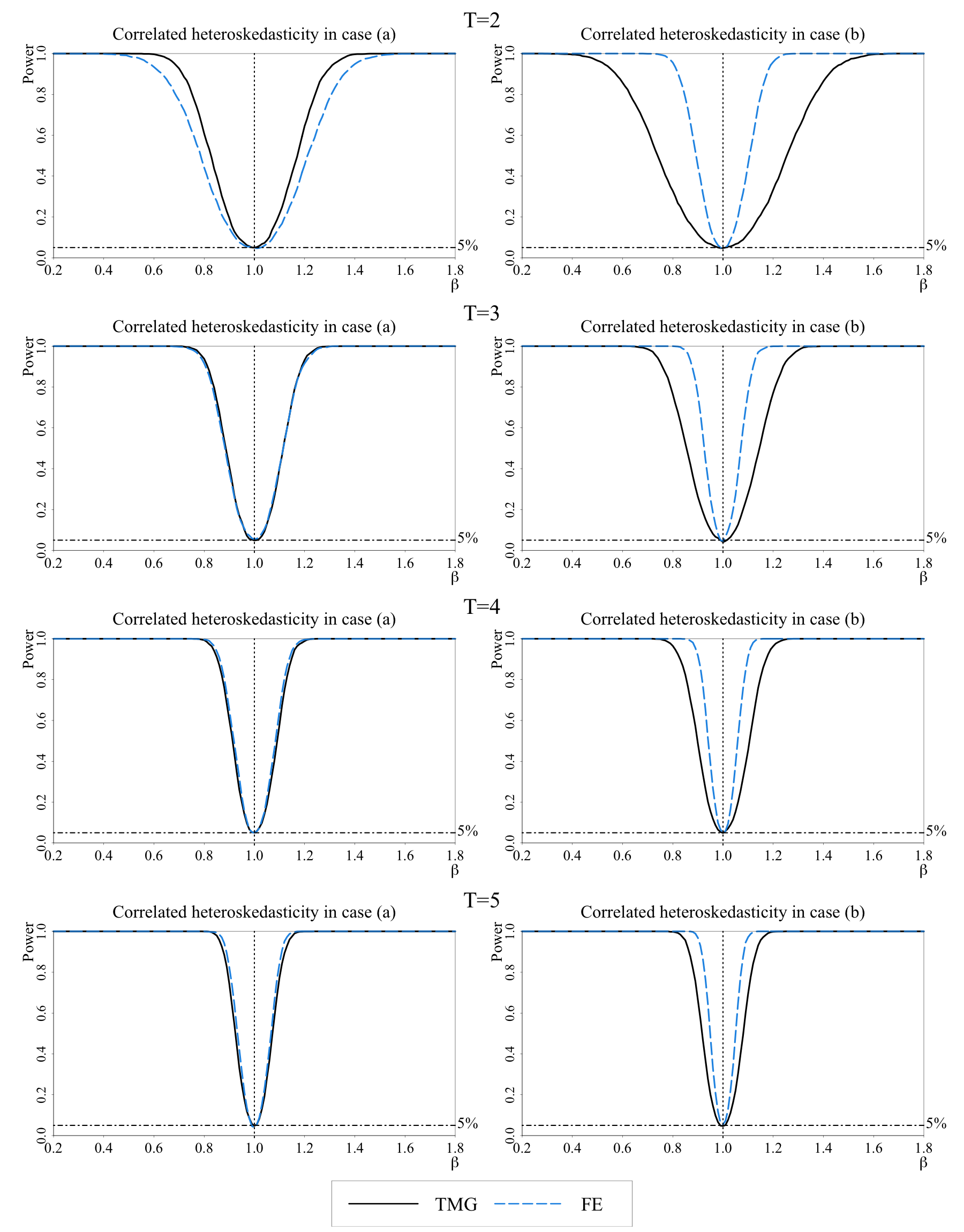
Figure S.1: Empirical power functions for FE and TMG estimators of $\beta_{0}$ $(E(\beta_{i})=\beta_{0}=1)$ in panel data models without time effects and with uncorrelated heterogeneity, $\rho_{\beta}=0$, and correlated heteroskedasticity (cases (a) and (b))

Notes: For details of the DGP for the left and right panels, see footnote (i) to Table S.3. For the FE estimator, see footnote (ii) to Table S.3. For the TMG estimator, see footnotes (ii) and (iii) to Table S.3.

Table S.4: Bias, RMSE and size of FE, MG and TMG estimators of $\beta_{0}$ $(E(\beta_{i})=\beta_{0}=1)$ in panel data models without time effects and with different degrees of correlated heterogeneity, $\rho_{\beta}$, and overall fit, $PR^{2}$

	(2) Medium correlated heterogeneity $\rho_{\beta}=0.25$ with $PR^{2}=0.2$														(4) Large correlated heterogeneity $\rho_{\beta}=0.5$ with $PR^{2}=0.4$
	$\hat{\pi}$ $(\times 100)$		Bias				RMSE				Size $(\times 100)$				$\hat{\pi}$ $(\times 100)$		Bias				RMSE				Size $(\times 100)$
$T$	TMG		FE	MG	TMG		FE	MG	TMG		FE	MG	TMG		TMG		FE	MG	TMG		FE	MG	TMG		FE	MG	TMG
	$n=1,000$
2	31.2		0.220	-7.516	0.023		0.28	362.16	0.34		26.2	2.1	4.5		31.2		0.445	-4.724	0.049		0.47	227.71	0.22		94.1	2.1	5.4
3	16.5		0.161	-0.011	0.010		0.20	0.58	0.20		26.8	4.0	4.8		16.5		0.322	-0.007	0.023		0.33	0.37	0.13		96.8	4.0	5.6
4	10.4		0.132	-0.001	0.006		0.16	0.21	0.15		29.4	5.2	5.2		10.4		0.266	0.000	0.014		0.28	0.13	0.09		96.7	5.1	5.4
5	7.1		0.114	0.000	0.005		0.14	0.14	0.12		28.8	4.2	3.9		7.1		0.230	0.000	0.009		0.24	0.09	0.07		96.9	4.0	4.3
6	5.2		0.106	0.000	0.004		0.13	0.11	0.10		30.4	4.6	4.9		5.2		0.210	0.000	0.007		0.22	0.07	0.06		96.7	4.9	5.1
8	3.2		0.091	0.000	0.002		0.11	0.08	0.08		29.8	4.5	4.6		3.2		0.179	0.000	0.004		0.19	0.05	0.05		96.6	4.8	4.2
	$n=2,000$
2	28.5		0.220	-2.449	0.021		0.25	153.07	0.26		42.2	2.0	5.4		28.5		0.446	-1.546	0.044		0.46	96.55	0.17		99.8	2.0	5.7
3	14.1		0.162	0.007	0.008		0.18	0.45	0.16		47.3	4.3	5.5		14.1		0.323	0.005	0.020		0.33	0.28	0.10		100.0	4.4	5.9
4	8.4		0.133	-0.003	0.002		0.15	0.15	0.11		50.6	4.5	4.5		8.4		0.265	-0.002	0.009		0.27	0.10	0.07		99.9	4.4	4.9
5	5.6		0.117	-0.004	0.003		0.13	0.11	0.09		51.0	5.1	5.2		5.6		0.233	-0.003	0.007		0.24	0.07	0.06		99.9	5.4	5.0
6	4.0		0.104	-0.001	0.002		0.12	0.08	0.07		50.3	4.0	4.2		4.0		0.208	0.000	0.005		0.21	0.05	0.05		100.0	4.1	4.0
8	2.4		0.089	0.000	0.001		0.10	0.06	0.06		50.9	5.0	4.6		2.4		0.178	0.000	0.003		0.18	0.04	0.04		100.0	4.8	4.2
	$n=5,000$
2	24.7		0.227	-4.227	0.019		0.24	419.33	0.18		81.6	1.8	4.2		24.7		0.451	-2.757	0.037		0.45	274.79	0.12		100.0	1.8	5.6
3	10.8		0.162	-0.006	0.008		0.17	0.29	0.10		84.7	4.7	5.0		10.8		0.323	-0.004	0.016		0.33	0.18	0.07		100.0	4.7	6.0
4	5.8		0.133	0.000	0.004		0.14	0.10	0.08		86.9	5.0	5.6		5.8		0.265	0.000	0.008		0.27	0.06	0.05		100.0	5.1	6.0
5	3.5		0.115	-0.001	0.002		0.12	0.07	0.06		85.9	4.4	4.2		3.5		0.231	-0.001	0.004		0.23	0.04	0.04		100.0	4.3	4.4
6	2.3		0.103	0.000	0.002		0.11	0.06	0.05		86.4	5.3	5.5		2.3		0.207	0.000	0.003		0.21	0.04	0.03		100.0	5.3	5.9
8	1.2		0.089	0.000	0.000		0.09	0.04	0.04		87.4	5.0	4.9		1.2		0.177	0.000	0.001		0.18	0.03	0.03		100.0	4.7	4.7
	$n=10,000$
2	22.1		0.224	-1.595	0.012		0.23	179.03	0.14		97.9	2.2	4.8		22.1		0.450	-0.990	0.030		0.45	113.06	0.09		100.0	2.2	6.9
3	8.8		0.160	0.004	0.006		0.16	0.20	0.07		98.4	4.3	5.2		8.8		0.321	0.003	0.013		0.32	0.13	0.05		100.0	4.3	6.1
4	4.4		0.132	0.000	0.004		0.14	0.07	0.05		99.1	4.7	4.7		4.4		0.265	0.000	0.007		0.27	0.04	0.03		100.0	4.9	4.9
5	2.5		0.115	-0.001	0.001		0.12	0.05	0.04		99.2	4.3	4.6		2.5		0.231	0.000	0.003		0.23	0.03	0.03		100.0	4.6	4.7
6	1.6		0.104	0.000	0.001		0.11	0.04	0.04		99.4	4.1	4.0		1.6		0.208	0.000	0.002		0.21	0.02	0.02		100.0	4.2	3.9
8	0.8		0.089	0.000	0.001		0.09	0.03	0.03		99.2	4.9	4.9		0.8		0.177	0.000	0.001		0.18	0.02	0.02		100.0	5.0	5.1

Notes: The data generating process is given by $y_{it}=\alpha_{i}+\beta_{i}x_{it}+\sigma_{it}e_{it}$ with random heteroskedasticity, different degrees of correlated heterogeneity, $\rho_{\beta}$ (defined by (8.6) in the main paper), and levels of overall fit, $PR^{2}$ (defined by (S.3.3)). The errors processes for $y_{it}$ and $x_{it}$ equations are chi-squared and Gaussian, respectively, and $x_{it}$ are generated as heterogeneous AR(1) processes. For further details see Section 8.1.3 in the main paper and Section S.3. For FE and MG estimators, see footnote (ii) to Table S.3. For the TMG estimator, see footnotes (ii) and (iii) to Table S.3. $\hat{\pi}$ is the simulated fraction of individual estimates being trimmed, defined by (4.7) in the main paper.

S.4.2 Comparison of TMG and GP estimators for different exponents, $\alpha$ and $\alpha_{GP},$ used in the threshold values

Table S.5 compares small sample properties of TMG and GP estimators of $\beta_{0}$ for different choices of $\alpha$ and $\alpha_{GP}$ used for their computations, respectively. The results are for the baseline model with correlated heterogeneity, but without time effects, for ultra short values of $T=2,3$, and $n=1,000$, $2,000$, $5,000$ and $10,000$. The empirical power functions for TMG and GP estimators are shown in Figures S.4 and S.5. The figures suggest that both estimators benefit from setting $\alpha$ and $2\alpha_{GP}$ close to $1/3$ value obtained from our theoretical derivations. The TMG estimator is less sensitive to the choice of $\alpha$ as compared to the $GP$ estimator to $\alpha_{GP}$. For further discussions see Section 8.2.4 of the main paper.

Table S.5: Bias, RMSE and size of TMG and GP estimators of $\beta_{0}$ $(E(\beta_{i})=\beta_{0}=1)$ for different values of the parameters, $\alpha$ and $\alpha_{GP}$, in the baseline model without time effects and with correlated heterogeneity, $\rho_{\beta}=0.5$

		$T=2$					$T=3$
		$\hat{\pi}$			Size		$\hat{\pi}$			Size
Estimator	$\alpha$/$\alpha_{GP}$	$(\times 100)$	Bias	RMSE	$(\times 100)$		$(\times 100)$	Bias	RMSE	$(\times 100)$
		$n=1,000$
TMG	1/3	31.2	0.048	0.35	4.9		16.5	0.023	0.20	5.2
TMG	0.35	29.6	0.045	0.36	4.6		15.0	0.020	0.21	5.0
TMG	1/2	18.1	0.017	0.47	5.7		6.0	0.004	0.25	4.7
GP	0.35/2	12.6	0.017	0.51	5.5		15.0	0.045	0.20	5.9
GP	1/4	7.5	0.001	0.64	5.4		6.0	0.014	0.23	5.6
GP	1/3	4.2	-0.029	0.83	4.5		1.4	0.011	0.31	4.5
		$n=2,000$
TMG	1/3	28.5	0.044	0.27	5.3		14.1	0.018	0.16	5.4
TMG	0.35	26.8	0.041	0.28	5.3		12.7	0.016	0.16	5.3
TMG	1/2	15.6	0.028	0.37	5.1		4.5	0.004	0.20	5.0
GP	0.35/2	11.2	0.023	0.38	4.9		12.7	0.035	0.16	6.1
GP	1/4	6.4	0.035	0.50	4.7		4.5	0.009	0.18	5.0
GP	1/3	3.4	0.031	0.70	5.8		0.9	-0.001	0.23	5.0
		$n=5,000$
TMG	1/3	24.7	0.037	0.18	4.7		10.8	0.016	0.11	5.3
TMG	0.35	23.1	0.034	0.19	4.4		9.5	0.014	0.11	5.1
TMG	1/2	12.4	0.016	0.26	4.6		2.9	0.002	0.14	5.2
GP	0.35/2	9.6	0.018	0.26	4.6		9.5	0.029	0.10	5.1
GP	1/4	5.1	0.012	0.36	4.7		2.9	0.008	0.13	4.7
GP	1/3	2.5	0.009	0.52	5.2		0.5	0.002	0.16	3.9
		$n=10,000$
TMG	1/3	22.1	0.029	0.14	5.6		8.8	0.013	0.08	5.3
TMG	0.35	20.6	0.025	0.15	5.3		7.7	0.011	0.08	4.9
TMG	1/2	10.5	0.009	0.21	4.7		2.1	0.002	0.10	4.8
GP	0.35/2	8.5	0.012	0.20	6.0		7.7	0.022	0.08	5.8
GP	1/4	4.3	-0.002	0.28	5.1		2.1	0.005	0.09	4.8
GP	1/3	2.0	0.002	0.41	4.3		0.3	0.001	0.12	5.2

Notes: (i) The GP estimator is given by (3.1) in the main paper. For $T=2$, GP compare $d_{i}^{1/2}$ with the bandwidth $h_{n}=C_{GP}n^{-\alpha_{GP}}$. $\alpha_{GP}$ is set to 1/3. $C_{GP}=\frac{1}{2}\min\left(\hat{\sigma}_{D},\hat{r}_{D}/1.34\right)$, where $\hat{\sigma}_{D}$ and $\hat{r}_{D}$ are the respective sample standard deviation and interquartile range of $\mathop{\mathrm{d}et}(\boldsymbol{W}_{i})$. For $T=3$, we continue using the bandwidth $h_{n}$ with $C_{GP}=(\bar{d}_{n})^{1/2}$. See Section 8.2.2 in the main paper for details. (ii) For details of the baseline model, see footnote (i) to Table 1 in the main paper. For the TMG estimator and its threshold, see footnotes (ii) and (iii) to Table S.3. $\hat{\pi}$ is the simulated fraction of individual estimates being trimmed, defined by (4.7) in the main paper.

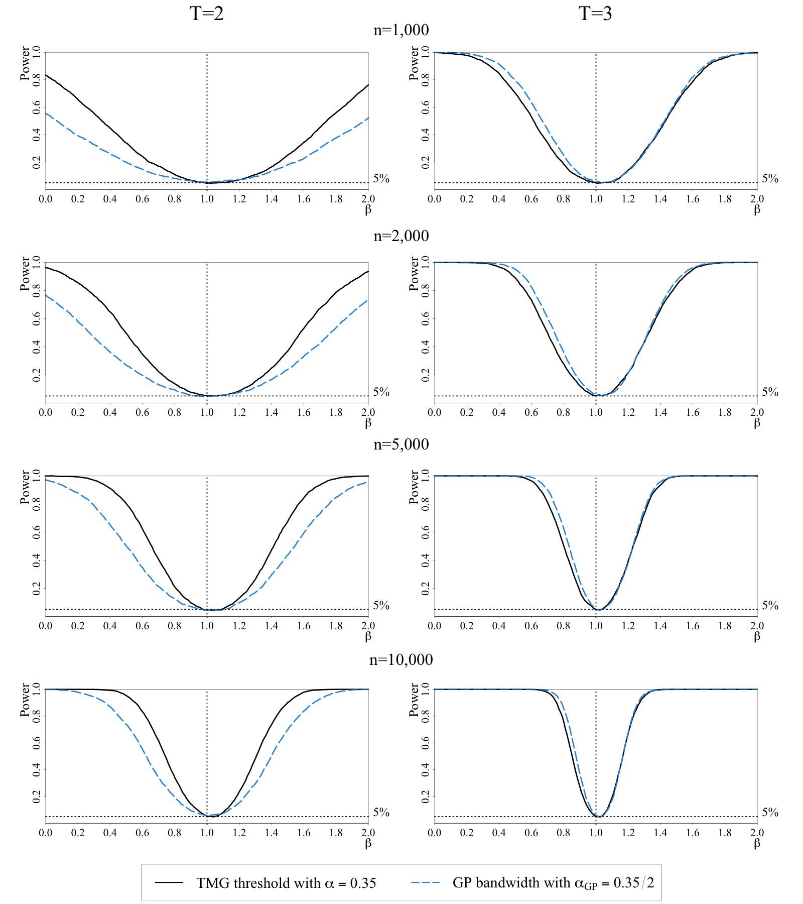
Figure S.2: Empirical power functions for TMG and GP estimator of $\beta_{0}$ $(E(\beta_{i})=\beta_{0}=1)$ for parameters $\alpha=0.35$ and $\alpha_{GP}=0.35/2$ in the baseline model without time effects and with correlated heterogeneity, $\rho_{\beta}=0.5$

Notes: For details of the baseline model without time effects, see footnote (i) to Table 1 in the main paper. See also footnotes (ii) and (iii) to Table S.3 and footnote (i) to Table S.5.

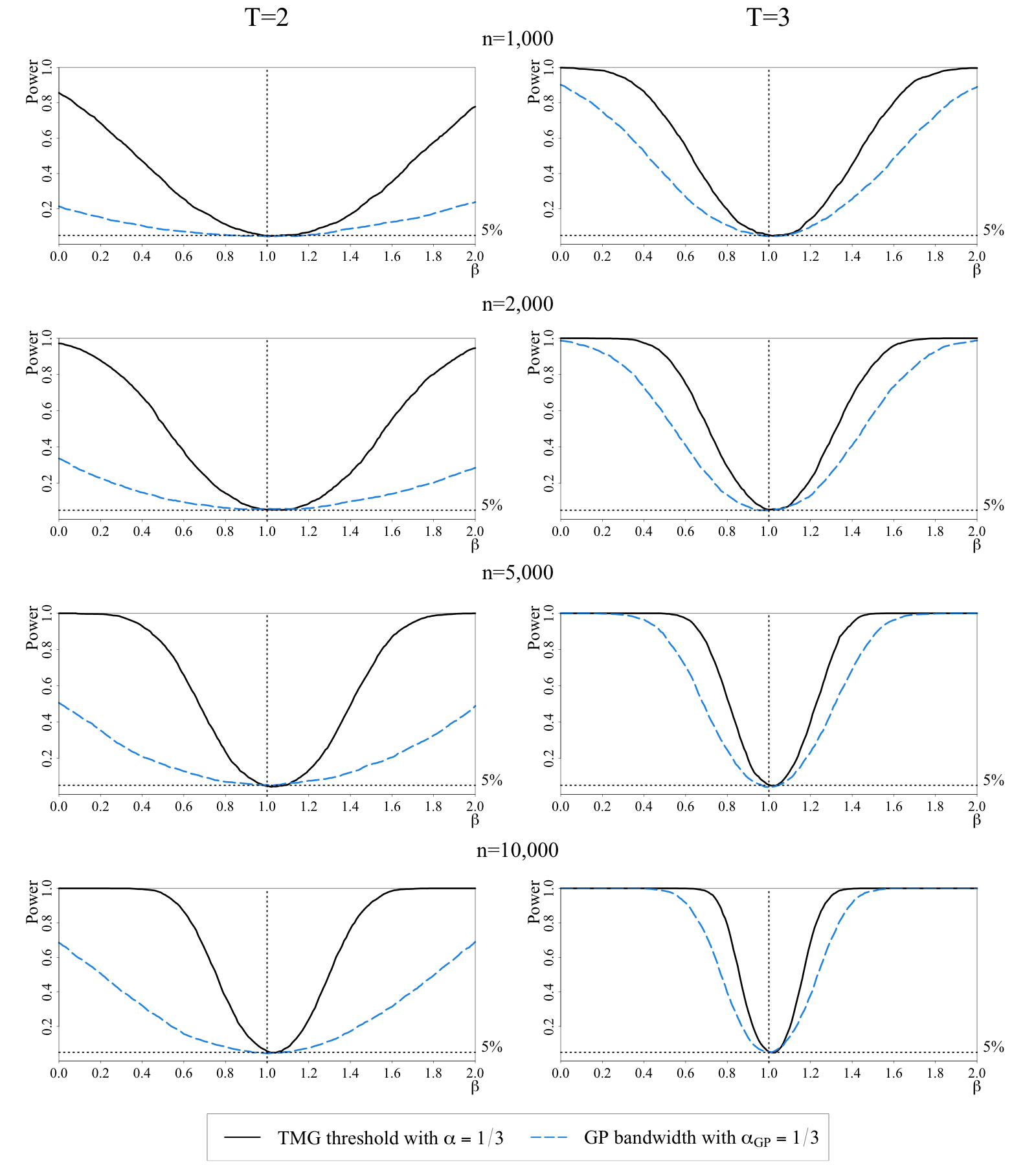
Figure S.3: Empirical power functions for TMG and GP estimator of $\beta_{0}$ $(E(\beta_{i})=\beta_{0}=1)$ for parameters $\alpha=1/3$ and $\alpha_{GP}=1/3$ in the baseline model without time effects and with correlated heterogeneity, $\rho_{\beta}=0.5$

Notes: For details of the baseline model without time effects, see footnote (i) to Table 1 in the main paper. See also footnotes (ii) and (iii) to Table S.3 and footnote (i) to Table S.5.

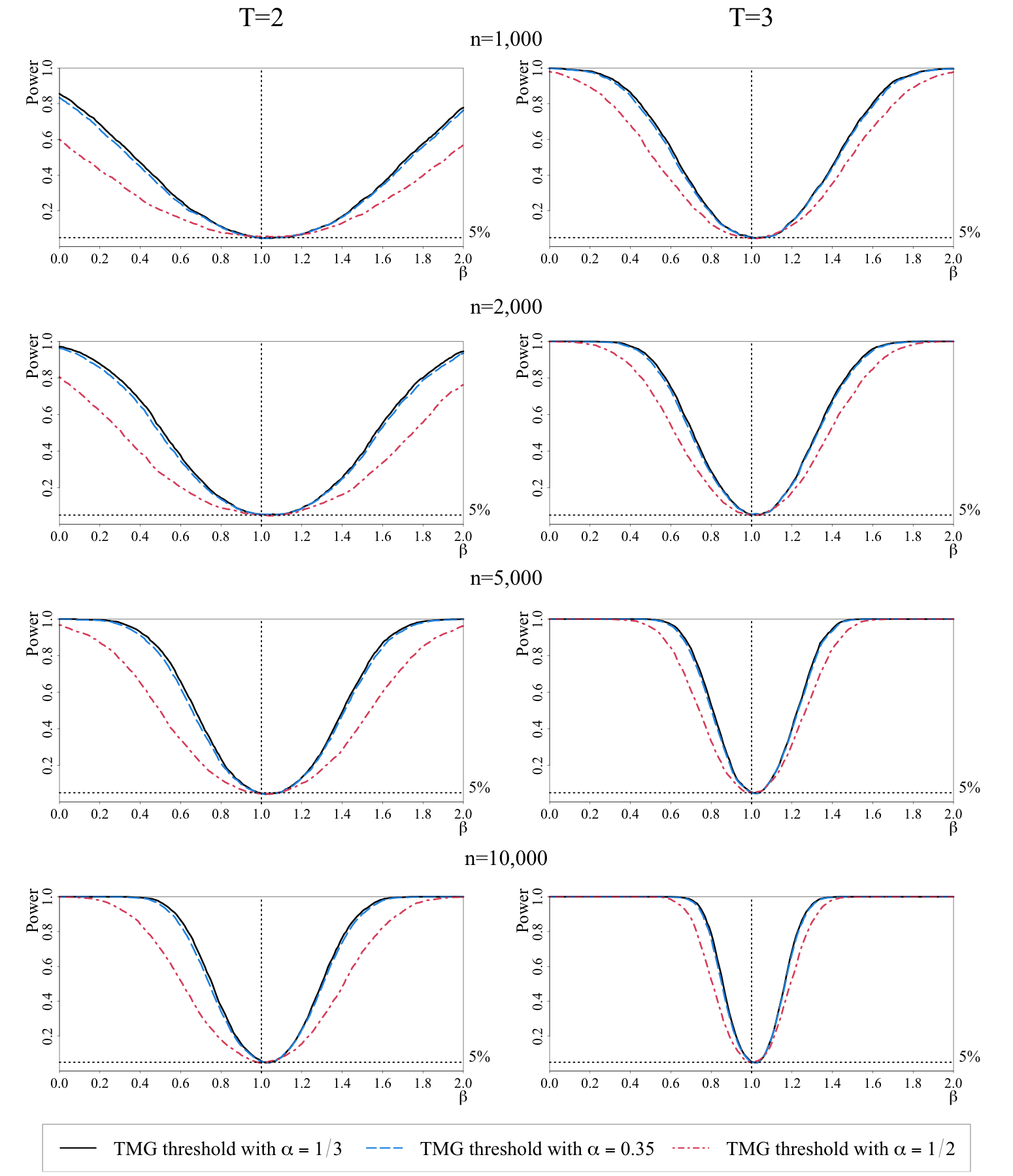
Figure S.4: Empirical power functions for the TMG estimator of $\beta_{0}$ $(E(\beta_{i})=\beta_{0}=1)$ for different values of the threshold parameter, $\alpha\in\{1/3,0.35,1/2\}$, in the baseline model without time effects and with correlated heterogeneity, $\rho_{\beta}=0.5$

Notes: For details of the baseline model without time effects, see footnote (i) to Table 1 in the main paper. See also footnotes (ii) and (iii) to Table S.3.

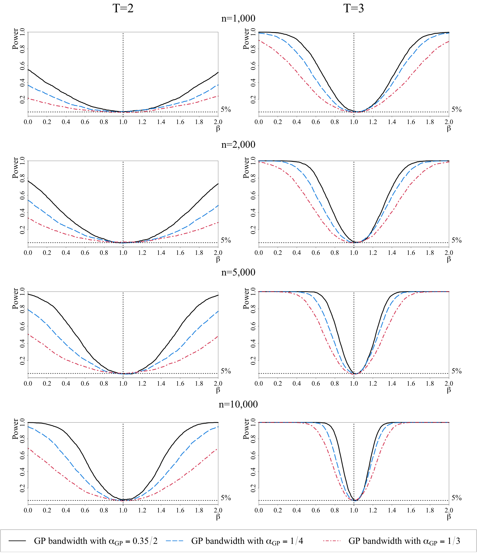
Figure S.5: Empirical power functions for the GP estimator of $\beta_{0}$ $(E(\beta_{i})=\beta_{0}=1)$ for different values of the bandwidth parameter, $\alpha_{GP}\in\{0.35/2,1/4,1/3\}$ in the baseline model without time effects and with correlated heterogeneity, $\rho_{\beta}=0.5$

Notes: For details of the baseline model without time effects, see footnote (i) to Table 1 in the main paper. See also footnote (i) to Table S.5.

S.4.3 Comparison of TMG and GP estimators with correlated heteroskedasticity

Table S.6 provides additional MC results on small sample properties of TMG and GP estimators of $\beta_{0}$ in panel data models with correlated heterogeneity, $\rho_{\beta}=0.5$, as well as correlated error heteroskedasticity which are generated as case (a) $\sigma_{it}^{2}=\lambda_{i}^{2}$, and case (b) $\sigma_{it}^{2}=e_{x,it}^{2}$, for all $i$ and $t$. These results are to be compared to the ones in Table 2 in Section 8.2.2 of the main paper which are for random heteroskedasticity. The TMG estimator continues to perform better than the GP estimator when $T=2$ or $3$, and allowing for correlated heteroskedasticity does not alter this conclusion.

Table S.6: Bias, RMSE and size of TMG and GP estimators of $\beta_{0}$ $(E(\beta_{i})=\beta_{0}=1)$ in panel data models without time effects and with correlated heterogeneity, $\rho_{\beta}=0.5$, and correlated heteroskedasticity (cases (a) and (b))

		$T=2$					$T=3$
		$\hat{\pi}$			Size		$\hat{\pi}$			Size
Estimator		$(\times 100)$	Bias	RMSE	$(\times 100)$		$(\times 100)$	Bias	RMSE	$(\times 100)$
Case (a): $\sigma_{it}^{2}=\lambda_{i}^{2}$
	$n=1,000$
TMG		31.2	0.049	0.25	5.4		16.5	0.023	0.16	4.9
GP		4.2	-0.012	0.53	4.7		2.0	0.000	0.22	4.3
	$n=2,000$
TMG		28.5	0.044	0.19	5.6		14.1	0.018	0.13	5.7
GP		3.4	0.022	0.46	6.0		1.3	0.004	0.18	5.2
	$n=5,000$
TMG		24.7	0.036	0.13	4.5		10.8	0.016	0.09	5.5
GP		2.5	0.000	0.33	5.4		0.7	0.000	0.13	5.4
	$n=10,000$
TMG		22.1	0.031	0.10	6.3		8.8	0.014	0.06	5.1
GP		2.0	0.004	0.25	4.3		0.5	0.000	0.09	4.9
Case (b): $\sigma_{it}^{2}=e_{x,it}^{2}$
	$n=1,000$
TMG		31.2	0.050	0.37	5.5		16.5	0.024	0.21	5.1
GP		4.2	-0.018	0.85	5.1		2.0	-0.003	0.28	4.6
	$n=2,000$
TMG		28.5	0.043	0.28	5.7		14.1	0.020	0.16	5.1
GP		3.4	0.038	0.72	5.4		1.3	0.003	0.22	4.7
	$n=5,000$
TMG		24.7	0.033	0.19	4.8		10.8	0.014	0.11	5.3
GP		2.5	-0.007	0.53	5.9		0.7	-0.002	0.15	4.3
	$n=10,000$
TMG		22.1	0.032	0.14	5.7		8.8	0.013	0.08	5.5
GP		2.0	0.006	0.41	5.3		0.5	-0.001	0.11	4.5

Notes: (i) The data generating process is given by $y_{it}=\alpha_{i}+\beta_{i}x_{it}+\sigma_{it}e_{it}$, where $\sigma_{it}^{2}$ are generated as case (a): $\sigma_{it}^{2}=\lambda_{i}^{2}$, and case (b): $\sigma_{it}^{2}=e_{x,it}^{2}$, for all $i$ and $t$. The errors processes for $y_{it}$ and $x_{it}$ equations are chi-squared and Gaussian, respectively. $x_{it}$ are generated as heterogeneous AR(1) processes. $\rho_{\beta}$ is defined by (8.6) in the main paper. For further details see Section 8.1.3 in the main paper and Section S.3. (ii) For the TMG estimator, see footnotes (ii) and (iii) to Table S.3. For the GP estimator, see footnote (i) to Table S.5. $\hat{\pi}$ is the simulated fraction of individual estimates being trimmed, given by (4.7) in the main paper.

Appendix S.5 The effects of increasing $PR^{2}$ on the small sample properties of TMG, TMG-TE and TMG-C, GP and SU estimators

Table S.7 provides summary MC results with the higher level of fit, $PR^{2}=0.4$, for $T=2$ and $3$ and $n=1,000$, $2,000$, $5,000$, $10,000$. These results are comparable with the ones reported in Table 2 for the baseline model where $PR^{2}=0.2$. Table S.8 gives the same results for $\beta_{0}$ but under DGPs with time effects, and Table S.9 provides the results for the time effect $\phi_{1}$ when $T=2,$ and the time effects, $\phi_{1}$ and $\phi_{2}$, when $T=3$.

Table S.10 reports bias, RMSE and size for the TMG and GP estimators for models with and without time effects, and for different $x_{it}$ processes, for $T=2$ and $n=1,000$, $2,000$, $5,000$, $10,000$.

Table S.7: Bias, RMSE and size of TMG, GP and SU estimators of $\beta_{0}$ $(E(\beta_{i})=\beta_{0}=1)$ in panel data models without time effects and with correlated heterogeneity, $\rho_{\beta}=0.5$, and the level of overall fit, $PR^{2}=0.4$

		$T=2$					$T=3$
		$\hat{\pi}$			Size		$\hat{\pi}$			Size
Estimator		$(\times 100)$	Bias	RMSE	$(\times 100)$		$(\times 100)$	Bias	RMSE	$(\times 100)$
	$n=1,000$
TMG		31.2	0.049	0.22	5.4		16.5	0.023	0.13	5.6
GP		4.2	-0.014	0.51	4.6		2.0	0.001	0.17	4.7
SU		4.2	-0.028	0.99	4.9		…	…	…	…
	$n=2,000$
TMG		28.5	0.044	0.17	5.7		14.1	0.020	0.10	5.9
GP		3.4	0.022	0.43	5.8		1.3	0.004	0.13	4.7
SU		3.4	0.005	0.85	5.5		…	…	…	…
	$n=5,000$
TMG		24.7	0.037	0.12	5.6		10.8	0.016	0.07	6.0
GP		2.5	0.007	0.32	5.3		0.7	0.000	0.09	5.1
SU		2.5	0.002	0.62	4.9		…	…	…	…
	$n=10,000$
TMG		22.1	0.030	0.09	6.9		8.8	0.013	0.05	6.1
GP		2.0	0.003	0.25	4.4		0.5	0.000	0.07	4.9
SU		2.0	0.004	0.50	5.1		…	…	…	…

Notes: (i) The data generating process is given by $y_{it}=\alpha_{i}+\beta_{i}x_{it}+\sigma_{it}e_{it}$ with random heteroskedasticity, $\rho_{\beta}$ is defined by (8.6) in the main paper, and $PR^{2}$ is defined by (S.3.3). The errors processes for $y_{it}$ and $x_{it}$ equations are chi-squared and Gaussian, respectively, and $x_{it}$ are generated as heterogeneous AR(1) processes. For further details see Section 8.1.3 in the main paper and Section S.3. (ii) For the TMG estimator, see footnotes (ii) and (iii) to Table S.3. For the GP estimator, see footnote (i) to Table S.5. The SU estimator is proposed by Sasaki and Ura (2021), with the same threshold as the GP estimator. $\hat{\pi}$ is the simulated fraction of individual estimates being trimmed, defined by (4.7) in the main paper. The estimation algorithm for the SU estimator is not available for $T=3$, denoted by “…”.

Table S.8: Bias, RMSE and size of TMG-TE, TMG-C, GP and SU estimators of $\beta_{0}$ $(E(\beta_{i})=\beta_{0}=1)$ in panel data models with time effects, correlated heterogeneity, $\rho_{\beta}=0.5$, and the level of overall fit, $PR^{2}=0.4$

		$T=2$					$T=3$
		$\hat{\pi}$			Size		$\hat{\pi}$			Size
Estimator		$(\times 100)$	Bias	RMSE	$(\times 100)$		$(\times 100)$	Bias	RMSE	$(\times 100)$
	$n=1,000$
TMG-TE		31.2	0.049	0.22	5.5		16.5	0.023	0.13	5.6
TMG-C		…	…	…	…		16.5	0.023	0.13	5.5
GP		4.2	-0.018	0.52	4.0		2.0	0.001	0.17	4.6
SU		4.2	-0.032	1.02	5.4		…	…	…	…
	$n=2,000$
TMG-TE		28.5	0.044	0.17	5.6		14.1	0.020	0.10	5.7
TMG-C		…	…	…	…		14.1	0.020	0.10	5.7
GP		3.4	0.022	0.44	5.2		1.3	0.004	0.13	4.7
SU		3.4	0.007	0.86	5.8		…	…	…	…
	$n=5,000$
TMG-TE		24.7	0.037	0.12	5.6		10.8	0.016	0.07	6.0
TMG-C		…	…	…	…		10.8	0.016	0.07	6.0
GP		2.5	0.007	0.32	5.0		0.7	0.000	0.09	5.1
SU		2.5	0.004	0.63	4.7		…	…	…	…
	$n=10,000$
TMG-TE		22.1	0.030	0.09	6.9		8.8	0.013	0.05	6.1
TMG-C		…	…	…	…		8.8	0.013	0.05	6.1
GP		2.0	0.003	0.25	4.3		0.5	0.000	0.07	4.9
SU		2.0	0.007	0.50	5.4		…	…	…	…

Notes: (i) The data generating process is given by $y_{it}=\alpha_{i}+\beta_{i}x_{it}+\sigma_{it}e_{it}$ with random heteroskedasticity, $\rho_{\beta}$ is defined by (8.6) in the main paper, and $PR^{2}$ is defined by (S.3.3). Time effects are set as $\phi_{t}=t$ for $t=1,2,...,T-1$, and $\phi_{T}=-T(T-1)/2$. The errors processes for $y_{it}$ and $x_{it}$ equations are chi-squared and Gaussian, respectively, and $x_{it}$ are generated as heterogeneous AR(1) processes. For further details see Section 8.1.3 in the main paper and Section S.3. (ii) The TMG-TE estimators of $\boldsymbol{\theta}_{0}$ and $\boldsymbol{\phi}$ are given by (6.9) and (6.11) in the main paper, respectively, and their asymptotic variances are given by (A.3.4) and (A.3.7), respectively. The TMG-C estimators of $\boldsymbol{\theta}_{0}$ and $\boldsymbol{\phi}$ are given by (6.20) and (6.17) in the main paper, respectively, and their asymptotic variances are given by (6.21) and (6.19) in the main paper, respectively. For the trimming threshold, see footnote (iii) to Table S.3. (iii) GP and SU estimators are proposed by Graham and Powell (2012) and Sasaki and Ura (2021). For their trimming threshold, see footnote (i) to Table S.5. $\hat{\pi}$ is the simulated fraction of individual estimates being trimmed, defined by (4.7) in the main paper. “…” denotes the estimation algorithms are not available or not applicable.

Table S.9: Bias, RMSE and size of TMG-TE and GP estimators of the time effects, $\phi_{1}$ and $\phi_{2}$, in panel data model with correlated heterogeneity, $\rho_{\beta}=0.5$, and the overall fit, $PR^{2}=0.4$

				$n=1,000$				$n=5,000$
		Estimator		Bias	RMSE	Size $(\times 100)$		Bias	RMSE	Size $(\times 100)$
					$T=2$				$T=2$
$\phi_{1}=1$		TMG-TE		0.002	0.06	6.1		-0.001	0.02	4.7
		GP		0.001	0.33	7.1		-0.005	0.21	6.9
					$T=3$				$T=3$
$\phi_{1}=1$		TMG-TE		0.165	0.00	6.5		0.108	0.00	2.9
		GP		0.020	0.00	9.1		0.007	0.00	4.1
$\phi_{2}=2$		TMG-TE		0.165	0.00	6.5		0.108	0.00	2.9
		GP		0.020	-0.01	8.1		0.007	0.00	3.7

Notes: See the notes to Table S.8.

Table S.10: Bias, RMSE and size of TMG, GP and TMG-TE estimators of $\beta_{0}$ $(E(\beta_{i})=\beta_{0}=1)$ under different model specifications with correlated heterogeneity, $\rho_{\beta}=0.5$, and the level of overall fit, $PR^{2}=0.2$, for $T=2$

		$n=1,000$					$n=2,000$					$n=5,000$					$n=10,000$
		$\hat{\pi}$			Size		$\hat{\pi}$			Size		$\hat{\pi}$			Size		$\hat{\pi}$			Size
Estimator		$(\times 100)$	Bias	RMSE	$(\times 100)$		$(\times 100)$	Bias	RMSE	$(\times 100)$		$(\times 100)$	Bias	RMSE	$(\times 100)$		$(\times 100)$	Bias	RMSE	$(\times 100)$
I. Without time effects in $y_{it}$
(a) Gaussian errors in $y_{it}$
TMG		27.3	0.051	0.263	5.3		24.5	0.057	0.200	5.7		21.1	0.039	0.139	6.2		18.9	0.034	0.108	7.3
GP		4.0	0.015	0.558	4.6		3.2	0.024	0.448	4.2		2.4	0.001	0.343	5.6		1.9	0.002	0.274	5.6
(b) Chi-squared errors in $y_{it}$
TMG		27.3	0.051	0.260	5.8		24.5	0.049	0.199	5.1		21.1	0.039	0.138	5.8		18.9	0.033	0.105	6.2
GP		4.0	0.008	0.569	4.9		3.2	0.012	0.451	4.8		2.4	0.003	0.338	4.7		1.9	-0.003	0.267	4.7
(c) Heterogeneous AR(1) $x_{it}$ processes
TMG		31.2	0.048	0.353	4.9		28.5	0.044	0.272	5.3		24.7	0.037	0.184	4.7		22.1	0.029	0.143	5.6
GP		4.2	-0.029	0.830	4.5		3.4	0.031	0.701	5.8		2.5	0.009	0.523	5.2		2.0	0.002	0.408	4.3
(d) Heterogeneous AR(1) $x_{it}$ processes with interactive effects
TMG		29.9	0.037	0.413	5.4		26.9	0.028	0.309	4.7		23.4	0.025	0.213	5.1		20.8	0.019	0.162	5.7
GP		4.2	-0.017	0.938	4.9		3.3	0.002	0.765	4.8		2.5	0.017	0.584	5.4		1.9	-0.010	0.459	4.8
II. With time effects in $y_{it}$
(a) Chi-squared errors in $y_{it}$
TMG-TE		27.3	0.055	0.256	4.9		24.5	0.060	0.209	7.1		21.2	0.038	0.141	6.8		18.9	0.038	0.109	7.2
GP		4.1	-0.005	0.588	4.8		3.2	0.026	0.456	4.2		2.4	-0.001	0.356	5.4		1.9	0.009	0.271	5.4
(b) Heterogeneous AR(1) $x_{it}$ processes
TMG-TE		31.2	0.048	0.353	5.0		28.5	0.044	0.272	5.6		24.7	0.037	0.184	4.7		22.1	0.028	0.143	5.7
GP		4.2	-0.034	0.844	3.9		3.4	0.032	0.712	5.2		2.5	0.008	0.527	5.0		2.0	0.003	0.410	4.4
(c) Heterogeneous AR(1) $x_{it}$ processes with interactive effects
TMG-TE		29.9	0.037	0.433	5.2		26.9	0.029	0.319	4.2		23.4	0.026	0.220	4.9		20.8	0.020	0.167	5.5
GP		4.2	-0.017	0.968	4.4		3.3	-0.004	0.791	4.4		2.5	0.014	0.592	4.7		1.9	-0.008	0.470	4.7

Notes: (i) The data generating process is given by $y_{it}=\alpha_{i}+\phi_{t}+\beta_{i}x_{it}+\sigma_{it}e_{it}$ with random heteroskedasticity. Time effects are set as $\phi_{t}=t$ for $t=1,2,...,T-1$, and $\phi_{T}=-T(T-1)/2$. For further details see Section 8.1.3 in the main paper and Section S.3. (ii) For the TMG estimator, see footnote (ii) to Table S.3. For the GP estimator, see footnote (i) to Table S.5. For the TMG-TE estimator, see footnote (ii) to Table S.8. $\hat{\pi}$ is the simulated fraction of individual estimates being trimmed, defined by (4.7) in the main paper.

Appendix S.6 Monte Carlo evidence when the errors of $x_{it}$ are uniformly distributed

In this section, the DGP is generated using the baseline model without time effects, but with the errors in the $x_{it}$ equation drawn from a uniform distribution, as compared to the Gaussian errors used in the baseline model. Table S.11 compares small sample performance of the TMG estimator of $\beta_{0}$ using different $\alpha\in\{1/3,0.35,1/2\}$ for threshold values with correlated heterogeneity, $\rho_{\beta}=0.5$ for $T=2,3$, and $n=1,000$, $2,000$, $5,000$ and $10,000$. Table S.12 reports bias, RMSE and size of FE, MG and TMG estimators of $\beta_{0}$ for $T=2,3,4,5,6,8$, and $n=1,000$, $2,000$, $5,000$ and $10,000$.

The choice of the error distribution does not seem to be consequential.

Table S.11: Bias, RMSE and size of the TMG estimator of $\beta_{0}$ $(E(\beta_{i})=\beta_{0}=1)$ for different values of the threshold parameter, $\alpha$, in the baseline model without time effects and with correlated heterogeneity, $\rho_{\beta}=0.5$, using uniformly distributed errors in the $x_{it}$ equation

		$T=2$					$T=3$
		$\hat{\pi}$			Size		$\hat{\pi}$			Size
Estimator	$\alpha$	$(\times 100)$	Bias	RMSE	$(\times 100)$		$(\times 100)$	Bias	RMSE	$(\times 100)$
		$n=1,000$
TMG	1/3	27.0	0.051	0.33	5.0		12.6	0.027	0.20	5.2
TMG	0.35	25.5	0.048	0.34	5.0		11.3	0.025	0.20	5.3
TMG	0.50	15.2	0.025	0.43	4.4		4.0	0.012	0.23	4.9
		$n=2,000$
TMG	1/3	24.4	0.045	0.26	5.2		10.5	0.024	0.15	5.6
TMG	0.35	22.9	0.042	0.27	5.2		9.3	0.022	0.15	5.1
TMG	0.50	13.0	0.024	0.34	5.0		3.0	0.012	0.18	5.1
		$n=5,000$
TMG	1/3	20.9	0.041	0.18	6.0		7.7	0.015	0.10	5.0
TMG	0.35	19.5	0.038	0.19	5.9		6.7	0.013	0.10	5.3
TMG	0.50	10.3	0.020	0.25	5.0		1.9	0.006	0.12	4.9
		$n=10,000$
TMG	1/3	18.7	0.036	0.13	5.8		6.2	0.011	0.07	5.0
TMG	0.35	17.4	0.034	0.14	5.8		5.3	0.009	0.07	5.2
TMG	0.50	8.7	0.024	0.19	4.2		1.3	0.002	0.09	5.0

Notes: (i) The baseline model is generated as $y_{it}=\alpha_{i}+\beta_{i}x_{it}+u_{it}$, where the errors processes for $y_{it}$ and $x_{it}$ equations are chi-squared and uniformly distributed, respectively, $x_{it}$ are generated as heterogeneous AR(1) processes, and $\rho_{\beta}$ is defined by (8.6) in the main paper. For further details see Section 8.1.3 in the main paper and Section S.3. (ii) For the TMG estimator and its threshold, see footnotes (ii) and (iii) to Table S.3. $\hat{\pi}$ is the simulated fraction of individual estimates being trimmed, defined by (4.7) in the main paper.

Table S.12: Bias, RMSE and size of FE, MG and TMG estimators of $\beta_{0}$ $(E(\beta_{i})=\beta_{0}=1)$ in the baseline model without time effects, using uniformly distributed errors in the $x_{it}$ equation

	Uncorrelated heterogeneity: $\rho_{\beta}=0$														Correlated heterogeneity: $\rho_{\beta}=0.5$
	$\hat{\pi}$ $(\times 100)$		Bias				RMSE				Size $(\times 100)$				$\hat{\pi}$ $(\times 100)$		Bias				RMSE				Size $(\times 100)$
$T$	TMG		FE	MG	TMG		FE	MG	TMG		FE	MG	TMG		TMG		FE	MG	TMG		FE	MG	TMG		FE	MG	TMG
$n=1,000$
2	27.0		0.003	-4.499	0.001		0.17	188.74	0.31		5.5	2.0	4.8		27.0		0.367	-4.535	0.051		0.40	190.25	0.32		60.1	2.0	5.2
3	12.6		0.002	-0.015	0.005		0.11	0.61	0.19		4.7	4.3	5.3		12.6		0.243	-0.015	0.027		0.27	0.62	0.19		57.6	4.6	5.1
4	7.3		0.000	0.005	0.003		0.09	0.17	0.13		5.2	4.8	4.7		7.3		0.189	0.004	0.014		0.21	0.17	0.14		54.1	4.8	5.1
5	4.8		-0.003	0.000	-0.001		0.08	0.12	0.11		6.2	5.3	5.4		4.8		0.158	0.000	0.005		0.18	0.12	0.11		50.6	5.3	5.7
6	3.4		-0.001	-0.002	-0.001		0.07	0.10	0.09		4.3	5.5	5.2		3.4		0.142	-0.001	0.003		0.16	0.10	0.09		51.7	5.5	5.6
8	2.1		-0.002	-0.001	0.000		0.06	0.08	0.08		5.4	5.6	5.4		2.1		0.117	0.000	0.002		0.13	0.08	0.08		48.9	5.6	5.1
$n=2,000$
2	24.4		-0.003	1.103	0.002		0.12	69.57	0.24		4.9	2.0	5.0		24.4		0.361	1.112	0.045		0.38	70.12	0.25		84.0	2.0	5.2
3	10.5		0.000	0.003	0.006		0.08	0.45	0.14		5.6	5.1	5.1		10.5		0.240	0.003	0.024		0.25	0.46	0.14		81.9	5.1	5.6
4	5.7		0.000	0.003	0.002		0.06	0.13	0.10		4.2	4.8	4.7		5.7		0.188	0.003	0.010		0.20	0.13	0.10		81.3	4.6	4.6
5	3.6		-0.002	-0.006	-0.005		0.06	0.09	0.08		5.1	4.6	4.6		3.6		0.159	-0.006	0.000		0.17	0.09	0.08		77.8	4.4	4.6
6	2.6		-0.001	-0.002	-0.002		0.05	0.08	0.07		4.9	5.9	6.2		2.6		0.140	-0.002	0.001		0.15	0.08	0.07		78.1	5.9	6.0
8	1.5		0.000	-0.001	-0.001		0.04	0.06	0.06		4.7	5.1	5.1		1.5		0.118	-0.001	0.001		0.13	0.06	0.06		77.9	5.2	5.3
$n=5,000$
2	20.9		0.001	-0.277	0.004		0.07	171.87	0.17		4.5	2.2	5.1		20.9		0.365	-0.279	0.041		0.37	173.24	0.17		99.7	2.2	6.1
3	7.7		0.001	0.002	0.001		0.05	0.25	0.10		5.4	3.9	4.6		7.7		0.240	0.003	0.015		0.25	0.25	0.10		99.6	3.8	5.0
4	3.6		0.002	0.000	0.001		0.04	0.08	0.07		5.2	5.1	4.5		3.6		0.190	0.000	0.007		0.19	0.08	0.07		99.4	5.0	4.7
5	2.1		0.000	0.001	0.001		0.04	0.06	0.05		3.9	5.4	4.7		2.1		0.160	0.001	0.004		0.16	0.06	0.05		99.2	5.1	4.8
6	1.3		0.000	0.000	0.000		0.03	0.05	0.05		5.1	5.1	4.9		1.3		0.141	0.000	0.001		0.14	0.05	0.05		99.3	4.9	4.4
8	0.7		0.000	-0.001	-0.001		0.03	0.04	0.04		5.3	4.9	4.5		0.7		0.118	-0.001	0.000		0.12	0.04	0.04		98.9	5.0	4.6
$n=10,000$
2	18.7		0.000	5.925	0.003		0.06	223.71	0.12		5.8	2.5	4.8		18.7		0.366	5.972	0.036		0.37	225.49	0.13		100.0	2.5	5.9
3	6.2		0.000	-0.006	0.000		0.04	0.21	0.07		4.1	4.9	4.7		6.2		0.239	-0.006	0.011		0.24	0.21	0.07		100.0	4.8	5.0
4	2.6		0.000	0.002	0.000		0.03	0.06	0.05		5.4	5.6	5.6		2.6		0.189	0.002	0.004		0.19	0.06	0.05		100.0	5.2	5.6
5	1.4		0.000	0.001	0.001		0.03	0.04	0.04		4.2	4.9	5.6		1.4		0.160	0.001	0.003		0.16	0.04	0.04		100.0	5.3	5.2
6	0.8		0.000	0.000	0.000		0.02	0.03	0.03		5.0	5.0	5.2		0.8		0.142	0.000	0.001		0.14	0.03	0.03		100.0	5.0	5.3
8	0.4		0.000	0.001	0.001		0.02	0.03	0.03		4.9	4.4	4.6		0.4		0.119	0.001	0.001		0.12	0.03	0.03		100.0	4.3	4.3

Notes: (i) For details of the baseline model, see footnote (i) to Table S.11. (ii) For FE and MG estimators, see footnote (ii) to Table S.3. For the TMG estimator and its threshold, see footnotes (ii) and (iii) to Table S.3. $\hat{\pi}$ is the simulated fraction of individual estimates being trimmed, defined by (4.7) in the main paper.

Appendix S.7 Monte Carlo evidence of estimation with interactive effects in the regressor

To further examine the robustness of TMG-TE and TMG-C estimators to the choice of DGP, we generate the regressor, $x_{it}$, with interactive effects, namely

$$x_{it}=\alpha_{ix}(1-\rho_{ix})+\gamma_{ix}f_{t}+\rho_{ix}x_{i,t-1}+\left(1-\rho_{ix}^{2}\right)^{1/2}u_{x,it},$$

where $\gamma_{ix}\sim IIDU(0,2)$, $f_{t}=0.9f_{t-1}+(1-0.9^{2})^{1/2}v_{t},$ and $v_{t}\sim IIDN(0,1)$ for $t=-49,-48,...$, $-1,0,1,...,T$, with $f_{-50}=0$. We also calibrate $\kappa$ in the outcome equation given by (8.1) in the main paper, to achieve $PR^{2}=0.2$ by stochastic simulation (see Table S.2). The rest of the parameters are set as in the baseline model. See Section 8.1.3 in the main paper for details.

Tables S.13–S.14 summarize the results for TMG-TE, TMG-C, GP and SU estimators of $\beta_{0}$ and the time effect $\phi_{1}$ when $T=2,$ and the time effects $\phi_{1}$ and $\phi_{2}$ when $T=3$, for $T=2,3$ and $n=1,000$, $2,000$, $5,000$ and $10,000$.

The comparative performance of TMG-TE and GP estimators is unaffected by the addition of interactive effects to the $x_{it}$ process. The inclusion of interactive effects, by increasing the variance of $x_{it}$, results in improved estimates with a higher degree of precision, and a smaller number of estimates being trimmed. This can be seen in the estimates of $\hat{\pi}$ (the fraction of estimates trimmed) which are slightly lower than those reported in Table 3 in the main paper for the baseline model. The bias is also slightly smaller but the RMSE is larger. The RMSE of TMG-TE estimator of $\phi_{1}$ and $\phi_{2}$ are also higher as compared with those reported in Table S.14 in the main paper.

The comparative empirical power functions for $\beta_{0}$ and $\phi_{1}$ and $\phi_{2}$ are shown in Figures S.6–S.8. As can be seen from Figure S.6, the TMG-C estimator of $\beta_{0}$ has marginally higher power than the TMG-TE estimator when $x_{it}$ includes interactive effects, compared to the baseline model without interactive effects where TMG-TE and TMG-C estimators have very similar power functions. See Figure S.9.

Table S.13: Bias, RMSE and size of TMG-TE, TMG-C, GP and SU estimators of $\beta_{0}$ $(E(\beta_{i})=\beta_{0}=1)$ in panel data models with time effects, correlated heterogeneity, $\rho_{\beta}=0.5,$ and interactive effects in the $x_{it}$ equation

		$T=2$					$T=3$
		$\hat{\pi}$			Size		$\hat{\pi}$			Size
Estimator		$(\times 100)$	Bias	RMSE	$(\times 100)$		$(\times 100)$	Bias	RMSE	$(\times 100)$
	$n=1,000$
TMG-TE		29.9	0.037	0.43	5.2		13.1	0.022	0.26	4.8
TMG-C		…	…	…	…		13.1	0.020	0.25	5.0
GP		4.2	-0.017	0.97	4.4		0.5	0.016	0.36	5.1
SU		4.2	-0.060	1.93	5.9		…	…	…	…
	$n=2,000$
TMG-TE		26.9	0.029	0.32	4.2		10.7	0.012	0.19	3.8
TMG-C		…	…	…	…		10.7	0.011	0.18	4.2
GP		3.3	-0.004	0.79	4.4		0.4	0.000	0.27	4.9
SU		3.3	-0.012	1.55	5.2		…	…	…	…
	$n=5,000$
TMG-TE		23.4	0.026	0.22	4.9		8.1	0.009	0.13	3.8
TMG-C		…	…	…	…		8.1	0.008	0.12	4.3
GP		2.5	0.014	0.59	4.7		0.2	0.002	0.18	4.2
SU		2.5	0.059	1.15	4.9		…	…	…	…
	$n=10,000$
TMG-TE		20.8	0.020	0.17	5.5		6.5	0.008	0.10	4.7
TMG-C		…	…	…	…		6.5	0.007	0.09	5.6
GP		1.9	-0.008	0.47	4.7		0.1	0.001	0.13	5.5
SU		1.9	-0.030	0.91	4.9		…	…	…	…

Notes: (i) The data generating process is given by $y_{it}=\alpha_{i}+\phi_{t}+\beta_{i}x_{it}+\sigma_{it}e_{it}$ with random heteroskedasticity, $x_{it}$ are generated as heterogeneous AR(1) processes with interactive effects, and $\rho_{\beta}$ is defined by (8.6) in the main paper. Time effects are set as $\phi_{t}=t$ for $t=1,2,...,T-1$, and $\phi_{T}=-T(T-1)/2$. The errors processes for $y_{it}$ and $x_{it}$ equations are chi-squared and Gaussian, respectively. For further details see Section 8.1.3 in the main paper. (ii) For TMG-TE and TMG-C estimators, see footnote (ii) to Table S.8. For GP and SU estimators, see footnote (iii) to Table 3. $\hat{\pi}$ is the simulated fraction of individual estimates being trimmed, given by (4.7) in the main paper. “…” denotes the estimation algorithms are not applicable or available.

Table S.14: Bias, RMSE and size of TMG-TE and GP estimators of the time effects, $\phi_{1}$ and $\phi_{2}$, in panel data models with correlated heterogeneity, $\rho_{\beta}=0.5$, and interactive effects in the $x_{it}$ equation

				$n=1,000$				$n=5,000$
		Estimator		Bias	RMSE	Size $(\times 100)$		Bias	RMSE	Size $(\times 100)$
					$T=2$				$T=2$
$\phi_{1}=1$		TMG-TE		0.000	0.13	4.6		-0.005	0.06	4.5
		GP		0.017	0.72	7.6		0.007	0.44	6.2
					$T=3$				$T=3$
$\phi_{1}=1$		TMG-TE		0.131	0.00	13.2		0.081	0.00	6.0
		GP		0.005	0.01	18.1		0.002	0.00	8.4
$\phi_{2}=2$		TMG-TE		0.131	0.01	14.9		0.081	0.00	6.7
		GP		0.005	0.00	17.5		0.002	0.00	7.9

Notes: For details of models with time effects, where $x_{it}$ are generated as heterogeneous AR(1) processes with interactive effects, see footnote (i) to Table S.13. For the TMG-TE estimator, see footnote (ii) to Table S.8. For the GP estimator, see footnote (i) to Table S.5.

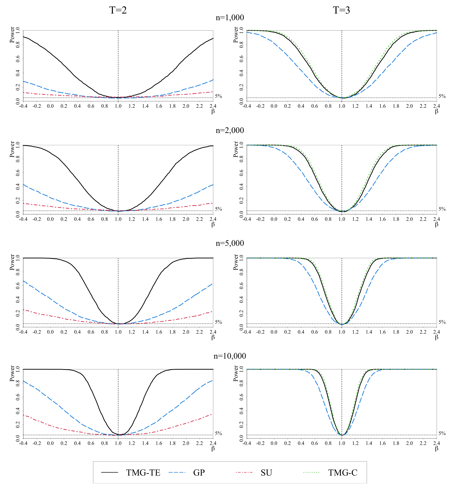
Figure S.6: Empirical power functions for TMG-TE, GP, SU and TMG-C estimators of $\beta_{0}$ $(E(\beta_{i})=\beta_{0}=1)$ in panel data models with time effects, correlated heterogeneity, $\rho_{\beta}=0.5$, and interactive effects in the $x_{it}$ equation

Notes: For details of models with time effects, where $x_{it}$ are generated as heterogeneous AR(1) processes with interactive effects, see footnote (i) to Table S.13. For the TMG-TE estimator, see footnote (ii) to Table S.8. For GP and SU estimators, see footnote (iii) to Table S.8.

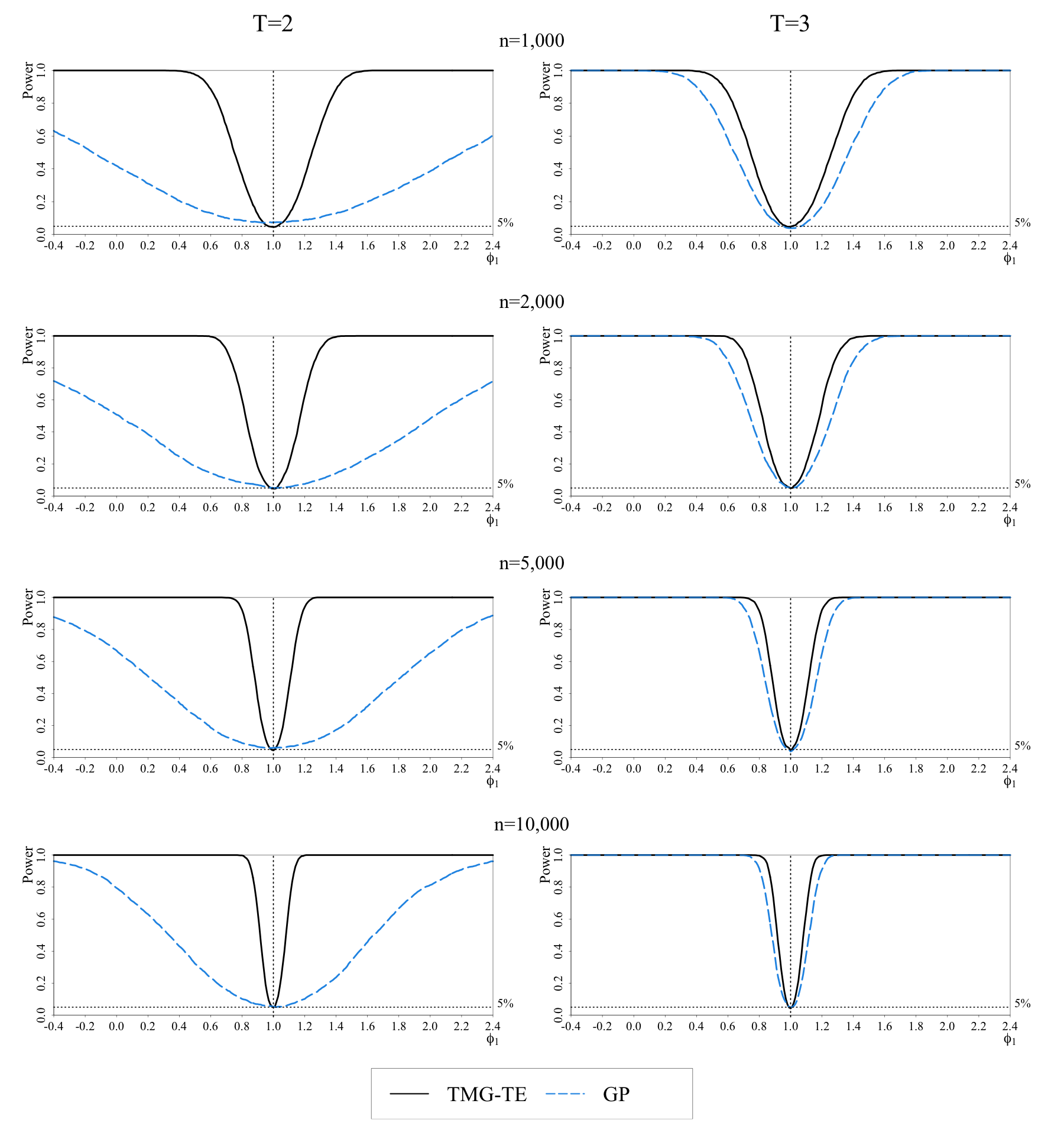
Figure S.7: Empirical power functions for TMG-TE and GP estimators of the time effect $\phi_{1}=1$ in panel data models with correlated heterogeneity, $\rho_{\beta}=0.5$, and interactive effects in the $x_{it}$ equation

Notes: For details of models with time effects, where $x_{it}$ are generated as heterogeneous AR(1) processes with interactive effects, see footnote (i) to Table S.13. For the TMG-TE estimator, see footnote (ii) to Table S.8. For the GP estimator, see footnote (iii) to Table S.8.

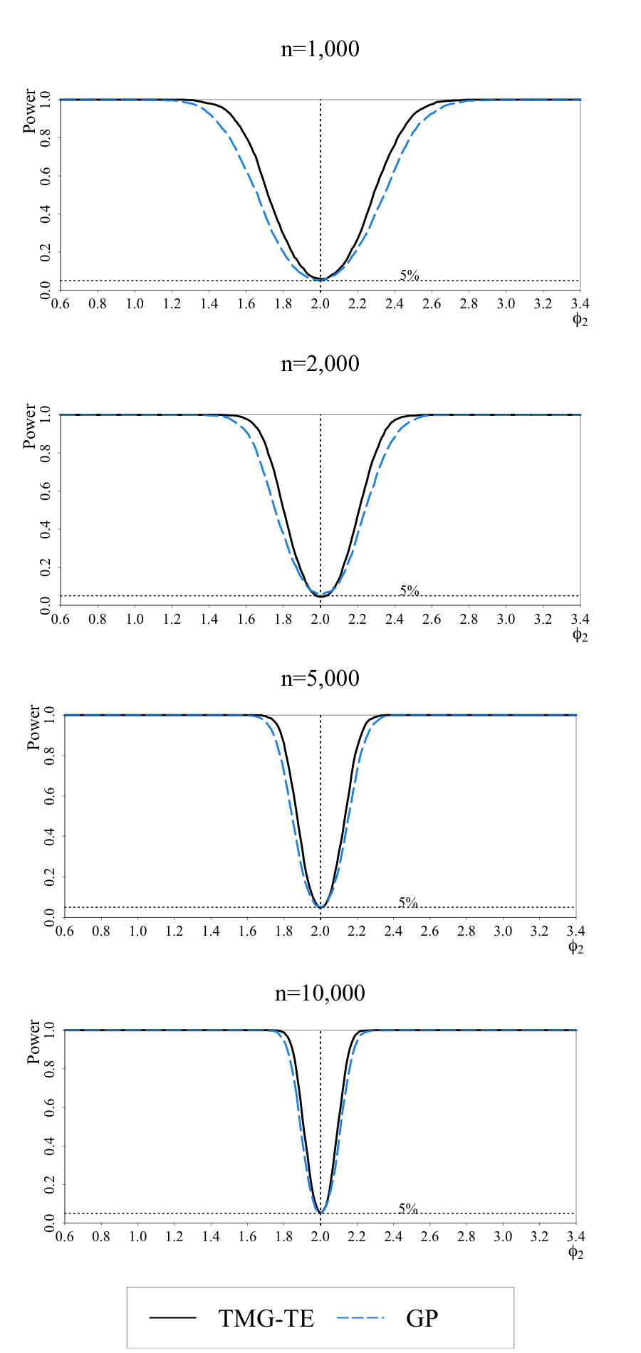
Figure S.8: Empirical power functions for TMG-TE and GP estimators of the time effect $\phi_{2}=2$ in panel data models with $T=3$, correlated heterogeneity, $\rho_{\beta}=0.5$, and interactive effects in the $x_{it}$ equation

Notes: For details of models with time effects, where $x_{it}$ are generated as heterogeneous AR(1) processes with interactive effects, see footnote (i) to Table S.13. For the TMG-TE estimator, see footnote (ii) to Table S.8. For the GP estimator, see footnote (iii) to Table S.8.

Appendix S.8 Empirical power functions for TMG-TE, TMG-C, GP and SU estimators in the baseline model with time effects and correlated heterogeneity

Figures S.9–S.11 show empirical power functions for TMG-TE, GP, SU (for $T=2$) and TMG-C (for $T=3$) estimators of $\beta_{0}$, and the time effects, $\phi_{1}$ and $\phi_{2},$ for the baseline model with correlated heterogeneity, $\rho_{\beta}=0.5$, as discussed in Section 8.2.2 of the main paper.

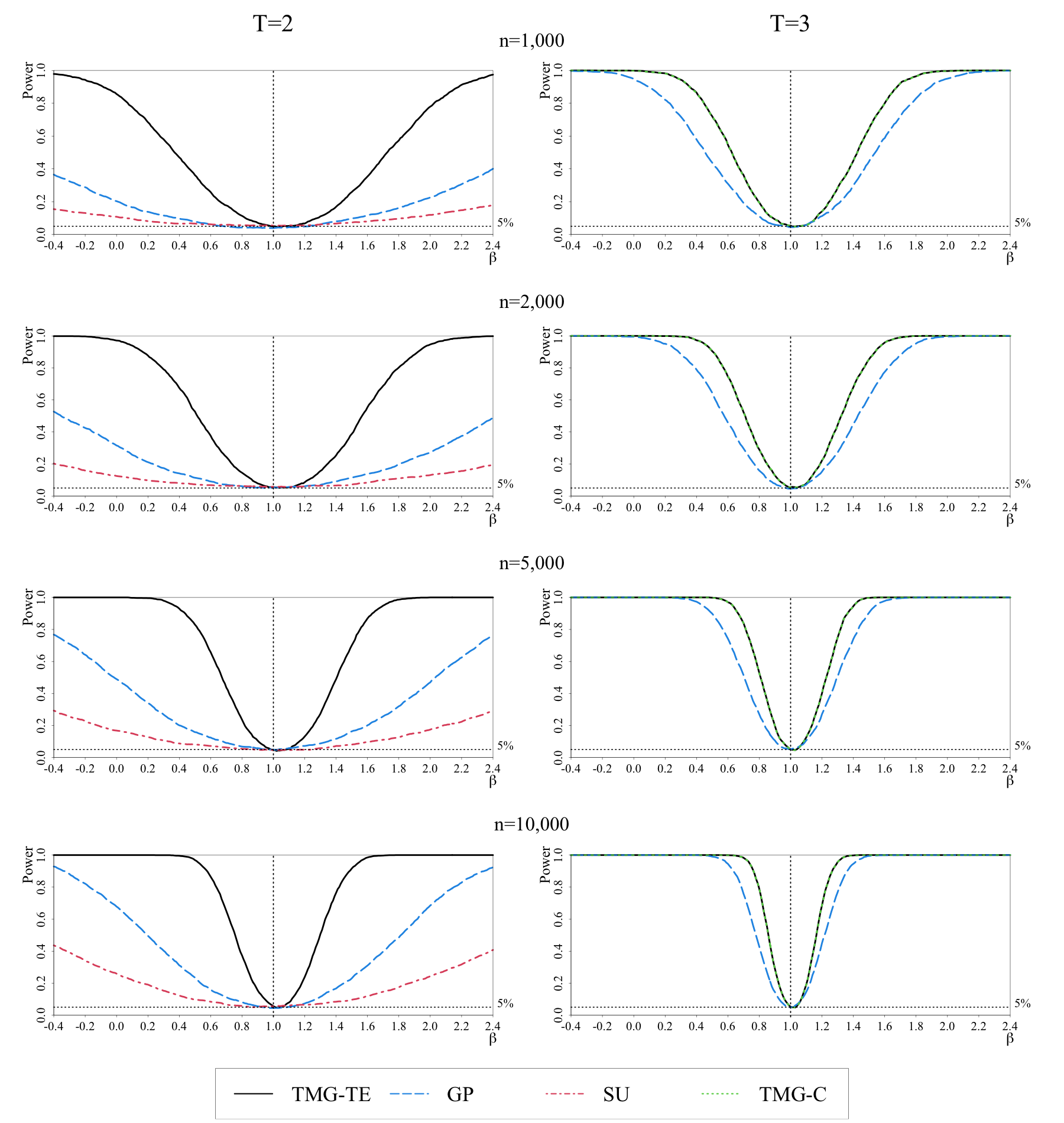
Figure S.9: Empirical power functions for TMG-TE, GP, SU and TMG-C estimators of $\beta_{0}$ $(E(\beta_{i})=\beta_{0}=1)$ in the baseline model with time effects and correlated heterogeneity, $\rho_{\beta}=0.5$

Notes: For details of the baseline model with time effects, see footnote (i) to Table 3 in the main paper.

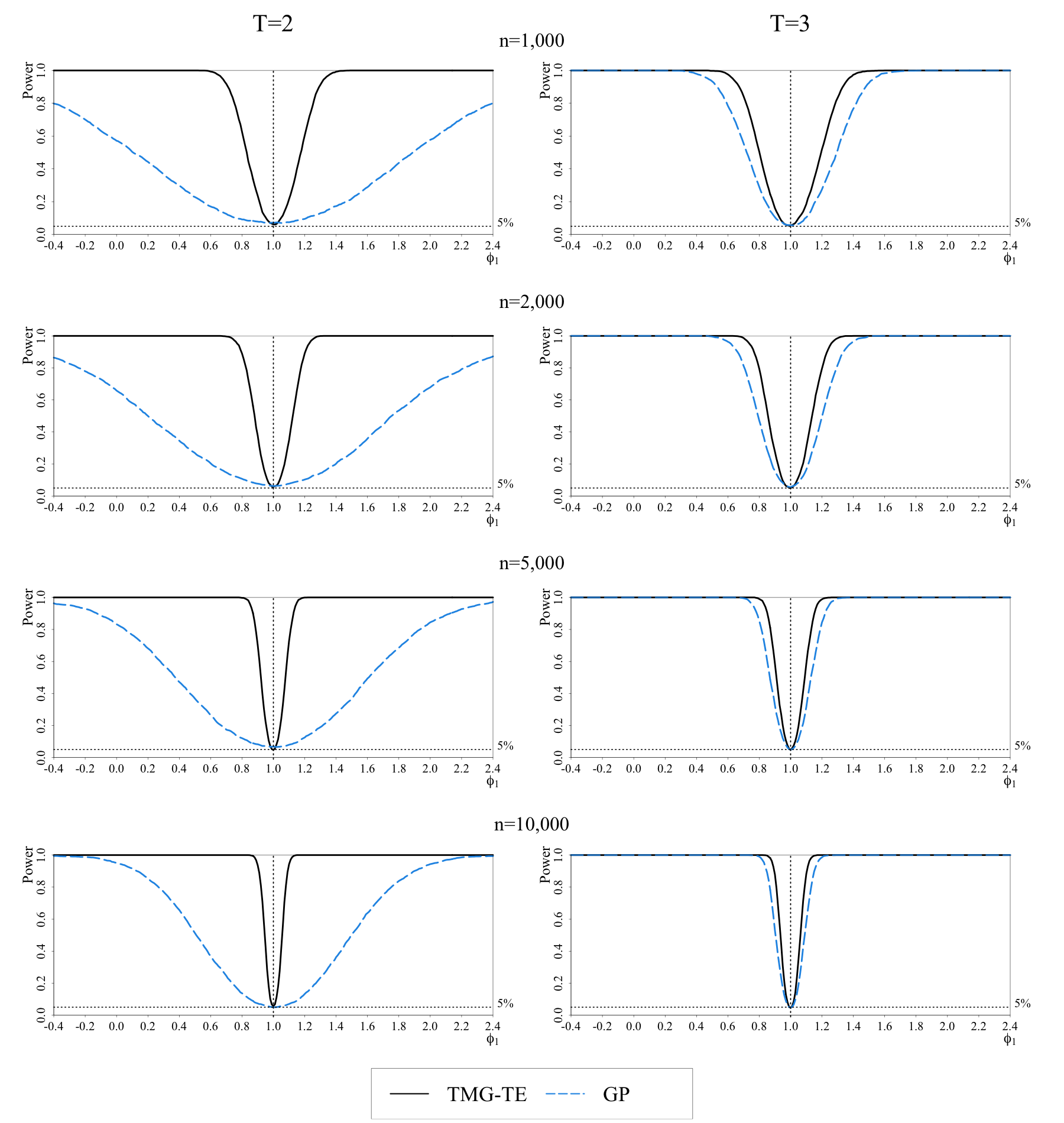
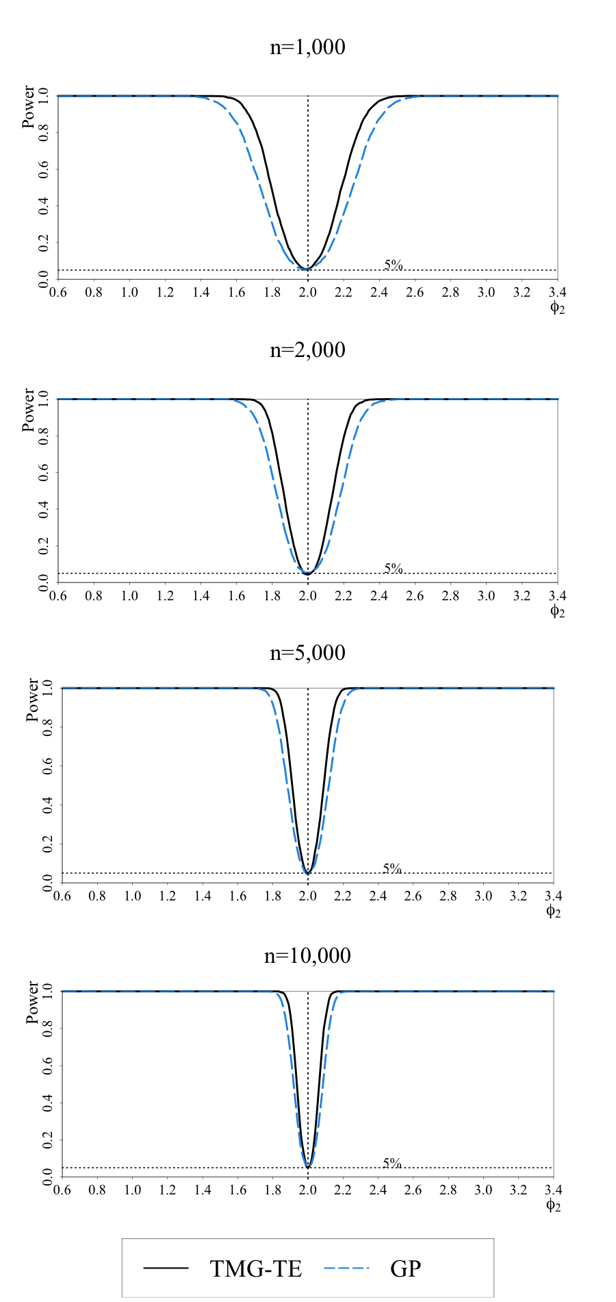
Figure S.10: Empirical power functions for TMG-TE and GP estimators of the time effect $\phi_{1}=1$ in the baseline model with correlated heterogeneity, $\rho_{\beta}=0.5$

Notes: For details of the baseline model with time effects, see footnote (i) to Table 3 in the main paper.

Figure S.11: Empirical power functions for TMG-TE and GP estimators of the time effect $\phi_{2}=2$ in the baseline model with $T=3$ and correlated heterogeneity, $\rho_{\beta}=0.5$

Notes: For details of the baseline model with time effects, see footnote (i) to Table 3 in the main paper.

Appendix S.9 Monte Carlo evidence of the Hausman-type test of correlated heterogeneity in panel data models with time effects

Table S.15: Empirical size and power of the Hausman-type test of correlated heterogeneity in the baseline model with time effects

		Under $H_{0}$										Under $H_{1}$
		Homogeneity: $\sigma_{\beta}^{2}=0$					Uncorrelated hetro.: $\rho_{\beta}=0$, $\sigma_{\beta}^{2}=0.5$					Correlated hetro.: $\rho_{\beta}=0.5$, $\sigma_{\beta}^{2}=0.5$
$T/n$		1,000	2,000	5,000	10,000		1,000	2,000	5,000	10,000		1,000	2,000	5,000	10,000
TMG-TE
2		4.3	4.4	5.3	5.5		5.7	5.4	4.9	5.9		25.0	37.1	67.0	89.5
3		4.5	5.6	5.8	4.8		5.5	4.5	5.8	4.7		39.6	59.9	90.0	99.3
4		4.9	5.7	5.6	4.9		5.0	4.2	5.5	4.7		52.1	75.5	97.3	100.0
5		5.2	4.6	4.7	5.2		4.4	4.5	4.5	4.4		61.9	84.5	99.4	100.0
6		4.7	5.2	5.5	5.3		5.2	4.3	4.6	4.4		70.4	90.9	100.0	100.0
8		5.0	4.7	5.0	5.3		4.6	4.9	5.9	5.8		79.7	95.6	100.0	100.0
TMG-C
3		4.6	5.7	5.7	4.8		5.3	4.4	5.7	4.8		39.7	59.8	89.9	99.2
4		5.0	5.6	5.7	4.9		4.9	4.5	5.5	4.7		51.9	75.6	97.3	100.0
5		5.2	4.6	4.7	5.3		4.3	4.4	4.5	4.5		62.0	84.5	99.4	100.0
6		4.8	5.2	5.5	5.3		5.2	4.3	4.7	4.5		70.8	91.0	100.0	100.0
8		4.9	4.8	5.0	5.3		4.7	5.0	5.8	5.8		80.0	95.6	100.0	100.0

Notes: (i) The baseline model for the test is generated as $y_{it}=\alpha_{i}+\phi_{t}+\beta_{i}x_{it}+u_{it}$, with $\alpha_{i}$ correlated with $x_{it}$ under both the null and alternative hypotheses. Time effects are set as $\phi_{t}=t$ for $t=1,2,...,T-1$, and $\phi_{T}=-T(T-1)/2$. The errors processes for $y_{it}$ and $x_{it}$ equations are chi-squared and Gaussian, respectively, and $x_{it}$ are generated as heterogeneous AR(1) processes. For further details see Section 8.1.3 in the main paper. (ii) The null hypothesis is given by (7.1) in the main paper, including the case of homogeneity with $\sigma_{\beta}^{2}=0$ and the case of uncorrelated heterogeneity with $\rho_{\beta}=0$ (the degree of correlated heterogeneity defined by (8.6) in the main paper) and $\sigma_{\beta}^{2}=0.5$. The alternative of correlated heterogeneity is generated with $\rho_{\beta}=0.5$ and $\sigma_{\beta}^{2}=0.5$. (iii) The test statistics for panels with time effects are based on the difference between the FE-TE and TMG-TE estimator given by (S.2.15) with $T\geq k$, and the difference between the FE-TE and TMG-C estimators given by (S.2.21) with $T>k$. For further details see Section S.2. Size and power are in per cent.

References

Pesaran, M. H. and T. Yamagata (2023). Testing for Alpha in linear factor pricing models with a large number of securities. Published online in Journal of Financial Econometrics.

Graham, B. S. and J. L. Powell (2012). Identification and estimation of average partial effects in “irregular”correlated random coefficient panel data models. Econometrica 80, 2105–2152.

Sasaki, Y. and T. Ura (2021). Slow Movers in Panel Data. arXiv preprint arXiv:2110.12041.

.

References

- Abadie and Cattaneo (2018) Abadie, A. and M. D. Cattaneo (2018). Econometric methods for program evaluation. Annual Review of Economics 10, 465–503.
- Arellano and Bonhomme (2012) Arellano, M. and S. Bonhomme (2012). Identifying distributional characteristics in random coefficients panel data models. The Review of Economic Studies 79, 987–1020.
- Athey and Imbens (2017) Athey, S. and G. W. Imbens (2017). The state of applied econometrics: causality and policy evaluation. Journal of Economic Perspectives 31, 3–32.
- Banerjee et al. (2015) Banerjee, A., D. Karlan, and J. Zinman (2015). Six randomized evaluations of microcredit: introduction and further steps. American Economic Journal: Applied Economics 7, 1–21.
- Bastagli et al. (2019) Bastagli, F., J. Hagen-Zanker, L. Harman, V. Barca, G. Sturge, and T. Schmidt (2019). The impact of cash transfers: a review of the evidence from low-and middle-income countries. Journal of Social Policy 48, 569–594.
- Bonhomme (2012) Bonhomme, S. (2012). Functional differencing. Econometrica 80, 1337–1385.
- Chamberlain (1992) Chamberlain, G. (1992). Efficiency bounds for semiparametric regression. Econometrica 60, 567–596.
- Chudik and Pesaran (2015) Chudik, A. and M. H. Pesaran (2015). Common correlated effects estimation of heterogeneous dynamic panel data models with weakly exogenous regressors. Journal of Econometrics 188, 393–420.
- Crépon and Van Den Berg (2016) Crépon, B. and G. J. Van Den Berg (2016). Active labor market policies. Annual Review of Economics 8, 521–546.
- de Chaisemartin and D’Haultfoeuille (2023) de Chaisemartin, C. and X. D’Haultfoeuille (2023). Two-way fixed effects and differences-in-differences with heterogeneous treatment effects: a survey. The Econometrics Journal 26, C1–C30.
- de Chaisemartin et al. (2023) de Chaisemartin, C., X. D’Haultfoeuille, F. Pasquier, and G. Vazquez-Bare (2023). Difference-in-differences estimators for treatments continuously distributed at every period. arXiv preprint arXiv:2201.06898.
- Graham and Powell (2012) Graham, B. S. and J. L. Powell (2012). Identification and estimation of average partial effects in “irregular” correlated random coefficient panel data models. Econometrica 80, 2105–2152.
- Heckman and Vytlacil (1998) Heckman, J. and E. Vytlacil (1998). Instrumental variables methods for the correlated random coefficient model: estimating the average rate of return to schooling when the return is correlated with schooling. Journal of Human Resources 33, 974–987.
- Lee and Sul (2022) Lee, Y. and D. Sul (2022). Trimmed mean group estimation. In Essays in Honor of M. Hashem Pesaran: Panel Modeling, Micro Applications, and Econometric Methodology. Emerald Publishing Limited.
- Pesaran and Smith (1995) Pesaran, M. H. and R. Smith (1995). Estimating long-run relationships from dynamic heterogeneous panels. Journal of Econometrics 68, 79–113.
- Pesaran et al. (1996) Pesaran, M. H., R. Smith, and K. S. Im (1996). Dynamic linear models for heterogenous panels. In P. Mátyás, Lászlóand Sevestre (Ed.), The Econometrics of Panel Data: A Handbook of the Theory with Applications. Springer Netherlands.
- Pesaran and Yamagata (2008) Pesaran, M. H. and T. Yamagata (2008). Testing slope homogeneity in large panels. Journal of Econometrics 142, 50–93.
- Pesaran and Yamagata (2023) Pesaran, M. H. and T. Yamagata (2023). Testing for Alpha in linear factor pricing models with a large number of securities. Published online in Journal of Financial Econometrics.
- Sasaki and Ura (2021) Sasaki, Y. and T. Ura (2021). Slow Movers in Panel Data. arXiv preprint arXiv:2110.12041.
- Verdier (2020) Verdier, V. (2020). Average treatment effects for stayers with correlated random coefficient models of panel data. Journal of Applied Econometrics 35, 917–939.
- Wooldridge (2005) Wooldridge, J. M. (2005). Fixed-effects and related estimators for correlated random-coefficient and treatment-effect panel data models. Review of Economics and Statistics 87, 385–390.