Solutions to the KP hierarchy with an elliptic background

Abstract

A class of “elliptic soliton” solutions of the Kadomtsev-Petviashvili hierarchy, which includes a determinantal solution of Li and Zhang, is described in terms of pseudo-differential operator formulation. In our approach, the Li-Zhang solution is obtained by repeatedly applying the Darboux transformation to a stationary solution. Real-valued solutions are discussed and various examples that display web-like patterns are presented.

1 Introduction

The relationship between soliton equations and elliptic functions is a fascinating and deep connection. An example of the connection is elliptic function solutions of the Kadomtsev-Petviashvili (KP) equation,

$$\left(4u_{t}-12uu_{x}-u_{xxx}\right)_{x}-3u_{yy}=0,$$ (1.1)

where the subscripts denote the derivatives that are being taken. The simplest elliptic solution is given by the Weierstrass $\displaystyle\wp$-function [32, 38, 41],

$$\wp(z)=\frac{1}{z^{2}}+\sum_{(m,n)\neq(0,0)}\left\{\frac{1}{\left(z+2m\omega_{1}+2n\omega_{2}\right)^{2}}-\frac{1}{\left(2m\omega_{1}+2n\omega_{2}\right)^{2}}\right\},$$ (1.2)

where $\displaystyle\omega_{1}$, $\displaystyle\omega_{2}$ is a fundamental pair of half-periods: $\displaystyle\wp(z+2\omega_{i})=\wp(z)$ ($\displaystyle i=1,2$). It is well-known that (1.2) satisfies the following differential equations:

$$\displaystyle\left\{\frac{d\wp(x)}{dx}\right\}^{2} \displaystyle=4\wp(x)^{3}-g_{2}\wp(x)-g_{3},$$ (1.3)

$$\displaystyle\frac{d^{2}\wp(x)}{dx^{2}} \displaystyle=6\wp(x)^{2}-\frac{g_{2}}{2},$$ (1.4)

where the constants $\displaystyle g_{2}$, $\displaystyle g_{3}$ are given by

$$g_{2}=60\sum_{(m,n)\neq(0,0)}\frac{1}{\left(2m\omega_{1}+2n\omega_{2}\right)^{4}},\quad g_{3}=140\sum_{(m,n)\neq(0,0)}\frac{1}{\left(2m\omega_{1}+2n\omega_{2}\right)^{6}}.$$ (1.5)

It is clear from (1.4) that

$$u(x,y,t)=-\wp\left(x\right)$$ (1.6)

is a stationary solution to the KP equation (1.1). A non-stationary solution can be attained through the application of a Galilean-type transformation:

$$u(x,y,t)=-\wp\left(x+2ay+3a^{2}t\right)$$ (1.7)

where $\displaystyle a$ is an arbitrary constant.

Recently, Li and Zhang [17, 18] obtained Wronskian representation for a class of “elliptic soliton” solutions to the Korteweg-de Vries (KdV) equation,

$$4u_{t}=12uu_{x}+u_{xxx},$$ (1.8)

and for the KP equation (1.1). The elements of Wronskians are a composition of Lamé-type plane wave factors,

$$\Phi(x;k)=\frac{\sigma(x+k)}{\sigma(x)}e^{-\zeta(k)x},$$ (1.9)

where $\displaystyle k$ is a constant. Here we have used the Weierstrass functions $\displaystyle\zeta$ and $\displaystyle\sigma$ that are related to $\displaystyle\wp$ as follows:

$$\wp(x)=-\frac{d\zeta(x)}{dx},\quad\zeta(x)=\frac{1}{\sigma(x)}\cdot\frac{d\sigma(x)}{dx}.$$ (1.10)

Note that (1.9) is slightly different from the plane wave factor used in [17, 18] (up to multiplication of $\displaystyle\sigma(k)$).

We remark that the term “elliptic solitons” is used in various ways. In [17, 18], as mentioned above, the solutions are constructed by the Weierstrass functions $\displaystyle\wp$, $\displaystyle\zeta$ and $\displaystyle\sigma$ and Li and Zhang call their solutions as “elliptic solitons” after [27, 42]. On the other hand, in [15, 37, 40], the term “elliptic solitons” refers to algebro-geometric solutions of soliton equations that exhibit doubly-periodic behavior in one variable, while $\displaystyle\Phi(x;k)$ (1.9) is quasi-periodic in $\displaystyle x$:

$$\Phi(x+2\omega_{j};k)=e^{2\left\{\zeta(\omega_{j})k-\zeta(k)\omega_{j}\right\}}\Phi(x;k)\quad(j=1,2).$$ (1.11)

In this paper, we investigate “elliptic solitons” in former sense. In [17, 18], Li and Zhang studied a function $\displaystyle f$ of the form,

$$\displaystyle f \displaystyle=\mathcal{W}\left(\varphi_{1},\ldots,\varphi_{n}\right),$$ (1.12)

$$\displaystyle\varphi_{j} \displaystyle=a_{j}^{+}\Phi(x;k_{j})e^{-\gamma(k_{j})}+a_{j}^{-}\Phi(x;-k_{j})e^{\gamma(k_{j})}\quad(j=1,\ldots,n),$$

$$\displaystyle\gamma(k) \displaystyle=\wp(k)y-\frac{\wp^{\prime}(k)}{2}t\quad\left(\wp^{\prime}(x)=\frac{d\wp(x)}{dx}\right),$$

where $\displaystyle\mathcal{W}\left(\varphi_{1},\ldots,\varphi_{n}\right)$ denotes the Wronskian determinant, and proved that (1.12) satisfies a Hirota-type bilinear differential equation,

$$\left(D_{x}^{4}-4D_{x}D_{t}-12\wp(x)D_{x}^{2}+3D_{y}^{2}\right)f\cdot f=0.$$ (1.13)

Here $\displaystyle D_{x}$, $\displaystyle D_{y}$, $\displaystyle D_{t}$ are Hirota’s bilinear operators:

$$\displaystyle D_{x}^{l}D_{y}^{m}D_{t}^{n}f\cdot g$$

$$\displaystyle=\left.\left(\frac{\partial}{\partial x}-\frac{\partial}{\partial x^{\prime}}\right)^{l}\left(\frac{\partial}{\partial y}-\frac{\partial}{\partial y^{\prime}}\right)^{m}\left(\frac{\partial}{\partial t}-\frac{\partial}{\partial t^{\prime}}\right)^{n}f(x,y,t)g(x^{\prime},y^{\prime},t^{\prime})\right|_{x^{\prime}=x,y^{\prime}=y,t^{\prime}=t}.$$ (1.14)

Although the bilinear equation (1.13) contains the $\displaystyle\wp$-function in the coefficient, it can be shown that

$$u=-\wp(x)+\left(\log f\right)_{xx}$$ (1.15)

satisfies the KP equation (1.1) without $\displaystyle\wp$-function coefficient. In other words, $\displaystyle u$ of (1.15) represents a solution of the KP equation with the $\displaystyle\wp$-function background. In the case of the KdV equation, solutions of this class has been discussed in [16] based on the approach of Shabat [36]. We remark that solutions of nonlinear Schrödinger type equations with elliptic backgrounds have been studied as a model for density-modulated quantum condensates in [39], and as a model for rogue waves in [3, 7].

The principal aim of this paper is to investigate hierarchy structure that includes the solution (1.15). Li and Zhang [17, 18] introduced higher order time variables $\displaystyle t_{2},t_{3},\ldots$ and studied hierarchy structure associated with the Wronskian solutions (1.12). They obtained an infinite sequence of Hirota-type bilinear equations such as

$$\displaystyle\left(D_{x}^{4}-4D_{x}D_{t_{3}}+3D_{t_{2}}^{2}-g_{2}\right)\tilde{f}\cdot\tilde{f}=0,$$ (1.16)

$$\displaystyle\left(D_{x}^{3}D_{t_{2}}+2D_{t_{2}}D_{t_{3}}-3D_{x}D_{t_{4}}\right)\tilde{f}\cdot\tilde{f}=0,$$ (1.17)

$$\displaystyle\left(D_{x}^{6}-20D_{x}^{3}D_{t_{3}}-80D_{t_{3}}^{2}+144D_{x}D_{t_{5}}-45D_{x}^{2}D_{t_{2}}^{2}+3g_{2}D_{x}^{2}-24g_{3}\right)\tilde{f}\cdot\tilde{f}=0,$$ (1.18)

$$\displaystyle\left(D_{x}^{6}+4D_{x}^{3}D_{t_{3}}-32D_{t_{3}}^{2}-9D_{x}^{2}D_{t_{2}}^{2}+36D_{t_{2}}E_{t_{4}}+3g_{2}D_{x}^{2}-24g_{3}\right)\tilde{f}\cdot\tilde{f}=0,$$ (1.19)

$$\displaystyle\qquad\vdots$$

As mentioned in [18], (1.16) is transformed to (1.13) by setting $\displaystyle\tilde{f}=\sigma(x)f$. Li and Zhang proposed a generating function of bilinear equations (bilinear identity) that includes (1.16)–(1.19) using vertex operators [18].

If we set $\displaystyle g_{2}=g_{3}=0$, the bilinear equations (1.16)–(1.19) coincide with those of the KP hierarchy listed in [13]. On the other hand, if we set

$$\tilde{f}=\exp\left[\frac{g_{2}}{4}\left\{(1+2a)t_{2}^{2}+(1+3a)xt_{3}\right\}\right]\tau$$ (1.20)

for $\displaystyle a$ is an arbitrary constant, then $\displaystyle\tau$ satisfies

$$\left(D_{x}^{4}-4D_{x}D_{t_{3}}+3D_{t_{2}}^{2}\right)\tau\cdot\tau=0,$$ (1.21)

which is the bilinear form of the original KP equation (1.1). This suggests that the bilinear equations with elliptic solitons may be transformed to the equations without elliptic parameters $\displaystyle g_{2}$, $\displaystyle g_{3}$ via suitable transformation like (1.20). We will show that bilinear equations associated with the Li-Zhang solution (1.12) are actually equivalent to those of the original KP hierarchy without elliptic parameters $\displaystyle g_{2}$, $\displaystyle g_{3}$. We will construct the transformation from the Li-Zhang solution (1.12) to a $\displaystyle\tau$-function of the KP hierarchy via pseudo-differential operator formulation.

It should be remarked that solutions with the $\displaystyle\wp$-function background has been discussed in [25, 26] as certain degeneration of hyperelliptic solutions, using the correspondence between algebro-geometric solutions and the Sato Grassmannian. We also remark that a similar results can be found in [11]. The approach for handling elliptic solitons in this paper doesn’t rely on the algebro-geometric framework. Instead, we employ a formulation based on pseudo-differential operators and utilize elementary properties of the Weierstrass functions $\displaystyle\wp$, $\displaystyle\zeta$ and $\displaystyle\sigma$.

2 Pseudo-differential operators and KP hierarchy

The KP hierarchy is an infinite (countable) family of partial differential equations that includes the KP equation (1.1). Here we give a brief review of the KP hierarchy using pseudo-differential operator formulation [5, 31, 33, 34, 35].

2.1 Pseudo-differential operators

Let $\displaystyle\mathcal{A}$ be an associative ring and $\displaystyle\partial_{x}:\mathcal{A}\to\mathcal{A}$ its derivation. Let us consider the ring of formal pseudo-differential operators:

$$\mathcal{E}=\left\{\sum_{-\infty<n\ll+\infty}a_{n}\partial_{x}^{n},\;a_{n}\in\mathcal{A}\right\}.$$ (2.1)

Multiplication can be defined according to the generalized Leibniz rule:

$$\left(\sum_{n}a_{n}\partial_{x}^{n}\right)\left(\sum_{m}b_{m}\partial_{x}^{m}\right)=\sum_{n,m}a_{i}\sum_{r=0}^{\infty}\binom{n}{r}\partial_{x}^{r}(b_{m})\partial_{x}^{n+m-r}.$$ (2.2)

Here the generalized binomial coefficient is defined by

$$\binom{n}{r}=\begin{cases}1&(r=0),\\ \frac{n(n-1)\cdots(n-r+1)}{r!}&(r\neq 0).\end{cases}$$ (2.3)

For $\displaystyle P=\sum_{-\infty<n\leq m}a_{n}\partial_{x}^{n}\in\mathcal{E}$ ($\displaystyle a_{m}\neq 0$), denote by $\displaystyle\mathrm{ord}_{\partial_{x}}(P)=m$ the leading order of $\displaystyle P$. Let $\displaystyle\mathcal{E}^{(m)}$ be a subspace of $\displaystyle\mathcal{E}$ with the following property:

$$\mathcal{E}^{(m)}=\left\{P\in\mathcal{E}\;|\;\mathrm{ord}_{\partial_{x}}(P)\leq m\right\},$$ (2.4)

and let $\displaystyle\mathcal{D}$ be a subring of differential operators:

$$\mathcal{D}=\left\{\sum_{0\leq n\ll+\infty}a_{n}\partial_{x}^{n},\;a_{n}\in\mathcal{A}\right\}.$$ (2.5)

Then $\displaystyle\mathcal{E}$ has a natural decomposition $\displaystyle\mathcal{E}=\mathcal{D}\oplus\mathcal{E}^{(-1)}$. Denote by $\displaystyle(\,\cdot\,)_{\geq 0}$ the projection to $\displaystyle\mathcal{D}$, and by $\displaystyle(\,\cdot\,)_{<0}$ the projection to $\displaystyle\mathcal{E}^{(-1)}$, i.e., for $\displaystyle m>0$,

$$\displaystyle\left(\sum_{-\infty<n\leq m}a_{n}\partial_{x}^{n}\right)_{\geq 0} \displaystyle=\sum_{0\leq n\leq m}a_{n}\partial_{x}^{n}\in\mathcal{D},$$ (2.6)

$$\displaystyle\left(\sum_{-\infty<n\leq m}a_{n}\partial_{x}^{n}\right)_{<0} \displaystyle=\sum_{-\infty<n<0}a_{n}\partial_{x}^{n}\in\mathcal{E}^{(-1)}.$$ (2.7)

We prepare several formulas that we shall use later.

Lemma 2.1 (Helminck and van de Leur [9, 10] (cf. Oevel [28], (2.10))).

Let $\displaystyle a,b\in\mathcal{A}$, $\displaystyle P=\sum_{j=-\infty}^{m}p_{j}\partial^{j}\in\mathcal{E}$, and $\displaystyle\mathrm{Res}_{\partial_{x}}(P)=p_{-1}$. Then the following relations hold:

$$\displaystyle(aPb)_{\geq 0}=a(P)_{\geq 0}b,\quad(aPb)_{<0}=a(P)_{<0}b,$$ (2.8)

$$\displaystyle\mathrm{Res}_{\partial_{x}}(aPb)=ab\,\mathrm{Res}_{\partial_{x}}(P),$$ (2.9)

$$\displaystyle\left(\partial_{x}P\right)_{<0}=\partial_{x}(P)_{<0}-\mathrm{Res}_{\partial_{x}}(P),$$ (2.10)

$$\displaystyle\left(P\partial_{x}\right)_{<0}=(P)_{<0}\partial_{x}-\mathrm{Res}_{\partial_{x}}(P),$$ (2.11)

$$\displaystyle\left(P\partial_{x}^{-1}\right)_{<0}=(P)_{<0}\partial_{x}^{-1}+\mathrm{Res}_{\partial_{x}}(P\partial_{x}^{-1})\partial_{x}^{-1},$$ (2.12)

$$\displaystyle\mathrm{Res}_{\partial_{x}}\left(Pa\partial^{-1}\right)=(P)_{\geq 0}(a),$$ (2.13)

where the right-hand-side of (2.13) means that the differential operator $\displaystyle(P)_{\geq 0}$ acts on $\displaystyle a\in\mathcal{A}$.

2.2 KP hierarchy

We introduce an infinite set of “time” variables $\displaystyle\bm{t}=\left(t_{2},t_{3},\ldots\right)$. Usually $\displaystyle x$ is identified as $\displaystyle t_{1}$, but we do not follow this convention to distinguish between $\displaystyle x$ and the time variables $\displaystyle\bm{t}=\left(t_{2},t_{3},\ldots\right)$, except for Lemma 4.6. We consider generalized Lax operator $\displaystyle L$ of the form

$$L=\partial_{x}+\sum_{j=1}^{\infty}u_{j+1}\partial_{x}^{-j},\quad u_{j+1}=u_{j+1}(x,\bm{t}),$$ (2.14)

We say that a Lax operator $\displaystyle L$ is a solution to the KP hierarchy if and only if it satisfies the generalized Lax equations:

$$\frac{\partial L}{\partial t_{n}}=\left[B_{n},\,L\right],\quad B_{n}=\left(L^{n}\right)_{\geq 0}\quad(n=2,3,\ldots).$$ (2.15)

The explicit forms of $\displaystyle B_{2}$, $\displaystyle B_{3}$ are given by

$$B_{2}=\partial_{x}^{2}+2u_{2},\quad B_{3}=\partial_{x}^{3}+3u_{2}+3u_{3}+3\frac{\partial u_{2}}{\partial x}.$$ (2.16)

The Lax equations (2.15) are equivalent to the following infinite set of equations (Zakharov-Shabat equations):

$$\frac{\partial B_{m}}{\partial t_{n}}-\frac{\partial B_{n}}{\partial t_{m}}=\left[B_{n},B_{m}\right]\quad(m,n=2,3,\ldots).$$ (2.17)

Applying (2.16) to (2.17) with $\displaystyle m=2$, $\displaystyle n=3$, one can show that $\displaystyle u=u_{2}(x,t_{2},t_{3})$ satisfies the KP equation (1.1) ($\displaystyle y=t_{2}$, $\displaystyle t=t_{3}$).

The equations (2.15) and (2.17) are compatibility conditions for the following auxiliary linear problem:

$$\displaystyle L\psi \displaystyle=\lambda\psi,\quad\psi=\psi(x,\bm{t};\lambda),$$ (2.18)

$$\displaystyle\frac{\partial\psi}{\partial t_{n}} \displaystyle=B_{n}\psi\quad(n=1,2,\ldots).$$ (2.19)

Let us consider a solution of (2.18) and (2.19) of the form

$$\psi(x,\bm{t};\lambda) =\hat{w}(x,\bm{t};\lambda)e^{\xi(x,\bm{t};\lambda)},$$ (2.20)

$$\hat{w}(x,\bm{t};\lambda) =1+\sum_{j=1}^{\infty}w_{j}(x,\bm{t})\lambda^{-j},$$

$$\xi(x,\bm{t};\lambda) =\lambda x+\sum_{j=2}^{\infty}\lambda^{j}t_{j}.$$

The function $\displaystyle\psi$ of the form (2.20) is called the wave function (or the formal Baker-Akhiezer function) associated with $\displaystyle L$.

Define a space $\displaystyle M$ as [10]

$$M=\left\{\left(\sum_{-\infty<j\ll+\infty}a_{j}z^{j}\right)e^{\xi(x,\bm{t};\lambda)}\;\Bigg{|}\;a_{j}\in\mathcal{A}\right\},$$ (2.21)

which is an $\displaystyle\mathcal{E}$-module:

$$\displaystyle b \displaystyle\left\{\left(\sum_{-\infty<j\ll+\infty}a_{j}z^{n}\right)e^{\xi(x,\bm{t};\lambda)}\right\}=\left(\sum_{-\infty<j\ll+\infty}ba_{j}z^{n}\right)e^{\xi(x,\bm{t};\lambda)}\quad(b\in\mathcal{A}),$$

$$\displaystyle\partial_{x} \displaystyle\left\{\left(\sum_{-\infty<j\ll+\infty}a_{j}z^{n}\right)e^{\xi(x,\bm{t};\lambda)}\right\}=\left\{\sum_{j}\partial_{x}(a_{j})z^{n}+\sum_{j}a_{j}z^{j+1}\right\}e^{\xi(x,\bm{t};\lambda)},$$ (2.22)

$$\displaystyle\frac{\partial}{\partial t_{n}} \displaystyle\left\{\left(\sum_{-\infty<j\ll+\infty}a_{j}z^{n}\right)e^{\xi(x,\bm{t};\lambda)}\right\}=\left(\sum_{j}\frac{\partial a_{j}}{\partial t_{n}}z^{n}+\sum_{j}a_{j}z^{j+n}\right)e^{\xi(x,\bm{t};\lambda)}.$$

Using (2.22), one can introduce $\displaystyle W\in\mathcal{E}^{(0)}$ as

$$W=1+\sum_{j=1}^{\infty}w_{j}(x,\bm{t})\partial_{x}^{-j}$$ (2.23)

which is called the wave operator or the dressing operator. From (2.18) and (2.19), we have

$$\displaystyle\psi(x,\bm{t};\lambda)=We^{\xi(x,\bm{t};\lambda)},\quad L=W\partial_{x}W^{-1},$$ (2.24)

$$\displaystyle\frac{\partial W}{\partial t_{n}}=B_{n}W-W\partial_{x}^{n}=-\left(W\partial_{x}^{n}W^{-1}\right)_{<0}W.$$ (2.25)

The equation (2.25) is called the Sato-Wilson equation. We remark that the coefficients of $\displaystyle L$ can be written in terms of $\displaystyle w_{j}$ ($\displaystyle j=1,2,\ldots$):

$$u_{2} =-w^{\prime}_{1},\quad u_{3}=-w^{\prime}_{2}+w_{1}w^{\prime}_{1},$$ (2.26)

$$u_{4} =-w^{\prime}_{3}+w_{1}w^{\prime}_{2}+w^{\prime}_{1}w_{2}-w_{1}^{2}w^{\prime}_{1}-\left(w^{\prime}_{1}\right)^{2},\ldots.$$

Here and hereafter, the prime denotes differentiation with respect to $\displaystyle x$.

Theorem 2.2 (Existence of $\displaystyle\tau$-function [5]).

If $\displaystyle\psi(x,\bm{t};\lambda)$ is a wave function (or a formal Baker-Akhiezer function) of the KP hierarchy, then there exists a function $\displaystyle\tau(x,\bm{t})$ ($\displaystyle\tau$-funcion) that is related to $\displaystyle\hat{w}(x,\bm{t};\lambda)$ of (2.20) as

$$\hat{w}(x,\bm{t};\lambda)=\frac{\tau\left(x-\lambda^{-1},\bm{t}-\left[\lambda^{-1}\right]\right)}{\tau(x,\bm{t})},$$ (2.27)

where

$$\bm{t}-\left[\lambda^{-1}\right]=\left(t_{2}-\frac{1}{2\lambda^{2}},\,t_{3}-\frac{1}{3\lambda^{3}},\,\ldots,\,t_{n}-\frac{1}{n\lambda^{n}},\,\ldots\right).$$ (2.28)

Expanding (2.27) with respect to $\displaystyle\lambda^{-1}$, one obtains (cf. [31])

$$w_{1} =-\frac{1}{\tau}\frac{\partial\tau}{\partial x},\quad w_{2}=\frac{1}{2\tau}\left(\frac{\partial^{2}\tau}{\partial x^{2}}-\frac{\partial\tau}{\partial t_{2}}\right),$$ (2.29)

$$w_{3} =-\frac{1}{6\tau}\left(\frac{\partial^{3}\tau}{\partial x^{3}}-3\frac{\partial^{2}\tau}{\partial x\partial t_{2}}+2\frac{\partial\tau}{\partial t_{3}}\right),\;\ldots.$$

Applying these relations to (2.26), we obtain (cf. [31])

$$u_{2} =\frac{\partial^{2}}{\partial x^{2}}\log\tau,\quad u_{3}=\frac{1}{2}\left(-\frac{\partial^{3}}{\partial x^{3}}+\frac{\partial^{2}}{\partial x\partial t_{2}}\right)\log\tau,$$ (2.30)

$$u_{4} =\frac{1}{6}\left(\frac{\partial^{4}}{\partial x^{4}}-3\frac{\partial^{3}}{\partial x^{2}\partial t_{2}}+2\frac{\partial^{2}}{\partial x\partial t_{3}}\right)\log\tau-\left(\frac{\partial^{2}}{\partial x^{2}}\log\tau\right)^{2},\;\ldots.$$

Theorem 2.3 (Bilinear identity [5, 13, 23]).

If $\displaystyle\tau(x,\bm{t})$ is a $\displaystyle\tau$-function of the KP hierarchy, then $\displaystyle\tau(x,\bm{t})$ satisfies the following equation (bilinear identity) for any $\displaystyle x$, $\displaystyle x^{\prime}$, $\displaystyle\bm{t}$ and $\displaystyle\bm{t}^{\prime}$:

$$\mathrm{Res}_{\lambda}\left[e^{\xi(x-x^{\prime},\bm{t}-\bm{t}^{\prime};\lambda)}\tau\left(x-\lambda^{-1},\,\bm{t}-\left[\lambda^{-1}\right]\right)\tau\left(x^{\prime}+\lambda^{-1},\,\bm{t}^{\prime}+\left[\lambda^{-1}\right]\right)\right]=0,$$ (2.31)

where $\displaystyle\mathrm{Res}_{\lambda}$ is the formal residue: $\displaystyle\mathrm{Res}_{\lambda}\left[\sum_{n}a_{n}\lambda^{n}\right]=a_{-1}$. Conversely, if $\displaystyle\tau(x,\bm{t})$ satisfies the bilinear identity (2.31), then the corresponding $\displaystyle\psi(x,\bm{t})$ via the formulas (2.20) and (2.27) solves the auxiliary linear problem (2.18), (2.19).

2.3 Galilean symmetry of the KP hierarchy

The Galilean-type transformation used in (1.7) can be generalized to the whole KP hierarchy. For $\displaystyle\bm{t}=\left(t_{2},t_{3},\ldots\right)$, define $\displaystyle T(\bm{t})$ as

$$T\left(x,\bm{t}\right)=\left(x+\sum_{j=2}^{\infty}\binom{j}{1}a^{j-1}t_{j},\,\sum_{j=2}^{\infty}\binom{j}{2}a^{j-2}t_{j},\,\ldots,\,\sum_{j=n}^{\infty}\binom{j}{n}a^{j-n}t_{j},\,\ldots\right).$$ (2.32)

Theorem 2.4 (Galilean symmetry of the KP hierarchy).

Let $\displaystyle L(x,\bm{t})\in\mathcal{E}^{(1)}$ of the form (2.14) be a solution of the KP hierarchy. Define $\displaystyle\tilde{L}(x,\bm{t})$ as

$$\tilde{L}(x,\bm{t})=e^{ax}L(x,\bm{t})e^{-ax}+a$$ (2.33)

for $\displaystyle a$ is an constant. Then $\displaystyle\tilde{L}\left(x,T(\bm{t})\right)$ is also of the form (2.14) and satisfies the KP hierarchy.

Proof.

It follows from (2.8) that

$$\displaystyle\left(\tilde{L}^{m}\right)_{\geq 0} \displaystyle=\sum_{n=0}^{m}\binom{m}{n}a^{m-n}e^{ax}\left(L^{n}\right)_{\geq 0}e^{-ax}.$$ (2.34)

We introduce a new set of time-variables $\displaystyle\tilde{\bm{t}}=\left(\tilde{t}_{1},\tilde{t}_{2},\ldots\right)$ and define $\displaystyle\bm{t}=T\left(\tilde{\bm{t}}\right)$, i.e.,

$$t_{n}=\sum_{j=n}^{\infty}\binom{j}{n}a^{j-n}\tilde{t}_{j}\quad(n=1,2,\ldots).$$ (2.35)

Using (2.34), we have

$$\displaystyle\frac{\partial}{\partial\tilde{t}_{m}} \displaystyle\tilde{L}\left(T(\tilde{x},\tilde{\bm{t}})\right)=\sum_{n=1}^{m}\binom{m}{n}a^{m-n}e^{ax}\frac{\partial L\left(x,\bm{t}\right)}{\partial t_{n}}e^{-ax}$$

$$\displaystyle=\sum_{n=0}^{m}\binom{m}{n}a^{m-n}\left[e^{ax}\left(L^{n}\right)_{\geq 0}e^{-ax},\,e^{ax}Le^{-ax}\right]=\left[\left(\tilde{L}^{m}\right)_{\geq 0},\,\tilde{L}\right],$$ (2.36)

which proves the desired result. ∎

Corollary 2.5 (Galilean symmetry of the KP equation).

Let $\displaystyle u(x,y,t)$ be a solution of the KP equation (1.1). Then $\displaystyle\tilde{u}(x,y,t)=u(x+2ay+3a^{2}t,y+3at,t)$ is also a solution with arbitrary constant $\displaystyle a$.

2.4 Darboux transformation for the KP hierarchy

Let $\displaystyle L\in\mathcal{E}^{(1)}$ of the form (2.14) be a solution of the KP hierarchy, and $\displaystyle\psi$ an associated wave function of the form (2.20). In this subsection, we consider a kind of gauge transformation

$$L\mapsto\tilde{L}=\mathrm{Ad}_{G}(L)=GLG^{-1},\quad\psi\mapsto\tilde{\psi}=G\psi,$$ (2.37)

where $\displaystyle G\in\mathcal{E}$ is an invertible pseudo-differential operator. If $\displaystyle\tilde{L}$ is again another solution of the KP hierarchy and $\displaystyle\tilde{\psi}$ is the wave function associated to $\displaystyle\tilde{L}$, we call the transformation (2.37) a Darbourx transformation. Darboux transformations for the KP hierarchy have been discussed by many authors [2, 8, 9, 10, 19, 28, 29, 30]. Among those, hereafter we shall follow the pseudo-differential operator formulation by Helminck and van de Leur [8, 9, 10] (cf. [30]).

Theorem 2.6 (Elementary Darboux transformation for the KP hierarchy [8, 9, 10, 30]).

Let $\displaystyle W\in\mathcal{E}^{(0)}$ be a monic pseudo-differential operator that satisfies the Sato-Wilson equation (2.25). Let $\displaystyle\varphi(x,\bm{t})$ satisfy

$$\frac{\partial\varphi(x,\bm{t})}{\partial t_{n}}=B_{n}\varphi(x,\bm{t}),\quad B_{n}=\left(W\partial_{x}^{n}W^{-1}\right)_{\geq 0}.$$ (2.38)

We say $\displaystyle\varphi(x,\bm{t})$ is an eigenfunction of the Lax operator $\displaystyle L=W\partial_{x}W^{-1}$ if it satisfies (2.38).

Define a first order differential operator $\displaystyle G_{\varphi}$ as

$$G_{\varphi}=\varphi\partial_{x}\varphi^{-1}=\partial_{x}-\frac{\varphi^{\prime}}{\varphi}=\partial_{x}-\left(\log\varphi\right)^{\prime},$$ (2.39)

which satisfies

$$\displaystyle G_{\varphi}\left(\varphi\right) \displaystyle=0,$$ (2.40)

$$\displaystyle\partial_{n}\left(G_{\varphi}\right) \displaystyle=-\partial_{n}\partial_{x}\left(\log\varphi\right)=-\left[\partial_{x},\partial_{n}\left(\log\varphi\right)\right]=-\left[G_{\varphi},\partial_{n}\left(\log\varphi\right)\right].$$ (2.41)

Using $\displaystyle G_{\varphi}$, we define another monic pseudo-differential operator $\displaystyle W_{\varphi}\in\mathcal{E}^{(0)}$ as

$$W_{\varphi}=G_{\varphi}W\partial_{x}^{-1}.$$ (2.42)

Then $\displaystyle W_{\varphi}$ also solves the Sato-Wilson equation (2.25).

A proof of Theorem 2.6 can be found in [8] (Proposition 4.1).

Theorem 2.7 (Darboux transformation in terms of $\displaystyle\tau$-functions [8, 9, 10]).

Denote by $\displaystyle\tau(x,\bm{t})$ (resp. $\displaystyle\tau_{\varphi}(x,\bm{t})$) the $\displaystyle\tau$-function corresponds to $\displaystyle W$ (resp. $\displaystyle W_{\varphi}$). Then $\displaystyle\tau_{\varphi}(x,\bm{t})$ can be written as

$$\tau_{\varphi}(x,\bm{t})=\varphi(x,\bm{t})\tau(x,\bm{t}).$$ (2.43)

A proof of Theorem 2.7 can be found in [9, 10].

Lemma 2.8 (Darboux transformation for eigenfunctions).

Let $\displaystyle W\in\mathcal{E}^{(0)}$ be a monic pseudo-differential operator that satisfies the Sato-Wilson equation (2.25), and let $\displaystyle\varphi_{1}(x,\bm{t})$, $\displaystyle\varphi_{2}(x,\bm{t})$ be eigenfunctions of $\displaystyle L=W\partial_{x}W^{-1}$. The corresponding differential operators are abbreviated as $\displaystyle G_{i}=G_{\varphi_{i}}=\varphi_{i}\partial_{x}\varphi_{i}^{-1}$ ($\displaystyle i=1,2$). Define $\displaystyle\varphi_{2}^{[1]}$ as

$$\varphi_{2}^{[1]}=G_{1}\varphi_{2}=\left(\partial_{x}-\frac{\varphi^{\prime}_{1}}{\varphi_{1}}\right)\varphi_{2}.$$ (2.44)

Then $\displaystyle\varphi_{2}^{[1]}$ is an eigenfunction of $\displaystyle L_{\varphi_{1}}=W_{\varphi_{1}}\partial_{x}W_{\varphi_{1}}^{-1}$.

Proof.

For simplicity, we use the notation $\displaystyle\partial_{n}(\varphi)=\frac{\partial\varphi}{\partial t_{n}}$ ($\displaystyle n=1,2,\ldots$). By the assumption, $\displaystyle\varphi_{i}$ ($\displaystyle i=1,2$) satisfies

$$\partial_{n}(\varphi_{i})=\left(W\partial_{x}^{n}W\right)_{\geq 0}\left(\varphi_{i}\right)=\mathrm{Res}_{\partial_{x}}\left(W\partial_{x}^{n}W\varphi_{i}\partial_{x}^{-1}\right),$$ (2.45)

where we have used (2.13).

On the other hand, straightforward calculation with Lemma 2.1 shows

$$\displaystyle\left(W_{\varphi_{1}}\partial_{x}^{n}W_{\varphi_{1}}^{-1}\right)_{<0}=\left(\varphi_{1}\partial_{x}\varphi_{1}^{-1}W\partial_{x}^{n}W^{-1}\varphi_{1}\partial_{x}^{-1}\varphi_{1}^{-1}\right)_{<0}$$

$$\displaystyle=\varphi_{1}\partial_{x}\varphi_{1}^{-1}\left(W\partial_{x}^{n}W^{-1}\varphi_{1}\partial_{x}^{-1}\right)_{<0}\varphi_{1}^{-1}-\varphi_{1}^{-1}\mathrm{Res}_{\partial_{x}}\left(W\partial_{x}^{n}W^{-1}\varphi_{1}\partial_{x}^{-1}\right)$$

$$\displaystyle=\varphi_{1}\partial_{x}\varphi_{1}^{-1}\left(W\partial_{x}^{n}W^{-1}\right)_{<0}\varphi_{1}\partial_{x}^{-1}\varphi_{1}^{-1}$$

$$\displaystyle\qquad+\varphi_{1}\partial_{x}\varphi_{1}^{-1}\left\{\left(W\partial_{x}^{n}W^{-1}\right)_{\geq 0}\left(\varphi_{1}\right)\right\}\partial_{x}^{-1}\varphi_{1}^{-1}-\varphi_{1}^{-1}\left\{\left(W\partial_{x}^{n}W^{-1}\right)_{\geq 0}\left(\varphi_{1}\right)\right\}$$

$$\displaystyle=G_{1}\left(W\partial_{x}^{n}W^{-1}\right)_{<0}G_{1}^{-1}+G_{1}\left\{\partial_{n}\left(\log\varphi_{1}\right)\right\}G_{1}^{-1}-\partial_{n}\left(\log\varphi_{1}\right).$$ (2.46)

Thus we have

$$\left(W_{\varphi_{1}}\partial_{x}^{n}W_{\varphi_{1}}^{-1}\right)_{\geq 0}=G_{1}\left(W\partial_{x}^{n}W^{-1}\right)_{\geq 0}G_{1}^{-1}-G_{1}\left\{\partial_{n}\left(\log\varphi_{1}\right)\right\}G_{1}^{-1}+\partial_{n}\left(\log\varphi_{1}\right),$$ (2.47)

and obtain

$$\displaystyle\left(W_{\varphi_{1}}\partial_{x}^{n}W_{\varphi_{1}}^{-1}\right)_{\geq 0}\varphi_{2}^{[1]}=\left(W_{\varphi_{1}}\partial_{x}^{n}W_{\varphi_{1}}^{-1}\right)_{\geq 0}G_{1}\varphi_{2}$$

$$\displaystyle=G_{1}\left(W\partial_{x}^{n}W^{-1}\right)_{\geq 0}\varphi_{2}-\left[G_{1},\,\partial_{n}\left(\log\varphi_{1}\right)\right]\varphi_{2}$$

$$\displaystyle=G_{1}\partial_{n}\left(\varphi_{2}\right)+\left(\partial_{n}G_{1}\right)\varphi_{2}=\partial_{n}\left(G_{1}\varphi_{2}\right)=\partial_{n}\left(\varphi_{2}^{[1]}\right),$$ (2.48)

which completes the proof. ∎

From Lemma 2.8, we know that $\displaystyle G_{2}^{[1]}=G_{\varphi_{2}^{[1]}}$ can be applied to $\displaystyle L_{\varphi_{1}}=G_{1}LG_{1}^{-1}$ and obtain yet another solution $\displaystyle G_{2}^{[1]}G_{1}LG_{1}^{-1}G_{2}^{[1]-1}$. This can be generalized to $\displaystyle N$-fold iteration of the elementary Darboux transformations of Theorem 2.6. To describe $\displaystyle N$-fold iteration, we introduce the following notation:

$$\varphi^{[1]}_{i} :=G_{1}\varphi_{i}, G^{[1]}_{i} :=G_{\varphi^{[1]}_{i}},$$ (2.49)

$$\varphi^{[21]}_{i} :=G^{[1]}_{2}\varphi^{[1]}_{i}=G^{[1]}_{2}G_{1}\varphi_{i}, G^{[21]}_{i} :=G_{\varphi^{[21]}_{i}},$$

$$\varphi^{[321]}_{i} :=G^{[21]}_{3}\varphi^{[21]}_{i}=G^{[21]}_{3}G^{[1]}_{2}G_{1}\varphi_{i}, G^{[321]}_{i} :=G_{\varphi^{[321]}_{i}},$$

$$\vdots \vdots$$

$$\varphi^{[N,\ldots,1]}_{i} :=G^{[N-1,\cdots,1]}_{N}\cdots G^{[1]}_{2}G_{1}\varphi_{i}, G^{[N,\ldots,1]}_{i} :=G_{\varphi^{[N,\ldots,1]}_{i}},$$

$$\vdots \vdots$$

Iterative actions of the elementary Darboux transformations may be summarized in the following diagram:

$$\begin{CD}L@>{G_{1}}>{}>\mathrm{Ad}_{G_{1}}(L)@>{G^{[1]}_{2}}>{}>\mathrm{Ad}_{G^{[1]}_{2}G_{1}}(L)@>{G^{[21]}_{3}}>{}>\mathrm{Ad}_{G^{[21]}_{3}G^{[1]}_{2}G_{1}}(L)@>{G^{[321]}_{4}}>{}>\cdots\\ \varphi_{1}@>{G_{1}}>{}>0\\ \varphi_{2}@>{G_{1}}>{}>\varphi^{[1]}_{2}@>{G^{[1]}_{2}}>{}>0\\ \varphi_{3}@>{G_{1}}>{}>\varphi^{[1]}_{3}@>{G^{[1]}_{2}}>{}>\varphi_{3}^{[21]}@>{G^{[21]}_{3}}>{}>0\\ \varphi_{4}@>{G_{1}}>{}>\varphi^{[1]}_{4}@>{G^{[1]}_{2}}>{}>\varphi_{4}^{[21]}@>{G^{[21]}_{3}}>{}>\varphi_{4}^{[321]}@>{G^{[321]}_{4}}>{}>0\;.\\ \vdots\vdots\vdots\vdots\end{CD}$$ (2.50)

The following proposition is a generalization of Crum’s theorem [4] (cf. [21]) to the KP hierarchy.

Theorem 2.9 (Iteration of the elementary Darboux transformations [19, 28, 30]).

Let $\displaystyle W\in\mathcal{E}^{(0)}$ be a monic pseudo-differential operator that satisfies the Sato-Wilson equation (2.25). Let $\displaystyle\varphi_{1}(x,\bm{t}),\ldots,\varphi_{N}(x,\bm{t})$ are eigenfunction of the Lax operator $\displaystyle L=W\partial_{x}W^{-1}$. Denote by $\displaystyle G_{N}$ the monic differential operator of order $\displaystyle N$ that corresponds to the iteration of the elementary Darboux transformations associated with $\displaystyle\varphi_{1}(x,\bm{t}),\ldots,\varphi_{N}(x,\bm{t})$:

$$G_{N}=G^{[N-1\ldots 1]}_{N}\cdots G^{[1]}_{2}G_{1}=\partial_{x}^{N}+\tilde{g}_{1}\partial_{x}^{N-1}+\cdots+\tilde{g}_{N}.$$ (2.51)

Then the coefficients $\displaystyle\tilde{g}_{1},\ldots,\tilde{g}_{N}$ are parameterized as

$$\tilde{g}_{N-i}=(-1)^{N-i}\frac{\mathcal{W}_{i}\left(\varphi_{1},\ldots,\varphi_{N}\right)}{\mathcal{W}\left(\varphi_{1},\ldots,\varphi_{N}\right)}\quad(i=0,1,\ldots,N-1),$$ (2.52)

where $\displaystyle\mathcal{W}$ is the usual Wronskian determinant and

$$\mathcal{W}_{i}\left(\varphi_{1},\ldots,\varphi_{N}\right)=\begin{bmatrix}\varphi_{1}&\cdots&\partial_{x}^{i-1}\varphi_{1}&\partial_{x}^{i+1}\varphi_{1}&\cdots&\partial_{x}^{N}\varphi_{1}\\ \varphi_{2}&\cdots&\partial_{x}^{i-1}\varphi_{2}&\partial_{x}^{i+1}\varphi_{2}&\cdots&\partial_{x}^{N}\varphi_{2}\\ \vdots&&\vdots&\vdots&&\vdots\\ \varphi_{N}&\cdots&\partial_{x}^{i-1}\varphi_{N}&\partial_{x}^{i+1}\varphi_{N}&\cdots&\partial_{x}^{N}\varphi_{N}\end{bmatrix}.$$ (2.53)

Proof.

From the diagram (2.50), we know that

$$G_{N}\varphi_{i}=0\quad(i=1,2,\ldots,N).$$ (2.54)

Solving the linear algebraic equation (2.54) by the Cramer’s rule, we obtain (2.52). ∎

Transformed wave operator can be calculated more explicitly:

$$G_{N}W\partial_{x}^{-N} =\left(\partial_{x}^{N}+\tilde{g}_{1}\partial_{x}^{N-1}+\cdots+\tilde{g}_{N}\right)\left(1+w_{1}\partial_{x}^{-1}+w_{2}\partial_{x}^{-2}+\cdots\right)\partial_{x}^{-N}$$ (2.55)

$$=1+\left(w_{1}+\tilde{g}_{1}\right)\partial_{x}^{-1}+\left(Nw_{1}^{\prime}+w_{2}+\tilde{g}_{1}w_{1}+\tilde{g}_{2}\right)\partial_{x}^{-2}+\cdots.$$

The solution of the KP equation that corresponds to (2.55) is of the form

$$u=-\left(w_{1}+\tilde{g}_{1}\right)^{\prime}=-w_{1}^{\prime}+\partial_{x}^{2}\log\mathcal{W}\left(\varphi_{1},\ldots,\varphi_{N}\right).$$ (2.56)

We can describe the action of the transformation $\displaystyle G_{N}$ to the $\displaystyle\tau$-function.

Corollary 2.10.

Let $\displaystyle L$ be a solution to the KP hierarchy and $\displaystyle\tau$ the $\displaystyle\tau$-function that corresponds to $\displaystyle L$. Denote by $\displaystyle\tilde{\tau}$ the $\displaystyle\tau$-function that corresponds to $\displaystyle\mathrm{Ad}_{G_{N}}\left(L\right)$. The transformed $\displaystyle\tau$-function $\displaystyle\tilde{\tau}$ is given by

$$\tilde{\tau}=\mathcal{W}\left(\varphi_{1},\ldots,\varphi_{N}\right)\tau.$$ (2.57)

Proof.

From Theorem 2.9, we have

$$\displaystyle\varphi^{[N-1,\ldots 1]}_{N} \displaystyle=G_{N-1}\varphi_{N}=\partial_{x}^{N-1}\varphi_{N}+\sum_{i=0}^{N-2}(-1)^{N-1-i}\frac{\mathcal{W}_{i}\left(\varphi_{1},\ldots,\varphi_{N-1}\right)}{\mathcal{W}\left(\varphi_{1},\ldots,\varphi_{N-1}\right)}\partial_{x}^{i}\varphi_{N}$$

$$\displaystyle=\frac{\mathcal{W}\left(\varphi_{1},\ldots,\varphi_{N-1},\varphi_{N}\right)}{\mathcal{W}\left(\varphi_{1},\ldots,\varphi_{N-1}\right)},$$ (2.58)

where we have applied the expansion along the $\displaystyle N$-th row on $\displaystyle\mathcal{W}\left(\varphi_{1},\ldots,\varphi_{N-1},\varphi_{N}\right)$. Applying Theorem 2.7 recursively, we obtain

$$\displaystyle\tilde{\tau} \displaystyle=\varphi^{[N-1\ldots 1]}_{N}\cdots\varphi^{[1]}_{2}\varphi_{1}\tau$$

$$\displaystyle=\frac{\mathcal{W}\left(\varphi_{1},\ldots,\varphi_{N-1},\varphi_{N}\right)}{\mathcal{W}\left(\varphi_{1},\ldots,\varphi_{N-1}\right)}\cdots\frac{\mathcal{W}\left(\varphi_{1},\varphi_{2},\varphi_{3}\right)}{\mathcal{W}\left(\varphi_{1},\varphi_{2}\right)}\cdot\frac{\mathcal{W}\left(\varphi_{1},\varphi_{2}\right)}{\varphi_{1}}\cdot\varphi_{1}\tau,$$ (2.59)

which is equivalent to (2.57). ∎

2.5 Reduction of the KP hierarchy

Let $\displaystyle L\in\mathcal{E}^{(1)}$ be a solution to the KP hierarchy. For a positive integer $\displaystyle\ell$, we say $\displaystyle L$ is $\displaystyle\ell$-reduced if $\displaystyle L$ satisfies

$$\left(L^{\ell}\right)_{<0}=0.$$ (2.60)

Under the condition (2.60), it is clear that

$$\left(L^{\ell}\right)_{<0}=\left(L^{2\ell}\right)_{<0}=\left(L^{3\ell}\right)_{<0}=\cdots=0$$ (2.61)

and hence we have

$$\frac{\partial L}{\partial t_{\ell}}=\frac{\partial L}{\partial t_{2\ell}}=\frac{\partial L}{\partial t_{3\ell}}=\cdots=0.$$ (2.62)

In the case $\displaystyle\ell=2$, the $\displaystyle 2$-reduced hierarchy is equivalent to the KdV hierarchy.

We consider the elementary Darboux transformation (Theorem 2.6) for the $\displaystyle\ell$-reduced case.

Lemma 2.11.

Fix a positive integer $\displaystyle m$ and let $\displaystyle L$ be a solution of the KP hierarchy that satisfies the condition

$$\frac{\partial L}{\partial t_{m}}=0.$$ (2.63)

Let $\displaystyle\varphi(x,\bm{t})$ be an eigenfunction of $\displaystyle L$, i.e.,

$$\frac{\partial\varphi(x,\bm{t})}{\partial t_{n}}=\left(L^{n}\right)_{\geq 0}\varphi(x,\bm{t})\quad(n=2,3,\ldots).$$ (2.64)

We further assume $\displaystyle\varphi(x,\bm{t})$ satisfies

$$\frac{\partial\varphi(x,\bm{t})}{\partial t_{m}}=\mu_{m}\varphi(x,\bm{t})$$ (2.65)

where $\displaystyle\mu_{m}$ is independent of $\displaystyle x$. Then $\displaystyle\tilde{L}=G_{\varphi}LG_{\varphi}^{-1}$ also satisfies

$$\frac{\partial\tilde{L}}{\partial t_{m}}=0.$$ (2.66)

Proof.

From (2.41) and (2.65), it follows that

$$\partial_{m}\left(G_{\varphi}\right)=-\left[G_{\varphi},\partial_{m}\left(\log\varphi\right)\right]=-\left[G_{\varphi},\mu_{m}\right]=0.$$ (2.67)

Together with (2.63), we have (2.66). ∎

Lemma 2.11 shows that under the condition (2.65) for $\displaystyle m=\ell,2\ell,3\ell,\ldots$, the elementary Darboux transformation preserves the differential equations for the $\displaystyle\ell$-reduced KP hierarchy, (2.15) and (2.62). We will use this fact to discuss a class of elliptic soliton solutions for the KdV hierarchy.

3 Stationary solution of the KP hierarchy associated with the Lamé function

In this section, we consider a special solution to the KP hierarchy that is a generalization of the stationary solution (1.6) to the whole hierarchy. Firstly we recall the addition formulas for the Weierstrass functions [32, 38, 41]:

$$\displaystyle\wp(x\pm k) \displaystyle=\frac{1}{4}\left\{\frac{\wp^{\prime}(x)\mp\wp^{\prime}(k)}{\wp(x)-\wp(k)}\right\}^{2}-\wp(x)-\wp(k),$$ (3.1)

$$\displaystyle\zeta(x\pm k) \displaystyle=\zeta(x)\pm\zeta(k)+\frac{1}{2}\frac{\wp^{\prime}(x)\mp\wp^{\prime}(k)}{\wp(x)-\wp(k)}.$$ (3.2)

Straightforward calculation with (3.1) and (3.2) shows (1.9) satisfies

$$\displaystyle\Phi^{\prime}(x;k) \displaystyle=\frac{1}{2}\frac{\wp^{\prime}(x)-\wp^{\prime}(k)}{\wp(x)-\wp(k)}\Phi(x;k),$$ (3.3)

$$\displaystyle\Phi^{\prime\prime}(x;k) \displaystyle=\left\{2\wp(x)+\wp(k)\right\}\Phi(x;k).$$ (3.4)

It should be remarked that the second equation (3.4) is a special case of the Lamé equation in Weierstrass form:

$$y^{\prime\prime}=\left\{A+B\wp(x)\right\}y=0.$$ (3.5)

To calculate higher order derivatives of the Lamé function (1.9), we prepare several notations. Let $\displaystyle R=\mathbb{C}\left[\wp(x),\wp^{\prime}(x)\right]$ be the ring of polynomials with respect to $\displaystyle\wp(x)$, $\displaystyle\wp^{\prime}(x)$, and $\displaystyle\mathcal{D}_{R}=R\left[\partial_{x}\right]$ the ring of differential operators with coefficients in $\displaystyle R$. For $\displaystyle P\left(x,\partial_{x}\right)=\sum_{j=0}^{n}f_{j}(x)\partial_{x}^{j}\in\mathcal{D}_{R}$, we use the notation $\displaystyle P^{\prime}\left(x,\partial_{x}\right)=\sum_{j=0}^{n}f^{\prime}_{j}(x)\partial_{x}^{j}$. Hereafter we will omit $\displaystyle x$ and $\displaystyle\partial_{x}$ of $\displaystyle P\left(x,\partial_{x}\right)$ if it does not cause confusion.

Define $\displaystyle P_{2}\left(x,\partial_{x}\right)$, $\displaystyle Q_{1}\left(x,\partial_{x}\right)\in\mathcal{D}_{R}$ as

$$P_{2}=\partial_{x}^{2}-2\wp(x),\quad Q_{1}=\wp(x)\partial_{x}-\frac{1}{2}\wp^{\prime}(x).$$ (3.6)

It follows from (3.3) and (3.4) that

$$P_{2}\Phi(x;k)=\wp(k)\Phi(x;k),\quad\wp(k)\Phi^{\prime}(x;k)=\left\{Q_{1}+\frac{1}{2}\wp^{\prime}(k)\right\}\Phi(x;k).$$ (3.7)

We now generalize this observation.

Lemma 3.1.

For $\displaystyle n=2,3,\ldots$, the Lamé function (1.9) satisfies the relations

$$\displaystyle P_{n}\Phi(x;k) \displaystyle=\alpha_{n}(k)\Phi(x;k),$$ (3.8)

$$\displaystyle\alpha_{n}(k)\Phi^{\prime}(x;k) \displaystyle=\left\{Q_{n-1}+\alpha_{n+1}(k)\right\}\Phi(x;k),$$ (3.9)

where $\displaystyle\alpha_{2}(k)$, $\displaystyle\alpha_{3}(k),\ldots$ are defined by

$$\alpha_{2m}(k)=\wp(k)^{m},\quad\alpha_{2m+1}(k)=\frac{1}{2}\wp(k)^{m-1}\wp^{\prime}(k)\quad(m=1,2,\ldots),$$ (3.10)

and $\displaystyle P_{n},Q_{n-1}\in\mathcal{D}_{R}$ are defined by the following recursion relations with the initial condition (3.6):

$$P_{n+1}=P_{n}\partial_{x}+P^{\prime}_{n}-Q_{n-1},\quad Q_{n}=2\wp(x)P_{n}-Q_{n-1}\partial_{x}-Q^{\prime}_{n-1}\quad(n=2,3,\ldots).$$ (3.11)

Proof.

For $\displaystyle n=2$, the relations (3.8), (3.9) are reduced to (3.7). Assume the relations (3.8), (3.9) hold for certain $\displaystyle n$. Differentiating (3.8) with respect to $\displaystyle x$, one has

$$\left(P_{n}\partial_{x}+P^{\prime}_{n}\right)\Phi(x;k)=\alpha_{n}(k)\Phi^{\prime}(x;k)=\left\{Q_{n-1}+\alpha_{n+1}(k)\right\}\Phi(x;k).$$ (3.12)

Using the recursion (3.11), we obtain $\displaystyle P_{n+1}\Phi(x;k)=\alpha_{n+1}(k)\Phi(x;k)$. Similarly, one can show $\displaystyle\alpha_{n+1}(k)\Phi^{\prime}(x;k)=\left\{Q_{n}+\alpha_{n+2}(k)\right\}\Phi(x;k)$ by differentiating (3.9). ∎

The assertions of Lemma 3.1 can be proved by induction with differentiating (3.8), (3.9) with respect to $\displaystyle x$, so we omit the details. Examples of $\displaystyle P_{n}$, $\displaystyle Q_{n-1}$ ($\displaystyle n=2,3,\ldots$) are listed in Appendix. We remark that $\displaystyle P_{n}$, $\displaystyle Q_{n-1}$ ($\displaystyle n=2,3,\ldots$) are independent of $\displaystyle k$.

Lemma 3.2.

Define a sequences of polynomials $\displaystyle\left\{R_{n}(x)\right\}$ ($\displaystyle n=0,1,\ldots$) by the following recursion relation:

$$\displaystyle R_{n+1}(x) \displaystyle=\left(6x^{2}-\frac{g_{2}}{2}\right)R^{\prime}_{n}(x)+\left(4x^{3}-g_{2}x-g_{3}\right)R^{\prime\prime}_{n}(x)$$ (3.13)

with the initial condition $\displaystyle R_{0}(x)=x$. Then we have

$$\frac{d^{2n}\wp(x)}{dx^{2n}}=R_{n}\!\left(\wp(x)\right),\quad\frac{d^{2n+1}\wp(x)}{dx^{2n+1}}=\wp^{\prime}(x)R^{\prime}_{n}\!\left(\wp(x)\right)\quad(n=0,1,\ldots).$$ (3.14)

Lemma 3.3.

The degree of $\displaystyle R_{n}(x)$ is $\displaystyle n+1$ and the coefficient of $\displaystyle x^{n+1}$, $\displaystyle x^{n}$ are $\displaystyle(2n+1)!$, 0, respectively.

We omit the proof for Lemma 3.2 and Lemma 3.3 since it is straightforward by induction. Examples of $\displaystyle R_{n}$ ($\displaystyle n=0,1,2,\ldots$) are also listed in Appendix. From Lemma 3.3, one can write $\displaystyle R_{n}(x)$ as

$$R_{n}(x)=(2n+1)!\left(x^{n+1}+\sum_{j=1}^{n}r_{n,j}x^{n-j}\right).$$ (3.15)

Examples of the formula (3.15) are listed in Appendix.

Theorem 3.4.

Define $\displaystyle\tilde{P}_{n}\left(x,\partial_{x}\right)\in\mathcal{D}_{R}$ ($\displaystyle n=0,1,2,\ldots$) as

$$\displaystyle\tilde{P}_{2n+2}\left(x,\partial_{x}\right) \displaystyle=P_{2n+2}\left(x,\partial_{x}\right)+\sum_{j=1}^{n-1}r_{n,j}P_{2j}\left(x,\partial_{x}\right)+r_{n,0},$$ (3.16)

$$\displaystyle\tilde{P}_{2n+3}\left(x,\partial_{x}\right) \displaystyle=P_{2n+3}\left(x,\partial_{x}\right)+\sum_{j=1}^{n-1}\frac{j\,r_{n,j}}{n+1}P_{2j+1}\left(x,\partial_{x}\right).$$ (3.17)

Then these operators satisfy

$$\tilde{P}_{n+2}\left(x,\partial_{x}\right)\Phi(x;k)=\frac{\wp^{(n)}(k)}{(n+1)!}\Phi(x;k)\quad(n=0,1,2,,\ldots).$$ (3.18)

Proof.

Applying (3.15) to (3.14), we obtain

$$\displaystyle\frac{1}{(2n+1)!}\frac{d^{2n}\wp(x)}{dx^{2n}} \displaystyle=\left\{\wp(x)^{n+1}+\sum_{j=0}^{n-1}r_{n,j}\wp(x)^{j}\right\},$$ (3.19)

$$\displaystyle\frac{1}{(2n+1)!}\frac{d^{2n+1}\wp(x)}{dx^{2n+1}} \displaystyle=\wp^{\prime}(x)\left\{(n+1)\,\wp(x)^{n}+\sum_{j=1}^{n-1}j\,r_{n,j}\wp(x)^{j-1}\right\}$$ (3.20)

for $\displaystyle n=0,1,2,\ldots$ Substituting $\displaystyle x=k$ and applying (3.10), we have

$$\frac{\wp^{(2n)}(k)}{(2n+1)!} =\alpha_{2n+2}(k)+\sum_{j=1}^{n-1}r_{n,j}\alpha_{2j}(k)+r_{n,0},$$ (3.21)

$$\frac{\wp^{(2n+1)}(k)}{(2n+2)!} =\alpha_{2n+3}(k)+\sum_{j=1}^{n-1}\frac{j\,r_{n,j}}{n+1}\alpha_{2j+1}(k).$$

The relation (3.18) is a direct consequence of (3.8) and (3.21). ∎

We recall the Laurent expansion of $\displaystyle\wp(x)$ and $\displaystyle\zeta(x)$ around $\displaystyle x=0$:

$$\wp(x)=\frac{1}{x^{2}}+\sum_{n=0}^{\infty}a_{n}x^{n},\quad\zeta(x)=\frac{1}{x}-\sum_{n=1}^{\infty}\frac{a_{n}}{n+1}x^{n+1},$$ (3.22)

where the coefficients $\displaystyle a_{0}$, $\displaystyle a_{1}$, $\displaystyle a_{2},\ldots$ are determined by the following relations:

$$a_{0} =0,\quad a_{1}=a_{3}=a_{5}=\cdots=a_{2n-1}=\cdots=0,$$ (3.23)

$$a_{2} =\frac{g_{2}}{20},\quad a_{4}=\frac{g_{3}}{28},\quad(n-1)(2n+5)a_{2n+2}=3\sum_{j=1}^{n-1}a_{2(n-j)}a_{2j}\quad(n=2,3,\ldots).$$

We remark that the recurrence relation in (3.23) is a direct consequence of (1.4). The Laurent expansion of $\displaystyle\wp^{(n)}(x)=\frac{d^{n}\wp(x)}{dx^{n}}$ ($\displaystyle n=0,1,2,\ldots$) around $\displaystyle x=0$ is of the form

$$\frac{\wp^{(n)}(x)}{(n+1)!}=\frac{(-1)^{n}}{x^{n+2}}+\frac{a_{n}}{n+1}+\sum_{m=1}^{\infty}\frac{(m+n)!}{m!(n+1)!}a_{m+n}x^{m}.$$ (3.24)

If we set $\displaystyle k=-\lambda^{-1}$ and apply (3.24) to the right-hand-side of (3.18), we obtain

$$\displaystyle\tilde{P}_{n+2}\left(x,\partial_{x}\right)\Phi\left(x;-\lambda^{-1}\right)=\left\{\lambda^{n+2}+\frac{a_{n}}{n+1}+\sum_{m=1}^{\infty}\frac{(-1)^{m}(m+n)!}{m!(n+1)!}a_{m+n}\lambda^{-m}\right\}\Phi\left(x;-\lambda^{-1}\right)$$ (3.25)

for $\displaystyle n=0,1,2,\ldots$.

Now we will rewrite (3.25) as a relation between pseudo-differential operators. Toward this aim, we firstly rewrite $\displaystyle\Phi(x;k)$ as follows:

$$\displaystyle\Phi\left(x;-\lambda^{-1}\right) \displaystyle=\hat{v}_{0}(x;\lambda)\exp\left(\lambda x\right),$$ (3.26)

$$\displaystyle\hat{v}_{0}(x;\lambda) \displaystyle=\frac{\sigma(x-\lambda^{-1})}{\sigma(x)}\exp\left[\left(\zeta(\lambda^{-1})-\lambda\right)x\right].$$ (3.27)

As a function of $\displaystyle\lambda$, $\displaystyle\hat{v}_{0}(x;\lambda)$ is regular at $\displaystyle\lambda=\infty$ (i.e. $\displaystyle k=0$) and satisfies $\displaystyle\lim_{\lambda\to\infty}\hat{v}_{0}(x;\lambda)=1$. The Laurent expansion of $\displaystyle\hat{v}_{0}(x;\lambda)$ around $\displaystyle\lambda=\infty$ is of the form

$$\hat{v}_{0}(x;\lambda)=1+\sum_{n=1}^{\infty}v_{0,n}(x)\lambda^{-n},$$ (3.28)

with

$$v_{0,1}(x) =-\zeta(x),\quad v_{0,2}(x)=\frac{1}{2}\left\{\zeta(x)^{2}-\wp(x)\right\},$$ (3.29)

$$v_{0,3}(x) =\frac{1}{2}\wp(x)\zeta(x)+\frac{1}{6}\left\{\wp^{\prime}(x)-\zeta(x)^{3}\right\}-\frac{g_{2}}{60}x,\quad\ldots.$$

We introduce a pseudo-differential operator $\displaystyle V_{0}(x,\partial_{x})$ associated with (3.28):

$$V_{0}(x,\partial_{x})=1+\sum_{n=1}^{\infty}v_{0,n}(x)\partial_{x}^{-n}.$$ (3.30)

Using $\displaystyle V_{0}(x,\partial_{x})$, one can rewrite (3.26) as

$$\Phi\left(x;-\lambda^{-1}\right)=V_{0}(x,\partial_{x})e^{\lambda x}.$$ (3.31)

We introduce another pseudo-differential operator $\displaystyle U_{n+2}(\partial_{x})$ ($\displaystyle n=0,1,2,\ldots$) as

$$U_{n+2}(\partial_{x})=\partial_{x}^{n+2}+\frac{a_{n}}{n+1}+\sum_{m=1}^{\infty}\frac{(-1)^{m}(m+n)!}{m!(n+1)!}a_{m+n}\partial_{x}^{-m}.$$ (3.32)

Since the coefficients of $\displaystyle U_{n+2}(\partial_{x})$ are constants, it commutes with $\displaystyle\partial_{x}$. Thus it follows from (3.25) and (3.31) that

$$\tilde{P}_{n+2}\left(x,\partial_{x}\right)V_{0}\left(x,\partial_{x}\right)=V_{0}\left(x,\partial_{x}\right)U_{n+2}(\partial_{x}).$$ (3.33)

Theorem 3.5.

Define $\displaystyle L_{0}\in\mathcal{E}^{(1)}$ as

$$L_{0}=V_{0}\left(x,\partial_{x}\right)\partial_{x}V_{0}\left(x,\partial_{x}\right)^{-1}.$$ (3.34)

Then $\displaystyle L_{0}$ is a stationary solution of the KP hierarchy, i.e., it satisfies

$$\left[\left(L_{0}^{n+2}\right)_{\geq 0},\,L_{0}\right]=0\quad(n=0,1,2,\ldots).$$ (3.35)

Proof.

From (3.32), we have

$$\left(L_{0}^{n+2}\right)_{\geq 0} =\left(V_{0}\partial_{x}^{n+2}V_{0}^{-1}\right)_{\geq 0}=\left(V_{0}\left(U_{n+2}-\frac{a_{n}}{n+1}\right)V_{0}^{-1}\right)_{\geq 0}$$ (3.36)

$$=\tilde{P}_{n+2}-\frac{a_{n}}{n+1}=V_{0}U_{n+2}V_{0}^{-1}-\frac{a_{n}}{n+1},$$

and thus $\displaystyle\left(L_{0}^{n+2}\right)_{\geq 0}$ commutes with $\displaystyle L_{0}=V_{0}\partial_{x}V_{0}^{-1}$. ∎

We can calculate the explicit forms for the first few terms of $\displaystyle L_{0}$ and $\displaystyle L_{0}^{2}$ using (3.29):

$$\displaystyle L_{0} \displaystyle=\partial_{x}-\wp(x)\partial_{x}^{-1}+\frac{1}{2}\wp^{\prime}(x)\partial_{x}^{-2}+\left(\frac{g_{2}}{10}-2\wp(x)^{2}\right)\partial_{x}^{-3}+\cdots.$$ (3.37)

$$\displaystyle L_{0}^{2} \displaystyle=\partial_{x}^{2}-2\wp(x)-\frac{g_{2}}{20}\partial_{x}^{-2}-6\wp(x)\wp^{\prime}(x)\partial_{x}^{-3}+\cdots.$$ (3.38)

It is obvious that $\displaystyle\left(L_{0}^{2}\right)_{<0}\neq 0$ that means $\displaystyle L_{0}$ is not 2-reduced. However, as can be seen from Theorem 3.5, $\displaystyle L_{0}$ satisfies the differential equations for the 2-reduced (KdV) hierarchy.

4 Wave function and $\displaystyle\tau$-function associated with the stationary solution

To construct non-trivial eigenfunctions of $\displaystyle L_{0}$, we introduce infinite time variables $\displaystyle\bm{t}=(t_{2},t_{3},\ldots)$ and define $\displaystyle\Psi(x,\bm{t};k)$ as

$$\Psi(x,\bm{t};k)=\Phi(x;k)\exp\!\left[\sum_{j=0}^{\infty}\left\{\frac{\wp^{(j)}(k)}{(j+1)!}-\frac{a_{j}}{j+1}\right\}t_{j+2}\right].$$ (4.1)

Lemma 4.1.

$\displaystyle\Psi(x,\bm{t};k)$ is an eigenfunction of $\displaystyle L_{0}$.

Proof.

From the definition (4.1) and the relations (3.18), (3.36), we have

$$\displaystyle\frac{\partial\Psi(x,\bm{t};k)}{\partial t_{n+2}} \displaystyle=\left\{\frac{\wp^{(n)}(k)}{(n+1)!}-\frac{a_{n}}{n+1}\right\}\Psi(x,\bm{t};k)=\left\{\tilde{P}_{n+2}\left(x,\partial_{x}\right)-\frac{a_{n}}{n+1}\right\}\Psi(x,\bm{t};k)$$

$$\displaystyle=\left(L_{0}^{n+2}\right)_{\geq 0}\Psi(x,\bm{t};k)$$ (4.2)

for $\displaystyle n=0,1,2,\ldots$, and the assertion follows. ∎

Theorem 4.2.

$\displaystyle\Psi(x,\bm{t};k)$ solves the auxiliary linear problem (2.18) and (2.19) associated with $\displaystyle L_{0}$, where the auxiliary eigenvalue $\displaystyle\lambda$ is given by $\displaystyle\lambda=-k^{-1}$.

Proof.

We have already seen $\displaystyle\Psi(x,\bm{t};k)$ solves (2.19). To consider (2.18), we substitute $\displaystyle k=-\lambda^{-1}$ to (4.1) and apply (3.24), (3.26):

$$\displaystyle\Psi\left(x,\bm{t};-\lambda^{-1}\right) \displaystyle=\Phi\left(x;-\lambda^{-1}\right)\exp\!\left[\sum_{j=0}^{\infty}\left\{\frac{\wp^{(j)}(-\lambda^{-1})}{(j+1)!}-\frac{a_{j}}{j+1}\right\}t_{j+2}\right]$$

$$\displaystyle=\hat{v}_{0}(x;\lambda)e^{\lambda x}\exp\!\left[\sum_{j=0}^{\infty}\left\{\lambda^{j+2}+\sum_{m=1}^{\infty}\frac{(-1)^{j}(m+j)!}{m!(j+1)!}a_{m+j}\lambda^{-m}\right\}t_{j+2}\right]$$

$$\displaystyle=\hat{v}_{0}(x;\lambda)\exp\!\left[\sum_{j=0}^{\infty}\omega_{j+2}(\lambda)t_{j+2}\right]e^{\xi(x,\bm{t};\lambda)},$$ (4.3)

where we have defined $\displaystyle\omega_{j+2}(\lambda)$ by

$$\omega_{j+2}(\lambda)=\sum_{m=1}^{\infty}\frac{(-1)^{j}(m+j)!}{m!(j+1)!}a_{m+j}\lambda^{-m}\quad(j=0,1,2,\ldots).$$ (4.4)

Since $\displaystyle\omega_{n}(\lambda)$ is regular at $\displaystyle\lambda=\infty$ and $\displaystyle\omega_{n}(\lambda=\infty)=0$, we have the following form of expansion:

$$\exp\!\left[\sum_{j=0}^{\infty}\omega_{j+2}(\lambda)t_{j+2}\right]=1+\frac{c_{1}(\bm{t})}{\lambda}+\frac{c_{2}(\bm{t})}{\lambda^{2}}+\cdots.$$ (4.5)

We introduce the pseudo-differential operator $\displaystyle C_{n}(\bm{t};\partial_{x})$ as

$$C_{n}(\bm{t};\partial_{x})=1+c_{1}(\bm{t})\partial_{x}^{-1}+c_{2}(\bm{t})\partial_{x}^{-2}+\cdots,$$ (4.6)

which corresponds to (4.5). Using this operator, we can rewrite $\displaystyle\Psi(x,\bm{t};-\lambda^{-1})$ as

$$\Psi(x,\bm{t};-\lambda^{-1})=V_{0}(x;\partial_{x})C_{n}(\bm{t};\partial_{x})e^{\xi(x,\bm{t};\lambda)},$$ (4.7)

because the coefficients $\displaystyle c_{1}(\bm{t})$, $\displaystyle c_{2}(\bm{t}),\ldots$ do not depend on $\displaystyle x$. Thus we have

$$\displaystyle L_{0}\Psi\left(x,\bm{t};-\lambda^{-1}\right) \displaystyle=V_{0}\partial_{x}C_{n}e^{\xi}=V_{0}C_{n}\partial_{x}e^{\xi}=\lambda V_{0}C_{n}e^{\xi}=\lambda\Psi\left(x,\bm{t};-\lambda^{-1}\right),$$ (4.8)

which indicates (2.18). ∎

We now define $\displaystyle V(x,\bm{t};\partial_{x})$ as

$$V(x,\bm{t};\partial_{x})=V_{0}(x;\partial_{x})C_{n}(\bm{t};\partial_{x}),$$ (4.9)

which is the wave operator associated with the wave function $\displaystyle\Psi\left(x,\bm{t};-\lambda^{-1}\right)$. It follows that

$$L_{0}=V_{0}(x;\partial_{x})\partial_{x}V_{0}(x;\partial_{x})^{-1}=V(x,\bm{t};\partial_{x})\partial_{x}V(x,\bm{t};\partial_{x})^{-1},$$ (4.10)

because $\displaystyle C_{n}(\bm{t};\partial_{x})$ commutes with $\displaystyle\partial_{x}$. This means that both of $\displaystyle V(x,\bm{t};\partial_{x})$ and $\displaystyle V_{0}(x;\partial_{x})$ are wave operators that correspond to $\displaystyle L_{0}$.

This function satisfies

$$\frac{\partial\Psi(x,\bm{t};k)}{\partial t_{n}} =\left\{\frac{\wp^{(n-2)}(k)}{(n-1)!}-\frac{a_{n-2}}{n-1}\right\}\Psi(x,\bm{t};k)$$ (4.11)

$$=\left\{\tilde{P}_{n}\left(x,\partial_{x}\right)-\frac{a_{n-2}}{n-1}\right\}\Psi(x,\bm{t};k)\quad(n=2,3,\ldots).$$

We remark that the higher order time-evolution of (4.1) are slightly different from those of [17, 18]. However, since $\displaystyle a_{0}=a_{1}=0$, the coefficients of $\displaystyle t_{2}$, $\displaystyle t_{3}$ are the same as those of [17, 18].

Now we rewrite $\displaystyle\Psi(x,\bm{t};k)$ as

$$\displaystyle\Psi(x,\bm{t}; \displaystyle k)=\hat{v}(x,\bm{t};k)\exp\!\left[-\frac{x}{k}+\sum_{j=0}^{\infty}\frac{(-1)^{j}}{k^{j+2}}t_{j+2}\right],$$ (4.12)

$$\displaystyle\hat{v}(x,\bm{t}; \displaystyle k)=\frac{\sigma(x+k)}{\sigma(x)}$$

$$\displaystyle\times\exp\!\left[-\left\{\zeta(k)-\frac{1}{k}\right\}x+\sum_{j=0}^{\infty}\left\{\frac{\wp^{(j)}(k)}{(j+1)!}-\frac{(-1)^{j}}{k^{j+2}}-\frac{a_{j}}{j+1}\right\}t_{j+2}\right],$$ (4.13)

where $\displaystyle\hat{v}(x,\bm{t};k)$ is regular at $\displaystyle k=0$ as a function of $\displaystyle k$, and $\displaystyle\hat{v}(x,\bm{t};k=0)=1$. Substituting $\displaystyle k=-\lambda^{-1}$ in (4.12) and (4.13), we obtain

$$\displaystyle\Psi(x,\bm{t}; \displaystyle-\lambda^{-1})=\hat{v}(x,\bm{t};-\lambda^{-1})e^{\xi(x,\bm{t};\lambda)},$$ (4.14)

$$\displaystyle\hat{v}(x,\bm{t}; \displaystyle-\lambda^{-1})=\frac{\sigma(x-\lambda^{-1})}{\sigma(x)}.\exp\!\left[\omega_{1}(\lambda)x+\sum_{n=2}^{\infty}\omega_{n}(\lambda)t_{n}\right],$$ (4.15)

$$\displaystyle\omega_{n}(\lambda) \displaystyle=\begin{cases}\zeta(\lambda^{-1})-\lambda&(n=1),\\ \frac{\wp^{(n-2)}(-\lambda^{-1})}{(n-1)!}-\lambda^{n}-\frac{a_{n-2}}{n-1}&(n=2,3,\ldots).\end{cases}$$ (4.16)

Using (3.24), one can rewrite (4.16) as

$$\omega_{n}(\lambda)=\begin{cases}\sum_{m=2}^{\infty}\frac{(-1)^{m}a_{m-1}}{m}\frac{1}{\lambda^{m}}&(n=1),\\ \sum_{m=1}^{\infty}\frac{(-1)^{m}(m+1)_{n-2}a_{m+n-2}}{(n-1)!}\frac{1}{\lambda^{m}}&(n=2,3,\ldots).\end{cases}$$ (4.17)

Since $\displaystyle\hat{v}(x,\bm{t};-\lambda^{-1})$ is regular around $\displaystyle\lambda=\infty$ (i.e. $\displaystyle k=0$), one can consider the expansion around $\displaystyle\lambda=\infty$:

$$\hat{v}(x,\bm{t};-\lambda^{-1})=1+\frac{v_{1}(x,\bm{t})}{\lambda}+\frac{v_{2}(x,\bm{t})}{\lambda^{2}}+\cdots.$$ (4.18)

The explicit form of $\displaystyle v_{1}(x,\bm{t})$ is given as follows:

$$v_{1}(x,\bm{t})=-\zeta(x)-\sum_{j=1}^{\infty}a_{2j}t_{2j+1}.$$ (4.19)

The pseudo-differential operator $\displaystyle V(x,\bm{t};\partial_{x})$ that corresponds to (4.18) is then defined by

$$V(x,\bm{t};\partial_{x})=1+v_{1}(x,\bm{t})\partial_{x}^{-1}+v_{2}(x,\bm{t})\partial_{x}^{-2}+\cdots,$$ (4.20)

and one obtains

$$\Psi(x,\bm{t};-\lambda^{-1})=V(x,\bm{t};\partial_{x})e^{\xi(x,t;\lambda)}.$$ (4.21)

Lemma 4.3.

Define $\displaystyle L_{V}$ as

$$L_{V}=V\partial_{x}V(x,\bm{t};\partial_{x})^{-1}=\partial_{x}+\sum_{j=1}^{\infty}u^{(V)}_{j+1}\partial_{x}^{-j}.$$ (4.22)

Then $\displaystyle L_{V}$ is a solution of the KP hierarchy (2.15).

Proof.

From (4.11) and (4.21), we obtain

$$\frac{\partial V}{\partial t_{n}}=B^{(V)}_{n}V-V\partial_{x}^{n},\quad(n=2,3,\ldots),$$ (4.23)

where we have set

$$B^{(V)}_{n}=\tilde{P}_{n}-\frac{a_{n-2}}{n-1}\quad(n=2,3,\ldots).$$ (4.24)

From (4.23), it follows that

$$\frac{\partial V}{\partial t_{n}}V^{-1}=B^{(V)}_{n}-V\partial_{x}^{n}V^{-1}=B^{(V)}_{n}-L_{V}^{n}.$$ (4.25)

Since $\displaystyle B^{(V)}_{n}\in\mathcal{D}$ and $\displaystyle\frac{\partial V}{\partial t_{n}}V^{-1}\in\mathcal{E}^{(-1)}$, it is clear that

$$B^{(V)}_{n}=\left(V\partial_{x}^{n}V^{-1}\right)_{\geq 0}=\left(L_{V}^{n}\right)_{\geq 0}.$$ (4.26)

Thus by direct calculation with (4.23) we can show that $\displaystyle L_{V}$ is a solution of the KP hierarchy. ∎

Lemma 4.4.

Define $\displaystyle V_{0}(x;\partial_{x})\in\mathcal{E}^{(0)}$ as

$$V_{0}(x;\partial_{x})=\left.V(x,\bm{t};\partial_{x})\right|_{t_{2}=t_{3}=\cdots=0}.$$ (4.27)

Then one can show that

$$V(x,\bm{t};\partial_{x})\partial_{x}V(x,\bm{t};\partial_{x})^{-1}=V_{0}(x;\partial_{x})\partial_{x}V_{0}(x;\partial_{x})^{-1}.$$ (4.28)

Proof.

Define $\displaystyle\hat{v}_{0}(x;k)$ as

$$\hat{v}_{0}(x;k)=\left.\hat{v}(x,\bm{t};k)\right|_{t_{2}=t_{3}=\cdots=0}.$$ (4.29)

It follows from (4.15) that

$$\hat{v}(x,\bm{t};-\lambda^{-1})=\hat{v}_{0}(x;-\lambda^{-1})\exp\!\left[\sum_{n=2}^{\infty}\omega_{n}(\lambda)t_{n}\right].$$ (4.30)

Since $\displaystyle\omega_{n}(\lambda)$ is regular at $\displaystyle\lambda=\infty$ and $\displaystyle\omega_{n}(\lambda=\infty)=0$, we have the following form of expansion:

$$\exp\!\left[\sum_{n=2}^{\infty}\omega_{n}(\lambda)t_{n}\right]=1+\frac{c_{1}(\bm{t})}{\lambda}+\frac{c_{2}(\bm{t})}{\lambda^{2}}+\cdots.$$ (4.31)

If we define a pseudo-differential operator $\displaystyle C_{n}(\bm{t};\partial_{x})$ by

$$C_{n}(\bm{t};\partial_{x})=1+c_{1}(\bm{t})\partial_{x}^{-1}+c_{2}(\bm{t})\partial_{x}^{-2}+\cdots,$$ (4.32)

we can write $\displaystyle\Psi(x,\bm{t};-\lambda^{-1})$ as

$$\Psi(x,\bm{t};-\lambda^{-1})=V_{0}(x;\partial_{x})C_{n}(\bm{t};\partial_{x})e^{\xi(x,\bm{t};\lambda)},$$ (4.33)

because the coefficients $\displaystyle c_{1}(\bm{t})$, $\displaystyle c_{2}(\bm{t}),\ldots$ do not depend on $\displaystyle x$. Comparing (4.21) and (4.33), we obtain

$$V(x,\bm{t};\partial_{x})=V_{0}(x;\partial_{x})C_{n}(\bm{t};\partial_{x}).$$ (4.34)

The relation (4.28) is a direct consequence of (4.34). ∎

Theorem 4.5.

$\displaystyle L_{V}$ of (4.22) is a stationary solution of the KP hierarchy, i.e., $\displaystyle L_{V}$ is independent of $\displaystyle\bm{t}=\left(t_{2},t_{3},\ldots\right)$.

Proof.

Owing to Lemma 4.4, $\displaystyle L_{V}$ can be expressed as

$$L_{V}=V_{0}(x;\partial_{x})\partial_{x}V_{0}(x;\partial_{x})^{-1},$$ (4.35)

which means that $\displaystyle L_{V}$ is independent of $\displaystyle\bm{t}=\left(t_{2},t_{3},\ldots\right)$. Together with Lemma 4.3, we know that $\displaystyle L_{V}$ is a stationary solution. ∎

Next we construct the $\displaystyle\tau$-function $\displaystyle\tau_{V}$ that corresponds to $\displaystyle V(x,\bm{t};\partial_{x})$, i.e.,

$$\displaystyle\frac{\tau_{V}\left(x-\lambda^{-1},\bm{t}-\left[\lambda^{-1}\right]\right)}{\tau_{V}(x,\bm{t})} \displaystyle=\hat{v}_{0}(x;\lambda)\exp\!\left[\sum_{j=0}^{\infty}\omega_{j+2}(\lambda)t_{j+2}\right]$$

$$\displaystyle=\frac{\sigma(x-\lambda^{-1})}{\sigma(x)}\exp\left[\omega_{1}(\lambda)x+\sum_{j=0}^{\infty}\omega_{j+2}(\lambda)t_{j+2}\right],$$ (4.36)

where we have defined $\displaystyle\omega_{1}(\lambda)$ by

$$\omega_{1}(\lambda)=\zeta(\lambda^{-1})-\lambda=\sum_{m=2}^{\infty}\frac{(-1)^{m}a_{m-1}}{m}\lambda^{-m}.$$ (4.37)

To obtain explicit expression of $\displaystyle\tau_{V}$, we prepare a lemma. Here we use the convention $\displaystyle x=t_{1}$.

Lemma 4.6.

There exists a quadratic function $\displaystyle Q(\bm{t})$ of infinite variables of the form

$$Q(x,\bm{t})=\frac{1}{2}\sum_{i,j=1}^{\infty}q_{ij}t_{i}t_{j}+\sum_{i=2}^{\infty}s_{i}t_{i},\quad x=t_{1},\quad q_{ji}=q_{ij},$$ (4.38)

which satisfies the following relation:

$$-Q\left(\bm{t}-\left[\lambda^{-1}\right]\right)+Q(x,\bm{t})=\sum_{n=1}^{\infty}\omega_{n}(\lambda)t_{n}.$$ (4.39)

Proof.

Denote by $\displaystyle\beta^{(m)}_{n}$ the coefficient of $\displaystyle\lambda^{-m}$ in $\displaystyle\omega_{n}(\lambda)$, i.e.,

$$\beta^{(m)}_{n}=\begin{cases}\frac{(-1)^{m}a_{m-1}}{m}&(n=1),\\[8.53581pt] \frac{(-1)^{m}(m+n-2)!a_{m+n-2}}{m!(n-1)!}&(n=2,3,\ldots).\end{cases}$$ (4.40)

Straightforward calculation shows $\displaystyle m\beta_{n}^{(m)}=n\beta_{m}^{(n)}$ for $\displaystyle m,n=1,2,3,\ldots$. Thus we can set

$$q_{mn}=m\beta_{n}^{(m)}=n\beta_{m}^{(n)}=\begin{cases}-a_{n-1}&(m=1,\,n=2,3,\ldots),\\ \frac{(-1)^{m}(m+n-2)!a_{m+n-2}}{(m-1)!(n-1)!}&(m,n=2,3,\ldots).\end{cases}$$ (4.41)

Under the conditions (4.41) and

$$s_{n}=\frac{n}{2}\sum_{j=1}^{n-1}\frac{q_{n-j,j}}{j(n-j)}\quad(n=2,3,\ldots),$$ (4.42)

we see that (4.39) holds. ∎

Lemma (4.6) implies the followin theorem.

Theorem 4.7.

The $\displaystyle\tau$-function $\displaystyle\tau_{V}(x,\bm{t})$ of (4.36) is given by

$$\tau_{V}(x,\bm{t})=e^{-Q\left(x,\bm{t}\right)}\sigma(x).$$ (4.43)

Setting $\displaystyle t_{n}=0$ for $\displaystyle n\geq 6$ as an example, we obtain

$$Q \left(x=t_{1},t_{2},\ldots,t_{5}\right)$$ (4.44)

$$=a_{2}t_{2}^{2}-3a_{4}t_{3}^{2}+10a_{6}t_{4}^{2}-35a_{8}t_{5}^{2}-a_{2}xt_{3}-a_{4}xt_{5}+4a_{4}t_{2}t_{4}-15a_{6}t_{3}t_{5}-\frac{a_{2}}{3}t_{4}$$

$$=\frac{g_{2}}{60}\left(3t_{2}^{2}-3xt_{3}-t_{4}\right)+\frac{g_{3}}{28}\left(-3t_{3}^{2}-xt_{5}+4t_{2}t_{4}\right)+\frac{g_{2}^{2}}{240}\left(2t_{4}^{2}-3t_{3}t_{5}\right)-\frac{3g_{2}g_{3}}{176}t_{5}^{2}.$$

If we substitute (4.43) with (4.44) to (2.30), the results coincide with (3.37).

$$u^{(V)}_{2}=-\wp(x),\quad u^{(V)}_{3}=\frac{1}{2}\wp^{\prime}(x),\quad u^{(V)}_{4}=\frac{g_{2}}{10}-2\wp(x)^{2},\quad u^{(V)}_{5}=3\wp(x)\wp^{\prime}(x),\ldots$$ (4.45)

and $\displaystyle u^{(V)}_{2}$ gives a solution (1.6) to both the KP and KdV equations. Straightforward calculation shows $\displaystyle\left(L_{V}^{2}\right)_{<0}\neq 0$, and hence $\displaystyle L_{V}$ is not 2-reduced solution of the KP hierarchy. However, as shown in Theorem 4.5, $\displaystyle L_{V}$ satisfies the following differential equations:

$$\frac{\partial L_{V}}{\partial t_{2}}=\frac{\partial L_{V}}{\partial t_{4}}=\frac{\partial L_{V}}{\partial t_{6}}=\cdots=0,$$ (4.46)

thus we can say that $\displaystyle L_{V}$ is a solution of the KdV hierarchy, and apply Lemma 2.11 to construct soliton-type solutions as we will discuss later.

We now apply Theorem 2.9 to $\displaystyle L_{0}=V_{0}\partial_{x}V_{0}^{-1}=V\partial_{x}V^{-1}$. We consider a set of $\displaystyle N$ eigenfunctions

$$\varphi_{i}=\sum_{j=1}^{N}\gamma_{ij}\Psi\left(x,\bm{t};k_{j}\right)\quad(i=1,2,\ldots,N),$$ (4.47)

where $\displaystyle k_{i}$ ($\displaystyle i=1,\ldots,N$), $\displaystyle\gamma_{ij}$ ($\displaystyle i,j=1,\ldots,N$) are constants. Then one can construct a differential operator $\displaystyle G_{N}$ by the generalized Crum formula (Theorem 2.9). The corresponding solution (2.56) for the KP equations is given by

$$u=-v_{1}^{\prime}+\partial_{x}^{2}\log\mathcal{W}\left(\varphi_{1},\ldots,\varphi_{N}\right)=-\wp(x)+\partial_{x}^{2}\log\mathcal{W}\left(\varphi_{1},\ldots,\varphi_{N}\right),$$ (4.48)

which is a generalization of (1.15). Although the background of the solution (4.48) is stationary, solutions with the non-stationary background (1.7) can be constructed by applying Theorem 2.4 to (4.48).

The $\displaystyle\tau$-function $\displaystyle\tilde{\tau}_{V}$ that corresponds to (4.48) can be derived by applying Corollary 2.10 to $\displaystyle\tau_{V}$ of (4.43):

$$\tilde{\tau}_{V}=e^{-Q\left(x,t_{2},\ldots\right)}\sigma(x)\mathcal{W}\left(\varphi_{1},\ldots,\varphi_{N}\right).$$ (4.49)

Substituting $\displaystyle\tilde{f}=e^{Q}\tilde{\tau}_{V}$ with (4.44) in (1.16)–(1.19), then the resulting equations for $\displaystyle\tilde{\tau}_{V}$ coincide with those of the KP hierarchy listed in [13], i.e., the equations (1.16)–(1.19) with $\displaystyle g_{2}=g_{3}=0$.

5 KP-type hierarchy with elliptic background

In the preceding section, we constructed a solution to the KP hierarchy through the iterative application of Darboux transformations to the “vacuum solution” $\displaystyle V$. Expressing this solution in terms of wave operators, it can be represented as

$$W=G_{N}V\partial_{x}^{-N},$$ (5.1)

which satisfies the Sato-Wilson equation (2.25). Let us consider differential equation for $\displaystyle G_{N}=W\partial_{x}^{N}V^{-1}$. It is straightforward to show that

$$\displaystyle\frac{\partial G_{N}}{\partial t_{n}} \displaystyle=B_{n}G_{N}-G_{N}B_{n}^{(V)},\quad B_{n}=\left(W\partial_{x}^{n}W^{-1}\right)_{\geq 0}=\left(G_{N}L_{0}^{n}G_{N}^{-1}\right)_{\geq 0}.$$

To generalize this observation, we consider the following factorized form:

$$W=\tilde{W}^{(1)}\tilde{W}^{(0)}\partial_{x}^{-m},$$ (5.2)

where $\displaystyle\tilde{W}^{(0)}\in\mathcal{E}^{(0)}$, $\displaystyle\tilde{W}^{(1)}\in\mathcal{E}^{(m)}$ ($\displaystyle m\in\mathbb{Z}_{\geq 0}$) and both are monic. If we set $\displaystyle m=N$, $\displaystyle\tilde{W}^{(0)}=V$ and $\displaystyle\tilde{W}^{(1)}=G_{N}$, then (5.2) coincides with (5.1).

Assume $\displaystyle\tilde{W}^{(0)}$ satisfies the Sato-Wilson equation (2.25):

$$\frac{\partial\tilde{W}^{(0)}}{\partial t_{n}}=\tilde{B}^{(0)}_{n}\tilde{W}^{(0)}-\tilde{W}^{(0)}\partial_{x}^{n},\quad\tilde{B}^{(0)}_{n}=\left(\tilde{W}^{(0)}\partial_{x}(\tilde{W}^{(0)})^{-1}\right)_{\geq 0},$$ (5.3)

which is regarded as a background wave. If $\displaystyle\tilde{W}^{(1)}$ satisfies

$$\frac{\partial\tilde{W}^{(1)}}{\partial t_{n}}=\tilde{B}^{(1)}_{n}\tilde{W}^{(1)}-\tilde{W}^{(1)}\tilde{B}^{(0)}_{n},\quad\tilde{B}^{(1)}_{n}=\left(\tilde{W}^{(1)}\tilde{B}^{(0)}_{n}(\tilde{W}^{(1)})^{-1}\right)_{\geq 0},$$ (5.4)

then $\displaystyle W$ of (5.2) satisfies the Sato-Wilson equation (2.25) with

$$B_{n}=\left(W\partial_{x}W^{-1}\right)_{\geq 0}=\left(\tilde{W}^{(1)}(\tilde{L}^{(0)})^{n}(\tilde{W}^{(1)})^{-1}\right)_{\geq 0},\quad\tilde{L}^{(0)}=\tilde{W}^{(0)}\partial_{x}(\tilde{W}^{(0)})^{-1}.$$ (5.5)

Conversely, if $\displaystyle W$ satisfies the Sato-Wilson equation (2.25), then $\displaystyle\tilde{W}^{(1)}=W\partial_{x}^{m}(\tilde{W}^{(0)})^{-1}$ satisfies (5.4).

As we have mentioned, (5.1) gives an example with $\displaystyle m=N$. Next we consider the case $\displaystyle m=0$ and define

$$\tilde{W}^{(j)}=1+\tilde{w}^{(j)}_{1}\partial_{x}^{-1}+\tilde{w}^{(j)}_{2}\partial_{x}^{-2}+\cdots\quad(j=0,1).$$ (5.6)

In this case, $\displaystyle\tilde{B}^{(0)}_{2}$, $\displaystyle\tilde{B}^{(0)}_{3}$, $\displaystyle\tilde{B}^{(1)}_{2}$, $\displaystyle\tilde{B}^{(1)}_{3}$ are given by

$$\tilde{B}^{(0)}_{2} =\partial_{x}^{2}-2(\tilde{w}^{(0)}_{1})^{\prime},$$ (5.7)

$$\tilde{B}^{(0)}_{3} =\partial_{x}^{2}-3(\tilde{w}^{(0)}_{1})^{\prime}\partial_{x}-3(\tilde{w}^{(0)}_{2})^{\prime}+3\tilde{w}^{(0)}_{1}(\tilde{w}^{(0)}_{1})^{\prime}-3(\tilde{w}^{(0)}_{1})^{\prime\prime},$$

$$\tilde{B}^{(1)}_{2} =\tilde{B}^{(0)}_{2}-2(\tilde{w}^{(1)}_{1})^{\prime},$$

$$\tilde{B}^{(1)}_{3} =\tilde{B}^{(0)}_{3}-3(\tilde{w}^{(1)}_{1})^{\prime}\partial_{x}-3(\tilde{w}^{(1)}_{2})^{\prime}+3\tilde{w}^{(1)}_{1}(\tilde{w}^{(1)}_{1})^{\prime}-3(\tilde{w}^{(1)}_{1})^{\prime\prime}.$$

From the compatibility of (5.3), (5.4), we obtain the Zhakharov-Shabat-type equations:

$$\frac{\partial\tilde{B}^{(l)}_{i}}{\partial t_{j}}-\frac{\partial\tilde{B}^{(l)}_{j}}{\partial t_{i}}=\left[\tilde{B}^{(l)}_{j},\,\tilde{B}^{(l)}_{i}\right]\quad(l=0,1,\;i,j=1,2,\ldots).$$ (5.8)

Now we set

$$u_{0}=-\left(\tilde{w}^{(0)}_{1}\right)^{\prime},\quad u=-\left(\tilde{w}^{(1)}_{1}\right)^{\prime}$$ (5.9)

and consider (5.8) with $\displaystyle l=0$, $\displaystyle i=2$, $\displaystyle j=3$, then it follows that $\displaystyle u_{0}$ is a solution of the KP equation (1.1) ($\displaystyle y=t_{2}$, $\displaystyle t=t_{3}$). The case $\displaystyle l=1$, $\displaystyle i=2$, $\displaystyle j=3$ of (5.8) shows $\displaystyle u$ solves the KP equation with the background $\displaystyle u_{0}$:

$$\left\{4u_{t}-12uu_{x}-u_{xxx}-12\left(u_{0}u\right)_{x}\right\}_{x}-3u_{yy}=0.$$ (5.10)

If $\displaystyle u_{yy}=0$ then (5.10) is reduced to the KdV equation with the background $\displaystyle u_{0}$:

$$4u_{t}-12uu_{x}-u_{xxx}-12\left(u_{0}u\right)_{x}=0,$$ (5.11)

which has been discussed in [36] by using integral operator formulation. In this sense, the equations (5.3), (5.4), (5.8) describe a hierarchy of soliton equations with the non-trivial background solution $\displaystyle u_{0}$. We remark that $\displaystyle u_{0}=-\wp(x)$ when $\displaystyle\tilde{W}^{(0)}=V$. This case has been discussed in [16] based on the method of [36].

While we focus on the case where the $\displaystyle\wp$-function serves as the background solution in this paper, it may be possible that our approach could extend to deal with a broader range of background solutions, such as [6, 22, 24].

6 A class of real-valued solutions

From the viewpoint of applications in physics, real-valued and non-singular solutions are important. In this section, we will construct a class of real-valued solutions using the extended Li-Zhang solution (4.48). We remark that real solutions are discussed also in [11] from algebro-geometric viewpoints.

To construct real-valued solutions to the KP equation (1.1), we prepare a property of fundamental periods of the Weierstrass $\displaystyle\wp$-function.

Theorem 6.1 (Pastras [32], §3).

Let $\displaystyle g_{2}$, $\displaystyle g_{3}$ be the constants defined by (1.5). If the cubic polynomial $\displaystyle x^{3}-g_{2}x-g_{3}$ has three real roots, two fundamental half-periods $\displaystyle\omega_{1}$, $\displaystyle\omega_{2}$ can be selected so that one of them is real and the other purely imaginary.

Hereafter in this section, we focus on the case of Theorem 6.1, and choose $\displaystyle\omega_{1}$ as real, $\displaystyle\omega_{2}$ as purely imaginary. If $\displaystyle x$ is real, we have

$$\overline{\wp\left(x+\omega_{2}\right)} =\wp\left(x-\omega_{2}\right)=\wp\left(x+\omega_{2}\right),$$ (6.1)

$$\overline{\zeta\left(x+\omega_{2}\right)} =\zeta\left(x-\omega_{2}\right)=\zeta\left(x+\omega_{2}\right)-2\zeta\left(\omega_{2}\right),$$

$$\overline{\sigma\left(x+\omega_{2}\right)} =\sigma\left(x-\omega_{2}\right)=-e^{-2\zeta\left(\omega_{2}\right)x}\sigma\left(x+\omega_{2}\right),$$

where we have used the (quasi-) periodic properties of the Weierstrass functions $\displaystyle\wp$, $\displaystyle\zeta$, $\displaystyle\sigma$:

$$\wp\left(z+2\omega_{j}\right)=\wp(z),\quad\zeta\left(z+2\omega_{j}\right)=\zeta(z)+\zeta(\omega_{j}),\quad\sigma\left(z+2\omega_{j}\right)=-e^{2\zeta\left(\omega_{j}\right)x}\sigma(z),$$ (6.2)

for $\displaystyle j=1,2$. Following [16], we introduce $\displaystyle\tilde{\Phi}$ as

$$\displaystyle\tilde{\Phi}(x;k) \displaystyle=e^{\zeta(k)\omega_{2}-\zeta\left(\omega_{2}\right)k}\Phi\left(x+\omega_{2};k\right)=\frac{\sigma(x+\omega_{2}+k)}{\sigma(x+\omega_{2})}e^{-\zeta(k)x-\zeta\left(\omega_{2}\right)k}.$$ (6.3)

If $\displaystyle x$ and $\displaystyle k$ are real, one can show that

$$\overline{\tilde{\Phi}(x;k)}=\tilde{\Phi}(x;k)$$ (6.4)

by using (6.1). Then the function

$$\tilde{\Psi}(x,\bm{t};k) =e^{\zeta(k)\omega_{2}-\zeta\left(\omega_{2}\right)k}\Psi\left(x+\omega_{2},\bm{t};k\right)$$ (6.5)

$$=\tilde{\Phi}(x;k)\exp\!\left[\sum_{j=0}^{\infty}\left\{\frac{\wp^{(j)}(k)}{(j+1)!}-\frac{a_{j}}{j+1}\right\}t_{j+2}\right]$$

is real-valued if all of $\displaystyle k$, $\displaystyle x$, $\displaystyle t_{n}$ ($\displaystyle n=1,2,\ldots$) are real.

Let $\displaystyle N,M$ be integers such that $\displaystyle N\leq M$. Following [1, 14], we introduce a set of real-valued eigenfunctions of $\displaystyle L_{V}$ of the form

$$\tilde{\varphi}_{i}=\sum_{j=1}^{M}\tilde{a}_{i,j}\tilde{\Psi}\left(x,\bm{t};k_{j}\right)\quad(i=1,\ldots,N),$$ (6.6)

where $\displaystyle\tilde{a}_{i,j}$ ($\displaystyle i=1,\ldots,N$, $\displaystyle j=1,\ldots,M$), $\displaystyle k_{j}$ ($\displaystyle j=1,\ldots,M$) are real constants. Furthermore we assume $\displaystyle N\times M$-matrix $\displaystyle\tilde{A}=\left[\tilde{a}_{i,j}\right]^{i=1,\ldots,N}_{j=1,\ldots,M}$ is totally nonnegative [1, 14].

If we set $\displaystyle M=2N$ and assume the following conditions,

$$k_{2j-1}+k_{2j}=0\quad(j=1,\ldots,N),$$ (6.7)

$$\tilde{a}_{i,j}=0\text{ \ if \ }j\not\in\left\{2i-1,2i\right\},$$

then $\displaystyle\tilde{\varphi}_{i}$ of (6.6) is reduced to the following form:

$$\tilde{\varphi}_{i}=\tilde{a}_{i,2i-1}\tilde{\Psi}\left(x,\bm{t};k_{2i-1}\right)+\tilde{a}_{i,2i}\tilde{\Psi}\left(x,\bm{t};-k_{2i-1}\right)\quad(i=1,\ldots,N).$$ (6.8)

Since $\displaystyle\wp^{(2n)}(x)$ is an even function, it follows that

$$\partial_{2n}\tilde{\varphi}_{i}=B_{2n}^{(V)}\tilde{\varphi}_{i}=\left(\tilde{P}_{2n}-\frac{a_{n-2}}{n-1}\right)\tilde{\varphi}_{i}=\left(\frac{\wp^{(2n-2)}(k_{2i-1})}{(2n-1)!}-\frac{a_{n-2}}{n-1}\right)\tilde{\varphi}_{i}\quad(i=1,\ldots,N).$$ (6.9)

This means $\displaystyle\tilde{\varphi}_{i}$ satisfies the condition (2.65). Thus we can apply Lemma 2.11 to the stationary solution $\displaystyle L_{V}$. In this way we can reproduce the Li-Zhang solution (1.12).

Define $\displaystyle N\times M$-matrix $\displaystyle A$ and $\displaystyle M\times N$-matrix $\displaystyle\Xi\left(x,\bm{t};k_{1},\ldots,k_{M}\right)$ as follows:

$$A=\left[a_{i,j}\right]^{i=1,\ldots,N}_{j=1,\ldots,M},\quad\Xi\left(x,\bm{t};k_{1},\ldots,k_{M}\right)=\left[\partial_{x}^{j-1}\tilde{\Psi}\left(x,\bm{t};k_{i}\right)\right]^{i=1,\ldots,M}_{j=1,\ldots,N}.$$ (6.10)

$$\displaystyle A \displaystyle=\begin{bmatrix}a_{1,1}&a_{1,2}&\cdots&a_{1,M}\\ a_{2,1}&a_{2,2}&\cdots&a_{2,M}\\ \vdots&\vdots&&\vdots\\ a_{N,1}&a_{N,2}&\cdots&a_{N,M}\end{bmatrix},$$ (6.11)

$$\displaystyle\Xi\left(x,\bm{t};k_{1},\ldots,k_{M}\right) \displaystyle=\begin{bmatrix}\tilde{\Psi}\left(x,\bm{t};k_{1}\right)&\partial_{x}\tilde{\Psi}\left(x,\bm{t};k_{1}\right)&\cdots&\partial_{x}^{N-1}\tilde{\Psi}\left(x,\bm{t};k_{1}\right)\\ \tilde{\Psi}\left(x,\bm{t};k_{2}\right)&\partial_{x}\tilde{\Psi}\left(x,\bm{t};k_{2}\right)&\cdots&\partial_{x}^{N-1}\tilde{\Psi}\left(x,\bm{t};k_{2}\right)\\ \vdots&\vdots&&\vdots\\ \tilde{\Psi}\left(x,\bm{t};k_{M}\right)&\partial_{x}\tilde{\Psi}\left(x,\bm{t};k_{M}\right)&\cdots&\partial_{x}^{N-1}\tilde{\Psi}\left(x,\bm{t};k_{M}\right)\end{bmatrix}$$ (6.12)

To construct concrete examples, we consider the lemniscate case ([38], §18.14):

$$g_{2}=1,\quad g_{3}=0,\quad\omega_{1}=\frac{1}{4\sqrt{\pi}}\,\Gamma\!\left(\frac{1}{4}\right)^{2}=1.854074677\ldots,\quad\omega_{2}=\sqrt{-1}\,\omega_{1},$$ (6.13)

where $\displaystyle\Gamma(\,\cdot\,)$ is the Gamma function. In the case of $\displaystyle N=1$, $\displaystyle M=2$ in (6.6), the generalized Li-Zhang solution (4.48) now takes the form

$$u=-\wp(x)+\partial_{x}^{2}\log\left[a_{1,1}\tilde{\Psi}\left(x,\bm{t};k_{1}\right)+a_{1,2}\tilde{\Psi}\left(x,\bm{t};k_{2}\right)\right],$$ (6.14)

which corresponds to a line-soliton solution that interacts the background elliptic wave (Figure 1). In this paper, figures are drawn with Wolfram Mathematica 13.3. In Figure 1, one can observe the phase-shift of the background wave, which is due to the interaction between the background wave and the line-soliton. In the case of $\displaystyle N=1$, $\displaystyle M=3$, the corresponding solution exhibits resonant interaction (Figure 2). The case $\displaystyle N=2$, $\displaystyle M=4$ with

$$\tilde{A}_{0}=\begin{bmatrix}1&1&0&0\\ 0&0&1&1\end{bmatrix}$$ (6.15)

is shown in Figure 3, which describes interaction between two line-solitons and background wave. The choice (6.15) is an example of “O-type” in the sense of [1, 14]. It should be remarked that similar figures have been presented in [26], which are associated with singular algebraic curves (cf. [11, 25]).

If we choose $\displaystyle\tilde{A}_{1}$, $\displaystyle\tilde{A}_{2}$ as

$$\tilde{A}_{1}=\begin{bmatrix}1&1&0&-0.6\\ 0&0&1&1\end{bmatrix},\quad\tilde{A}_{2}=\begin{bmatrix}1&1&-0.4&-0.6\\ 0&0&1&1\end{bmatrix},$$ (6.16)

more complicated patterns like Figure 4, Figure 5 can be observed. It is expected that more complex web-like patters, like those described in [1, 12, 14, 20], can be observed with suitably chosen parameters.

$\displaystyle t=-2$:
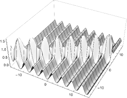
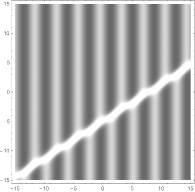
$\displaystyle t=2$:

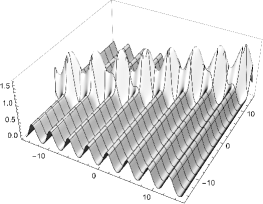
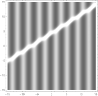
Figure 1: Line-soliton propagation with the elliptic background $\displaystyle u_{0}=-\wp(x)$ (the lemniscate case, $\displaystyle N=1$, $\displaystyle M=2$, $\displaystyle\tilde{a}_{1,1}=\tilde{a}_{1,2}=1$, $\displaystyle k_{1}=-3.2$, $\displaystyle k_{2}=-1.5$). In the graphs in the right column, the brighter the area, the larger the value of $\displaystyle u$.

$\displaystyle t=-2$:
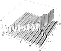
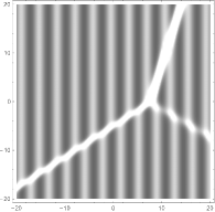
$\displaystyle t=2$:

Figure 2: Resonant interaction of line-solitons with the elliptic background $\displaystyle u_{0}=-\wp(x)$ (the lemniscate case, $\displaystyle N=1$, $\displaystyle M=3$, $\displaystyle\tilde{a}_{1,1}=\tilde{a}_{1,2}=\tilde{a}_{1,3}=1$, $\displaystyle k_{1}=-3.2$, $\displaystyle k_{2}=-1.5$, $\displaystyle k_{3}=-0.6$). In the graphs in the right column, the brighter the area, the larger the value of $\displaystyle u$.

$\displaystyle t=-1$:
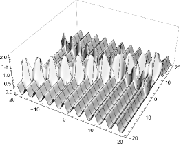
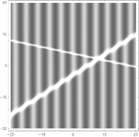
$\displaystyle t=1$:

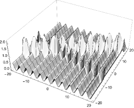
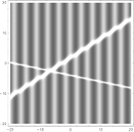
Figure 3: Interaction between two line-solitons with the elliptic background $\displaystyle u_{0}=-\wp(x)$ (the lemniscate case, $\displaystyle N=2$, $\displaystyle M=4$, $\displaystyle\tilde{A}$ is chosen as (6.15), $\displaystyle k_{1}=-3.2$, $\displaystyle k_{2}=-1.5$, $\displaystyle k_{3}=-0.6$, $\displaystyle k_{4}=-0.3$). In the graphs in the right column, the brighter the area, the larger the value of $\displaystyle u$.

$\displaystyle t=-2$:
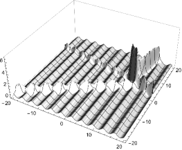
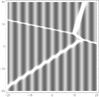
$\displaystyle t=0$:
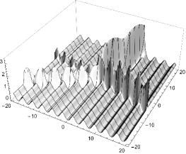
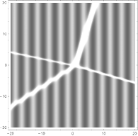
$\displaystyle t=2$:

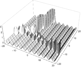
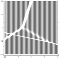
Figure 4: Example of complex interaction 1 (the lemniscate case, $\displaystyle N=2$, $\displaystyle M=4$, $\displaystyle\tilde{A}$ is chosen as $\displaystyle\tilde{A}_{1}$ of (6.16), $\displaystyle k_{1}=-3.2$, $\displaystyle k_{2}=-1.5$, $\displaystyle k_{3}=-0.6$, $\displaystyle k_{4}=-0.3$).

$\displaystyle t=-2$:
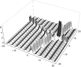
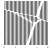
$\displaystyle t=0$:
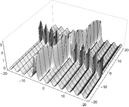
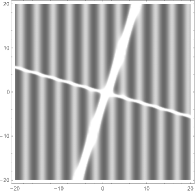
$\displaystyle t=2$:

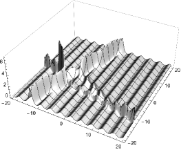
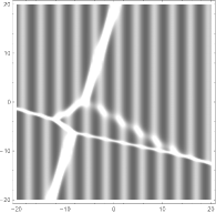
Figure 5: Example of complex interaction 2 (the lemniscate case, $\displaystyle N=2$, $\displaystyle M=4$, $\displaystyle\tilde{A}$ is chosen as $\displaystyle\tilde{A}_{2}$ of (6.16), $\displaystyle k_{1}=-3.2$, $\displaystyle k_{2}=-1.5$, $\displaystyle k_{3}=-0.6$, $\displaystyle k_{4}=-0.3$).

In the usual case without elliptic background, no sign change occurs in the usual plane wave factor $\displaystyle e^{\xi(x,\bm{t};k)}$ where $\displaystyle\xi(x,\bm{t};k)$ is defined by (2.20), and also in its higher order derivatives. This fact plays a major role in the classification of web-patterns [1, 14]. However, as can be seen in Figure 6, the sign change can occur for higher order derivatives of the real-valued Lamé-type plane wave factor (6.5), and it may induce zeros of the $\displaystyle\tau$-function (4.49), which may cause singularities of $\displaystyle u=\partial_{x}^{2}\left(\log\tau\right)$. A more detailed study is needed to classify web-like patterns of elliptic solitons.

$\displaystyle\tilde{\Phi}(x)$	$\displaystyle\tilde{\Phi}^{\prime}(x)$	$\displaystyle\tilde{\Phi}^{\prime\prime}(x)$

Figure 6: Graphs of the function $\displaystyle\tilde{\Phi}$ of (6.5) (the lemniscate case, $\displaystyle k=-1.2$)

Appendix

Examples of the differential operators $\displaystyle P_{n}$, $\displaystyle Q_{n-1}\in\mathcal{D}_{R}$ ($\displaystyle n=2,3,\ldots$):

$$\displaystyle P_{2} \displaystyle=\partial_{x}^{2}-2\wp(x),\quad Q_{1}=\wp(x)\partial_{x}-\frac{\wp^{\prime}(x)}{2},$$

$$\displaystyle P_{3} \displaystyle=\partial_{x}^{3}-3\wp(x)\partial_{x}-\frac{3\wp^{\prime}(x)}{2},\quad Q_{2}=\wp(x)\partial_{x}^{2}-\frac{\wp^{\prime}(x)}{2}\partial_{x}-\wp(x)^{2}-\frac{g_{2}}{4},$$

$$\displaystyle P_{4} \displaystyle=\partial_{x}^{4}-4\wp(x)\partial_{x}^{2}-4\wp^{\prime}(x)\partial_{x}+g_{2}-8\wp(x)^{2},$$

$$\displaystyle Q_{3} \displaystyle=\wp(x)\partial_{x}^{3}-\frac{\wp^{\prime}(x)}{2}\partial_{x}^{2}-2\wp(x)^{2}\partial_{x}-\wp(x)\wp^{\prime}(x),$$

$$\displaystyle P_{5} \displaystyle=\partial_{x}^{5}-5\wp(x)\partial_{x}^{3}-\frac{15\wp^{\prime}(x)}{2}\partial_{x}^{2}+3\left(g_{2}-10\wp(x)^{2}\right)\partial_{x}-15\wp(x)\wp^{\prime}(x),$$

$$\displaystyle Q_{4} \displaystyle=\wp(x)\partial_{x}^{4}-\frac{\wp^{\prime}(x)}{2}\partial_{x}^{3}-\left(\frac{g_{2}}{4}+3\wp(x)^{2}\right)\partial_{x}^{2}$$

$$\displaystyle\qquad-3\wp(x)\wp^{\prime}(x)\partial_{x}-g_{3}+\frac{g_{2}\wp(x)}{2}-6\wp(x)^{3},$$

$$\displaystyle P_{6} \displaystyle=\partial_{x}^{6}-6\wp(x)\partial_{x}^{4}-12\wp^{\prime}(x)\partial_{x}^{3}+\left(7g_{2}-72\wp(x)^{2}\right)\partial_{x}^{2}$$

$$\displaystyle\qquad-72\wp(x)\wp^{\prime}(x)\partial_{x}+2\left(-72\wp(x)^{3}+11g_{2}\wp(x)+8g_{3}\right),$$

$$\displaystyle Q_{5} \displaystyle=\wp(x)\partial_{x}^{5}-\frac{\wp^{\prime}(x)}{2}\partial_{x}^{4}-4\wp(x)^{2}\partial_{x}^{3}-6\wp(x)\wp^{\prime}(x)\partial_{x}^{2}$$

$$\displaystyle\qquad+\left(-2g_{3}+g_{2}\wp(x)-24\wp(x)^{3}\right)\partial_{x}-\frac{1}{2}\left(24\wp(x)^{2}+g_{2}\right)\wp^{\prime}(x).$$

Examples of the polynomials $\displaystyle R_{n}(x)$ ($\displaystyle n=0,1,2,\ldots$):

$$\displaystyle R_{0}(x) \displaystyle=x,\quad\frac{R_{1}(x)}{3!}=x^{2}-\frac{g_{2}}{12},\quad\frac{R_{2}(x)}{5!}=x^{3}-\frac{3g_{2}}{20}x-\frac{g_{3}}{10},$$

$$\displaystyle\frac{R_{3}(x)}{7!} \displaystyle=x^{4}-\frac{g_{2}}{5}x^{2}-\frac{g_{3}}{7}x+\frac{g_{2}^{2}}{560},$$

$$\displaystyle\frac{R_{4}(x)}{9!} \displaystyle=x^{5}-\frac{g_{2}}{4}x^{3}-\frac{5g_{3}}{28}x^{2}+\frac{g_{2}^{2}}{120}x+\frac{11g_{2}g_{3}}{1680},$$

$$\displaystyle\frac{R_{5}(x)}{11!} \displaystyle=x^{6}-\frac{3g_{2}}{10}x^{4}-\frac{3g_{3}}{14}x^{3}+\frac{7g_{2}^{2}}{400}x^{2}+\frac{57g_{2}g_{3}}{3080}x-\frac{g_{2}^{3}}{26400}+\frac{g_{3}^{2}}{308}.$$

Examples of the differential operators $\displaystyle\tilde{P}_{n}\in\mathcal{D}_{R}$ ($\displaystyle n=2,3,\ldots$):

$$\displaystyle\tilde{P}_{2} \displaystyle=P_{2}=\partial_{x}^{2}-2\wp(x),\quad\tilde{P}_{3}=P_{3}=\partial_{x}^{3}-3\wp(x)\partial_{x}-\frac{3\wp^{\prime}(x)}{2},$$

$$\displaystyle\tilde{P}_{4} \displaystyle=P_{4}-\frac{g_{2}}{12}=\partial_{x}^{4}-4\wp(x)\partial_{x}^{2}-4\wp^{\prime}(x)\partial_{x}+\frac{11g_{2}}{12}-8\wp(x)^{2},$$

$$\displaystyle\tilde{P}_{5} \displaystyle=P_{5}=\partial_{x}^{5}-5\wp(x)\partial_{x}^{3}-\frac{15\wp^{\prime}(x)}{2}\partial_{x}^{2}+3\left(g_{2}-10\wp(x)^{2}\right)\partial_{x}-15\wp(x)\wp^{\prime}(x),$$

$$\displaystyle\tilde{P}_{6} \displaystyle=P_{6}-\frac{3g_{2}}{20}P_{2}-\frac{g_{3}}{10}$$

$$\displaystyle=\partial_{6}-6\wp(x)\partial_{x}^{4}-12\wp^{\prime}(x)\partial_{x}^{3}+\left\{\frac{137g_{2}}{20}-72\wp(x)^{2}\right\}\partial_{x}^{2}$$

$$\displaystyle\qquad\qquad-144\wp(x)^{3}-72\wp(x)\wp^{\prime}(x)\partial_{x}+\frac{1}{10}\left(223g_{2}\wp(x)+159g_{3}\right).$$

References

[1]
S. Chakravarty and Y. Kodama,
Soliton solutions of the KP equation and application to shallow water waves,
Stud. Appl. Math.123 (2009), 83–151.
[2]
L.-L. Chau, J.C. Shaw and H.C. Yen,
Solving the KP hierarchy by gauge transformations,
Comm. Math. Phys.149 (1992), 263–278.
[3]
J. Chen, D.E. Pelinovsky and R.E. White,
Rogue waves on the double-periodic background in the
focusing nonlinear Schrödinger equation,
Phys. Rev. E100 (2019), 052219.
[5]
E. Date, M. Kashiwara, M. Jimbo and T. Miwa,
Transformation groups for soliton equations,
in Proceedings of RIMS symposium on non-linear integrable system
— classical theory and quantum theory, M. Jimbo and T. Miwa (eds.),
World Science Publishing Co., Singapore, 1983, pp. 39–119.
[7]
B.-F. Feng, L. Ling and D.A. Takahashi,
Multi-breather and high-order rogue waves for the nonlinear Schrödinger equation
on the elliptic function background,
Stud. Appl. Math.144 (2020), 46–101.
[8]
G.F. Helminck and J.W. van de Leur,
An analytic description of the vector constrained KP hierarchy,
Comm. Math Phys.193 (1998), 627–641.
[9]
G.F. Helminck and J.W. van de Leur,
Darboux transformations for the KP hierarchy in the Segal-Wilson setting,
Canad. J. Math.53 (2001) 278–309.
[10]
G.F. Helminck and J.W. van de Leur,
Geometric Bäcklund-Darboux transformations for the KP hierarchy,
Publ. RIMS, Kyoto Univ.37 (2001), 479–519.
[11]
T. Ichikawa,
Tau functions and KP solutions on families of algebraic curves,
arXiv preprint (arXiv:2208.07013).
[12]
S. Isojima, R. Willox and J. Satsuma,
Spider-web solutions of the coupled KP equation,
J. Phys. A: Math. Gen.36 (2003), 9533–9552.
[13]
M. Jimbo and T. Miwa,
Solitons and infinite dimensional Lie algebras,
Publ. RIMS, Kyoto Univ.19 (1983), 943–1001.
[14]
Y. Kodama,
KP Solitons and the Grassmannians: Combinatorics and Geometry of Two-Dimensional Wave Patterns,
Springer Briefs in Mathematical Physics 22, Springer (2017).
[15]
I.M. Krichever,
Elliptic solutions of the Kadomtsev-Petviashvili equations,
and integrable systems of particles,
Funktsional. Anal. i Prilozhen14 (1980), 45–54
(English transl.: Funct. Anal. Appl.14 (1980), 282–290).
[16]
E.A. Kuznetsov and A.V. Mikhailov,
Stability of stationary waves in nonlinear weakly dispersive media,
Zh. Eksp. Teor. Fiz.67 (1974), 1717–1727
(English transl.: Sov. Phys. JETP40 (1975), 855–859).
[17]
X. Li and D.-j. Zhang,
Elliptic soliton solutions: functions, vertex operators and bilinear identities,
J. Nonlin. Sci.32 (2022), Article number 70.
[18]
X. Li and D.-j. Zhang,
The Lamé functions and elliptic soliton solutions: Bilinear approach,
arXiv preprint (arXiv:2307.02312).
[19]
D. Levi and O. Ragnisco,
Dressing method and Bäcklund and Darboux transformations,
in Bäcklund and Darboux Transformations:
The Geometry of Sollitons,
CRM Proceedings and Lecture Notes 29, (2001), pp. 29–51.
[20]
K. Maruno and G. Biondini,
Resonance and web structure in discrete soliton systems:
the two-dimensional Toda lattice and its fully discrete and ultra-discrete versions,
J. Phys. A: Math. Gen.37 (2004), 11819-11840.
[21]
V.B. Matveev and M.A. Salle,
Darboux transformations and solitons,
Springer Series in Nonlinear Dynamics 17,
Berlin, Springer, 1991.
[22]
S. Matsutani,
Hyperelliptic solutions of KdV and KP equations:
re-evaluation of Baker’s study on hyperelliptic sigma functions,
J. Phys. A: Math. Gen.34 (2001), 4721–4732.
[23]
T. Miwa, M. Jimbo and E. Date,
Solitons: Differential Equations, Symmetries and Infinite Dimensional Algebras,
translated by M. Reid,
Cambridge Tracts in Mathematics 135,
Cambridge University Press (1999).
[24]
A. Nakayashiki,
Sigma function as a tau function,
Int. Math. Res. Not.2010 (2010), 373–394.
[25]
A. Nakayashiki,
One step degeneration of trigonal curves and mixing of solitons and
quasi-periodic solutions of the KP equation,
In Geometric Methods in Physics XXXVIII,
P. Kielanowski, A. Odzijewicz, E. Previato (eds.),
Trends in Math., Birkhäuser, Cham. (2020), pp. 163–186.
[26]
A. Nakayashiki,
Vertex operators of the KP hierarchy and singular algebraic curves,
arXiv preprint (arXiv:2309.08850).
[27]
F.W. Nijhoff and J. Atkinson,
Elliptic -soliton solutions of ABS lattice equations,
Int. Math. Res. Not.2010 (2010), 3837–3895.
[28]
W. Oevel,
Darboux theorems and Wronskian formulas for
integrable systems: I. Constrained KP flows,
Physica A195 (1993), 533–576.
[29]
W. Oevel and C. Rogers,
Gauge transformations and reciprocal links in dimensions,
Rev. Math. Phys.5 (1993), 299–330.
[30]
W. Oevel and W. Schief,
Darboux theorems and the KP hierarhcy,
in Applications of Analytic and Geometric Methods to Nonlinear
Differential Equations,
P.A. Clarkson (ed.), Kluwer Publ. (1993), pp. 193–206.
[31]
Y. Ohta, J. Satsuma, D. Takahashi and T. Tokihiro,
An elementary introduction to Sato theory,
Prog. Theor. Phys. Suppl.94 (1988), 210–241
(Addenda: Prog. Theor. Phys.80 (1988), 742).
[32]
G. Pastras,
The Weierstrass Elliptic Function and Applications in Classical and Quantum Mechanics
— A Primer for Advanced Undergraduates,
Springer Briefs in Physics, Springer (2020).
[33]
M. Sato,
Soliton equations as dynamical systems on an infinite dimensional Grassmann manifolds,
RIMS Kokyuroku, Kyoto Univ.439 (1981), 30–46.
[34]
M. Sato and Y. Sato,
Soliton equations as dynamical systems on an infinite dimensional Grassmann manifold,
in Nonlinear Partial Differential Equations in Applied Sciences, U.S.-Japan seminar, Tokyo 1982,
P.D. Lax, H. Fujita, and G. Strang (eds.),
North-Holland, Amsterdam and Kinokuniya, Tokyo, 1982, pp. 259–271.
[35]
M. Sato,
The KP hierarchy and infinite-dimensional Grassmann manifolds,
in Theta Functions, Bowdoin 1987 (Brunswick, ME, 1987),
Proc. Sympos. Pure Math.49, Part 1 (1989), pp. 51–66.
[36]
A.B. Shabat,
On the Korteweg-de Vries equation,
Dokl. Akad. Nauk SSSR211, No. 6 (1973), 1310–1313
(in Russian).
[37]
A.O. Smirnov,
Elliptic solutions of the KdV equation,
Mat. Zametki [Math. Notes] 45, No. 6 (1989), 66–73.
[38]
T.H. Southard,
§18. Weierstrass elliptic and related functions,
in Handbook of Mathematical Functions with Formulas, Graphs, and Mathematical Tables,
M. Abramowitz and I.A. Stegun (eds.),
9th printing, Dover, New York (1972).
[39]
D.A. Takahashi,
Integrable model for density-modulated quantum condensates:
solitons passing through a soliton lattice,
Phys. Rev. E93 (2016), 062224.
[40]
A. Treibich and J.-L. Verdier,
Solitons elliptiques, Progr. Math. (The Grothendieck Festschrift,
vol. 3). v.88.
Birkhäuser, Boston (1990), pp. 437–480.
[41]
E.T. Whittaker and G.N. Watson,
A course of modern analysis,
Fifth edition, Cambridge University Press (2021).
[42]
S. Yoo-Kong and F. Nijhoff,
Elliptic -soliton solutions of the lattice Kadomtsev-Petviashvili equation,
J. Math. Phys.54 (2013), 043511.