Enhancing modified treatment policy effect estimation with weighted energy distance

Abstract

The effects of continuous treatments are often characterized through the average dose response function, which is challenging to estimate from observational data due to confounding and positivity violations. Modified treatment policies (MTPs) are an alternative approach that aim to assess the effect of a modification to observed treatment values and work under relaxed assumptions. Estimators for MTPs generally focus on estimating the conditional density of treatment given covariates and using it to construct weights. However, weighting using conditional density models has well-documented challenges. Further, MTPs with larger treatment modifications have stronger confounding and no tools exist to help choose an appropriate modification magnitude. This paper investigates the role of weights for MTPs showing that to control confounding, weights should balance the weighted data to an unobserved hypothetical target population, that can be characterized with observed data. Leveraging this insight, we present a versatile set of tools to enhance estimation for MTPs. We introduce a distance that measures imbalance of covariate distributions under the MTP and use it to develop new weighting methods and tools to aid in the estimation of MTPs. We illustrate our methods through an example studying the effect of mechanical power of ventilation on in-hospital mortality.
Keywords— Continuous Treatments, Covariate Balance, Balancing weights, Causal Inference, Observational Studies

1 Introduction

Understanding the causal effects of changes in doses or otherwise continuous values of a treatment is important in many scientific disciplines. A typical approach to quantifying the causal effect of varying a continuous treatment is to estimate the causal average dose response function (ADRF), which is the expected potential outcome as a function of all possible or likely treatment values. In our motivating example, the treatment is the mechanical power of a ventilator applied to patients in intensive care who have acute respiratory distress syndrome. In this setting, the ARDF is the expected in-hospital mortality as a function of the power of ventilation. While the ADRF provides an intuitive way to evaluate the causal effect of a continuous treatment, its estimation requires one to assume that every individual could hypothetically receive all possible values of the treatment, which is often unlikely in practice as some values may be clinically unlikely or impossible for subsets of the population. Moreover, confounding is exacerbated in causal ADRF estimation because the characteristics of subjects with a higher treatment value may differ substantively from those with a lower value. Additionally, the performance of causal ADRF estimators is often poor (i.e. cannot attain root-$n$ consistency nonparametrically), even with flexible, doubly robust methods (Kennedy et al., 2017).

Alternative definitions of causal effects in this setting have been introduced in part to help alleviate some of these problems while still providing clinically useful results. D\́boldsymbol{i}az and van der Laan (2013) proposed the concept of stochastic interventions which estimates the effect of assigning each subject’s intervention based on a random draw from a given distribution depending on their own characteristics. Haneuse and Rotnitzky (2013) further proposed modified treatment policies (MTPs) which generalize the idea of stochastic interventions. Each subject’s counterfactual treatment under a given MTP is defined as a function of their baseline characteristics and their observed values of the treatment without the MTP (the “natural” value of the treatment); the MTP thus imagines a slight manipulation of each individual’s treatment value from their actual values. The estimand is then defined as the expected potential outcome under the specified manipulation. For example, in our motivating application, one could estimate the effect of slightly reducing or increasing the mechanical power of ventilation, compared with standard of care, on in-hospital mortality among patients in the intensive care unit (ICU) who have acute respiratory distress (Neto et al., 2018).

Although an MTP cannot be implemented precisely in practice, it can help policymakers evaluate hypotheses about the treatment and generate practical interventions that can be later tested via experiments. Another advantage of MTPs is that, by imagining counterfactual worlds where the treatment is modified slightly from reality, the corresponding counterfactual world is not substantially different from reality, making positivity hold by construction. D\́boldsymbol{i}az et al. (2021) generalized MTPs to longitudinal data and proposed efficient estimators for the causal effect. D\́boldsymbol{i}az and Hejazi (2020) used stochastic interventions for causal mediation analysis. MTPs are thus an attractive tool for causal inference as they can be quite general and can be used in a wide variety of settings.

Confounding is a major hurdle in causal inference from observational studies, both for standard estimands and for MTPs. Weighting approaches to confounding control re-weight each subject to balance the distribution of the covariates and do not require the use of outcome information. Traditionally, weights are generated through inverse-probability weighting (IPW) which models the treatment assignment mechanism given covariates and inverts it. However, the performance of IPW relies critically on the choice of the propensity score model and model misspecification can result in severe bias (Kang and Schafer, 2007). Alternative weighting methods have been proposed to mitigate this issue in the setting of estimating standard causal effects of discrete-valued treatments by using weights that encourage (Imai and Ratkovic, 2014) or enforce (Hainmueller, 2012) balance of pre-specified moments of covariates. Particularly relevant to our article is the work by Huling and Mak (2020) who consider weights that minimize the energy distance between the weighted empirical distribution of the intervention groups and the joint population, aiming to balance the full joint distributions of covariates. This nonparametric distributional balancing approach has been shown to work empirically well with no need for careful modeling decisions.

Several challenging issues remain unresolved for weighting methods for MTPs. Existing weighting methods for MTPs have focused on the estimation of the conditional density of treatment given the covariates, also known as the generalized propensity score (GPS). D\́boldsymbol{i}az and van der Laan (2013) and Haneuse and Rotnitzky (2013) both proposed weighting estimators based on estimation of the GPS. These methods show great promise, but their success hinges on accurately specifying the conditional density model. Yet, estimating a conditional density is highly challenging especially with an increasing number of covariates (Huling et al., 2023). Even slight misspecification of the estimated density function from the truth function can impact the performance of the IPW-style estimators of the ADRF (Naimi et al., 2014); these issues persist in the estimation of MTPs. Moreover, the impact of weights on finite sample performance is not yet fully understood and no diagnostic tools are available to assess the performance of a given set of weights or to understand whether a given set of weights is likely to yield an unconfounded comparison for a given dataset. As MTPs involve investigating the effect of a shift of treatment values from their observed values, larger shifts are likely to yield analyses with more confounding and with more potential for positivity violations. Yet no tools exist that can assess what range of shifts in a class of MTPs are “safe” (i.e. have confounding that can be fully adjusted using a given weighting method) for a given application. Clear guidance is thus needed for practitioners to determine an appropriate magnitude of the MTP shift.

In this work, we introduce distance-based tools that provide solutions to the aforementioned issues. By examining the role of the weights in finite sample error of a generic weighting estimator, we show that confounding bias depends on the distributional distance between the observed population (the real world) and the population induced by a given MTP (the counterfactual world). Towards this aim, we first extend the identification result of the modified treatment policy from Haneuse and Rotnitzky (2013) to clarify the form of the target counterfactual population for an MTP and provide a clear mathematical expression of it. Even though the target population is purely hypothetical, we show its distribution can be estimated using the observed data, a fact used extensively in our methods. We then present a novel error decomposition to show that the estimation error of a weighted estimate of the causal effect of MTP is directly related to the imbalance of the weighted empirical distribution (referring to the empirical distribution of the weighted observed sample) and the targeted empirical distribution induced by an MTP. We provide a measure of this distance with a modification of the energy distance (Székely and Rizzo, 2013), a computationally simple measure of the distance between two multivariate distributions. It has been used to measure distributional imbalance in the context of categorical treatments (Huling and Mak, 2020) and to quantify dependence between continuous treatments and confounders (Huling et al., 2023). We propose a set of energy distance-based tools to enhance the estimation of MTP effects. Specifically, our methods provide 1) an assessment of a feasible range of shifts for a class of MTPs for arbitrary weighting methods for a given dataset and 2) a comparison of different weighting methods for MTPs. Finally, we introduce energy balancing weights which have optimal reduction of distributional imbalance to the target population, providing a new robust weighting approach for MTP estimation.

The remainder of this article is as follows. In Section 2, we describe the MTP framework and propose a novel error decomposition to reveal the relationship between the estimation bias and distributional imbalance. Section 3 introduces our modification of the energy distance. In Section 4, we propose energy-distance-based methods for evaluating the feasibility of an MTP and for evaluating different weighting methods. In Section 5, we propose new weights that directly balance data to the target distribution. In Section 6, we introduce an augmented estimator based on the energy balancing weights and show its asymptotic normality in estimating the MTP effect. We also propose a multiplier bootstrap method that is more computationally efficient in estimating the uncertainty of the augmented estimator and provide statistical guarantees for its use. We illustrate the robust performance of our proposed estimators through extensive numerical experiments in Section 7. In Section 8, we illustrate the use of our proposed set of methods through a real example of the mechanical power of ventilation.

2 Setup

2.1 Causal framework for modified treatment policies (MTPs)

Consider data $\{{\boldsymbol{X}}_{i},A_{i},Y_{i}\}_{i=1}^{n}$ collected from an observational study, where ${\boldsymbol{X}}_{i}\in\mathcal{X}\subseteq\mathbb{R}^{p}$ denotes a p-dimensional vector of pre-treatment covariates for subject $i$, $A_{i}\in\mathcal{A}\subseteq\mathbb{R}$ denotes the received value of the treatment, and $Y_{i}\in\mathbb{R}$ denotes the outcome. Here we assume $A_{i}$ is a continuous treatment variable (e.g., the taken dose of a treatment for individual $i$). We adopt the potential outcome framework in which we assume that for each subject $i$, there exists a potential outcome $Y^{a}_{i}$ defined as the outcome that subject $i$ would have if subject $i$ is intervened on to take the treatment at value $A=a$. An MTP analysis starts with an analyst-specified treatment policy $q({\bf x},a)$ that inputs patient characteristics and observed treatment values and outputs a modified value of the treatment. The goal of an MTP analysis is to estimate the mean potential outcome $\mu^{q}\equiv\mathbb{E}[Y^{q({\boldsymbol{X}},A)}]$ under this policy; this can then be contrasted with the average observed outcome $\mathbb{E}[Y^{A}]=\mathbb{E}[Y]$ to understand whether the policy improves or harms outcomes on average. To ensure $Y^{a}_{i}$ is well-defined (i.e, $Y^{a}_{i}$ is unique for a given treatment level $a$ and subject $i$), we assume the following consistency condition:

• (A0 Consistency): For any subject $i$ in the population, if $A_{i}=a$ then $Y_{i}=Y^{a}_{i}$.

It is not realistic for some patients to have extreme values of treatment, e.g. extremely low mechanical power of ventilation for patients who have serious respiratory symptoms (see section 8 for the case study). As such, as in the work of Haneuse and Rotnitzky (2013), we define the enforceable set $\mathcal{A}_{i}$ for subject $i$ to be the set of treatment values that the potential outcomes are meaningful for the subject. We further assume that the enforceable set for subject $i$ is fully determined by the treatment value received $A_{i}$ and the covariates ${\boldsymbol{X}}_{i}$, i.e, $\mathcal{A}_{i}=\mathcal{A}({\boldsymbol{X}}_{i},A_{i})$. Using the enforceable set, we can work with a positivity assumption that is reasonable even in the presence of strong confounding. For example, if there is a positive density of observing subject $i$ with covariate ${\boldsymbol{x}}_{i}$ and treatment $a_{i}$, then it is reasonable to assume that we have a positive density to observe a subject with the same covariate ${\boldsymbol{x}}_{i}$ and treatment value $a\in\mathcal{A}({\boldsymbol{x}}_{i},a_{i})$. In contrast, calculating the causal effect of an arbitrary treatment value $a$ may not be meaningful since this treatment value may not be feasible or applicable to the entire population. Therefore, we focus on estimating the causal effects of an MTP that modifies or shifts the observed treatment values to be within the enforceable set.

Since the enforceable set is determined by ${\boldsymbol{X}}$ and $A$, the MTP can be designed to be realistic for the entire population, i.e., the treatment policy $q({\boldsymbol{x}},a)\in\mathcal{A}({\boldsymbol{x}},a)$ for any $({\boldsymbol{x}},a)\in(\mathcal{X},\mathcal{A})$, where $(\mathcal{X},\mathcal{A})$ be the joint support of the random variables ${\boldsymbol{X}}$ and $A$. It is important to note that MTPs are distinct from dynamic treatment regimes, where the current treatment values are determined by the past treatment values. MTPs, on the other hand, define the modified treatment value based on the natural (observed) treatment value without intervention. This means that the modified treatment value and the natural treatment value are supposed to happen at the same time, and since we do not know the actual treatment value without intervention, the MTP cannot be implemented exactly in practice. However, MTPs are still pertinent to clinical practice, as they can provide insight into how modifications to clinical practice could have changed patient outcomes. By considering the effects of a collection of MTPs, researchers can gain insights into the underlying mechanisms that lead to different outcomes and identify potential strategies for improving patient outcomes. For example, to evaluate a care policy that encourages a slight reduction in intensity of mechanical ventilation, we could estimate the causal effect of the MTP $q({\boldsymbol{x}},a)=a-2$ which reduced mechanical power for all subjects by 2 Joules/min compared with current standards. The MTP could be further refined to modify the amount of reduction differently for people with different characteristics or prior ventilation patterns.

For any $({\boldsymbol{x}},a)\in(\mathcal{X},\mathcal{A})$, we can define $\mathbb{E}(Y^{q({\boldsymbol{x}},a)}|{\boldsymbol{X}}={\boldsymbol{x}},A=a)$ to be the expected potential outcome averaging over all subjects who have ${\boldsymbol{X}}={\boldsymbol{x}},A=a$. The mean potential outcome of the MTP $q({\boldsymbol{x}},a)$ is then the mean of the conditional average potential outcome $\mathbb{E}(Y^{q({\boldsymbol{x}},a)}|{\boldsymbol{X}}={\boldsymbol{x}},A=a)$ over the entire population, i.e.,

$$\mu^{q}:=\int_{(\mathcal{X},\mathcal{A})}\mathbb{E}[Y^{q({\boldsymbol{x}},a)}|{\boldsymbol{X}}={\boldsymbol{x}},A=a]dF_{{\boldsymbol{X}},A}({\boldsymbol{x}},a)$$ (1)

where $F_{{\boldsymbol{X}},A}({\boldsymbol{x}},a)$ is the distribution function of $({\boldsymbol{X}},A)$. In order to make the integral well-defined, we follow Haneuse and Rotnitzky (2013) to assume the continuity of $\mathbb{E}[Y^{q({\boldsymbol{x}},a)}|{\boldsymbol{X}}={\boldsymbol{x}},A=a]$ over $({\boldsymbol{x}},a)\in(\mathcal{X},\mathcal{A})$ and continuity of $A|{\boldsymbol{X}}={\boldsymbol{x}}$ over ${\boldsymbol{x}}\in\mathcal{X}$. In order to estimate the causal effect from observational data, $\mu^{q}$ needs to be causally-identifiable. In other words, we need to express $\mu^{q}$ as a function of the distribution of $(Y,{\boldsymbol{X}},A)$. From Haneuse and Rotnitzky (2013), $\mu^{q}$ can be identified with the following assumptions:

• (A1 Positivity): If $({\boldsymbol{x}},a)\in(\mathcal{X},\mathcal{A})$ then $({\boldsymbol{x}},q({\boldsymbol{x}},a))\in(\mathcal{X},\mathcal{A})$.

• (A2 Conditional exchangeability of related populations) For each $({\boldsymbol{x}},a)\in(\mathcal{X},\mathcal{A})$, let $a^{\prime}=q({\boldsymbol{x}},a)$, then $Y^{a^{\prime}}|{\boldsymbol{X}}={\boldsymbol{x}},A=a$ and $Y^{a^{\prime}}|{\boldsymbol{X}}={\boldsymbol{x}},A=a^{\prime}$ have the same distribution.

The positivity assumption states that for each subject in the population, it is always possible to find some other subjects who have the same covariates and receive the modified treatment. The second assumption state that the potential outcome of the modified treatment will not be affected by the original treatment allocation. In other words, subjects with ${\boldsymbol{X}}={\boldsymbol{x}}$ who received treatment $a$ could have received treatment $q({\boldsymbol{x}},a)$. The difference between A2 and the usual no-unmeasured confounders assumption is that the latter is much stronger, as it requires the subjects with ${\boldsymbol{X}}={\boldsymbol{x}}$ who received treatment $a$ could have received any possible dose $a^{\prime}\in\mathcal{A}_{{\boldsymbol{x}}}$ where $\mathcal{A}_{{\boldsymbol{x}}}:=\{a:({\boldsymbol{x}},a)\in(\mathcal{X},\mathcal{A})\}$ be the support of $A$ given ${\boldsymbol{X}}={\boldsymbol{x}}$.

In order to have a closed-form derivation of our proposed estimator, we further restrict the MTP to have a piecewise differentiable inverse function.

• (A3 Piece-wise smooth invertibility): For each ${\boldsymbol{x}}\in\mathcal{X}$, there exists a partition $\{I_{j,{\boldsymbol{x}}}\}_{j=1}^{J({\boldsymbol{x}})}$ of $\mathcal{A}_{{\boldsymbol{x}}}$ where $q({\boldsymbol{x}},\cdot)$ is smooth and invertible within the partition. Specifically, let $q_{j}({\boldsymbol{x}},\cdot)$ denote the function $q({\boldsymbol{x}},\cdot)$ on the $I_{j,{\boldsymbol{x}}}$ part. Then $q_{j}({\boldsymbol{x}},\cdot)$ has differentiable inverse function $h_{j}({\boldsymbol{x}},\cdot)$ on the interior of $I_{j,{\boldsymbol{x}}}$, such that $h_{j}({\boldsymbol{x}},q_{j}({\boldsymbol{x}},a))=a$

Under Assumption A3, for a given ${\boldsymbol{x}}\in\mathcal{X}$, the MTP $q({\boldsymbol{x}},a)$ can be expressed as the sum of the functions $\{q_{j}({\boldsymbol{x}},a)\}_{j=1}^{J({\boldsymbol{x}})}$ on each interval $\{I_{j,{\boldsymbol{x}}}\}_{j=1}^{J({\boldsymbol{x}})}$, $q({\boldsymbol{x}},a)=\sum_{j=1}^{J({\boldsymbol{x}})}I_{j,{\boldsymbol{x}}}(a)q_{j}({\boldsymbol{x}},a)$ where $I_{j,{\boldsymbol{x}}}(a)$ be the indicator function s.t. $I_{j,{\boldsymbol{x}}}(a)=1$ if $a\in I_{j,{\boldsymbol{x}}}$ and $I_{j,{\boldsymbol{x}}}(a)=0$ otherwise. Assumption A3 is important, as it allows us to cleanly express the expected potential outcome under the MTP as a function of the observed data distribution. With the assumption of the piece-wise smooth invertibility, we have the following identification result from Haneuse and Rotnitzky (2013),

$$\mu^{q}=\int_{\mathcal{X}}\sum_{j=1}^{J({\boldsymbol{x}})}\int_{h_{j}({\boldsymbol{x}},a)\in I_{j,{\boldsymbol{x}}}}\mathbb{E}(Y|{\boldsymbol{X}}={\boldsymbol{x}},A=a)dF_{{\boldsymbol{X}},A}({\boldsymbol{x}},h_{j}({\boldsymbol{x}},a)).$$ (2)

The proof which follows similar arguments as Haneuse and Rotnitzky (2013) is presented in the Supplementary Material.

2.2 Novel error decomposition for weighted MTP estimators

In this section, we present a novel error decomposition that allows a clear inspection of the role of sample weights in finite sample errors when estimating $\mu^{q}$ using weighting methods. This decomposition provides insights that enable us to provide a measure of confounding bias as a function of the sample weights. This measure then allows us to provide tools that compare weights and further tools to assess when a given MTP is so far from the observed treatments that measured confounding is excessive and/or too difficult to control with weights.

Denoting $\mu({\boldsymbol{x}},a)\equiv\mathbb{E}(Y|{\boldsymbol{X}}={\boldsymbol{x}},A=a)$, we have $Y_{i}=\mu({\boldsymbol{X}}_{i},A_{i})+{\epsilon}_{i}$ where $\epsilon_{i}\equiv Y_{i}-\mu({\boldsymbol{X}}_{i},A_{i})$ is independent of ${\boldsymbol{X}}_{i}$ and $A_{i}$ with mean zero. We can express the estimand (2) as

$$\mu^{q}=\int_{(\mathcal{X},\mathcal{A})}\mu({\boldsymbol{x}},a)dF_{{\boldsymbol{X}},A}^{q}({\boldsymbol{x}},a),\text{ where}$$ (3)

$$F_{{\boldsymbol{X}},{\boldsymbol{A}}}^{q}({\boldsymbol{x}},a)=\sum_{j=1}^{J({\boldsymbol{x}})}I_{j,{\boldsymbol{x}}}(h_{j}({\boldsymbol{x}},a))F_{{\boldsymbol{X}},A}({\boldsymbol{x}},h_{j}({\boldsymbol{x}},a))$$ (4)

and $F_{{\boldsymbol{X}},A}({\boldsymbol{x}},a)$ is the CDF of $({\boldsymbol{X}},A)$. In the Supplementary Materials, we prove that $F_{{\boldsymbol{X}},{\boldsymbol{A}}}^{q}({\boldsymbol{x}},a)$ is the CDF of $({\boldsymbol{X}},q({\boldsymbol{X}},A))$, as long as $q({\bf x},a)$ has the property that $\lim_{({\boldsymbol{x}},a)\to\boldsymbol{-\infty}}q({\boldsymbol{x}},a)=\boldsymbol{-\infty}$ and $\lim_{({\boldsymbol{x}},a)\to\boldsymbol{\infty}}q({\boldsymbol{x}},a)=\boldsymbol{\infty}$.

In this paper, we focus on weighted estimators of $\mu^{q}$ which do not require one to use outcome information, allowing the analyst to conduct objective causal inference. A weighting estimator with arbitrary sample weights ${\boldsymbol{w}}=(w_{1},...,w_{n})$ can be expressed as: $\hat{\mu}^{q}_{{\boldsymbol{w}}}=\frac{1}{n}\sum_{i=1}^{n}w_{i}Y_{i}=\frac{1}{n}\sum_{i=1}^{n}w_{i}\mu({\boldsymbol{X}}_{i},A_{i})+\frac{1}{n}\sum_{i=1}^{n}w_{i}\epsilon_{i}$ where $\sum_{i=1}^{n}w_{i}=n$. This weighted estimator can be expressed as

$$\hat{\mu}^{q}_{{\boldsymbol{w}}}=\int_{(\mathcal{X},\mathcal{A})}\mu({\boldsymbol{x}},a)dF_{n,{\boldsymbol{w}},{\boldsymbol{X}},A}+\frac{1}{n}\sum_{i=1}^{n}w_{i}\epsilon_{i},$$

where $F_{n,{\boldsymbol{w}},{\boldsymbol{X}},{\boldsymbol{A}}}=\frac{1}{n}\sum_{i=1}^{n}w_{i}I({\boldsymbol{X}}_{i}\leq{\boldsymbol{x}},A_{i}\leq a)$ is the weighted empirical CDF of the sample.

We can express the error of the weighted estimator $\hat{\mu}^{q}_{{\boldsymbol{w}}}$ as:

$$\hat{\mu}^{q}_{{\boldsymbol{w}}}-\mu^{q}={} \underbrace{\int_{(\mathcal{X},\mathcal{A})}\mu({\boldsymbol{x}},a)d(F_{n,{\boldsymbol{w}},{\boldsymbol{X}},A}-F_{n,{\boldsymbol{X}},A}^{q})({\boldsymbol{x}},a)}_{\text{error due to confounding bias}}$$ (5)

$$+\underbrace{\int_{(\mathcal{X},\mathcal{A})}\mu({\boldsymbol{x}},a)d(F_{n,{\boldsymbol{X}},A}^{q}-F_{{\boldsymbol{X}},A}^{q})}_{\text{sampling error}}+\frac{1}{n}\sum_{i=1}^{n}w_{i}\epsilon_{i},$$ (6)

where $F_{n,{\boldsymbol{X}},A}^{q}({\boldsymbol{x}},a)=\frac{1}{n}\sum_{i=1}^{n}\sum_{j=1}^{J({\boldsymbol{X}}_{i})}I_{j,{\boldsymbol{X}}_{i}}(A_{i})I({\boldsymbol{X}}_{i}\leq{\boldsymbol{x}},q_{j}({\boldsymbol{X}}_{i},A_{i})\leq a)$ is the empirical estimator of the shifted distribution $F_{{\boldsymbol{X}},A}^{q}$. The error decomposition emphasizes the importance of sample weights in mitigating confounding bias. The second term depends on how well the CDF can be estimated using the empirical CDF. The third term is affected by the variance of the weights, however, it always has mean $0$. Thus, confounding bias can be mitigated by minimizing the first term $\int_{(\mathcal{X},\mathcal{A})}\mu({\boldsymbol{x}},a)d(F_{n,{\boldsymbol{w}},{\boldsymbol{X}},A}-F_{n,{\boldsymbol{X}},A}^{q})({\boldsymbol{x}},a)$ which measures the distance between the two distribution functions.

Note that $F_{n,{\boldsymbol{X}},A}^{q}({\boldsymbol{x}},a)$ is the empirical CDF of the random variable $({\boldsymbol{X}},q({\boldsymbol{X}},A))$ and $F_{n,{\boldsymbol{w}},{\boldsymbol{X}},A}({\boldsymbol{x}},a)=\frac{1}{n}\sum_{i=1}^{n}w_{i}I({\boldsymbol{X}}_{i}\leq{\boldsymbol{x}},A_{i}\leq a)$ is the weighted empirical CDF of random variable $({\boldsymbol{X}},A)$. Thus, the term $\int_{(\mathcal{X},\mathcal{A})}\mu({\boldsymbol{x}},a)d(F_{n,{\boldsymbol{w}},{\boldsymbol{X}},A}-F_{n,{\boldsymbol{X}},A}^{q})({\boldsymbol{x}},a)$ depends on both the weights ${\boldsymbol{w}}$ and the pre-specified modified treatment policy $q({\boldsymbol{x}},a)$. Larger shifts on the MTP will lead to the larger difference between the distribution of $({\boldsymbol{X}},q({\boldsymbol{X}},A))$ and $({\boldsymbol{X}},A)$ which makes the confounding bias term larger, generally speaking.

3 Weighted Energy Distance for MTPs

After identifying the key component of confounding bias in estimating the causal effect of MTP, a natural question arises: can we measure or bound its magnitude for a given set of weights? Doing so would enable objective evaluation of a set of weights in the specific context of a given MTP for a given dataset. Since the confounding bias component $\int_{(\mathcal{X},\mathcal{A})}\mu({\boldsymbol{x}},a)d(F_{n,{\boldsymbol{w}},{\boldsymbol{X}},A}-F_{n,{\boldsymbol{X}},A}^{q})({\boldsymbol{x}},a)$ is an integral over the difference of the two empirical distributions, a metric that can measure the distance between these two distributions can be used for this purpose. In this paper, we adopt the energy distance (Székely and Rizzo, 2013; Huling and Mak, 2020), a metric based on powers of the Euclidean distance, for use in estimating weights that minimize the key component of the confounding bias. Although there are other measures of distributional distance, we focus on the energy distance due to its simplicity in form, implementation, and lack of need for tuning parameters, making it a widely applicable tool for a broad ranger. However, other distances can be used in its place, such as the maximum mean discrepancy (MMD) which is the distance of two distributions embedded to the reproducing kernel Hilbert spaces (RKHS). Maximum mean discrepancies with the distance kernel is shown to be equivalent to the energy distance when it is calculated with a semimetric of negative type (Sejdinovic et al., 2013). In Supplementary Material Section 2.2, we introduce the formula of MMD for researchers to use.

Following Huling and Mak (2020), we generalize the energy distance (see Supplementary Material Section 2.1 for the definition) to the weighted energy distance which measures the distance between the weighted empirical CDF $F_{n,{\boldsymbol{w}},{\boldsymbol{X}},A}$ and the CDF under MTP $F_{n,{\boldsymbol{X}},A}^{q}$,

$$\mathcal{E}(F_{n,{\boldsymbol{w}},{\boldsymbol{X}},A},F_{n,{\boldsymbol{X}},A}^{q})$$

$$={} \frac{1}{n^{2}}\bigg{\{}2\times\sum_{i=1}^{n}\sum_{k=1}^{n}\sum_{j=1}^{J({\boldsymbol{X}}_{k})}I_{j,{\boldsymbol{X}}_{k}}(A_{k})w_{i}||({\boldsymbol{X}}_{i},A_{i})-({\boldsymbol{X}}_{k},q_{j}({\boldsymbol{X}}_{k},A_{k}))||_{2}$$

$$-\sum_{i=1}^{n}\sum_{k=1}^{n}w_{i}w_{k}||({\boldsymbol{X}}_{i},A_{i})-({\boldsymbol{X}}_{k},A_{k})||_{2}$$

$$-\sum_{i=1}^{n}\sum_{j=1}^{J({\boldsymbol{X}}_{i})}\sum_{k=1}^{n}\sum_{j^{\prime}=1}^{J({\boldsymbol{X}}_{k})}I_{j,{\boldsymbol{X}}_{i}}(A_{i})I_{j^{\prime},{\boldsymbol{X}}_{k}}(A_{k})||({\boldsymbol{X}}_{i},q_{j}({\boldsymbol{X}}_{i},A_{i}))-({\boldsymbol{X}}_{k},q_{j^{\prime}}({\boldsymbol{X}}_{k},A_{k}))||_{2}\bigg{\}}.$$ (7)

Note that since the empirical CDF under the MTP $F_{n,{\boldsymbol{X}},A}^{q}$ can be viewed as the empirical CDF for the sample $\{{\boldsymbol{X}}_{i},q({\boldsymbol{X}}_{i},A_{i})\}_{i=1}^{n}$, the empirical characteristic function of $\{{\boldsymbol{X}}_{i},q({\boldsymbol{X}}_{i},A_{i})\}_{i=1}^{n}$ is

$$\begin{split}\varphi_{n,{\boldsymbol{X}},A}^{q}(\boldsymbol{t})&=\frac{1}{n}\sum_{i=1}^{n}\sum_{j=1}^{J({\boldsymbol{X}}_{i})}I_{j,{\boldsymbol{X}}_{i}}(A_{i})\exp(\boldsymbol{i}\boldsymbol{t}^{T}({\boldsymbol{X}}_{i},q_{j}({\boldsymbol{X}}_{i},A_{i})))=\frac{1}{n}\sum_{i=1}^{n}\exp(\boldsymbol{i}\boldsymbol{t}^{T}({\boldsymbol{X}}_{i},Q_{i})),\end{split}$$ (8)

where $Q_{i}=q({\boldsymbol{X}}_{i},A_{i})$. The following lemma shows that the weighted energy distance of $F_{n,{\boldsymbol{w}},{\boldsymbol{X}},A}$ and $F_{n,{\boldsymbol{X}},A}^{q}$ is a distance between the intended distributions.

Lemma 3.1.

Let ${\boldsymbol{w}}$ be a vector of weights such that $\sum_{i=1}^{n}w_{i}=n$ and $w_{i}>0$ for $\forall i$. Then

$$\mathcal{E}(F_{n,{\boldsymbol{w}},{\boldsymbol{X}},A},F_{n,{\boldsymbol{X}},A}^{q})=\int_{\mathbb{R}^{p}}|\varphi_{n,{\boldsymbol{w}},{\boldsymbol{X}},A}(\boldsymbol{t})-\varphi_{n,{\boldsymbol{X}},A}^{q}(\boldsymbol{t})|^{2}v(\boldsymbol{t})d\boldsymbol{t},$$ (9)

where $v(\boldsymbol{t})=1/(C_{d}||\boldsymbol{t}||_{1+d}^{1+d})$, $C_{d}$ is a constant, $d=p+1$ is the dimension of the variate $({\boldsymbol{X}},A)$, $\varphi_{n,{\boldsymbol{X}},A}^{q}(\boldsymbol{t})$ is the characteristic function of $F_{n,{\boldsymbol{X}},A}^{q}$, and $\varphi_{n,{\boldsymbol{w}},{\boldsymbol{X}},A}(\boldsymbol{t})=\frac{1}{n}\sum_{i=1}^{n}w_{i}e^{i\boldsymbol{t}^{T}\cdot({\boldsymbol{X}}_{i},A_{i})}$ is the weighted empirical characteristic function (ECHF) of sample $\{{\boldsymbol{X}}_{i},A_{i}\}_{i=1}^{n}$.

This lemma follows the results of Székely and Rizzo (2013) and Huling and Mak (2020), which states that the energy distance is some (predefined) norm about the two distribution’s characteristic function. Therefore, it can be used to determine whether the weighted distribution is approaching the target distribution (i.e., the empirical distribution of $({\boldsymbol{X}},q({\boldsymbol{X}},A))$).

The following theorem shows that the weighted energy distance converges to the energy distance between the limiting CDF and the target CDF $F_{{\boldsymbol{X}},A}^{q}$.

Theorem 3.2.

Assume $\lim_{n\to\infty}\varphi_{n,{\boldsymbol{w}},{\boldsymbol{X}},A}(\boldsymbol{t})=\tilde{\varphi}_{{\boldsymbol{X}},A}(\boldsymbol{t})$ almost surely for $\forall\boldsymbol{t}$, where $\tilde{\varphi}_{{\boldsymbol{X}},A}(\boldsymbol{t})$ is some integrable characteristic function with associated CDF $\tilde{F}_{{\boldsymbol{X}},A}$. Then we have almost surely that

$$\lim_{n\to\infty}\mathcal{E}(F_{n,{\boldsymbol{w}},{\boldsymbol{X}},A},F_{n,{\boldsymbol{X}},A}^{q})=\mathcal{E}(\tilde{F}_{{\boldsymbol{X}},A},F_{{\boldsymbol{X}},A}^{q}).$$ (10)

The following lemma follows the results of Mak and Joseph (2018) and Huling and Mak (2020) and builds the connection between the integral (5) and the energy distance. Since (5) is the key component of the bias, it therefore connects the bias with the distributional balance.

Lemma 3.3.

Let $\mathcal{H}$ be the native space induced by the radial kernel $\Phi(.)=-||.||_{2}$ on $(\mathcal{X},\mathcal{A})$, and suppose $\mu(.)\in\mathcal{H}$. Then for any weights ${\boldsymbol{w}}$ satisfying $\sum_{i=1}^{n}w_{i}=n$, $w_{i}\geq 0$, we have

$$\bigg{[}\int_{(\mathcal{A},\mathcal{X})}\mu({\boldsymbol{x}},a)d(F^{q}_{n,{\boldsymbol{X}},A}-F_{n,{\boldsymbol{w}},{\boldsymbol{X}},A})({\boldsymbol{x}},a)\bigg{]}^{2}\leq C_{\alpha}\mathcal{E}(F^{q}_{n,{\boldsymbol{X}},A},F_{n,{\boldsymbol{w}},{\boldsymbol{X}},A}),$$ (11)

where $C_{\alpha}\geq 0$ is a constant depending only on $\mu({\boldsymbol{x}},a)$.

This lemma states that under the condition that the conditional mean function $\mu({\boldsymbol{x}},a)$ belongs to $\mathcal{H}$, the key component of the bias is bounded by the energy distance. Here we emphasize that $\mathcal{H}$ contains a wide class of functions, and $C_{\alpha}=\langle\mu,\mu\rangle$ where $\langle\cdot\rangle$ be the inner product in the Hilbert space $\mathcal{H}$. For extended discussion and details of the specific form of the native space, readers can refer to Mak and Joseph (2018).

4 Using a weighted energy distance for MTPs

In this section, we introduce several important tools that facilitate and enhance the application of MTP techniques. In particular, these tools help provide critical and rigorous guidance on important decisions necessary within the MTP framework. Each of the tools is based on the weighted energy distance due to its connection with estimation bias for MTPs. The first tool centers on determining a reasonable range of treatment policies that can be reliably addressed with a given weighting approach. The second involves assessing arbitrary weighting approaches in their ability to control for measured confounding for a specific dataset and MTP, enabling researchers to determine the most effective weighting method for confounding control.

4.1 Choosing a feasible MTP scale for a given weighting method

When exploring the causal effect of an MTP, researchers often aim to understand the effect of interventions that operate by modifying a treatment’s value in a specific direction (For example, Haneuse and Rotnitzky (2013) consider the intervention that shortens the surgery time of patients.); the magnitude of the modification then determines how different the treatment under the MTP is compared with assigned treatments in reality. Larger magnitudes or scales of an MTP’s intervention/policy may allow researchers to explore a wider variety of manipulations, but more extreme policies differ more starkly from reality, making confounding more severe and thus more difficult to control adequately. Thus, the scale of the intervention or modification must be chosen carefully. To our knowledge, no tools yet exist to aid in this choice.

From the error decomposition in Section 2.2, confounding bias operates only through the first term $\int_{(\mathcal{X},\mathcal{A})}\mu({\boldsymbol{x}},a)d(F_{n,{\boldsymbol{w}},{\boldsymbol{X}},A}-F_{n,{\boldsymbol{X}},A}^{q})({\boldsymbol{x}},a)$ which depends on the difference between the weighted empirical CDF for the observed population and the shifted empirical CDF for the target population. If the MTP scale is too large, a given set of weights or weighting approach may not properly balance these two populations to have the same distribution, leading to a large potential for bias in the estimator. To address this issue, we propose a method based on the weighted energy distance to identify a scale of intervention for a given class of MTPs for which a given weighting approach can adequately balance the two populations and thus adequately control for confounding. By doing so, researchers can ensure that the MTP scale is not too big to be estimated well, reducing potential for bias.

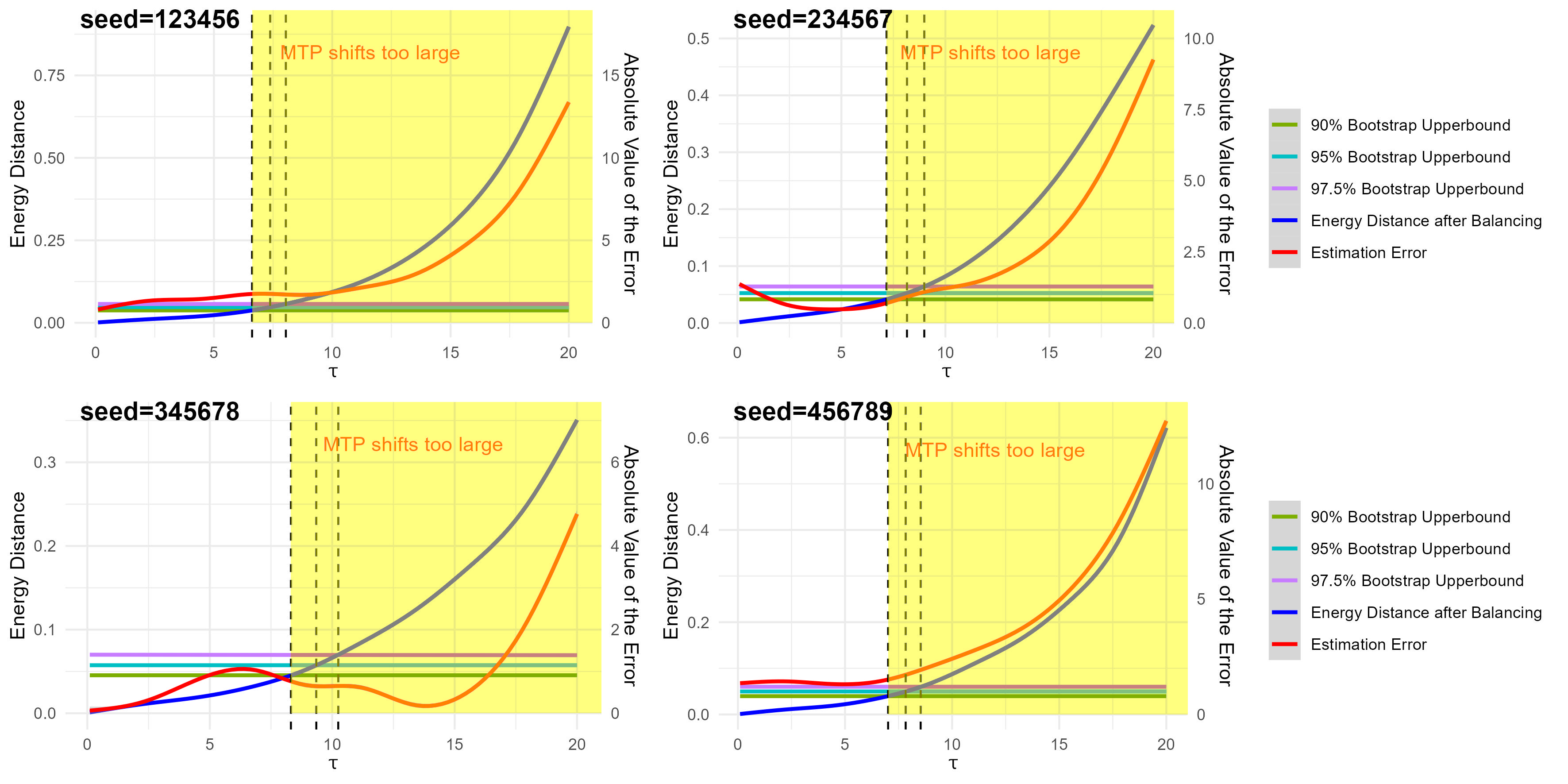
Figure 1: Four general scenarios that demonstrate our method for selecting a feasible MTP scale. The X-axis represents the MTP scale, with larger values of $\tau$ indicating greater shifts. The blue curve shows the energy distance after balancing, while the three horizontal lines represent the calculated thresholds. The MTP corresponding to the $\tau$ values, for which the weighted energy distance exceeds these thresholds, are considered to be MTP magnitudes with concern for uncontrolled measured confounding. The estimation error curve (red curve) validates our method, as its value appears to increase significantly when employing the danger MTP magnitudes.

Consider the null hypothesis that the weights from a given balancing method perfectly balance the observed population $\{{\boldsymbol{X}}_{i},A_{i}\}_{i=1}^{n}$ and the target population $\{{\boldsymbol{X}}_{i},q({\boldsymbol{X}}_{i},A_{i})\}_{i=1}^{n}$ for an MTP and thus completely control for measured confounding. The energy distance of the weighted empirical CDF $F_{n,{\boldsymbol{w}},{\boldsymbol{X}},A}$ and the target empirical CDF $F_{n,{\boldsymbol{X}},A}^{q}$ is nonzero only due to sampling variability. We can estimate the distribution of the energy statistic under this null hypothesis of no measured confounding to determine whether a given weighting method has balanced the weighted distribution to the target. We consider threshold values of this null distribution above which one may declare that the energy distance between a weighted distribution and the target shifted distribution is large enough that confounding is not plausibly controlled for. The threshold can be estimated through the following nonparametric bootstrap: For the $r=1,...,R$-th bootstrap iteration, obtain the bootstrap sample $\{{\boldsymbol{X}}_{i}^{r},A_{i}^{r}\}_{i=1}^{n}$ by sampling with replacement from the observed sample $\{{\boldsymbol{X}}_{i},A_{i}\}_{i=1}^{n}$ and calculating the corresponding bootstrap energy distance as $\mathcal{E}^{r}=\mathcal{E}(F_{n,{\boldsymbol{X}},A}^{rq},F_{n,{\boldsymbol{X}},A}^{q})$ where $F_{n,{\boldsymbol{X}},A}^{rq}$ is the empirical CDF for the bootstrap sample $\{{\boldsymbol{X}}_{i}^{r},q({\boldsymbol{X}}_{i}^{r},A_{i}^{r})\}_{i=1}^{n}$. The threshold can then be calculated as the one-sided upper $1-\alpha$ (typically 0.95) quantile of the bootstrap sample $\{\mathcal{E}^{r}\}_{r=1}^{R}$. If the energy distance is larger than the threshold, we may conclude that the weights do not balance the observed distribution to the target population under the given MTP $q({\boldsymbol{X}},A)$, indicating that the magnitude of the MTP is too large and thus must be reduced in order to obtain a reliable estimate. Note that the bootstrap threshold and the energy distance $\mathcal{E}(F_{n,{\boldsymbol{w}},{\boldsymbol{X}},A},F_{n,{\boldsymbol{X}},A}^{q})$ all depend on the choice of the MTP, so the bootstrap procedure must be run anew for each change to the MTP scale.

We illustrate this new approach through the example using our novel energy balancing weights (introduced in Sections 5 and 6). Simulated data are generated using the first condition of our simulation study described in Section 7 with $n=300$ and dimensionality $p=20$. For simplicity, we consider the monotone shift function $q({\boldsymbol{x}},a)$ where all interventions are shifted with the same value $\tau$: $q({\boldsymbol{x}},a)=a+\tau$ where $\tau$ ranges from $[0,20]$ in increments of 0.1. Larger values of $\tau$ represent the larger discrepancies from the original treatment. For each $\tau$, we calculate the weighted energy distance for the estimated energy balancing weights, the error of the energy balancing weights estimator, the $97.5\%$, $95\%$ and $90\%$ upper quantiles of the bootstrap null distribution (described above). Figure 1 displays four general scenarios with different random seeds. The energy distance for the energy balancing weights increases with a larger MTP scale $\tau$; along with this increase, the error of the estimator also increases monotonically. The three vertical dashed lines indicate the intersection of the energy distance and the three thresholds based on the upper quantiles of the null distribution. We can see that for $\tau$ value less than the vertical lines, the estimation error is generally controlled, indicating that this procedure is a reasonable criterion for choosing a feasible MTP scale.

4.2 Evaluation of arbitrary weights for a given MTP and dataset

The previous section evaluates different MTP scales with a fixed weighting method. Similarly, we can also use the weighted energy distance to evaluate the performance of different weights for a fixed MTP. Since smaller weighted energy distances indicate better balance between the weighted sample and the shifted sample, a natural criterion is to select the method that yields the smallest weighted energy distance. We demonstrate this approach to weight selection using the simulation results with sample sizes $n=800$ and covariate dimensionality $p=80$ under the first simulation scenario described in Section 7.

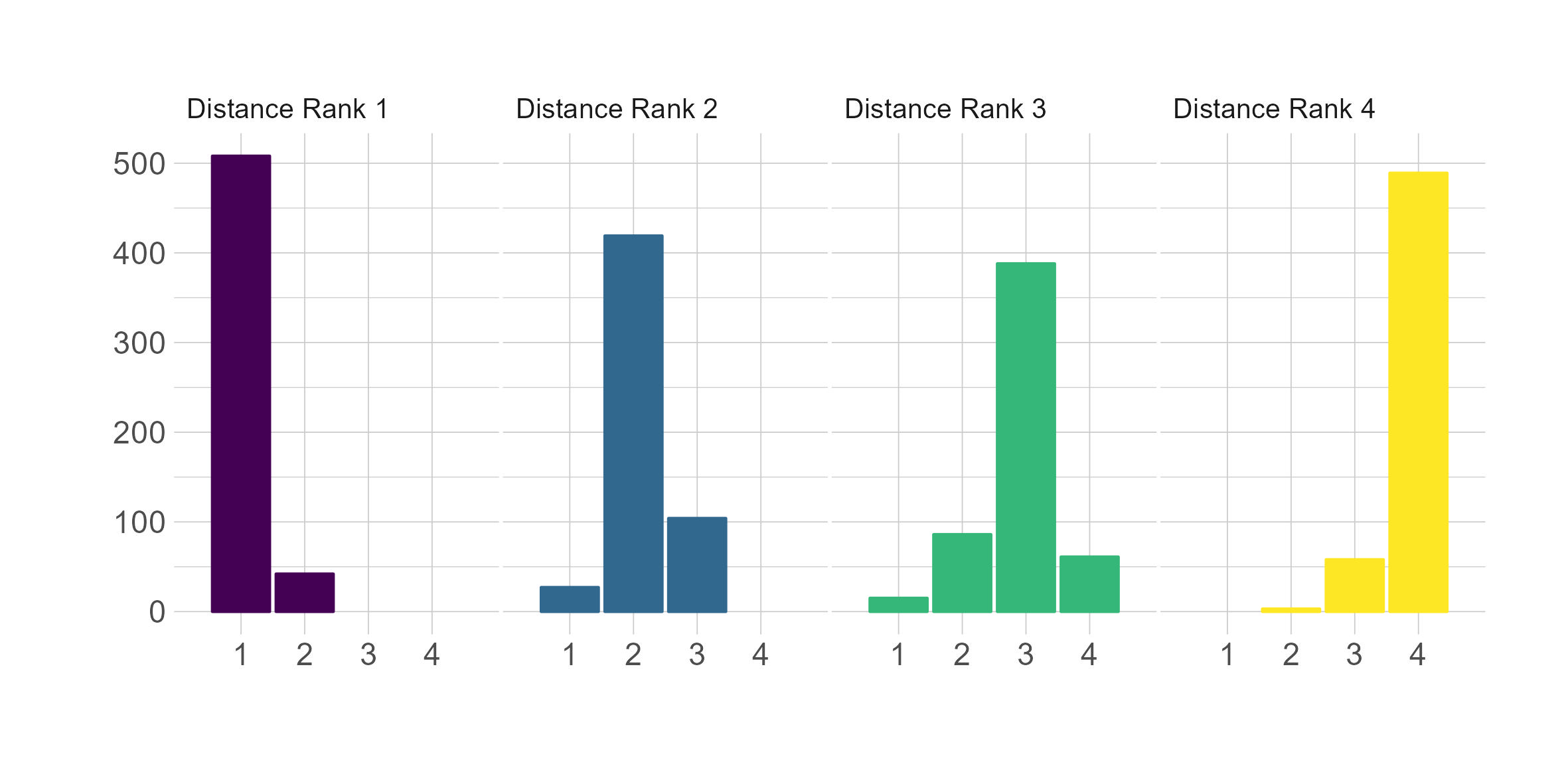
Figure 2: The histogram depicts the association between the rank of estimation error and the rank of weighted energy distance using the same data as in Figure 2. The x-axis of each plot is the rank of each method in terms of performance. The figure shows that, in most cases, the method with the lowest weighted energy distance yields the best performance.

Figure 2 displays the distribution of the rank of the absolute estimation error for a given dataset compared with the rank of the weighted energy distance for the four weighting methods. From this, the weighting method with the smallest energy distance (rank 1) tends to perform best in most cases. In Section 3 of the Supplementary Material, we further explore the validity of this method under broader conditions.

5 Energy balancing weights for MTP estimation

As demonstrated in the error decomposition in Section 2.2, weighted distributional imbalance is a critical component of the estimation bias of weighted estimators for MTPs. Further, we showed in Lemma 3.1 and Theorem 3.2 that the weighted energy distance characterizes weighted distributional imbalance. In this section we propose a new set of weights designed as the optimizer of this measure. By minimizing the distance between the weighted empirical distribution and target distribution, our proposed weights, which we call energy balancing weights (EBWs), control for confounding in a robust and flexible manner. Specifically, these weights minimize the energy distance between the observed sample (weighted empirical CDF) and the target sample under the MTP (MTP-shifted empirical CDF). Thus, the energy balancing weights balance the weighted empirical distribution to the MTP-shifted empirical distribution.

Extensively highlighted in the weighting literature, extreme weights can inflate the variance of the estimator (Li et al., 2018; Chattopadhyay et al., 2020). To ensure root-$n$ consistency of our energy balancing estimator, it is necessary to impose a restriction to avoid extreme weights. One approach is to introduce an additional penalization term for the sum of squared weights, resulting in penalized energy balancing weights. In this section, we introduce the penalized energy balancing weights ${\boldsymbol{w}}^{ep}_{n}$. Under mild conditions, we show these weights result in root-$n$ consistency in estimating the mean potential outcome under an MTP.

5.1 Penalized Energy Balancing Estimator

The penalized energy balancing weights account for the magnitude of the weights in addition to the weighted energy distance. Specifically, we define the penalized energy balancing weights ${\boldsymbol{w}}^{ep}_{n}$ with a user-specified parameter $\lambda>0$ as follows:

$$\begin{split}{\boldsymbol{w}}_{n}^{ep}&\in\underset{{\boldsymbol{w}}=(w_{1},...,w_{n})}{\arg\min}\mathcal{E}(F_{n,{\boldsymbol{w}},{\boldsymbol{X}},A},F_{n,{\boldsymbol{X}},A}^{q})+\frac{\lambda}{n^{2}}\sum_{i=1}^{n}w_{i}^{2}\textnormal{ s.t. }\sum_{i=1}^{n}w_{i}=n\,,w_{i}\geq 0.\end{split}$$ (12)

The corresponding penalized energy balancing estimator is then $\hat{\mu}^{q}_{{\boldsymbol{w}}^{ep}_{n}}=n^{-1}\sum_{i=1}^{n}{\boldsymbol{w}}_{i,n}^{ep}Y_{i}$. Analogous to Huling and Mak (2020), we prove the following properties of the energy balancing weights. Theorem 5.1 shows that the penalized energy balancing weights make the weighted empirical CDF of the observed data converge to the true MTP-shifted CDF.

Theorem 5.1.

Assume the assumptions in the previous theorems hold. Let $w_{n}^{ep}$ be the penalized energy balancing weights. Then, we have $\lim_{n\to\infty}F_{n,{\boldsymbol{w}}_{n}^{ep},{\boldsymbol{X}},A}({\boldsymbol{x}},a)=F_{{\boldsymbol{X}},A}^{q}({\boldsymbol{x}},a)$ almost surely for every continuity point $({\boldsymbol{x}},a)\in\mathcal{X}$. Furthermore, the following holds almost surely

$$\lim_{n\to\infty}\mathcal{E}(F_{n,{\boldsymbol{w}}_{n}^{ep},{\boldsymbol{X}},A},F_{n,{\boldsymbol{X}},A}^{q})=0.$$ (13)

We now show that the penalized energy balancing estimator achieves root-$n$ consistency.

Theorem 5.2.

Assume the conditions in Theorem 2. Let $\mathcal{H}$ be the native space induced by the radial kernel $\Phi(.)=-||.||_{2}$ on $(\mathcal{X},\mathcal{A})$. Suppose the following mild conditions hold:

• CP-1: $\mu(\cdot,\cdot)\in\mathcal{H}$

• CP-2: Var $[\mu({\boldsymbol{X}},A)]<\infty$

• CP-3: Var $[Y|X={\boldsymbol{x}},A=a]$ are bounded over $({\boldsymbol{x}},a)\in(\mathcal{X},\mathcal{A})$.

• CP-4: $\mathbb{E}[g^{2}({\boldsymbol{W}},{\boldsymbol{W}}^{\prime},{\boldsymbol{W}}^{\prime\prime},{\boldsymbol{W}}^{\prime\prime\prime})]\leq\infty$ where ${\boldsymbol{W}},{\boldsymbol{W}}^{\prime},{\boldsymbol{W}}^{\prime\prime},{\boldsymbol{W}}^{\prime\prime\prime}\stackrel{{\scriptstyle i.i.d.}}{{\sim}}F_{{\boldsymbol{X}},A}^{q}$ be a vector of $({\boldsymbol{X}},A)$ and, with $h({\boldsymbol{w}})=\frac{f^{q}_{{\boldsymbol{X}},A}({\boldsymbol{x}},a)}{f_{{\boldsymbol{X}},A}({\boldsymbol{x}},a)}$, the kernel function $g(.)$ is defined as:

  $$g({\boldsymbol{w}},{\boldsymbol{w}}^{\prime},{\boldsymbol{w}}^{\prime\prime},{\boldsymbol{w}}^{\prime\prime\prime})=h({\boldsymbol{w}})||{\boldsymbol{w}}-{\boldsymbol{w}}^{\prime\prime}||_{2}+h({\boldsymbol{w}}^{\prime})||{\boldsymbol{w}}^{\prime}-{\boldsymbol{w}}^{\prime\prime\prime}||_{2}-h({\boldsymbol{w}})h({\boldsymbol{w}}^{\prime})||{\boldsymbol{w}}-{\boldsymbol{w}}^{\prime}||_{2}-||{\boldsymbol{w}}^{\prime\prime\prime}-{\boldsymbol{w}}^{\prime\prime}||_{2}$$

Then, the proposed penalized EBW estimator $\hat{\mu}_{q,{\boldsymbol{w}}_{n}^{ep}}$ is root-$n$ consistent in that

$$\sqrt{\mathbb{E}_{{\boldsymbol{X}},A,Y}[(\hat{\mu}^{q}_{{\boldsymbol{w}}^{ep}_{n}}-\mu^{q})^{2}]}={O}_{p}(n^{-1/2}).$$ (14)

Theorem 5.2 shows that the penalized energy balancing weights yield a root-$n$ consistent estimate of $\mu^{q}$ under mild conditions on the data-generating process even though the energy balancing weights are not shown to be consistent for the true density ratio weights in any sense.

We briefly comment on the conditions required for Theorem 5.2. Condition CP-1 requires that the outcome regression function be contained in the native space $\mathcal{H}$. As demonstrated in Huling and Mak (2020), this condition is a smoothness assumption on the true outcome regression function $\mu({\boldsymbol{x}},a)$. CP-2 requires that the outcome regression function have finite variance and CP-3 requires that the conditional variance function be bounded. These two conditions are both mild and fairly weak in practice. CP-4 is a requirement that certain moments of the covariates and treatments be bounded.

6 Augmented Energy Balancing Estimator

Augmented estimator is a widely-used approach in the causal inference literature that combine balancing weights and an estimated outcome model to improve the estimation of a causal effect, potentially increasing efficiency and reducing sensitivity to model misspecification. In this context, we propose an augmented version of the energy balancing estimator that incorporates an estimated outcome model. Because the energy balancing weights were shown to yield consistent estimates of $\mu^{q}$ without the need for an outcome regression model, this allows the analyst to utilize an outcome regression model primarily for the purpose of variance reduction.

Let $\hat{\mu}({\boldsymbol{x}},a)$ be an estimate of the outcome regression function $\mu({\boldsymbol{x}},a)$. The augmented estimator is constructed by subtracting $\int_{\mathcal{X}}\int_{\mathcal{A}}\hat{\mu}({\boldsymbol{x}},a)d(F^{q}_{n,{\boldsymbol{X}},A}-F_{n,{\boldsymbol{w}}^{e}_{n},{\boldsymbol{X}},A})({\boldsymbol{x}},a)$ from the weighted estimator $\hat{\mu}_{{\boldsymbol{w}}_{n}^{ep}}^{q}=\sum_{i=1}^{n}w_{i}^{ep}Y_{i}$. The resulting augmented energy balancing estimator is

$$\begin{split}\hat{\mu}_{AG}^{q}&=\hat{\mu}_{{\boldsymbol{w}}_{n}^{ep}}^{q}-\int_{\mathcal{X}}\int_{\mathcal{A}}\hat{\mu}({\boldsymbol{x}},a)d(F^{q}_{n,{\boldsymbol{X}},A}-F_{n,w^{ep}_{n},{\boldsymbol{X}},A})({\boldsymbol{x}},a)\\ &=\frac{1}{n}\sum_{i=1}^{n}w^{ep}_{i}(Y_{i}-\hat{\mu}({\boldsymbol{X}}_{i},A_{i}))+\frac{1}{n}\sum_{i=1}^{n}\sum_{j=1}^{J({\boldsymbol{X}}_{i})}I_{j,{\boldsymbol{X}}_{i}}(A_{i})\hat{\mu}({\boldsymbol{X}}_{i},q_{j}({\boldsymbol{X}}_{i},A_{i})).\end{split}$$ (15)

In the second form, the weighted residuals can be view as a bias correction term for the outcome regression-based estimate of the MTP effect. We show its asymptotic normality and propose a statistically-valid and computationally-efficient multiplier bootstrap for inference.

6.1 Asymptotic normality

In this section we demonstrate the asymptotic distribution of augmented energy balancing estimator $\hat{\mu}_{AG}^{q}$. The required conditions for asymptotic normality are:

• CA-1: $\hat{\mu}({\boldsymbol{x}},a)$ is such that $\hat{\mu}-\mu\in\mathcal{H}$.

• CA-2: ${\boldsymbol{w}}^{e}_{n}$ satisfy $1\leq{\boldsymbol{w}}_{i}^{e}\leq BN^{1/3}$ for some constant $B$.

• CA-3: $\max_{i}E(|\epsilon_{i}|^{3})<\infty$ for each $n$.

• CA-4: $\hat{\mu}({\boldsymbol{x}},a)$ is a consistent estimator of $\mu({\boldsymbol{x}},a)$.

Condition CA-1 requires that the outcome regression model minus the true outcome regression model be contained in the native space $\mathcal{H}$. This condition somewhat limits the complexity of the error function of the estimated outcome regression model. Condition CA-2 has been used before in the literature; see Athey et al. (2016); Huling et al. (2023). This condition can be imposed directly in the weight optimization procedure without changing the empirical performance of the weights or any of the asymptotic results of the weights, as in Huling et al. (2023). Condition CA-3 indicates that the error term has finite third moments, and condition CA-4 requires consistency of the outcome regression model; CA-4 is only required for studying the asymptotic distribution of $\hat{\mu}^{q}_{AG}$ and is not needed to show consistency or the convergence rate of $\hat{\mu}^{q}_{AG}$ for $\mu^{q}$. With these conditions, we have the following:

Theorem 6.1.

Under Conditions C1-C4, let $J_{n}=n^{1/2}(\hat{\mu}_{AG}^{q}-\mu^{q})$ and $J_{n}^{*}=[Var(\mu({\boldsymbol{X}},A))]^{1/2}F+\sigma n^{-1/2}\sum_{j=1}^{n}w_{j}^{e}G_{j}$ where $F,G_{1},...,G_{n}$ are independently and identically distributed standard normal random variables independent of ${\boldsymbol{X}}_{1},...,{\boldsymbol{X}}_{n},A_{1},...,A_{n}$ and $\epsilon_{1},...,\epsilon_{n}$. Let $\psi_{n}$ and $\psi_{n}^{*}$ be the corresponding characteristic functions of $J_{n}$ and $J_{n}^{*}$. Then as $n\to\infty$, $|\psi_{n}(t)-\psi_{n}^{*}(t)|\to 0,t\in\mathbb{R}$ where $\psi_{n}^{*}(t)$ is twice differentiable, and

$$\limsup_{n}\mbox{Var}(J_{n})\leq\mbox{Var}(\mu({\boldsymbol{X}},Q))+\sigma^{2}V,$$ (16)

where $\mu({\boldsymbol{X}},Q)=\sum_{j=1}^{J(X)}I_{j,{\boldsymbol{X}}}(A)\mu({\boldsymbol{X}},q_{j}({\boldsymbol{X}},A))$ is the conditional mean under the MTP and $V=\mbox{E}\left(\frac{f^{q}_{{\boldsymbol{X}},A}({\boldsymbol{X}},A)}{f_{{\boldsymbol{X}},A}({\boldsymbol{X}},A)}\right)^{2}+D$ is the variance of the Radon-Nikodym weights plus a positive number.

Theorem 6.1 demonstrates that the energy balancing weights, when paired with a consistent outcome regression model, achieve asymptotic normality and may be efficient, however, an exploration of the conditions under which efficiency is guaranteed requires additional exploration.

6.2 Inference

The asymptotic normality of our augmented estimator $\hat{\mu}_{AG}^{q}$ allows us to use a standard bootstrap method to estimate its uncertainty and conduct statistical inference for the estimator. However, in practice, the standard nonparametric bootstrap method has some limitations. First, it can be computationally intensive because both the penalized energy balancing weights and the outcome regression estimator must be re-computed during each bootstrap iteration $r=1,...,R$. This can be especially time-consuming for large values of $R$ (e.g., $R=10000$). Further, in some extreme resamples, it may exacerbate issues of overlap by chance.

We thus propose a multiplier bootstrap method originally presented by Wu (1986) that allows for quick computation. Similar to Matsouaka et al. (2023) (which they name a wild bootstrap), the method perturbs the influence function of the estimator to estimate its variance. The influence function for our augmented estimator is

$$\varphi_{i}=\frac{f^{q}_{{\boldsymbol{X}},A}({\boldsymbol{X}},A)}{f_{{\boldsymbol{X}},A}({\boldsymbol{X}},A)}(Y_{i}-\mu({\boldsymbol{X}}_{i},A_{i}))+\sum_{i=1}^{J({\boldsymbol{X}}_{i})}I_{j,{\boldsymbol{X}}_{i}}(A_{i})\mu({\boldsymbol{X}}_{i},q_{j}({\boldsymbol{X}}_{i},A_{i}))-\mu^{q}.$$

We estimate the influence function by plugging in the estimators $\hat{\mu}^{q}$, $\hat{\mu}({\boldsymbol{X}},A)$, and $w_{i}^{ep}$ for their population counterparts:

$$\hat{\varphi}_{i}=w_{i}^{ep}(Y_{i}-\hat{\mu}({\boldsymbol{X}}_{i},A_{i}))+\sum_{i=1}^{J({\boldsymbol{X}}_{i})}I_{j,{\boldsymbol{X}}_{i}}(A_{i})\hat{\mu}({\boldsymbol{X}}_{i},q_{j}({\boldsymbol{X}}_{i},A_{i}))-\hat{\mu}^{q}.$$ (17)

Even though $w_{i}^{ep}$ does not necessarily estimate the true inverse propensity score, we show that the following procedure is still valid. Then, the multiplier bootstrap estimator $\hat{\Sigma}$ can be constructed as displayed in Algorithm 1. A $95\%$ Wald-type confidence interval of $\hat{\mu}_{AG}^{q}$ can be calculated as $\hat{\mu}_{AG}^{q}\pm 1.96\times n^{-1/2}\hat{\Sigma}^{1/2}$.

Algorithm 1 Multiplier bootstrap

1:for $r=1,...,R$-th bootstrap iteration do

2:     Generate random variable $\xi=(\xi_{1},...,\xi_{n})$ with $\xi_{i}\sim\exp(1)$ for $i=1,...,n$.

3:     Compute $\hat{q}^{q}_{r}=\frac{1}{\sqrt{n}}\sum_{i=1}^{n}\xi_{i}\hat{\varphi}_{i}$

4:end for

5:Calculate $\hat{\Sigma}^{1/2}=$IQR$(\hat{q}^{q})/(z_{0.75}-z_{0.25})$ where IQR$(\hat{q}^{q})$ is the interquartile range of $\{\hat{q}^{q}_{r}\}_{r=1}^{R}$ and $z_{0.75}-z_{0.25}=1.349$ be the interquartile range of standard normal distribution.

Here, we prove the validity of the proposed multiplier bootstrap in the following theorem.

Theorem 6.2.

We have that $\hat{q}^{q}_{r}=\frac{1}{\sqrt{n}}\sum_{i=1}^{n}\xi_{i}\hat{\varphi}_{i}\to n^{1/2}(\hat{\mu}_{AG}^{q}-\mu^{q})$ as $n\to\infty$.

Thus, Theorem 6.2 shows that one can estimate the asymptotic distribution of $\hat{\mu}^{q}_{AG}$ using the multiplier bootstrap procedure in Algorithm 1. An advantage of the multiplier bootstrap procedure over the standard bootstrap is that the weights and outcome regression model only need to be estimated once, not $R$ times. This results in a substantial computational speedup for most applications, as demonstrated in the next section.

7 Simulation studies

In this section, we study the empirical properties of the proposed energy balancing weights and further to assess their relative performance to other commonly used estimators for MTPs. The aim of the simulation study is to evaluate the performance of our proposed estimators under different simulation conditions. Comparator methods include the clever classification method proposed in D\́boldsymbol{i}az et al. (2021), density ratio (IPW) with estimated generalized propensity score, and the targeted minimum-loss based estimator (TMLE) (D\́boldsymbol{i}az et al., 2021) implemented in the R package lmtp (Williams and D\́boldsymbol{i}az, 2023) that utilizes both a density ratio estimator and an outcome regression model. These methods will be further described in the following subsection.

7.1 Data generating mechanisms

We have two main simulation conditions: a moderately complex data-generating mechanism (simulation study # 1) and a highly complex (simulation study # 2) data-generating mechanism. For each simulation setting, we vary the following settings: the sample size $(n=100,200,400,800)$, the number of covariates $(p=10,20,40,80)$ for each individual, and the treatment type. This allows us to inspect the joint effects of dimensionality and increasing sample size on the empirical performance of all methods. We replicate all simulation experiments under two different conditions on the treatment variable: one condition where the treatment is continuously-distributed, and the other where the treatment has discrete, but countably infinite, support. Here, we briefly illustrate the data-generating mechanism. Readers are referred to Section 5.1 of the Supplementary Material for a detailed description of the data-generating mechanism. 1) The covariates are generated randomly following either a uniform distribution or a binomial distribution. 2) The treatment mean for a participant follows a cubic function of the covariates. 3) The moderately complex simulation condition assumes the outcome is a function of a quadratic term of the treatment times a cubic term of the covariates. The highly complex simulation condition further assumes interaction terms of the covariates. 4) The MTP function $q$ shifts the treatment more aggressively when the observed treatment is small. We emphasize that the estimation error (i.e., the observed sample mean effect minus the true MTP effect) is designed to be relatively stable with the increase of the number of covariates $p$, so that the complexity of the data-generating processes does not explode with dimension.

7.2 Estimands and estimators under evaluation

In each simulation replication, the estimand of interest is the mean potential outcome under the MTP. We evaluate three proposed energy balancing weight methods, including the penalized energy balancing weights described in Section 5.1, an unpenalized version of the energy balancing weights, and a kernelized energy balancing weights approach using the Gaussian kernel (see Supplementary Material Section 2). Various alternative estimators for balancing weights are considered, such as the naive, unadjusted method that assigns equal weights to all subjects, density ratio weights (IPW) with generalized propensity score estimated using a Poisson density (for the discrete intervention settings), and the classification method proposed by (D\́boldsymbol{i}az et al. (2021) Section 5.4) with classification models estimated by either 1) logistic regression or 2) a random forest. The corresponding augmented estimators for each weighting method are implemented using the same outcome model, the ensemble method SuperLearner (Van der Laan et al., 2007), which incorporates the eXtreme Gradient Boosting method Friedman et al. (2000) (SL.xgboost), lasso regularized generalized linear models (SL.glmnet), and a random forest model (SL.ranger). Also included is a targeted minimum-loss based estimator (TMLE) method (D\́boldsymbol{i}az et al., 2021) with all nuisance parameters estimated using SuperLearner.

7.3 Simulation results

In every simulation scenario, the true causal effect is determined using Monte Carlo with a sample size of 100,000. For each simulation setting, we repeat the experiment independently 1,000 times, applying each comparator method, allowing for the calculation of the mean squared error (MSE), bias, and coverage rate for 95% confidence intervals. The coverage rate is calculated based on Wald-type intervals with SE for each estimator estimated by the non-parametric bootstrap with 100 replications. Additionally, we also use the multiplier bootstrap method proposed in Section 6.2 for the augmented energy balancing estimator. The simulation results are displayed in Figures 3 and 4. Since the results of the two simulation studies are similar, we only display the MSE and coverage rate for the 95% confidence interval for the first simulation study. Readers can refer to Supplementary Material for the results for the highly complex setting.

In all simulation conditions, our three energy balancing methods (energy balancing, penalized energy balancing, and kernel energy balancing method) consistently outperform other methods in terms of both the bias and the coverage rate, indicating their robustness and ability to handle various situations. This pattern holds both for pure weighting (not augmented) estimators and for augmented estimators, however, the non-augmented energy balancing estimators work best of all in most settings. The penalized energy balancing weights exhibit slightly worse performance in terms of bias compared to the energy balancing weights, which is probably due to the additional penalty term in the estimation. The kernel energy balancing weights (using the MMD described in the Supplementary Material Section 2.2) have the smallest bias in most cases when the sample size is relatively small; however, their performance varies significantly among different conditions and the bias does not improve as much with the increase of the sample sizes. This unstable performance may be due to the choice of bandwidth parameters in the Gaussian kernel function, which is the median heuristic that is known to not necessarily perform well in all scenarios. Therefore, although we believe the kernel energy balancing method has the potential to be very flexible and perform well in practice, its performance may depend critically on the choice of tuning parameters. Consequently, we recommend using penalized energy balancing methods that are more stable across different conditions.

The augmented energy balancing estimator does not perform as well as the three energy balancing estimators, possibly because the outcome model dominates the empirical performance of the method in the particular simulation settings we investigated using the outcome modeling approach we used throughout. We note that our outcome regression model, while flexible, struggles to model the outcome regression function well; a more suitable outcome model would likely yield better performance for the augmented estimators. In fact, all the augmented estimators exhibit similar performance in terms of bias, which we believe primarily reflects the performance of the fitted outcome model rather than the weights. Further studies are necessary to gain a better understanding of this phenomenon.

The coverage rate results (Figure 4) align with our observations for bias and MSE. All three energy balancing methods exhibit good coverage rate performance. Owing to its small bias, the coverage rate for the kernel energy balancing method approaches 95% most closely. For the moderately complex simulation condition (simulation study #1), most augmented methods achieve reasonable coverage with 800 sample sizes. However, their coverage remains quite low when the data-generating mechanism becomes more complex (see the supplementary material Figure 5) as the bias induced by the misspecified outcome regression models seems to have an ill-effect on their coverage. This further highlights the robustness of our methods in handling various practical conditions. It is worth emphasizing the similar performance of the multiplier bootstrap and the non-parametric bootstrap for the augmented energy balancing method. The convergence of the results validates the use of the multiplier bootstrap as a more efficient way to calculate the uncertainty of the augmented energy balancing estimator.

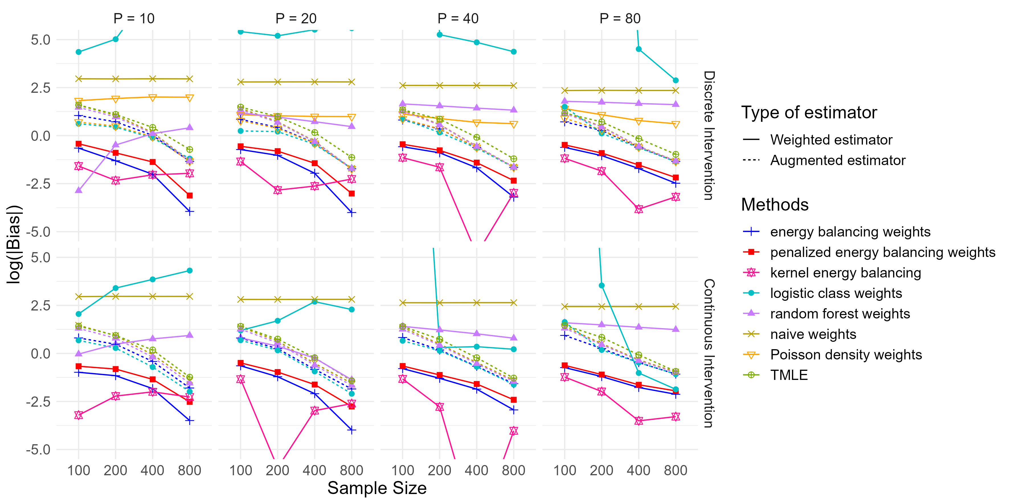
Figure 3: Simulation results in terms of the logarithm of the absolute value of bias across different sample sizes, type of treatment/intervention variable, and the dimensionality of covariates. The data-generating mechanism is moderately complex (simulation # 1). Balancing methods are displayed in different colors and shapes of points. Weighted estimators are displayed in solid lines and the augmented estimators are in dashed lines.

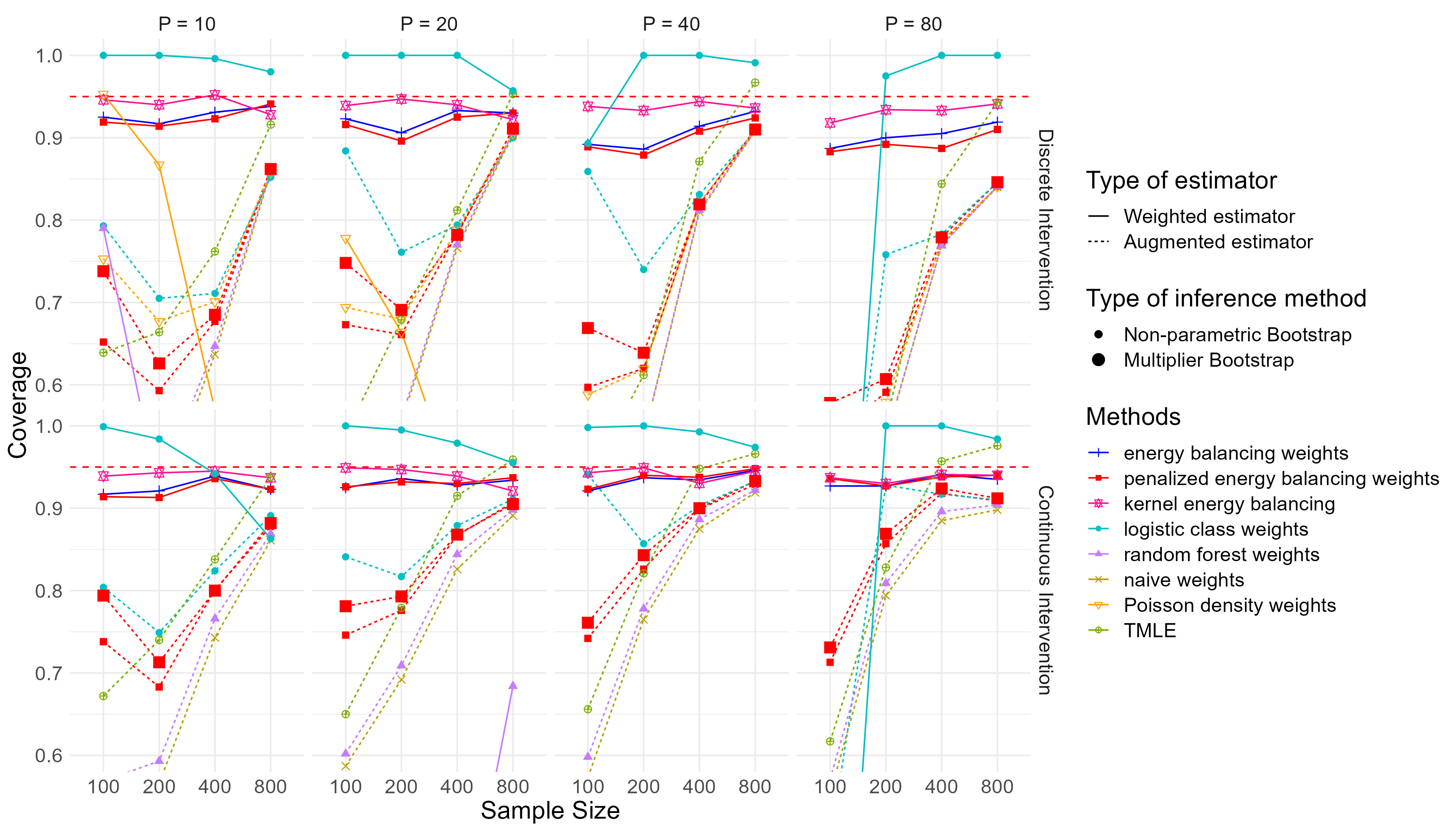
Figure 4: Simulation result for the 95% coverage rate across different sample sizes and dimensionality of covariates. The data-generating mechanism is moderately complex (simulation # 1). The red dashed line indicates nominal 95% coverage. Different weighting methods are displayed in different colors and shapes of points. Weighted estimators are displayed in solid lines and the augmented estimators are in dashed lines. The multiplier bootstrap method is displayed in a larger size of the red points.

8 Case Study: Mechanical Power of Ventilation

Critically ill patients often require mechanical ventilation to support their breathing. The ventilator delivers a controlled amount of air (tidal volume) at a specific pressure and rate to ensure adequate gas exchange in the lungs. In order to overcome the resistance of the airway and expand the thorax wall, the ventilator needs to transfer a certain amount of energy to the patient’s respiratory system (Neto et al., 2018, 2016; Cressoni et al., 2016). Mechanical power (MP) is a comprehensive parameter that quantifies the amount of energy transferred to the patient’s respiratory system during each breath. It takes into account tidal volume, respiratory rate, peak airway pressure, and positive end-expiratory pressure (PEEP) (Gattinoni et al., 2016). Excessive ventilatory settings can result in ventilator-induced lung injury (VILI), which can worsen the patient’s clinical condition and increase the risk of mortality (Neto et al., 2016; Cressoni et al., 2016). Previous research has suggested that factors like high tidal volume, high airway pressures, and high respiratory rates could be associated with an increased risk of lung injury and poor outcomes (Nieman et al., 2016). However, these individual factors do not capture the overall impact of ventilation settings on the lungs. Mechanical power can provide a more comprehensive assessment of the risk associated with different ventilatory settings.

A recent study (Neto et al., 2018) examined data from the high-resolution databases of the Medical Information Mart for Intensive Case (MIMIC)-III (Johnson et al., 2016) and the eICU Collaborative Research Database (eICU) (Goldberger et al., 2000). These databases contain information on critically ill patients who required mechanical ventilation in the intensive care unit (ICU). All included patients received invasive ventilation for at least 48 consecutive hours. Time-varying variables were collected at 8-hour intervals for the entire 48-hour period. (Neto et al., 2018) defined the exposure as the mean between the highest and lowest value of MP in the second 24 hours and concluded that high MP is independently associated with higher in-hospital mortality. In this case study, we reanalyze the dataset from Neto et al. (2018) to explore the causal relationship between a postulated MTP of MP and in-hospital mortality.

We excluded patients with zero MP in Joules/min or extreme MP values (MP greater than 150 Joules/min) from the analysis. The exposure of interest is the mean value between the highest and lowest MP during the second 24 hours. The potential confounding variables we aim to balance are measured during or prior to the first 24 hours. As in Neto et al. (2018), our primary focus is on the in-hospital mortality of the included participants. The dataset contains a total of 5,011 participants with 97 identified covariates; among these covariates are many of the important factors such as the PaO2/FiO2 Ratio that are used in guidelines for determining mechanical ventilator settings. We use the following MTP to explore the causal effect of MTP that decreases the MP value based on its original value. This MTP reduces MP for individuals with high MP more aggressively, as earlier studies have indicated potential harms of high MP. The shifted MP value $q({\boldsymbol{x}},a)$ is defined as $q({\boldsymbol{x}},a)=a$ if $0<a<5$, $q({\boldsymbol{x}},a)=a-5\tau$ if $5<a<10$, $q({\boldsymbol{x}},a)=a-10\tau$ if $10<a<20$, $q({\boldsymbol{x}},a)=a-15\tau$ if $20<a<40$, $q({\boldsymbol{x}},a)=a-30\tau$ if $40<a$. Here $a$ is the original MP value and $\tau$ is the parameter that controls the magnitude of the MTP (a larger value of $\tau$ results in a more dramatic decrease of MP).

With the $\tau$ ranging from 0 to 1 for the MTPs, our analysis is displayed in Figure 5. For each value of $\tau$, the top axis displays the mean value of MP under the corresponding MTP. To identify a range of the shift magnitude $\tau$ for which confounding control via our energy balancing weights is feasible, we calculate the sampling variation of the energy distance under the corresponding MTP as described in Section 4.1. The upper 90%, 95%, and 97.5% percentiles of the bootstrap sample are plotted with smoothed lines in the figure. Again, these values represent the intrinsic tails of variation of the energy distance when the two distributions are identical (i.e., the population is perfectly balanced). If the actual energy distance after balancing is larger than these upper bounds, the validity of the hypothesis that the population is balanced after weighting becomes questionable. The energy distance between the weighted sample and the target sample under the MTP is displayed as the blue curve for each value of $\tau$. From the results, MTPs with $\tau$ larger than 0.9 have an energy distance which reaches the upper 90% threshold, which indicates moderately poor balance of the covariates under the corresponding MTP shifts after weighting and thus any analysis results have the potential of confounding bias. Values of $\tau$ ranging from 0 to 0.75 have smaller energy distances after weighting, indicating that the shifts are within a reasonable range and have low risk of bias due to measured confounding.

The estimated potential in-hospital mortality rate under the MTP and the corresponding 95% confidence interval are displayed in Figure 5. Within the range of $\tau$ that has low risk of confounding bias, the expected potential mortality under the MTP monotonically decreases with larger values of $\tau$ (i.e., a larger decrease of MP). When $\tau>0.29$, the estimated upper bound of the 95% confidence interval of the mortality rate is smaller than the average mortality rate of the sample which indicates that reducing MP via the defined MTP would significantly reduce in-hospital mortality. Note that when $\tau=0.29$, the energy distance after balancing is very close to 0 and the average MP after shifting decreases from 20 to 16.5 Joules/min. These observations suggest that measured confounding after weighting is not a major issue, which strengthens the validity of the significant result that a lower MP than used in practice would likely decrease in-hospital mortality. Compared to the results from (Neto et al., 2018; Hong et al., 2021), we adopted an MTP analysis, which strengthens the evidence about the potential harms of high MP due to the weakened assumptions that our MTP estimators operate under.

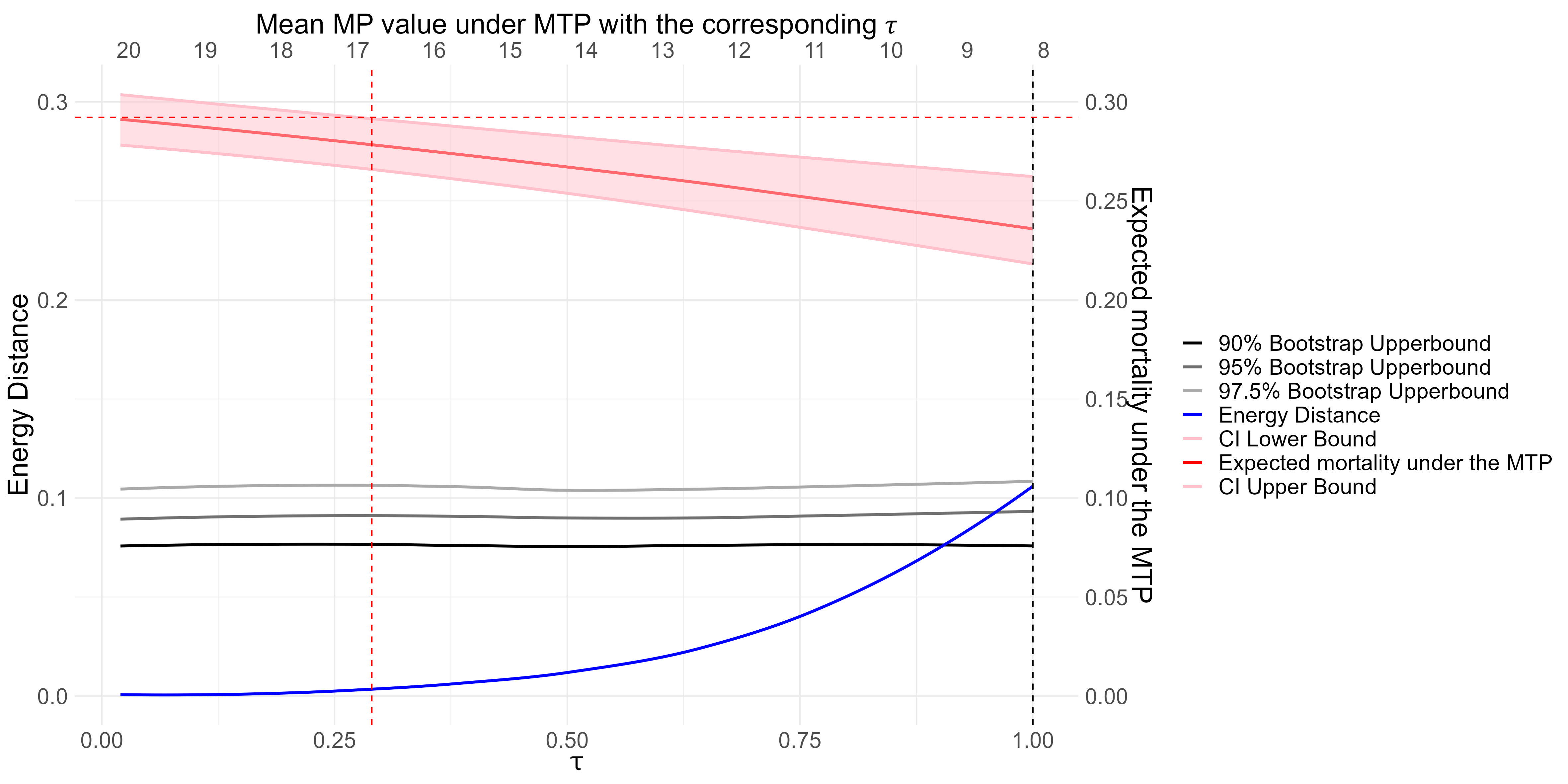
Figure 5: Exploring different magnitudes of MTP shifts to mechanical power of ventilation. The X-axis represents the $\tau$ value which controls the amount of the MTP shift. For each MTP shift, the blue curve displays the energy distance of the penalized energy balancing weights described in section 5. The three grey lines represent the 90%, 95%, and 97.5% threshold for the upper limit of energy distance, which are estimated using the bootstrap method described in Section 4.1. The red curve along with the shaded area is the estimated mortality and its 95% CI with the corresponding MTP.

9 Discussion

Estimating causal effects of treatments from observational data is particularly challenging due to confounding. This issue is further compounded when the treatment takes continuous values. An MTP analysis is well-suited for this scenario and defines a hypothetical intervention on a treatment variable based on the baseline characteristics and the observed treatment value. However, the choice of the hypothetical intervention in an MTP is still subjective and it faces the dilemma that, 1) if the definition of MTP is too conservative (i.e., the shift of the intervention is very small), the causal effect of the MTP may be too small to have material clinical implications and on the other hand 2) if the definition of MTP is too aggressive, then the observed population and the population under MTP will be intrinsically different, which makes confounding a major issue again, negating many of the conceptual and practical benefits of MTPs. There is a lack of methods that can measure the magnitude of the potential for measured confounding and help to define a reasonable MTP that can be reliably estimated from the data at hand.

In this paper, we demonstrate the connection between the estimation bias of weighted estimators of the causal effect under an MTP and weighted distributional imbalance. By explicitly defining the target population under MTP, we propose an error decomposition that highlights the role of covariate balance as a critical component of the estimation bias. We then introduce a distance, based on the weighted energy distance of Huling and Mak (2020), that explicitly characterizes this imbalance. As a result, the performance of any arbitrary set of weights in controlling for confounding for MTPs can be gauged through the weighted energy distance. Two methods are proposed to enhance the estimation of MTP effects: 1) we propose a method for assessing the performance of various balancing weights according to their weighted energy distance; this approach enables researchers to choose different balancing techniques suitable for specific datasets, 2) we then propose a method to detect whether the MTP shift is too large for a balancing method. We use a bootstrap to measure the variability of the energy distance under the null hypothesis of no measured confounding. Comparing this with the energy distance after applying the balancing weights enables an assessment of whether the weights can effectively balance the covariates under the current MTP and thereby control for measured confounding. This comparison also sheds light on the extent of confounding challenges associated with an MTP paired with a given dataset.

Our second contribution is a novel covariate balancing weight method based on the energy distance. These energy balancing weights are generated by minimizing the weighted energy distance, thereby minimizing a measure of distributional imbalance and thus potential for bias. We additionally propose an augmented energy balancing estimator that integrates an outcome model with the balancing weights to help further reduce variance in the estimates. We establish the validity of our methods by demonstrating the root-$n$ consistency of these estimators and further asymptotic normality of the augmented estimator. Through simulation studies involving both moderately complex and highly complex scenarios, we showcase the stability and performance of our methods in terms of bias, mean squared error (MSE), and coverage rate across various conditions, reflecting their capacity to handle diverse real-world situations.

We further proposed a multiplier bootstrap method to estimate the uncertainty of the augmented energy balancing estimator. The multiplier bootstrap approach offers a more computationally efficient means for statistical inference compared to the classical nonparametric bootstrap, as it does not require calculating weights within each bootstrap iteration. We prove the large-sample properties of this multiplier bootstrap and, through simulation, illustrate its similarity to the nonparametric bootstrap in terms of the coverage rates.

There remain some statistical properties that warrant further exploration. The first is to show whether the energy balancing weights converge to the true density ratio, as doing so may enable clearer studies of the potential efficiency of our proposed estimators. Secondly, as suggested in the simulation study, the coverage rate for the energy balancing estimator and the penalized energy balancing estimator is approximately 95%, implying that both estimators exhibit asymptotic normal distribution. However, establishing the asymptotic distribution for the estimators using EBWs and penalized EBWs is highly challenging. Moreover, our methods can be extended by incorporating alternative distance measures in the estimation of energy balancing weights and studying their corresponding statistical properties.

References

- (1)
- Athey et al. (2016) Athey, S., Imbens, G. W., Wager, S. et al. (2016), Efficient inference of average treatment effects in high dimensions via approximate residual balancing, Technical report.
- Chattopadhyay et al. (2020) Chattopadhyay, A., Hase, C. H. and Zubizarreta, J. R. (2020), ‘Balancing vs modeling approaches to weighting in practice’, Statistics in Medicine 39(24), 3227–3254.
- Cressoni et al. (2016) Cressoni, M., Gotti, M., Chiurazzi, C., Massari, D., Algieri, I., Amini, M., Cammaroto, A., Brioni, M., Montaruli, C., Nikolla, K. et al. (2016), ‘Mechanical power and development of ventilator-induced lung injury’, Anesthesiology 124(5), 1100–1108.
- D\́boldsymbol{i}az and Hejazi (2020) D\́boldsymbol{i}az, I. and Hejazi, N. S. (2020), ‘Causal mediation analysis for stochastic interventions’, Journal of the Royal Statistical Society Series B: Statistical Methodology 82(3), 661–683.
- D\́boldsymbol{i}az and van der Laan (2013) D\́boldsymbol{i}az, I. and van der Laan, M. J. (2013), ‘Targeted data adaptive estimation of the causal dose–response curve’, Journal of Causal Inference 1(2), 171–192.
- D\́boldsymbol{i}az et al. (2021) D\́boldsymbol{i}az, I., Williams, N., Hoffman, K. L. and Schenck, E. J. (2021), ‘Nonparametric causal effects based on longitudinal modified treatment policies’, Journal of the American Statistical Association pp. 1–16.
- Friedman et al. (2000) Friedman, J., Hastie, T. and Tibshirani, R. (2000), ‘Additive logistic regression: a statistical view of boosting (with discussion and a rejoinder by the authors)’, The Annals of Statistics 28(2), 337–407.
- Gattinoni et al. (2016) Gattinoni, L., Tonetti, T., Cressoni, M., Cadringher, P., Herrmann, P., Moerer, O., Protti, A., Gotti, M., Chiurazzi, C., Carlesso, E. et al. (2016), ‘Ventilator-related causes of lung injury: the mechanical power’, Intensive Care Medicine 42, 1567–1575.
- Goldberger et al. (2000) Goldberger, A. L., Amaral, L. A., Glass, L., Hausdorff, J. M., Ivanov, P. C., Mark, R. G., Mietus, J. E., Moody, G. B., Peng, C.-K. and Stanley, H. E. (2000), ‘Physiobank, physiotoolkit, and physionet: components of a new research resource for complex physiologic signals’, Circulation 101(23), e215–e220.
- Hainmueller (2012) Hainmueller, J. (2012), ‘Entropy balancing for causal effects: A multivariate reweighting method to produce balanced samples in observational studies’, Political Analysis 20(1), 25–46.
- Haneuse and Rotnitzky (2013) Haneuse, S. and Rotnitzky, A. (2013), ‘Estimation of the effect of interventions that modify the received treatment’, Statistics in Medicine 32(30), 5260–5277.
- Hong et al. (2021) Hong, Y., Chen, L., Pan, Q., Ge, H., Xing, L. and Zhang, Z. (2021), ‘Individualized mechanical power-based ventilation strategy for acute respiratory failure formalized by finite mixture modeling and dynamic treatment regimen’, EClinicalMedicine 36.
- Huling et al. (2023) Huling, J. D., Greifer, N. and Chen, G. (2023), ‘Independence weights for causal inference with continuous treatments’, Journal of the American Statistical Association (just-accepted), 1–25.
- Huling and Mak (2020) Huling, J. D. and Mak, S. (2020), ‘Energy balancing of covariate distributions’, arXiv preprint arXiv:2004.13962 .
- Imai and Ratkovic (2014) Imai, K. and Ratkovic, M. (2014), ‘Covariate balancing propensity score’, Journal of the Royal Statistical Society: Series B (Statistical Methodology) 76(1), 243–263.
- Johnson et al. (2016) Johnson, A. E., Pollard, T. J., Shen, L., Li-Wei, H. L., Feng, M., Ghassemi, M., Moody, B., Szolovits, P., Celi, L. A. and Mark, R. G. (2016), ‘Mimic-iii, a freely accessible critical care database’, Scientific data 3(1), 1–9.
- Kang and Schafer (2007) Kang, J. D. and Schafer, J. L. (2007), ‘Demystifying double robustness: A comparison of alternative strategies for estimating a population mean from incomplete data’, Statistical Science 22(4), 523–539.
- Kennedy et al. (2017) Kennedy, E. H., Ma, Z., McHugh, M. D. and Small, D. S. (2017), ‘Non-parametric methods for doubly robust estimation of continuous treatment effects’, Journal of the Royal Statistical Society: Series B (Statistical Methodology) 79(4), 1229–1245.
- Li et al. (2018) Li, F., Morgan, K. L. and Zaslavsky, A. M. (2018), ‘Balancing covariates via propensity score weighting’, Journal of the American Statistical Association 113(521), 390–400.
- Mak and Joseph (2018) Mak, S. and Joseph, V. R. (2018), ‘Support points’, The Annals of Statistics 46(6A), 2562–2592.
- Matsouaka et al. (2023) Matsouaka, R. A., Liu, Y. and Zhou, Y. (2023), ‘Variance estimation for the average treatment effects on the treated and on the controls’, Statistical Methods in Medical Research 32(2), 389–403.
- Naimi et al. (2014) Naimi, A. I., Moodie, E. E., Auger, N. and Kaufman, J. S. (2014), ‘Constructing inverse probability weights for continuous exposures: a comparison of methods’, Epidemiology pp. 292–299.
- Neto et al. (2016) Neto, A., Amato, M. and Schultz, M. (2016), ‘Dissipated energy is a key mediator of vili: rationale for using low driving pressures’, Annual update in intensive care and emergency medicine 2016 pp. 311–321.
- Neto et al. (2018) Neto, A. S., Deliberato, R. O., Johnson, A. E., Bos, L. D., Amorim, P., Pereira, S. M., Cazati, D. C., Cordioli, R. L., Correa, T. D., Pollard, T. J. et al. (2018), ‘Mechanical power of ventilation is associated with mortality in critically ill patients: an analysis of patients in two observational cohorts’, Intensive Care Medicine 44(11), 1914–1922.
- Nieman et al. (2016) Nieman, G. F., Satalin, J., Andrews, P., Habashi, N. M. and Gatto, L. A. (2016), ‘Lung stress, strain, and energy load: engineering concepts to understand the mechanism of ventilator-induced lung injury (vili)’, Intensive Care Medicine Experimental 4, 1–6.
- Sejdinovic et al. (2013) Sejdinovic, D., Sriperumbudur, B., Gretton, A. and Fukumizu, K. (2013), ‘Equivalence of distance-based and RKHS-based statistics in hypothesis testing’, The Annals of Statistics 41(5), 2263–2291.
- Székely and Rizzo (2013) Székely, G. J. and Rizzo, M. L. (2013), ‘Energy statistics: A class of statistics based on distances’, Journal of Statistical Planning and Inference 143(8), 1249–1272.
- Van der Laan et al. (2007) Van der Laan, M. J., Polley, E. C. and Hubbard, A. E. (2007), ‘Super learner’, Statistical applications in genetics and molecular biology 6(1).
- Williams and D\́boldsymbol{i}az (2023) Williams, N. and D\́boldsymbol{i}az, I. (2023), ‘lmtp: An r package for estimating the causal effects of modified treatment policies’, Observational Studies 9(2), 103–122.
- Wu (1986) Wu, C.-F. J. (1986), ‘Jackknife, bootstrap and other resampling methods in regression analysis’, the Annals of Statistics 14(4), 1261–1295.