2D chemical evolution models II.

Abstract

Context. According to observations and numerical simulations, the Milky Way could exhibit several spiral arm modes with multiple pattern speeds, wherein the slower patterns are located at larger Galactocentric distances.

Aims. Our aim is to quantify the effects of the spiral arms on the azimuthal variations of the chemical abundances for oxygen, iron and for the first time for neutron-capture elements (europium and barium) in the Galactic disc. We assume a model based on multiple spiral arm modes with different pattern speeds. The resulting model represents an updated version of previous 2D chemical evolution models.

Methods. We apply new analytical prescriptions for the spiral arms in a 2D Galactic disc chemical evolution model, exploring the possibility that the spiral structure is formed by the overlap of chunks with different pattern speeds and spatial extent.

Results. The predicted azimuthal variations in abundance gradients are dependent on the considered chemical element. Elements synthesised on short time scales (i.e., oxygen and europium in this study) exhibit larger abundance fluctuations. In fact, for progenitors with short lifetimes, the chemical elements restored into the ISM perfectly trace the star formation perturbed by the passage of the spiral arms. The map of the star formation rate predicted by our chemical evolution model with multiple patterns of spiral arms presents arcs and arms compatible with those revealed by multiple tracers (young upper main sequence stars, Cepheids, and distribution of stars with low radial actions). Finally, our model predictions are in good agreement with the azimuthal variations that emerged from the analysis of Gaia DR3 GSP-Spec [M/H] abundance ratios, if at most recent times the pattern speeds match the Galactic rotational curve at all radii.

Conclusions. We provide an updated version of a 2D chemical evolution model capable of tracing the azimuthal density variations created by the presence of multiple spiral patterns showing that elements synthesised on short time scales exhibit larger abundance fluctuation.

1 Introduction

In various contemporary observational studies, significant azimuthal variations in the abundance gradients of external galaxies have been found. Sánchez et al. (2015); Sánchez-Menguiano et al. (2016) extensively examined the chemical inhomogeneities of the external galaxy NGC 6754 using the Multi Unit Spectroscopic Explorer (MUSE) and concluded that the azimuthal variations in oxygen abundances are more prominent in the external regions of the galaxy. Using MUSE, Vogt et al. (2017) conducted a study of the galaxy HCG 91c and found that the enrichment of the interstellar medium occurs primarily along spiral structures and less efficiently across them. Li et al. (2013) detected azimuthal variations in the oxygen abundance in the external galaxy M101. Ho et al. (2017) analysing the galaxy NGC 1365, observed systematic azimuthal variations of approximately 0.2 dex over a wide range of radial distances that peak at the two spiral arms.

The investigation of azimuthal inhomogeneities of chemical abundances has also been carried out in the Milky Way system. Balser et al. (2011, 2015) and Wenger et al. (2019) studied the oxygen abundances of H II regions and found that the slopes of the gradients differed by a factor of two across their three Galactic azimuth angle bins. Additionally, significant local iron abundance inhomogeneities have been observed using Galactic Cepheids (Pedicelli et al., 2009; Genovali et al., 2014). More recently, Kovtyukh et al. (2022) analysed Cepheids from high-resolution spectra obtained by the Milky WAy Galaxy wIth SALT speCtroscopy project (MAGIC, Kniazev et al., 2019), to find that abundance asymmetries are particularly pronounced in the inner Galaxy and outer disc, where they reach approximately 0.2 dex, aligning with similar discoveries in nearby spiral galaxies.

Poggio et al. (2022) using Gaia DR3 General Stellar Parametrizer - spectroscopy (GSP-Spec, Gaia Collaboration et al. 2023; Recio-Blanco et al. 2023; Gaia Collaboration, Vallenari et al. 2022) showed statistically significant bumps on top of the observed radial metallicity gradients, with amplitudes up to 0.05-0.1 dex. These results suggest that the assumption of a linear radial decrease is not applicable to this sample. The strong correlation between the spiral structure of the Galaxy and the observed chemical pattern in the younger sample suggests that the former could be responsible for the detected chemical inhomogeneities. The signature of the spiral arms is more prominent in younger stars and progressively disappears in cooler (and older) giants.

Several theoretical studies explored the nature and the origin of such azimuthal variations in the abundance gradients. Khoperskov et al. (2018) focused on the formation of azimuthal metallicity variations in the disks of spiral galaxies, specifically in the absence of initial radial metallicity gradients. The findings indicate that the azimuthal variations in the average metallicity of stars across a spiral galaxy are not solely a result of the reshaping of an initial radial metallicity gradient through radial migration. Instead, they naturally emerge in stellar disks that initially possess only a negative vertical metallicity gradient. In Khoperskov et al. (2023), they studied the influence of radial gas motions on the ISM metallicity near the spiral arms in the presence of an existing radial metallicity gradient. They found that the gas metallicity displays a dispersion of approximately 0.04 to 0.06 dex at a specific distance from the Galactic centre.

Spitoni et al. (2019a, hereafter ES19) presented one of the first 2D chemical evolution models capable to trace azimuthal variations. They showed that the main effect of considering density fluctuations from the chemo-dynamical model by Minchev et al. (2013) for the Galaxy is to create azimuthal variations of approximately 0.1 dex. Additionally, these variations are particularly noticeable in the outer regions of the Milky Way, in agreement with the recent findings in observations in external galaxies (Sánchez et al., 2015; Sánchez-Menguiano et al., 2016).

Later, with their chemical evolution model in the presence of spiral arms, Mollá et al. (2019) predicted azimuthal oxygen abundance patterns for the last 2 Gyr of evolution are in reasonable agreement with recent observations obtained with VLT/MUSE for NGC 6754.

In ES19, it was shown that the amplitude of the azimuthal variation increases with the Galactocentric distance when the density fluctuation proposed by Minchev et al. (2013) is considered; as a consequence, different modes with multiple spiral arm patterns coexist. If different modes combine linearly, we could approximate a realistic galactic disc by adding several spiral sets with different pattern speeds, as seen in observations (e.g., Meidt et al., 2009) and simulations (e.g. Masset & Tagger, 1997; Quillen et al., 2011; Minchev et al., 2012). These patterns can include slow ones that are shifted towards the outer radii, as observed in studies such as Minchev & Quillen (2006) and Quillen et al. (2011). It is important to point out that material spiral arms, propagating near the co-rotation at all galactic radii, have been described by a number of recent numerical works with different interpretations (see Grand et al. 2012; Comparetta & Quillen 2012; D’Onghia et al. 2013; Hunt et al. 2019).

To ensure a comprehensive perspective, it is important to emphasise that there is no agreement in the literature about the presence of various spiral arm modes exhibiting multiple pattern speeds. Some authors claim that the spiral arms rotate like a rigid body with a single pattern speed (Lin & Shu, 1964, 1966), while others suggest that the arms are stochastically produced by local gravitational amplification in a differentially rotating disk, with a process called ”swing amplification” (Goldreich & Lynden-Bell, 1965; Julian & Toomre, 1966). It is also important to note that the morphology of the spiral structure in our Galaxy is highly debated, and no clear consensus has been reached, notwithstanding numerous efforts towards the mapping of its large-scale structure (Georgelin & Georgelin, 1976; Levine et al., 2006; Hou et al., 2009; Hou & Han, 2014; Reid et al., 2014, 2019).

In light of the above considerations, in this article, we want to extend the work of ES19 focused on the effects of the spiral arm on the chemical enrichment of the Galactic thin disc, by considering for the first time structures characterised by multiple pattern speeds for different chemical elements, such as oxygen, iron, barium and europium. Within this work, the terminology ”thin and thick discs” refers to the low- and high-[$\alpha$/Fe] sequences in the [$\alpha$/Fe]-[Fe/H] plane. By defining the thin and thick discs based on morphology rather than chemical composition, a combination of stars from both the low- and high-[$\alpha$/Fe] sequences is identified, leading to a reciprocal identification as well (Minchev et al., 2015; Martig et al., 2016). Making this distinction is of utmost importance to prevent any confusion. Accordingly to ES19, we trace the chemical evolution of the thin disc component, specifically the low-$\alpha$ population. We assume that the oldest stars within this low-$\alpha$ component have ages of approximately 11 Gyr, which is consistent with asteroseismic age estimations (Silva Aguirre et al., 2018; Spitoni et al., 2019b).

Our paper is organised as follows: in Section 2, we summarise the chemical evolution model of ES19 in the presence of single pattern spiral arms. In Section 3, we present the methodology adopted in this paper to include in the chemical evolution model the density perturbations originated by spiral arms with multiple patterns. In Section 4, the adopted nucleosynthesis prescriptions are reported, and in Section 5, we present our results and in Section 6 we compare our results with Gaia DR3 observational data. Finally, our conclusions and future perspectives are drawn in Section 7.

2 The chemical evolution model of ES19 with single spiral patterns

Here, we provide some details of the 2D chemical evolution model presented by ES19. In particular, in Section 2.1 we recall the main assumption on the gas accretion history and the adopted inside-out prescriptions of the Milky Way disc, whereas in Section 2.2 we present how the density fluctuations created by a single mode spiral arms have been included in the chemical evolution model of ES19.

2.1 The gas accretion and inside-out prescriptions for the low-$\alpha$ disc

The Galactic thin disc is assumed to be formed by accretion of gas with pristine chemical composition (Matteucci & Francois, 1989) and the associated infall rate for a generic element $i,$ at the time $t,$ and Galactocentric distance $R$ (with no azimuthal dependence) is:

$$\mathcal{I}(R,t,i)=\mathcal{X}_{i}\,a(R)\,e^{-\frac{t}{\tau(R)}},$$ (1)

where $\mathcal{X}_{i}$ is the abundance by mass of the element $i$ of the infall gas (that is assumed to be primordial here) while the quantity $\tau_{D}(R)$ is the time-scale of gas accretion. The coefficient $a(R)$ is constrained by imposing a fit to the observed current total surface mass density $\Sigma_{D}$ profile. We impose that the Galactic surface gas density of the disc at the beginning of the simulation (i.e. evolutionary time $t=0$ Gyr) is negligible. The observed present-day total disc surface mass density in the solar neighbourhood is $\Sigma_{\odot}=$ 54 M_⊙ pc^-2 (see Chiappini et al. 2001; Romano et al. 2010; Vincenzo et al. 2017; Palicio et al. 2023b) and its variation with the function of the Galactocentric distance reads:

$$\Sigma_{D}(R,t_{G})=\Sigma_{\odot}e^{-(R-R_{\odot})/R_{D}},$$ (2)

where $t_{G}$ is the present time and $R_{D}$ is the disc scale length which is assumed to be $3.5$ kpc. As suggested first by Matteucci & Francois (1989) and then by Chiappini et al. (2001), an important ingredient to reproduce the observed radial abundance gradients along the Galactic disc is the inside-out formation on the disc: i.e. the timescale $\tau_{D}(R)$ increases with the Galactic radius assuming this linear relation:

$$\tau_{D}(R)=1.033\cdot R\,[\mbox{kpc}]-1.27\,[\mbox{ Gyr}],$$ (3)

The ”inside-out” growth of the Galactic thin disc has also been found in most zoom-in dynamical simulations in the cosmological context (Kobayashi & Nakasato, 2011; Brook et al., 2012; Bird et al., 2013; Martig et al., 2014; Vincenzo & Kobayashi, 2020). We adopt the Scalo (1986) initial stellar mass function (IMF), assumed to be constant in time and space.

2.2 Including the effects of the density perturbations from a single spiral mode

Spitoni et al. (2019a) presented a new 2D chemical evolution model designed to trace the azimuthal variations of the abundance gradients along the disc, in particular showing the effects of spiral arm structures. The model divides the disc into concentric shells 1 kpc-wide in the radial direction. Each annular region is composed by 36 zones of $10^{\circ}$ width each. They showed the effects of spiral arms on the chemical evolution considering variations of the star formation rate (SFR) along the different regions produced by density perturbations driven by the analytical spiral arms described by Cox & Gómez (2002). In particular, they analysed the effects of a spiral arm structure characterised by a single mode, i.e. constant angular velocity pattern throughout the spiral structure.

Here, we briefly summarise the main model assumptions. The expression for the change in the total mass density perturbation caused by spiral arms given in an inertial reference frame that does not rotate with the Galactic disc is

$$\Sigma_{S}(R,\phi,t)=\chi(R,t_{G})M(\gamma).$$ (4)

The quantity $\chi(R,t_{G})$ represents the present-day amplitude of the spiral density and can be expressed as:

$$\chi(R,t_{G})=\Sigma_{S,0}e^{-\frac{R-R_{0}}{R_{S}}},$$ (5)

where $R_{S}$ is the radial scale-length of the drop-off in density amplitude of the arms, $\Sigma_{0}$ is the surface arm density at fiducial radius $R_{0}$. In eq. (4), the quantity $M(\gamma)$ is the modulation function for the ”concentrated arms” presented by Cox & Gómez (2002) and can be written as:

$$M(\gamma)=\left(\frac{8}{3\pi}\cos(\gamma)+\frac{1}{2}\cos(2\gamma)+\frac{8}{15\pi}\cos(3\gamma)\right)$$ (6)

where $\gamma$ stands for

$$\gamma(R,\phi,t)=m\left[\phi+\Omega_{s}t-\phi_{p}(R_{0})-\frac{\ln(R/R_{0})}{\tan(\alpha)}\right].$$ (7)

In eq. (7), $m$ refers to the multiplicity (e.g. the number of spiral arms), $\alpha$ is the pitch angle , $\Omega_{s}$ is the angular velocity of the pattern, $\phi_{p}(R_{0})$ is the coordinate $\phi$ computed at $t$=0 Gyr and $R_{0}$. As underlined in ES19, an important feature of such a perturbation is that its average density at a fixed Galactocentric distance $R$ and time $t$ is zero.

In the ES19 model, spiral arm overdensities are included in the chemical evolution as perturbations of the Kennicutt (1998) SFR law (with the exponent $k$ fixed to 1.5) through the following equation:

$$\psi(R,t,\phi)=\nu\Sigma_{g}^{k}(R,t)\cdot\delta_{S}(R,t,\phi)^{k}.$$ (8)

where $\nu$ is the star formation efficiency and $\delta_{S}$ is an adimensional perturbation and defined as:

$$\delta_{S}(R,\phi,t)=1+\frac{\chi(R,t_{G})}{\Sigma_{D}(R,t_{G})}M(\gamma),$$ (9)

where $t_{G}$ is the present-day evolutionary time and having assumed that the ratio $\chi(R,t)/\Sigma_{D}(R,t)$ is constant in time. More details and proprieties of the above-introduced expressions can be found in ES19.

Figure 1: Spiral pattern speeds $\Omega_{s,1}(R)$, $\Omega_{s,2}(R)$ and $\Omega_{s,3}(R)$ of the multiple spiral modes moving at different pattern speeds (Model A in Table 1) are indicated by the three coloured horizontal lines. Inner and outer spiral structures (moving with the above-mentioned pattern speeds) are also indicated by the thicker purple, blue and green lines, respectively. The disc angular velocity $\Omega_{d}(R)$ computed by Roca-Fàbrega et al. (2014) is indicated with the dotted line. The 2:1 and 4:1 outer and inner Lindblad resonances (OLR and ILR) occur along the solid and dashed black curves, respectively. Resonances have been computed as $\Omega_{p2}(R)=\Omega_{d}(R)\pm\kappa/2$ and $\Omega_{p4}(R)=\Omega_{d}(R)\pm\kappa/4$, respectively where $\kappa$ is the local radial epicyclic frequency. The long vertical dashed lines show the positions of the co-rotation radii assuming the three different $\Omega_{S}$ values.

Table 1: Properties of the three spiral arm structures with different pattern speeds for the considered models. Pattern speed ($\Omega_{s,j}$) limits of Galactic spanned region ($R_{min}$ and $R_{max}$ values) and the co-rotation radius $R_{j,{\rm cor.}}$ for each modulation function $M_{MS,j}(\gamma_{j})$ as defined in eq. (11) are reported. All the listed Models are also characterised by: the radial scale length of the drop-off in density amplitude of the arms $R_{S}$=7 kpc, disc scale-length $R_{D}$=3.5 kpc, surface arm density at $R_{0}$=8 kpc is $\Sigma_{S,0}$=20 M_⊙ pc^-2, star formation efficiency $\nu$=1.1 Gyr^-1, and multiplicity $m$=2.

	$M_{MS,1}(\gamma_{1})$				$M_{MS,2}(\gamma_{2})$				$M_{MS,3}(\gamma_{3})$
Models	$\Omega_{s,1}$	$R_{1,{\rm min}}$	$R_{1,{\rm max}}$	$R_{1,{\rm cor.}}$	$\Omega_{s,2}$	$R_{2,{\rm min}}$	$R_{2,{\rm max}}$	$R_{2,{\rm cor.}}$	$\Omega_{s,3}$	$R_{3,{\rm min}}$	$R_{3,{\rm max}}$	$R_{3,{\rm cor.}}$
	[km s-1 kpc-1]	[kpc]	[kpc]	[kpc]	[km s-1 kpc-1]	[kpc]	[kpc]	[kpc]	[km s-1 kpc-1]	[kpc]	[kpc]	[kpc]
A	30.0	3.0	7.0	6.0	20.0	6.0	12.0	8.7	15.0	9.0	18.0	12.0
A1	30.0	3.0	7.0	6.0	/	/	/	/	/	/	/	/
A2	/	/	/	/	20.0	6.0	12.0	8.7	/	/	/	/
A3	/	/	/	/	/	/	/	/	15.0	9.0	18.0	12.0
B1	30.0	3.0	7.0	6.0	20.0	6.0	12.0	8.7	17.0	9.0	18.0	10.2
B2	30.0	3.0	7.0	6.0	20.0	6.0	12.0	8.7	13.0	9.0	18.0	13.3
A+C1	$\Omega_{d}$	3.0	7.0	[3-7]	$\Omega_{d}$	6.0	12.0	[6-12]	$\Omega_{d}$	9.0	18.0	[9-18]
(last 0.1 Gyr)
A+C2	$\Omega_{d}$	3.0	7.0	[3-7]	$\Omega_{d}$	6.0	12.0	[6-12]	$\Omega_{d}$	9.0	18.0	[9-18]
(last 0.3 Gyr)
A+C3	$\Omega_{d}$	3.0	7.0	[3-7]	$\Omega_{d}$	6.0	12.0	[6-12]	$\Omega_{d}$	9.0	18.0	[9-18]
(last 1 Gyr)

3 Modeling multiple spiral patterns

Here, we extend the analysis of ES19 considering the presence of multiple spiral patterns and tracing their effects on the chemical evolution of diverse elements synthesised at different time-scale, i.e. oxygen, iron, europium and barium. We consider multi-pattern spiral arm structures as suggested by Minchev (2016) to test on the chemical evolution models the possibility that the spiral structure is composed by the overlapping of spatially limited clumps with different velocity patterns. Analogously to eq. (4), the expression for the time evolution of the density perturbation, created by multiple pattern spiral arms is:

$$\Sigma_{MS}(R,\phi,t)=\chi(R,t_{G})\sum_{j=1}^{N}M_{MS,j}\,(\gamma_{j}).$$ (10)

In the above expression, $N$ is total number of spiral clumps and the $M_{MS,j}\,(\gamma_{j})$ term is the new modulation function defined for the $j^{th}$ spiral mode clump associated with the angular velocity $\Omega_{s,j}$ and can be expressed as follows:

$$M_{MS,j}\,(\gamma_{j})\equiv M_{j}(\gamma_{j})\cdot\mathds{1}{\left[R_{j,\,\rm min},\ R_{j,\,\rm max}\right]},$$ (11)

where the value of the indicator function $\mathds{1}$ delimits the radial extension of the considered spiral arm mode enclosed between the Galactocentric distances $R_{j,\,\rm min}$ and $R_{j,\,\rm max}$: is one if the argument is within the radial interval and zero otherwise.

Imposing that the ratio $\chi(R,t)/\Sigma_{D}(R,t)$ is constant in time, the adimensional perturbation $\delta_{S}$ defined in Section 2.2 becomes:

$$\delta_{MS}(R,\phi,t)=1+\frac{\chi(R,t_{G})}{\Sigma_{D}(R,t_{G})}\sum_{j=1}^{N}M_{MS,j}\,(\gamma_{j}).$$ (12)

As for the dimensional quantity introduced by ES19 (eq. 9) also the new perturbation defined in eq. (12) has the important feature that its average value at a fixed Galactocentric distance $R$ and time $t$ is

$$\langle\delta_{MS}(R,\phi,t)\rangle_{\phi}=1+\frac{\chi(R,t_{G})}{\Sigma_{D}(R,t_{G})}\sum_{j=1}^{N}\langle M_{MS,j}\,(\gamma_{j})\rangle_{\phi}=1.$$ (13)

This prescription overcomes the too-simplified approach of ES19 taking into account the more complex behaviour already predicted by N-body simulations (Quillen et al., 2011; Minchev et al., 2012; Sellwood & Carlberg, 2014) and external galaxies (Elmegreen et al., 1992; Rix & Zaritsky, 1995; Meidt et al., 2009) where multiple spiral patterns have been found.

While ES19 explored this scenario by modelling individual spiral patterns, each with a different angular velocity, in this study we present a more self-consistent approach, considering simultaneously different pattern speeds and limited spatial extensions (as expected from observations and simulation) and using the same chemical evolution model for the Galactic disc.

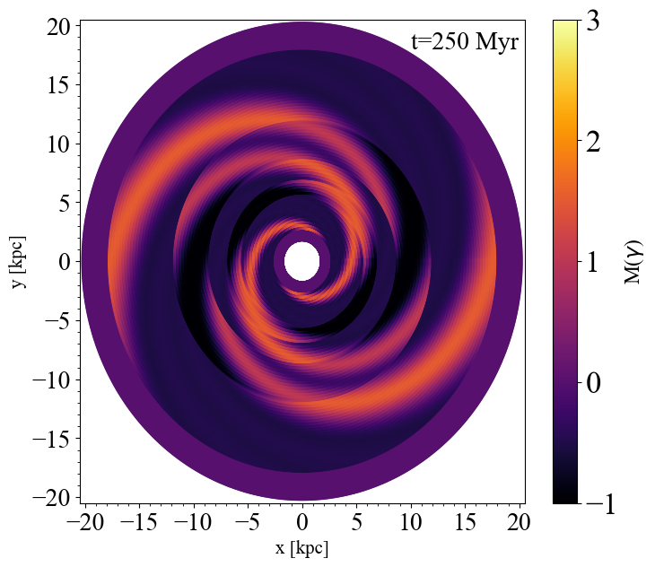
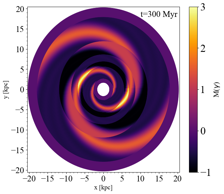
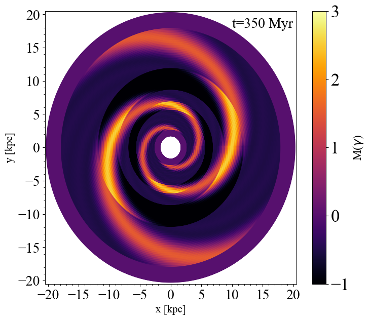
Figure 2: Different snapshots of the temporal evolution of the new modulation function $M(\gamma)\equiv\sum_{j=1}^{3}M_{MS,j}(\gamma_{j})$ introduced in eq. (11) for multiple spiral arm structures assuming the same parameters as Model A reported in Table 1 and also characterised by multiplicity $m=2$ spiral arms, fiducial radius $R_{0}=8$ kpc, pitch angle $\alpha=15^{\circ}$, and $\phi(R_{0})=0.$

Following the same approach as Minchev (2016), in Fig. 1 we show the spiral pattern speeds $\Omega_{s,j}(R)$ of a spiral structure with multiplicity $m=2$ composed by three chunks moving at different pattern speeds $\Omega_{s,j}(R)$ (Model A in Table 1). The $j^{th}$ spiral structures is confined in the region $R\in\left[R_{j,\,\rm min},\ R_{j,\,\rm max}\right]$. As in ES19, the disc rotational velocity $\Omega_{d}(R)$ has been extracted from the simulation by Roca-Fàbrega et al. (2014).

The 2:1 and 4:1 outer and inner Lindblad resonances (OLR and ILR) have been computed as $\Omega_{p2}(R)=\Omega_{d}(R)\pm\kappa/2$ and $\Omega_{p4}(R)=\Omega_{d}(R)\pm\kappa/4$, respectively where $\kappa$ is the local radial epicyclic frequency. The velocity of the central spiral structure is fixed at the value $\Omega_{s,2}$ =20 km s^-1 kpc^-1 that is consistent with the Roca-Fàbrega et al. (2014) model. A similar value was first estimated by moving groups in the U-V plane by Quillen & Minchev (2005, $\Omega$= 18.1$\pm$ 0.8 km s^-1 kpc^-1). It is interesting to note that one of the co-rotational radii is located at 8.75 kpc, hence close to the solar Galactocentric distance $(R,Z)_{\odot}=(8.249,0.0208)$ kpc (GRAVITY Collaboration et al., 2021; Bennett & Bovy, 2019). We stress that recent observations show larger spiral speed values in the solar neighbourhood. For instance, Dias et al. (2019) find a pattern speed of 28.2 km s^-1 kpc^-1 and Quillen et al. (2018) of 29 km s^-1 kpc^-1 at 8 kpc. Nevertheless, to be consistent with the results presented in ES19, we preferred to retain both the velocity disc and the co-rotation estimated in the vicinity of the solar system ($\Omega_{s2}$) by Roca-Fàbrega et al. (2014).

As shown in ES19, the most significant effect of the spiral arms should take place at the co-rotation resonance where the chemical evolution should go much faster due to the lack of the relative gas-spiral motions and more efficient metal mixing. Moreover, it is widely established that discrete spiral waves in stellar disks can exist between their main resonances (ILR-OLR). Since second-order resonances, i.e., 4:1 for a two-armed spiral can also be quite important as shown in Minchev (2016) and giving rise to square orbits in the frame moving with the spiral pattern, in Fig. 1 they have been highlighted.

We stress that also in Castro-Ginard et al. (2021) and Quillen et al. (2018), they find evidence for transient spiral arms, wherein different segments exhibit varying pattern speeds. In this article, we will refer to spiral structures as suggested by Minchev (2016) and Hilmi et al. (2020, see their Section 5.4) with velocity patterns rescaled to the rotational curve of Roca-Fàbrega et al. (2014). Importantly, it should be noted that the methodology introduced in this work possesses versatility and can be expanded to analyse any generic velocity configurations within spiral arms and the disc.

In Fig. 2, we reported different snapshots of the temporal evolution of the modulation function $M(\gamma)\equiv\sum_{j=1}^{3}M_{MS,j}(\gamma_{j})$ introduced in eq. (11) for Model A (see Table 1 for other parameter values). At the initial time, all the spiral chunks trace perfectly a spiral arm structure with multiplicity $m=2$. However, as time goes by, different arc-shaped substructures become more and more prominent in the modulation function map due to the different pattern speeds. It is possible to appreciate that as the number of arcs increases, the amplitude of $M(\gamma)$ decreases. The strength of the perturbation is maximum when we recover the $m=2$ spiral arm configuration after 350 Myr of evolution.

4 Nucleosynthesis prescriptions

As anticipated in the Introduction, the main purpose of this work is to show the results of the azimuthal variations of abundance gradients for oxygen, iron, europium and barium. In this Section, we provide the nucleosynthesis prescriptions for these elements.

4.1 Oxygen and iron

As done in a number of chemical evolution models in the past (e.g. Spitoni et al., 2019b, 2022, 2023; Vincenzo et al., 2019), we adopt for oxygen, iron, the nucleosynthesis prescriptions by François et al. (2004) who selected the best sets of yields required to best fit the data (we refer the reader to their work for the details related to the observational data). In particular, for Type II SNe yields, they found that the Woosley & Weaver (1995) values correspond to the best fit of the data. This occurs because no modifications are required for iron yields, as computed for solar chemical composition, whereas the best results for oxygen are given by yields computed as functions of the metallicity. The theoretical yields by Iwamoto et al. (1999) are adopted for the Type SNeIa, while the prescription for single low-intermediate stellar mass is by van den Hoek & Groenewegen (1997).

Although François et al. (2004) prescriptions still provide reliable yields for several elements, we must be cautious about oxygen. Several results have shown that rotation can affect the oxygen nucleosynthesis in massive stars (Meynet & Maeder, 2002) and, therefore, the chemical evolution (Cescutti & Chiappini, 2010), in particular at low metallicity. However, this does not affect our results since the data shown in this project are relatively metal-rich. Moreover, we are mostly interested in differential effects, rather than absolute values. This set of yields has been widely used in the literature (Cescutti et al., 2007, 2022; Mott et al., 2013; Spitoni et al., 2022, 2023; Palla et al., 2022) and turned out to be able to reproduce the main features of the solar neighbourhood.

4.2 Europium and barium

Neutron star merger (NSM) is considered a fundamental production site for the Eu in our analysis. Following Matteucci et al. (2014) and Cescutti et al. (2015), the realization probability of double neutron star systems belonging to massive stars that will eventually merge, or simply the fraction of such events ($\alpha_{NSM}$).

They adopted a value of 2$\cdot$10^-6 M_⊙ for Eu yields. This is consistent with the range of yields suggested by Korobkin et al. (2012), who propose that NSM can produce from 10^-7 to 10^-5 M_⊙ of Eu per event. Moreover, it was assumed that a fixed fraction of massive stars in the 10-30 M_⊙ range are NSM progenitors. To match the present rate of NSM in the Galaxy (R_NSM=83${}^{+209}_{-66}$ Myr^-1 Kalogera et al. 2004), the parameter $\alpha_{NSM}$ has been set to 0.05. The recent observation of the event GW170817 appears to support this rate (Matteucci, 2021; Molero et al., 2021a).

We set a fixed time delay of 1 Myr for the coalescence of two neutron stars, consistent with the assumptions of Matteucci et al. (2014) and Cescutti et al. (2015). We note that this model assumes all neutron star binaries have the same coalescence time, but a more realistic approach would consider a distribution function of such timescales, similar to the explosion time distribution for SNIa (see Simonetti et al. 2019 and Molero et al. 2021b). In this work, we do not consider the stochasticity of the r-process events. Given the fixed and short delay time considered, the scenario is also compatible with other sources of r-process material such as MRD SNe (Winteler et al., 2012; Nishimura et al., 2015) and collapsar (Siegel et al., 2019). We adopted the yields of Cristallo et al. (2009, 2011) for nucleosynthesis by s-process in low mass AGB stars (1.3 - 3 M${\odot}$), so in this work they play a role in particular for barium. The yields from non-rotating stars were utilised in our analysis, but they tend to overestimate the production of $s$-process elements at solar abundance. In contrast, the yields from rotating AGB stars produce insufficient neutron-capture elements. To address this issue, inspired by Rizzuti et al. (2019) we divide the non-rotating yields by a factor of 2, to reproduce the observed data at solar metallicity. $s$-process contribution from rotating massive stars has also been considered. Initially introduced by Cescutti et al. (2013); Cescutti & Chiappini (2014); Cescutti et al. (2015) using the nucleosynthesis prescriptions proposed by Frischknecht et al. (2012), this study incorporates the yields by Frischknecht et al. (2016), as specified in Table 3 of Rizzuti et al. (2019).

5 Results

In this Section, we present the results of the effect of multiple spiral arm patterns on the chemical evolution of oxygen, iron, europium and barium in the Galactic thin disc. In Section 5.1, we consider the spiral arm pattern speeds as shown in Fig. 1 (Model A in Table 1). In Section 5.2, we will report results for Models A1, A2 and A3 where the 3 spiral structures are considered separately (e.g. arms with single pattern speed) in different runs of the Galactic chemical evolution model (see Table 1 for further details). In Section 5.3 the effects of different angular velocities for the most external spiral structure ($\Omega_{s,3}$) will be discussed (Models B1 and B2).

In Section 5.4, we introduce additional complexities to the spiral arm models presented so far, considering spiral arms with different pattern speeds and modes.

Finally, in Section 5.5 we investigate the hypothesis that, in recent times, all Galactocentric distances are co-rotational radii, which means that the spiral arms are rotating at the same angular velocity as the Galactic disc lately. In fact, several recent numerical studies have shown the possibility of material spiral arms propagating close to the co-rotation at various radii throughout the galaxy (see Grand et al., 2012; Comparetta & Quillen, 2012; Hunt et al., 2019).

All the model results to be presented in this paper adopt the prescriptions from Cox & Gómez (2002) spiral arms analytical model and also applied by ES19: the drop-off in density amplitude of the arms is fixed at a radial scale length of $R_{S}=7$ kpc, the pitch angle is assumed to be constant in time and fixed at the value of $\alpha=15^{\circ}$. The surface arm density, $\Sigma_{0}$, is set to 20 M_⊙ pc^-2 (we refer the reader to ES19 for the motivation of this value) at the fiducial radius of $R_{0}=8$ kpc, and we also assume that $\phi_{p}(R_{0})=0^{\circ}$. It is worth mentioning that, as in ES19 we follow the chemical evolution of the thin disc component, and we assume that the oldest stars are associated with ages of $\sim$11 Gyr, which is in agreement with asteroseismic age estimates (Silva Aguirre et al., 2018).

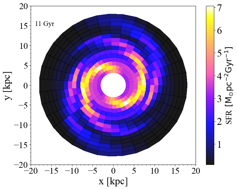
Figure 3: Galactic disc SFR resulting from Model A after 11 Gyr of evolution projected onto the Galactic plane after the start of disc formation (see Table 1 and text for model details). The colour-coding indicates the SFR values in units of M_⊙ pc^-2 Gyr^-1.

Figure 4: A zoom-in view of 2D map of the SFR resulting from Model A after 11 Gyr of the evolution of Fig. 3 compared with some tracers of spiral arms or arcs present in literature. Upper Panel: Overdensities in the distribution of UMS stars of the Poggio et al. (2018) sample with Gaia EDR3 astrometry (Gaia Collaboration et al., 2021) as presented by Poggio et al. (2021). We report only positive values of stellar overdensities as defined by eq. (1) of Poggio et al. (2021). Middle Panel: Distribution of the median of the radial action $J_{R}$ of Gaia DR3 stars (see text for more details) on the Galactic Plane (—$Z_{max}$— ¡ 0.5 kpc and R¡10 kpc) as computed by Palicio et al. (2023a) and here only reporting the star with $J_{R}<0.01$ $R_{\odot}V_{\odot}$ (green shaded area). Lower Panel: Solid lines represent the segments of spiral arms traced by Cepheids of Lemasle et al. (2022) in which the colour coding is the one adopted by Palicio et al. (2023a).

Figure 5: Present-day radial SFR profile predicted by Model A for different azimuthals coordinates (colour lines). In both panels, the shaded light-blue area denotes the range of maximum and minimum SFR values at various Galactocentric distances. Upper Panel: The predicted SFRs are compared with the visible-band observations presented in Guesten & Mezger (1982) and re-scaled by Kennicutt & Evans (2012) to the total SFR of 1.9 M_⊙ yr^-1 of Chomiuk & Povich (2011) as indicated by the black solid line. Lower Panel: Red diamonds with error bars are observational data for the star formation profile from SN remnants, pulsars, and HII regions normalised to the solar vicinity value (SFR/SFR_⊙) from Stahler & Palla (2004). The dark-blue solid represents the analytical fit of SN remnants compilation by Green (2014) as reported in Palla et al. (2020) and Spitoni et al. (2021). The model predictions for different azimuths SFR_ϕ are divided by their respective solar vicinity SFR_⊙,ϕ values.

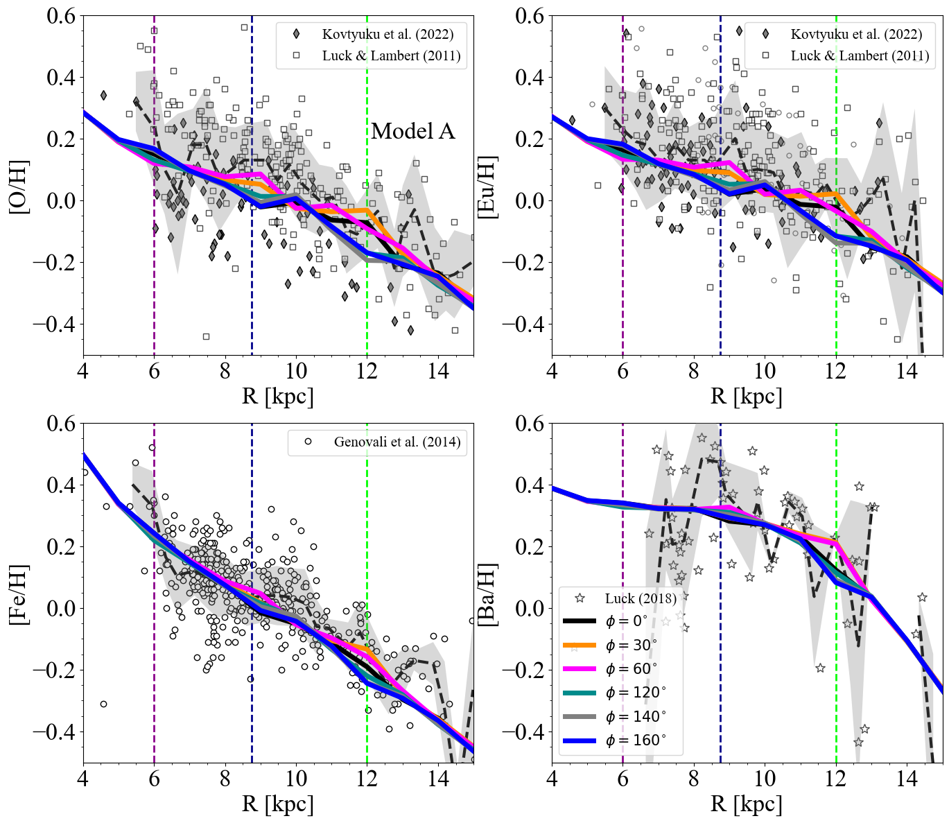
Figure 6: Present-day oxygen (upper left panel), europium (upper right panel), iron (lower left panel) and barium (lower right panel) abundance gradients for different azimuths as predicted by the Model A (see Table 1 for model details). In each panel, the coloured dashed vertical lines indicate the location of the co-rotation radii for the three spiral structures characterised by different pattern speeds. Model predictions are compared with Cepheids data by Kovtyukh et al. (2022) and Luck & Lambert (2011) for oxygen and europium, by Genovali et al. (2014) for iron and by Luck (2018) for barium. The data trends (black dashed lines) are computed by calculating the running median in bins of 0.5 kpc, with a 40% overlap, and a minimum number of stars per bin of two for O, Fe and Eu, and one for Ba due to the low number of measurements in the sample. The shaded regions on the plot represent the standard deviation of these trends. For the sake of visualisation, we focus on the abundance range [-0.5, 0.6] dex, excluding stars with [Ba/H]¿0.6 dex.

5.1 Multi-pattern spiral arm structure: Model A

In Fig. 3, the predicted 2D map of the SFR projected onto the Galactic disc by Model A after 11 Gyr of Galactic disc evolution (present-day) is shown. Although the considered spiral arms have multiplicity $m=2$, the signatures of multiple arcs and substructures originated by different velocity patterns are well visible in the regions with enhanced star formation. In the upper panel of Fig. 4, the position of the spiral arms in the Galaxy as mapped by the overdensities of upper main sequence (UMS) stars of Poggio et al. (2021) is overplotted on the predicted presented day SFR by Model A (the same as Fig. 3). In this plot, we report the stellar overdensities as defined by eq. (1) of Poggio et al. (2021) for positive density contrast values.

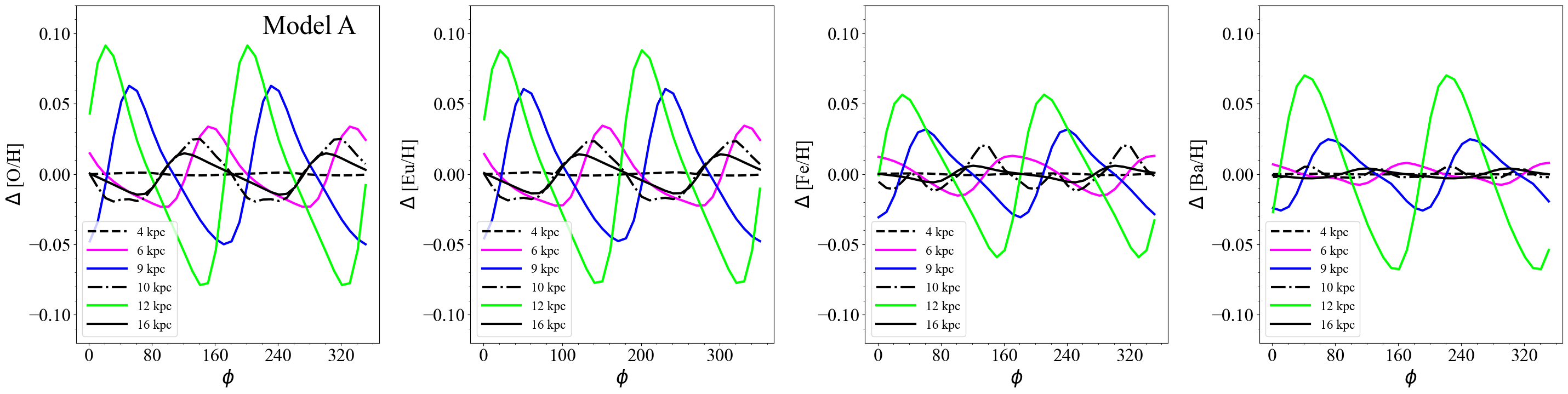
Figure 7: Present-day residual azimuthal variations in oxygen, europium, iron and barium abundance, respectively computed at different Galactocentric distances for the multiple spiral structure of Model A in Table 1. The coloured solid lines indicate the variations at the co-rotation radii for the three spiral structures characterised by different pattern speeds with the same colour-coding as the dashed vertical lines of Fig. 6.

In the middle panel, we show the map of the median of the radial action $J_{R}$ on the Galactic Plane (—$Z_{max}$— ¡ 0.5 kpc and R¡10 kpc) as computed by Palicio et al. (2023a) for Gaia DR3 stars with full kinematic information only for bins with $J_{R}<0.01$ $R_{\odot}V_{\odot}$, which trace the innermost region for the Scutum-Sagittarius spiral arms. For stars in the disc, $J_{R}$ can be interpreted as a parameter that quantifies the oscillation in the radial direction, with $J_{R}=0$ for circular orbits. We refer the reader to Appendix B of Palicio et al. (2023a) for a detailed explanation of how the radial action $J_{R}$ has been computed.

Finally, in the lower panel, the solid lines represent the segments of spiral arms traced by Cepheids in Lemasle et al. (2022). We note that there is good agreement between the above-mentioned spiral arms tracers and the location of the predicted enhanced star formation regions driven by the passage of the multiple pattern spiral arm of Model A. In Fig 5, we note that the present-day SFR profiles predicted by Model A at different azimuthal coordinates throughout the Galactic disc are in agreement with the visible-band observations presented by  Kennicutt & Evans (2012), Stahler & Palla (2004, SN remnants, pulsars, and HII regions), and Green (2014, SN remnants).

In Fig. 6, we report for O, Eu, Fe and Ba the present-day abundance gradients predicted by Model A after 11 Gyr of evolution for different azimuthal coordinates. It is important to stress that, as already found by Cescutti et al. (2007) and more recently by Molero et al. (2023), the predicted gradient for barium is almost flat or slightly decreasing in the innermost Galactic regions.

As already underlined in the analysis of the azimuthal variation of oxygen in ES19, the more significant variations are located close to the co-rotation. We note that as the co-rotation is shifted towards the outer Galactic regions, variations become more enhanced. This is in agreement with the results of ES19, where the density perturbation extracted by the chemo-dynamical model of Minchev et al. (2013) was included. In fact, also in this case significant variations have been found in chemical abundances in the outer Galactic regions.

Spitoni et al. (2019a) stressed that the chemical enrichment process at the co-rotation is expected to be more efficient because of the absence of relative gas-spiral motions. The co-rotation radius experiences a higher star formation rate (SFR) due to increased gas overdensity, which persists for a longer duration. This leads to the formation of more massive stars and the ejection of more metals into the local interstellar medium (ISM). To illustrate this, we represent in Fig. 7 the excess of chemical abundances with respect to the azimuthal average.

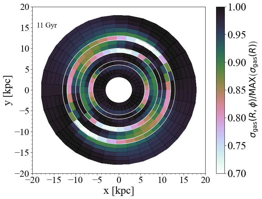
Figure 8: Galactic disc surface gas density distribution resulting from Model A after 11 Gyr of evolution normalised to the maximum values at different Galactocentric distances. We also highlight with white edges the annular regions where three co-rotational radii are situated.

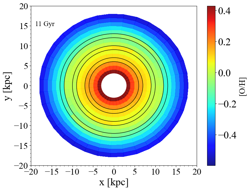
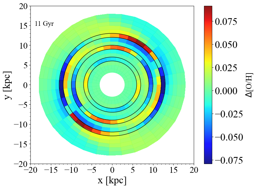
Figure 9: Galactic disc oxygen abundances distribution resulting from Model A after 11 Gyr of evolution projected onto the Galactic plane after the start of disc formation (see Table 1 and text for model details). Upper panel: [O/H] values are reported. Lower panel: The distribution of residual azimuthal variations $\Delta$ [O/H] in oxygen are drawn. In each panel, we also highlight with black edges the annular regions where the three co-rotational radii are situated.

With this model, we can make predictions on the azimuthal variations originating from spiral arm structures for different chemical elements. From Fig. 6, it is clear that azimuthal variations depend on the studied chemical element: elements produced on short time-scales (i.e., oxygen almost totally synthesised in Type II SNe and europium in NSM and via $r$-processes) show the largest variations. Since the progenitors in these cases have short lifetimes, the chemical elements restored into the ISM trace perfectly the SFR fluctuations created by the spiral arm mass overdensities. It results in a pronounced variation in the abundance gradients compared with other elements ejected into the ISM after an important time delay. For example, the bulk of iron is produced by Type Ia SNe and the timescale for restoring it into the ISM depends on the assumed supernova progenitor model and the associate delay time distribution (Greggio, 2005; Matteucci et al., 2009; Palicio et al., 2023b). The typical timescale for the Fe enrichment in the Milky Way solar neighbourhood is around 1-1.5 Gyr (Matteucci et al., 2009). From Fig. 6, we note that a larger spread in the chemical abundances is present also in the Cepheid data for elements produced in short time-scales (oxygen and europium) compared to iron, in agreement with our model predictions. For the barium, too few stellar abundances are available to make any firm consideration.

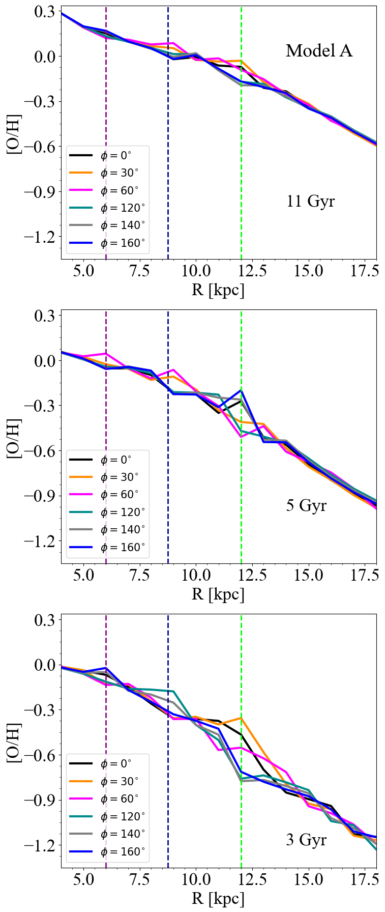
Figure 10: Temporal evolution of the oxygen abundance gradient after 3, 5, and 11 Gyr of thin disc evolution for different azimuth coordinates as predicted by Model A. Color code is the same as in Fig 6.

In our approach we neglect dynamical processes that could affect the gas distribution in the co-rotations. For instance, Barros et al. (2021) pointed out, from both hydrodynamic analytical solutions and simulations, that the interaction of the gaseous matter of the disk with the spiral perturbation should produce a flow of gas that establishes at the co-rotation region. In particular, an inward flow of gas to the inner regions of the Galaxy and an outward flow to the outer regions are present at the co-rotation circle, from which the flows diverge. As a natural consequence of this dynamic process, a ring-shaped void of gas should form at the co-rotation radius. Nonetheless, Lépine et al. (2017) showed that the Local Arm is an outcome of the spiral co-rotation resonance, which traps arm tracers and the Sun inside it. Hence, it supports the scenario where some mass should cluster inside the co-rotation zones, thereby contributing to increased density in these regions. In conclusion, two processes with opposite effects (gas depletion and clustering) seem to coexist, and it is still not clear which is the dominant one.

In our model, the lack of relative velocity between disc and spiral structures is the main cause of the pronounced azimuthal abundance variation at the co-rotation. As shown in Fig. 8, we have significant dips in gas distribution at the three co-rotational radii. However, these declines align exclusively with positive variations in chemical abundance (see Fig. 9). In light of the dynamical results mentioned by Barros et al. (2021), our findings must be considered as an upper limit of the azimuthal variations originated by spiral arms. On the other hand, it is important to point out that in the chemodynamical simulations of the Milky Way-like spiral galaxies as presented by Khoperskov et al. (2023), there is no evidence of any annular void region in the gas distribution (see their Figure 2), which is a signature of the presence of co-rotation, as suggested Barros et al. (2021).

Scarano & Lépine (2013), analysing external galaxies, claimed that the presence of a step in metallicity and the change of slope of the gradient at this radius is due to the co-rotation. However, it is important to underline that a change in the slope in the abundance gradient can be the result of other chemo-dynamical processes such as the inside-out formation scenario, variable star formation efficiency or IMF throughout the Galactic disc (see Matteucci 2021 for a review).

In Fig. 10, we show the temporal evolution of the oxygen abundance gradients after 3, 5, 9 and 11 Gyr of evolution. At early times, the azimuthal variations are more prominent as already pointed out by ES19.

As the oxygen abundance increases (i.e. closer to the ”saturation” level of the chemical enrichment), the smaller the chemical variations due to perturbations of the SFR are observed. In addition, the Galactic chemical evolution is a cumulative process in time. In early times, the stronger spiral structure induced azimuthal variations, which are later washed out by phase mixing. Hence, we provide an important prediction for the high redshift galaxies with spiral arms that will be analysed in future works, especially thanks to James Webb Space Telescope (JWST) discoveries. In fact, Fudamoto et al. (2022), analysing the initial image captured by JWST of SMACS J0723.3-7327, highlighted the presence of two extremely red spiral galaxies likely in the cosmic noon (1 ¡ $z$ ¡ 3).

Table 2: Maximum azimuthal residual variations $\Delta_{\rm max}$ [X/H] for oxygen, europium, iron and barium predicted by models B1 and B2 at the respective co-rotations of the outermost spiral chunk (characterised by angular velocity $\Omega_{s,3}$ and the co-rotation radius $R_{3,{\rm cor.}}$).

Models	$\Omega_{s,3}$	$R_{3,{\rm cor.}}$	$\Delta{\rm max}$ [O/H]3,cor.	$\Delta{\rm max}$ [Eu/H]3,cor.	$\Delta{\rm max}$ [Fe/H]3,cor.	$\Delta{\rm max}$ [Ba/H]3,cor.
	[km s-1 kpc-1]	[kpc]	[dex]	[dex]	[dex]	[dex]
B1	17.00	10.25	0.134	0.127	0.075	0.069
B2	13.00	13.30	0.186	0.177	0.120	0.156

5.2 Single-pattern spiral arms (Models A1, A2, and A3)

Recent investigations pointed out that it is very likely that the Milky Way possesses multiple modes with different patterns, with slower patterns situated towards outer radii (Minchev & Quillen, 2006; Quillen et al., 2011). In ES19, only the effects of spiral arms with single patterns in a chemical evolution model (e.g., considering diverse velocities solely in different Galactic models) were presented. In order to be in agreement with the observations of external galaxies (Sánchez et al., 2015), and with the results obtained using as fluctuations the ones form the chemodynamical model of Minchev et al. (2013), the authors assumed that the modes with different patterns combine linearly, and their total effects on abundance azimuthal variations respond linearly to different modes considered. We confirmed this hypothesis by testing that the sum of residual azimuthal variations predicted for Models A1, A2 and A3 (i.e. models where the 3 chunks of spiral arms are considered separately, see Table 1) is almost identical to the ones of Model A:

$$\Delta\text{[O/H]}_{\text{A}}\simeq\Delta\text{[O/H]}_{\text{A1}}+\Delta\text{[O/H]}_{\text{A2}}+\Delta\text{[O/H]}_{\text{A3}}.$$ (14)

We conclude that in our approach we do not find any amplifications of the azimuthal variation in the zones where the different chunks of spiral arms are connected and spatially overlap.

5.3 Varying the pattern velocity for the external spiral structure: Models B1 and B2

Models B1 and B2 (see Table 1), have the same pattern speed $\Omega_{s,1}$ and $\Omega_{s,2}$ and radial extension of the two innermost spiral structures as Model A, but for the external clump diverse velocities have been tested to quantify the effects of different external co-rotational radii. In Model B1, the velocity of the outermost spiral chunk is $\Omega_{s,3}=$ 17 km s^-1 kpc^-1 (i.e. the co-rotation is located at 10.25 kpc from the Galactic centre). On the other hand, in Model B2 we impose that $\Omega_{s,3}=$ 13 km s^-1 kpc^-1 (i.e. a co-rotation located at 13.30 kpc).

In Table 2, we reported the maximum residual azimuthal variations $\Delta_{\rm max}$ [X/H] for oxygen, europium, iron and barium predicted by models B1 and B2 at the respective co-rotations of the outermost spiral chunk characterised by angular velocity $\Omega_{s,3}$. We confirmed that the lower the velocity $\Omega_{s,3}$ is, and the most prominent amplitudes of the azimuthal variations are, as already discussed in previous Sections and in ES19. It is evident that a difference in the pattern speed of $\Delta\Omega_{s,3}=4$ km s^-1 kpc^-1 in the most external spiral mode leads to a shift of the co-rotation radius of roughly 3 kpc and has substantial effects on the chemical evolution of the Galactic disc.

5.4 Spiral arms with different pattern speeds and modes

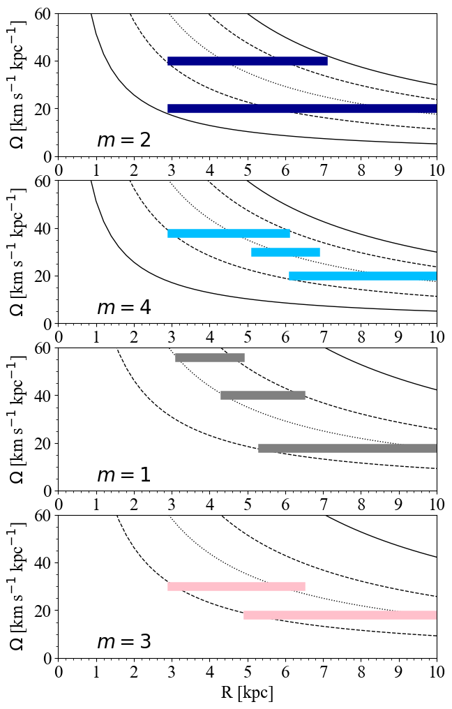
Figure 11: As Fig. 1, but for spiral modes extracted from the spectrogram analysis of Model1 by Hilmi et al. (2020), based on the Buck et al. (2020) cosmological simulation. Different multiplicities are shown in each panel, as indicated. In each panel, the disc angular velocity $\Omega_{d}(R)$ is indicated with the dotted line. In the two upper panels (with modes $m=2$ and $m=4$), we also show the resonances $\Omega_{p2}(R)=\Omega_{d}(R)\pm\kappa/2$ and $\Omega_{p4}(R)=\Omega_{d}(R)\pm\kappa/4$, indicated with solid and dashed black curves, respectively. In the last two panels solid and dashed black have been computed as $\Omega_{p1}(R)=\Omega_{d}(R)\pm\kappa$ and $\Omega_{p3}(R)=\Omega_{d}(R)\pm\kappa/3$.

In this Section, we introduce additional complexities to the spiral arm models presented so far, with the aim of examining the influence of multiple patterns and different modes on the chemical evolution of the thin disc. We extracted the pattern speeds from the power spectrogram constructed by Hilmi et al. (2020) of the $m$ = 1, 2, 3, and 4 Fourier components using a time window of 350 Myr for their Model 1. This model is based on the high-resolution hydrodynamical simulations of MW-sized galaxies from the NIHAO-UHD project of Buck et al. (2020) (galaxy g2.79e12).

In Fig. 11, we present the velocity patterns for various modes extracted by Hilmi et al. (2020) and scaled to the circular velocity determined by Roca-Fàbrega et al. (2014). In analogy with eq. (10), the expression for the time-evolution of the density perturbation created by different speeds and modes of Fig. 11 can be written as:

$$\Sigma_{MS}(R,\phi,t)=\chi(R,t_{G})\sum_{m=1}^{4}\left(A_{m}\sum_{j=1}^{N_{m}}M_{MS_{m},j}\,(\gamma_{j})\right),$$ (15)

where $N_{m}$ is the number of spiral clumps associated with the mode $m$. The coefficients $A_{m}$ are set by adopting the power spectrograms from figure 11 of Hilmi et al. (2020) to redistribute the spiral density perturbation across different modes ($A_{1}$=0.1, $A_{2}$=0.4, $A_{3}$=0.1 and $A_{4}$=0.4). In Fig. 12, we display the residual azimuthal variations in oxygen, europium, iron, and barium abundance at the present day, calculated at distances of 4, 6, and 9 kpc.

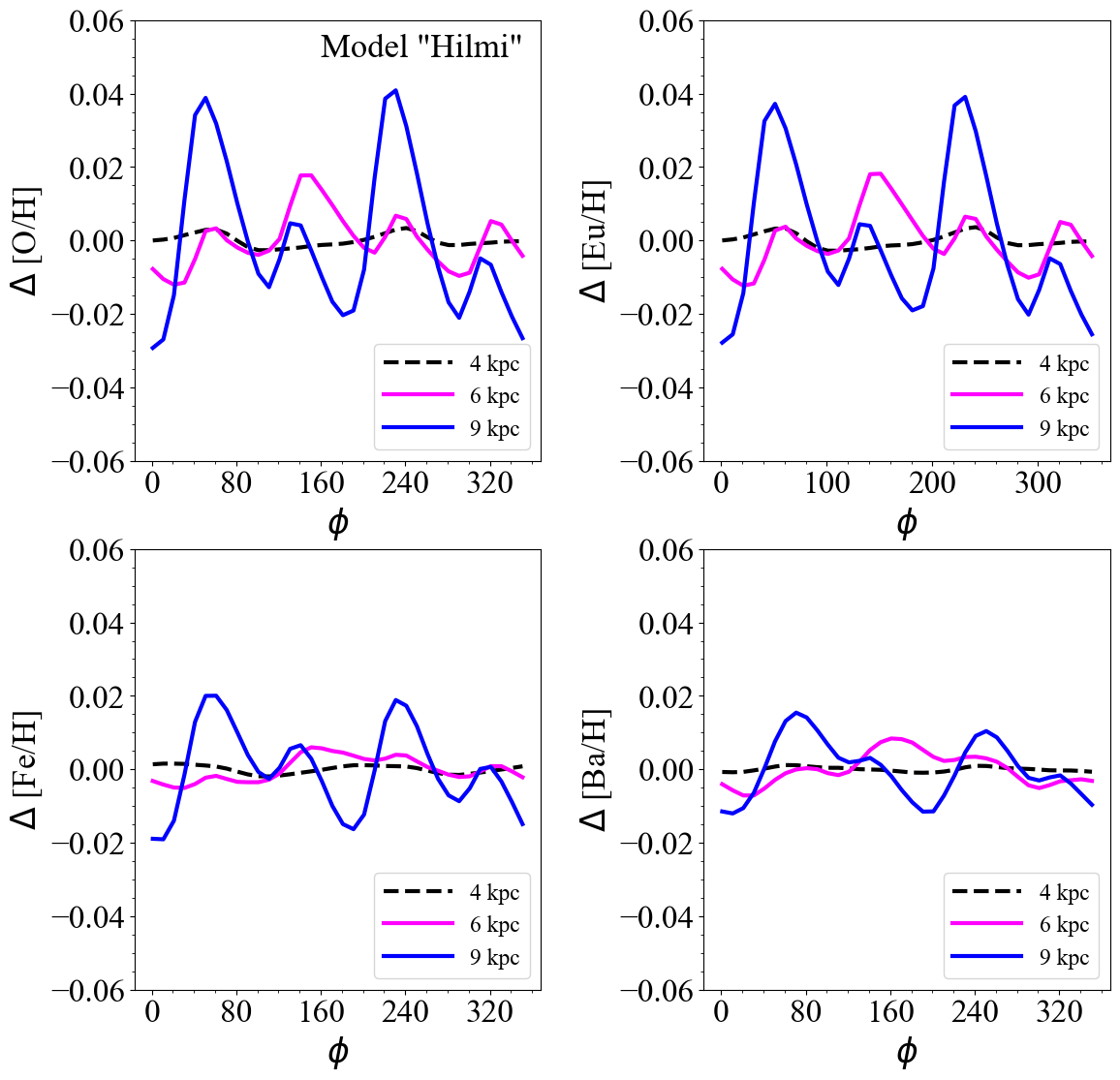
Figure 12: Present-day residual azimuthal variations in oxygen, europium, iron and barium abundance, respectively computed at 4, 6 and 9 kpc for Model1 by Hilmi et al. (2020), as introduced in Section 5.4, where the spiral structure is characterised multiple modes of different multiplicity from 1 to 4.

It is worth underlining the presence of additional wiggles in the azimuthal variations compared to the results of Model A (see Fig. 7, where the single mode $m=2$ was imposed), which arise from the coexistence and interplay of different modes. However, the amplitude of the azimuthal variation at 9 kpc remains roughly the same. Therefore, in the subsequent section, we will employ Model A as our reference model for further investigations.

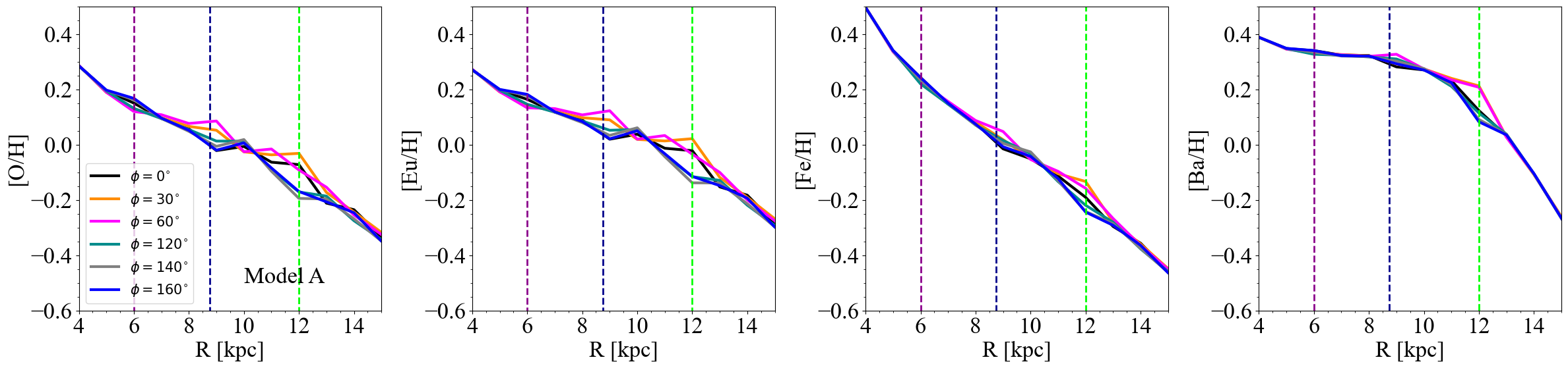
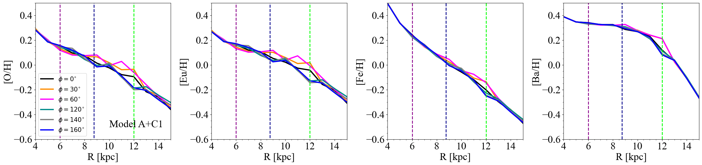
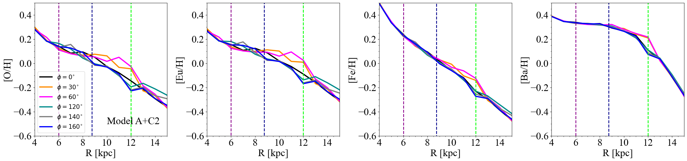
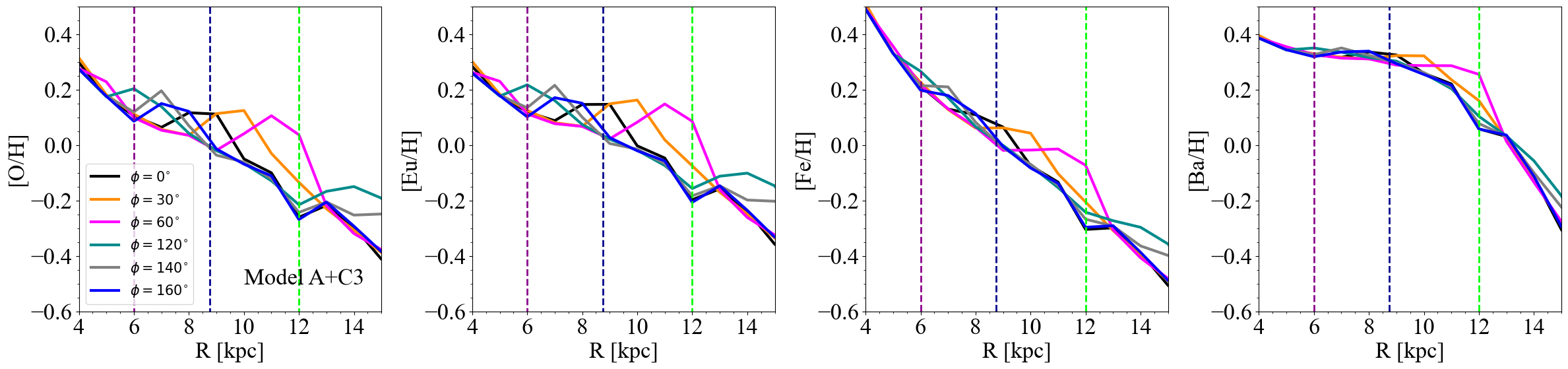
Figure 13: Comparing azimuthal variations in abundance gradients for oxygen, europium, iron and barium predicted by Model A (first row) with models where the condition of transient spiral have been considered. Model A+C1 where in the last 100 Myr of Galactic evolution the condition $\Omega_{s,j}(R)=\Omega_{d}(R)$ is valid for all the Galactic radii (co-rotation extended at all distances) is reported in the second row, Model A+C2 when the above-mentioned condition lasted for the last 300 Myr in the third row, Model A+C3 for 1 Gyr in the last row. Colour convention of the lines as in Fig. 6. The vertical lines indicate the corotations of Model A.

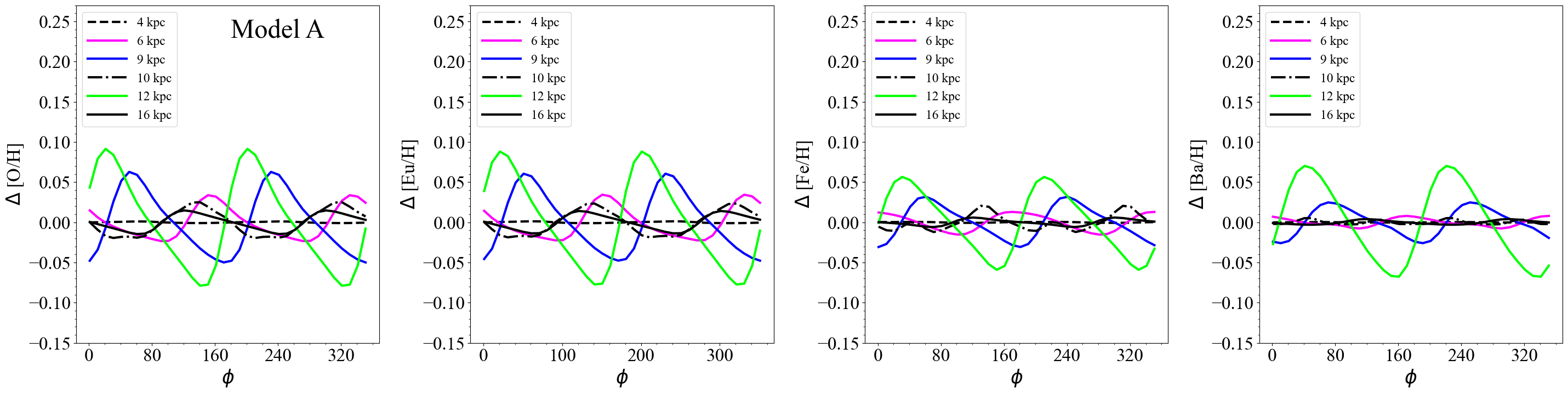
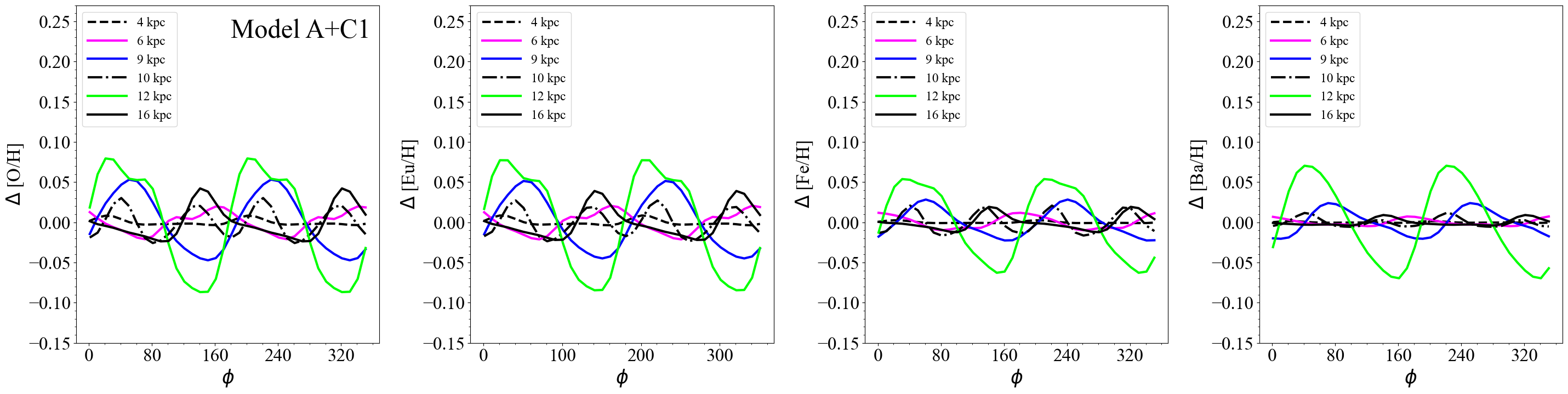
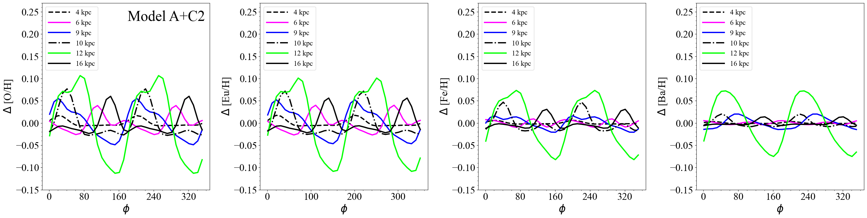
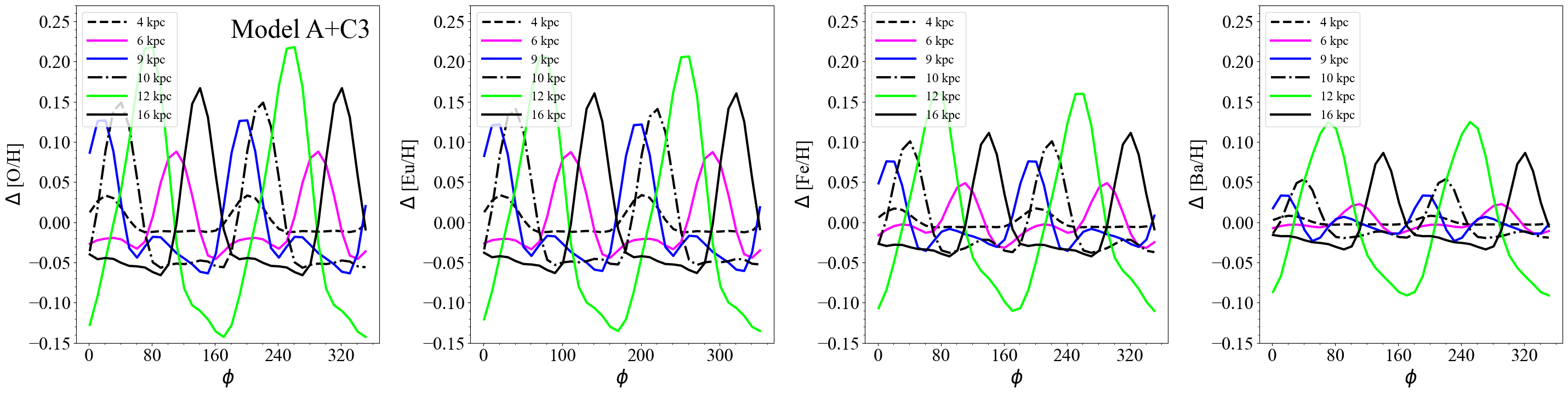
Figure 14: As in Fig. 7, but also for Model A+C1 (second row), Model A+C2 (third row) and Model A+C3 (last row), respectively.

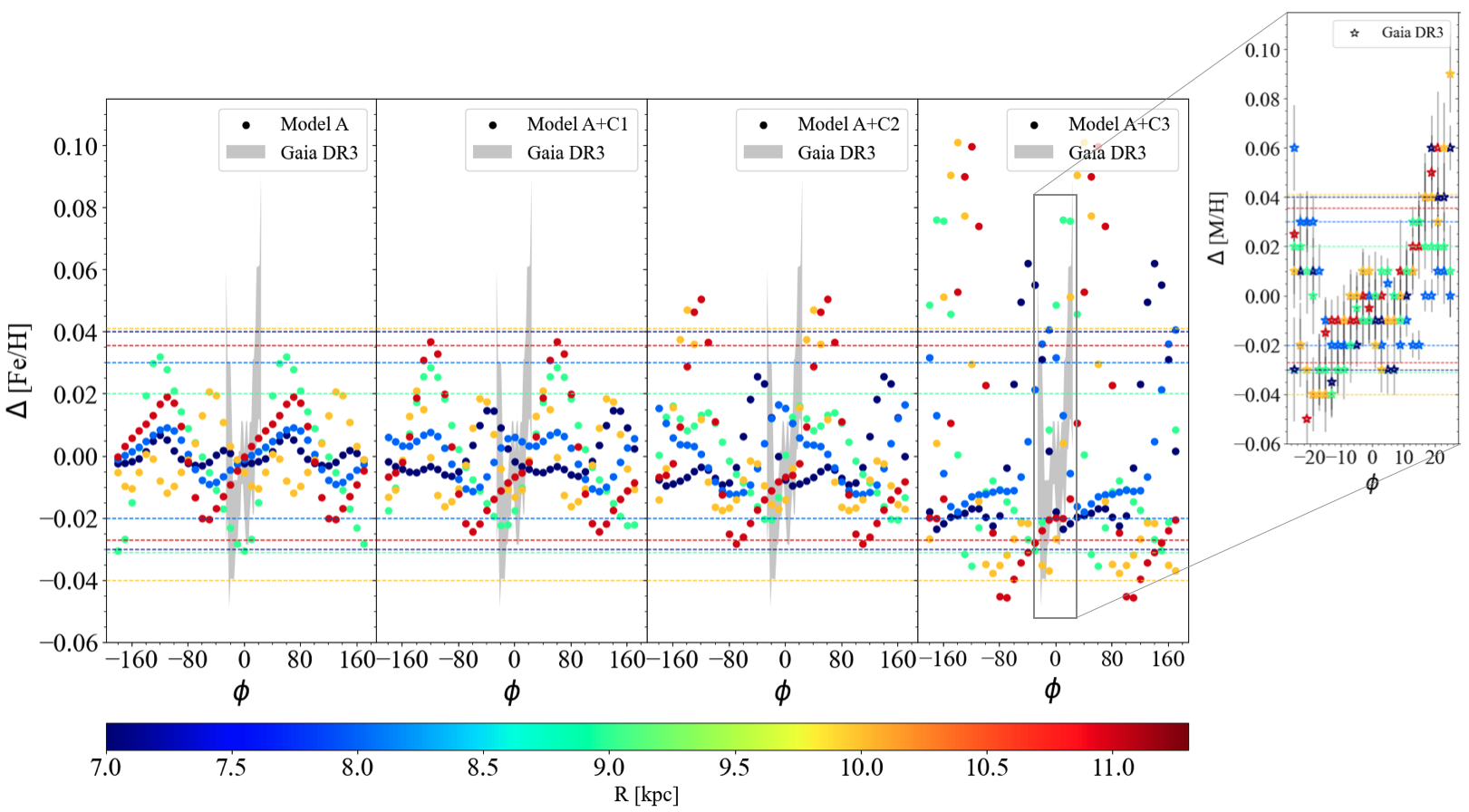
Figure 15: Present-day residual azimuthal variations in iron respectively computed at different Galactocentric distances for the multiple spiral structure of the Model A, A+C1, A+C1 and A+C3, compared with metallicity variation found by Poggio et al. (2022) analysing GSP-Spec abundances of Gaia DR3 Gaia Collaboration et al. (2023) (grey shaded regions). Horizontal lines with the same colour indicate the 10$\%$ and 90 $\%$ percentiles of the metallicity variation as computed by Poggio et al. (2022) at different Galactocentric distances. In each panel, the shaded grey area indicates the region spanned by Poggio et al. (2022) data. In the zoom-in plot associated with the fourth panel, we report the Poggio et al. (2022) data indicating median metallicity for Sample A as a function of Galactic azimuth for different Galactocentric distances (after the median metallicity of the stars for each ring has been subtracted).

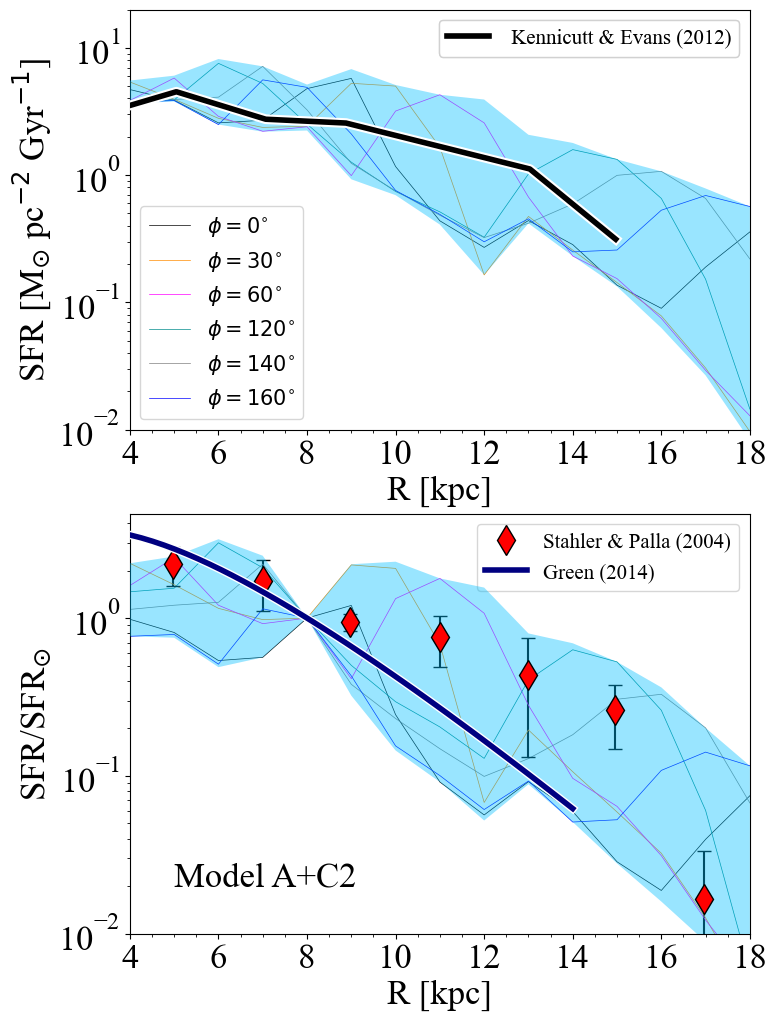
Figure 16: As in Fig. 5 but for the Model A+C2.

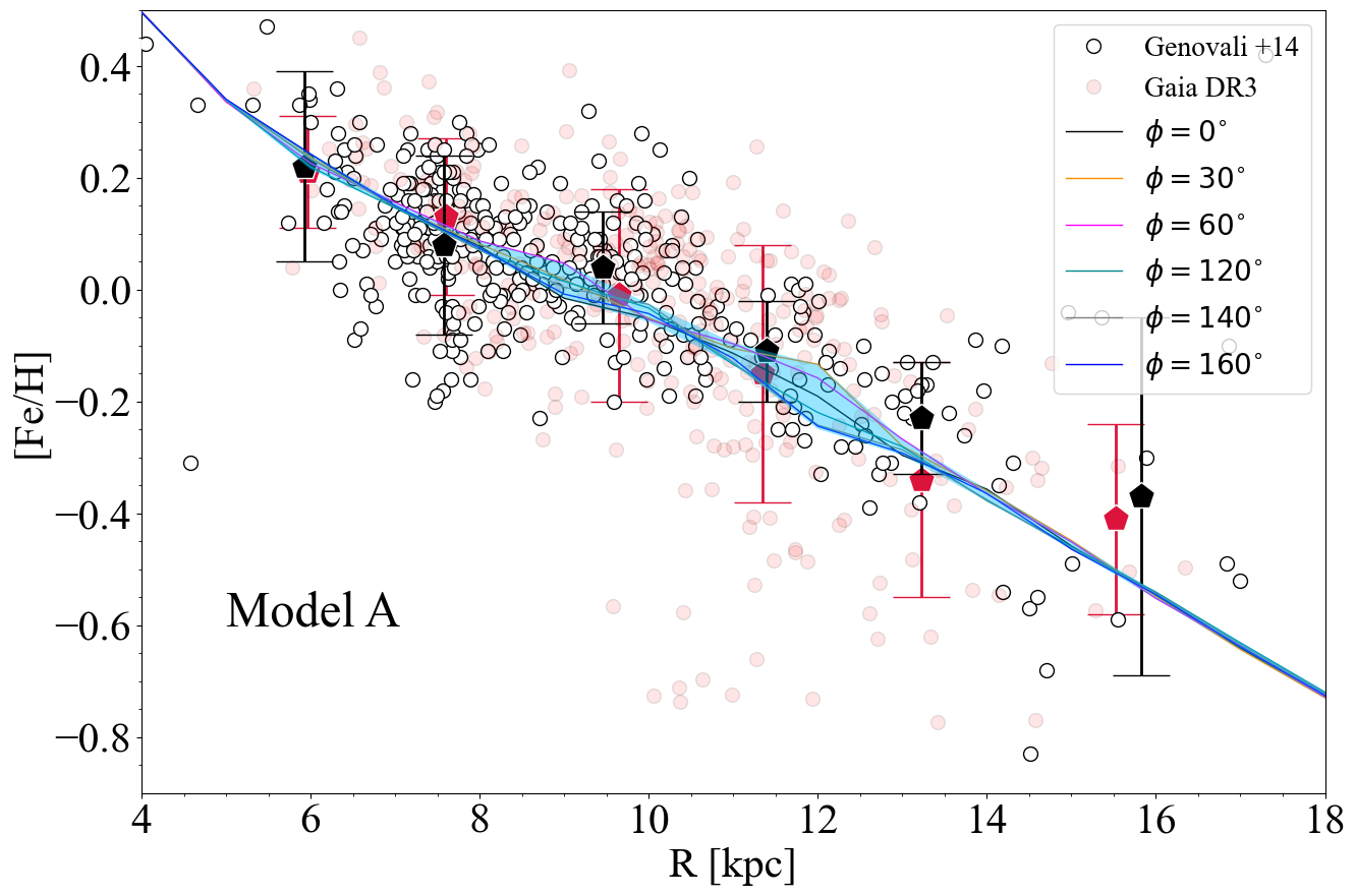
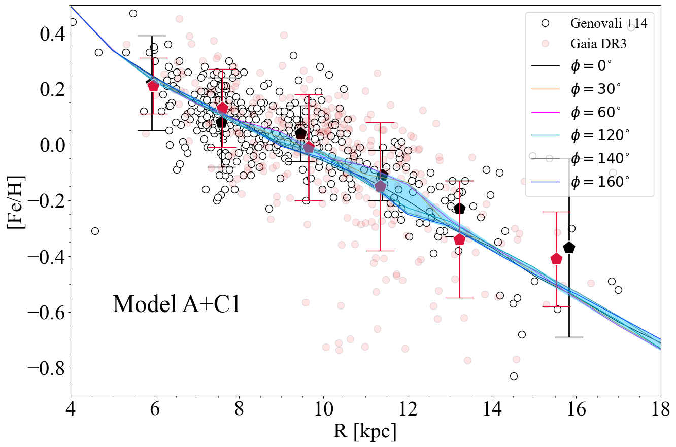
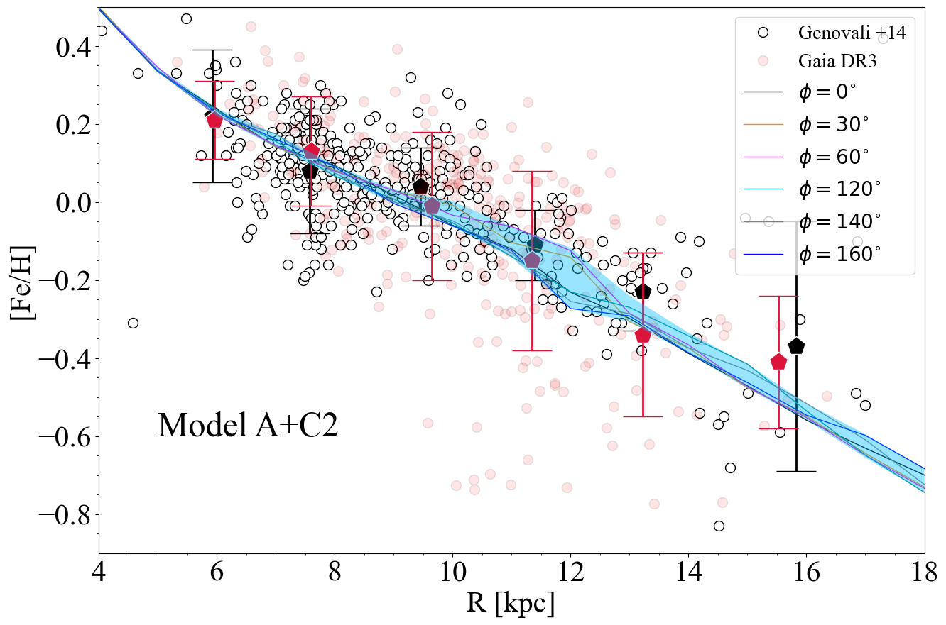
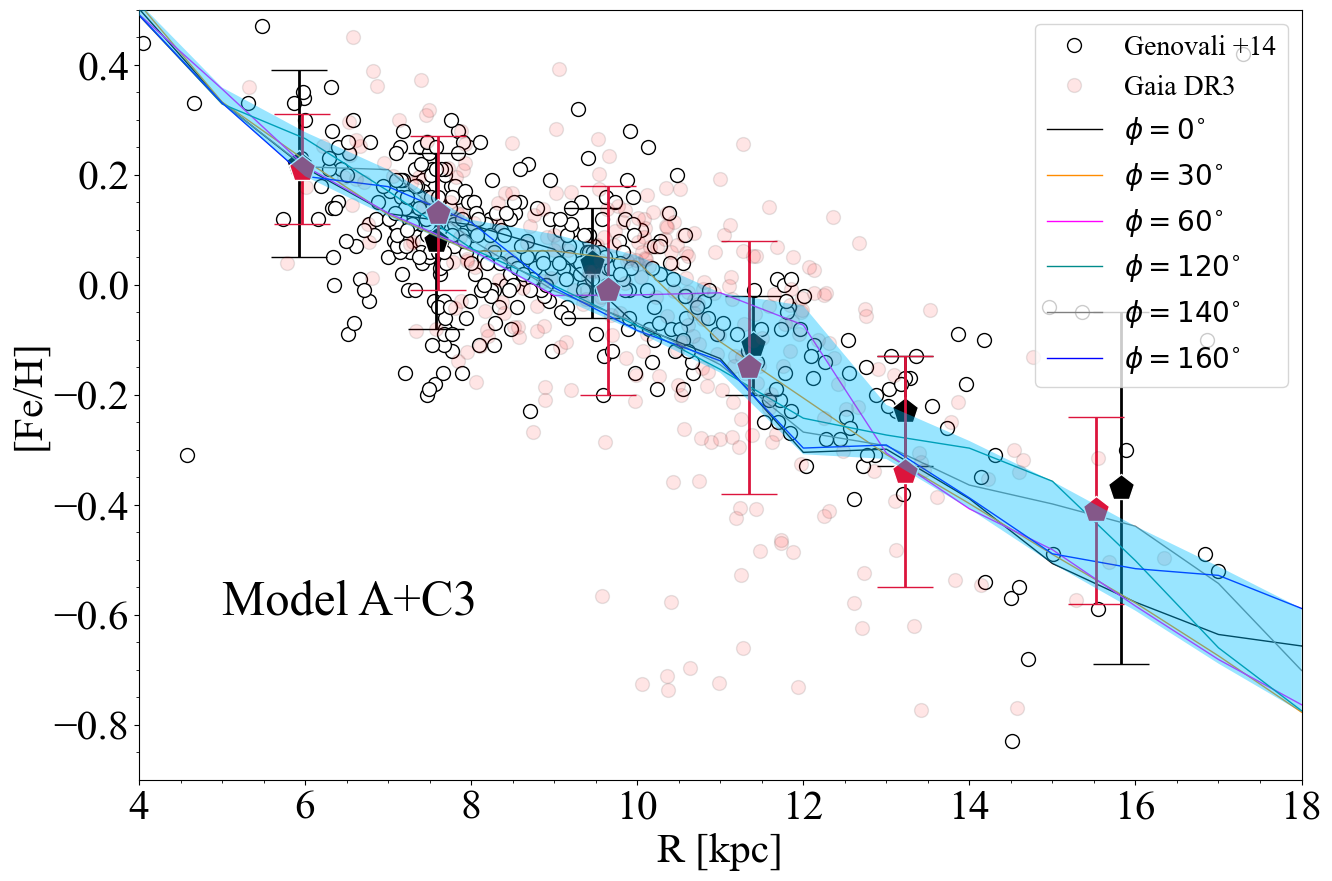
Figure 17: Present-day iron abundance gradient predicted by Models A, A+C1, A+C2 and A+C3 at different azimuthal coordinates. In each panel, the shaded light-blue area denotes the range of maximum and minimum Fe abundance values at various distances from the centre of the galaxy spanned by the models. The Cepheids data collected by Genovali et al. (2014) and GSP-Spec [M/H] for Gaia DR3 source id of Cepheids of Ripepi et al. (2023) are reported with empty and full light-red dots, respectively. The average abundance values and relative errors, when dividing these two data sets into six radial bins, are shown by black and red pentagons, respectively.

5.5 Extending the co-rotation to all Galactocentric distances (Models A+C1, A+C2, A+C3)

The results of chemical evolution models presented so far are based on the evidence that the Milky Way can contain multiple patterns, with slower patterns situated towards outer radii (Minchev & Quillen, 2006; Quillen et al., 2011). Furthermore, in other dynamical works (Grand et al., 2012; Hunt et al., 2019) co-rotating arms can be found at all radii in transient spiral arm structures.

The occurrence of temporary spiral structure results in phase mixing, leading to the formation of ridges and arches in the nearby kinematics observed in the Gaia data (Gaia Collaboration et al., 2023; Gaia Collaboration, Antoja et al., 2021; Ramos et al., 2018; Palicio et al., 2023a). By incorporating a bar with various pattern speeds, Grand et al. (2012); Hunt et al. (2019) successfully generated a reasonably accurate resemblance to the observations. In addition, in the pure N-body simulation of Grand et al. (2012) of a barred galaxy, the spiral arms are transient features whose pattern speeds decline with the radius, so that the pattern speed closely matches the rotation of star particles.

To mimic the above-mentioned scenarios, we impose that at recent evolutionary times, the pattern speeds $\Omega_{s,j}$ match the rotational curve at all radii, i.e the condition $\Omega_{s,j}(R)=\Omega_{d}(R)$ is extended to all Galactocentric distances for each of the spiral chunks of Model A. As indicated in Table 1, we applied this condition for the last 100 Myr of Galactic chemical evolution (Model A+C1), 300 Myr of evolution (Model A+C2) and 1 Gyr (Model A+C3), respectively.

In Figs. 13 and 14, we presented the abundance gradients and the residual azimuthal variations predicted by these three new models. As expected, the amplitudes for the considered chemical elements are amplified compared with Model A, especially at Galactocentric distances different from that of the corotations of Model A, as visible in Figs. 13 for Models A+C1 and A+C2. The longer the condition for the transient spiral arm, the larger the amplitude of the azimuthal variation. In fact, as discussed in previous Sections, the condition $\Omega_{s,j}(R)=\Omega_{d}(R)$ imposes that, at fixed Galactocentric distance $R$ and azimuthal coordinate $\phi$, the perturbation term $\delta_{MS}$ (introduced in eq. 12) in the SFR does not vary in time. Hence, the chemical fluctuation should be amplified. The extreme case of Model A+C3 with the condition $\Omega_{s,j}(R)=\Omega_{d}(R)$ in the last 1 Gyr, should be considered as a test (see last rows in Figs. 13 and 14). For instance, for oxygen, the maximum amplitude at 12 kpc is $\Delta_{max}$[O/H]$\sim$ 0.37 dex, whereas for Model A was $\Delta_{max}$[O/H]$\sim$ 0.17 dex, hence increased by a factor of 2.18.

5.5.1 Tightly wound spiral structures

The work of Quillen et al. (2018) and Laporte et al. (2019) suggested that tightly wound spiral structures should be considered based on the modelling of phase-space structure found in the second Gaia data release (Gaia Collaboration et al., 2018). A smaller pitch angle gives rise to a more tightly wound spiral structure. In Reshetnikov et al. (2023), they study pitch angles of spiral arms in galaxies within the Hubble Space Telescope COSMOS field. Analysing a sample of 102 face-on galaxies with a two-armed pattern they found a decreasing trend in the pitch angle value from a redshift range of $z=1$ to $z=0$. However, in this study, we do not test the effects of a decreasing pitch angle in time on the chemical evolution of the Galactic disc. In fact, as already pointed out by ES19, the amplitude of the azimuthal variation in the abundance gradients is not dependent on the pitch angle. As highlighted by Fig. 18 of ES19, small pitch angles solely reduce the phase difference of the abundance variation between different radii.

6 Gaia DR3 data

Gaia DR3 (Gaia Collaboration, Vallenari et al., 2022) and Recio-Blanco et al. (2023); Gaia Collaboration et al. (2023) have brought a truly and unprecedented revolution opening a new era of all-sky spectroscopy. With about 5.6 million stars, the Gaia DR3 General Stellar Parametrizer - spectroscopy (GSP-Spec, Recio-Blanco et al. 2023) all-sky catalogue is the largest compilation of stellar chemo-physical parameters and the first one from space data without the issues of biased samples which hampered the observations from Earth. In Gaia Collaboration et al. (2023), the high quality of the GSP-Spec chemical abundances for $\alpha$-elements and Fe have been used to provide important constraints on the Galactic Archaeology. Updated chemical evolution models for the evolution of the thick and thin discs have been presented by Spitoni et al. (2023) constrained by $\alpha$-elements in the solar vicinity. The interaction with the Sagittarius dwarf galaxy could explain the observed feature in the abundance ratios. In Contursi et al. (2023), they analysed the GSP-Spec cerium unveiling the evolution history of this heavy element.

In Section 6.1 we compare our model predictions with the azimuthal variations found in the metallicity distribution of Poggio et al. (2022), whereas in Section 6.2 we compare them with the GSP-Spec [M/H] abundance ratios of Cepheids.

6.1 Comparison with Poggio et al. (2022)

Poggio et al. (2022) exploited Gaia DR3 data providing a map of inhomogeneities in the Milky Way’s disc [M/H] abundances, which extends to approximately 4 kpc from the solar position. This was achieved by studying various samples of bright giant stars, which were selected based on their effective temperatures and surface gravities using the GSP-Spec module. Their Sample A, composed of hotter (and younger) stars, exhibits significant inhomogeneities, which manifest as three (possibly four) metal-rich elongated features that correspond to the spiral arms’ positions in the Galactic disc. In Fig. 15, we compare the present-day residual azimuthal variation $\Delta$[Fe/H] predicted by Models A, A+C1, A+C2 and A+C3 with $\Delta$[M/H] of Poggio et al. (2022) Sample A because they should better trace the present-day ISM inhomogeneities predicted by our models. We recall that in GSP-Spec [M/H] values follow the [Fe/H] abundance with a tight correlation. For this reason, in the following plots, we compare [Fe/H] ratios predicted by our models with Gaia DR3 [M/H] abundance ratios.

We note that the amplitude of the variations predicted by Model A is smaller than the one displayed by the Sample A of Poggio et al. (2022) in the interval between the 10$\%$ and 90$\%$ percentiles. It is also important to stress that in Poggio et al. (2022) data, there is not a strong dependence of the amplitude with the radius in contrast with Model A results. In fact, in the range of Galactocentric distances of Fig. 15, Model A shows the maximum amplitude of the azimuthal fluctuation near the co-rotation radius of the second spiral chunk ($\Omega_{s,2}$ =20 km s^-1 kpc^-1) and almost negligible azimuthal variation is found at 7 kpc.

However, the agreement is quite good with Models A+C1, A+C2 where for the last 100 Myr and 300 Myr, respectively of evolution we impose the transient spiral arm condition (i.e. $\Omega_{s,j}(R)=\Omega_{D}(R)$). On the other hand, Model A+C3 produces azimuthal variations much larger than the observed ones. In Fig. 16, we show that the present-day SFR profile throughout the Galactic disc for Model A+C2 is in agreement with observations. Compared to Fig. 5, in this case we see that slightly higher peaks of SF are predicted in the Galactic region enclosed between 9 and 12 kpc.

6.2 Comparison with Gaia DR3 GSP-Spec Cepheids

Ripepi et al. (2023) presented the Gaia DR3 catalogue of Cepheids of all types, obtained through the analysis carried out with the Specific Object Study (SOS) Cep$\&$RRL pipeline. In Fig. 17, we show the abundance gradient of Gaia DR3 Cepheids in the Galactic disc with calibrated GSP-Spec metallicity [M/H] as suggested by Recio-Blanco et al. (2023). We impose that the fluxNoise flag of Table 2 Recio-Blanco et al. (2023) has been set equal to 0 (best quality data). The Gaia source id of the Cepheid sources are those identified in Gaia DR3 (Ripepi et al., 2023). We computed the Galactocentric distances by adopting the Sun’s Galactocentric position $(R,Z)_{\odot}=(8.249,0.0208)$ kpc (GRAVITY Collaboration et al., 2021; Bennett & Bovy, 2019) and the high-precision astrometric parameters from Gaia EDR3 (Gaia Collaboration, Brown et al., 2021) and the additional information provided by Gaia DR3 for the radial velocities (Katz et al., 2022; Gaia Collaboration, Vallenari et al., 2022).

In Fig. 17, we note that the abundance gradient emerged by GSP-SPec metallicity is in good agreement with the ones of Genovali et al. (2014). The larger spread in the GSP-SPec metallicity is due to the higher mean uncertainties ($\sim 0.15$ dex) compared to the ones computed with high-resolution spectroscopy in Genovali et al. (2014, $\sim 0.08$ dex). In the same plots, we also highlighted the abundance variation in [Fe/H] predicted by Models A, A+C1, A+C2, and A+C3. We note that the only model which partially can account for the spread in Gaia data and in Genovali et al. (2014) is Model A+C3. We recall that this last case should be considered as an extreme case where the all-corotation radii condition lasted for 1 Gyr. In conclusion, we believe that the observed spread in the abundance gradient is only partially explainable through spiral arms and other dynamical processes should be taken into account.

7 Conclusions and Future perspectives

In this paper, we presented an updated version of the 2D chemical evolution model for the Galactic disc presented by Spitoni et al. (2019a) considering the density fluctuation created by multiple pattern spiral arms. We studied in detail their effects on the abundance gradients of oxygen, iron, barium and europium. In particular, for the predicted [Fe/H] we also show the comparison with the recent GSP-Spec [M/H] abundances (Gaia Collaboration et al., 2023; Poggio et al., 2022). The main results can be summarised as follows:

• That azimuthal variations are dependent on the considered chemical element. Elements synthesised on short time scales (i.e., oxygen and europium in this study) exhibit larger abundance fluctuations. In fact, having progenitors with short lifetimes, the chemical elements restored in the ISM trace perfectly the star formation rate perturbed by the passage of spiral arms. It results in important azimuthal variations of the abundance gradient compared with other elements ejected into the ISM with a significant delay (i.e., iron and barium).

• The 2D map of the projected star formation rate onto the Galactic disc in the presence of spiral arms the multiple patterns predicted by the Model A (see Table 1) presents arcs and arms compatible with tracers of spiral arms (young UMR stars, Cepheids, distribution of stars with low radial actions).

• As found by Spitoni et al. (2019a) in the study of single pattern spiral arms, the largest fluctuations in the azimuthal abundance gradients are found near the co-rotation radius where the relative velocity, with respect to the disc, is close to zero. Larger azimuthal variations are associated with the most external spiral clumps where the associate co-rotation radius is placed at larger Galactocentric distances.

• Assuming that the modes with different patterns combine linearly, we showed that also the total effects of the different modes on abundance azimuthal variations respond linearly to different modes considered.

• Imposing that the pattern speeds match the Galactic rotational curve at all radii, in the last 100 Myr of evolution, has the effect to amplify the azimuthal variation.

• Predicted azimuthal variation are consistent with metallicity variations found by Poggio et al. (2022) Gaia DR3, if transient spiral arms are assumed at recent evolution times (during the last $\simeq 300$ Myr).

In the future, we plan to explore the scenario where the spiral pattern winds up at $\Omega_{d}=\Omega(R)-\kappa/2$ (where $\kappa$ is the epicyclic frequency), as proposed by Bland-Hawthorn & Tepper-García (2021). Hunt et al. (2019) highlighted the intricate challenge of separating the impacts of the bar and the spiral structure. Hence, in future work, we plan to include also variations produced by the Galactic bar (e.g. Palicio et al., 2018, 2020). In Barbillon et al. (in prep.), we would like to extend the analysis of Poggio et al. (2022) to other GSP-Spec chemical elements (i.e. total $\alpha$, Mg, Ca, Si, Ti) and compare them with our models. We plan also to consider stellar migration as an additional dynamical process in our model. In fact, several works in a cosmological context highlighted the importance of stellar migration in the azimuthal variation of abundance gradients in the vicinity of spiral arms (Grand et al., 2012, 2014, 2016; Sánchez-Menguiano et al., 2016). It is also our intention to study the effects of spiral arms on the Galactic chemical evolution of short-lived radionuclides, such as ²⁶Al and ⁵⁰Fe using the same model and nucleosynthesis prescriptions as in Vasini et al. (2022, 2023). Because these elements are tracers of the star formation, we expect the signature of the passage of spiral structures on their present-day distribution (Siegert et al., 2023).

In the future, we plan to test in our chemical evolution model the effects of gas flows at the co-rotation as highlighted in Barros et al. (2021).

References

- Balser et al. (2011) Balser, D. S., Rood, R. T., Bania, T. M., & Anderson, L. D. 2011, ApJ, 738, 27
- Balser et al. (2015) Balser, D. S., Wenger, T. V., Anderson, L. D., & Bania, T. M. 2015, ApJ, 806, 199
- Barros et al. (2021) Barros, D. A., Pérez-Villegas, A., Michtchenko, T. A., & Lépine, J. R. D. 2021, Frontiers in Astronomy and Space Sciences, 8, 48
- Bennett & Bovy (2019) Bennett, M. & Bovy, J. 2019, MNRAS, 482, 1417
- Bird et al. (2013) Bird, J. C., Kazantzidis, S., Weinberg, D. H., et al. 2013, ApJ, 773, 43
- Bland-Hawthorn & Tepper-García (2021) Bland-Hawthorn, J. & Tepper-García, T. 2021, MNRAS, 504, 3168
- Brook et al. (2012) Brook, C. B., Stinson, G. S., Gibson, B. K., et al. 2012, MNRAS, 426, 690
- Buck et al. (2020) Buck, T., Obreja, A., Macciò, A. V., et al. 2020, MNRAS, 491, 3461
- Castro-Ginard et al. (2021) Castro-Ginard, A., McMillan, P. J., Luri, X., et al. 2021, A&A, 652, A162
- Cescutti et al. (2022) Cescutti, G., Bonifacio, P., Caffau, E., et al. 2022, A&A, 668, A168
- Cescutti & Chiappini (2010) Cescutti, G. & Chiappini, C. 2010, A&A, 515, A102
- Cescutti & Chiappini (2014) Cescutti, G. & Chiappini, C. 2014, A&A, 565, A51
- Cescutti et al. (2013) Cescutti, G., Chiappini, C., Hirschi, R., Meynet, G., & Frischknecht, U. 2013, A&A, 553, A51
- Cescutti et al. (2007) Cescutti, G., Matteucci, F., François, P., & Chiappini, C. 2007, A&A, 462, 943
- Cescutti et al. (2015) Cescutti, G., Romano, D., Matteucci, F., Chiappini, C., & Hirschi, R. 2015, A&A, 577, A139
- Chiappini et al. (2001) Chiappini, C., Matteucci, F., & Romano, D. 2001, ApJ, 554, 1044
- Chomiuk & Povich (2011) Chomiuk, L. & Povich, M. S. 2011, AJ, 142, 197
- Comparetta & Quillen (2012) Comparetta, J. & Quillen, A. C. 2012, arXiv e-prints, arXiv:1207.5753
- Contursi et al. (2023) Contursi, G., de Laverny, P., Recio-Blanco, A., et al. 2023, A&A, 670, A106
- Cox & Gómez (2002) Cox, D. P. & Gómez, G. C. 2002, ApJS, 142, 261
- Cristallo et al. (2011) Cristallo, S., Piersanti, L., Straniero, O., et al. 2011, ApJS, 197, 17
- Cristallo et al. (2009) Cristallo, S., Straniero, O., Gallino, R., et al. 2009, ApJ, 696, 797
- Dias et al. (2019) Dias, W. S., Monteiro, H., Lépine, J. R. D., & Barros, D. A. 2019, MNRAS, 486, 5726
- D’Onghia et al. (2013) D’Onghia, E., Vogelsberger, M., & Hernquist, L. 2013, ApJ, 766, 34
- Elmegreen et al. (1992) Elmegreen, B. G., Elmegreen, D. M., & Montenegro, L. 1992, ApJS, 79, 37
- François et al. (2004) François, P., Matteucci, F., Cayrel, R., et al. 2004, A&A, 421, 613
- Frischknecht et al. (2016) Frischknecht, U., Hirschi, R., Pignatari, M., et al. 2016, MNRAS, 456, 1803
- Frischknecht et al. (2012) Frischknecht, U., Hirschi, R., & Thielemann, F. K. 2012, A&A, 538, L2
- Fudamoto et al. (2022) Fudamoto, Y., Inoue, A. K., & Sugahara, Y. 2022, ApJ, 938, L24
- Gaia Collaboration et al. (2021) Gaia Collaboration, Brown, A. G. A., Vallenari, A., et al. 2021, A&A, 649, A1
- Gaia Collaboration et al. (2018) Gaia Collaboration, Katz, D., Antoja, T., et al. 2018, A&A, 616, A11
- Gaia Collaboration et al. (2023) Gaia Collaboration, Recio-Blanco, A., Kordopatis, G., et al. 2023, A&A, 674, A38
- Gaia Collaboration, Antoja et al. (2021) Gaia Collaboration, Antoja, T., McMillan, P. J., et al. 2021, A&A, 649, A8
- Gaia Collaboration, Brown et al. (2021) Gaia Collaboration, Brown, A. G. A., Vallenari, A., et al. 2021, A&A, 649, A1
- Gaia Collaboration, Vallenari et al. (2022) Gaia Collaboration, Vallenari, A., Brown, A.G.A., Prusti, T., & et al. 2022, A&A
- Genovali et al. (2014) Genovali, K., Lemasle, B., Bono, G., et al. 2014, A&A, 566, A37
- Georgelin & Georgelin (1976) Georgelin, Y. M. & Georgelin, Y. P. 1976, A&A, 49, 57
- Goldreich & Lynden-Bell (1965) Goldreich, P. & Lynden-Bell, D. 1965, MNRAS, 130, 125
- Grand et al. (2012) Grand, R. J. J., Kawata, D., & Cropper, M. 2012, MNRAS, 421, 1529
- Grand et al. (2014) Grand, R. J. J., Kawata, D., & Cropper, M. 2014, MNRAS, 439, 623
- Grand et al. (2016) Grand, R. J. J., Springel, V., Kawata, D., et al. 2016, MNRAS, 460, L94
- GRAVITY Collaboration et al. (2021) GRAVITY Collaboration, Abuter, R., Amorim, A., et al. 2021, A&A, 654, A22
- Green (2014) Green, D. A. 2014, in IAU Symposium, Vol. 296, Supernova Environmental Impacts, ed. A. Ray & R. A. McCray, 188–196
- Greggio (2005) Greggio, L. 2005, A&A, 441, 1055
- Guesten & Mezger (1982) Guesten, R. & Mezger, P. G. 1982, Vistas in Astronomy, 26, 159
- Hilmi et al. (2020) Hilmi, T., Minchev, I., Buck, T., et al. 2020, MNRAS, 497, 933
- Ho et al. (2017) Ho, I. T., Seibert, M., Meidt, S. E., et al. 2017, ApJ, 846, 39
- Hou & Han (2014) Hou, L. G. & Han, J. L. 2014, A&A, 569, A125
- Hou et al. (2009) Hou, L. G., Han, J. L., & Shi, W. B. 2009, A&A, 499, 473
- Hunt et al. (2019) Hunt, J. A. S., Bub, M. W., Bovy, J., et al. 2019, MNRAS, 490, 1026
- Iwamoto et al. (1999) Iwamoto, K., Brachwitz, F., Nomoto, K., et al. 1999, ApJS, 125, 439
- Julian & Toomre (1966) Julian, W. H. & Toomre, A. 1966, ApJ, 146, 810
- Kalogera et al. (2004) Kalogera, V., Kim, C., Lorimer, D. R., et al. 2004, ApJ, 601, L179
- Katz et al. (2022) Katz, D., Sartoretti, P., Guerrier, A., et al. 2022, arXiv e-prints, arXiv:2206.05902
- Kennicutt & Evans (2012) Kennicutt, R. C. & Evans, N. J. 2012, ARA&A, 50, 531
- Kennicutt (1998) Kennicutt, Jr., R. C. 1998, ApJ, 498, 541
- Khoperskov et al. (2018) Khoperskov, S., Di Matteo, P., Haywood, M., & Combes, F. 2018, A&A, 611, L2
- Khoperskov et al. (2023) Khoperskov, S., Sivkova, E., Saburova, A., et al. 2023, A&A, 671, A56
- Kniazev et al. (2019) Kniazev, A. Y., Usenko, I. A., Kovtyukh, V. V., & Berdnikov, L. N. 2019, Astrophysical Bulletin, 74, 208
- Kobayashi & Nakasato (2011) Kobayashi, C. & Nakasato, N. 2011, ApJ, 729, 16
- Korobkin et al. (2012) Korobkin, O., Rosswog, S., Arcones, A., & Winteler, C. 2012, MNRAS, 426, 1940
- Kovtyukh et al. (2022) Kovtyukh, V., Lemasle, B., Bono, G., et al. 2022, MNRAS, 510, 1894
- Laporte et al. (2019) Laporte, C. F. P., Johnston, K. V., & Tzanidakis, A. 2019, MNRAS, 483, 1427
- Lemasle et al. (2022) Lemasle, B., Lala, H. N., Kovtyukh, V., et al. 2022, A&A, 668, A40
- Lépine et al. (2017) Lépine, J. R. D., Michtchenko, T. A., Barros, D. A., & Vieira, R. S. S. 2017, ApJ, 843, 48
- Levine et al. (2006) Levine, E. S., Blitz, L., & Heiles, C. 2006, Science, 312, 1773
- Li et al. (2013) Li, Y., Bresolin, F., & Kennicutt, Robert C., J. 2013, ApJ, 766, 17
- Lin & Shu (1964) Lin, C. C. & Shu, F. H. 1964, ApJ, 140, 646
- Lin & Shu (1966) Lin, C. C. & Shu, F. H. 1966, Proceedings of the National Academy of Science, 55, 229
- Luck (2018) Luck, R. E. 2018, AJ, 156, 171
- Luck & Lambert (2011) Luck, R. E. & Lambert, D. L. 2011, AJ, 142, 136
- Martig et al. (2016) Martig, M., Fouesneau, M., Rix, H.-W., et al. 2016, Monthly Notices of the Royal Astronomical Society, 456, 3655
- Martig et al. (2014) Martig, M., Minchev, I., & Flynn, C. 2014, MNRAS, 442, 2474
- Masset & Tagger (1997) Masset, F. & Tagger, M. 1997, A&A, 322, 442
- Matteucci (2021) Matteucci, F. 2021, A&A Rev., 29, 5
- Matteucci & Francois (1989) Matteucci, F. & Francois, P. 1989, MNRAS, 239, 885
- Matteucci et al. (2014) Matteucci, F., Romano, D., Arcones, A., Korobkin, O., & Rosswog, S. 2014, MNRAS, 438, 2177
- Matteucci et al. (2009) Matteucci, F., Spitoni, E., Recchi, S., & Valiante, R. 2009, A&A, 501, 531
- Meidt et al. (2009) Meidt, S. E., Rand, R. J., & Merrifield, M. R. 2009, ApJ, 702, 277
- Meynet & Maeder (2002) Meynet, G. & Maeder, A. 2002, A&A, 390, 561
- Minchev (2016) Minchev, I. 2016, Astronomische Nachrichten, 337, 703
- Minchev et al. (2013) Minchev, I., Chiappini, C., & Martig, M. 2013, A&A, 558, A9
- Minchev et al. (2012) Minchev, I., Famaey, B., Quillen, A. C., et al. 2012, A&A, 548, A126
- Minchev et al. (2015) Minchev, I., Martig, M., Streich, D., et al. 2015, ApJ, 804, L9
- Minchev & Quillen (2006) Minchev, I. & Quillen, A. C. 2006, MNRAS, 368, 623
- Molero et al. (2023) Molero, M., Magrini, L., Matteucci, F., et al. 2023, MNRAS, 523, 2974
- Molero et al. (2021a) Molero, M., Romano, D., Reichert, M., et al. 2021a, MNRAS, 505, 2913
- Molero et al. (2021b) Molero, M., Simonetti, P., Matteucci, F., & della Valle, M. 2021b, MNRAS, 500, 1071
- Mollá et al. (2019) Mollá, M., Wekesa, S., Cavichia, O., et al. 2019, MNRAS, 490, 665
- Mott et al. (2013) Mott, A., Spitoni, E., & Matteucci, F. 2013, MNRAS, 435, 2918
- Nishimura et al. (2015) Nishimura, N., Takiwaki, T., & Thielemann, F.-K. 2015, ApJ, 810, 109
- Palicio et al. (2020) Palicio, P. A., Martinez-Valpuesta, I., Allende Prieto, C., & Dalla Vecchia, C. 2020, A&A, 634, A90
- Palicio et al. (2018) Palicio, P. A., Martinez-Valpuesta, I., Allende Prieto, C., et al. 2018, MNRAS, 478, 1231
- Palicio et al. (2023a) Palicio, P. A., Recio-Blanco, A., Poggio, E., et al. 2023a, A&A, 670, L7
- Palicio et al. (2023b) Palicio, P. A., Spitoni, E., Recio-Blanco, A., et al. 2023b, A&A, 678, A61
- Palla et al. (2020) Palla, M., Matteucci, F., Spitoni, E., Vincenzo, F., & Grisoni, V. 2020, MNRAS, 498, 1710
- Palla et al. (2022) Palla, M., Santos-Peral, P., Recio-Blanco, A., & Matteucci, F. 2022, A&A, 663, A125
- Pedicelli et al. (2009) Pedicelli, S., Bono, G., Lemasle, B., et al. 2009, A&A, 504, 81
- Poggio et al. (2021) Poggio, E., Drimmel, R., Cantat-Gaudin, T., et al. 2021, A&A, 651, A104
- Poggio et al. (2018) Poggio, E., Drimmel, R., Lattanzi, M. G., et al. 2018, MNRAS, 481, L21
- Poggio et al. (2022) Poggio, E., Recio-Blanco, A., Palicio, P. A., et al. 2022, A&A, 666, L4
- Quillen et al. (2018) Quillen, A. C., Carrillo, I., Anders, F., et al. 2018, MNRAS, 480, 3132
- Quillen et al. (2011) Quillen, A. C., Dougherty, J., Bagley, M. B., Minchev, I., & Comparetta, J. 2011, MNRAS, 417, 762
- Quillen & Minchev (2005) Quillen, A. C. & Minchev, I. 2005, AJ, 130, 576
- Ramos et al. (2018) Ramos, P., Antoja, T., & Figueras, F. 2018, A&A, 619, A72
- Recio-Blanco et al. (2023) Recio-Blanco, A., de Laverny, P., Palicio, P. A., et al. 2023, A&A, 674, A29
- Reid et al. (2019) Reid, M. J., Menten, K. M., Brunthaler, A., et al. 2019, ApJ, 885, 131
- Reid et al. (2014) Reid, M. J., Menten, K. M., Brunthaler, A., et al. 2014, ApJ, 783, 130
- Reshetnikov et al. (2023) Reshetnikov, V. P., Marchuk, A. A., Chugunov, I. V., Usachev, P. A., & Mosenkov, A. V. 2023, arXiv e-prints, arXiv:2302.02366
- Ripepi et al. (2023) Ripepi, V., Clementini, G., Molinaro, R., et al. 2023, A&A, 674, A17
- Rix & Zaritsky (1995) Rix, H.-W. & Zaritsky, D. 1995, ApJ, 447, 82
- Rizzuti et al. (2019) Rizzuti, F., Cescutti, G., Matteucci, F., et al. 2019, MNRAS, 489, 5244
- Roca-Fàbrega et al. (2014) Roca-Fàbrega, S., Antoja, T., Figueras, F., et al. 2014, MNRAS, 440, 1950
- Romano et al. (2010) Romano, D., Karakas, A. I., Tosi, M., & Matteucci, F. 2010, A&A, 522, A32
- Sánchez et al. (2015) Sánchez, S. F., Galbany, L., Pérez, E., et al. 2015, A&A, 573, A105
- Sánchez-Menguiano et al. (2016) Sánchez-Menguiano, L., Sánchez, S. F., Pérez, I., et al. 2016, A&A, 587, A70
- Scalo (1986) Scalo, J. M. 1986, Fund. Cosmic Phys., 11, 1
- Scarano & Lépine (2013) Scarano, S. & Lépine, J. R. D. 2013, MNRAS, 428, 625
- Sellwood & Carlberg (2014) Sellwood, J. A. & Carlberg, R. G. 2014, ApJ, 785, 137
- Siegel et al. (2019) Siegel, D. M., Barnes, J., & Metzger, B. D. 2019, Nature, 569, 241
- Siegert et al. (2023) Siegert, T., Pleintinger, M. M. M., Diehl, R., et al. 2023, A&A, 672, A54
- Silva Aguirre et al. (2018) Silva Aguirre, V., Bojsen-Hansen, M., Slumstrup, D., et al. 2018, Monthly Notices of the Royal Astronomical Society, 475, 5487
- Simonetti et al. (2019) Simonetti, P., Matteucci, F., Greggio, L., & Cescutti, G. 2019, MNRAS, 486, 2896
- Spitoni et al. (2022) Spitoni, E., Aguirre Børsen-Koch, V., Verma, K., & Stokholm, A. 2022, A&A, 663, A174
- Spitoni et al. (2019a) Spitoni, E., Cescutti, G., Minchev, I., et al. 2019a, A&A, 628, A38
- Spitoni et al. (2023) Spitoni, E., Recio-Blanco, A., de Laverny, P., et al. 2023, A&A, 670, A109
- Spitoni et al. (2019b) Spitoni, E., Silva Aguirre, V., Matteucci, F., Calura, F., & Grisoni, V. 2019b, A&A, 623, A60
- Spitoni et al. (2021) Spitoni, E., Verma, K., Silva Aguirre, V., et al. 2021, A&A, 647, A73
- Stahler & Palla (2004) Stahler, S. W. & Palla, F. 2004, The Formation of Stars
- van den Hoek & Groenewegen (1997) van den Hoek, L. B. & Groenewegen, M. A. T. 1997, A&AS, 123, 305
- Vasini et al. (2022) Vasini, A., Matteucci, F., & Spitoni, E. 2022, MNRAS, 517, 4256
- Vasini et al. (2023) Vasini, A., Matteucci, F., Spitoni, E., & Siegert, T. 2023, MNRAS, 523, 1153
- Vincenzo & Kobayashi (2020) Vincenzo, F. & Kobayashi, C. 2020, MNRAS, 496, 80
- Vincenzo et al. (2017) Vincenzo, F., Matteucci, F., & Spitoni, E. 2017, MNRAS, 466, 2939
- Vincenzo et al. (2019) Vincenzo, F., Spitoni, E., Calura, F., et al. 2019, MNRAS, L74
- Vogt et al. (2017) Vogt, F. P. A., Pérez, E., Dopita, M. A., Verdes-Montenegro, L., & Borthakur, S. 2017, A&A, 601, A61
- Wenger et al. (2019) Wenger, T. V., Balser, D. S., Anderson, L. D., & Bania, T. M. 2019, ApJ, 887, 114
- Winteler et al. (2012) Winteler, C., Käppeli, R., Perego, A., et al. 2012, ApJ, 750, L22
- Woosley & Weaver (1995) Woosley, S. E. & Weaver, T. A. 1995, ApJS, 101, 181