How many stars form in galaxy mergers?

Abstract

We forward model the difference in stellar age between post-coalescence mergers and a control sample with the same stellar mass, environmental density, and redshift. In particular, we use a pure sample of 445 post-coalescence mergers from the recent visually-confirmed post-coalescence merger sample identified by Bickley et al. and find that post-coalescence mergers are on average younger than control galaxies for $10<\log(M_{\star}/\mathrm{M}_{\odot})<11$. The difference in age from matched controls is up to 1.5 Gyr, highest for lower stellar mass galaxies. We forward model this difference using parametric star formation histories, accounting for the pre-coalescence inspiral phase of enhanced star formation using close pair data, and a final additive burst of star formation at coalescence. We find a best-fitting stellar mass burst fraction of $f_{\mathrm{burst}}=\Delta M_{\star}/M_{\star,\mathrm{merger}}=0.18\pm 0.02$ for $10<\log(M_{\star}/\mathrm{M}_{\odot})<11$ galaxies, with no evidence of a trend in stellar mass. The modeled burst fraction is robust to choice of parametric star formation history, as well as differences in burst duration. The result appears consistent with some prior observationally-derived values, but is significantly higher than that found in hydrodynamical simulations. Using published Luminous InfraRed Galaxy (LIRG) star formation rates, we find a burst duration increasing with stellar mass, from 120–250 Myr. A comparison to published cold gas measurements indicates there is enough molecular gas available in very close pairs to fuel the burst. Additionally, given our stellar mass burst estimate, the predicted cold gas fraction remaining after the burst is consistent with observed post-coalescence mergers.

1 Introduction

Understanding the impact of the merging of galaxies is essential to formulating a complete picture of hierarchical galaxy evolution in the $\Lambda$CDM framework (Kauffmann et al., 1993; Navarro et al., 1996; Somerville & Davé, 2015). Mergers, both major and minor, are an intrinsic part of the build-up of stellar and dark matter mass to form the galaxies we see in today’s universe, especially given their highly pronounced role early in the Universe’s history (e.g. Conselice et al., 2003; Hopkins et al., 2010). Mergers are not only additive, but also transformative: they are believed to trigger central starbursts (Heckman et al., 1990; Hopkins et al., 2008b; Perez et al., 2011), accelerate the feeding of gas to supermassive black holes (Di Matteo et al., 2005; Hopkins et al., 2008a), and can transform a galaxy’s morphology (Barnes & Hernquist, 1996). Much observational work has been done verifying qualitative predictions of simulations over a range of redshifts (e.g. Kennicutt et al., 1987; Barton et al., 2000; Conselice et al., 2003; Koss et al., 2010; Xu et al., 2012; Cotini et al., 2013; Ellison et al., 2019, to name a few). Despite extensive study, a detailed and fully quantified picture of the merger process and its impacts on various galaxy properties remains a challenge – a carefully matched control sample is needed to separate effects of various parts of the merger process from intrinsic trends in galaxy populations (Perez et al., 2009; Ellison et al., 2013; Bickley et al., 2022).

Terminology related to mergers varies and can easily lead to confusion. For consistency and clarity, we describe the stages of the merger sequence with our preferred terminology as follows. Galaxies first orbit each other as a pair that becomes closer (on average) with time due to dynamical friction – we refer to this as the “inspiral” phase. As the pair becomes even closer, it may appear as a single disturbed galaxy but with a double nucleus. We consider a pair to have coalesced when there is a single nucleus. Galaxies that have coalesced but can still be identified morphologically as a merger product (from disturbed or tidal features) are referred to in this work as post-coalescence mergers.

Large systematic galaxy surveys, in particular the Sloan Digital Sky Survey (SDSS) of approximately one million nearby galaxies, have enabled much more detailed statistical study of mergers via close pairs. Studies have found bluer bulge colours (Ellison et al., 2010; Patton et al., 2011; Lambas et al., 2012), enhanced star formation rates (Nikolic et al., 2004; Alonso et al., 2006; Li et al., 2008; Ellison et al., 2013; Scudder et al., 2012; Patton et al., 2013; Lackner et al., 2014; Pan et al., 2019), a modest reduction in metallicity (e.g. Scudder et al., 2012; Thorp et al., 2019), enhanced H I  gas (e.g. Scudder et al., 2015; Dutta et al., 2018; Ellison et al., 2018), increased AGN activity/fraction (e.g. Ellison et al., 2011; Lackner et al., 2014; Weston et al., 2017), etc. In particular, modest but significant enhancement of star formation is present in galaxy pairs that have a separation $r_{p}<150h_{70}^{-1}$ kpc (Patton et al., 2013), with star formation rates matching control galaxies beyond this ($150h_{70}^{-1}\mathrm{kpc}<r_{p}<1\mathrm{Mpc}$), indicating enhanced star formation on the order of a Gyr or more prior to merging (Kitzbichler & White, 2008; Jiang et al., 2014).

While much of the observational merger literature has focused on close pairs or pre-coalescence mergers with two visible nuclei, little work has been done on post-coalescence mergers. As a result, the amount of stellar mass formed during the final burst remains highly uncertain. A major difficulty has been identifying a large sample of post-coalescence mergers in a consistent way.

Post-starburst galaxies (PSBs), quenched galaxies with a significant population of type-A stars, indicative of burst of star formation in the last $\sim 1$ Gyr (González Delgado et al., 1999), are often assumed to be mostly post-coalescence merger galaxies, at least at low redshifts, where starbursts should otherwise be uncommon. Observationally, $50-90$ per cent of post-starbursts feature tidal features or disturbed morphologies (e.g. Pawlik et al., 2016; Sazonova et al., 2021). Ellison et al. (2022) find a 30–60x excess of PSBs in post-coalescence mergers (but not for close pairs), lending further support to this connection, but make it clear that less than a majority of post-coalescence mergers are PSBs. By selecting PSBs based on the presence of a strong burst, they may not be representative of the post-coalescence merger population as a whole.

Few attempts have been made to observationally quantify the amount of stellar mass formed in galaxy mergers. Samples of PSBs find large stellar mass burst fractions of $\sim 0.30$ (e.g. French et al., 2018). Hopkins et al. (2008b) found a stellar mass burst fraction of $\sim 0.25$ by fitting excess central light in a sample of $\sim 50$ morphologically-identified gas-rich post-coalescence merger candidates. Very recently, Yoon et al. (2023) use stellar ages for a small sample of galaxies with any morphologically-identified tidal features and find a burst fraction of up to 7 per cent for their $10.6<\log(M_{\star}/\mathrm{M}_{\odot})<11.1$ galaxies.

The goal of this work is to model the stellar mass burst during merging using galaxy stellar ages. To measure the stellar mass created in the starburst from the coalescence stage of a typical $1<\mu<10$ merger in a systematic and unbiased way, a sample must ideally have high purity (high fraction of genuine mergers) and highly completeness or representative sample of post-coalescence mergers. By using the machine learning-identified but visually confirmed post-coalescence mergers of Bickley et al. (2022), we expect to have a highly pure and representative sample of post-coalescence mergers.

The outline of this paper is as follows. In Section 2 we describe the SDSS observational data and sample selections of post-coalescence mergers and controls. Then in Section 3 we present our core results: observed properties of merger galaxies, particularly stellar ages compared to controls, as well as our star formation history modeling of both the inspiral phase and stellar mass excess from the final burst of star-formation during coalescence. In Section 4, we discuss the robustness of these results and contrast them with gas mass fractions and works in the literature. We conclude in Section 5.

Unless otherwise specified, the following assumptions and conventions are used. Uncertainties are estimated from the 16th-84 percentile interval (equivalent to 1-$\sigma$ for a Gaussian-distributed variable). Logarithms with base 10 ($\log_{10}$) are written simply as ‘$\log$’ throughout this work. A flat $\Lambda$CDM cosmology consistent with the Planck 2015 cosmological parameters (Planck Collaboration et al., 2016) is assumed, namely $H_{0}=68~{}{\rm km}~{}{\rm s}^{-1}~{}{\rm Mpc}^{-1}$, $\Omega_{m}=0.31$, and $\Omega_{\Lambda}=0.69$. A Chabrier (2003) initial mass function (IMF) is assumed throughout. ‘Age’ of a galaxy refers specifically to mass-weighted age, expressed as a lookback time. Finally, we define the stellar mass ratio of a pair of galaxies as $\mu\equiv M_{\star,1}/M_{\star,2}$ (primary to secondary stellar mass ratio) and use this throughout.

2 Data and sample selection

2.1 Observational data: SDSS

2.1.1 Stellar masses and ages

We use stellar masses and mass-weighted ages (hereafter simply ‘ages’) of the value-added catalogue Comparat et al. (2017), who performed full spectral fitting of galaxy properties from the Sloan Digital Sky Survey (SDSS) Data Release 14 (Abolfathi et al., 2018) using FIREFLY (Wilkinson et al., 2017). The SDSS data are limited to a Petrosian r-band magnitude $m_{r}<17.77$ MAG. We only include objects whose spectra Comparat et al. (2017) classified as a ‘GALAXY’. Note that this excludes objects classified as a ‘QSO’ – quasi-stellar objects. We compare their stellar masses with those of Mendel et al. (2014) and confirm that an offset of $+0.2$ dex relative to the stellar masses of Mendel et al. (2014) do not affect our results. In particular, we use the fits of Comparat et al. (2017), which were done using the M11 stellar population models of Maraston & Strömbäck (2011), a Chabrier IMF (Chabrier, 2003), and the MILES stellar library (Sánchez-Blázquez et al., 2006; Falcón-Barroso et al., 2011; Beifiori et al., 2011) for the mass-weighted ages (‘CHABRIER_MILES_age_massW’), stellar masses (‘CHABRIER_MILES_stellar_mass’), and SFRs from (Brinchmann et al., 2004; Salim et al., 2007).

2.1.2 Post-coalescence merger sample

We choose the visually-confirmed sample, confirmed by full consensus of three of their co-authors, because expert visual classifications have long been the preferred way of identifying and confirming post-coalescence mergers. In this sample, only morphologically-disturbed galaxies that appear to be coalesced, i.e. that do not have a double nuclei, are included. An overview of how the visually-confirmed sample was generated follows (for full details see Bickley et al. 2021 for their Convolutional Neural Network architecture and Bickley et al. 2022 for how the sample was generated).

They use a Convolution Neural Network to identify an initial sample of post-coalescence merger candidates. For training data for the neural network, they convert IllustrisTNG cosmological magnetohydrodynamical simulation galaxies into mock observations using the observational realism code RealSimCFIS, a customized version of RealSIM (Bottrell et al., 2019). In particular, the training set is composed of post-coalescence merger and non-post-coalescence merger galaxies from the 100-1 (100³ Mpc³) run of the IllustrisTNG simulation (Marinacci et al., 2018; Naiman et al., 2018; Nelson et al., 2018; Pillepich et al., 2018; Springel et al., 2018; Nelson et al., 2019), with post-coalescence mergers identified as having completed a merger within the most recent simulation snapshot ($\sim$170 Myr temporal resolution). Mergers were required to have stellar mass ratios of $1\leq\mu\leq 10$ in the stellar mass range $10^{10}$–$10^{12}~{}\mathrm{M}_{\odot}$ at $z\leq 1$. Non-mergers in this training set were selected to have not experienced a merger in the last 2 Gyr. The RealSimCFIS code added redshift dimming as well as observational artifacts, including noise, which we note should match the surface brightness limit of the Canada-France Imaging Survey (CFIS), indicated implicitly by some tests which Bickley et al. (2022) performed. Bickley et al. (2022) then used this neural network to identify initial candidates from the deep $r$-band imaging of CFIS (Ibata et al., 2017, now part of UNIONS). The 5000 deg² CFIS survey, with 3300 deg² survey overlap with SDSS, has typical seeing of 0.6 arcsec and a surface brightness limit of 28.4 mag/arcsec² (Jean-Charles Cuillandre, private communication). They only included candidates assessed by the CNN as having a high probability of being a post-coalescence merger, namely a ‘decision threshold’ greater than 0.75 (corresponding to a true positive rate of $\sim 0.75$ and false positive rate of $\sim 0.05$, see fig. 5 of Bickley et al. 2021). This threshold was chosen to increase purity (e.g. a threshold of $\sim 0.5$ would result in many more non-mergers than mergers, i.e. a very low purity, given that mergers are a small minority population among galaxies) and to result in a feasible candidate sample size for visual inspection. It is this sample that was then followed up by visual confirmation to produce a final post-coalescence merger sample. Of the 2000 galaxies selected by the neural network, 699, or 35 per cent, were independently visually confirmed by all three visual inspectors.

Using the visually-confirmed post-coalescence merger catalogue of Bickley et al. (2022), we match to the FIREFLY catalogue by Wilkinson et al. (2017), which has SDSS spectroscopy-derived stellar ages, yielding 560 galaxies out of their total 699 post-coalescence mergers catalogue (some of this loss in galaxies is due to Wilkinson et al. (2017) excluding objects with QSO spectra). We then make a cut to include galaxies with $0.01\leq z\leq 0.2$, $\log(M_{\star}/\mathrm{M}_{\odot})>10$, which leaves us with 445 galaxies. The mean redshift of the merger sample is 0.13 and, since the SDSS fibre aperture is 3 arcsec, the SDSS fibres cover a radius of 3.6 kpc. The ratio of galaxy effective radius to SDSS fibre size, $R_{\mathrm{e}}/R_{\mathrm{fibre}}$, using the Sérsic fits from Simard et al. (2011), versus stellar mass for the sample is shown in Figure 1. We can see there is no trend with stellar mass and find that 55 per cent of galaxies in the sample have $R_{\mathrm{e}}/R_{\mathrm{fibre}}<1$. We discuss the impact of this effect in our robustness discussion in Section 4.1.

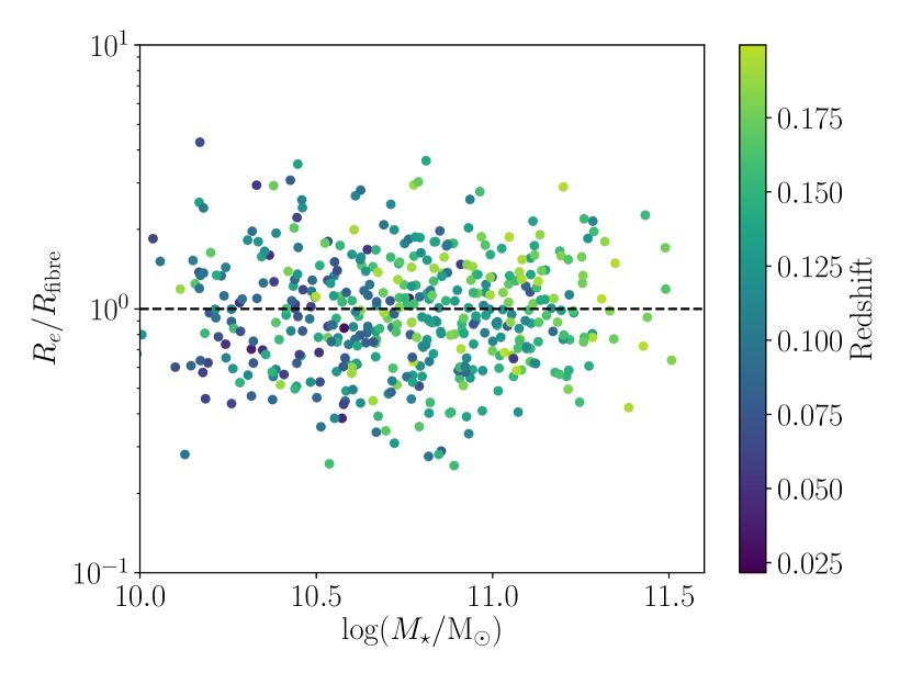
Figure 1: Ratio of effective radius to SDSS fibre size versus stellar mass for the post-coalescence merger sample, with redshift denoted by color. The dashed line indicates $R_{\mathrm{e}}/R_{\mathrm{fibre}}=1$; 55 per cent of post-coalescence merger galaxies fall below this line.

2.1.3 Merger control sample

To construct a control sample for the post-coalescence mergers, we closely follow the control sample selection methodology of Ellison et al. (2013). Explicitly, the overall collection of all possible control galaxies are those that appear to be isolated, having no spectroscopic companion within $80h^{-1}$kpc and with a relative velocity of $\Delta v$ within 10 000 km s^-1. From these galaxies, we then select matching control galaxies for each post-coalescence merger within a redshift tolerance of $\Delta z=0.005$, a mass tolerance of $\Delta\log M_{\star}=0.1$ dex, and a normalized local density difference of $\log(1+\delta_{5})=0.1$ dex. Normalized densities, $\delta_{5}$, are computed relative to the median local environmental density,

$$\Sigma_{n}=\frac{n}{\pi d_{n}^{2}}\,,$$

within $\Delta z\pm 0.01$, where $d_{n}$ is the projected physical distance to the $n$-th nearest neighbour within $\pm 1000$ km s^-1. As in Ellison et al. (2013), we use $n=5$.

We require that there are at least 5 control galaxies per post-coalescence merger. If there are fewer than this, we increase the tolerance limits (additively) by another $\Delta z=0.005$ in redshift, $\Delta\log M_{\star}=0.1$ dex in stellar mass, and $\Delta\log(1+\delta_{5})=0.1$ dex in normalized local density. Only 0.7 per cent of post-coalescence mergers require more than one loop to find more than 5 control galaxies. We end up with $\sim 79~{}000$ control galaxies total.

2.2 Observed post-coalescence merger properties

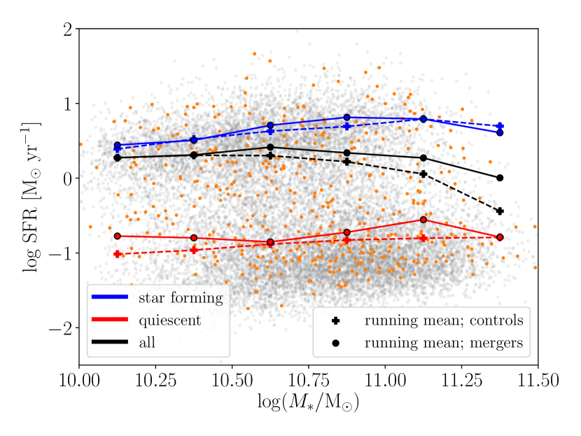
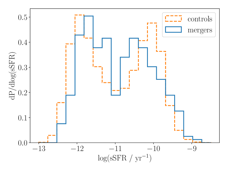
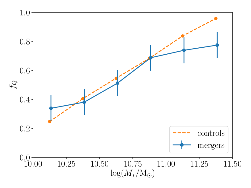
Figure 2: Top: Running average SFR for SDSS post-coalescence mergers (circular points connected by solid lines) and controls (‘+’ symbols connected by dashed lines), broken down by total (black), star forming (blue), and quiescent (red). Each post-coalescence merger’s $\log\mathrm{SFR}-M_{\star}$ value is additionally plotted (small orange points), as is a random subset of the overall SDSS sample (small grey points). Middle: Histograms of the normalized sSFR for post-coalescence mergers (blue solid) and controls (orange dashed). Bottom: Quiescent fraction as a function of stellar mass for the post-coalescence merger sample (blue points connected by a solid line) and our control sample (orange points connected with a dashed line). Errorbars on the mergers are the bootstrapped error on the mean $f_{Q}$; because of the large control sample, errors on the controls’ $f_{Q}$ values are negligible.

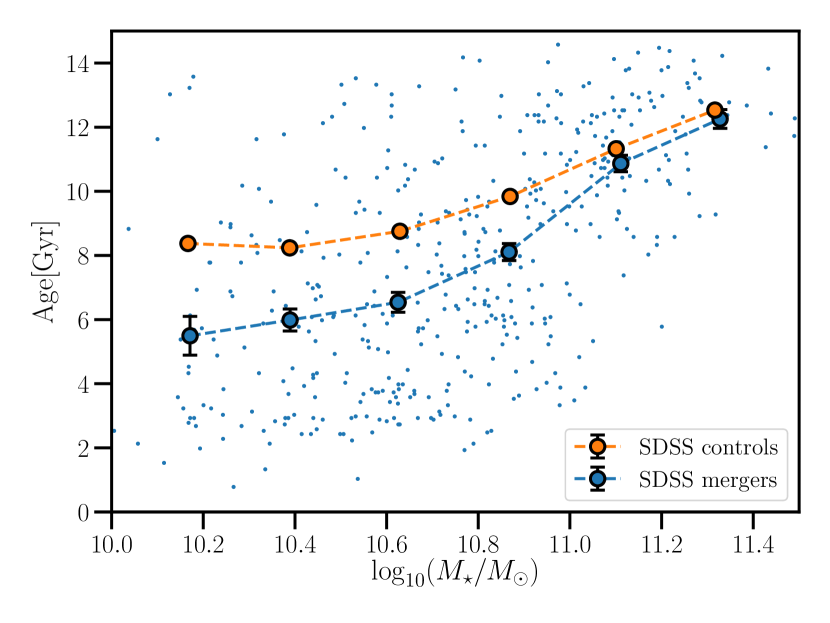
Figure 3: Running mean of the SDSS-derived ages as a function of stellar mass for the merger sample of Bickley et al. (2022) (large blue circles) contrasted with our control sample (orange). Post-coalescence mergers are younger than control galaxies by $\sim 2-3$ Gyr for $10<\log(M_{\star}/\mathrm{M}_{\odot})<11$. Error bars shown are the bootstrapped standard error on the mean. All age–$M_{\star}$ values of the post-coalescence merger sample are shown (small blue points) to give an indication of the scatter in the SDSS ages.

We note some observed properties of the post-coalescence merger sample. In the top subplot of Figure 2, we see that the log of the running mean SFR of the overall post-coalescence merger sample (black) declines less steeply with stellar mass than for the control sample, but only modestly so. By breaking down the sample into star forming (blue) and quiescent (red), using the sSFR division $\log(\mathrm{sSFR})=-0.4\log(M_{\star}/\mathrm{M}_{\odot})-6.6$, we see the difference is primarily due to the increase in SFR of the quiescent post-merger galaxies relative to the control galaxies. This is also clear in the distribution of post-coalescence merger sSFRs shown in the middle subplot. Furthermore, the median star forming merger has a lower sSFR than the median star-forming control. In this sense, the mergers populate the “green valley” to a greater extent than the controls. Nevertheless, because of a small excess of mergers with much higher star formation rates (log sSFR $\gtrsim-9.8$), we still reproduce the mean $\Delta\mathrm{SFR}\sim 0.27$ dex enhancement in star formation rate for star forming galaxies, as measured in Bickley et al. (2022), who used the same post-coalescence merger sample. We additionally note that the fraction of quiescent galaxies is consistent between mergers and controls (bottom subplot), except for the very highest stellar mass bin. The reason for the $\sim 20$ per cent lower quiescent fraction in this stellar mass bin presumably has to do with the enhanced proportion of high sSFR galaxies. As this mass bin is outside of our modeled sample, we do not explore it further in this work.

In Figure 3, we compare the running mean of the post-coalescence mergers (including both quiescent and star forming galaxies) sample with their corresponding control sample. The well-known age-$\log(M_{\star}/\mathrm{M}_{\odot})$ trend (e.g. Nelan et al., 2005; Graves et al., 2007) is apparent for both the post-coalescence mergers and controls sample. The mean age of the post-coalescence merger sample is significantly younger, particularly at lower stellar masses, by up to $\Delta A\sim 3$ Gyr for $\log(M_{\star}/\mathrm{M}_{\odot})\sim 10$. We note that breaking the galaxies down into quiescent or star forming subsets does not change the results, as is expected because Comparat et al. (2017) mask the emission lines (both nebular and AGN) when performing their FIREFLY fitting of the SDSS spectroscopy.

3 Modeling and Results

Our goal is to determine the burst fraction from $1<\mu<10$ mergers by measuring the fraction of the stellar mass from the starburst that can account for the difference in average age as seen in Figure 3. Given the uncertainties on individual observed galaxies’ ages, we only use observed average age differences and model average star formation histories. In other words, we are only looking to model the mean stellar mass burst fraction and the uncertainty on this mean, and will not be modeling the uncertainty for each galaxy in the distribution, which are very difficult to properly characterise. Note that for $\log(M_{\star}/\mathrm{M}_{\odot})>11$, there is no significant age difference, so we restrict the analysis to $10<\log(M_{\star}/\mathrm{M}_{\odot})<11$.

We carry out our modeling by adding a recent burst of star formation to the SFR of the pre-merger progenitors, which we model with a parametric SFH, as described in Section 3.1. We will also need to model the additional star formation during the inspiral phase and so we use published close pair SFR enhancement ratios as a function of pair separation, integrated over inspiral timescales derived from these separations; we present this aspect of the modeling and results in Section 3.2. Finally, in Section 3.3, we present our modeled stellar age results and best-fitting stellar mass burst fraction.

3.1 Control star formation histories

For a set of control galaxy star formation histories, we use functions which are log-normal in time, which have been shown to be excellent fits for individual galaxies for most star formation histories, with the exception being the small fraction of galaxies suddenly quenched shortly after becoming satellites (Diemer et al. 2017; see also Gladders et al. 2013). Following Diemer et al. (2017), we parameterize our control galaxy star formation histories as

$$\mathrm{SFR}_{\mathrm{con}}(t)=\frac{B}{\sqrt{2\pi\tau^{2}}\times t}\exp\bigg{(}-\frac{(\ln(t)-T_{0})^{2}}{2\tau^{2}}\bigg{)}\,,$$ (1)

where $B$, $T_{0}$, $\tau$ are free parameters. We note that our results are robust to the particular choice of parametric SFH, as we discuss in Section 4.1.

We determine $B$ from the total stellar mass of the galaxy we wish to model, i.e. from their equation 2, $M_{\mathrm{final}}=B\times 10^{9}\times f_{\mathrm{ret}}$, where $f_{\mathrm{ret}}=0.6$ is the stellar mass retention factor (similar to that assumed by Gladders et al. 2013 and that found for IllustrisTNG in Diemer et al. 2017).

To solve for the other parameters, we assume the peak time-width relation Diemer et al. (2017) find for their Illustris sample, namely $\sigma_{\mathrm{SFR}}=0.83t^{3/2}_{\mathrm{peak}}$ (their equation 7), where $\sigma_{\mathrm{SFR}}=2t_{\mathrm{peak}}\sinh{\sqrt{2\ln{2}}\tau}$ is the full width at half maximum in linear time for the SFH. Let $A_{\mathrm{con}}$ be the mass-weighted age of the control galaxy. By noting that $t_{\mathrm{peak}}$ is simply the mode of the log-normal distribution, i.e. $t_{\mathrm{peak}}=\exp(T_{0}-\tau^{2}/2)$, and that $t_{\mathrm{now}}-A_{\mathrm{con}}$ is simply the first moment of the distribution, i.e. $t_{\mathrm{now}}-A_{\mathrm{con}}=\exp(T_{0}+\tau^{2}/2)$, we find the following expression that can be solved numerically for $\tau$ using the mass-weighted age as an input:

$$0=0.83(t_{\mathrm{now}}-A_{\mathrm{con}})^{\frac{1}{2}}\exp\bigg{(}\frac{-3\tau^{2}}{4}\bigg{)}-2\sinh(\sqrt{2\ln{2}}\tau).$$ (2)

With $\tau$ now in hand, we can then simply solve for $T_{0}$ using the definition of the first-moment, $t_{\mathrm{now}}-A_{\mathrm{con}}=\exp(T_{0}+\tau^{2}/2)$.

We show example log-normal star formation histories for a range of stellar masses, $10<\log(M_{\star}/\mathrm{M}_{\odot})<11$, as the solid smooth curves in Figure 4, using the SDSS control galaxies’ age–$M_{\star}$ relation in Figure 3 to solve for the SFH parameters for each stellar mass shown.

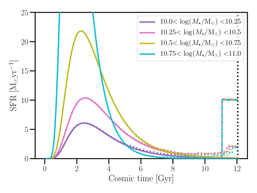
Figure 4: Mean log-normal control galaxy star formation histories (solid lines) overlaid with estimated enhanced SFR due to inspiral (dashed lines) binned by stellar mass, as well as an example $\Delta t_{\mathrm{burst}}=1$ Gyr additive SFR burst of $\mathrm{SFR}_{\mathrm{burst}}=10~{}\mathrm{M}_{\odot}$yr^-1. Enhanced SFR from the inspiral phase was calculated using the SFR-$r_{p}$ galaxy pair results of Patton et al. (2013), with radii converted to average inspiral timescales using Equation 3.2. Note that star formation histories in this figure are shown up until the average observed redshift, $t_{\mathrm{merge}}(z=0.13)\sim 12$ Gyr.

Since we will be modifying these control star formation histories for our merger analysis, rather than use the input stellar mass and age for a given star formation history, we numerically integrate the star formation history. The stellar masses of a galaxy at the average observed redshift of $z=0.13$, is calculated as

$$M_{\star}(t_{\mathrm{now}}) =\int_{0}^{t_{\mathrm{now}}}\frac{\mathop{}\!\mathrm{d}M_{\star}}{\mathop{}\!\mathrm{d}t}\mathop{}\!\mathrm{d}t$$ (3)

$$=f_{\mathrm{ret}}\int_{0}^{t_{\mathrm{now}}}\mathrm{SFR}(t)\mathop{}\!\mathrm{d}t,$$ (4)

where $t_{\mathrm{now}}=12.05$ Gyr. Similarly, ages are calculated as

$$A_{\mathrm{con}} =t_{\mathrm{now}}-\frac{1}{M_{\star}(t_{\mathrm{now}})}\int_{0}^{t_{\mathrm{now}}}t\Big{(}\frac{\mathop{}\!\mathrm{d}M_{\star}}{\mathop{}\!\mathrm{d}t}\Big{)}\mathop{}\!\mathrm{d}t$$ (5)

$$=t_{\mathrm{now}}-\frac{f_{\mathrm{ret}}}{M_{\star}(t_{\mathrm{now}})}\int_{0}^{t_{\mathrm{now}}}t\,\mathrm{SFR}(t)\mathop{}\!\mathrm{d}t\,;$$ (6)

we note it is written this way since it is a mass-weighted age, which is expressed as a lookback time.

3.2 SFR enhancement during the inspiral phase using close pairs

Previous studies have shown that star formation in the close pair “inspiral” phase of the merger is enhanced, as summarised, for example, in table 1 of Behroozi et al. (2015). To compute the increase in stellar mass during inspiral, we use the empirically-determined relative enhancement in SFR (a ratio to control galaxies) vs $r_{p}$ relation from figure 1 of Patton et al. (2013). We convert the projected separation bins to merging timescales by assuming galaxies at a given radius will take some increment of time to fall from one $r_{p}$ bin to the next, $dt_{i}=t_{i+1}-t_{i}$, where $t_{i}$ is the average infall time for some $r_{p}$ bin and $t_{i+1}$ is the average infall time for the next farthest $r_{p}$ bin. The average infall time for a given bin, $r_{p,i}$ is given by $t_{i}=t_{\mathrm{merge}}(r_{p,i})$, where

$$t_{\mathrm{merge}}(r_{p})=2.2~{}\mathrm{Gyr}\frac{r_{p}}{50~{}\mathrm{kpc}}\Bigg{(}\frac{\mu}{4}\Bigg{)}\Bigg{(}\frac{M_{\star}}{4\times 10^{10}h^{-1}\mathrm{M}_{\odot}}\Bigg{)}^{-0.3}\Bigg{(}1+\frac{z}{8}\Bigg{)},$$

which is adapted from equation 10 of Kitzbichler & White (2008) with an extra multiplicative term $\mu$ as found in the fit relation from Jiang et al. (2014), normalized to $\mu=4$. The extra term is included to correct for Kitzbichler & White (2008) not examining the dependence of merging time on a pair’s mass-ratio (this led to their original expression only matching that of Jiang et al. (2014) for $\mu=4$), which is a significant effect. We note that the mean $\mu$ depends weakly on stellar mass (using only the range $1<\mu<10$), decreasing from $\mu=3.25$ to $\mu=2.8$ from $\log(M_{\star}/\mathrm{M}_{\odot})\sim 10$ to $\log(M_{\star}/\mathrm{M}_{\odot})\sim 11$.

Whether we compute $t_{\mathrm{merge}}$ using the mean $\mu$ for a given stellar mass bin or whether we calculate the mean $t_{\mathrm{merge}}$ for a whole distribution of observed pair $\mu$ values does not impact our results. We find that for 2/3 of pairs $t_{\mathrm{merge}}<1$ Gyr.

The excess stellar mass from the inspiral phase prior to merging is then

$$\Delta M_{\star}=f_{\mathrm{ret}}\sum_{i}\Delta~{}\mathrm{SFR}_{i}\times\mathrm{SFR}_{\mathrm{con}}(t_{i})dt_{i},$$

where $\Delta~{}\mathrm{SFR}_{i}$ is the ratio in star formation rate between galaxies that are close pairs and their corresponding controls. $\mathrm{SFR}_{\mathrm{con}}$ is simply the mean SFR of an SDSS galaxy with the control galaxy’s stellar mass. The result from this choice is robust as long as most of an inspiral’s excess star formation occurs in the last few Gyr, which we will shortly show. We again assume $f_{\mathrm{ret}}=0.6$.

In Figure 4, we illustrate the effect of this additional star formation on the overall modeled star formation history due to the inspiral phase (dotted line). Most importantly for this work is the impact on stellar ages from the inspiral phase, which we show with black arrows in the subplots in Figure 5. The enhanced star formation results in younger stellar ages for galaxies, with the effect largest ($\sim 1.5$ Gyr) for the lowest stellar mass bin ($10<\log(M_{\star}/\mathrm{M}_{\odot})<10.25$), and smallest ($\sim 0.6$ Gyr) for the highest stellar mass bin ($10.75<\log(M_{\star}/\mathrm{M}_{\odot})<11)$. Interestingly, this removes the trend in $\Delta A$ with stellar mass, leaving $\Delta A\sim-1.4$ Gyr at all considered stellar mass bins to be explained by a starburst during coalescence.

3.3 Starburst during coalescence

We can explain the remaining difference in stellar ages via a simple star-formation burst during coalescence, i.e. upon two galaxies merging. To do this, we model the enhanced star formation during coalescence as an additive burst with a flat SFR, parametrized by the duration of the burst, $\Delta t_{\mathrm{burst}}$, and the burst fraction for the resulting merged object, $f_{\mathrm{burst}}\equiv(M_{\star,\mathrm{merger}}-M_{\star,\mathrm{con}})/M_{\star,\mathrm{merger}}$. $M_{\star,\mathrm{con}}$ is the mass of the two merged galaxies without a burst (where ‘con’ is short for ’control’), and $M_{\star,\mathrm{merger}}$ is the final merged object with the burst. We illustrate a simple example $\Delta t_{\mathrm{burst}}=1$ Gyr long burst of $\mathrm{SFR}=10~{}\mathrm{M}_{\odot}\mathrm{yr}^{-1}$ in Figure 4.

This modeling requires an iterative computation to find the input control galaxy’s stellar mass. Since our SFH model for control galaxies takes in age as an input, to estimate an age for a trial control galaxy given some stellar mass, we fit the mean age–$M_{\mathrm{\star}}$ relation for controls with a tight-fitting fourth-order polynomial and flat relation below $x=\log(M_{\star}/\mathrm{M}_{\odot})=10.2$. We put in a flat trend instead of the polynomial for the lower stellar mass end as there are few post-coalescence mergers (and therefore few matched controls) below $\log(M_{\star}/\mathrm{M}_{\odot})\sim 10.2$ and the overall trend for SDSS galaxies is approximately flat below this. We iterate through control masses (the stellar mass of the merged galaxies without the starburst added) until we find the needed control stellar mass to give the desired burst fraction.

For our model, we plot the change in age, $\Delta A=A_{\mathrm{merger}}-A_{\mathrm{con}}$ as a function of $f_{\mathrm{burst}}$ for our four stellar mass bins in Figure 5. For each stellar mass bin we additionally plot the measured difference in age between the post-coalescence mergers and control sample as a horizontal (grey) band, shifted by the modeled inspiral $\Delta A$ results of the previous section.

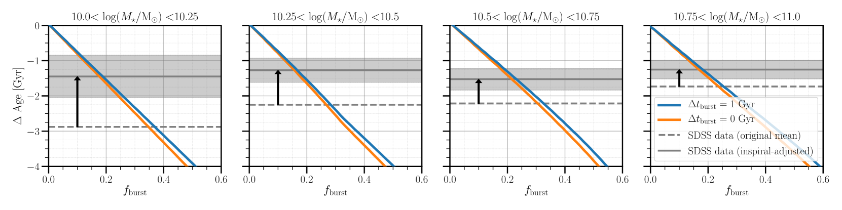
Figure 5: Change in modeled merger age, $\Delta A=A_{\mathrm{merger}}-A_{\mathrm{con}}$, relative to a control galaxy as a function of burst fraction, $f_{\mathrm{burst}}=(M_{\mathrm{merger}}-M_{\mathrm{con}})/M_{\mathrm{merger}}$, for four stellar mass bins. On each subplot we show two models: one with an instantaneous burst ($\Delta t_{\mathrm{burst}}=0$ Gyr) and a model using $\Delta t_{\mathrm{burst}}=1$ Gyr. In solid grey we plot the mean $\Delta A$ from the SDSS data shifted by the modeled inspiral phase using close pairs data (black arrow indicates the shift), with the shaded region indicating the bootstrapped error on the mean.

Earlier works find short star formation bursts. For example (Di Matteo et al., 2008) find bursts of up to 500 Myr long at most, with average durations of 200–300 Myr. With this in mind, we show two models with burst durations of $\Delta t_{\mathrm{burst}}=0$ Gyr (instantaneous; blue line) and $t_{\mathrm{burst}}=1$ Gyr (long duration extreme case; orange line), which display nearly identical linear declining trends, with a maximum difference between the $\Delta A$ of the two models of $\sim 0.5$ Gyr for high burst fractions, as expected from the difference in age of the two bursts. Additionally, if we perform a simple back-of-the-envelope calculation for an instantaneous burst and assume the control stellar mass is simply the same as the merger, i.e. $f_{b}=(A_{\mathrm{merger}}-A_{\mathrm{con}})/A_{\mathrm{merger}}$, then we would expect that $\Delta A=-A_{\mathrm{con}}f_{\mathrm{burst}}$, which is a very similar linear trend in $\Delta A$ as a function of $f_{\mathrm{burst}}$ to our plotted $\Delta t_{\mathrm{burst}}=0$ Gyr model.

Assuming the uncertainties on the SDSS ages are normally distributed, we compute the best-fitting $f_{\mathrm{burst}}$ with uncertainties in each stellar mass bin, which we show in Figure 6 for both models. There is a small systematic offset in best-fitting $f_{\mathrm{burst}}$, such that the $\Delta t_{\mathrm{burst}}=1$ Gyr is higher by $\sim 0.02$, a difference which is significantly smaller than the uncertainties. We find no trend in $f_{\mathrm{burst}}$ with stellar mass. The mean stellar mass fraction across our four stellar mass bins is $f_{\mathrm{burst}}=0.18\pm 0.02$ ($f_{\mathrm{burst}}=0.19\pm 0.03$ for $\Delta t_{\mathrm{burst}}=1$ Gyr).

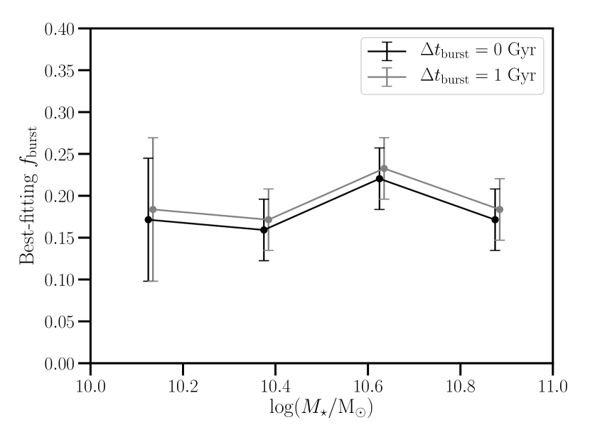
Figure 6: Best-fitting burst fraction, $f_{\mathrm{burst}}=(M_{\mathrm{merger}}-M_{\mathrm{con}})/M_{\mathrm{merger}}$ (for an instantaneous burst), as a function of stellar mass. We show both models from Figure 5: the one with an instantaneous burst ($\Delta t_{\mathrm{burst}}=0$ Gyr) and a model using $\Delta t_{\mathrm{burst}}=1$ Gyr.

4 Discussion

The inspiral phase of galaxy mergers has received significant attention in the literature, in both observational and simulation work, thanks to the ease of observationally identifying close pairs. Since post-coalescence mergers have received relatively little focus in observational work, we focus our discussion primarily on our modeled starburst at the time of coalescence.

4.1 Robustness of measured burst fraction

In this section we explore the robustness of our measured stellar mass burst fraction. In particular, we check, in turn, the effects of the SDSS fibre aperture, the impact of choosing the whole post-coalescence merger sample versus only quenched galaxies, and whether our modeling is sensitive to choice of star formation history.

As noted earlier, the mean redshift of the merger sample is 0.13, for which the SDSS fibres cover a radius of 3.6 kpc. Since the stellar burst is likely mainly in the central regions of the galaxy, most of the burst should fit within the fibre, but some of the galaxy’s non-nuclear stellar mass may be cut off. In Figure 1, we found that $R_{\mathrm{e}}/R_{\mathrm{fibre}}\sim 1$ for an average galaxy in our sample, with little dependence on stellar mass. This implies that for the large majority of galaxies there is no impact on our results, within the margin of error. Additionally, Yoon et al. (2023) studied elliptical galaxies with tidal features (see Section 4.3) and found no difference in the mass fraction formed in the last $2.5$ Gyr, when this was measured within apertures $R<R_{\mathrm{e}}$ compared with apertures $R>R_{\mathrm{e}}$. Their results indicate that even if we relax our assumption that the recently-formed stellar mass is centrally concentrated, there is no significant impact on our results from the limited fibre size employed by SDSS.

The merger and control samples have no restrictions on their observed SFRs. For those post-coalescence mergers that are still forming stars at the time at which they are observed, one might expect them to continue doing so for some time after. In that case, the observed burst fraction may underestimate the final burst fraction. This can be checked by using only quiescent galaxies in the analysis. However, restricting to only quiescent galaxies reduces our post-coalescence merger sample from 442 galaxies to 258, with very few galaxies remaining below $\log(M_{\star}/\mathrm{M}_{\odot})<10.5$. For the full stellar mass range we find $f_{\mathrm{burst}}=0.16\pm 0.04$, with a higher value of $0.24\pm 0.04$ for $\log(M_{\star}/\mathrm{M}_{\odot})>10.5$, both consistent with our best-fitting value of $f_{\mathrm{burst}}=0.18\pm 0.02$ for the full sample including both star forming and quiescent galaxies.

We expect our modeling results to be robust to changes in the SFH, as long as the control SFH results in the correct control galaxy stellar mass and age. As a test of the robustness of our best-fitting burst fractions to the choice of SFH, we replace our controls’ log-normal SFH with a delayed-tau SFH model,

$$\mathrm{SFH}_{\mathrm{con}}(t)=\begin{cases}B\exp\big{(}-\frac{t-t_{i}}{\tau}\big{)},&t\geq t_{i}\\ 0,&t<t_{i},\end{cases}$$ (7)

where $B=M_{\star,\mathrm{con}}/(10^{9}f_{\mathrm{ret}}\tau$) normalizes the star formation history to give the control galaxy’s stellar mass. We set $t_{i}=1$ Gyr as suggested by Simha et al. (2014), and $\tau$ is chosen such that we reproduce the SDSS controls’ age.

Using the delayed-$\tau$ SFH instead of a log-normal SFH results in a lower modeled post-coalescence merger $\Delta A$ by up to 0.09 Gyr, or a lower $f_{\mathrm{burst}}$ by up to 0.01, for a given value of $f_{\mathrm{burst}}$ or $\Delta A$, respectively. This effect is greatest for the lower stellar mass bins and negligible for the highest stellar mass bin. From this test it is clear that swapping out our original SFH model with delayed-$\tau$ has no significant impact on our conclusions. We expect this to hold for any reasonable choice of parametric SFH.

4.2 Dependence on the merger progenitors

Unlike close pairs, with post-coalescence mergers it is impossible to identify the masses, morphological types, and gas fractions of the progenitors of an individual merger. This problem can be studied statistically, however.

The CNN used to identify the post-coalescence merger sample was trained with merger mass ratios, $1<\mu<10$, with $\overline{\mu}\sim 3$. What remains uncertain, however, is whether the visual-confirmation step is biased to mass ratios closer to unity. Quantifying this possible effect would require extensive human examination of the mock training set, a rather infeasible task. In any case, our stellar mass burst fraction is not especially sensitive (compared to the uncertainties) to modest changes in the mean $\mu$ (e.g. if $\overline{\mu}\sim 2$ or $\overline{\mu}\sim 4$, rather than $\overline{\mu}\sim 3$).

We note that for a post-coalescence merger galaxy with $\log(M_{\star}/\mathrm{M}_{\odot})\sim 10.2$ with a 20% burst of stars one might then expect the progenitors to have stellar masses of $\log(M_{\star}/\mathrm{M}_{\odot})\sim 10.0$ and 9.5. These would typically be gas-rich, star-forming galaxies in the “blue cloud” and so the merger would be gas-rich or “wet”. Once the progenitors have stellar masses above $\log(M_{\star}/\mathrm{M}_{\odot})\sim 10.5$, the probability that they will be gas rich drops rapidly. Thus for post-merger remnants with $\log(M_{\star}/\mathrm{M}_{\odot})\gtrsim 10.7$, we expect the burst fraction to drop rapidly as these mergers become “dry”. Indeed, as shown in Figure 3, for $\log(M_{\star}/\mathrm{M}_{\odot})>11$, the age difference between mergers and controls is consistent with zero (and hence so is the burst fraction).

4.3 Comparison to other burst fractions in the literature

Most prior work modeling the stellar mass created in a merger starburst have been in complex hydrodynamical simulations or semi-analytic models, but a few works derive stellar mass burst fractions directly from observations of post-coalescence mergers.

In particular, Yoon et al. (2023) use FIREFLY to fit star formation histories to MaNGA integral field unit spectroscopic data of 193 early-type galaxies (ETGs; visually identified using the SDSS $g$, $r$, and $i$ band imaging), 44 of which ($23$ per cent) display tidal features (see Yoon & Lim, 2020, for sample selection). Tidal features were identified visually in the coadded imaging of the Stripe 82 region of SDSS, which is $\sim 2$ mag. deeper than the rest of SDSS (UNIONS is in turn $\sim 0.3$ mag. deeper than Stripe 82). They found that ETGs with tidal tail features have younger stellar ages than those without by $1-2$ Gyr for our stellar mass range, shorter than the $2-3$ Gyr we see between post-coalescence mergers and controls.

They find the fraction of stellar mass formed in ETGs with tidal features in the past $2.5$ Gyr is $2\pm 1$ and $7\pm 3$ percent higher than those without, at $10<\log(M_{\star}/\mathrm{M}_{\odot})\leq 10.6$ and $10.6\leq\log(M_{\star}/\mathrm{M}_{\odot})\leq 11.1$, respectively. The fraction of stellar mass which was formed in the previous $2.5$ Gy (which includes inspiral) that they find for ETGs with tidal features is only $13\pm 3$ per cent and $5\pm 1$ per cent, for $10<\log(M_{\star}/\mathrm{M}_{\odot})\leq 10.6$ and $10.6\leq\log(M_{\star}/\mathrm{M}_{\odot})\leq 11.1$, respectively. They find the same fractions when measuring either within $R<R_{\mathrm{e}}$ and within $R>R_{\mathrm{e}}$, meaning we should be able to compare with their result directly. As well, we note that our result is robust to whether we use our entire sample or only quenched galaxies.

Their stellar mass burst fraction is substantially lower than the burst fractions that we find, possibly due to a few important factors. Selecting only for ETGs may bias towards galaxies that have less cold gas than our sample which may contain a proportion of disc galaxies (discs can re-form post-merger, e.g. Hopkins et al., 2008b). However, we find that our results do not change when we consider only quenched galaxies. Including faint tidal features in their selection may also bias the sample towards minor mergers, which are much more common than major mergers. Finally, whereas the sample we use is primarily of recent post-coalescence mergers, Yoon et al. (2023) selected on generic tidal features, and these may include all stages of the merger process from small satellites stretched out into a tidal stream after first pericentre to $\sim 3$ Gyr after coalescence (although see also Desmons et al., 2023, who suggest galaxies selected by tidal features alone are mostly post-coalescence mergers).

Hopkins et al. (2008b) studied morphologically-identified gas-rich merger candidates from Rothberg & Joseph (2004) and fitted surface brightness profiles to quantify the excess central light created by a recent starburst(s). 40 out of 52 of the galaxies are classified as fully violently relaxed in Rothberg & Joseph (2004), although our conclusion from their result is not changed whether we include/exclude those with relaxation classified as ‘incomplete’. In other words, their sample and result should be representative of recently coalesced gas-rich mergers. They find an average best-fitting excess light fraction of $f_{e}=0.25\pm 0.03$ for galaxies with $\log(M_{\star}/\mathrm{M}_{\odot})\sim 11$, consistent with our burst fraction of $0.18\pm 0.04$ at this stellar mass (including the inspiral period of $\sim 0.01$). Systematic factors such as overestimation of burst mass to burst light fraction, due to reliance on one photometric band, may have resulted in modest overestimation of the stellar mass burst fraction.

French et al. (2018) perform detailed SED-fitting and modeling of post-starburst galaxies, objects for which a substantial fraction appear to be post-coalescence mergers (e.g. Sazonova et al., 2021; Ellison et al., 2022; Wilkinson et al., 2022). We note that post-starburst galaxies are only a minority ($\sim 20$ per cent) of our post-coalescence merger sample (Ellison et al., 2022). Therefore, it is perhaps not surprising that they find a much higher mean burst stellar mass fraction of $\sim 0.5$ for $\log(M_{\star}/\mathrm{M}_{\odot})\sim 10$ galaxies (versus our $0.28\pm 0.07$ value including the inspiral period). For more massive galaxies with $\log(M_{\star}/\mathrm{M}_{\odot})>10.5$ their burst stellar mass fraction of $0.21\pm 0.02$ is consistent with ours.

It is also interesting to compare our results with the predictions from hydrodynamical simulations. The IllustrisTNG hydrodynamical simulation was used to train the CNN used by Bickley et al. (2022) to identify the post-coalescence mergers used in our work. Hani et al. (2020) examined post-coalescence merger galaxies in IllustrisTNG and found a modest $\sim 2$ factor increase in SFR, which quickly declines, resulting in only a small $f_{\mathrm{burst}}\sim 0.5$ per cent. Their result is in clear contradiction with ours and the papers discussed above, apart from Yoon et al. (2023). Moreno et al. (2019) used the Feedback in Realistic Environments 2 (FIRE-2) hydrodynamical simulations to study pairs of merging galaxies at a 1 pc resolution. Star formation becomes enhanced around the time of first pericentre, followed by a significant (mostly central) starburst with $\mathrm{SFR}\sim 10~{}\mathrm{M}_{\odot}\mathrm{yr}^{-1}$ beginning at second pericentre, $\lesssim 250$ Myr prior to coalescence. Integrating the excess SFR for their $3\times 10^{10}~{}\mathrm{M}_{\odot}$ and $1.2\times 10^{10}~{}\mathrm{M}_{\odot}$ simulated progenitor galaxies (combined stellar mass of $\log(M_{\star}/\mathrm{M}_{\odot})\sim 10.6$), we find 5 per cent of the post-coalescence merger’s final stellar mass comes from the inspiral period (prior to second pericentre) and 8 per cent from the burst. This is consistent with our inspiral period’s excess stellar mass fraction, but less than half of our best-fitting stellar mass burst fraction for the starburst.

4.4 Starburst duration

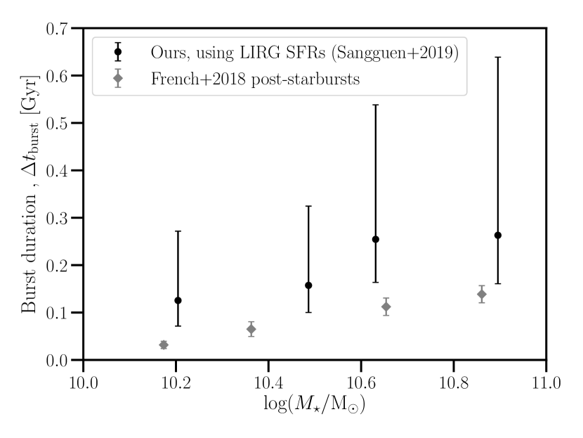
Figure 7: Estimated starburst duration, $\Delta t_{\mathrm{burst}}$, as a function of stellar mass, estimated by assuming $f_{\mathrm{burst}}$ from Figure 6 (black points) and the ‘late-stage’ inspiraling LIRG SFRs from Shangguan et al. (2019) (a presumed population of starburst galaxies).

We can constrain the duration of the starburst during coalescence, if the typical SFR during the starburst is known. Luminous infrared galaxies (LIRGs, Sanders & Mirabel, 1996) are believed to be starburst galaxies, with $\mathrm{SFR}>10~{}\mathrm{M}_{\odot}$yr^-1 (similar SFRs to a typical starburst sample, French et al., 2018), usually inferred from IR luminosity (although we note that in principle AGN could be contributing to this, e.g. Iwasawa et al., 2011; Petric et al., 2011). As described earlier, the vast majority of low-$z$ starburst/post-starburst galaxies may be due to mergers (see Section 1). LIRGs/ULIRGs have substantial young stellar populations ($\leq 100$ Myr), and appear to have gone through a period of enhanced star formation prior to their current burst. There is also some correlation with being late-stage inspiraling pairs and especially with coalescing/coalesced merger galaxies (e.g. Gao et al., 1997; Rodríguez Zaurín et al., 2010; Stierwalt et al., 2013; Larson et al., 2016).

Because of the likelihood at least the majority of LIRGs are due to mergers, we use a sample of 52 late-stage inspiraling LIRGs’ SFRs from Shangguan et al. (2019) to measure the typical merger SFR and so constrain the starburst duration. We choose the subset of these morphologically identified by Stierwalt et al. (2013) as having two nuclei in a common envelope.

We fit a power-law to the $\mathrm{SFR}$–$M_{\star}$ trend for this subset of objects (see objects labeled ‘(d)’, e.g. in their figure 5), finding $\mathrm{SFR}=(29\pm 13)M_{\star}^{0.53\pm 0.17}$. Since our modeled burst fraction result is quite insensitive to choice of $\Delta t_{\mathrm{burst}}$, we can constrain the burst duration

$$\Delta t_{\mathrm{burst}} =\frac{\Delta M_{\star}}{f_{\mathrm{ret}}\times\mathrm{SFR_{\mathrm{LIRGs}}}}.$$ (8)

We show the result of this calculation in Figure 7. We see $\Delta t_{\mathrm{burst}}\sim 120$ Myr for the lowest stellar mass bin, increasing to $\Delta t_{\mathrm{burst}}\sim 250$ Myr for the highest stellar mass bins, albeit with large uncertainties from the LIRG SFR–$M_{\star}$ relation. We note our burst times are similar to the free-fall or violent relaxation time at the outer edge of the disk.

French et al. (2018), who studied post-starburst galaxies, found an average duration of $103\pm 23$ Myr for $10<\log(M_{\star}/\mathrm{M}_{\odot})<11$ galaxies. Their starburst duration increases with stellar mass, from $30$ Myr for $\log(M_{\star}/\mathrm{M}_{\odot})\sim 10$ to $140$ Myr for $\log(M_{\star}/\mathrm{M}_{\odot})\sim 11$, and is systematically shorter than our estimate, as shown in Figure 7. By construction, PSBs are selected to have strong spectral signatures of a burst, whereas the sample we’ve used is morphologically-selected to have post-coalescence merger features, regardless of whether there was a burst or not. This likely explains the difference in intensity and duration of starburst between the sample used by French et al. (2018) and that used by this work.

Hani et al. (2020) trace their Illustris TNG100-1 $\log(M_{\star}/\mathrm{M}_{\odot})>10$ simulated post-coalescence merger sample forward in time and find that significant enhancements in SFR last for $100-250$ Myr post-coalescence (with uncertainty coming from the 162 Myr temporal resolution for the simulation), with a total decay time of $\sim 0.5$ Gyr for this enhancement. This effect was independent of the merger mass ratio. Their timescale is consistent with our estimate. Their SFR burst peaks at a factor only $\sim 2$ higher than their control galaxy, much lower than the factors of 40 – 100 seen in LIRGs. In the higher resolution FIRE-2 merger simulations, Moreno et al. (2019, 2021) find a longer burst duration than we do: 0.5 Gyr (beginning at second pericentre and therefore finishing 250 Myr after coalescence) for their $\log(M_{\star}/\mathrm{M}_{\odot})\sim 10.6$ simulated merger.

4.5 Is there enough cold gas to fuel the burst?

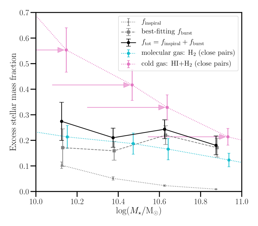
Figure 8: Comparison of estimated stellar mass burst fractions from our modeling of the inspiral phase (small grey circles), best-fitting $f_{\mathrm{burst}}$ (grey squares), and the total excess stellar mass from these two contributions (black points). Also shown are molecular (blue diamonds) and total cold gas (pink circles) converted into the equivalent mass fraction of long-lived stars by multiplying by $f_{\mathrm{ret}}=0.6$. Pink arrows show the stellar mass shift for close pairs gas fractions (so they can be compared to post-coalescence merger quantities), which is applied to both molecular and atomic gas; see text for details.

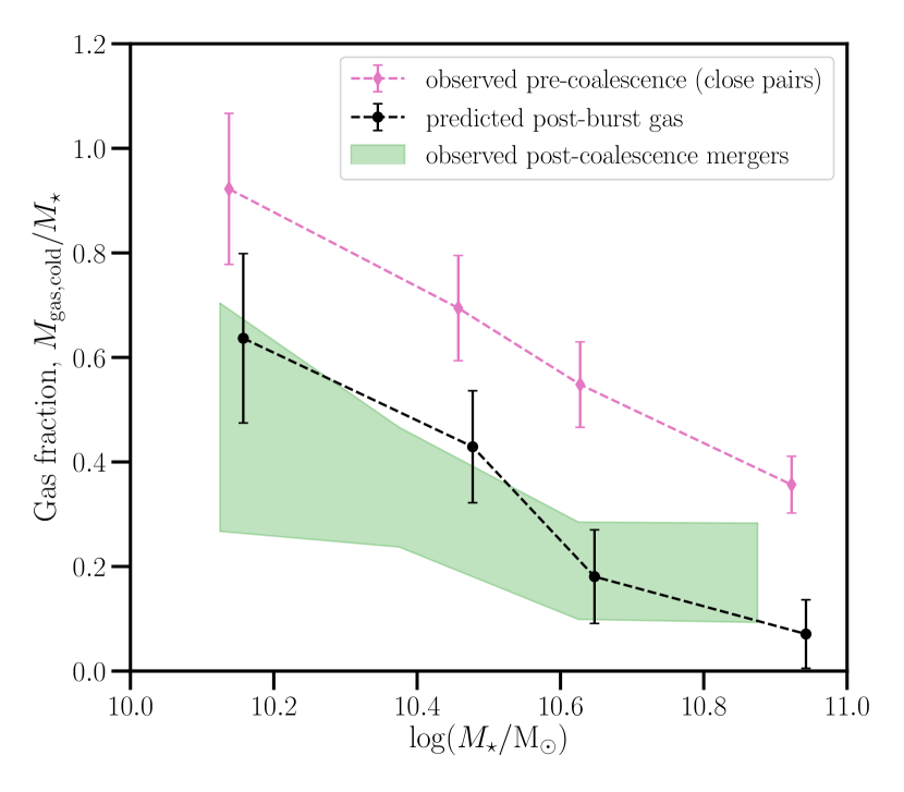
Figure 9: Comparison of cold gas before (pink points) and after coalescence (green), as well as our prediction for remaining cold gas after the burst (black points), all as a fraction of the final merger stellar mass. Our prediction is simply the cold gas before minus the gas consumed during star formation (any gas ejected in supernovae is assumed to be hot). For the post-coalescence mergers we use the H I  gas masses from Ellison et al. (2018) and $\mathrm{H_{2}}$ gas masses from various samples of post-starburst galaxies (French et al., 2015; Rowlands et al., 2015; Otter et al., 2022, see text for details).

The general picture of cold gas in mergers is as follows. Atomic gas in the galaxy outskirts flows inwards, due to decreased angular momentum from gravitational torques, resulting in rapidly increased cold gas density in the central region. This cold atomic gas condenses into molecular clouds, with collision-induced pressure possibly accelerating the formation of additional molecular gas from atomic (H I ) gas (Moster et al., 2011). This additional molecular gas in the core then leads to intense star formation in the galaxy nucleus (Mihos & Hernquist, 1996; Di Matteo et al., 2008; Renaud et al., 2014). Turbulence induced by gravitational torques during interactions, particularly at the start of coalescence, may also lead to gas fragmentation, forming massive and dense molecular clouds, fueling the intense star formation of a starburst (see e.g. Teyssier et al., 2010; Bournaud et al., 2011).

Such a picture is seen in detailed hydrodynamical simulations. In the FIRE-2 simulations, Moreno et al. (2021) find a $0.8$–$1$ dex enhancement of cool atomic and $1.1$–$1.2$ dex enhancement of cold-dense molecular gas mass in the central regions ($r<1$ kpc) at time of second pericentre, coming from the galaxy outskirts ($r=1$–10 kpc). This excess gas in the central region rapidly declines, back to the baseline of the two galaxies evolving in isolation, during the duration of the starburst ($\sim 0.5$ Gyr).

A key question is then whether there is enough cold gas fuel available to form the excess mass of stars formed, namely $\sim 0.2M_{\star,\mathrm{merger}}$, and if so, how much gas remains after the burst? To examine this question, we look at cold gas measurements for pairs of galaxies to estimate the amount of cold gas available to form stars at the start of coalescence.

We take cold gas fraction measurements of H I  and H₂ from the XCOLD GASS survey (as presented in Saintonge et al., 2017), a systematic survey of $0.01<z<0.05$ galaxies selected from SDSS to be representative down to $10^{9}\mathrm{M}_{\odot}$ in stellar mass. We then adjust these gas masses by the relative enhancements in the proportions of the cold gas components for close pairs. In particular, we note that H I  does not appear significantly different from controls in recent samples of several dozen pair galaxies, with some debate as to the exact impact (Ellison et al., 2015; Yu et al., 2022). For pre-coalescence H I  gas masses, we simply use the unmodified Saintonge et al. (2017) H I  masses. For $\mathrm{H_{2}}$, we take the $\mathrm{H_{2}}$ gas mass enhancements, relative to controls, of very close pairs from Pan et al. (2018) (most have stellar mass ratios $1\leq\mu\leq 10$) and we multiply their figure 8 value (projected separation $r_{p}<30$ kpc) by the ratio of gas masses for $10<\log(M_{\star}/\mathrm{M}_{\odot})<11$ galaxies to their whole sample, to find a mean molecular gas fraction ($M_{\mathrm{H_{2}}}/M_{\star}$) enhancement of $0.62\pm 0.07$ dex (see also Casasola et al., 2004; Violino et al., 2018). Such an enhancement increases the $\mathrm{H_{2}}$ mass fraction of the cold gas from $M_{\mathrm{H_{2}}}/(M_{\text{H\scalebox{0.8}{I}}}+M_{\mathrm{H_{2}}})=0.08\textnormal{ -- }0.11$ for the general field sample of Saintonge et al. (2017) to $M_{\mathrm{H_{2}}}/(M_{\text{H\scalebox{0.8}{I}}}+M_{\mathrm{H_{2}}})=0.39\textnormal{ -- }0.58$ for close pairs (with higher gas fractions in these given ranges being for lower stellar mass galaxies). We note their result is consistent with Lisenfeld et al. (2019), when this latter work is corrected to account for He and metals. Such a large increase in molecular gas during the inspiral process is also consistent with data from LIRGS that are morphologically-defined as having double nuclei in the pre-coalescence stage of merging (Larson et al., 2016).

The relevant gas fraction for a merger involves not the stellar mass of the final merger product but rather the gas fractions expected from the progenitors and summed together appropriately. The final stellar mass is then the sum of the stellar masses of the progenitors (close pairs) plus the retained stellar mass after the cold gas is converted to stars. To compare gas fractions with the stellar mass burst fraction, we therefore shift the stellar mass bins of the gas fractions by doubling their mass and appropriately adding in the stellar mass burst, i.e. $M_{\star}^{\prime}=2M_{\star}/(1-f_{\mathrm{burst}})$. We note that whether we assume equal mass mergers or a more realistic e.g. $\mu=3$, the impact on the gas fractions for our stellar mass range is negligible. We show these gas fractions overlaid with our best-fitting $f_{\mathrm{burst}}$ values in Figure 8. Assuming $f_{\mathrm{ret}}=0.6$, we find there is just enough molecular gas available prior to coalescence to form the stellar mass burst, but only if either there is $\sim 100$ per cent efficiency in converting existing molecular gas to stars or if more molecular gas is formed during coalescence. Using instead the total cold gas content (molecular and atomic) prior to coalescence, the gas consumption efficiency of $e=(f_{\mathrm{burst}}M_{\star,\mathrm{merger}}/f_{\mathrm{ret}})/M_{\mathrm{gas,cold}}$ ranges from 30–80 per cent, increasing in efficiency from the lowest to highest stellar mass bin.

A similar comparison has been performed for post-starburst galaxies. In particular, French et al. (2018, see also ) find a significant decline in molecular gas to stellar mass fraction with increasing post-burst age, which persists after controlling for fraction of stellar mass produced in the recent burst. Assuming an exponentially declining gas fraction, they find a best-fitting timescale of $117-230$ Myr and best-fitting initial molecular gas fractions of 0.4–0.7 at a post-burst age of zero (lower end of this range is consistent with Pan et al., 2018). Based on their fit relation, for a post-starburst about $0.5$ Gyr after the beginning of the burst (their mean found for post-starbursts with SED fitting), a post-starburst has $M_{\mathrm{\mathrm{H}_{2}}}/M_{\star}\sim 0.05$. The difference between their results and ours is likely driven by the difference in sample selection, since as noted earlier, only $\sim 20$ per cent of post-coalescence mergers are post-starbursts (Ellison et al., 2022).

Subtracting the gas consumed in the burst from the total expected cold gas fraction in the merging pair pre-coalescence, we predict a residual post-burst cold gas fraction as shown in Figure 9 (black points). Specifically, our prediction assumes all gas ejected by supernovae (i.e. the (1-$f_{\mathrm{ret}})=0.4$ fraction of cold gas not retained as stellar mass) is in the form of hot gas. Is this consistent with observed gas fractions in post-coalescence mergers?

For H I  gas, we use reported H I  gas enhancements in Ellison et al. (2018) of median atomic gas-to-stellar mass ratios in observed post-coalescence mergers (see their figure 4). They find enhancements, relative to xGASS stellar mass-matched controls, of $\sim 0.2$ dex when including only detections above their adopted threshold level (which we refer to as their “H I  upper estimate”) and $\sim 0.4$ dex (“H I  lower estimate”) when including both detections and upper limits on H I  gas masses. We show this range, including uncertainties, as the green shaded region in Figure 9. For $\mathrm{H_{2}}$ gas masses, there are no published values for post-coalescence mergers yet in the literature. Instead, we adopt a compilation of post-starburst $\mathrm{H_{2}}$ gas masses (French et al., 2015; Rowlands et al., 2015; Otter et al., 2022) in the stellar mass range $\log(M_{\star}/\mathrm{M}_{\odot})=[10,11]$. We combine the H I  and $\mathrm{H_{2}}$ gas fractions into a post-coalescence merger cold gas fraction, shown in green on Figure 9 (with the shaded vertical range including the range in possible H I  values as well as uncertainties on the gas fractions). Our predicted cold gas fraction is consistent with this range, lending further credence to our estimated burst to stellar mass fraction.

As to why this cold gas remains after the burst, suppression of the burst before gas can be depleted by star formation has been proposed to be due to enhanced turbulence from the merging process, as well as from shocks and/or outflows from star formation and (non-QSO) AGN feedback (e.g. Veilleux et al., 2013; Sell et al., 2014; Rich et al., 2014; Mortazavi & Lotz, 2019). These effects could make the ISM stable against gravitational collapse even if cold gas is abundant (Alatalo et al., 2015; Smercina et al., 2018; van de Voort et al., 2018). A sample of resolved molecular gas observations of MaNGA post-starbursts in the recent work of Otter et al. (2022) supports this, they find compact but highly disturbed molecular gas unable to form stars efficiently.

5 Conclusions

In this work, we used the morphologically selected and visually-confirmed post-coalescence merger catalog of Bickley et al. (2022) combined with available SDSS photometric and spectroscopic data to directly model the stellar mass formed in the starburst during coalescence. To fit for the stellar mass burst fraction, we forward model the difference in mean age–$M_{\star}$ relation between post-coalescence mergers and a control sample, controlling for stellar mass, local density, and redshift. In particular, we model the star formation history of control galaxies in four bins across $10<\log(M_{\star}/\mathrm{M}_{\odot})<11$, the inspiral (pre-merger close pair) star formation enhancement, and the final starburst from coalescence. Our main results and conclusions are as follows.

1. Post-coalescence merger galaxies are younger than control galaxies by $1.2-1.5$ Gyr, with a smaller age difference for higher stellar mass galaxies.

2. We find a mean stellar mass burst fraction of $f_{\mathrm{burst}}=0.18\pm 0.02$, independent of stellar mass and with only a very weak dependence on burst duration.

3. Our burst fraction is consistent with some observationally-derived values, namely Hopkins et al. (2008b) measurement of gas rich post-mergers and the higher stellar mass end of post-starbursts (French et al., 2018). We find a notably higher burst fraction than another recent study using stellar ages, Yoon et al. (2023), which may be due to differences in sample selection; our sample is likely trained on larger mergers of any morphological type, whereas theirs includes any tidally-disturbed ETG, potentially including more minor mergers or pre-coalescence disturbances.

4. Compared to simulations, our burst fraction is twice that of the hydrodynamical FIRE-2 simulation and much greater than that of the cosmological hydrodynamical IllustrisTNG simulation, which finds a negligible starburst.

5. Using the star formation rates of published LIRGs that were morphologically-identified as late-stage inspiraling pairs (i.e. not yet coalesced), we estimate the starburst duration for post-coalescence mergers is $\Delta t_{\mathrm{burst}}\sim 120$ Myr for $\log(M_{\star}/\mathrm{M}_{\odot})<10.25$ galaxies and increasing to $\Delta t_{\mathrm{burst}}\sim 250$ Myr for $\log(M_{\star}/\mathrm{M}_{\odot})>10.5$ galaxies. This is longer than found in the literature for observed post-starburst galaxies, consistent with the Illustris TNG100-1 hydrodynamical simulation, and $\sim$ half as long as for the high-resolution FIRE-2 hydrodynamical simulation.

6. We find there is enough molecular gas present in close pairs to fuel the starburst that we measure, assuming a high efficiency in converting molecular gas into stars. Assuming both molecular and atomic gas are available as fuel for star formation during the burst (consistent with our burst timescale being $\sim$ the free-fall time at the edge of the disc), we predict a remaining cold gas fraction that is consistent with observations.

Based on our results and discussion, we conclude there is clearly a significant stellar mass burst during galaxy mergers. Crucially important when comparing results is how the morphological selection of post-coalescence galaxies is performed. Samples relying on faint features could easily include minor mergers, which likely have a much smaller burst fraction than for major mergers.

Additionally, cold gas measurements, particularly of $\mathrm{H_{2}}$ for post-coalescence mergers, are needed to quantify the mass of cold gas remaining after a galaxy merger. As seen in portions of our work, derived burst fractions and timescales for post-starbursts are not always representative of all post-coalescence mergers. To measure $\mathrm{H_{2}}$ gas masses, a CO survey of at least one to two dozen post-coalescence galaxies, e.g. using a subset of the post-coalescence merger sample of Bickley et al. (2022), is feasible with the Atacama Large Millimeter/submillimeter Array (ALMA).

Data Availability

The visually-confirmed post-coalescence merger sample of Bickley et al. (2022) is available for download from the MNRAS web version of the Bickley et al. (2022) publication. The SDSS data used in this work is publicly available as follows: Data Release 14 used in this work is available at https://www.sdss4.org/dr14/data_access, and SFRs available from wwwmpa.mpa-garching.mpg.de/SDSS/, mass- and luminosity-weighted ages and their accompanying stellar mass estimates are available from sdss.org/dr16/spectro/galaxy_firefly, and the Sérsic fits of Simard et al. (2011) come from table J/ApJS/196/11/table3 on VizieR.

References

- Abolfathi et al. (2018) Abolfathi B., et al., 2018, ApJS, 235, 42
- Alatalo et al. (2015) Alatalo K., et al., 2015, ApJ, 812, 117
- Alonso et al. (2006) Alonso M. S., Tissera P. B., Lambas D. G., Coldwell G., 2006, in Revista Mexicana de Astronomia y Astrofisica Conference Series. p. 187
- Barnes & Hernquist (1996) Barnes J. E., Hernquist L., 1996, ApJ, 471, 115
- Barton et al. (2000) Barton E. J., Geller M. J., Kenyon S. J., 2000, ApJ, 530, 660
- Behroozi et al. (2015) Behroozi P. S., et al., 2015, MNRAS, 450, 1546
- Beifiori et al. (2011) Beifiori A., Maraston C., Thomas D., Johansson J., 2011, A&A, 531, A109
- Bickley et al. (2021) Bickley R. W., et al., 2021, MNRAS, 504, 372
- Bickley et al. (2022) Bickley R. W., Ellison S. L., Patton D. R., Bottrell C., Gwyn S., Hudson M. J., 2022, MNRAS, 514, 3294
- Bottrell et al. (2019) Bottrell C., et al., 2019, MNRAS, 490, 5390
- Bournaud et al. (2011) Bournaud F., Powell L. C., Chapon D., Teyssier R., 2011, Proceedings of the International Astronomical Union, IAU Symposium, 271, 160
- Brinchmann et al. (2004) Brinchmann J., Charlot S., White S. D. M., Tremonti C., Kauffmann G., Heckman T., Brinkmann J., 2004, MNRAS, 351, 1151
- Casasola et al. (2004) Casasola V., Bettoni D., Galletta G., 2004, A&A, 422, 941
- Chabrier (2003) Chabrier G., 2003, PASP, 115, 763
- Comparat et al. (2017) Comparat J., et al., 2017, arXiv e-prints, p. arXiv:1711.06575
- Conselice et al. (2003) Conselice C. J., Bershady M. A., Dickinson M., Papovich C., 2003, AJ, 126, 1183
- Cotini et al. (2013) Cotini S., Ripamonti E., Caccianiga A., Colpi M., Della Ceca R., Mapelli M., Severgnini P., Segreto A., 2013, MNRAS, 431, 2661
- Desmons et al. (2023) Desmons A., Brough S., Martínez-Lombilla C., De Propris R., Holwerda B., López Sánchez Á. R., 2023, arXiv e-prints, p. arXiv:2305.17894
- Di Matteo et al. (2005) Di Matteo T., Springel V., Hernquist L., 2005, Nature, 433, 604
- Di Matteo et al. (2008) Di Matteo P., Bournaud F., Martig M., Combes F., Melchior A. L., Semelin B., 2008, A&A, 492, 31
- Diemer et al. (2017) Diemer B., Sparre M., Abramson L. E., Torrey P., 2017, ApJ, 839, 26
- Dutta et al. (2018) Dutta R., Srianand R., Gupta N., 2018, MNRAS, 480, 947
- Ellison et al. (2010) Ellison S. L., Patton D. R., Simard L., McConnachie A. W., Baldry I. K., Mendel J. T., 2010, MNRAS, 407, 1514
- Ellison et al. (2011) Ellison S. L., Patton D. R., Mendel J. T., Scudder J. M., 2011, MNRAS, 418, 2043
- Ellison et al. (2013) Ellison S. L., Mendel J. T., Patton D. R., Scudder J. M., 2013, MNRAS, 435, 3627
- Ellison et al. (2015) Ellison S. L., Fertig D., Rosenberg J. L., Nair P., Simard L., Torrey P., Patton D. R., 2015, MNRAS, 448, 221
- Ellison et al. (2018) Ellison S. L., Catinella B., Cortese L., 2018, MNRAS, 478, 3447
- Ellison et al. (2019) Ellison S. L., Viswanathan A., Patton D. R., Bottrell C., McConnachie A. W., Gwyn S., Cuillandre J.-C., 2019, MNRAS, 487, 2491
- Ellison et al. (2022) Ellison S. L., et al., 2022, MNRAS, 517, L92
- Falcón-Barroso et al. (2011) Falcón-Barroso J., Sánchez-Blázquez P., Vazdekis A., Ricciardelli E., Cardiel N., Cenarro A. J., Gorgas J., Peletier R. F., 2011, A&A, 532, A95
- French et al. (2015) French K. D., Yang Y., Zabludoff A., Narayanan D., Shirley Y., Walter F., Smith J.-D., Tremonti C. A., 2015, ApJ, 801, 1
- French et al. (2018) French K. D., Yang Y., Zabludoff A. I., Tremonti C. A., 2018, ApJ, 862, 2
- Gao et al. (1997) Gao Y., Gruendl R., Lo K. Y., Hwang C. Y., Veilleux S., 1997, in Holt S. S., Mundy L. G., eds, American Institute of Physics Conference Series Vol. 393, The Seventh Astrophysical Conference: Star formation, near and far. pp 319–322 (arXiv:astro-ph/9612153), doi:10.1063/1.52748
- Gladders et al. (2013) Gladders M. D., Oemler A., Dressler A., Poggianti B., Vulcani B., Abramson L., 2013, ApJ, 770, 64
- González Delgado et al. (1999) González Delgado R. M., Leitherer C., Heckman T. M., 1999, ApJS, 125, 489
- Graves et al. (2007) Graves G. J., Faber S. M., Schiavon R. P., Yan R., 2007, ApJ, 671, 243
- Hani et al. (2020) Hani M. H., Gosain H., Ellison S. L., Patton D. R., Torrey P., 2020, MNRAS, 493, 3716
- Heckman et al. (1990) Heckman T. M., Armus L., Miley G. K., 1990, ApJS, 74, 833
- Hopkins et al. (2008a) Hopkins P. F., Hernquist L., Cox T. J., Kereš D., 2008a, ApJS, 175, 356
- Hopkins et al. (2008b) Hopkins P. F., Hernquist L., Cox T. J., Dutta S. N., Rothberg B., 2008b, ApJ, 679, 156
- Hopkins et al. (2010) Hopkins P. F., et al., 2010, ApJ, 724, 915
- Ibata et al. (2017) Ibata R. A., et al., 2017, ApJ, 848, 128
- Iwasawa et al. (2011) Iwasawa K., et al., 2011, A&A, 529, A106
- Jiang et al. (2014) Jiang L., Helly J. C., Cole S., Frenk C. S., 2014, MNRAS, 440, 2115
- Kauffmann et al. (1993) Kauffmann G., White S. D. M., Guiderdoni B., 1993, MNRAS, 264, 201
- Kennicutt et al. (1987) Kennicutt Robert C. J., Keel W. C., van der Hulst J. M., Hummel E., Roettiger K. A., 1987, AJ, 93, 1011
- Kitzbichler & White (2008) Kitzbichler M. G., White S. D. M., 2008, MNRAS, 391, 1489
- Koss et al. (2010) Koss M., Mushotzky R., Veilleux S., Winter L., 2010, ApJ, 716, L125
- Lackner et al. (2014) Lackner C. N., et al., 2014, AJ, 148, 137
- Lambas et al. (2012) Lambas D. G., Alonso S., Mesa V., O’Mill A. L., 2012, A&A, 539, A45
- Larson et al. (2016) Larson K. L., et al., 2016, ApJ, 825, 128
- Li et al. (2008) Li C., Kauffmann G., Heckman T. M., Jing Y. P., White S. D. M., 2008, MNRAS, 385, 1903
- Lisenfeld et al. (2019) Lisenfeld U., Xu C. K., Gao Y., Domingue D. L., Cao C., Yun M. S., Zuo P., 2019, A&A, 627, A107
- Maraston & Strömbäck (2011) Maraston C., Strömbäck G., 2011, MNRAS, 418, 2785
- Marinacci et al. (2018) Marinacci F., et al., 2018, MNRAS, 480, 5113
- Mendel et al. (2014) Mendel J. T., Simard L., Palmer M., Ellison S. L., Patton D. R., 2014, ApJS, 210, 3
- Mihos & Hernquist (1996) Mihos J. C., Hernquist L., 1996, ApJ, 464, 641
- Moreno et al. (2019) Moreno J., et al., 2019, MNRAS, 485, 1320
- Moreno et al. (2021) Moreno J., et al., 2021, MNRAS, 503, 3113
- Mortazavi & Lotz (2019) Mortazavi S. A., Lotz J. M., 2019, MNRAS, 487, 1551
- Moster et al. (2011) Moster B. P., Macciò A. V., Somerville R. S., Naab T., Cox T. J., 2011, MNRAS, 415, 3750
- Naiman et al. (2018) Naiman J. P., et al., 2018, MNRAS, 477, 1206
- Navarro et al. (1996) Navarro J. F., Frenk C. S., White S. D. M., 1996, ApJ, 462, 563
- Nelan et al. (2005) Nelan J. E., Smith R. J., Hudson M. J., Wegner G. A., Lucey J. R., Moore S. A. W., Quinney S. J., Suntzeff N. B., 2005, ApJ, 632, 137
- Nelson et al. (2018) Nelson D., et al., 2018, MNRAS, 475, 624
- Nelson et al. (2019) Nelson D., et al., 2019, Computational Astrophysics and Cosmology, 6, 2
- Nikolic et al. (2004) Nikolic B., Cullen H., Alexander P., 2004, MNRAS, 355, 874
- Otter et al. (2022) Otter J. A., et al., 2022, ApJ, 941, 93
- Pan et al. (2018) Pan H.-A., et al., 2018, ApJ, 868, 132
- Pan et al. (2019) Pan H.-A., et al., 2019, ApJ, 881, 119
- Patton et al. (2011) Patton D. R., Ellison S. L., Simard L., McConnachie A. W., Mendel J. T., 2011, MNRAS, 412, 591
- Patton et al. (2013) Patton D. R., Torrey P., Ellison S. L., Mendel J. T., Scudder J. M., 2013, MNRAS, 433, L59
- Pawlik et al. (2016) Pawlik M. M., Wild V., Walcher C. J., Johansson P. H., Villforth C., Rowlands K., Mendez-Abreu J., Hewlett T., 2016, MNRAS, 456, 3032
- Perez et al. (2009) Perez J., Tissera P., Padilla N., Alonso M. S., Lambas D. G., 2009, MNRAS, 399, 1157
- Perez et al. (2011) Perez J., Michel-Dansac L., Tissera P. B., 2011, MNRAS, 417, 580
- Petric et al. (2011) Petric A. O., et al., 2011, ApJ, 730, 28
- Pillepich et al. (2018) Pillepich A., et al., 2018, MNRAS, 473, 4077
- Planck Collaboration et al. (2016) Planck Collaboration et al., 2016, A&A, 594, A13
- Renaud et al. (2014) Renaud F., Bournaud F., Kraljic K., Duc P. A., 2014, MNRAS, 442, L33
- Rich et al. (2014) Rich J. A., Kewley L. J., Dopita M. A., 2014, ApJ, 781, L12
- Rodríguez Zaurín et al. (2010) Rodríguez Zaurín J., Tadhunter C. N., González Delgado R. M., 2010, MNRAS, 403, 1317
- Rothberg & Joseph (2004) Rothberg B., Joseph R. D., 2004, AJ, 128, 2098
- Rowlands et al. (2015) Rowlands K., Wild V., Nesvadba N., Sibthorpe B., Mortier A., Lehnert M., da Cunha E., 2015, MNRAS, 448, 258
- Saintonge et al. (2017) Saintonge A., et al., 2017, ApJS, 233, 22
- Salim et al. (2007) Salim S., et al., 2007, ApJS, 173, 267
- Sánchez-Blázquez et al. (2006) Sánchez-Blázquez P., et al., 2006, MNRAS, 371, 703
- Sanders & Mirabel (1996) Sanders D. B., Mirabel I. F., 1996, ARA&A, 34, 749
- Sazonova et al. (2021) Sazonova E., et al., 2021, ApJ, 919, 134
- Scudder et al. (2012) Scudder J. M., Ellison S. L., Torrey P., Patton D. R., Mendel J. T., 2012, MNRAS, 426, 549
- Scudder et al. (2015) Scudder J. M., Ellison S. L., Momjian E., Rosenberg J. L., Torrey P., Patton D. R., Fertig D., Mendel J. T., 2015, MNRAS, 449, 3719
- Sell et al. (2014) Sell P. H., et al., 2014, MNRAS, 441, 3417
- Shangguan et al. (2019) Shangguan J., Ho L. C., Li R., Zhuang M.-Y., Xie Y., Li Z., 2019, ApJ, 870, 104
- Simard et al. (2011) Simard L., Mendel J. T., Patton D. R., Ellison S. L., McConnachie A. W., 2011, ApJS, 196, 11
- Simha et al. (2014) Simha V., Weinberg D. H., Conroy C., Dave R., Fardal M., Katz N., Oppenheimer B. D., 2014, arXiv e-prints, p. arXiv:1404.0402
- Smercina et al. (2018) Smercina A., et al., 2018, ApJ, 855, 51
- Somerville & Davé (2015) Somerville R. S., Davé R., 2015, ARA&A, 53, 51
- Springel et al. (2018) Springel V., et al., 2018, MNRAS, 475, 676
- Stierwalt et al. (2013) Stierwalt S., et al., 2013, ApJS, 206, 1
- Teyssier et al. (2010) Teyssier R., Chapon D., Bournaud F., 2010, ApJ, 720, L149
- Thorp et al. (2019) Thorp M. D., Ellison S. L., Simard L., Sánchez S. F., Antonio B., 2019, MNRAS, 482, L55
- Veilleux et al. (2013) Veilleux S., et al., 2013, ApJ, 776, 27
- Violino et al. (2018) Violino G., Ellison S. L., Sargent M., Coppin K. E. K., Scudder J. M., Mendel T. J., Saintonge A., 2018, MNRAS, 476, 2591
- Weston et al. (2017) Weston M. E., McIntosh D. H., Brodwin M., Mann J., Cooper A., McConnell A., Nielsen J. L., 2017, MNRAS, 464, 3882
- Wilkinson et al. (2017) Wilkinson D. M., Maraston C., Goddard D., Thomas D., Parikh T., 2017, MNRAS, 472, 4297
- Wilkinson et al. (2022) Wilkinson S., Ellison S. L., Bottrell C., Bickley R. W., Gwyn S., Cuillandre J.-C., Wild V., 2022, MNRAS, 516, 4354
- Xu et al. (2012) Xu C. K., Zhao Y., Scoville N., Capak P., Drory N., Gao Y., 2012, ApJ, 747, 85
- Yoon & Lim (2020) Yoon Y., Lim G., 2020, ApJ, 905, 154
- Yoon et al. (2023) Yoon Y., Ko J., Kim J.-W., 2023, ApJ, 946, 41
- Yu et al. (2022) Yu Q., Fang T., Feng S., Zhang B., Xu C. K., Wang Y., Hao L., 2022, ApJ, 934, 114
- van de Voort et al. (2018) van de Voort F., et al., 2018, MNRAS, 476, 122