Closed-form approximations of the two-sample Pearson Bayes factor

Abstract

In this paper, I present three closed-form approximations of the two-sample Pearson Bayes factor. The techniques rely on some classical asymptotic results about gamma functions. These approximations permit simple closed-form calculation of the Pearson Bayes factor in cases where only the summary statistics are available (i.e., the $t$-score and degrees of freedom).

Keywords: Bayesian statistics; Bayes factor; Pearson Type VI distribution; Summary statistics; $t$-test.

Word count: 2,117

A common scenario in applied statistical inference involves comparing the means of two independent samples (e.g., a treatment group and a control group). This can be done using hypothesis testing (or more broadly, model comparison), where two hypotheses about the underlying population means $\mu_{1},\mu_{2}$ are compared after observing data. Specifically, let us define $\mathcal{H}_{0}:\mu_{1}=\mu_{2}$ and $\mathcal{H}_{1}:\mu_{1}\neq\mu_{2}$. A Bayesian approach to this problem could proceed by considering the predictive adequacy of $\mathcal{H}_{0}$ and $\mathcal{H}_{1}$ against some observed data $\bm{y}$. This is done with the Bayes factor (Kass and Raftery,, 1995), which indexes the extent to which the observed data $\bm{y}$ is more likely under one hypothesis – say $\mathcal{H}_{1}$ – compared to the other hypothesis – say $\mathcal{H}_{0}$. That is,

$$\operatorname{BF}_{10}=\frac{p(\bm{y}\mid\mathcal{H}_{1})}{p(\bm{y}\mid\mathcal{H}_{0})}$$

where $p(\bm{y}\mid\mathcal{H}_{i})$ is the marginal likelihood of $\bm{y}$ under $\mathcal{H}_{i}$, defined as

$$p(\bm{y}\mid\mathcal{H}_{i})=\int p(\bm{y}\mid\theta_{i},\mathcal{H}_{i})\pi(\theta_{i},\mathcal{H}_{i})d\theta_{i}.$$

In general, computing Bayes factors is difficult, particularly because computing the marginal likelihoods involves integration. Certain choices of prior distribution $\pi$ can greatly simplify this computation by allowing analytic representations of the Bayes factor. Recently, Wang and Liu, (2016) presented an analytic version of the Bayes factor that capitalizes on a particular choice of prior – the Pearson Type-VI distribution. The resulting Pearson Bayes factor (see also Faulkenberry, 2020b, ) allows one to calculate the Bayes factor for $\mathcal{H}_{1}$ over $\mathcal{H}_{0}$ without integral representation:

$$\operatorname{PBF}_{10}=\frac{\Gamma\Bigl{(}\frac{\nu}{2}\Bigr{)}\cdot\Gamma\Bigl{(}\alpha+\frac{3}{2}\Bigr{)}}{\Gamma\Bigl{(}\frac{\nu+1}{2}\Bigr{)}\cdot\Gamma(\alpha+1)}\Biggl{(}1+\frac{t^{2}}{\nu}\Biggr{)}^{(\nu-2\alpha-2)/2}.$$

The Pearson Bayes factor includes a parameter $\alpha$ which allows the analyst to tune the scale of the prior distribution on effect sizes. Wang and Liu, (2016) recommend a default setting of $\alpha=-1/2$; following this recommendation, the Pearson Bayes factor simplifies to:

$$\operatorname{PBF}_{10}=\frac{\Gamma\Bigl{(}\frac{\nu}{2}\Bigr{)}\cdot\Gamma\Bigl{(}-\frac{1}{2}+\frac{3}{2}\Bigr{)}}{\Gamma\Bigl{(}\frac{\nu+1}{2}\Bigr{)}\cdot\Gamma\Bigl{(}-\frac{1}{2}+1\Bigr{)}}\Biggl{(}1+\frac{t^{2}}{\nu}\Biggr{)}^{[\nu-2(-1/2)-2]/2},$$

or equivalently,

$$\operatorname{PBF}_{10}=\frac{\Gamma\Bigl{(}\frac{\nu}{2}\Bigr{)}\cdot\Gamma(1)}{\Gamma\Bigl{(}\frac{\nu+1}{2}\Bigr{)}\cdot\Gamma\Bigl{(}\frac{1}{2}\Bigr{)}}\Biggl{(}1+\frac{t^{2}}{\nu}\Biggr{)}^{(\nu-1)/2}.$$

Since $\Gamma(1)=1$ and $\Gamma(1/2)=\sqrt{\pi}$, we can write this equation more succinctly as

$$\operatorname{PBF}_{10}=\frac{\Gamma\Bigl{(}\frac{\nu}{2}\Bigr{)}}{\Gamma\Bigl{(}\frac{\nu}{2}+\frac{1}{2}\Bigr{)}}\sqrt{\frac{1}{\pi}\Biggl{(}1+\frac{t^{2}}{\nu}\Biggr{)}^{\nu-1}}.$$ (1)

While Equation 1 is relatively simple to compute, its reliance on the Gamma function $\Gamma(x)$ makes it difficult to compute in situations where only a scientific calculator is available (i.e., a common situation in teaching), and users without sufficient mathematical background may be deterred from using the formula. Thus, it is desirable to find closed-form approximations of the Pearson Bayes factor that will allay these issues and render the formula more accessible to a broader audience of users. In this paper, I will present three such approximations and demonstrate their use.

To this end, the main work of this paper concerns the following. Let us first rewrite Equation 1 as

$$\operatorname{PBF}_{10}=C_{\nu}\cdot\sqrt{\frac{1}{\pi}\Biggl{(}1+\frac{t^{2}}{\nu}\Biggr{)}^{\nu-1}},$$ (2)

where

$$C_{\nu}=\frac{\Gamma\Bigl{(}\frac{\nu}{2}\Bigr{)}}{\Gamma\Bigl{(}\frac{\nu}{2}+\frac{1}{2}\Bigr{)}}.$$

Our goal is to find closed-form approximations of the constant $C_{\nu}$ that can be computed using only elementary functions (i.e., with a simple scientific calculator).

1 Review of the Gamma function

There are many ways to motivate the definition of the Gamma function $\Gamma(z)$. Perhaps one of the more intuitive ways was first described by Davis, (1959). I will attempt to convey some of that intuition here.

Let us first consider the following sequence: $1$, $1+2$, $1+2+3$, $1+2+3+4$, $\cdots$. This sequence gives rise to the triangular numbers $T_{1}=1$, $T_{2}=3$, $T_{3}=6$, $T_{4}=10$, $\dots$, so named because they represent numbers which can be arranged in a triangular array. One may ask – what is the 100th triangular number, $T_{100}$? That is, what is the sum of the first 100 integers, $1+2+3+\cdots+99+100$? Surely, this may appear to be tedious problem, but when one realizes that the $n$-th triangular number can be found by the simple formula $T_{n}=\frac{n(n+1)}{2}$, the answer becomes simple to obtain; namely, $T_{100}=\frac{100\cdot 101}{2}=5,050$. Beyond simply giving an answer to a specific question, the formula gives us two immediate advantages. First, it reduces the problem of computing $T_{n}$ from $n-1$ operations (all additions) to 2 operations (one multiplication and one division). Further, it allows us to interpolate between integers and formally define $T_{x}$ for non-integers $x$. For example, we may compute the sum of the first $5\frac{1}{2}$ integers. Though it doesn’t make sense to do this literally, we can mathematically define this sum as

$$T_{5\frac{1}{2}}=\frac{5\frac{1}{2}\cdot(5\frac{1}{2}+1)}{2}=17\frac{7}{8}.$$

In this sense, the formula for $T_{x}$ provides a generalization of the concept of triangular numbers.

Along a similar line of reasoning, we can consider the Gamma function as a generalization of the factorial function. Recall that the factorial function for a positive integer $n$ is defined as

$$n!=n\cdot(n-1)\cdot(n-2)\cdots 2\cdot 1.$$

Can we interpolate between integers for the factorial function? That is, is there a way to define $5\frac{1}{2}!$? According to Davis, (1959), this problem was considered by such notable mathematicians as Stirling, Bernoulli, and Goldbach. In fact, it was Euler who discovered that the factorial function could not be interpolated using algebra alone, but rather required the integral calculus. This is where the Gamma function originates. Consider the function

$$\Gamma(x)=\int_{0}^{\infty}t^{x-1}e^{-t}dt\;,$$ (3)

Though it is not obvious without a bit of calculus, one can readily show that $n!=\Gamma(n+1)$ for all positive integers $n$. Thus, just like we were able to calculate the “$5\frac{1}{2}$-th” triangular number above, we can calculate $5\frac{1}{2}!$ using the Gamma function – $5\frac{1}{2}!=\Gamma(6\frac{1}{2})$. Note – the answer – 287.8853 – is not important here. What is important is that we have a way to calculate it.

2 Approximating quotients of Gamma functions

Against the background of the previous section, we are ready to tackle the problem at hand. As presented earlier in Equation 2, we see that computing Bayes factors directly from observed $t$-scores requires being able to compute the quotient

$$C_{\nu}=\frac{\Gamma\Bigl{(}\frac{\nu}{2}\Bigr{)}}{\Gamma\Bigl{(}\frac{\nu}{2}+\frac{1}{2}\Bigr{)}}.$$

Direct computation of these Gamma functions requires calculus (or more practically, numerical routines in a scientific programming language). Thus, the goal in this paper is to find closed-form approximations of this quotient that can be carried out using only basic algebraic operations. To this end, I have developed three such approximations – one that follows directly from a classical asymptotic formula of Wendel, (1948), one that derives directly from the classical Stirling formula (Jameson,, 2015), and finally, one that follows from an “improved” approximation of Frame, (1949).

2.1 Wendel’s asymptotic formula

In his brief paper, Wendel, (1948) showed that for all real numbers $a$ and $x$,

$$\lim_{x\rightarrow\infty}\frac{\Gamma(x+a)}{x^{a}\Gamma(x)}=1\;.$$

Here, I will use an argument similar to Wendel’s to prove the following:

Proposition 1.

For all real numbers $x$,

$$\lim_{x\rightarrow\infty}\frac{\Gamma(x)}{\Gamma\Bigl{(}x+\frac{1}{2}\Bigr{)}}=\sqrt{\frac{1}{x}}\;.$$

Proof.

Applying Equation 3 and using Hölder’s inequality gives

$$\Gamma\Bigl{(}x+\frac{1}{2}\Bigr{)} =\int_{0}^{\infty}t^{x+\frac{1}{2}-1}e^{-t}dt$$

$$=\int_{0}^{\infty}t^{x-\frac{1}{2}}e^{-t}dt$$

$$=\int_{0}^{\infty}\Bigl{(}t^{\frac{x}{2}}e^{-\frac{t}{2}}\Bigr{)}\Bigl{(}t^{\frac{x}{2}-\frac{1}{2}}e^{-\frac{t}{2}}\Bigr{)}dt$$

$$\leq\Biggl{(}\int_{0}^{\infty}\Bigl{(}t^{\frac{x}{2}}e^{-\frac{t}{2}}\Bigr{)}^{2}dt\Biggr{)}^{\frac{1}{2}}\Biggl{(}\int_{0}^{\infty}\Bigl{(}t^{\frac{x}{2}-\frac{1}{2}}e^{-\frac{t}{2}}\Bigr{)}^{2}dt\Biggr{)}^{\frac{1}{2}}$$

$$=\Biggl{(}\int_{0}^{\infty}t^{x}e^{-t}dt\Biggr{)}^{\frac{1}{2}}\Biggl{(}\int_{0}^{\infty}t^{x-1}e^{-t}dt\Biggr{)}^{\frac{1}{2}}$$

$$=\Gamma(x+1)^{\frac{1}{2}}\cdot\Gamma(x)^{\frac{1}{2}}\;.$$

As $\Gamma(x+1)=x\cdot\Gamma(x)$, we have

$$\Gamma\Bigl{(}x+\frac{1}{2}\Bigr{)}\leq\Bigl{(}x\cdot\Gamma(x)\Bigr{)}^{\frac{1}{2}}\cdot\Gamma(x)^{\frac{1}{2}}=x^{\frac{1}{2}}\cdot\Gamma(x)\;.$$ (4)

Rewriting inequality 4 as

$$\Gamma\Bigl{(}x+1-\frac{1}{2}\Bigr{)}\leq x^{1-\frac{1}{2}}\Gamma(x)$$

and substituting $x+\frac{1}{2}$ for $x$ gives

$$\Gamma(x+1)\leq\Bigl{(}x+\frac{1}{2}\Bigr{)}^{\frac{1}{2}}\cdot\Gamma\Bigl{(}x+\frac{1}{2}\Bigr{)}\;,$$

or equivalently,

$$x\Gamma(x)\leq\Bigl{(}x+\frac{1}{2}\Bigr{)}^{\frac{1}{2}}\cdot\Gamma\Bigl{(}x+\frac{1}{2}\Bigr{)}\;.$$ (5)

Combining inequalities 4 and 5, we get

$$x\Gamma(x)\Bigl{(}x+\frac{1}{2}\Bigr{)}^{-\frac{1}{2}}\leq\Gamma\Bigl{(}x+\frac{1}{2}\Bigr{)}\leq x^{\frac{1}{2}}\cdot\Gamma(x)\;.$$

We then divide all terms by $x^{1/2}\cdot\Gamma(x)$; this gives

$$\Biggl{(}\frac{x}{x+\frac{1}{2}}\Biggr{)}^{\frac{1}{2}}\leq\frac{\Gamma\Bigl{(}x+\frac{1}{2}\Bigr{)}}{\sqrt{x}\cdot\Gamma(x)}\leq 1\;.$$

As $x\rightarrow\infty$, the quotient $\frac{\Gamma(x+1/2)}{\sqrt{x}\cdot\Gamma(x)}$ becomes bounded above and below by 1. Thus, after taking reciprocals, we get

$$\lim_{x\rightarrow\infty}\frac{\sqrt{x}\cdot\Gamma(x)}{\Gamma\Bigl{(}x+\frac{1}{2}\Bigr{)}}=1\;,$$

or equivalently,

$$\lim_{x\rightarrow\infty}\frac{\Gamma(x)}{\Gamma\Bigl{(}x+\frac{1}{2}\Bigr{)}}=\frac{1}{\sqrt{x}}=\sqrt{\frac{1}{x}}\;.$$

∎

Letting $x=\frac{\nu}{2}$ and directly applying Proposition 1 gives us the approximation

$$C_{\nu} =\frac{\Gamma\Bigl{(}\frac{\nu}{2}\Bigr{)}}{\Gamma\Bigl{(}\frac{\nu}{2}+\frac{1}{2}\Bigr{)}}$$

$$\approx\sqrt{\frac{1}{\nu/2}}$$

$$=\sqrt{\frac{2}{\nu}}\;.$$

Thus, we can combine Proposition 1 with Equation 2 to immediately derive the following approximation for the two-sample Pearson Bayes factor:

$$\operatorname{PBF}_{10}\approx\sqrt{\frac{2}{\nu}}\cdot\sqrt{\frac{1}{\pi}\Biggl{(}1+\frac{t^{2}}{\nu}\Biggr{)}^{\nu-1}}\;.$$

2.1.1 Example computation

For illustration, let us now apply Wendel’s asymptotic formula (Proposition 1) to a concrete example. Consider the following summary data from Borota et al., (2014), who observed that with a sample of $n=73$ participants, those who received 200 mg of caffeine performed significantly better on a test of object memory compared to a control group of participants who received a placebo, $t(71)=2.0$, $p=0.049$. Borota et al., (2014) claimed this result as evidence that caffeine enhances memory consolidation. Applying our approximation with these summary data gives

$$\operatorname{PBF}_{10} \approx\sqrt{\frac{2}{\nu}}\cdot\sqrt{\frac{1}{\pi}\Biggl{(}1+\frac{t^{2}}{\nu}\Biggr{)}^{\nu-1}}$$

$$\sqrt{\frac{2}{71}}\cdot\sqrt{\frac{1}{\pi}\Biggl{(}1+\frac{2.0^{2}}{71}\Biggr{)}^{71-1}}$$

$$=0.1678\cdot 3.8417$$

$$=0.6446\;.$$

This value of the Bayes factor implies that Borota et al.’s data are $\operatorname{PBF}_{01}=1/\operatorname{PBF}_{10}=1/0.6446=1.551$ times more likely under the null hypothesis $\mathcal{H}_{0}$ than under the alternative hypothesis $\mathcal{H}_{1}$, thus giving positive evidence for caffeine having a null effect on memory consolidation.

Note that this calculation can be done using only a simple scientific calculator. How does it compare to the analytic (i.e., non-approximated) Pearson Bayes factor? If we use Equation 2 and calculate $C_{\nu}$ analytically, we get

$$\operatorname{PBF}_{10} =C_{\nu}\cdot\sqrt{\frac{1}{\pi}\Biggl{(}1+\frac{t^{2}}{\nu}\Biggr{)}^{\nu-1}}$$

$$=\frac{\Gamma\Bigl{(}\frac{\nu}{2}\Bigr{)}}{\Gamma\Bigl{(}\frac{\nu}{2}+\frac{1}{2}\Bigr{)}}\cdot\sqrt{\frac{1}{\pi}\Biggl{(}1+\frac{t^{2}}{\nu}\Biggr{)}^{\nu-1}}$$

$$=\frac{\Gamma\Bigl{(}\frac{71}{2}\Bigr{)}}{\Gamma\Bigl{(}\frac{71}{2}+\frac{1}{2}\Bigr{)}}\cdot\sqrt{\frac{1}{\pi}\Biggl{(}1+\frac{2.0^{2}}{71}\Biggr{)}^{71-1}}$$

$$=0.1684\cdot 3.8417$$

$$=0.6469\;.$$

The approximation error we incur by using the Wendel asymptotic formula for approximating $C_{\nu}$ is small, resulting in an underestimate of $0.6446-0.6469=-0.0023$, a relative error magnitude of 0.36%. For comparison, consider the error that results from using the BIC method (e.g., Kass and Raftery,, 1995; Wagenmakers,, 2007; Masson,, 2011), a popular method for approximating Bayes factors direclty from summary statistics. Faulkenberry, (2018) showed that the BIC Bayes factor can be computed directly as follows:

$$\text{BF}_{01} \approx\sqrt{n\cdot\Bigl{(}1+\frac{t^{2}}{\nu}\Bigr{)}^{-n}}$$

$$=\sqrt{73\cdot\Bigl{(}1+\frac{2.0^{2}}{71}\Bigr{)}^{-73}}$$

$$=1.1557\;.$$

Keeping in mind that the BIC Bayes factor expresses evidence for $\mathcal{H}_{0}$, we reciprocate to compute $\text{BF}_{10}=1/\text{BF}_{01}=0.8653$. Compared to the analytic Pearson Bayes factor, this is a overestimate of $0.8653-0.6469=0.2184$, relative error magnitude of 33.7%. Our new method based on Wendel’s asymptotic approximation of the Gamma function improves on this error by two orders of magnitude.

2.2 Stirling’s formula

Another approach to approximating $C_{\nu}$ comes from applying Stirling’s formula (Jameson,, 2015). Historically, Stirling’s formula arose as a way to approximate the factorial function for the positive integers; i.e.,

$$n!\approx\sqrt{2\pi}n^{n+\frac{1}{2}}e^{-n}\;.$$

As the Gamma function $\Gamma(x)$ can be seen as a continuous extention of the factorial function, it is natural to extend Stirling’s formula to hold for any real number $x$, not just positive integers. In fact, this extension is reasonably easy to predict (just note that for positive integer $n$, $\Gamma(n)=(n-1)!$):

$$\Gamma(x)\approx\sqrt{2\pi}x^{x-\frac{1}{2}}e^{-x}\;.$$ (6)

Thus, it is easy to use Equation 6 to compute a closed form approximation for $C_{\nu}$. To this end, we compute

$$C_{\nu} =\frac{\Gamma\Bigl{(}\frac{\nu}{2}\Bigr{)}}{\Gamma\Bigl{(}\frac{\nu}{2}+\frac{1}{2}\Bigr{)}}$$

$$\approx\frac{\sqrt{2\pi}\cdot\Bigl{(}\frac{\nu}{2}\Bigr{)}^{\frac{\nu}{2}-\frac{1}{2}}\cdot e^{-\frac{\nu}{2}}}{\sqrt{2\pi}\cdot\Bigl{(}\frac{\nu}{2}+\frac{1}{2}\Bigr{)}^{\frac{\nu}{2}+\frac{1}{2}-\frac{1}{2}}\cdot e^{-\frac{\nu}{2}-\frac{1}{2}}}$$

$$=\frac{\sqrt{\Bigl{(}\frac{\nu}{2}\Bigr{)}^{\nu-1}}}{\sqrt{\Bigl{(}\frac{\nu+1}{2}\Bigr{)}^{\nu}}}\cdot e^{\frac{1}{2}}$$

$$=\sqrt{e\cdot\frac{\nu^{\nu-1}\cdot\Bigl{(}\frac{1}{2}\Bigr{)}^{\nu-1}}{(\nu+1)^{\nu}\cdot\Bigl{(}\frac{1}{2}\Bigr{)}^{\nu}}}$$

$$=\sqrt{e\cdot\frac{\nu^{\nu-1}}{(\nu+1)^{\nu}}\cdot\Bigl{(}\frac{1}{2}\Bigr{)}^{-1}}$$

$$=\sqrt{2e\cdot\frac{\nu^{\nu-1}}{(\nu+1)^{\nu}}}\;.$$

Combining this with Equation 2 gives another approximation for the two-sample Pearson Bayes factor:

$$\operatorname{PBF}_{10}\approx\sqrt{2e\cdot\frac{\nu^{\nu-1}}{(\nu+1)^{\nu}}}\cdot\sqrt{\frac{1}{\pi}\Biggl{(}1+\frac{t^{2}}{\nu}\Biggr{)}^{\nu-1}}\;.$$

2.2.1 Example computation

As before, we will now apply the approximation based on Stirling’s formula to the Borota et al., (2014) summary statistics. This yields

$$\operatorname{PBF}_{10} \approx\sqrt{2e\cdot\frac{\nu^{\nu-1}}{(\nu+1)^{\nu}}}\cdot\sqrt{\frac{1}{\pi}\Biggl{(}1+\frac{t^{2}}{\nu}\Biggr{)}^{\nu-1}}$$

$$=\sqrt{2e\cdot\frac{71^{71-1}}{(71+1)^{71}}}\cdot\sqrt{\frac{1}{\pi}\Biggl{(}1+\frac{2.0^{2}}{71}\Biggr{)}^{71-1}}$$

$$=0.1684\cdot 3.8417$$

$$=0.6469\;.$$

Remarkably, the Stirling formula approximation for $C_{\nu}$ is identical to the analytic value within an accuracy level of $10^{-4}$. We will further analyze the accuracy in a later section.

2.3 Frame’s quotient formula

The final approach I will explore in this paper is derived from a method of Frame, (1949), who proposed the following approximation to the quotient of two nearby values of the Gamma function:

$$\frac{\Gamma\Bigl{(}n+\frac{1+u}{2}\Bigr{)}}{\Gamma\Bigl{(}n+\frac{1-u}{2}\Bigr{)}}\approx\Biggl{(}n^{2}+\frac{1-u^{2}}{12}\Biggr{)}^{\frac{u}{2}}\;.$$ (7)

To apply the Frame approximation, we must first transform the left hand side of Equation 7 into a form more appropriate for computing $C_{\nu}$. The critical step is to set

$$u=-\frac{1}{2}\text{ and }n=\frac{2\nu-1}{4}\;.$$

Doing so gives

$$\frac{\Gamma\Bigl{(}n+\frac{1+u}{2}\Bigr{)}}{\Gamma\Bigl{(}n+\frac{1-u}{2}\Bigr{)}} =\frac{\Gamma\Bigl{(}\frac{2\nu-1}{4}+\frac{1-\frac{1}{2}}{2}\Bigr{)}}{\Gamma\Bigl{(}\frac{2\nu-1}{4}+\frac{1+\frac{1}{2}}{2}\Bigr{)}}$$

$$=\frac{\Gamma\Bigl{(}\frac{2\nu-1}{4}+\frac{1}{4}\Bigr{)}}{\Gamma\Bigl{(}\frac{2\nu-1}{4}+\frac{3}{4}\Bigr{)}}$$

$$=\frac{\Gamma\Bigl{(}\frac{2\nu}{4}\Bigr{)}}{\Gamma\Bigl{(}\frac{2\nu+2}{4}\Bigr{)}}$$

$$=\frac{\Gamma\Bigl{(}\frac{\nu}{2}\Bigr{)}}{\Gamma\Bigl{(}\frac{\nu}{2}+\frac{1}{2}\Bigr{)}}$$

$$=C_{\nu}\;.$$

Thus, using Frame’s Equation 7 gives us the approximation

$$C_{\nu} \approx\Biggl{(}n^{2}+\frac{1-u^{2}}{12}\Biggr{)}^{\frac{u}{2}}$$

$$=\Biggl{(}\Bigl{(}\frac{2\nu-1}{4}\Bigr{)}^{2}+\frac{1-(-1/2)^{2}}{12}\Biggr{)}^{-\frac{1/2}{2}}$$

$$=\Biggr{(}\frac{4\nu^{2}-4\nu+1}{16}+\frac{3/4}{12}\Biggr{)}^{-\frac{1}{4}}$$

$$=\Biggr{(}\frac{4\nu^{2}-4\nu+1}{16}+\frac{1}{16}\Biggr{)}^{-\frac{1}{4}}$$

$$=\Biggr{(}\frac{16}{4\nu^{2}-4\nu+2}\Biggr{)}^{\frac{1}{4}}$$

$$=\Biggr{(}\frac{8}{2\nu^{2}-2\nu+1}\Biggr{)}^{\frac{1}{4}}\;.$$

Combining this with Equation 2 gives a third closed-form approximation for the two-sample Pearson Bayes factor:

$$\operatorname{PBF}_{10}\approx\Biggr{(}\frac{8}{2\nu^{2}-2\nu+1}\Biggr{)}^{\frac{1}{4}}\cdot\sqrt{\frac{1}{\pi}\Biggl{(}1+\frac{t^{2}}{\nu}\Biggr{)}^{\nu-1}}\;.$$

2.3.1 Example computation

Let us now apply the approximation based on Frame’s formula to the Borota et al., (2014) summary statistics. This yields

$$\operatorname{PBF}_{10} \approx\Biggr{(}\frac{8}{2\nu^{2}-2\nu+1}\Biggr{)}^{\frac{1}{4}}\cdot\sqrt{\frac{1}{\pi}\Biggl{(}1+\frac{t^{2}}{\nu}\Biggr{)}^{\nu-1}}$$

$$=\Biggr{(}\frac{8}{2(71)^{2}-2(71)+1}\Biggr{)}^{\frac{1}{4}}\cdot\sqrt{\frac{1}{\pi}\Biggl{(}1+\frac{2.0^{2}}{71}\Biggr{)}^{\nu-1}}$$

$$=0.1684\cdot 3.8417$$

$$=0.6469\;.$$

Just like we saw with the Stirling formula approximation, the Frame approximation for $C_{\nu}$ matches the analytic value within an accuracy level of $10^{-4}$.

3 Simulation

In this section, I report the results of a brief simulation study designed to assess the accuracy of each of the previously presented approximations. In the simulation, I generated random datasets that each reflected the two-sample designs that we have discussed throughout this paper. For each possible value of $N$ between 4 and 100, I performed 1000 iterations of the following procedure:

1. Randomly select an effect size $d$ from a uniform distribution bounded between 0 and 1;

2. The first sample is constructed by randomly drawing $n=\lceil N/2\rceil$ values from a normal distribution with mean 0 and standard deviation 1;

3. The second sample is constructed by randomly drawing $n=\lfloor N/2\rfloor$ values from a normal distribution with mean $d$ and standard deviation 1;

4. Perform an independent samples $t$-test on the means of sample 1 and sample 2, retaining the test statistic ($t$) and the associated degrees of freedom $\nu=N-2$;

5. Using the stored values of $t$ and $\nu$, compute the BIC Bayes factor using the method of Faulkenberry, (2018) and compute the Pearson Bayes factor using Equation 2, where $C_{\nu}$ is calculated four different ways:

   1. Analytic formula: $\displaystyle{C_{\nu}=\frac{\Gamma\Bigl{(}\frac{\nu}{2}\Bigr{)}}{\Gamma\Bigl{(}\frac{\nu}{2}+\frac{1}{2}\Bigr{)}}}\;;$

   2. Wendel’s asymptotic formula: $\displaystyle{C_{\nu}=\sqrt{\frac{2}{\nu}}}\;;$

   3. Stirling’s formula: $\displaystyle{C_{\nu}=\sqrt{2e\cdot\frac{\nu^{\nu-1}}{(\nu+1)^{\nu}}}}\;;$

   4. Frame’s quotient formula: $\displaystyle{C_{\nu}=\Biggr{(}\frac{8}{2\nu^{2}-2\nu+1}\Biggr{)}^{\frac{1}{4}}}\;.$

6. Compute the percent error between the analytic formula and each of the three approximate methods.

The results of the simulation are shown in Figures 1 and 2. First, we notice in Figure 1 that the Wendel formula provides a striking improvement over the BIC method. Whereas the average percent error for the BIC method never gets below 40%, the average percent error for the Wendel formula approach drops below 1% as soon as the total sample size reaches 24. Figure 2 shows that the Stirling and Frame methods can do even better than the Wendel method. As expected, the Frame quotient method produces the best approximation, with mean percent error values quickly dropping below 0.01% for total sample sizes greater than 5. Though less so, the approximation based on Stirling’s formula also exhibits similar behavior, with mean percent error values dropping below 0.01% for total sample sizes greater than 40. Despite the marked differences among the three approaches to approximating the Pearson Bayes factor, the simulation demonstrates what we first observed in our example computations above; all three approaches result in negligible error and are acceptable closed-form approximations to the two-sample Pearson Bayes factor, especially compared to existing approximations like the BIC method.

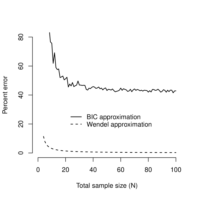
Figure 1: Average percent error of the BIC method and the Wendel method (each compared to analytic Pearson Bayes factor) for values of total sample size $N$ ranging from 4 to 100.

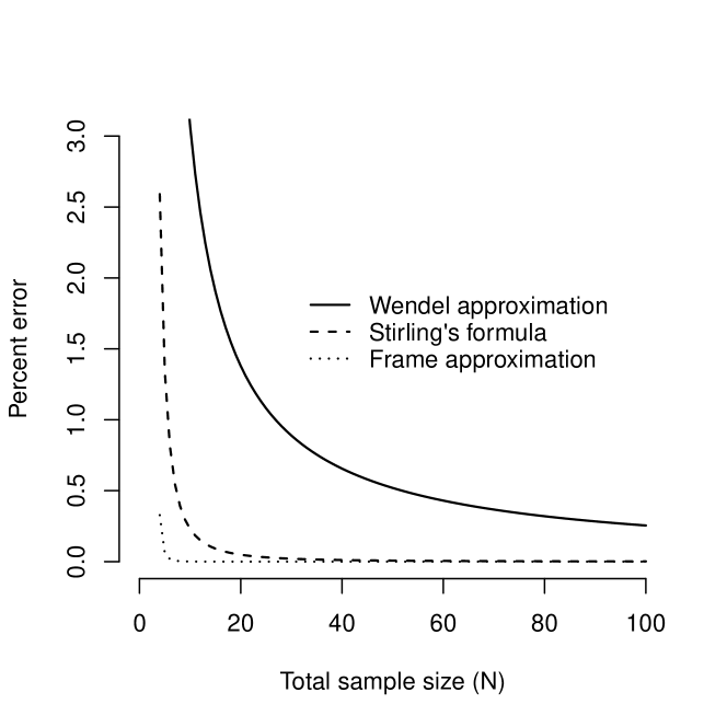
Figure 2: Average percent error of the Wendel, Stirling, and Frame methods (compared to analytic Bayes factor) for values of total sample size $N$ ranging from 4 to 100.

4 Conclusion

In this paper, I have presented three new closed-form approximations of the two-sample Pearson Bayes factor. These techniques allow the user to compute reasonably accurate approximations for Bayes factors in two-sample designs without the need for computing the Gamma function. As such, these computations may be performed using nothing more than a simple scientific calculator, making them a very attractive option for users who wish to compute Bayes factors directly from summary statistics in two-sample designs. Though the formulas vary in complexity, even the simplest formula based on Wendel’s (1948) asymptotic formula produces Bayes factor approximations with average percent error dropping below 1% for reasonably small sample sizes. As all three are asymptotic methods, their relative error will decrease with increasing sample sizes. This is a much better approach to approximating Bayes factors compared to the often-used BIC approximation (e.g., Kass and Raftery,, 1995; Wagenmakers,, 2007; Masson,, 2011; Faulkenberry,, 2018; Faulkenberry, 2020a, ; Faulkenberry,, 2019). The approximations presented here retain the spirit of the BIC Bayes factor (e.g., ease of use and ability to compute using only summary statistics), but as demonstrated, they provide a much better level of accuracy. Thus, these approximations are the ideal tool for easily computing evidential value in two-sample designs.

References

• Borota etΒ al., (2014) Borota, D., Murray, E., Keceli, G., Chang, A., Watabe, J.Β M., Ly, M., Toscano, J.Β P., and Yassa, M.Β A. (2014). Post-study caffeine administration enhances memory consolidation in humans. Nature Neuroscience, 17(2):201–203.
• Davis, (1959) Davis, P.Β J. (1959). Leonhard Euler’s integral: A historical profile of the Gamma function. American Mathematical Monthly, 66:849–869.
• (3) Faulkenberry, T. (2020a). Estimating bayes factors from minimal summary statistics in repeated measures analysis of variance designs. Advances in Methodology and Statistics, 17(1).
• Faulkenberry, (2018) Faulkenberry, T.Β J. (2018). Computing Bayes factors to measure evidence from experiments: An extension of the BIC approximation. Biometrical Letters, 55(1):31–43.
• Faulkenberry, (2019) Faulkenberry, T.Β J. (2019). Estimating evidential value from analysis of variance summaries: A comment on Ly (2018). Advances in Methods and Practices in Psychological Science, 2(4):406–409.
• (6) Faulkenberry, T.Β J. (2020b). The pearson bayes factor: An analytic formula for computing evidential value from minimal summary statistics.
• Faulkenberry and Brennan, (2023) Faulkenberry, T.Β J. and Brennan, K.Β B. (2023). Computing analytic bayes factors from summary statistics in repeated-measures designs. Biometrical Letters, 60(1):1–21.
• Frame, (1949) Frame, J.Β S. (1949). An approximation to the quotient of Gamma functions. American Mathematical Monthly, 56:529–535.
• Jameson, (2015) Jameson, G. J.Β O. (2015). A simple proof of Stirling’s formula for the gamma function. The Mathematical Gazette, 99:68–74.
• Kass and Raftery, (1995) Kass, R.Β E. and Raftery, A.Β E. (1995). Bayes factors. Journal of the American Statistical Association, 90(430):773.
• Masson, (2011) Masson, M. E.Β J. (2011). A tutorial on a practical Bayesian alternative to null-hypothesis significance testing. Behavior Research Methods, 43(3):679–690.
• Sellke etΒ al., (2001) Sellke, T., Bayarri, M.Β J., and Berger, J.Β O. (2001). Calibration of $p$-values for testing precise null hypotheses. The American Statistician, 55(1):62–71.
• Wagenmakers, (2007) Wagenmakers, E.-J. (2007). A practical solution to the pervasive problems of $p$ values. Psychonomic Bulletin & Review, 14(5):779–804.
• Wang and Liu, (2016) Wang, M. and Liu, G. (2016). A simple two-sample Bayesian $t$-test for hypothesis testing. The American Statistician, 70(2):195–201.
• Wendel, (1948) Wendel, J.Β G. (1948). Note on the Gamma function. American Mathematical Monthly, 55:563–564.