Elucidating The Design Space of Classifier-Guided Diffusion Generation

Abstract

Guidance in conditional diffusion generation is of great importance for sample quality and controllability. However, existing guidance schemes are to be desired. On one hand, mainstream methods such as classifier guidance and classifier-free guidance both require extra training with labeled data, which is time-consuming and unable to adapt to new conditions. On the other hand, training-free methods such as universal guidance, though more flexible, have yet to demonstrate comparable performance. In this work, through a comprehensive investigation into the design space, we show that it is possible to achieve significant performance improvements over existing guidance schemes by leveraging off-the-shelf classifiers in a training-free fashion, enjoying the best of both worlds. Employing calibration as a general guideline, we propose several pre-conditioning techniques to better exploit pretrained off-the-shelf classifiers for guiding diffusion generation. Extensive experiments on ImageNet validate our proposed method, showing that state-of-the-art diffusion models (DDPM, EDM, DiT) can be further improved (up to 20%) using off-the-shelf classifiers with barely any extra computational cost. With the proliferation of publicly available pretrained classifiers, our proposed approach has great potential and can be readily scaled up to text-to-image generation tasks. The code is available at https://github.com/AlexMaOLS/EluCD/tree/main.

1 Introduction

Diffusion probabilistic model (DPM) (Sohl-Dickstein et al., 2015; Ho et al., 2020; Song et al., 2020b) is a powerful generative model that employs a forward diffusion process to gradually add noise to data and generate new data from noise through a reversed process. DPM’s exceptional sample quality and scalability have significantly contributed to the success of Artificial Intelligence Generated Content (AIGC) in various domains, including images (Saharia et al., 2022; Ramesh et al., 2022, 2021; Rombach et al., 2022), videos (Ho et al., 2022b; Singer et al., 2022; Ho et al., 2022a; Molad et al., 2023), and 3D objects (Poole et al., 2022; Lin et al., 2023; Wang et al., 2023).

Conditional generation is one of the core tasks of AIGC. With the diffusion formulation, condition injection, especially the classical class condition, becomes more transparent as it can be modeled as an extra term during the reverse process. To align with the diffusion process, Dhariwal and Nichol (2021) proposed classifier guidance (CG) to train a time/noise-dependent classifier and demonstrated significant quality improvement over the unguided baseline. Ho and Salimans (2022) later proposed classifier-free guidance (CFG) to implicitly implement the classifier gradient with the score function difference and achieved superior performance in the classical class-conditional image generation. However, both CG and CFG require extra training with labeled data, which is not only time-consuming but also practically cumbersome, especially when adapting to new conditions. To reduce computational costs, training-free guidance methods have been proposed (Bansal et al., 2023) that take advantage of pretrained discriminative models. Despite the improved flexibility, training-free guidance has not demonstrated convincing performance compared to CG & CFG in formal quantitative evaluation of guiding diffusion generation. There seems to be an irreconcilable trade-off between performance and flexibility and the current guidance schemes are still to be desired.

In this work, we focus on the classical class-conditional diffusion generation setting and investigate the ideal method for guiding the diffusion generation, considering the following criteria: (1) Efficiency with training-free effort; (2) Superior performance in formal evaluation of guided conditional diffusion generation; and (3) Flexibility and adaptability to various new conditions. To this end, we delve into the properties of classifiers and rethink the design space of classifier guidance for diffusion generation. Through a comprehensive investigation both empirically and theoretically, we reveal that: (a) Trained/finetuned time-dependent classifiers have limitations; (b) Off-the-shelf classifiers’ potential is far from realized.

While existing methods primarily emphasize classifier accuracy, an ideal classifier should not only provide precise label predictions but also accurate estimations of the gradient of the logarithm of the conditional probability (Dhariwal and Nichol, 2021; Ho and Salimans, 2022; Chen et al., 2022). Given the challenges in efficiently estimating the gradient, classifier calibration emerges as a promising alternative, which quantifies how well a classifier recovers the ground truth conditional probability. We show that under certain smoothness conditions, a smaller calibration error leads to better estimation of the classifier gradient (Proposition 4.1). Accordingly, we propose the integral calibration error ($\overline{\text{ECE}}$) to assess classifier guidance along the diffusion reverse process and subsequently, effective pre-conditioning techniques to better prepare the classifier for guidance. Interestingly, our experiments reveal that trained/fine-tuned classifiers (Dhariwal and Nichol, 2021) are less calibrated than off-the-shelf ones when the noise level is high (Figure 1).

Beyond a good probability estimation, an ideal classifier guidance should also integrate seamlessly with the conditional diffusion generation process. Our investigation reveals that the naive implementation of classifier guidance will fade as the diffusion denoising step progresses, resulting in ineffective utilization of the classifier (Figure 4). To address this newly discovered issue, we propose a simple weighing strategy to balance the joint and conditional guidance, which significantly corrects the guidance direction and results in significantly improved sample quality.

To sum up, this work aims to elucidate the design space of classifier-guided diffusion generation. We carry out a comprehensive analysis of the classifier guidance, considering calibration, smoothness, guidance direction, and scheduling. Accordingly, we propose accessible and universal designs that significantly enhance guided sampling performance. Extensive experiments on ImageNet with various DPMs (DDPM, EDM, and DiT) validate our proposed method, showcasing that using off-the-shelf classifiers can consistently outperform both CG and CFG. Additionally, our method can be applied together with CFG and further enhance its generation quality. We also demonstrate the scalability and universality of our method in text-to-image scenarios by incorporating CLIP (Radford et al., 2021) guidance with our design. In comparison, we find that the operation of increasing recurrent guidance (Bansal et al., 2023) does not fully exploit the potential and comes at the expense of increasing sampling time.

2 Related Work

Diffusion models have gained considerable attention due to their capacity and potential. Ho et al. (2020); Nichol and Dhariwal (2021); Song et al. (2020a); Peebles and Xie (2022); Karras et al. (2022) demonstrated DPMs’ capacity in generating high-quality samples. Dhariwal and Nichol (2021) introduced fine-tuned time-dependent U-Net (Ronneberger et al., 2015) classifiers to guide diffusion model sampling, resulting in significant improvements. Ho and Salimans (2022) introduced classifier-free diffusion, which has been widely accepted (Rombach et al. (2022); Peebles and Xie (2022); Ramesh et al. (2022)) for generating high-quality samples using both conditional and unconditional diffusion models for inference. In our work, we demonstrate that our proposed off-the-shelf classifier-guided conditional diffusion not only significantly outperforms CG but also enhances the performance of CFG models (DiT Peebles and Xie (2022)). For guidance in other modalities, Nichol et al. (2021) proposed GLIDE, which utilizes fine-tuned noised CLIP for text-conditioned diffusion sampling. However, it requires the fine-tuning of CLIP on carefully selected noisy data.

In addition, research has explored using off-the-shelf checkpoints for diffusion sampling guidance. For example, Wallace et al. (2023) examined the plug-and-play of the classifier guidance, demanding the diffusion architecture to be invertible. Epstein et al. (2023) introduced self-guidance constraints for CLIP-guided sampling in objects’ editing. Bansal et al. (2023) applied recurrent guidance operation to universal pretrained models, but only provided demo figures without quantitative evaluation. However, our experiments in Table 1 reveal that increasing the recurrent guidance steps does not significantly improve the generation quality. In contrast, our calibrated off-the-shelf ResNet significantly enhances the sampling quality (lower Fréchet Inception Distance (FID) (Heusel et al., 2017)) without additional time, highlighting the effectiveness of our proposed guidance scheme.

Table 1: Evaluation of off-the-shelf ResNet with recurrent guidance operation and our calibrated designs in the guided sampling. The ResNet is the official Pytorch ResNet checkpoint; the diffusion model is from Dhariwal and Nichol (2021). We generate 10,000 ImageNet 128x128 samples with 250 DDPM steps for evaluation. Sampling time is recorded as GPU hours.

Classifier type	recurrent steps	FID	Time (hour)
ResNet	1	7.17	14.1
ResNet	2	7.06	16.0
ResNet	3	7.14	18.0
ResNet (Our-Calibrated)	1	5.19	14.1

3 Preliminaries

Diffusion model contains a series of time-dependent model components that apply the forward and reverse processes (Sohl-Dickstein et al., 2015; Ho et al., 2020). Forward process refers to the gradual increment of noise on the original sample $x_{0}$: $q(x_{t}|x_{0})=\mathcal{N}(x_{t};\sqrt{\bar{\alpha}_{t}}x_{0},(1-\bar{\alpha}_{t}))$ , where $\beta_{t}$ denotes forward process variance, $\alpha_{t}=1-\beta_{t},\bar{\alpha}_{t}=\Pi_{s=1}^{t}\alpha_{s}$. The reverse process refers to gradually generating clean samples from noisy samples: $p_{\theta}(\widehat{x}_{t-1}|\widehat{x}_{t})=\mathcal{N}(\widehat{x}_{t-1};\mu_{\theta}(\widehat{x}_{t},t),\sigma_{t})$, where $\mu_{\theta}(\widehat{x}_{t},t)$ is derived from removing the diffusion estimated $\epsilon_{\theta}(\widehat{x}_{t},t)$ from noisy samples $\widehat{x}_{t}$: $\mu_{\theta}(\widehat{x}_{t},t)=\frac{1}{\sqrt{\alpha_{t}}}(\widehat{x}_{t}-\frac{\beta_{t}}{\sqrt{1-\bar{\alpha}}_{t}}\epsilon_{\theta}(\widehat{x}_{t},t))$ and $\sigma_{t}$ denotes the reverse process variance.

Classifier guidance (Dhariwal and Nichol, 2021) can be applied in the reverse process for improving generation quality. For conditional diffusion classifier guidance and class $y$, the guided reverse process is adding $\mu_{\theta}$ with the gradient of the logarithm of the conditional probability: $\mathcal{N}(\widehat{x}_{t-1};\mu_{\theta}(\widehat{x}_{t},t)+s\sigma_{t}\nabla_{\widehat{x}_{t}}\log(p(y|\widehat{x}_{t})),\sigma_{t})$. Specifically, the gradient of the logarithm of classifier $f$ logit in softmax operation $\nabla_{\widehat{x}_{t}}\log(\text{softmax}(f_{y}(\widehat{x}_{t})))$ is used for $\nabla_{\widehat{x}_{t}}\log(p(y|\widehat{x}_{t}))$.

Classifier-free guidance (Ho and Salimans, 2022) uses the difference between conditional and unconditional noise (score) to represent the conditional probability guidance during the sampling, $\nabla_{\widehat{x}_{t}}\log(p(y|\widehat{x}_{t}))\propto\epsilon_{\theta}(\widehat{x}_{t},y,t)-\epsilon_{\theta}(\widehat{x}_{t},\emptyset,t)$. The classifier-free guided sampling becomes $\epsilon_{t}^{*}=\epsilon_{\theta}(\widehat{x}_{t},y,t)+(s-1)(\epsilon_{\theta}(\widehat{x}_{t},y,t)-\epsilon_{\theta}(\widehat{x}_{t},\emptyset,t))$, where $s>1$ is the classifier-free scale. The unconditional $\epsilon_{\theta}(\widehat{x}_{t},\emptyset,t)$ is trained by randomly replacing the class with null class $\emptyset$.

4 Design Space of Classifier Guidance

4.1 Classifiers: Fine-tuned vs Off-the-Shelf

According to Dhariwal and Nichol (2021), a classifier to be used for guiding diffusion generation requires dedicated training or fine-tuning to adapt to noisy images at different time steps during the diffusion process. To implement the time-dependency, the classifier usually employs the downsampling component of U-Net (Ronneberger et al., 2015), and fine-tuning is performed on noisy samples $x_{t}$ for every $t$ along the forward diffusion process. Such a training procedure is time-consuming (200+ GPU hours for ImageNet 128x128), which greatly limits its efficiency.

In comparison, “off-the-shelf” classifiers refer to the publicly available checkpoints that can be directly deployed without any further fine-tuning. The collection of such pretrained classifiers is becoming increasingly more powerful and diverse. There is a line of research, under the umbrella of “model zoo”, that specifically studies how to explore and exploit pretrained models for various downstream tasks (Shu et al., 2021; Dong et al., 2022; Chen et al., 2023; Luo et al., 2023). However, when it comes to guiding diffusion generation, “off-the-shelf” classifiers tend to be not robust against Gaussian noise and not adaptable to time-dependent diffusion architectures. Successfully exploiting their knowledge for diffusion models is non-trivial and requires careful designs. In our work, we use the official Pytorch ResNet checkpoints as the off-the-shelf classifiers.

As stated earlier, while an ideal classifier for guiding diffusion should provide accurate estimations of $\nabla\log P(y|x)$, calibration error is a promising alternative criterion due to the challenges in efficient gradient estimation. Proposition 4.1 suggests that if a classifier satisfies certain smoothness conditions, a small calibration error indicates a good estimation of the gradient of the log conditional probability, which will, in turn, provide better guidance to diffusion generation.

Proposition 4.1.

Let $p\in\mathcal{H}^{k}(\Omega)$ be the underlying true density function, where $\mathcal{H}^{k}(\Omega)$ is the Sobolev space with smoothness $k>1$ defined on a compact and convex region $\Omega$. Assume that there exist constants $c_{1},c_{2}>0$ such that $c_{2}\geq p(\bm{x})\geq c_{1},\forall\bm{x}\in\Omega$. Suppose $p_{n}$ is an estimate of $p$ such that $\|p_{n}\|_{\mathcal{H}^{k}(\Omega)}\leq C$ for some constant $C$ not depending on $n$, where $n$ is the sample size. If $\|p_{n}-p\|_{L_{2}(\Omega)}=o_{\mathbb{P}}(1)$, we have $\|\nabla\log p-\nabla\log p_{n}\|_{L_{2}(\Omega)}=o_{\mathbb{P}}(1)$.

To quantitatively assess the calibration of a classifier and its compatibility with the diffusion model, we propose the integral calibration error $\overline{\text{ECE}}$ (Eq.1) as an estimation of $\int_{t}\text{ECE}_{t}$, where $\text{ECE}_{t}$ (Expected Calibration Error (Naeini et al., 2015)) measures the sample average of the difference between the classifier’s accuracy and probability confidence within bins $B$ based on the reverse process sample $\widehat{x}_{t}$ at time $t$.

$$\overline{\text{ECE}}=\frac{1}{k}\sum_{t=0}^{k}\text{ECE}_{t},\text{ where }\text{ECE}_{t}=\sum^{M}_{m=1}\frac{|B_{m}|}{n}|\text{acc}(B_{m}(\widehat{x}_{t}))-\text{conf}(B_{m}(\widehat{x}_{t}))|.\\$$ (1)

Figure 1 depicts the $\text{ECE}_{t}$ curves of the two classifiers at different time stages (250 DDPM steps in total). From time 0 to 50, the fine-tuned classifier exhibits lower $\text{ECE}_{t}$ values compared to ResNet, demonstrating its robustness to Gaussian noise when the images are less noisy. However, as the time steps progress and the noise magnitude increases, the off-the-shelf ResNet achieves lower $\text{ECE}_{t}$ values than the fine-tuned classifier. This suggests that training on highly noisy or low signal-to-noise samples does not contribute to the fine-tuned classifier guidance. This observation forms the basis that off-the-shelf guidance has the potential to not only match but also surpass the performance of fine-tuned classifiers in our experiments.

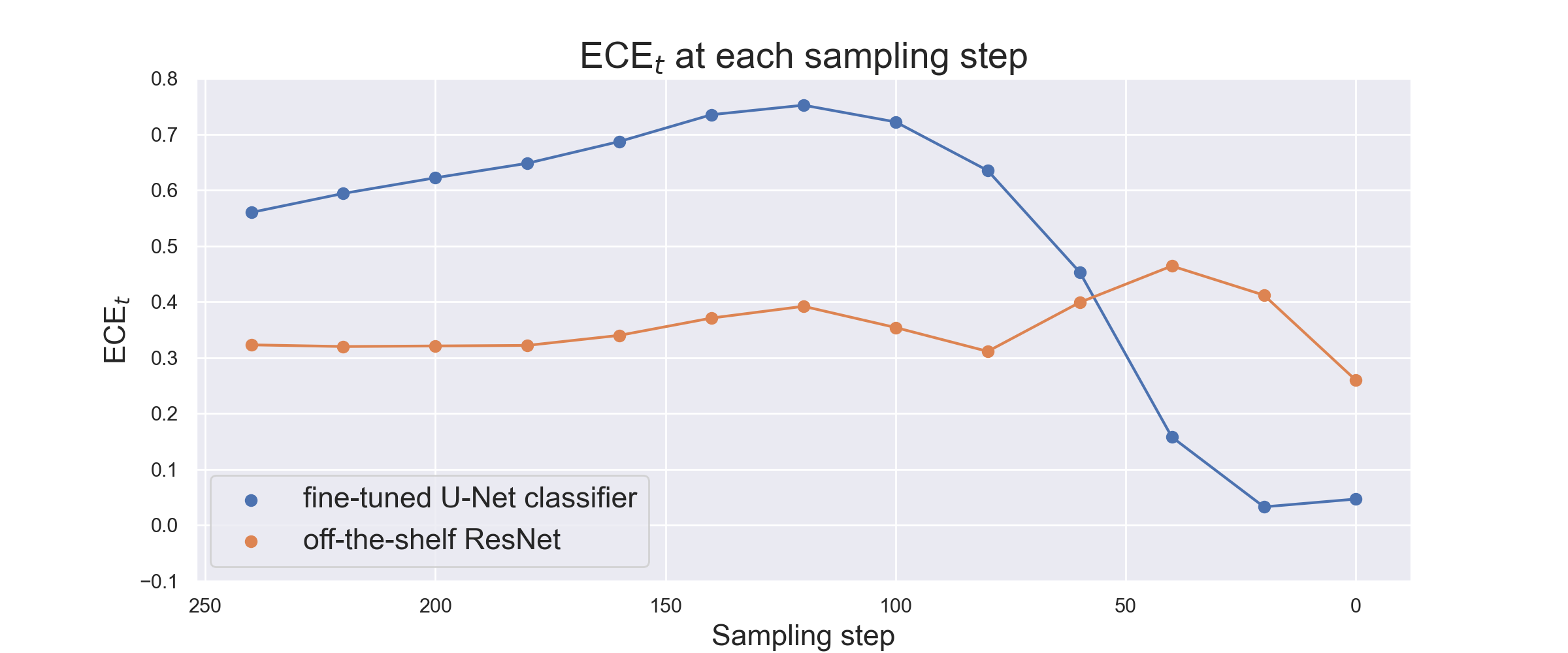
Figure 1: The $\text{ECE}_{t}$ of the fine-tuned and the off-the-shelf classifiers throughout sampling step.

To further verify the connection between integral calibration error and diffusion guidance quality, we conduct experiments in guided image generation using different classifiers and evaluate the FID. Besides the fine-tuned and off-the-shelf classifiers, we also consider the “combined" classifier, i.e., off-the-shelf ResNet in time 250 to 50 and the fine-tuned classifier in time 50 to 0, which is more calibrated. The results are shown in Table 2, where we can clearly see that the FID is positively correlated with $\overline{\text{ECE}}$. It validates that the accurate estimation of probability (lower ECE) contributes to better generation quality.

Table 2: Comparative analysis of different classifier choices in guided sampling. The fine-tuned classifier is from Dhariwal and Nichol (2021) and the ResNet is the official Pytorch ResNet checkpoint; the diffusion model is from Dhariwal and Nichol (2021) and the dataset is ImageNet 128x128. Generating 10000 samples with 250 DDPM steps for evaluation.

Classifier type	$\overline{\text{ECE}}$	FID
fine-tuned	0.51	8.27
ResNet	0.35	7.17
ResNet & fine-tuned	0.28	6.94

In the subsequent sections, we explore the design space of classifier-guided diffusion generation with the aim of enhancing the quality of the classifier gradients along the diffusion process and having better synergy with the diffusion score function. Accordingly, we propose the following designs:

• Classifier inputs: to facilitate calibration with the diffusion reverse process, we provide the off-the-shelf classifier with the predicted denoised sample $\widehat{x}_{0}(t)$ during reverse sampling.

• Smooth guidance: building on Proposition 4.1, we enhance the smoothness of the classifier, enabling calibration to result in improved guidance (gradient estimation).

• Guidance direction: we uncover the classifier guidance diminishes as the diffusion denoising step advances in Figure 4. To address this, we balance the joint and conditional guidance direction and result in optimal guidance direction.

• Guidance schedule: we propose a simple yet effective Sine guidance schedule that better aligns with the calibration error curve (Figure 1) of the off-the-shelf classifier.

4.2 Predicted Denoised Samples

During the classifier-guided reverse diffusion sampling process, there are two types of intermediate sample to be used for the classifier: the reverse-process sample $\widehat{x}_{t}$, and the predicted denoised sample: $\widehat{x}_{0}(t)=(\widehat{x}_{t}-(\sqrt{1-\alpha_{t}})\epsilon_{\theta}(\widehat{x}_{t},t))/\sqrt{\alpha_{t}}$ (Song et al. (2020a); Bansal et al. (2023)). Considering off-the-shelf classifiers are typically not robust to Gaussian noise and not time-dependent, selecting the appropriate classifier input type is crucial to ensure the best fit. In Table 3, we compare the calibration of two input types: the reverse-process samples $\widehat{x}_{t}$ and the predicted denoised samples $\widehat{x}_{0}(t)$ used in the guided diffusion. Table 3 demonstrates that the off-the-shelf ResNet classifier achieves better calibration when provided with the denoised sample $\widehat{x}_{0}(t)$ compared to $\widehat{x}_{t}$. This improvement in calibration enhances the guided sampling quality with a smaller FID.

Table 3: Comparison of classifier inputs in guided sampling with respect to $\overline{\text{ECE}}$ and FID. Denote the guidance of classifier $f$ as $\text{Guidance}(x):=\nabla_{x}\log(\text{softmax}(f_{y}(x)))$. The classifier is the official Pytorch ResNet checkpoint; the diffusion model is from Dhariwal and Nichol (2021). We generate 10,000 ImageNet 128x128 samples with 250 DDPM steps for evaluation.

	$\text{guidance}(\widehat{x}_{t})$	$\text{guidance}(\widehat{x}_{0}(t))$
$\overline{\text{ECE}}$	0.36	0.28
FID	8.61	7.17

4.3 Smooth Classifier

A smooth classifier is important to the success of guided diffusion generation. On one hand, Proposition 4.1 indicates that the smoothness of the classifier is key to ensuring good gradient estimation. On the other hand, gradient-based optimization also benefits from increased smoothness. For better guidance, we propose to enhance the smoothness of the off-the-shelf classifier. According to Zhu et al. (2021), the following Softplus activation function (Nair and Hinton, 2010) is effective in smoothing the classifier gradient.

$$\text{Softplus}_{\beta}(x)=\frac{1}{\beta}\log(1+\exp(\beta x)).$$

As parameter $\beta$ approaches infinity, the Softplus function converges to the ReLU activation function. Table 4 and Figure 2 demonstrate that as $\beta$ decreases, the $\overline{\text{ECE}}$ decreases as well, indicating that smoother activation benefits classifier calibration. Consequently, the well-calibrated design enhances the guided sampling performance compared to the baseline (ReLU), reducing FID from 7.17 to 6.61.

Table 4: Ablation study of $\beta$ in Softplus with respect to integral calibration error $\overline{\text{ECE}}$ and FID. The classifier is the official Pytorch ResNet checkpoint. The diffusion model is from Dhariwal and Nichol (2021). We generate 10,000 ImageNet 128x128 samples with 250 DDPM steps for evaluation.

	ReLU	SoftPlus ($\beta$=8)	SoftPlus ($\beta$=5)	SoftPlus ($\beta$=4)	SoftPlus ($\beta$=3)
$\overline{\text{ECE}}$	0.34	0.31	0.26	0.21	0.07
FID	7.17	6.99	6.89	6.73	6.61

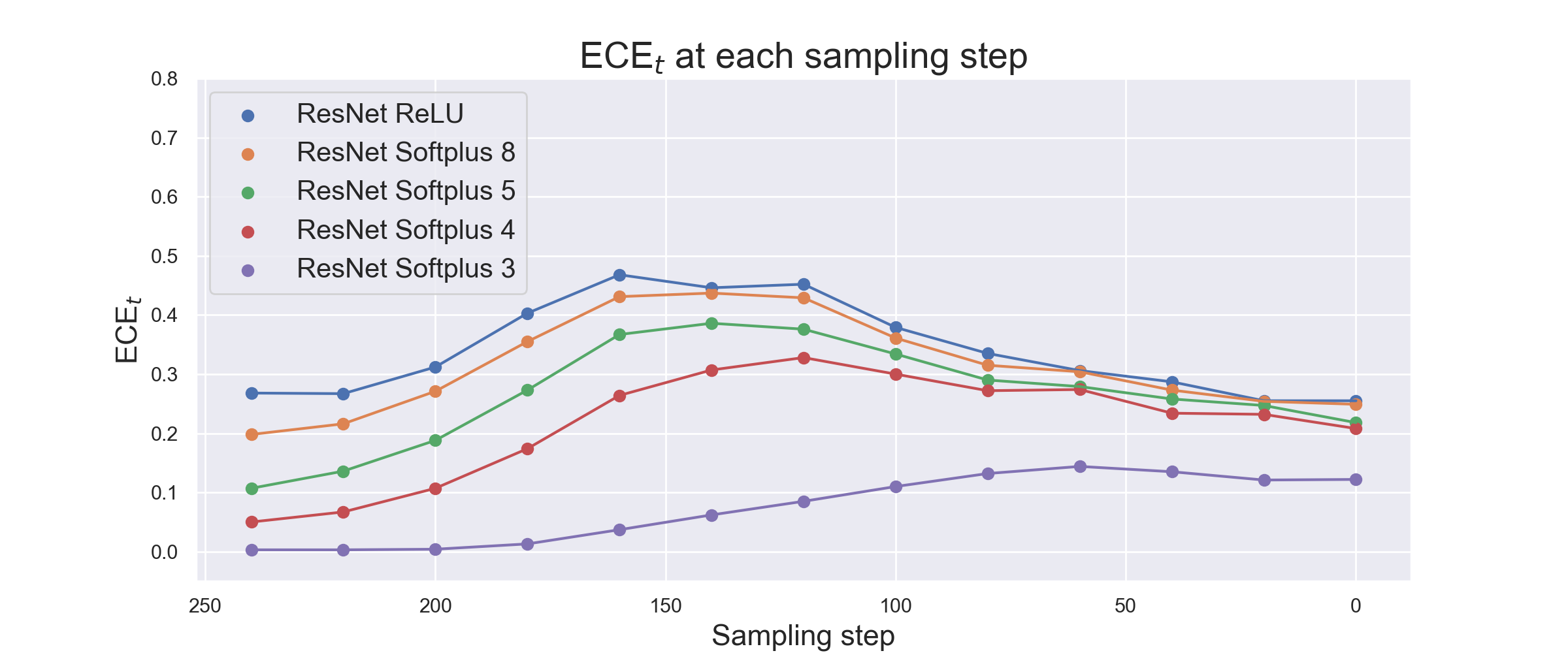
Figure 2: The $\text{ECE}_{t}$ curves of the off-the-shelf ResNet with ReLU and Softplus activation functions.

4.4 Joint vs Conditional Direction

In Dhariwal and Nichol (2021), the classifier guidance is defined as the gradient of the conditional probability, which can be interpreted as the gradient of the joint and marginal energy (Grathwohl et al., 2019) difference, shown in Eq.(2) and (3) as

$$\log p_{\tau}(y|x)=\log\frac{\exp(\tau f_{y}(x))}{\sum^{N}_{i=1}\exp(\tau f_{i}(x))} =\tau f_{y}(x)-\log{\sum^{N}_{i=1}\exp(\tau f_{i}(x))}:=-E_{\tau}(x,y)+E_{\tau}(x),$$ (2)

$$\nabla_{x}\log p_{\tau}(y|x)=-\nabla_{x}E_{\tau}(x,y)+\nabla_{x}E_{\tau}(x)$$ (3)

In this section, we demonstrate that properly weighing the joint and conditional guidance can significantly improve sampling quality.

To gain a deeper understanding of the guidance direction, we conduct a closed-form analysis in mixed-Gaussian scenarios. Proposition 4.2 provides the derived closed-form joint and conditional directions in mixed-Gaussian scenarios: for conditional probability gradient, the guidance direction is a combination of class mode differences, while the joint probability gradient directly targets the objective class mode $\mu_{l}$. Figure 3 provides a visual illustration.

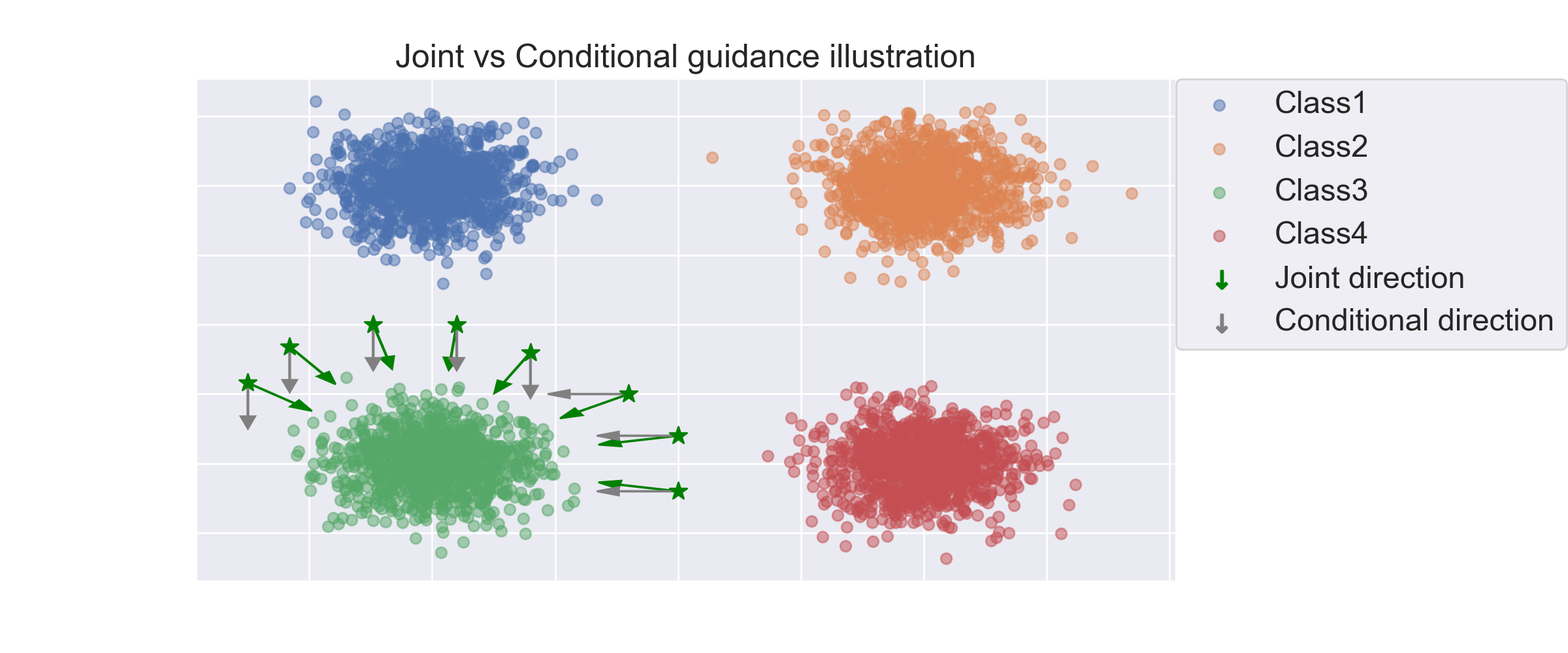
Figure 3: Mixed-Gaussian settings of joint and conditional probability guidance toward Class3.

Proposition 4.2.

Let $X\sim P$ be a random variable defined on $\mathbb{R}^{d}$, with the density function $f(\bm{x})=\sum_{k=1}^{K}b_{k}f_{k}(\bm{x})$, where $f_{k}(\bm{x})$ is a normal density function with mean $\bm{\mu}_{k}$ and covariance matrix $\bm{\Sigma}_{k}$, and $b_{k}>0$ with $\sum_{k=1}^{K}b_{k}=1$. Let $Z\in\{1,...,K\}$ be a random variable satisfying $P(Z=l,X=\bm{x})=b_{l}f_{l}(\bm{x})$. Then we have

$$\nabla_{\bm{x}}P(Z=l|X=\bm{x})\propto \sum_{k=1}^{K}b_{k}e^{-\frac{1}{2}(\bm{x}-\bm{\mu}_{k})^{\top}\bm{\Sigma}_{k}^{-1}(\bm{x}-\bm{\mu}_{k})}(\bm{\Sigma}_{l}^{-1}(\bm{x}-\bm{\mu}_{l})-\bm{\Sigma}_{k}^{-1}(\bm{x}-\bm{\mu}_{k})),$$

$$\nabla_{\bm{x}}P(Z=l,X=\bm{x})\propto \bm{\Sigma}_{l}^{-1}(\bm{\mu}_{l}-\bm{x}).$$

Proposition 4.2 reveals that if all $\bm{\Sigma}_{k}$ are identity matrices, the gradient of the joint distribution is simply $\bm{\mu}_{l}-\bm{x}$, directing towards the mode of density $f_{l}(\bm{x})$, while the gradient of the conditional distribution is $\sum_{k=1}^{K}b_{k}e^{-\frac{1}{2}(\bm{x}-\bm{\mu}_{k})^{\top}(\bm{x}-\bm{\mu}_{k})}(\bm{\mu}_{k}-\bm{\mu}_{l})$, which may point to low-density region. This behavior is illustrated in Figure 3.

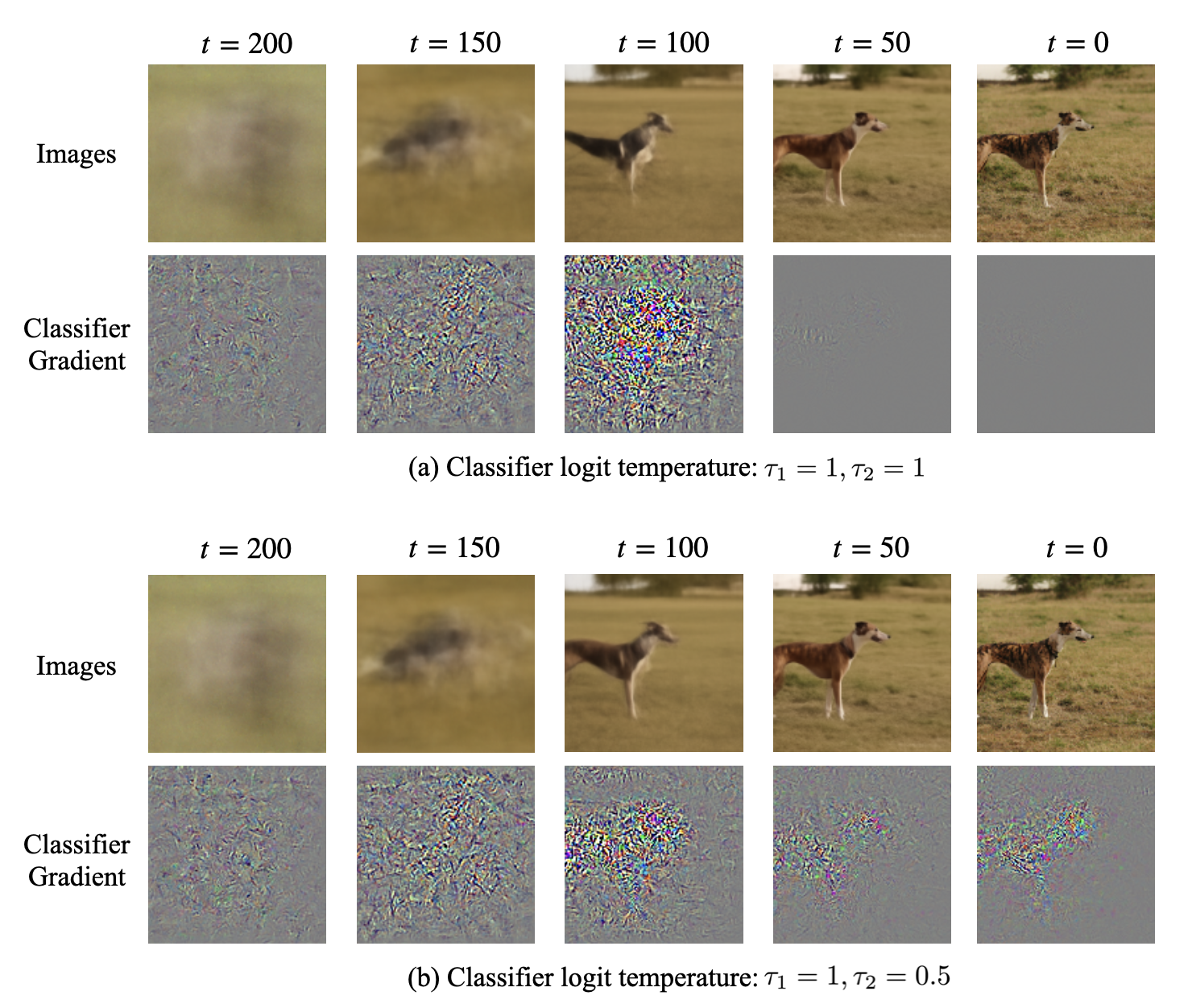
Figure 4: The visualization of intermediate sampling images and classifier gradient figures under conditional probability and joint-strengthened guidance over 250 DDPM steps.

To strengthen the joint $f_{y}(x)$ guidance (joint energy $E_{\tau_{1}}(x,y)$), we reduce the value of marginal temperature $\tau_{2}$ relative to the joint temperature $\tau_{1}$, as shown in Eq.(4). The ablation study in Table 5 validates the improvement in the sampling quality by weighing the joint & marginal guidance.

$$\nabla_{x}\log p_{\tau_{1},\tau_{2}}(y|x) =\nabla_{x}(\tau_{1}f_{y}(x)-\log(\sum^{N}_{i=1}\exp(\tau_{2}f_{i}(x)))):=-\nabla_{x}E_{\tau_{1}}(x,y)+\nabla_{x}E_{\tau_{2}}(x)$$ (4)

Table 5: Ablation study of marginal logit temperature $\tau_{2}$ with respect to FID. $\tau_{1}$ is fixed as 1.

$\tau_{2}$	1.0	0.8	0.7	0.5	0.3
FID	6.20	5.62	5.45	5.27	5.30

In addition to quantitative metrics, we visually demonstrate the impact of enhancing joint guidance on classifier-guided sampling. Figure 4 displays the intermediate sampling images and the classifier gradient figures over 250 DDPM steps. Figure 4 (a) represents the traditional conditional probability settings ($\tau_{1}=1,\tau_{2}=1$): the classifier gradient figure gradually fades from $t=50$ to 0, indicating a loss of dog depiction guidance during the sampling. In contrast, Figure 4 (b) showcases strengthened joint guidance ($\tau_{1}=1,\tau_{2}=0.5$): the classifier gradient figure increasingly highlights the dog’s outline, providing consistent and accurate guidance direction throughout the entire sampling process. This observation aligns with Proposition 4.2, highlighting that the gradient of the conditional distribution may point to a low-density region, while the jointly amplified gradient targets the mode of density more precisely.

4.5 Guidance Schedule

In Dhariwal and Nichol (2021), the classifier guidance scale schedule employs a linear timely-decay variance $\sigma_{t}=\beta_{t}$ (Ho et al., 2020). To fully leverage the benefits of a well-calibrated classifier, we introduce an extra $\sin$ component to the guidance schedule:

$$\gamma_{t}=\sigma_{t}+\gamma\sigma_{T}\cdot\sin(\pi t/T),$$ (5)

where $\sigma_{t}$ denotes the variance at time $t$. This design choice is motivated by the observation in Figure 1, where the off-the-shelf classifier exhibits consistently lower and more stable $\text{ECE}_{t}$ values during the large noise period (from the beginning to the middle of the reverse process). Consequently, we can amplify the guidance scale during this period to better exploit its effectiveness. The parameter $\gamma$ is used for controlling the magnitude of the guidance amplifying: the bigger the parameter $\gamma$, the greater the time-dependent $\sin$ value added to the guidance schedule. Figure 5 demonstrates the original schedule and the updated schedule with sine factor $\gamma$ added. The impact of the added factor $\gamma$ is examined in the ablation study presented in Table 6. The effectiveness of our proposed guidance schedule is also demonstrated in the case of CLIP-guided text-to-image generation. Please refer to Figure 7 in Section 5.4.

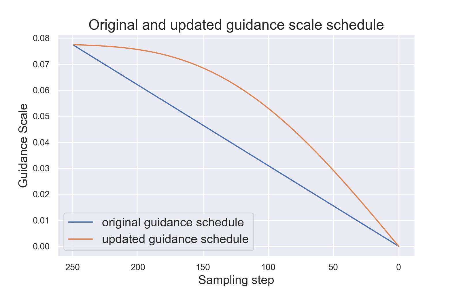
Figure 5: The comparison of linear guidance schedule and updated guidance schedule with sine factor $\gamma=0.3$ in (5).

Table 6: Ablation study of sine factor $\gamma$ on classifier guidance with respect to FID. The classifier is the official Pytorch ResNet checkpoint; the diffusion model is from Dhariwal and Nichol (2021). We generate 10,000 ImageNet 128x128 samples with 250 DDPM steps for evaluation.

$\gamma$	0.0	0.1	0.2	0.3	0.4
FID	5.57	5.30	5.27	5.24	5.38

5 Experiments

5.1 Off-the-Shelf Guidance for DDPM

Guided diffusion (Dhariwal and Nichol, 2021) demonstrates that incorporating a fine-tuned U-Net classifier can significantly enhance image generation quality. However, the classifier is demanded to be a time-dependent U-Net, and the fine-tuning process is time-consuming (200+ GPU hours for ImageNet128x128 classifier fine-tuning). In our approach, we utilize off-the-shelf PyTorch ResNet-50 and ResNet-101 checkpoints with our calibrated design to directly guide the diffusion sampling. Table 7 confirms that our calibrated off-the-shelf ResNet-50 (FID: 2.36) and ResNet-101 (FID: 2.19) not only improve the diffusion baseline quality (FID: 5.91) but also outperforms the fine-tuned classifier guided diffusion (FID: 2.97) and the classifier-free diffusion (Ho and Salimans, 2022) (FID: 2.43) by a significant margin. By leveraging off-the-shelf classifiers, we integrate external knowledge into conditional diffusion models, surpassing existing approaches. The guided sampling algorithm is outlined in Algorithm 1 and the hyper-parameter settings can be found in Appendix C.1.

Table 7: The comparison of the baseline DDPM diffusion, the fine-tuned classifier-guided, classifier-free diffusion, and the off-the-shelf ResNet guided sampling. All models are sampled for 250 DDPM steps. We generate 50,000 ImageNet 128x128 samples for evaluation.

ImageNet 128x128	Classifier	FID
Diffusion baseline (Dhariwal and Nichol (2021))	-	5.91
Diffusion Finetune guided (Dhariwal and Nichol (2021))	Fine-tune	2.97
Classifier-free Diffusion (Ho and Salimans (2022))	-	2.43
Diffusion ResNet50 guided (ours)	Off-the-Shelf	2.36
Diffusion ResNet101 guided (ours)	Off-the-Shelf	2.19

Algorithm 1 DDPM off-the-shelf classifier guided sampling.

Parameter: SoftPlus activation $\beta$, joint logit temperature $\tau_{1}$, marginal logit temperature $\tau_{2}$. classifier guidance scale $\gamma_{t}$.

Required: Diffusion model $D_{\theta}$, variance schedule $\sigma_{t}$, class label $y$, reverse process sample $\widehat{x}_{t}$, predicted denoised sample $\widehat{x}_{0}(t)$, reverse process noise $\epsilon_{\theta}(\widehat{x}_{t},y,t)$, classifier logit of input $x$ on class $y$: $f_{y}(x)$.

$\widehat{x}_{T}$ sampled from $\mathcal{N}(0,\mathbb{I})$

for $t\in$ $\{T,...,1\}$ do

     $\mu,\epsilon_{\theta}(\widehat{x}_{t},y,t)\leftarrow D_{\theta}(\widehat{x}_{t},y,t)$

     $\widehat{x}_{0}(t)\leftarrow(\widehat{x}_{t}-(\sqrt{1-\alpha_{t}}\epsilon_{\theta}(\widehat{x}_{t},y,t)))/\sqrt{\alpha_{t}}$ $\triangleright$ get predicted denoised sample

     $g\leftarrow\nabla_{\widehat{x}_{0}(t)}\log(\exp(\tau_{1}f_{y}(\widehat{x}_{0}(t)))/(\sum^{N}_{i=1}\exp(\tau_{2}f_{i}(\widehat{x}_{0}(t)))))$ $\triangleright$ classifier gradient guidance

     $\widehat{x}_{t-1}\leftarrow\text{sample from }\mathcal{N}(\mu+\gamma_{t}g,\sigma_{t})$

end for

return $\widehat{x}_{0}$

5.2 Off-the-Shelf Guidance for EDM

In this section, we demonstrate the effectiveness of off-the-shelf classifier guidance in fewer sampling steps based on the EDM model (Karras et al., 2022). EDM utilizes a sampling trajectory based on the sampling curvature $d_{t}=dx/dt$, enabling efficient and high-quality image generation. Our EDM guided-sampling algorithm is outlined in Algorithm 2, where the normalized sample $\widehat{x}_{i}/\lVert\widehat{x}_{i}\rVert_{2}$ is used as the classifier guidance inputs, i.e., $g=\nabla\log(\text{softmax}f(\widehat{x}_{i}/\lVert\widehat{x}_{i}\rVert_{2}))$. Then the gradient $g$ is normalized to align with the sample $\widehat{x}_{i}$ and curvature $d_{i}$:

$$\widehat{x}_{i-1}\leftarrow\widehat{x}_{i}+(t_{i}-t_{i-1})d_{i}+\gamma_{i}(g/\lVert g\rVert_{2}).$$

In our experiments, we present the results of off-the-shelf classifier guidance results of ODE sampling on ImageNet 64x64 in Table 8, with the sampling time recorded as GPU hours. The results of 250 steps of SDE sampling (Kingma and Gao, 2023) can be found in Table C.1 of Appendix C.2.

Algorithm 2 EDM off-the-shelf classifier guided sampling.

Parameter: SoftPlus activation $\beta$, joint logit temperature $\tau_{1}$, marginal logit temperature $\tau_{2}$. classifier guidance scale $\gamma_{i}$.

Required: EDM model $E_{\theta}$, class label $y$, reverse process sample $\widehat{x}_{i}$, curvate $d_{i}$, classifier logit of input $x$ on class $y$: $f_{y}(x)$.

$\widehat{x}_{N}$ sample from $\mathcal{N}(0,\mathbb{I})$

for $i\in$ $\{N,...,1\}$ do

     $d_{i},t_{i}\leftarrow E_{\theta}(\widehat{x}_{i})$

     $\bar{x}_{i}\leftarrow\widehat{x}_{i}/\lVert\widehat{x}_{i}\rVert_{2}$ $\triangleright$ sample $\widehat{x}_{i}$ normalization

     $g\leftarrow\nabla_{\bar{x}_{i}}\log(\exp(f_{y}(\bar{x}_{i})\tau_{1})/(\sum^{N}_{k=1}\exp(f_{k}(\bar{x}_{i})\tau_{2})))$

     $\widehat{x}_{i-1}\leftarrow\widehat{x}_{i}+(t_{i}-t_{i-1})d_{i}+\gamma_{i}(g/\lVert g\rVert_{2})$ $\triangleright$ normalized classifier gradient as guidance

     if $t_{i-1}\neq 0$ then

         $\widehat{x}_{i-1}\leftarrow E_{\theta}(\widehat{x}_{i},\widehat{x}_{i-1},t_{i},t_{i-1})$

     end if

end for

return $\widehat{x}_{0}$

Table 8: EDM (Karras et al., 2022) baseline and the off-the-shelf ResNet guided EDM sampling. Sampled for multiple ODE steps. We generate 50,000 ImageNet 64x64 samples for evaluation.

ImageNet 64x64	Classifier	FID	Steps	Time(hour)
EDM baseline	-	2.35	36	8.0
EDM Res101 guided	Off-the-Shelf	2.22	36	8.4
EDM baseline	-	2.54	18	4.0
EDM Res101 guided	Off-the-Shelf	2.35	18	4.1
EDM baseline	-	3.64	10	2.1
EDM Res101 guided	Off-the-Shelf	3.38	10	2.2

5.3 Off-the-Shelf Guidance for DiT

In order to reduce the computation cost, many successful generative models leverage a low-dimensional latent space (Chang et al., 2022; Vahdat et al., 2021; Hu et al., 2023), e.g., Stable Diffusion (Rombach et al., 2022) models the latent space induced by an encoder and generates images through a paired decoder. Successful adaptation of our method to such latent diffusion models is appealing. In this section, we showcase the applicability of off-the-shelf guidance in enhancing latent-spaced classifier-free diffusion models, specifically Diffusion Transformers (DiT) (Peebles and Xie, 2022), which stands out in several aspects. Firstly, it utilizes transformer architecture instead of U-Net. Secondly, DiT operates in the latent space, which is encoded by a variational autoencoder (VAE) (Kingma and Welling, 2013) from Stable Diffusion (Rombach et al., 2022). Lastly, DiT is trained in classifier-free setup (Ho and Salimans, 2022). Our DiT guided-sampling algorithm is outlined in Algorithm 3, and the guided performance is presented in Table 9. Unlike Wallace et al. (2023), our off-the-shelf classifier guidance does not require retraining a latent-space-based classifier and imposes no requirements on the diffusion architectures. Notably, there are two featuring designs in the Algorithm 3:

1. To integrate the pixel-spaced classifier $f$ into latent sampling, we consider the guidance $g$ as the gradient of composite functions, specifically the VAE decoder $V_{D}$ within the classifier $f$. It can be expressed as: $g=\nabla_{\widehat{z}_{0}(t)}\log(\text{softmax}f(V_{D}(\widehat{z}_{0}(t))))$.

2. To incorporate classifier guidance $g$ into classifier-free sampling, we normalize the guidance and add the normalized $\bar{g}$ to the conditional and unconditional noise difference. The formula is as follows:

   $$\epsilon_{\theta}(\widehat{z}_{t},c,t)+(s-1)(\epsilon_{\theta}(\widehat{z}_{t},c,t)-\epsilon_{\theta}(\widehat{z}_{t},\emptyset,t)+\gamma_{t}\bar{g}).$$

Algorithm 3 Off-the-shelf classifier guidance for DiT sampling.

Parameter: classifier-free scale $s$, classifier guidance scale $\gamma_{t}$, joint logit temperature $\tau_{1}$, marginal logit temperature $\tau_{2}$.

Required: DiT model $D_{\theta}$, VAE decoder $V_{D}$, classifier logit of input $x$ on class $y$: $f_{y}(x)$, class label $y$, reverse process class-conditional and unconditional noise $\epsilon_{\theta}(\widehat{z}_{t},c,t)$ and $\epsilon_{\theta}(\widehat{z}_{t},\emptyset,t)$, reverse process latent and pixel spaced sample $\widehat{z}_{t}$ and $\widehat{x}_{t}$, predicted denoised latent and pixel spaced sample $\widehat{z}_{0}(t)$ and $\widehat{x}_{0}(t)$.

$\widehat{z}_{T}$ sample from $\mathcal{N}(0,\mathbb{I})$

for $t\in$ $\{T-1,...,0\}$ do

     $\widehat{z}_{0}(t),\epsilon_{\theta}(\widehat{z}_{t},c,t),\epsilon_{\theta}(\widehat{z}_{t},\emptyset,t)\leftarrow D_{\theta}(\widehat{z}_{t},t)$

     $\widehat{x}_{0}(t)\leftarrow V_{D}(\widehat{z}_{0}(t))$ $\triangleright$ VAE decoder transform latent sample into pixel space

     $g\leftarrow\nabla_{\widehat{z}_{0}(t)}\log(\exp(f_{y}(\widehat{x}_{0}(t))\tau_{1})/(\sum^{N}_{i=1}\exp(f_{i}(\widehat{x}_{0}(t))\tau_{2})))$ $\triangleright$ classifier gradient guidance

     $\Delta\epsilon_{t}\leftarrow\epsilon_{\theta}(\widehat{z}_{t},c,t)-\epsilon_{\theta}(\widehat{z}_{t},\emptyset,t)$

     $\bar{g}\leftarrow(g/\lVert g\rVert_{2})\lVert\Delta\epsilon_{t}\rVert_{2}$ $\triangleright$ classifier guidance normalization

     $\epsilon_{t}^{*}\leftarrow\epsilon_{\theta}(\widehat{z}_{t},c,t)+(s-1)(\Delta\epsilon_{t}+\gamma_{t}\bar{g})$ $\triangleright$ classifier guidance into classifier-free

     $\mu\leftarrow\frac{1}{\sqrt{\alpha_{t}}}(\widehat{z}_{t}-\frac{\beta_{t}}{\sqrt{1-\bar{\alpha}_{t}}}\epsilon_{t}^{*})$ $\triangleright$ posterior mean Ho et al. (2020)

     $\widehat{z}_{t-1}\leftarrow\text{sample from }\mathcal{N}(\mu,\sigma_{t})$

end for

$\widehat{x}_{0}\leftarrow V_{D}(\widehat{z}_{0})$

return $\widehat{x}_{0}$

Table 9: DiT (Peebles and Xie, 2022) baseline and the off-the-shelf ResNet guided DiT sampling, sampled for 250 DDPM steps. We generate 50,000 ImageNet 256x256 samples for evaluation.

ImageNet 256x256	Classifier	FID	Precision	Recall
DiT baseline	-	2.27	0.828	0.57
DiT ResNet101 guided	Off-the-Shelf	2.12	0.817	0.59

5.4 CLIP-guided Diffusion

In this section, we utilize off-the-shelf CLIP (Radford et al., 2021) to guide the conditional diffusion model (Dhariwal and Nichol, 2021) in generating images based on a given prompt (see Eq.D.1 in Appendix D). Compared to approaches in Bansal et al. (2023); Wallace et al. (2023), our text-to-image sampling method achieves more efficient and high-quality samples. Our method does not require recurrent guidance iteration within a single step, resulting in a sampling speed that is approximately 5 times faster than the methods in Bansal et al. (2023). In terms of image generation quality, our proposed design, which includes the addition of a $\sin$ factor in the guidance schedule, leads to significant improvements. This is evidenced by the comparison of the two CLIP score series in Figure 7. The two CLIP score series are calculated by averaging the text-to-image sampling process using the above prompts "Van Gogh Style Cat, Ice Frog, etc", based on the original linear guidance schedule and our updated guidance schedule respectively. Figure 7 clearly shows that our updated schedule consistently yields significantly higher CLIP scores throughout the sampling process. Refer to Figure 6 and Figure D.4 in Appendix D for more demonstration figures.

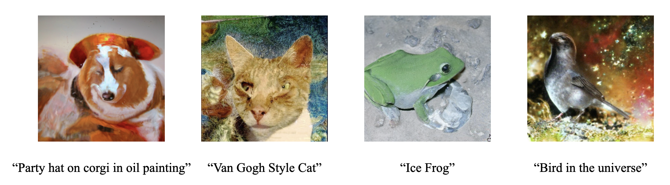
Figure 6: CLIP-guided demo figures

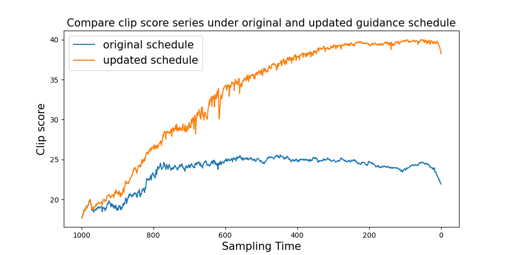
Figure 7: The comparison of CLIP scores series under linear guidance schedule and updated guidance schedule with sine factor during the sampling process.

6 Discussion

In this work, we elucidate the design space of off-the-shelf classifier guidance in diffusion generation. Using our training-free and accessible designs, off-the-shelf classifiers can effectively guide conditional diffusion, achieving state-of-the-art performance in ImageNet 128x128. Our approach is applicable to various diffusion models such as DDPM, EDM, and DiT, as well as text-to-image scenarios. We believe our work contributes significantly to the investigation of the ideal guidance method for diffusion models that may greatly benefit the booming AIGC industry.

There are multiple directions to extend this work. First, we primarily investigated classifier guidance in diffusion generation while there are more sophisticated discriminative models, e.g., detection models and visual Question Answering models, as well as other types of generative methods, e.g., masked image modeling (Chang et al., 2022, 2023) and autoregressive models (Esser et al., 2021; Yu et al., 2022, 2023). It would be interesting to explore other types of guided generation. Second, we only considered image generative models, and extending to language models would also be a promising direction. We believe that our proposed designs and calibration methodology hold potential for diverse modalities and we leave this for future work.

Appendix

Appendix A Classifier Design Space

A.1 Integral Calibration

To justify how the ECE calibration can help improve the guided sampling, we conduct a comparative analysis in different settings of classifiers in guided sampling in Table 2 based on Figure 1. In addition to the fine-tuned classifier and the off-the-shelf ResNet options, we introduce the ResNet&fine-tuned classifier combination. This combination utilizes ResNet guidance from 250 to 50 timesteps and fine-tuned classifier guidance from 50 to 0 timesteps, resulting in a lower ECE curve over time. The ResNet&fine-tuned combination demonstrates that lower ECE calibration error leads to improved guided sampling quality (lower FID(Heusel et al., 2017)). (Note: the ResNet&fine-tuned combination is used for demonstration purposes only, and we will solely employ the off-the-shelf ResNet in the subsequent analysis and guided sampling). We use the official ResNet checkpoints as the off-the-shelf classifier.

A.2 Ablation Study Details

In ablation study of Tables 1,3,4,5,6,A.1. The classifier is the official ResNet Pytorch checkpoint, the diffusion model is from Dhariwal and Nichol (2021) and the dataset is ImageNet 128x128. Generating 10000 samples with 250 DDPM steps for evaluation.

Table A.1: Comparative analysis of inputs in guided sampling with respect to $\text{ECE}_{t}$. The ResNet is the official Pytorch ResNet checkpoint; the diffusion model is from Dhariwal and Nichol (2021) and the dataset is ImageNet 128x128.

	$t=0$	$t=20$	$t=40$	$t=60$	$t=80$
$\text{ECE}_{t}$ $\widehat{x}_{t}$	0.25	0.41	0.46	0.39	0.31
$\text{ECE}_{t}$ $\widehat{x}_{0}(t)$	0.25	0.25	0.28	0.30	0.33

Appendix B Joint vs Conditional Probability

Figure B.1 presents the intermediate sampling images and the classifier gradient figures over 250 DDPM steps. Figure B.1 (a) represents the traditional conditional probability settings ($\tau_{1}=1,\tau_{2}=1$): the classifier gradient figure gradually fades from t=50 to 0, indicating a loss of object depiction guidance during the sampling. In contrast, Figure B.1 (b) showcases strengthened joint guidance ($\tau_{1}=1,\tau_{2}=0.5$): the classifier gradient figure increasingly highlights the object outline, providing consistent and accurate guidance direction throughout the entire sampling process.

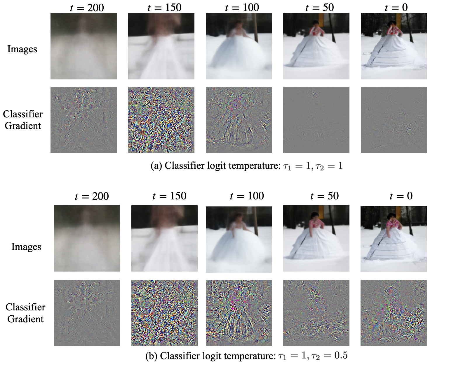
Figure B.1: The illustration of intermediate sampling images and classifier gradient figures under conditional probability guidance and joint guidance during the sampling process. The classifier is the official ResNet50 Pytorch checkpoint, the diffusion model is from Dhariwal and Nichol (2021) and the dataset is ImageNet 128x128. The seed is fixed for direct comparison.

Appendix C Experiment details

C.1 Experiment Details

The off-the-shelf classifiers are the official Pytorch checkpoints at: https://pytorch.org/vision/main/models/resnet.html.

Specifically, the ResNet50 checkpoint is at: https://download.pytorch.org/models/resnet50-11ad3fa6.pth; ResNet101 checkpoint is at: https://download.pytorch.org/models/resnet101-cd907fc2.pth.

To replicate the DDPM off-the-shelf classifier guided sampling in Table 7:

Softplus $\beta=3$, joint logit temperature $\tau_{1}=1.0$, marginal logit temperature $\tau_{2}=0.5$, classifier guidance schedule added Sine factor $\gamma_{t}=0.3$.

To replicate the EDM off-the-shelf classifier guided sampling in Table 8:

Softplus $\beta=5$, joint logit temperature $\tau_{1}=1.0$, marginal logit temperature $\tau_{2}=0.0$, classifier guidance schedule added sine factor $\gamma_{t}=0.3$. The guidance scale is 0.004 for 10 and 18 sampling steps, 0.0018 for 36 sampling steps, and 0.001 for 250 sampling steps.

To replicate the DiT off-the-shelf classifier guided sampling in Table 9:

classifier-free scale $s=1.5$, Softplus $\beta=6$, joint logit temperature $\tau_{1}=1.1$, marginal logit temperature $\tau_{2}=0.5$, classifier guidance schedule added sine factor $\gamma_{t}=0.2$,

C.2 More Experiments

The EDM off-the-shelf classifier guided sampling in 250 steps of SDE sampling on ImageNet 64x64 Kingma and Gao (2023) is presented in Table C.1 of Appendix C.2.

Table C.1: EDM baseline and the off-the-shelf ResNet guided EDM sampling. Sampled for 256 SDE steps. Generating 50000 ImageNet 64x64 samples for evaluation.

ImageNet 64x64	Classifier	FID
EDM baseline	-	1.41
EDM Res101 guided	Off-the-Shelf	1.33

Appendix D CLIP-guided Figures

The illustration of CLIP-guided diffusion sampling figures. The CLIP is the ViT-L(336px), and the diffusion model Dhariwal and Nichol (2021) is from 256x256 ImagNet.

$$\widehat{x}_{0}(t) =(\widehat{x}_{t}-(\sqrt{1-\alpha_{t}}\epsilon_{t}(\widehat{x}_{t})))/\sqrt{\alpha_{t}}$$ (D.1)

$$\mu_{t}(\text{guide}) =\mu_{t}(\widehat{x}_{t})+\gamma_{t}\nabla\text{CLIP}(\widehat{x}_{0}(t),prompt)$$

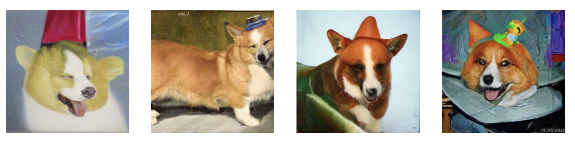
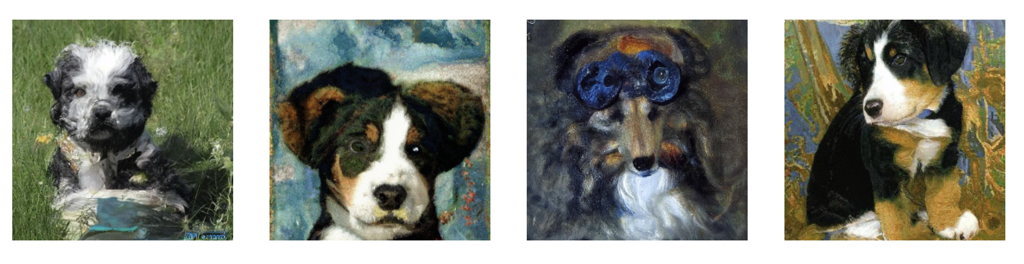
Figure D.1: "Party hat on corgi in oil painting"

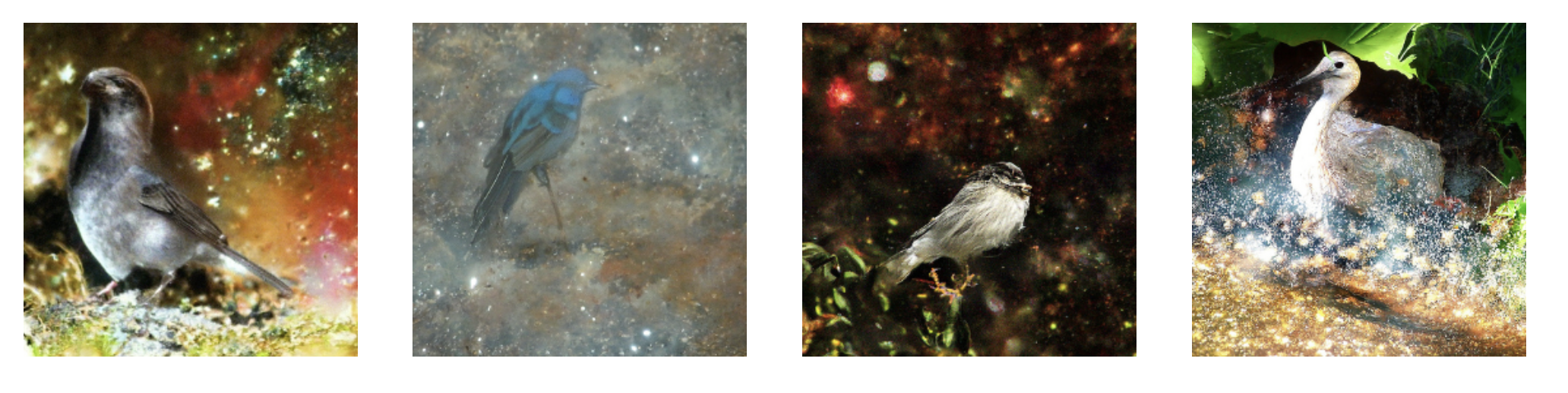
Figure D.2: "Van Gogh Style Dog"

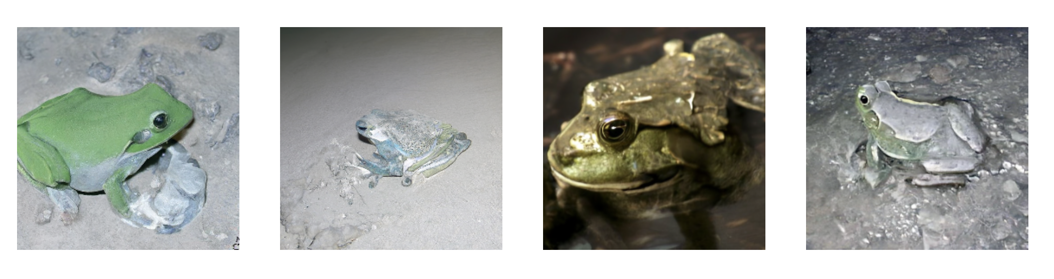
Figure D.3: "Bird in the universe"

Figure D.4: "Ice Frog"

Appendix E Proof of Proposition 4.1

This is a direct result of the interpolation inequality (Brezis and Mironescu, 2019). Specifically, the interpolation inequality implies that for any $f\in\mathcal{H}^{k}(\Omega)$, we have

$$\|\nabla f\|_{L_{2}(\Omega)}\leq C_{1}\|f\|_{\mathcal{H}^{k}(\Omega)}^{\frac{1}{k}}\|f\|_{L_{2}(\Omega)}^{1-\frac{1}{k}},$$

and

$$\|f\|_{L_{\infty}(\Omega)}\leq C_{2}\|f\|_{\mathcal{H}^{k}(\Omega)}^{\frac{d}{2k}}\|f\|_{L_{2}(\Omega)}^{1-\frac{d}{2k}},$$

where $C_{1},C_{2}$ are constants not depending on $f$, and $d$ is the dimension of the input $\bm{x}$. Let $\epsilon=p-p_{n}$, which satisfies

$$\|p-p_{n}\|_{L_{\infty}(\Omega)}\leq C_{2}C_{3}\|\epsilon\|_{\mathcal{H}^{k}(\Omega)}^{\frac{d}{2k}}\|\epsilon\|_{L_{2}(\Omega)}^{1-\frac{d}{2k}}=o_{\mathbb{P}}(1).$$ (E.1)

Also, we have

$$\|\nabla p-\nabla p_{n}\|_{L_{2}(\Omega)}\leq C_{1}\|\epsilon\|_{\mathcal{H}^{k}(\Omega)}^{\frac{1}{k}}\|\epsilon\|_{L_{2}(\Omega)}^{1-\frac{1}{k}}=o_{\mathbb{P}}(1).$$ (E.2)

Thus, it can be shown that

$$\|\nabla\log p-\nabla\log p_{n}\|_{L_{2}(\Omega)}= \left\|\frac{\nabla p}{p}-\frac{\nabla p_{n}}{p_{n}}\right\|_{L_{2}(\Omega)}$$

$$= \left\|\frac{p_{n}\nabla p-p\nabla p_{n}}{p(p-\epsilon)}\right\|_{L_{2}(\Omega)}$$

$$\leq \frac{\|p_{n}-p\|_{L_{2}(\Omega)}\|\nabla p\|_{L_{2}(\Omega)}+\|p\|_{L_{2}(\Omega)}\|\nabla p-\nabla p_{n}\|_{L_{2}(\Omega)}}{\|p\|_{L_{\infty}(\Omega)}(c_{1}-\|\epsilon\|_{L_{\infty}(\Omega)})}$$

$$= o_{\mathbb{P}}(1),$$

where the last equality is because the Sobolev embedding theorem implies $\|\nabla p\|_{L_{2}(\Omega)}\leq C_{4}\|p\|_{\mathcal{H}^{k}(\Omega)}$, and by Eq.E.1 and Eq.E.2. This finishes the proof.

Appendix F Proof of Proposition 4.2

For notational simplicity, let $h_{l}(\bm{x})=P(Z=l|X=\bm{x})$ and $g_{l}(\bm{x})=P(Z=l,X=\bm{x})$. Taking the gradient with respect to $\bm{x}$, it can be seen that

$$\nabla h_{l}(\bm{x})= \nabla\left(\frac{g_{l}(\bm{x})}{f(\bm{x})}\right)$$

$$\propto \frac{b_{l}f_{l}(\bm{x})\bm{\Sigma}_{l}^{-1}(\bm{\mu}_{l}-\bm{x})f(\bm{x})-b_{l}f_{l}(\bm{x})(\sum_{k=1}^{K}b_{k}e^{-\frac{1}{2}(\bm{x}-\mu_{k})^{\top}\bm{\Sigma}_{k}^{-1}(\bm{x}-\mu_{k})}\Sigma_{k}^{-1}(\bm{\mu}_{k}-\bm{x}))}{f(\bm{x})^{2}}$$

$$\propto \bm{\Sigma}_{l}^{-1}(\bm{x}-\bm{\mu}_{l})f(\bm{x})-\sum_{k=1}^{K}b_{k}e^{-\frac{1}{2}(\bm{x}-\mu_{k})^{\top}\bm{\Sigma}_{k}^{-1}(\bm{x}-\mu_{k})}\Sigma_{k}^{-1}(\bm{\mu}_{k}-\bm{x})$$

$$\propto \sum_{k=1}^{K}b_{k}e^{-\frac{1}{2}(\bm{x}-\bm{\mu}_{k})^{\top}\bm{\Sigma}_{k}^{-1}(\bm{x}-\bm{\mu}_{k})}(\bm{\Sigma}_{l}^{-1}(\bm{x}-\bm{\mu}_{l})-\bm{\Sigma}_{k}^{-1}(\bm{x}-\bm{\mu}_{k})).$$

Direct computation shows that

$$\nabla g_{l}(\bm{x})=b_{l}f_{l}(\bm{x})\bm{\Sigma}_{l}^{-1}(\bm{\mu}_{l}-\bm{x})\propto\bm{\Sigma}_{l}^{-1}(\bm{\mu}_{l}-\bm{x}).$$

References

- Bansal et al. (2023) Arpit Bansal, Hong-Min Chu, Avi Schwarzschild, Soumyadip Sengupta, Micah Goldblum, Jonas Geiping, and Tom Goldstein. Universal guidance for diffusion models. In Proceedings of the IEEE/CVF Conference on Computer Vision and Pattern Recognition, pages 843–852, 2023.
- Brezis and Mironescu (2019) Haïm Brezis and Petru Mironescu. Where Sobolev interacts with Gagliardo–Nirenberg. Journal of Functional Analysis, 277(8):2839–2864, 2019.
- Chang et al. (2022) Huiwen Chang, Han Zhang, Lu Jiang, Ce Liu, and William T Freeman. Maskgit: Masked generative image transformer. In Proceedings of the IEEE/CVF Conference on Computer Vision and Pattern Recognition, pages 11315–11325, 2022.
- Chang et al. (2023) Huiwen Chang, Han Zhang, Jarred Barber, AJ Maschinot, Jose Lezama, Lu Jiang, Ming-Hsuan Yang, Kevin Murphy, William T Freeman, Michael Rubinstein, et al. Muse: Text-to-image generation via masked generative transformers. arXiv preprint arXiv:2301.00704, 2023.
- Chen et al. (2022) Sitan Chen, Sinho Chewi, Jerry Li, Yuanzhi Li, Adil Salim, and Anru R Zhang. Sampling is as easy as learning the score: theory for diffusion models with minimal data assumptions. arXiv preprint arXiv:2209.11215, 2022.
- Chen et al. (2023) Yimeng Chen, Tianyang Hu, Fengwei Zhou, Zhenguo Li, and Zhi-Ming Ma. Explore and exploit the diverse knowledge in model zoo for domain generalization. In International Conference on Machine Learning, pages 4623–4640. PMLR, 2023.
- Dhariwal and Nichol (2021) Prafulla Dhariwal and Alexander Nichol. Diffusion models beat gans on image synthesis. Advances in Neural Information Processing Systems, 34:8780–8794, 2021.
- Dong et al. (2022) Qishi Dong, Awais Muhammad, Fengwei Zhou, Chuanlong Xie, Tianyang Hu, Yongxin Yang, Sung-Ho Bae, and Zhenguo Li. Zood: Exploiting model zoo for out-of-distribution generalization. Advances in Neural Information Processing Systems Volume 35, 2022.
- Epstein et al. (2023) Dave Epstein, Allan Jabri, Ben Poole, Alexei A Efros, and Aleksander Holynski. Diffusion self-guidance for controllable image generation. arXiv preprint arXiv:2306.00986, 2023.
- Esser et al. (2021) Patrick Esser, Robin Rombach, and Bjorn Ommer. Taming transformers for high-resolution image synthesis. In Proceedings of the IEEE/CVF conference on computer vision and pattern recognition, pages 12873–12883, 2021.
- Grathwohl et al. (2019) Will Grathwohl, Kuan-Chieh Wang, Jörn-Henrik Jacobsen, David Duvenaud, Mohammad Norouzi, and Kevin Swersky. Your classifier is secretly an energy based model and you should treat it like one. arXiv preprint arXiv:1912.03263, 2019.
- Heusel et al. (2017) Martin Heusel, Hubert Ramsauer, Thomas Unterthiner, Bernhard Nessler, and Sepp Hochreiter. Gans trained by a two time-scale update rule converge to a local nash equilibrium. Advances in neural information processing systems, 30, 2017.
- Ho and Salimans (2022) Jonathan Ho and Tim Salimans. Classifier-free diffusion guidance. arXiv preprint arXiv:2207.12598, 2022.
- Ho et al. (2020) Jonathan Ho, Ajay Jain, and Pieter Abbeel. Denoising diffusion probabilistic models. Advances in Neural Information Processing Systems, 33:6840–6851, 2020.
- Ho et al. (2022a) Jonathan Ho, William Chan, Chitwan Saharia, Jay Whang, Ruiqi Gao, Alexey Gritsenko, Diederik P Kingma, Ben Poole, Mohammad Norouzi, David J Fleet, et al. Imagen video: High definition video generation with diffusion models. arXiv preprint arXiv:2210.02303, 2022a.
- Ho et al. (2022b) Jonathan Ho, Tim Salimans, Alexey Gritsenko, William Chan, Mohammad Norouzi, and David J Fleet. Video diffusion models. arXiv preprint arXiv:2204.03458, 2022b.
- Hu et al. (2023) Tianyang Hu, Fei Chen, Haonan Wang, Jiawei Li, Wenjia Wang, Jiacheng Sun, and Zhenguo Li. Complexity matters: Rethinking the latent space for generative modeling. arXiv preprint arXiv:2307.08283, 2023.
- Karras et al. (2022) Tero Karras, Miika Aittala, Timo Aila, and Samuli Laine. Elucidating the design space of diffusion-based generative models. In Proc. NeurIPS, 2022.
- Kingma and Gao (2023) Diederik P. Kingma and Ruiqi Gao. Variational diffusion models 2.0: Understanding diffusion model objectives as the elbo with simple data augmentation, 2023.
- Kingma and Welling (2013) Diederik P Kingma and Max Welling. Auto-encoding variational bayes. arXiv preprint arXiv:1312.6114, 2013.
- Lin et al. (2023) Chen-Hsuan Lin, Jun Gao, Luming Tang, Towaki Takikawa, Xiaohui Zeng, Xun Huang, Karsten Kreis, Sanja Fidler, Ming-Yu Liu, and Tsung-Yi Lin. Magic3d: High-resolution text-to-3d content creation. In Proceedings of the IEEE/CVF Conference on Computer Vision and Pattern Recognition, pages 300–309, 2023.
- Luo et al. (2023) Weijian Luo, Tianyang Hu, Shifeng Zhang, Jiacheng Sun, Zhenguo Li, and Zhihua Zhang. Diff-instruct: A universal approach for transferring knowledge from pre-trained diffusion models. arXiv preprint arXiv:2305.18455, 2023.
- Molad et al. (2023) Eyal Molad, Eliahu Horwitz, Dani Valevski, Alex Rav Acha, Y. Matias, Yael Pritch, Yaniv Leviathan, and Yedid Hoshen. Dreamix: Video diffusion models are general video editors. ArXiv, abs/2302.01329, 2023.
- Naeini et al. (2015) Mahdi Pakdaman Naeini, Gregory Cooper, and Milos Hauskrecht. Obtaining well calibrated probabilities using bayesian binning. In Proceedings of the AAAI conference on artificial intelligence, volume 29, 2015.
- Nair and Hinton (2010) Vinod Nair and Geoffrey E Hinton. Rectified linear units improve restricted boltzmann machines. In Proceedings of the 27th international conference on machine learning (ICML-10), pages 807–814, 2010.
- Nichol and Dhariwal (2021) Alex Nichol and Prafulla Dhariwal. Improved denoising diffusion probabilistic models. arXiv preprint arXiv:2102.09672, 2021.
- Nichol et al. (2021) Alex Nichol, Prafulla Dhariwal, Aditya Ramesh, Pranav Shyam, Pamela Mishkin, Bob McGrew, Ilya Sutskever, and Mark Chen. Glide: Towards photorealistic image generation and editing with text-guided diffusion models. arXiv preprint arXiv:2112.10741, 2021.
- Peebles and Xie (2022) William Peebles and Saining Xie. Scalable diffusion models with transformers. arXiv preprint arXiv:2212.09748, 2022.
- Poole et al. (2022) Ben Poole, Ajay Jain, Jonathan T Barron, and Ben Mildenhall. Dreamfusion: Text-to-3d using 2d diffusion. arXiv preprint arXiv:2209.14988, 2022.
- Radford et al. (2021) Alec Radford, Jong Wook Kim, Chris Hallacy, Aditya Ramesh, Gabriel Goh, Sandhini Agarwal, Girish Sastry, Amanda Askell, Pamela Mishkin, Jack Clark, et al. Learning transferable visual models from natural language supervision. In International conference on machine learning, pages 8748–8763. PMLR, 2021.
- Ramesh et al. (2021) Aditya Ramesh, Mikhail Pavlov, Gabriel Goh, Scott Gray, Chelsea Voss, Alec Radford, Mark Chen, and Ilya Sutskever. Zero-shot text-to-image generation. In International Conference on Machine Learning, pages 8821–8831. PMLR, 2021.
- Ramesh et al. (2022) Aditya Ramesh, Prafulla Dhariwal, Alex Nichol, Casey Chu, and Mark Chen. Hierarchical text-conditional image generation with clip latents. arXiv preprint arXiv:2204.06125, 2022.
- Rombach et al. (2022) Robin Rombach, Andreas Blattmann, Dominik Lorenz, Patrick Esser, and Björn Ommer. High-resolution image synthesis with latent diffusion models. In Proceedings of the IEEE/CVF Conference on Computer Vision and Pattern Recognition, pages 10684–10695, 2022.
- Ronneberger et al. (2015) Olaf Ronneberger, Philipp Fischer, and Thomas Brox. U-net: Convolutional networks for biomedical image segmentation. In Medical Image Computing and Computer-Assisted Intervention–MICCAI 2015: 18th International Conference, Munich, Germany, October 5-9, 2015, Proceedings, Part III 18, pages 234–241. Springer, 2015.
- Saharia et al. (2022) Chitwan Saharia, William Chan, Saurabh Saxena, Lala Li, Jay Whang, Emily Denton, Seyed Kamyar Seyed Ghasemipour, Burcu Karagol Ayan, S Sara Mahdavi, Rapha Gontijo Lopes, et al. Photorealistic text-to-image diffusion models with deep language understanding. arXiv preprint arXiv:2205.11487, 2022.
- Shu et al. (2021) Yang Shu, Zhi Kou, Zhangjie Cao, Jianmin Wang, and Mingsheng Long. Zoo-tuning: Adaptive transfer from a zoo of models. In International Conference on Machine Learning, pages 9626–9637. PMLR, 2021.
- Singer et al. (2022) Uriel Singer, Adam Polyak, Thomas Hayes, Xi Yin, Jie An, Songyang Zhang, Qiyuan Hu, Harry Yang, Oron Ashual, Oran Gafni, et al. Make-a-video: Text-to-video generation without text-video data. arXiv preprint arXiv:2209.14792, 2022.
- Sohl-Dickstein et al. (2015) Jascha Sohl-Dickstein, Eric Weiss, Niru Maheswaranathan, and Surya Ganguli. Deep unsupervised learning using nonequilibrium thermodynamics. In International Conference on Machine Learning, pages 2256–2265. PMLR, 2015.
- Song et al. (2020a) Jiaming Song, Chenlin Meng, and Stefano Ermon. Denoising diffusion implicit models. arXiv preprint arXiv:2010.02502, 2020a.
- Song et al. (2020b) Yang Song, Jascha Sohl-Dickstein, Diederik P Kingma, Abhishek Kumar, Stefano Ermon, and Ben Poole. Score-based generative modeling through stochastic differential equations. In International Conference on Learning Representations, 2020b.
- Vahdat et al. (2021) Arash Vahdat, Karsten Kreis, and Jan Kautz. Score-based generative modeling in latent space. Advances in Neural Information Processing Systems, 34:11287–11302, 2021.
- Wallace et al. (2023) Bram Wallace, Akash Gokul, Stefano Ermon, and Nikhil Naik. End-to-end diffusion latent optimization improves classifier guidance. arXiv preprint arXiv:2303.13703, 2023.
- Wang et al. (2023) Zhengyi Wang, Cheng Lu, Yikai Wang, Fan Bao, Chongxuan Li, Hang Su, and Jun Zhu. Prolificdreamer: High-fidelity and diverse text-to-3d generation with variational score distillation. arXiv preprint arXiv:2305.16213, 2023.
- Yu et al. (2022) Jiahui Yu, Yuanzhong Xu, Jing Yu Koh, Thang Luong, Gunjan Baid, Zirui Wang, Vijay Vasudevan, Alexander Ku, Yinfei Yang, Burcu Karagol Ayan, et al. Scaling autoregressive models for content-rich text-to-image generation. arXiv preprint arXiv:2206.10789, 2(3):5, 2022.
- Yu et al. (2023) Lili Yu, Bowen Shi, Ramakanth Pasunuru, Benjamin Muller, Olga Golovneva, Tianlu Wang, Arun Babu, Binh Tang, Brian Karrer, Shelly Sheynin, et al. Scaling autoregressive multi-modal models: Pretraining and instruction tuning. arXiv preprint arXiv:2309.02591, 2023.
- Zhu et al. (2021) Yao Zhu, Jiacheng Sun, and Zhenguo Li. Rethinking adversarial transferability from a data distribution perspective. In International Conference on Learning Representations, 2021.