Diffractive single hadron production in a saturation framework at the NLO

Abstract

We calculate the cross-sections of diffractive single hadron photo- or electroproduction with large $p_{T}$, on a nucleon or a nucleus in the shockwave formalism. We use the hybrid formalism mixing collinear factorization with high energy small-$x$ factorization with the impact factors computed at next-to-leading order accuracy. We prove the cancellation of divergence and we determine the finite parts of the differential cross-sections. We work in general kinematics such that both photoproduction and leptoproduction are considered. The results can be used to detect saturation effects, at both the future EIC or already at LHC, using Ultra-Peripheral Collisions.

1 Introduction

Gluonic saturation effects in scattering on nucleons and nuclei at small-$x$ represent one of the most intriguing phenomena of strong interactions. In the small-$x$ kinematics, the BFKL dynamics Fadin:1975cb ; Kuraev:1976ge ; Kuraev:1977fs ; Balitsky:1978ic ; Fadin:1998py ; Ciafaloni:1998gs ; Fadin:2004zq ; Fadin:2005zj predicts a power-like increase of total cross sections at low values of the Bjorken variable $x=Q^{2}/s$, where $s$ is the center of mass and $Q^{2}$ an hard scale. This rise of cross-section is physically interpretable as a constant growth of the gluon density inside the proton. Although this growth has been experimentally observed, confirming the robustness of the BFKL approach, it is equally clear that it must necessarily be interpreted as a pre-asymptotic regime. In fact, at very low values of the $x$ variable, the parton density, per unit of transversal area, in the hadronic wave functions becomes very large leading to the so-called recombination effects (not included in the BFKL dynamics). When gluon recombination balances gluon splitting, the density of the latter reaches a saturation point, producing new and universal properties of hadronic matter. The state of gluonic matter that is formed is known as color-glass condensate McLerran:1993ni . The evolution of parton densities must then be described by nonlinear generalizations of the BFKL equation, i.e. the Balitsky — Jalilian Marian-Iancu-McLerran-Weigert-Leonidov-Kovner (B—JIMWLK) equations Balitsky:1995ub ; Balitsky:1998kc ; Balitsky:1998ya ; Balitsky:2001re ; JalilianMarian:1997jx ; JalilianMarian:1997gr ; JalilianMarian:1997dw ; JalilianMarian:1998cb ; Kovner:2000pt ; Weigert:2000gi ; Iancu:2000hn ; Iancu:2001ad ; Ferreiro:2001qy . In practice, we will rely on the Balitsky shockwave formulation.

In the present article, we extend a series of works by us devoted to a complete Next-to-Leading Order (NLO) description of the direct coupling of the Pomeron to several kinds of diffractive states, namely exclusive diffractive dijet production Boussarie:2014lxa ; Boussarie:2016ogo ; Boussarie:2019ero , exclusive $\rho$-meson production Boussarie:2016bkq , double hadron production at large $p_{T}$ Fucilla:2022wcg .

In the same spirit as in Ref. Fucilla:2022wcg , this study is motivated by present and future possibilities of accessing gluonic saturation through large-$p_{T}$ single hadron production. The novelty of the present study, as we will show in detail in this article, is that passing from dihadron to single hadron production, i.e. increasing the level of inclusivity, changes rather significantly the structure of the cancelation of IR divergencies. At the parton level, one indeed faces contributions with one (at LO and NLO) or two (at NLO) spectator partons, contrarily to the case of dihadron production.

Similarly to the case of dihadron production, this process could be studied both in photoproduction and leptoproduction. One should focus on the window which is both perturbative, the hard scale being provided either by the large virtuality $Q^{2}$ of the virtual photon (in the leptoproduction case) and/or the large $p_{T}$ of the produced hadron, and subject to saturation effects, characterized by the scale $Q_{s}^{2}\simeq(A/x)^{1/3}$ where $A$ is the mass number of the nucleus. This could thus be achieved at the LHC in $pA$ and $AA$ scattering, using Ultra-Peripheral Collisions (UPC), as well as at the EIC, where both photoproduction and leptoproduction could be considered.

2 Theoretical framework

2.1 Hybrid collinear/high-energy factorization

In the present paper, we focus on the computation at full NLO of the semi-inclusive diffractive hadron production in the high energy limit, namely

$$\gamma^{(*)}(p_{\gamma})+P(p_{0})\rightarrow h(p_{h})+X+P^{\prime}(p_{0^{\prime}})$$ (1)

where $P$ is a nucleon or a nucleus target, generically called proton in the following. The initial photon plays the role of a probe (also named projectile). Our computation applies both to the photoproduction case (including ultra-peripheral collisions) and to the electroproduction case (e.g. at EIC). A gap in rapidity is assumed between the outgoing nucleon/nucleus $(P^{\prime})$ and the diffractive system $(Xh)$. This is illustrated by Fig. 1.

Figure 1: Left: An example of amplitude of the process (1) at LO. Right: An example of amplitude contributing to the process (1) at NLO. The grey blob symbolizes the QCD shockwave. The double line symbolizes the target, which remains intact in the figure, but could just as well break. The quark and the antiquark fragment into the systems $(hX)$ (in the specific diagram $h$ is produced by the quark, but can be as well produced by the anti-quark). The tagged hadron $h$ is drawn in red.

We will be working in a combination of collinear factorization and small-$x$ factorization, more precisely in the shockwave formalism for the latter.

Kinematics

We introduce a light-cone basis composed of $n_{1}$ and $n_{2}$, with $n_{1}\cdot n_{2}=1$ defining the $+/-$ direction. We write the Sudakov decomposition for any vector as

$$p^{\mu}=p^{+}n_{1}^{\mu}+p^{-}n_{2}^{\mu}+p_{\perp}^{\mu}$$ (2)

and the scalar product of two vectors as

$$p\cdot q =p^{+}q^{-}+p^{-}q^{+}+p_{\perp}\cdot q_{\perp}$$ (3)

$$=p^{+}q^{-}+p^{-}q^{+}-\vec{p}\cdot\vec{q}\,.$$

We work in a reference frame, called probe frame such that the target moves ultra-relativistically and such that $s=(p_{\gamma}+p_{0})^{2}\sim 2p_{\gamma}^{+}p_{0}^{-}\gg\Lambda_{\text{QCD}}^{2}$, $s$ also being larger than any other scale and $p_{\gamma}^{+}\sim p_{0}^{-}\sim\sqrt{s}$. Particles on the projectile side are moving in the $n_{1}$ (i.e. $+$) direction while particles on the target side have a large component along $n_{2}$ (i.e. $-$ direction).

We will use kinematics such that the photon with virtuality $Q$ is forward, and thus it does not carry any transverse momentum:

$$\vec{p}_{\gamma}=0,\quad p_{\gamma}^{\mu}=p_{\gamma}^{+}n_{1}^{\mu}+\frac{p_{\gamma}^{2}}{2p_{\gamma}^{+}}n_{2}^{\mu},\quad-p_{\gamma}^{2}\equiv Q^{2}\geq 0.$$ (4)

We will denote its transverse polarization $\varepsilon_{T}$. Its longitudinal polarization vector reads

$$\varepsilon_{L}^{\alpha}=\frac{1}{\sqrt{-p_{\gamma}^{2}}}\left(p_{\gamma}^{+}n_{1}^{\alpha}-\frac{p_{\gamma}^{2}}{2p_{\gamma}^{+}}n_{2}^{\alpha}\right),\quad\varepsilon_{L}^{+}=\frac{p_{\gamma}^{+}}{Q},\quad\varepsilon_{L}^{-}=\frac{Q}{2p_{\gamma}^{+}}.$$ (5)

We write the momentum of the produced hadron as

$$p^{\mu}_{h}=p^{+}_{h}n_{1}^{\mu}+\frac{m_{h}^{2}+\vec{p}_{h}^{\,2}}{2p^{+}_{h}}n_{2}^{\mu}+p^{\mu}_{h\perp}\,.$$ (6)

The momenta of the fragmenting quark of virtuality $p_{q}^{2}$ reads

$$p^{\mu}_{q}=p^{+}_{q}n_{1}^{\mu}+\frac{p_{q}^{2}+\vec{p}_{q}^{\,2}}{2p^{+}_{q}}n_{2}^{\mu}+p^{\mu}_{q\perp}\,,$$ (7)

similarly for an antiquark of virtuality $p_{\bar{q}}^{2}$ we have

$$p^{\mu}_{\bar{q}}=p^{+}_{\bar{q}}n_{1}^{\mu}+\frac{p^{2}_{\bar{q}}+\vec{p}_{\bar{q}}^{\,2}}{2p^{+}_{\bar{q}}}n_{2}^{\mu}+p^{\mu}_{\bar{q}\perp}\,,$$ (8)

and, finally, for a gluon appearing at NLO level, we can write

$$p^{\mu}_{g}=p^{+}_{g}n_{1}^{\mu}+\frac{p^{2}_{g}+\vec{p}_{g}^{\,2}}{2p^{+}_{g}}n_{2}^{\mu}+p^{\mu}_{g\perp}\,.$$ (9)

From now, we will use the notation $p_{ij}=p_{i}-p_{j}$ and $z_{ij}=z_{i}-z_{j}$.

Collinear factorization

We consider the kinematical region in which $\vec{p}_{h}^{\,2}\gg\Lambda_{\text{QCD}}^{2}$. This transverse hadron momentum provides the hard scale, justifying the use of perturbative QCD and collinear factorization. In the hard part, after collinear factorization, the quark and antiquark can be treated as on-shell particles. We later on use the longitudinal momentum fraction $x_{q}$ and $x_{\bar{q}}$, defined as

$$p_{q}^{+}=x_{q}p^{+}_{\gamma}\quad\hbox{ and }\quad p_{\bar{q}}^{+}=x_{\bar{q}}p^{+}_{\gamma}\,.$$ (10)

We also denote

$$p_{h}^{+}=x_{h}p^{+}_{\gamma}\,.$$ (11)

Shockwave approach

We now shortly present the shockwave formalism, an effective approach to deal with gluonic saturation.

In this effective field theory, the gluonic field $A$ is separated into external background fields $b$ (resp. internal fields $\mathcal{A}$) depending on whether their $+$-momentum is below (resp. above) the arbitrary rapidity cut-off $e^{\eta}p_{\gamma}^{+}$, with $\eta<0$. This effective field theory dramatically simplifies when using the light-cone gauge $n_{2}\cdot A=0$. The external fields, after being highly boosted from the target rest frame to the probe frame, take the form

$$b^{\mu}(x)=b^{-}(x_{\perp})\delta(x^{+})n_{2}^{\mu}\,.$$ (12)

The resummation of all order interactions with those fields leads to a high-energy Wilson line, that represents the shockwave and is located exactly at $x^{+}=0$:

$$U_{\vec{z}}=\mathcal{P}\exp\left(ig\int dz^{+}b^{-}(z)\right)\,,$$ (13)

where $\mathcal{P}$ is the usual path ordering operator for the $+$ direction.

Relying on the small-$x$ factorization, the scattering amplitude can be written as the convolution of the projectile impact factor with the non-perturbative matrix element of operators from the Wilson line operators on the target states.

For the present process, we will deal with two kinds of operators. The first one is the dipole operator, which in the fundamental representation of $SU(N_{c})$ takes the form:

$$\left[\operatorname{Tr}\left(U_{1}U_{2}^{\dagger}\right)-N_{c}\right]\left(\vec{p_{1}},\vec{p}_{2}\right)=\int d^{d}\vec{z}_{1}d^{d}\vec{z}_{2\perp}e^{-i\vec{p}_{1}\cdot\vec{z}_{1}}e^{-i\vec{p}_{2}\cdot\vec{z}_{2}}\left[\operatorname{Tr}\left(U_{\vec{z}_{1}}U_{\vec{z}_{2}}^{\dagger}\right)-N_{c}\right]\,,$$ (14)

where $\vec{z}_{1,2}$ are the transverse positions of the $q,\bar{q}$ coming from the photon and $\vec{p}_{1,2}$ their respective transverse momentums kicks from the shockwave.

The proton matrix element can be parameterized through a generic function $F$, following the definition of Ref. Boussarie:2016ogo

$$\left\langle P^{\prime}\left(p_{0^{\prime}}\right)\left|T\left(\operatorname{Tr}\left(U_{\frac{z_{\perp}}{2}}U_{-\frac{z_{\perp}}{2}}^{\dagger}\right)-N_{c}\right)\right|P\left(p_{0}\right)\right\rangle \equiv 2\pi\delta\left(p_{00^{\prime}}^{-}\right)F_{p_{0\perp}p_{0^{\prime}\perp}}\left(z_{\perp}\right)$$ (15)

$$\equiv 2\pi\delta\left(p_{00^{\prime}}^{-}\right)F\left(z_{\perp}\right)$$

and its Fourier Transform (FT) is

$$\int d^{d}z_{\perp}e^{i\left(z_{\perp}\cdot p_{\perp}\right)}F\left(z_{\perp}\right)\equiv\mathbf{F}\left(p_{\perp}\right).$$ (16)

The second operator we will deal with is the double dipole operator. Its action on proton states, as can be seen with eqs. (5.3) and (5.6) in Boussarie:2016ogo , can be written as

$$\left\langle P^{\prime}\left(p_{0^{\prime}}\right)\left|\left(\operatorname{Tr}\left(U_{\frac{z_{\perp}}{2}}U_{x_{\perp}}^{\dagger}\right)\operatorname{Tr}\left(U_{x_{\perp}}U_{-\frac{z_{\perp}}{2}}^{\dagger}\right)-N_{c}\operatorname{Tr}\left(U_{\frac{z_{\perp}}{2}}U_{-\frac{z_{\perp}}{2}}^{\dagger}\right)\right)\right|P\left(p_{0}\right)\right\rangle$$

$$\equiv 2\pi\delta\left(p_{00^{\prime}}^{-}\right)\tilde{F}_{p_{0\perp}p_{0^{\prime}\perp}}\left(z_{\perp},x_{\perp}\right)\equiv 2\pi\delta\left(p_{00^{\prime}}^{-}\right)\tilde{F}\left(z_{\perp},x_{\perp}\right)$$ (17)

and its FT is

$$\int d^{d}z_{\perp}d^{d}x_{\perp}e^{i\left(p_{\perp}\cdot x_{\perp}\right)+i\left(z_{\perp}\cdot q_{\perp}\right)}\tilde{F}\left(z_{\perp},x_{\perp}\right)\equiv\tilde{\mathbf{F}}\left(q_{\perp},p_{\perp}\right).$$ (18)

In this paper, dimensional regularization will be used with $D=2+d$, where $d=2+2\epsilon$ is the transverse dimension.

2.2 LO computation

Figure 2: Graphical convention for the fragmentation function of a parton (here a quark for illustration) to a hadron $h$ plus spectators. In the rest of this article, we will use the left-hand side of this drawing.

We start from the usual collinear factorization of the hadronic cross section for the production of a single hadron which, at LO and leading twist, reads Altarelli:1979kv

$$\frac{d\sigma_{0JI}^{q\rightarrow h}}{dx_{h}}=\sum_{q}\int_{x_{h}}^{1}\frac{dx_{q}}{x_{q}}D_{q}^{h}\left(\frac{x_{h_{1}}}{x_{q}},\mu_{F}\right)\frac{d\hat{\sigma}_{0JI}}{dx_{q}}\;,$$ (19)

where $q$ specifies the quark or anti-quark flavor types ($q=u,\bar{u},d,\bar{d},s,\bar{s},c,\bar{c},b,\bar{b}$), and $J,I=L,T$ specify the photon polarization since we deal here with a modulus square amplitude ($J$ labels the photon polarization in the complex conjugated amplitude and $I$ in the amplitude). Here $\mu_{F}$ is the factorization scale, $D_{q}^{h}$ denotes the quark (or antiquark) Fragmentation Function (FF) and $d\hat{\sigma}$ is the cross-section for the production of partons, i.e. the cross-section for the subprocess

$$\gamma^{(*)}(p_{\gamma})+P(p_{0})\rightarrow q(p_{q})+\bar{q}(p_{\bar{q}})+P^{\prime}(p_{0^{\prime}})\,.$$ (20)

Following the convention of our previous work Fucilla:2022wcg we denote the fragmentation process by a small rectangle as in Fig. 2.

For illustrative purposes, and simplicity of notation, let us consider the case in which the hadron fragments starting from a quark. The case of anti-quark is completely identical. Collinear factorization means that the produced hadron should fly collinearly to the fragmenting parton, we then have the following constraints

$$p^{+}_{q} = \frac{x_{q}}{x_{h}}p^{+}_{h},\quad\vec{p}_{q}=\frac{x_{q}}{x_{h}}\vec{p}_{h}\,.$$ (21)

To keep things quite general with regard to photon polarization, and therefore to be able to describe photo- and electroproduction, we build the polarization matrix

$$d\sigma_{JI}=\begin{pmatrix}d\sigma_{LL}&d\sigma_{LT}\\ d\sigma_{TL}&d\sigma_{TT}\end{pmatrix},\qquad d\sigma_{TL}=d\sigma_{LT}^{\ast}\,.$$ (22)

Each element of this matrix has a LO contribution $d\sigma_{0JI}$. This Born order result, see Eq. (5.14) of Ref. Boussarie:2016ogo , has the following structure:

$$d\hat{\sigma}_{0JI} =\frac{\alpha_{\mathrm{em}}Q_{q}^{2}}{2\left(2\pi\right)^{4d}N_{c}}\frac{\left(p_{0}^{-}\right)^{2}}{2x_{q}x_{\bar{q}}s^{2}}dx_{q}dx_{\bar{q}}d^{d}p_{q\perp}d^{d}p_{\bar{q}\perp}\delta\left(1-x_{q}-x_{\bar{q}}\right)\left(\varepsilon_{I\beta}\varepsilon_{J\gamma}^{\ast}\right)$$

$$\quad\times\int d^{d}p_{1\perp}d^{d}p_{2\perp}d^{d}p_{1^{\prime}\perp}d^{d}p_{2^{\prime}\perp}\delta\left(p_{q1\perp}+p_{\bar{q}2\perp}\right)\delta\left(p_{11^{\prime}\perp}+p_{22^{\prime}\perp}\right)$$

$$\quad\times\sum_{\lambda_{q},\lambda_{\bar{q}}}\Phi_{0}^{\beta}\left(p_{1\perp},\,p_{2\perp}\right)\Phi_{0}^{\gamma*}\left(p_{1^{\prime}\perp},\,p_{2^{\prime}\perp}\right)\mathbf{F}\left(\frac{p_{12\perp}}{2}\right)\mathbf{F^{*}}\left(\frac{p_{1^{\prime}2^{\prime}\perp}}{2}\right).$$ (23)

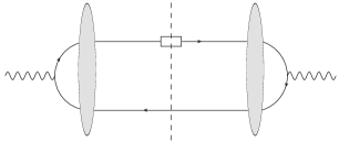
Figure 3: Diagram of the LO process at cross-section level. The blob is the shockwave (we do not draw the coupling with the target for clarity) and the square the FF, see Fig. 2. The dashed line represents the integration over phase space.

It is important to note that the formula (23) is divided by a factor of $1/(2(2\pi)^{4})$ with respect to Eq. (5.14) of Ref. Boussarie:2016ogo . This is necessary to get proper normalization which is missing in Ref. Boussarie:2016ogo due to a misprint. This same division must be applied to the cross section expressions in Ref. Fucilla:2022wcg , where this misprint propagated. Using the explicit expressions of the product $\Phi_{0}^{\beta}\Phi_{0}^{\gamma*}$, see Eqs. (115, 116, 117) in Appendix A, the LO cross-sections are obtained and read

$$\frac{d\sigma_{0JI}^{q\rightarrow h}}{dx_{h}d^{d}p_{h\perp}}=\frac{2\alpha_{\mathrm{em}}Q^{2}}{(2\pi)^{4d}N_{c}\;x_{h}^{d}}\sum_{q}Q_{q}^{2}\int_{x_{h}}^{1}dx_{q}\;x_{q}^{1+d}(1-x_{q})^{2}D_{q}^{h}\left(\frac{x_{h}}{x_{q}}\right)f_{JI}\,,$$ (24)

where

$$f_{LL}=\int d^{d}p_{\bar{q}\perp}\int d^{d}p_{2\perp}\frac{\mathbf{F}\left(\frac{x_{q}}{2x_{h}}p_{h\perp}+\frac{1}{2}p_{\bar{q}\perp}-p_{2\perp}\right)}{\vec{p}_{\bar{q}2}^{\;2}+x_{q}(1-x_{q})Q^{2}}\int d^{d}p_{2^{\prime}\perp}\frac{\mathbf{F}^{*}\left(\frac{x_{q}}{2x_{h}}p_{h\perp}+\frac{1}{2}p_{\bar{q}\perp}-p_{2^{\prime}\perp}\right)}{\vec{p}_{\bar{q}2^{\prime}}^{\;2}+x_{q}(1-x_{q})Q^{2}}\,,$$ (25)

$$f_{TL} =\int d^{d}p_{\bar{q}\perp}\int d^{d}p_{2\perp}\frac{\mathbf{F}\left(\frac{x_{q}}{2x_{h}}p_{h\perp}+\frac{1}{2}p_{\bar{q}\perp}-p_{2\perp}\right)}{\vec{p}_{\bar{q}2}^{\;2}+x_{q}(1-x_{q})Q^{2}}\int d^{d}p_{2^{\prime}\perp}\frac{\mathbf{F}^{*}\left(\frac{x_{q}}{2x_{h}}p_{h\perp}+\frac{1}{2}p_{\bar{q}\perp}-p_{2^{\prime}\perp}\right)}{\vec{p}_{\bar{q}2^{\prime}}^{\;2}+x_{q}(1-x_{q})Q^{2}}$$

$$\times\frac{(1-2x_{q})}{2x_{q}(1-x_{q})Q}\left(\vec{p}_{\bar{q}2^{\prime}}\cdot\vec{\varepsilon}_{T}\right)^{*}\;,$$ (26)

$$f_{TT} =\int d^{d}p_{\bar{q}\perp}\int d^{d}p_{2\perp}\frac{\mathbf{F}\left(\frac{x_{q}}{2x_{h}}p_{h\perp}+\frac{1}{2}p_{\bar{q}\perp}-p_{2\perp}\right)}{\vec{p}_{\bar{q}2}^{\;2}+x_{q}(1-x_{q})Q^{2}}\int d^{d}p_{2^{\prime}\perp}\frac{\mathbf{F}^{*}\left(\frac{x_{q}}{2x_{h}}p_{h\perp}+\frac{1}{2}p_{\bar{q}\perp}-p_{2^{\prime}\perp}\right)}{\vec{p}_{\bar{q}2^{\prime}}^{\;2}+x_{q}(1-x_{q})Q^{2}}$$

$$\times\left[(1-2x_{q})^{2}g_{\perp}^{ri}g_{\perp}^{lk}-g_{\perp}^{rk}g_{\perp}^{li}+g_{\perp}^{rl}g_{\perp}^{ik}\right]\frac{\varepsilon_{Ti}\;p_{\bar{q}2\perp r}\left(\varepsilon_{Tk}\;p_{\bar{q}2^{\prime}\perp l}\right)^{*}}{4x_{q}^{2}(1-x_{q})^{2}Q^{2}}\;,$$ (27)

are the three different functions for the $LL$, $TL$ and $TT$ cross-sections, respectively and the sum over $q$ is extended to the five quark flavor species ($q=u,d,s,c,b$). For compactness, we use the short notation

$$f_{JI}(x_{q},x_{h},\vec{p}_{h},Q^{2})\equiv f_{JI}\;.$$ (28)

The correct cross section, in the case of anti-quark fragmentation, is obtained by including a minus sign in the argument of the function F, extending the sum over $q$ to the five anti-quark flavor species ($q=\bar{u},\bar{d},\bar{s},\bar{c},\bar{b}$) and performing the relabelling $(x_{q},\vec{p}_{q},p_{2},p_{2^{\prime}})\leftrightarrow(x_{\bar{q}},\vec{p}_{\bar{q}},p_{1},p_{1^{\prime}})$. We will call this last operation $(q\leftrightarrow\bar{q})$ relabelling.

2.3 NLO computations in a nutshell

2.3.1 Different mechanisms of fragmentation

At the next-to-leading order there are six kinds of contributions to the cross-section

• $\gamma^{*}+P\rightarrow h+\bar{q}+X+P$ cross-section at one-loop (i.e. virtual contribution and fragmentation from a quark) ,

• $\gamma^{*}+P\rightarrow h+q+X+P$ cross-section at one-loop (i.e. virtual contribution and fragmentation from an anti-quark) ,

• $\gamma^{*}+P\rightarrow h+\bar{q}+g+X+P$ cross-section at Born level (i.e. real contribution and fragmentation from a quark) ,

• $\gamma^{*}+P\rightarrow h+q+g+X+P$ cross-section at Born level (i.e. real contribution and fragmentation from an anti-quark) ,

• $\gamma^{*}+P\rightarrow h+q+\bar{q}+X+P$ cross-section at Born level (i.e. real contribution and fragmentation from a gluon) ,

• FFs counterterms .

2.3.2 Hard cross section

At NLO, since we rely on the shockwave approach, it is convenient to separate the various contributions from the dipole point of view, as illustrated in Fig. 4. In this figure, we exhibit a few examples of diagrams, either virtual or real, as a representative of each 5 classes of diagrams. There are indeed 5 classes of contributions from the dipole point of view, namely $d\sigma_{iJI}\,(i=1,\cdots 5)$, so that the NLO polarization matrix can be written as

$$d\sigma_{JI}=d\sigma_{0JI}+d\sigma_{1JI}+d\sigma_{2JI}+d\sigma_{3JI}+d\sigma_{4JI}+d\sigma_{5JI}.$$ (29)

Now, we will shortly discuss each of these 5 NLO corrections.

For the virtual diagrams, there are two classes of diagrams: the diagrams in which the virtual gluon does not cross the shockwave, thus contributing to $d\sigma_{1IJ}$, purely made of dipole $\times$ dipole terms; the diagrams in which the virtual gluon does cross the shockwave, contributing both to $d\sigma_{1IJ}$, made of dipole $\times$ dipole terms as well as to $d\sigma_{2IJ}$, made of double dipole $\times$ dipole (and dipole $\times$ double dipole) terms.

For the real diagrams, there are three classes of diagrams: the diagrams in which the real gluon does not cross the shockwave, thus contributing to $d\sigma_{3IJ}$, purely made of dipole $\times$ dipole terms; the diagrams in which the real gluon crosses exactly once the shockwave, contributing both to $d\sigma_{3IJ}$, made of dipole $\times$ dipole terms as well as to $d\sigma_{4IJ}$, made of double dipole $\times$ dipole (and dipole $\times$ double dipole) terms; the diagrams in which the real gluon crosses exactly twice the shockwave, contributing to $d\sigma_{3IJ}$, made of dipole $\times$ dipole terms, to $d\sigma_{4IJ}$, made of double dipole $\times$ dipole (and dipole $\times$ double dipole) terms, and to $d\sigma_{5IJ}$, made of double dipole $\times$ double dipole terms.

We stress that in Fig. 4 we show the hard cross-section. In order to construct the quark (anti-quark) part of the physical cross-section, the five contributions must be convoluted with the quark (anti-quark) $\rightarrow$ hadron FF. To include the gluon contribution to the physical cross-section, only the three kinds of real corrections must be convoluted with the gluon $\rightarrow$ hadron FF.

Figure 4: Illustration of the 5 kinds of contributions to the NLO hard cross-section from the dipole point of view. Arrows show to which combination of dipole structures each type of diagrams contributes.

2.3.3 Rapidity divergences and UV-sector

The dipole $\times$ double dipole part of the virtual amplitude contains a rapidity divergences of the form $\ln\alpha$. The presence of the divergence in rapidity is a natural consequence of the separation between the impact factor and the target. Intuitively, a gluon crossing the shockwave cannot have arbitrarily small fraction of longitudinal momentum (and hence arbitrary small rapidity), because only gluon with positive $+$-momentum above the cut-off $\alpha p_{\gamma}^{+}$ can contribute to the quantum corrections to the impact factor. The rapidity divergent-terms have to be absorbed into the renormalized Wilson operators with the help of the B-JIMWLK equation. We thus have to use the B-JIMWLK evolution for these operators from the cutoff $\alpha$ to the rapidity divide $e^{\eta}$, by writing

$$\widetilde{\mathcal{U}}_{12}^{\alpha}=\widetilde{\mathcal{U}}_{12}^{e^{\eta}}-\int_{\alpha}^{e^{\eta}}d\rho\frac{\partial\widetilde{\mathcal{U}}_{12}}{\partial\rho}\;.$$ (30)

This operation, applied to the leading term, produces an additional next-to-leading contribution which cancels the rapidity divergences. In next-to-leading term, the effect is simply to replace the scale $\alpha$ with the scale $e^{\eta}$.

In principle, we should deal with ultraviolet renormalization, which is very challenging in non-covariant gauges, however, in the shockwave approach, the only UV-divergences at NLO are associated with the dressing of external states (e.g. quark self-energy). Since we treat both the ultraviolet (UV) and the infrared (IR) divergences using dimensional regularization, these singularities are of the type

$$\frac{1}{\epsilon_{UV}}-\frac{1}{\epsilon_{IR}}$$ (31)

and can be set to zero by choosing $\epsilon_{UV}=\epsilon_{IR}$. Then, in practice, some UV divergences will cancel out some infrared divergences in the calculation.

2.3.4 Treatment of the IR-sector

When generically decomposing any on-shell parton momentum in the Sudakov basis as

$$p^{\mu}=zp^{+}n_{1}^{\mu}+\frac{\vec{p}^{\,2}}{2zp^{+}}n_{2}^{\mu}+p_{\perp}^{\mu}\,,$$ (32)

in the IR sector, we face three kinds of divergences:

• Rapidity: $z$ goes to 0 and $p_{\perp}$ arbitrary.

• Soft: any component of the gluon momentum goes linearly to 0 (obtained with both $z$ and $p_{\perp}=z\tilde{p}_{\perp}\sim z$ going to 0).

• Collinear: parton’s $p_{\perp}$ goes to zero, $z$ being arbitrary.

Technically, as the integration over $z$ is regulated through a lower cut-off ($\alpha$), care must be taken that the appearance of $\ln\alpha$ can arise from both rapidity and soft divergences.

The calculation is organized as follows. First, the rapidity divergences, which appear only in the virtual corrections in the present computation, are regularized at the amplitude level by absorbing them in the shockwave through one step of B-JIMWLK evolution. Part of terms with $\ln\alpha$, the one related to pure rapidity divergences, are then removed. Soft divergences must cancel in the combination between real and virtual contributions as guaranteed by the Kinoshita-Lee-Naurenberg theorem. To observe easily the cancellation we separate the real cross-section into soft-divergent and soft-free part. Then, when the cancellation takes place, any dependence on $\alpha$ disappears. Finally, the remaining type of divergences, which are of purely collinear nature, will be cancelled performing the renormalization of FFs Gribov:1972ri ; Lipatov:1974qm ; Altarelli:1977zs ; Dokshitzer:1977sg .

Before calculating all contributions, we explicitly show how the final cross section is organized. We strongly rely on the separation of the hard cross-section in Eq. (29).

Quark fragmentation

Figure 5: Real diagrams with the gluon emitted after the shockwave, in the quark fragmentation case.

The virtual part of the cross-section, in the quark fragmentation case, can be split as

$$\frac{d\sigma_{JI}^{q\rightarrow h}}{dx_{h}d^{d}p_{h\perp}}\bigg{|}_{\text{virt., NLO}}=\frac{d\sigma_{JI}^{q\rightarrow h}}{dx_{h}d^{d}p_{h\perp}}\bigg{|}_{S_{V}}+\frac{d\sigma_{JI}^{q\rightarrow h}}{dx_{h}d^{d}p_{h\perp}}\bigg{|}_{\text{virt., dip. $\times$ dip.}}+\frac{d\sigma_{JI}^{q\rightarrow h}}{dx_{h}d^{d}p_{h\perp}}\bigg{|}_{\text{virt., dip. $\times$ d. dip.}},$$ (33)

where the first term contains the singular virtual dipole $\times$ dipole contribution, the second one contains the finite virtual dipole $\times$ dipole contribution and, finally, the last term contains the finite dipole $\times$ double dipole contribution (see the two top diagrams in Fig. 4). We observe that the latter contribution becomes completely finite once the rapidity divergences have been removed.

The real part of the cross-section in the quark fragmentation case can be split as

$$\frac{d\sigma_{JI}^{q\rightarrow h}}{dx_{h}d^{d}p_{h\perp}}\bigg{|}_{\text{real, NLO}}=\frac{d\sigma_{JI}^{q\rightarrow h}}{dx_{h}d^{d}p_{h\perp}}\bigg{|}_{\text{real, dip. $\times$ dip.}}$$

$$+\frac{d\sigma_{JI}^{q\rightarrow h}}{dx_{h}d^{d}p_{h\perp}}\bigg{|}_{\text{real, dip. $\times$ d. dip.}}+\frac{d\sigma_{JI}^{q\rightarrow h}}{dx_{h}d^{d}p_{h\perp}}\bigg{|}_{\begin{subarray}{c}\text{real,}\\ \text{d. dip. $\times$ d. dip.}\end{subarray}}\;,$$ (34)

where the splitting follows the separation illustrated in the bottom diagrams in Fig. 4. The last two contributions are finite, while the first one can be further divided into a singular and finite contribution,

$$\frac{d\sigma_{JI}^{q\rightarrow h}}{dx_{h}d^{d}p_{h\perp}}\bigg{|}_{\text{real, dip. $\times$ dip.}}=\frac{d\sigma_{JI}^{q\rightarrow h}}{dx_{h}d^{d}p_{h\perp}}\bigg{|}_{\begin{subarray}{c}\text{real, singular}\\ \text{dip. $\times$ dip.}\end{subarray}}+\frac{d\sigma_{JI}^{q\rightarrow h}}{dx_{h}d^{d}p_{h\perp}}\bigg{|}_{\begin{subarray}{c}\text{real, finite}\\ \text{dip. $\times$ dip.}\end{subarray}}\;.$$ (35)

The singular contribution is generated by the diagrams shown in Fig. 5. This contribution contains both soft and collinear singularity that can be promptly separated by casting the contribution into the following form (the labels $(i)$ refer to Fig. 5)

$$\frac{d\sigma_{JI}^{q\rightarrow h}}{dx_{h}d^{d}p_{h\perp}}\bigg{|}_{\begin{subarray}{c}\text{real, singular}\\ \text{dip. $\times$ dip.}\end{subarray}}=\frac{d\sigma_{JI}^{q\rightarrow h}}{dx_{h}d^{d}p_{h\perp}}\bigg{|}_{(1)}+\frac{d\sigma_{JI}^{q\rightarrow h}}{dx_{h}d^{d}p_{h\perp}}\bigg{|}_{(2)}+\frac{d\sigma_{JI}^{q\rightarrow h}}{dx_{h}d^{d}p_{h\perp}}\bigg{|}_{(3)}+\frac{d\sigma_{JI}^{q\rightarrow h}}{dx_{h}d^{d}p_{h\perp}}\bigg{|}_{(4)}$$ (36)

$$=\frac{d\sigma_{JI}^{q\rightarrow h}}{dx_{h}d^{d}p_{h\perp}}\bigg{|}_{\text{Soft}}+\frac{d\sigma_{JI}^{q\rightarrow h}}{dx_{h}d^{d}p_{h\perp}}\bigg{|}_{\text{coll}(qg)}+\frac{d\sigma_{JI}^{q\rightarrow h}}{dx_{h}d^{d}p_{h\perp}}\bigg{|}_{\text{coll}(\bar{q}g)}+\frac{d\sigma_{JI}^{q\rightarrow h}}{dx_{h}d^{d}p_{h\perp}}\bigg{|}_{\text{real, fin. sub.}}\,.$$ (37)

The first contribution contains the sum of the four diagrams in the soft limit, i.e.

$$\frac{d\sigma_{JI}^{q\rightarrow h}}{dx_{h}d^{d}p_{h\perp}}\bigg{|}_{\text{Soft}}\equiv\frac{d\sigma_{JI}^{q\rightarrow h}}{dx_{h}d^{d}p_{h\perp}}\bigg{|}_{(1),\text{Soft}}+\frac{d\sigma_{JI}^{q\rightarrow h}}{dx_{h}d^{d}p_{h\perp}}\bigg{|}_{(2),\text{Soft}}+\frac{d\sigma_{JI}^{q\rightarrow h}}{dx_{h}d^{d}p_{h\perp}}\bigg{|}_{(3),\text{Soft}}+\frac{d\sigma_{JI}^{q\rightarrow h}}{dx_{h}d^{d}p_{h\perp}}\bigg{|}_{(4),\text{Soft}}\;,$$ (38)

and hence the complete soft singular part. The second (third) contribution contains the difference between the first (third) diagram and its soft limit, i.e.

$$\frac{d\sigma_{JI}^{q\rightarrow h}}{dx_{h}d^{d}p_{h\perp}}\bigg{|}_{\text{coll}(qg)}\equiv\frac{d\sigma_{JI}^{q\rightarrow h}}{dx_{h}d^{d}p_{h\perp}}\bigg{|}_{(1)}-\frac{d\sigma_{JI}^{q\rightarrow h}}{dx_{h}d^{d}p_{h\perp}}\bigg{|}_{(1),\text{Soft}}$$ (39)

and

$$\frac{d\sigma_{JI}^{q\rightarrow h}}{dx_{h}d^{d}p_{h\perp}}\bigg{|}_{\text{coll}(\bar{q}g)}\equiv\frac{d\sigma_{JI}^{q\rightarrow h}}{dx_{h}d^{d}p_{h\perp}}\bigg{|}_{(3)}-\frac{d\sigma_{JI}^{q\rightarrow h}}{dx_{h}d^{d}p_{h\perp}}\bigg{|}_{(3),\text{Soft}}\;.$$ (40)

These contributions are collinearly divergent. Finally, the sum of the remaining contributions constitutes the last term, i.e.

$$\frac{d\sigma_{JI}^{q\rightarrow h}}{dx_{h}d^{d}p_{h\perp}}\bigg{|}_{\text{real, fin. sub.}}\equiv\frac{d\sigma_{JI}^{q\rightarrow h}}{dx_{h}d^{d}p_{h\perp}}\bigg{|}_{(2)}-\frac{d\sigma_{JI}^{q\rightarrow h}}{dx_{h}d^{d}p_{h\perp}}\bigg{|}_{(2),\text{Soft}}+\frac{d\sigma_{JI}^{q\rightarrow h}}{dx_{h}d^{d}p_{h\perp}}\bigg{|}_{(4)}-\frac{d\sigma_{JI}^{q\rightarrow h}}{dx_{h}d^{d}p_{h\perp}}\bigg{|}_{(4),\text{Soft}}\;.$$ (41)

This term is finite since in diagrams $(2)$ and $(4)$, because of topology, there is no space for pure collinear divergences.
The case of anti-quark fragmentation is treated in a completely identical way.

Gluon fragmentation

Figure 6: Real diagrams with the gluon emitted after the shockwave, in the gluon fragmentation case.

This fragmentation mechanism is possible only when a real gluon is produced, therefore we only deal with real corrections which can be arranged as

$$\frac{d\sigma_{JI}^{g\rightarrow h}}{dx_{h}d^{d}p_{h\perp}}\bigg{|}_{\text{real, NLO}}=\frac{d\sigma_{JI}^{g\rightarrow h}}{dx_{h}d^{d}p_{h\perp}}\bigg{|}_{\text{dip. $\times$ dip.}}$$

$$+\frac{d\sigma_{JI}^{g\rightarrow h}}{dx_{h}d^{d}p_{h\perp}}\bigg{|}_{\text{dip. $\times$ d. dip.}}+\frac{d\sigma_{JI}^{g\rightarrow h}}{dx_{h}d^{d}p_{h\perp}}\bigg{|}_{\begin{subarray}{c}\text{d. dip. $\times$ d. dip.}\end{subarray}}\;.$$ (42)

The last two contributions are finite, while the first one can be split as

$$\frac{d\sigma_{JI}^{g\rightarrow h}}{dx_{h}d^{d}p_{h\perp}}\bigg{|}_{\text{dip. $\times$ dip.}}=\frac{d\sigma_{JI}^{g\rightarrow h}}{dx_{h}d^{d}p_{h\perp}}\bigg{|}_{\begin{subarray}{c}\text{singular}\\ \text{dip. $\times$ dip.}\end{subarray}}+\frac{d\sigma_{JI}^{g\rightarrow h}}{dx_{h}d^{d}p_{h\perp}}\bigg{|}_{\text{dip. $\times$ dip.},1}+\frac{d\sigma_{JI}^{g\rightarrow h}}{dx_{h}d^{d}p_{h\perp}}\bigg{|}_{\text{dip. $\times$ dip.,2}}\;.$$ (43)

The singular part contains contributions coming from diagrams (1) and (3) in Fig. 6,

$$\frac{d\sigma_{JI}^{g\rightarrow h}}{dx_{h}d^{d}p_{h\perp}}\bigg{|}_{\begin{subarray}{c}\text{singular}\\ \text{dip. $\times$ dip.}\end{subarray}}=\frac{d\sigma_{JI}^{g\rightarrow h}}{dx_{h}d^{d}p_{h\perp}}\bigg{|}_{(1)}+\frac{d\sigma_{JI}^{g\rightarrow h}}{dx_{h}d^{d}p_{h\perp}}\bigg{|}_{(3)}\;.$$ (44)

Since these contributions are collinearly divergent, we relabel them as

$$\frac{d\sigma_{JI}^{g\rightarrow h}}{dx_{h}d^{d}p_{h\perp}}\bigg{|}_{\text{coll}(qg)}\equiv\frac{d\sigma_{JI}^{g\rightarrow h}}{dx_{h}d^{d}p_{h\perp}}\bigg{|}_{(1)}\;,\hskip 56.9055pt\frac{d\sigma_{JI}^{g\rightarrow h}}{dx_{h}d^{d}p_{h\perp}}\bigg{|}_{\text{coll}(\bar{q}g)}\equiv\frac{d\sigma_{JI}^{g\rightarrow h}}{dx_{h}d^{d}p_{h\perp}}\bigg{|}_{(3)}\;.$$ (45)

The second contribution in Eq. (43) contains the finite diagrams (2) and (4) in Fig. 6 ,

$$\frac{d\sigma_{JI}^{g\rightarrow h}}{dx_{h}d^{d}p_{h\perp}}\bigg{|}_{\text{dip. $\times$ dip.},1}=\frac{d\sigma_{JI}^{g\rightarrow h}}{dx_{h}d^{d}p_{h\perp}}\bigg{|}_{(2)}+\frac{d\sigma_{JI}^{g\rightarrow h}}{dx_{h}d^{d}p_{h\perp}}\bigg{|}_{(4)}\;,$$ (46)

while the last contains the rest of the dipole $\times$ dipole contribution. The nature of this last term arises from the fact that, technically, a dipole $\times$ dipole contribution can be produced by a gluon emitted before the shockwave, but passes through it without receiving any transverse kick ($\vec{p}_{3}=0$) . We discuss this situation with more details in the subsection 6.1.2.

3 NLO cross-section: FF counterterms

Figure 7: Diagrammatic representation of the quark counterterm.

At the next-to-leading order, the quark/anti-quark FFs should be renormalized, i.e.

$$D_{q}^{h}(x) =D_{q}^{h}\left(x,\mu_{F}\right)-\frac{\alpha_{s}}{2\pi}\left(\frac{1}{\hat{\epsilon}}+\ln\frac{\mu_{F}^{2}}{\mu^{2}}\right)\int_{x}^{1}\frac{dz}{z}\left[D_{q}^{h}\left(\frac{x}{z},\mu_{F}\right)P_{qq}(z)+D_{g}^{h}\left(\frac{x}{z},\mu_{F}\right)P_{gq}(z)\right],$$ (47)

where $\frac{1}{\hat{\epsilon}}=\frac{\Gamma(1-\epsilon)}{\epsilon(4\pi)^{\epsilon}}\sim\frac{1}{\epsilon}+\gamma_{E}-\ln(4\pi)$, $\mu_{F}$ is the factorization scale and $\mu$ is an arbitrary parameter introduced by dimensional regularization. The LO splitting functions are given by

$$P_{qq}(z) = C_{F}\left[\frac{1+z^{2}}{(1-z)_{+}}+\frac{3}{2}\delta(1-z)\right],$$ (48)

$$P_{gq}(z) = C_{F}\frac{1+(1-z)^{2}}{z}\,,$$ (49)

where the + prescription is defined as

$$\int_{a}^{1}d\beta\frac{f(\beta)}{(1-\beta)_{+}}=\int_{a}^{1}d\beta\frac{f(\beta)-f(1)}{(1-\beta)}-\int_{0}^{a}d\beta\frac{f(1)}{1-\beta}\,.\\$$ (50)

The effect of the renormalization means that the leading cross section (24) is now calculated at the factorization scale $\mu_{F}$ and a divergent NLO contribution is produced. In the case of fragmentation from a quark, the renormalization of the FF, $D_{q}^{h}$, produces the following NLO contribution:

$$\frac{d\sigma_{JI}^{q\rightarrow h}}{dx_{h}d^{d}p_{h\perp}}\bigg{|}_{\text{ct}}=-\frac{2\alpha_{\mathrm{em}}Q^{2}}{(2\pi)^{4d}N_{c}\;x_{h}^{d}}\sum_{q}Q_{q}^{2}\int_{x_{h}}^{1}dx_{q}\;x_{q}^{1+d}(1-x_{q})^{2}f_{JI}\frac{\alpha_{s}}{2\pi}\left(\frac{1}{\hat{\epsilon}}+\ln\left(\frac{\mu_{F}^{2}}{\mu^{2}}\right)\right)\int_{\frac{x_{h}}{x_{q}}}^{1}\frac{d\beta}{\beta}$$

$$\times\left[D_{q}^{h}\left(\frac{x_{h}}{\beta x_{q}},\mu_{F}\right)P_{qq}(\beta)+D_{g}^{h}\left(\frac{x_{h}}{\beta x_{q}},\mu_{F}\right)P_{gq}(\beta)\right]\equiv\frac{d\sigma_{JI}^{q\rightarrow h}}{dx_{h}d^{d}p_{h\perp}}\bigg{|}_{\text{ct, div}}+\frac{d\sigma_{JI}^{q\rightarrow h}}{dx_{h}d^{d}p_{h\perp}}\bigg{|}_{\text{ct, fin}}\;,$$ (51)

which we will call counterterm (ct). In Eq. (51) the term labelled as ct, div contains the $1/\hat{\epsilon}$ contribution, while, the one labelled as ct, fin contains the $\ln(\mu_{F}^{2}/\mu^{2})$ part. It is also useful to separate the divergent part accordingly to the two different FF splitting functions involved, i.e.

$$\frac{d\sigma_{JI}^{q\rightarrow h}}{dx_{h}d^{d}p_{h\perp}}\bigg{|}_{\text{ct, div}}\equiv\frac{d\sigma_{JI}^{q\rightarrow h}}{dx_{h}d^{d}p_{h\perp}}\bigg{|}_{\text{ct, div, }P_{qq}}+\frac{d\sigma_{JI}^{q\rightarrow h}}{dx_{h}d^{d}p_{h\perp}}\bigg{|}_{\text{ct, div, }P_{gq}}\,.$$ (52)

Since this contribution is completely proportional to the LO cross-section, the counterterm for the anti-quark fragmentation case is obtained as before, by including a minus sign in the argument of the function F, extending the sum over $q$ to the five anti-quark flavor species and performing the $(q\leftrightarrow\bar{q})$ relabelling.

4 NLO cross-section: Virtual corrections

We discuss in this section the virtual corrections to the process in Eq. (1). As mentioned earlier, it is necessary to separate the dipole $\times$ dipole contribution into a finite and a divergent part. The dipole $\times$ double dipole contribution is instead completely finite once the divergences in rapidity have been removed Boussarie:2016ogo .

4.1 Divergent part of the dipole $\times$ dipole contribution

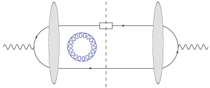
Figure 8: Diagrammatic representation of the divergent part of virtual contributions. The blue gluon loop represents a generic divergence (UV or IR).

Starting from Ref. Boussarie:2016ogo , the divergent part of the one-loop cross-section, symbolically illustrated in Fig. 8 can be written as

$$\frac{d\hat{\sigma}_{1JI}}{dx_{q}d^{d}\vec{p}_{q}}=\frac{\alpha_{s}}{2\pi}\frac{\Gamma(1-\epsilon)}{(4\pi)^{\epsilon}}C_{F}\left(\frac{S_{V}+S_{V}^{*}}{2}\right)\frac{d\hat{\sigma}_{0LL}}{dx_{q}d^{d}\vec{p}_{q}}\;,$$ (53)

where

$$\frac{S_{V}+S_{V}^{*}}{2}=\frac{1}{\epsilon}\Bigg{[}-4\epsilon\ln(\alpha)\ln\left(\frac{x_{q}^{2}x_{\bar{q}}^{2}\mu^{2}}{\left(x_{q}\vec{p}_{\bar{q}}-x_{\bar{q}}\vec{p}_{q}\right)^{2}}\right)+4\ln(\alpha)+4\epsilon\ln^{2}(\alpha)-2\ln(x_{q}x_{\bar{q}})+3$$

$$+2\epsilon\ln\left(\frac{x_{q}x_{\bar{q}}\mu^{2}}{\left(x_{q}\vec{p}_{\bar{q}}-x_{\bar{q}}\vec{p}_{q}\right)^{2}}\right)\ln(x_{q}x_{\bar{q}})+\epsilon\ln^{2}(x_{q}x_{\bar{q}})-3\epsilon\ln\left(\frac{x_{q}x_{\bar{q}}\mu^{2}}{\left(x_{q}\vec{p}_{\bar{q}}-x_{\bar{q}}\vec{p}_{q}\right)^{2}}\right)-\frac{\pi^{2}}{3}\epsilon+6\epsilon\Bigg{]}\,.$$ (54)

Performing the convolution with FFs as in (19) and using (21), we can get the final contribution separated into a divergent and a finite part, i.e.

$$\frac{d\sigma_{JI}^{q\rightarrow h}}{dx_{h}d^{d}p_{h\perp}}\bigg{|}_{S_{V}}=\frac{2\alpha_{\mathrm{em}}Q^{2}}{(2\pi)^{4d}N_{c}\;x_{h}^{d}}\sum_{q}Q_{q}^{2}\int_{x_{h}}^{1}dx_{q}\;x_{q}^{1+d}(1-x_{q})^{2}\int d^{d}p_{\bar{q}\perp}\int d^{d}p_{2\perp}\int d^{d}p_{2^{\prime}\perp}$$

$$\times\frac{\mathbf{F}\left(\frac{x_{q}}{2x_{h}}p_{h\perp}+\frac{1}{2}p_{\bar{q}\perp}-p_{2\perp}\right)}{\vec{p}_{\bar{q}2}^{\;2}+x_{q}(1-x_{q})Q^{2}}\;\frac{\mathbf{F}^{*}\left(\frac{x_{q}}{2x_{h}}p_{h\perp}+\frac{1}{2}p_{\bar{q}\perp}-p_{2^{\prime}\perp}\right)}{\vec{p}_{\bar{q}2^{\prime}}^{\;2}+x_{q}(1-x_{q})Q^{2}}D_{q}^{h}\left(\frac{x_{h}}{x_{q}},\mu_{F}\right)\delta_{JI}$$

$$\times\frac{\alpha_{s}}{2\pi}C_{F}\left(\frac{1}{\hat{\epsilon}}A_{V,\text{div}}+A_{V,\text{fin}}\right)\equiv\frac{d\sigma_{JI}^{q\rightarrow h}}{dx_{h}d^{d}p_{h\perp}}\bigg{|}_{S_{V}\text{,div}}+\frac{d\sigma_{JI}^{q\rightarrow h}}{dx_{h}d^{d}p_{h\perp}}\bigg{|}_{S_{V}\text{,fin}}\;,$$ (55)

where

$$A_{V,\text{div}}=4\ln\alpha-2\ln x_{q}(1-x_{q})+3-4\epsilon\ln\alpha\ln\left(\frac{x_{h}^{2}(1-x_{q})^{2}\mu^{2}}{\left(x_{h}\vec{p}_{\bar{q}}-(1-x_{q})\vec{p}_{h}\right)^{2}}\right)+\epsilon\ln^{2}\alpha^{2}\;,$$ (56)

$$A_{V,\text{fin}}=\left(2\ln x_{q}(1-x_{q})-3\right)\ln\left(\frac{x_{h}^{2}(1-x_{q})\mu^{2}}{x_{q}\left(x_{h}\vec{p}_{\bar{q}}-(1-x_{q})\vec{p}_{h}\right)^{2}}\right)$$

$$+2\left(3-\zeta(2)+\frac{1}{2}\ln^{2}(x_{q}(1-x_{q}))\right)$$ (57)

and

$$\delta_{LL}=1\;,\hskip 28.45274pt\delta_{TL}=\frac{(1-2x_{q})}{2x_{q}(1-x_{q})Q}\left(\vec{p}_{\bar{q}2^{\prime}}\cdot\vec{\varepsilon}_{T}\right)^{*}\;,$$

$$\delta_{TT}=\left[(1-2x_{q})^{2}g_{\perp}^{ri}g_{\perp}^{lk}-g_{\perp}^{rk}g_{\perp}^{li}+g_{\perp}^{rl}g_{\perp}^{ik}\right]\frac{\varepsilon_{Ti}\;p_{\bar{q}2\perp r}\left(\varepsilon_{Tk}\;p_{\bar{q}2^{\prime}\perp l}\right)^{*}}{4x_{q}^{2}(1-x_{q})^{2}Q^{2}}\;.$$ (58)

Again, the corresponding contribution in the case of fragmentation from anti-quark is obtained by including a minus sign in the argument of the function F, extending the sum over $q$ to the five anti-quark flavor species and performing the $(q\leftrightarrow\bar{q})$ relabelling (also inside the functions $A_{V,{\rm{div}}}$, $A_{V,{\rm{fin}}}$, $\delta_{JI}$).

4.2 Finite part of the dipole $\times$ dipole contribution

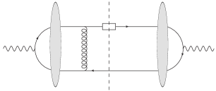
Figure 9: An example of diagram which only contributes to the dipole $\times$ dipole part of virtual contributions.

An example of diagram contributing to the dipole $\times$ dipole part is shown in Fig. 9. Let us now consider the finite part associated with these diagrams. This contribution reads

$$\frac{d\sigma_{LL}^{q\rightarrow h}}{dx_{h}d^{2}p_{h\perp}}\bigg{|}_{\text{virt., dip. $\times$ dip.}}=\frac{2\alpha_{\mathrm{em}}Q^{2}}{\left(2\pi\right)^{8}N_{c}\;x_{h}^{2}}\sum_{q}Q_{q}^{2}\int_{x_{h}}^{1}dx_{q}x_{q}D_{q}^{h}\left(\frac{x_{h}}{x_{q}},\mu_{F}\right)\frac{\alpha_{s}}{2\pi}\frac{C_{F}}{4}$$

$$\times\int d^{2}\vec{p}_{\bar{q}}d^{2}\vec{p}_{1}d^{2}\vec{p}_{2}d^{2}\vec{p}_{1^{\prime}}d^{2}\vec{p}_{2^{\prime}}\delta\left(\frac{x_{q}}{x_{h}}\vec{p}_{h}-\vec{p}_{1}+\vec{p}_{\bar{q}2}\right)\delta(\vec{p}_{11^{\prime}}+\vec{p}_{22^{\prime}})\mathbf{F}\left(\frac{\vec{p}_{12}}{2}\right)\mathbf{F}^{\ast}\left(\frac{\vec{p}_{1^{\prime}2^{\prime}}}{2}\right)$$

$$\times\left\{\frac{1}{{\vec{p}_{q1^{\prime}}^{\;2}+x_{q}x_{\bar{q}}Q^{2}}}\left[\frac{6x_{q}^{2}x_{\bar{q}}^{2}}{\vec{p}_{q1}^{\;2}+x_{q}x_{\bar{q}}Q^{2}}\ln\left(\frac{x_{q}^{2}x_{\bar{q}}^{2}\mu^{4}Q^{2}}{(x_{q}\vec{p}_{\bar{q}}-x_{\bar{q}}\vec{p}_{q})^{2}(\vec{p}_{q1}^{\;2}+x_{q}x_{\bar{q}}Q^{2})^{2}}\right)\right.\right.$$

$$\left.\left.+\left(\int_{0}^{x_{q}}dz\left(\left[(\phi_{4})_{LL}\right]_{+}+\sum_{n=5,6}\left[(\phi_{n})_{LL}\right]_{+}|_{\vec{p}_{3}=\vec{0}}\right)+(q\leftrightarrow\bar{q})\right)\right]+h.c.|_{p_{1},p_{2}\leftrightarrow p_{1^{\prime}},p_{2^{\prime}}}\right\}_{\begin{subarray}{c}x_{\bar{q}}=1-x_{q}\\ \vec{p}_{q}=\frac{x_{q}}{x_{h}}\vec{p}_{h}\end{subarray}},$$ (59)

in the LL case,

$$\frac{d\sigma_{TL}^{q\rightarrow h}}{dx_{h}d^{2}p_{h\perp}}\bigg{|}_{\text{virt., dip. $\times$ dip.}}=\frac{\alpha_{\mathrm{em}}Q}{(2\pi)^{8}N_{c}\;x_{h}^{2}}\sum_{q}Q_{q}^{2}\int_{x_{h}}^{1}dx_{q}x_{q}D_{q}^{h}\left(\frac{x_{h}}{x_{q}},\mu_{F}\right)\frac{\alpha_{s}}{4\pi}C_{F}\varepsilon_{Ti}^{\ast}$$

$$\times\int d^{2}\vec{p}_{\bar{q}}d^{2}\vec{p}_{1}d^{2}\vec{p}_{2}d^{2}\vec{p}_{1^{\prime}}d^{2}\vec{p}_{2^{\prime}}\delta\left(\frac{x_{q}}{x_{h}}\vec{p}_{h}-\vec{p}_{1}+\vec{p}_{\bar{q}2}\right)\delta(\vec{p}_{11^{\prime}}+\vec{p}_{22^{\prime}})\mathbf{F}\left(\frac{\vec{p}_{12\bot}}{2}\right)\mathbf{F}^{\ast}\left(\frac{\vec{p}_{1^{\prime}2^{\prime}}}{2}\right)$$

$$\times\left\{\frac{\displaystyle\left[\left(\int_{0}^{x_{q}}dz\left(\left[(\phi_{4})^{i}_{TL}\right]_{+}+\sum\limits_{n=5,6}\left[(\phi_{n})^{i}_{TL}\right]_{+}|_{\vec{p}_{3}=\vec{0}}\right)\right)+(q\leftrightarrow\bar{q})\right]^{\ast}}{\vec{p}_{q1}^{\;2}+x_{q}x_{\bar{q}}Q^{2}}+\frac{3x_{q}x_{\bar{q}}(1-2x_{q})p_{q1^{\prime}\bot}^{i}}{(\vec{p}_{q1}^{\;2}+x_{q}x_{\bar{q}}Q^{2})}\right.$$

$$\times\frac{1}{(\vec{p}_{q1^{\prime}}^{\;2}+x_{q}x_{\bar{q}}Q^{2})}\left(\ln\left(\frac{x_{q}^{3}x_{\bar{q}}^{3}\mu^{8}Q^{2}(x_{q}\vec{p}_{\bar{q}}-x_{\bar{q}}\vec{p}_{q})^{-4}}{(\vec{p}_{q1}^{\;2}+x_{q}x_{\bar{q}}Q^{2})^{2}(\vec{p}_{q1^{\prime}}^{\;2}+x_{q}x_{\bar{q}}Q^{2})}\right)\right.-\left.\frac{x_{q}x_{\bar{q}}Q^{2}}{\vec{p}_{q1^{\prime}}^{\;2}}\ln\left(\frac{x_{q}x_{\bar{q}}Q^{2}}{\vec{p}_{q1^{\prime}}^{\;2}+x_{q}x_{\bar{q}}Q^{2}}\right)\right)$$

$$+\left.\frac{\displaystyle\left[\left(\int_{0}^{x_{q}}dz\left(\left[(\phi_{4})_{LT}^{i}\right]_{+}+\sum\limits_{n=5,6}\left[(\phi_{n})_{LT}^{i}\right]_{+}|_{\vec{p}_{3}=\vec{0}}\right)\right)+\left(q\leftrightarrow\bar{q}\right)\right]}{2x_{q}x_{\bar{q}}\left(\vec{p}_{q1^{\prime}}^{\;2}+x_{q}x_{\bar{q}}Q^{2}\right)}\right\}_{\begin{subarray}{c}x_{\bar{q}}=1-x_{q}\\ \vec{p}_{q}=\frac{x_{q}}{x_{h}}\vec{p}_{h}\end{subarray}}\;,$$ (60)

in the TL case, and

$$\frac{d\sigma_{TT}^{q\rightarrow h}}{dx_{h}d^{2}p_{h\perp}}\bigg{|}_{\text{virt., dip. $\times$ dip.}}=\frac{\alpha_{\mathrm{em}}}{2\left(2\pi\right)^{8}N_{c}\;x_{h}^{2}}\sum_{q}Q_{q}^{2}\int_{x_{h}}^{1}dx_{q}x_{q}D_{q}^{h}\left(\frac{x_{h}}{x_{q}},\mu_{F}\right)(\varepsilon_{Ti}\varepsilon_{Tk}^{\ast})$$

$$\times\int d^{2}\vec{p}_{\bar{q}}d^{2}\vec{p}_{1}d^{d}\vec{p}_{2}d^{2}\vec{p}_{1^{\prime}}d^{2}\vec{p}_{2^{\prime}}\delta\left(\frac{x_{q}}{x_{h}}\vec{p}_{h}-\vec{p}_{1}+\vec{p}_{\bar{q}2}\right)\delta(\vec{p}_{11^{\prime}}+\vec{p}_{22^{\prime}})\mathbf{F}\left(\frac{\vec{p}_{12}}{2}\right)\mathbf{F}^{\ast}\left(\frac{\vec{p}_{1^{\prime}2^{\prime}}}{2}\right)$$

$$\times\frac{\alpha_{s}}{2\pi}C_{F}\Bigg{\{}\frac{3}{2}\frac{p_{q1\bot r}p_{q1^{\prime}\bot l}}{(\vec{p}_{q1}^{\;2}+x_{q}x_{\bar{q}}Q^{2})(\vec{p}_{q1^{\prime}}^{\;2}+x_{q}x_{\bar{q}}Q^{2})}\left[(1-2x_{q})^{2}g_{\bot}^{ri}g_{\bot}^{lk}-g_{\bot}^{rk}g_{\bot}^{li}+g_{\bot}^{rl}g_{\bot}^{ik}\right]$$

$$\times\left[\ln\left(\frac{x_{q}x_{\bar{q}}\mu^{4}}{(x_{q}\vec{p}_{\bar{q}}-x_{\bar{q}}\vec{p}_{q})^{2}(\vec{p}_{q1}^{\;2}+x_{q}x_{\bar{q}}Q^{2})}\right)-\frac{x_{q}x_{\bar{q}}Q^{2}}{\vec{p}_{q1}^{\;2}}\ln\left(\frac{x_{q}x_{\bar{q}}Q^{2}}{\vec{p}_{q1}^{\;2}+x_{q}x_{\bar{q}}Q^{2}}\right)\right]$$

$$+\left.\frac{\displaystyle\left[\left(\int_{0}^{x_{q}}dz\left(\left[(\phi_{4})^{ik}_{TT}\right]_{+}+\sum\limits_{n=5,6}\left[(\phi_{n})^{ik}_{TT}\right]_{+}|_{\vec{p}_{3}=\vec{0}}\right)\right)+\left(q\leftrightarrow\bar{q}\right)\right]}{x_{q}x_{\bar{q}}\left(\vec{p}_{q1^{\prime}}^{\,\,2}+x\bar{x}Q^{2}\right)}+h.c.|_{\begin{subarray}{c}p_{1},p_{2}\leftrightarrow p_{1^{\prime}},p_{2^{\prime}}\\ i\leftrightarrow k\end{subarray}}\right\}_{\begin{subarray}{c}x_{\bar{q}}=1-x_{q}\\ \vec{p}_{q}=\frac{x_{q}}{x_{h}}\vec{p}_{h}\end{subarray}}\;,$$ (61)

in the TT case. The explicit expression for the functions $(\phi_{n})_{JI}$ can be found in appendix B.

4.3 Dipole $\times$ double dipole contribution

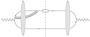
Figure 10: An example of diagram which contributes to the dipole $\times$ double dipole part of virtual contributions.

In the dipole $\times$ double dipole contribution, the virtual gluon crosses the shockwave (see Fig. 10). This contribution, after the subtraction of rapidity divergences, reads

$$\frac{d\sigma_{LL}^{q\rightarrow h}}{dx_{h}d^{2}p_{h\perp}}\bigg{|}_{\text{virt., dip. $\times$ d. dip.}}=\frac{2\alpha_{\mathrm{em}}Q^{2}}{\left(2\pi\right)^{8}N_{c}\,x_{h}^{2}}\sum_{q}Q_{q}^{2}\int_{x_{h}}^{1}dx_{q}x_{q}D_{q}^{h}\left(\frac{x_{h}}{x_{q}},\mu_{F}\right)\int d^{2}\vec{p}_{\bar{q}}d^{2}\vec{p}_{1}d^{2}\vec{p}_{2}d^{2}\vec{p}_{1^{\prime}}d^{2}\vec{p}_{2^{\prime}}$$

$$\times\int\frac{d^{2}\vec{p}_{3}}{\left(2\pi\right)^{2}}\delta\left(\frac{x_{q}}{x_{h}}\vec{p}_{h}-\vec{p}_{1}+\vec{p}_{\bar{q}2}-\vec{p}_{3}\right)\delta(\vec{p}_{11^{\prime}}+\vec{p}_{22^{\prime}}+\vec{p}_{3})\frac{\alpha_{s}}{2\pi}\frac{1}{8}\left\{\frac{1}{\vec{p}_{q1^{\prime}}^{\;2}+x_{q}x_{\bar{q}}Q^{2}}\widetilde{\mathbf{F}}\left(\frac{\vec{p}_{12}}{2},\vec{p}_{3}\right)\right.$$

$$\times\mathbf{F}^{\ast}\left(\frac{\vec{p}_{1^{\prime}2^{\prime}}}{2}\right)\left[4x_{q}x_{\bar{q}}\left[\frac{x_{q}x_{\bar{q}}(\vec{p}_{3}^{\;2}-\vec{p}_{\bar{q}2}^{\;2}-\vec{p}_{q1}^{\;2}-2x_{q}x_{\bar{q}}Q^{2})}{(\vec{p}_{\bar{q}2}^{\;2}+x_{q}x_{\bar{q}}Q^{2})(\vec{p}_{q1}^{\;2}+x_{q}x_{\bar{q}}Q^{2})-x_{q}x_{\bar{q}}Q^{2}\vec{p}_{3}^{\;2}}\ln\left(\frac{x_{q}x_{\bar{q}}}{e^{2\eta}}\right)\right.\right.$$

$$\times\ln\left(\frac{(\vec{p}_{\bar{q}2}^{\;2}+x_{q}x_{\bar{q}}Q^{2})\left(\vec{p}_{q1}^{\;2}+x_{q}x_{\bar{q}}Q^{2}\right)}{x_{q}x_{\bar{q}}Q^{2}\vec{p}_{3}^{\;2}}\right)-\left.\left(\frac{2x_{q}x_{\bar{q}}}{\vec{p}_{q1}^{\;2}+x_{q}x_{\bar{q}}Q^{2}}\ln\left(\frac{x_{\bar{q}}}{e^{\eta}}\right)\ln\left(\frac{\vec{p}_{3}^{\;2}}{\mu^{2}}\right)+\left(q\leftrightarrow\bar{q}\right)\right)\right]$$

$$+\left.\left.Q^{2}\left[\left(\int_{0}^{x_{q}}dz\sum_{n=5,6}\left[(\phi_{n})_{LL}\right]_{+}\right)+\left(q\leftrightarrow\bar{q}\right)\right]\right]+h.c.|_{p_{1},p_{1}\leftrightarrow p_{1^{\prime}},p_{2^{\prime}}}\right\}_{\begin{subarray}{c}x_{\bar{q}}=1-x_{q}\\ \vec{p}_{q}=\frac{x_{q}}{x_{h}}\vec{p}_{h}\end{subarray}}\;,$$ (62)

in the LL case,

$$\frac{d\sigma_{TL}^{q\rightarrow h}}{dx_{h}d^{2}p_{h\perp}}\bigg{|}_{\text{virt., dip. $\times$ d. dip.}}=\frac{\alpha_{\mathrm{em}}Q}{\left(2\pi\right)^{8}N_{c}\,x_{h}^{2}}\sum_{q}Q_{q}^{2}\int_{x_{h}}^{1}dx_{q}x_{q}D_{q}^{h}\left(\frac{x_{h}}{x_{q}},\mu_{F}\right)\int d^{2}\vec{p}_{\bar{q}}d^{2}\vec{p}_{1}d^{2}\vec{p}_{2}d^{2}\vec{p}_{1^{\prime}}d^{2}\vec{p}_{2^{\prime}}$$

$$\times\int\frac{d^{2}\vec{p}_{3}d^{2}\vec{p}_{3^{\prime}}}{(2\pi)^{2}}\delta\left(\frac{x_{q}}{x_{h}}\vec{p}_{h}-\vec{p}_{1}+\vec{p}_{\bar{q}2}-\vec{p}_{3}\right)\delta(\vec{p}_{11^{\prime}}+\vec{p}_{22^{\prime}}+\vec{p}_{33^{\prime}})\frac{\alpha_{s}}{8\pi}\varepsilon_{Ti}^{\ast}\left\{\frac{\delta(\vec{p}_{3^{\prime}})}{\vec{p}_{q1^{\prime}}^{\;2}+x_{q}x_{\bar{q}}Q^{2}}\widetilde{\mathbf{F}}\left(\frac{\vec{p}_{12}}{2},\vec{p}_{3}\right)\right.$$

$$\times\mathbf{F}^{\ast}\left(\frac{\vec{p}_{1^{\prime}2^{\prime}}}{2}\right)\left[2(1-2x_{q})p_{q1^{\prime}\bot}^{i}\left[\frac{x_{q}x_{\bar{q}}(\vec{p}_{3}^{\;2}-\vec{p}_{\bar{q}2}^{\;2}-\vec{p}_{q1}^{\;2}-2x_{q}x_{\bar{q}}Q^{2})}{(\vec{p}_{\bar{q}2}^{\;2}+x_{q}x_{\bar{q}}Q^{2})(\vec{p}_{q1}^{\;2}+x_{q}x_{\bar{q}}Q^{2})-x_{q}x_{\bar{q}}Q^{2}\vec{p}_{3}^{\;2}}\right.\right.\ln\left(\frac{x_{q}x_{\bar{q}}}{e^{2\eta}}\right)$$

$$\times\ln\left(\frac{(\vec{p}_{\bar{q}2}^{\;2}+x_{q}x_{\bar{q}}Q^{2})\left(\vec{p}_{q1}^{\;2}+x_{q}x_{\bar{q}}Q^{2}\right)}{x_{q}x_{\bar{q}}Q^{2}\vec{p}_{3}^{\;2}}\right)-\left.\left(\frac{2x_{q}x_{\bar{q}}}{\vec{p}_{q1}^{\;2}+x_{q}x_{\bar{q}}Q^{2}}\ln\left(\frac{x_{\bar{q}}}{e^{\eta}}\right)\ln\left(\frac{\vec{p}_{3}^{\;2}}{\mu^{2}}\right)+\left(q\leftrightarrow\bar{q}\right)\right)\right]$$

$$+\left.\frac{1}{2x_{q}x_{\bar{q}}}\left[\left(\int_{0}^{x_{q}}dz\sum_{n=5,6}\left[(\phi_{n})^{i}_{TL}\right]_{+}\right)+\left(q\leftrightarrow\bar{q}\right)\right]\right]+\frac{\delta(\vec{p}_{3})}{\vec{p}_{q1}^{\;2}+x_{q}x_{\bar{q}}Q^{2}}\widetilde{\mathbf{F}}^{\ast}\left(\frac{\vec{p}_{1^{\prime}2^{\prime}}}{2},\vec{p}_{3^{\prime}}\right)$$

$$\times\mathbf{F}\left(\frac{\vec{p}_{12}}{2}\right)\left[\left[2x_{q}x_{\bar{q}}(1-2x_{q})p_{q1^{\prime}\bot}^{i}\left(\frac{-2}{\vec{p}_{q1^{\prime}}^{\;2}+x_{q}x_{\bar{q}}Q^{2}}\ln\left(\frac{x_{\bar{q}}}{e^{\eta}}\right)\ln\left(\frac{\vec{p}_{3^{\prime}}^{\;2}}{\mu^{2}}\right)+\ln\left(\frac{x_{q}x_{\bar{q}}}{e^{2\eta}}\right)\right.\right.\right.$$

$$\times\left(\frac{-(\vec{p}_{\bar{q}2^{\prime}}^{\;2}+x_{q}x_{\bar{q}}Q^{2})}{(\vec{p}_{q1^{\prime}}^{\;2}+x_{q}x_{\bar{q}}Q^{2})(\vec{p}_{\bar{q}2^{\prime}}^{\;2}+x_{q}x_{\bar{q}}Q^{2})-x_{q}x_{\bar{q}}Q^{2}\vec{p}_{3^{\prime}}^{\;2}}\right.\ln\left(\frac{(\vec{p}_{q1^{\prime}}^{\;2}+x_{q}x_{\bar{q}}Q^{2})(\vec{p}_{\bar{q}2^{\prime}}^{\;2}+x_{q}x_{\bar{q}}Q^{2})}{x_{q}x_{\bar{q}}Q^{2}\vec{p}_{3^{\prime}}^{\;2}}\right)$$

$$+\left.\left.\left.\frac{1}{\vec{p}_{q1^{\prime}}^{\;2}}\ln\left(\frac{\vec{p}_{q1^{\prime}}^{\;2}+x_{q}x_{\bar{q}}Q^{2}}{x_{q}x_{\bar{q}}Q^{2}}\right)\right)\right)+(q\leftrightarrow\bar{q})\right]+\left.\left.\left[\left(\int_{0}^{x_{q}}dz\sum_{n=5,6}\left[(\phi_{n})_{LT}^{i}\right]_{+}\right)+\left(q\leftrightarrow\bar{q}\right)\right]^{\ast}\right]\right\}_{\begin{subarray}{c}x_{\bar{q}}=1-x_{q}\\ \vec{p}_{q}=\frac{x_{q}}{x_{h}}\vec{p}_{h}\end{subarray}}\;$$ (63)

in the TL case, and

$$\frac{d\sigma_{TT}^{q\rightarrow h}}{dx_{h}d^{2}p_{h\perp}}\bigg{|}_{\text{virt., dip. $\times$ d. dip.}}=\frac{\alpha_{\mathrm{em}}}{2\left(2\pi\right)^{8}N_{c}\,x_{h}^{2}}\sum_{q}Q_{q}^{2}\int_{x_{h}}^{1}dx_{q}x_{q}D_{q}^{h}\left(\frac{x_{h}}{x_{q}},\mu_{F}\right)\int\,d^{2}\vec{p}_{1}\,d^{2}\vec{p}_{2}\,d^{2}\vec{p}_{1^{\prime}}\,d^{2}\vec{p}_{2^{\prime}}$$

$$\times\int d^{2}\vec{p}_{\bar{q}}\int\frac{d^{2}\vec{p}_{3}}{\left(2\pi\right)^{2}}\delta\left(\frac{x_{q}}{x_{h}}\vec{p}_{h}-\vec{p}_{1}+\vec{p}_{\bar{q}2}-\vec{p}_{3}\right)\delta(\vec{p}_{11^{\prime}}+\vec{p}_{22^{\prime}}+\vec{p}_{3})\frac{\alpha_{s}}{4\pi}(\varepsilon_{Ti}\varepsilon_{Tj}^{\ast})\Bigg{\{}\widetilde{\mathbf{F}}\left(\frac{\vec{p}_{12}}{2},\vec{p}_{3}\right)\mathbf{F}^{\ast}\left(\frac{\vec{p}_{1^{\prime}2^{\prime}}}{2}\right)$$

$$\times\frac{1}{\vec{p}_{q1^{\prime}}^{\,\,2}+x_{q}x_{\bar{q}}Q^{2}}\left[\left[p_{q1^{\prime}\bot l}p_{q1\bot k}\left[(1-2x)^{2}g_{\bot}^{ki}g_{\bot}^{lj}-g_{\bot}^{kj}g_{\bot}^{li}+g_{\bot}^{kl}g_{\bot}^{ij}\right]\left[\frac{\displaystyle-2\ln\left(\frac{x_{\bar{q}}}{e^{\eta}}\right)\ln\left(\frac{\vec{p}_{3}^{\;2}}{\mu^{2}}\right)}{\vec{p}_{q1}^{\;2}+x_{q}x_{\bar{q}}Q^{2}}\right.\right.\right.$$

$$+\ln\left(\frac{x_{q}x_{\bar{q}}}{e^{2\eta}}\right)\left(\frac{1}{\vec{p}_{q1}^{\;2}}\ln\left(\frac{\vec{p}_{q1}^{\;2}+x_{q}x_{\bar{q}}Q^{2}}{x_{q}x_{\bar{q}}Q^{2}}\right)\right.-\frac{\vec{p}_{\bar{q}2}^{\;2}+x_{q}x_{\bar{q}}Q^{2}}{(\vec{p}_{q1}^{\;2}+x_{q}x_{\bar{q}}Q^{2})(\vec{p}_{\bar{q}2}^{\;2}+x_{q}x_{\bar{q}}Q^{2})-x_{q}x_{\bar{q}}Q^{2}\vec{p}_{3}^{\;2}}$$

$$\times\left.\left.\left.\ln\left(\frac{(\vec{p}_{q1}^{\;2}+x_{q}x_{\bar{q}}Q^{2})(\vec{p}_{\bar{q}2}^{\;2}+x_{q}x_{\bar{q}}Q^{2})}{x_{q}x_{\bar{q}}Q^{2}\vec{p}_{3}^{\;2}}\right)\right)\right]+(q\leftrightarrow\bar{q})\right]$$

$$+\left.\frac{1}{x_{q}x_{\bar{q}}}\left[\left(\int_{0}^{x_{q}}dz\sum_{n=5,6}\left[(\phi_{n})^{ij}_{TT}\right]_{+}\right)+\left(q\leftrightarrow\bar{q}\right)\right]\right]+h.c.|_{\begin{subarray}{c}p_{1},p_{2}\leftrightarrow p_{1^{\prime}},p_{2^{\prime}}\\ i\leftrightarrow j\end{subarray}}\Bigg{\}}_{\begin{subarray}{c}x_{\bar{q}}=1-x_{q}\\ \vec{p}_{q}=\frac{x_{q}}{x_{h}}\vec{p}_{h}\end{subarray}}\;,$$ (64)

in the TT case.

The corresponding finite virtual contributions in the case of anti-quark fragmentation are obtained as follows: 1) by changing the integration variables $x_{q},\vec{p}_{\bar{q}}$ to $x_{\bar{q}},\vec{p}_{q}$, 2) extending the sum over $q$ to anti-quark flavor types (in order to have the FFs of anti-quarks), 3) computing the objects in the curly brackets fixing $x_{q}=1-x_{\bar{q}}$ and $\vec{p}_{\bar{q}}=\frac{x_{\bar{q}}}{x_{h}}\vec{p}_{h}$ and 4) making the changes $x_{q}\rightarrow x_{\bar{q}}$ and $\vec{p}_{\bar{q}}\rightarrow\vec{p}_{q}$ in the argument of the first delta function.

5 NLO cross-section: Divergent part of real corrections

5.1 Divergent part of the dipole $\times$ dipole cross-section

The dipole-dipole partonic cross-section is given by Eq. (6.6) of Ref. Boussarie:2016ogo :

$$d\hat{\sigma}_{3JI}=\frac{\alpha_{s}}{\mu^{2\epsilon}}\left(\frac{N_{c}^{2}-1}{N_{c}}\right)\frac{\alpha_{\mathrm{em}}Q_{q}^{2}}{2(2\pi)^{4d}N_{c}}\frac{(p_{0}^{-})^{2}}{s^{2}x_{q}^{\prime}x_{\bar{q}}^{\prime}}\varepsilon_{I\alpha}\varepsilon_{J\beta}^{*}dx_{q}^{\prime}dx_{\bar{q}}^{\prime}\delta(1-x_{q}^{\prime}-x_{\bar{q}}^{\prime}-x_{g})d^{d}p_{q\perp}d^{d}p_{\bar{q}\perp}$$

$$\times\frac{dx_{g}d^{d}p_{g\perp}}{x_{g}(2\pi)^{d}}\int d^{d}p_{1\perp}d^{d}p_{2\perp}\mathbf{F}\left(\frac{p_{12\perp}}{2}\right)\delta(p_{q1\perp}+p_{\bar{q}2\perp}+p_{g\perp})\int d^{d}p_{1^{\prime}\perp}d^{d}p_{2^{\prime}\perp}\mathbf{F}^{*}\left(\frac{p_{1^{\prime}2^{\prime}\perp}}{2}\right)$$

$$\times\delta(p_{q1^{\prime}\perp}+p_{\bar{q}2^{\prime}\perp}+p_{g\perp})\Phi_{3}^{\alpha}(p_{1\perp},p_{2\perp})\Phi_{3}^{\beta*}(p_{1^{\prime}\perp},p_{2^{\prime}\perp})\;.$$ (65)

where we introduce shorthand notation by suppressing summation over helicities of partons

$$\Phi_{3}^{\alpha}(p_{1\perp},p_{2\perp})\Phi_{3}^{\beta*}(p_{1^{\prime}\perp},p_{2^{\prime}\perp})\equiv\sum_{\lambda_{q},\lambda_{g},\lambda_{\bar{q}}}\Phi_{3}^{\alpha}(p_{1\perp},p_{2\perp})\Phi_{3}^{\beta*}(p_{1^{\prime}\perp},p_{2^{\prime}\perp})\;.$$ (66)

For later convenience, we have also relabelled $x_{q}$ and $x_{\bar{q}}$ of Ref. Boussarie:2016ogo as $x_{q}^{\prime}$ and $x_{\bar{q}}^{\prime}$. This is because, in dealing with real contributions containing a $qg$ splitting (or even a $\bar{q}g$ splitting), we need to distinguish the longitudinal momentum fraction of the quark transported before and after the splitting.

The dipole part of the $\gamma^{(*)}\rightarrow q\bar{q}g$ impact factor has the form $\Phi_{3}^{\alpha}=\Phi_{4}^{\alpha}|_{\vec{p}_{3}=0}+\tilde{\Phi}_{3}^{\alpha}$, where $\tilde{\Phi}_{3}^{\alpha}$ is the contribution in which the gluon is emitted after the shockwave and $\Phi_{4}^{\alpha}$ is the contribution in which the gluon cross the shockwave with $\vec{p}_{3}$, the transverse momentum exchanged between the gluon and the shockwave, vanishes. Only the square of $\tilde{\Phi}_{3}^{\alpha}$ provides divergences in the cross-section and it is given by (B.3) in Ref. Boussarie:2016ogo .

The $LL$ contribution reads

$$\tilde{\Phi}_{3}^{+}(\vec{p}_{1},\vec{p}_{2})\tilde{\Phi}_{3}^{+*}(\vec{p}_{1^{\prime}},\vec{p}_{2^{\prime}})$$ (67)

$$=\frac{8x_{q}^{\prime}x_{\bar{q}}^{\prime}(p_{\gamma}^{+})^{4}\left(dx_{g}^{2}+4x_{q}^{\prime}(x_{q}^{\prime}+x_{g})\right)}{\left(Q^{2}+\frac{\vec{p}_{\bar{q}2}^{\,2}}{x_{\bar{q}}^{\prime}(1-x_{\bar{q}}^{\prime})}\right)\left(Q^{2}+\frac{\vec{p}_{\bar{q}2^{\prime}}^{\,2}}{x_{\bar{q}}^{\prime}(1-x_{\bar{q}}^{\prime})}\right)(x_{q}^{\prime}\vec{p}_{g}-x_{g}\vec{p}_{q})^{2}}$$

$$-\frac{8x_{q}^{\prime}x_{\bar{q}}^{\prime}(p_{\gamma}^{+})^{4}\left(2x_{g}-dx_{g}^{2}+4x_{q}^{\prime}x_{\bar{q}}^{\prime}\right)\left(x_{q}^{\prime}\vec{p}_{g}-x_{g}\vec{p}_{q}\right)\cdot\left(x_{\bar{q}}^{\prime}\vec{p}_{g}-x_{g}\vec{p}_{\bar{q}}\right)}{\left(Q^{2}+\frac{\vec{p}_{\bar{q}2^{\prime}}^{\,2}}{x_{\bar{q}}^{\prime}(1-x_{\bar{q}}^{\prime})}\right)\left(Q^{2}+\frac{\vec{p}_{q1}^{\,2}}{x_{q}^{\prime}(1-x_{q}^{\prime})}\right)\left(x_{q}^{\prime}\vec{p}_{g}-x_{g}\vec{p}_{q}\right)^{2}\left(x_{\bar{q}}^{\prime}\vec{p}_{g}-x_{g}\vec{p}_{\bar{q}}\right)^{2}}$$

$$+\frac{8x_{q}^{\prime}x_{\bar{q}}^{\prime}(p_{\gamma}^{+})^{4}\left(dx_{g}^{2}+4x_{\bar{q}}^{\prime}(x_{\bar{q}}^{\prime}+x_{g})\right)}{\left(Q^{2}+\frac{\vec{p}_{q1}^{\,2}}{x_{q}^{\prime}(1-x_{q}^{\prime})}\right)\left(Q^{2}+\frac{\vec{p}_{q1^{\prime}}^{\,2}}{x_{q}^{\prime}(1-x_{q}^{\prime})}\right)(x_{\bar{q}}^{\prime}\vec{p}_{g}-x_{g}\vec{p}_{\bar{q}})^{2}}$$

$$-\frac{8x_{q}^{\prime}x_{\bar{q}}^{\prime}(p_{\gamma}^{+})^{4}\left(2x_{g}-dx_{g}^{2}+4x_{q}^{\prime}x_{\bar{q}}^{\prime}\right)\left(x_{q}^{\prime}\vec{p}_{g}-x_{g}\vec{p}_{q}\right)\cdot\left(x_{\bar{q}}^{\prime}\vec{p}_{g}-x_{g}\vec{p}_{\bar{q}}\right)}{\left(Q^{2}+\frac{\vec{p}_{q1^{\prime}}^{\,2}}{x_{q}^{\prime}(1-x_{q}^{\prime})}\right)\left(Q^{2}+\frac{\vec{p}_{\bar{q}2}^{\,2}}{x_{\bar{q}}^{\prime}(1-x_{\bar{q}}^{\prime})}\right)\left(x_{q}^{\prime}\vec{p}_{g}-x_{g}\vec{p}_{q}\right)^{2}\left(x_{\bar{q}}^{\prime}\vec{p}_{g}-x_{g}\vec{p}_{\bar{q}}\right)^{2}}\,,$$

while, the $TL$ contribution is

$$\tilde{\Phi}_{3}^{+}(\vec{p}_{1},\vec{p}_{2})\tilde{\Phi}_{3}^{i*}(\vec{p}_{1^{\prime}},\vec{p}_{2^{\prime}})$$

$$=\frac{4x_{q}^{\prime}\left(p_{\gamma}^{+}\right)^{3}}{\left(x_{q}^{\prime}+x_{g}\right)\left(Q^{2}+\frac{\vec{p}_{\bar{q}2^{\prime}}^{\,2}}{x_{\bar{q}}^{\prime}\left(1-x_{\bar{q}}^{\prime}\right)}\right)\left(Q^{2}+\frac{\vec{p}_{q1}^{\,2}}{x_{q}^{\prime}\left(1-x_{q}^{\prime}\right)}\right)}\left(\frac{\left(x_{q}^{\prime}p_{g\perp}-x_{g}p_{q\perp}\right)_{\mu}\left(x_{\bar{q}}^{\prime}p_{g\perp}-x_{g}p_{\bar{q}\perp}\right)_{\nu}}{\left(x_{q}^{\prime}\vec{p}_{g}-x_{g}\vec{p}_{q}\right)^{2}\left(x_{\bar{q}}^{\prime}\vec{p}_{g}-x_{g}\vec{p}_{\bar{q}}\right)^{2}}\right)$$

$$\times\left[x_{g}\left(4x_{\bar{q}}^{\prime}+x_{g}d-2\right)\left(p_{\bar{q}2^{\prime}\perp}^{\mu}g_{\perp}^{i\nu}-p_{\bar{q}2^{\prime}\perp}^{\nu}g_{\perp}^{\mu i}\right)-\left(2x_{\bar{q}}^{\prime}-1\right)\left(4x_{q}^{\prime}x_{\bar{q}}^{\prime}+x_{g}\left(2-x_{g}d\right)\right)g_{\perp}^{\mu\nu}p_{\bar{q}2^{\prime}\perp}^{i}\right]$$

$$-\frac{4x_{q}^{\prime}\left(p_{\gamma}^{+}\right)^{3}\left(2x_{\bar{q}}^{\prime}-1\right)\left(x_{g}^{2}d+4x_{q}^{\prime}\left(x_{q}^{\prime}+x_{g}\right)\right)p_{\bar{q}2^{\prime}\perp}^{i}}{\left(x_{q}^{\prime}+x_{g}\right)\left(Q^{2}+\frac{\vec{p}_{\bar{q}2^{\prime}}^{\,2}}{x_{\bar{q}}^{\prime}\left(1-x_{\bar{q}}^{\prime}\right)}\right)\left(Q^{2}+\frac{\vec{p}_{\bar{q}2}^{\,2}}{x_{\bar{q}}^{\prime}\left(1-x_{\bar{q}}^{\prime}\right)}\right)\left(x_{q}^{\prime}\vec{p}_{g}-x_{g}\vec{p}_{q}\right)^{2}}+(q\leftrightarrow\bar{q})\,,$$ (68)

and, finally, the $TT$ contribution reads

$$\tilde{\Phi}_{3}^{i}(\vec{p}_{1},\vec{p}_{2})\tilde{\Phi}_{3}^{k*}(\vec{p}_{1^{\prime}},\vec{p}_{2^{\prime}})$$

$$=\frac{-2\left(p_{\gamma}^{+}\right)^{2}}{\left(x_{q}^{\prime}+x_{g}\right)\left(x_{\bar{q}}^{\prime}+x_{g}\right)\left(Q^{2}+\frac{\vec{p}_{\bar{q}2}^{\,2}}{x_{\bar{q}}^{\prime}\left(1-x_{\bar{q}}^{\prime}\right)}\right)\left(Q^{2}+\frac{\vec{p}_{q1^{\prime}}^{\,2}}{x_{q}^{\prime}\left(1-x_{q}^{\prime}\right)}\right)}$$

$$\times\left(\frac{\left(x_{q}^{\prime}p_{g\perp}-x_{g}p_{q\perp}\right)_{\mu}\left(x_{\bar{q}}^{\prime}p_{g\perp}-x_{g}p_{\bar{q}\perp}\right)_{\nu}}{\left(x_{q}^{\prime}\vec{p}_{g}-x_{g}\vec{p}_{q}\right)^{2}\left(x_{\bar{q}}^{\prime}\vec{p}_{g}-x_{g}\vec{p}_{\bar{q}}\right)^{2}}\right)\left\{x_{g}((d-4))x_{g}-2)\left[p_{q1^{\prime}\perp}^{\nu}\left(p_{\bar{q}2\perp}^{\mu}g_{\perp}^{ik}+p_{\bar{q}2\perp}^{k}g_{\perp}^{\mu i}\right)\right.\right.$$

$$\left.+g_{\perp}^{\mu\nu}\left(\left(\vec{p}_{q1^{\prime}}\cdot\vec{p}_{\bar{q}2}\right)g_{\perp}^{ik}+p_{q1^{\prime}\perp}^{i}p_{\bar{q}2\perp}^{k}\right)-g_{\perp}^{\nu k}p_{q1^{\prime}\perp}^{i}p_{\bar{q}2\perp}^{\mu}-g_{\perp}^{\mu i}g_{\perp}^{\nu k}\left(\vec{p}_{q1^{\prime}}\cdot\vec{p}_{\bar{q}2}\right)\right]-g_{\perp}^{\mu\nu}$$

$$\times\left[\left(2x_{q}^{\prime}-1\right)\left(2x_{\bar{q}}^{\prime}-1\right)p_{q1^{\prime}\perp}^{k}p_{\bar{q}2\perp}^{i}\left(4x_{q}^{\prime}x_{\bar{q}}^{\prime}+x_{g}(2-x_{g}d)\right)+4x_{q}^{\prime}x_{\bar{q}}^{\prime}((\vec{p}_{q1^{\prime}}\cdot\vec{p}_{\bar{q}2})g_{\perp}^{ik}+p_{q1^{\prime}\perp}^{i}p_{\bar{q}2\perp}^{k})\right]$$

$$+\left(p_{q1^{\prime}\perp}^{\mu}p_{\bar{q}2\perp}^{\nu}g_{\perp}^{ik}-p_{q1^{\prime}\perp}^{\mu}p_{\bar{q}2\perp}^{k}g_{\perp}^{\nu i}-p_{q1^{\prime}\perp}^{i}p_{\bar{q}2\perp}^{\nu}g_{\perp}^{\mu k}-g_{\perp}^{\mu k}g_{\perp}^{\nu i}(\vec{p}_{q1^{\prime}}\cdot\vec{p}_{\bar{q}2})\right)$$

$$\times x_{g}((d-4)x_{g}+2)+x_{g}(2x_{\bar{q}}^{\prime}-1)(x_{g}d+4x_{q}^{\prime}-2)\left(g_{\perp}^{\mu k}p_{q1^{\prime}\perp}^{\nu}-g_{\perp}^{\nu k}p_{q1^{\prime}\perp}^{\mu}\right)p_{\bar{q}2\perp}^{i}$$

$$\left.+x_{g}(2x_{q}^{\prime}-1)p_{q1^{\prime}\perp}^{k}(4x_{\bar{q}}^{\prime}+x_{g}d-2)\left(g_{\perp}^{\nu i}p_{\bar{q}2\perp}^{\mu}-g_{\perp}^{\mu i}p_{\bar{q}2\perp}^{\nu}\right)\right\}$$

$$-\frac{2x_{q}^{\prime}(p_{\gamma}^{+})^{2}(x_{g}^{2}d+4x_{q}^{\prime}(x_{q}^{\prime}+x_{g}))\left((\vec{p}_{\bar{q}2}\cdot\vec{p}_{\bar{q}2^{\prime}})g_{\perp}^{ik}-(1-2x_{\bar{q}}^{\prime})^{2}p_{\bar{q}2\perp}^{i}p_{\bar{q}2^{\prime}\perp}^{k}+p_{\bar{q}2^{\prime}\perp}^{i}p_{\bar{q}2\perp}^{k}\right)}{x_{\bar{q}}^{\prime}(x_{q}^{\prime}+x_{g})^{2}\left(Q^{2}+\frac{\vec{p}_{\bar{q}2}^{\,2}}{x_{\bar{q}}^{\prime}(1-x_{\bar{q}}^{\prime})}\right)\left(Q^{2}+\frac{\vec{p}_{\bar{q}2^{\prime}}^{\,2}}{x_{\bar{q}}^{\prime}(1-x_{\bar{q}}^{\prime})}\right)\left(x_{q}^{\prime}\vec{p}_{g}-x_{g}\vec{p}_{q}\right)^{2}}$$

$$+(q\leftrightarrow\bar{q})\,.$$ (69)

When two partons labeled $i$ and $j$ become collinear, the variable

$$\vec{A}_{ij}=x_{i}\vec{p}_{j}-x_{j}\vec{p}_{i}$$ (70)

vanishes. In the $LL$ case, for instance, the first term on the right-hand side of Eq. (67) gives the collinear divergence associated to the quark-gluon splitting ($\vec{A}_{qg}^{\;2}\to 0$), while the third gives the one associated to the anti-quark gluon splitting ($\vec{A}_{\bar{q}g}^{\;2}\to 0$).

The calculation technique of the divergent contributions is very similar for the different contributions afflicted by collinear divergences. For this reason, we present in the following sections the explicit extraction of the soft contribution and the explicit computation of one collinearly-divergent term. The others are obtained similarly.

5.2 Fragmentation from quark

In this section, we explicitly calculate the divergent contributions in the case of quark fragmentation. The evident symmetry with the case of anti-quarks allows us to provide the formulas for this second fragmentation mechanism as well.

5.2.1 Collinear contributions: $q$-$g$ splitting

Figure 11: The contribution containing the collinear-divergent part associated with the quark $\rightarrow$ quark $+$ gluon splitting, with the quark fragmenting into the identified hadronic state. The soft part (right diagram with the tiny red gluon) is subtracted from the total contribution (left diagram) in order to have the pure collinear divergence accompanied by finite terms.

The first contribution we calculate is shown in Fig. 11. The left-hand side diagram in Fig. 11 contains both soft and collinear divergences, as well as finite contributions. As mentioned before, soft contributions are treated separately, and therefore we subtract them from this contribution. The calculation of this contribution for the different cross sections $(LL,TL,TT)$ is practically identical, apart from the corrective factors, $\delta_{JI}$, which undergo trivial transformations but do not play any deep role. For simplicity of notation, we show the calculation in the $LL$ case and then give the final result in a completely general form valid for all different cases.

The term shown in Fig. 11 corresponds to the first term in Eq. (67). Performing the convolution as in Eq. (19) and using the explicit form of the hard cross-section in (65), we get

$$\frac{d\sigma_{LL}^{q\rightarrow h}}{dx_{h}d^{d}p_{h\perp}}\bigg{|}_{(1)}=\frac{\alpha_{s}C_{F}}{\mu^{2\epsilon}}\frac{2\alpha_{\mathrm{em}}Q^{2}}{(2\pi)^{4d}N_{c}}\sum_{q}Q_{q}^{2}\int_{x_{h}}^{1}\frac{dx_{q}^{\prime}}{x_{q}^{\prime}}D_{q}^{h}\left(\frac{x_{h}}{x_{q}^{\prime}},\mu_{F}\right)\left(\frac{x_{q}^{\prime}}{x_{h}}\right)^{d}\int d^{d}p_{\bar{q}\perp}$$

$$\times\int_{\alpha}^{1-x_{q}^{\prime}}\frac{dx_{g}}{x_{g}}\int\frac{d^{d}p_{g\perp}}{(2\pi)^{d}}\int d^{d}p_{1\perp}d^{d}p_{2\perp}\mathbf{F}\left(\frac{p_{12\perp}}{2}\right)\int d^{d}p_{1^{\prime}\perp}d^{d}p_{2^{\prime}\perp}\mathbf{F}^{*}\left(\frac{p_{1^{\prime}2^{\prime}\perp}}{2}\right)$$

$$\times\delta\left(\frac{x_{q}^{\prime}}{x_{h}}\vec{p}_{h}-p_{1\perp}+p_{\bar{q}2\perp}+p_{g\perp}\right)\delta\left(\frac{x_{q}^{\prime}}{x_{h}}\vec{p}_{h}-p_{1^{\prime}\perp}+p_{\bar{q}2^{\prime}\perp}+p_{g\perp}\right)$$

$$\times\frac{\left(dx_{g}^{2}+4x_{q}^{\prime}(x_{q}^{\prime}+x_{g})\right)(x_{q}^{\prime}+x_{g})^{2}(1-x_{q}^{\prime}-x_{g})^{2}}{(x_{q}^{\prime})^{2}\left((x_{q}^{\prime}+x_{g})(1-x_{q}^{\prime}-x_{g})Q^{2}+\vec{p}_{\bar{q}2}^{\,2}\right)\left((x_{q}^{\prime}+x_{g})(1-x_{q}^{\prime}-x_{g})Q^{2}+\vec{p}_{\bar{q}2^{\prime}}^{\,2}\right)\left(\vec{p}_{g}-\frac{x_{g}}{x_{h}}\vec{p}_{h}\right)^{2}}\;.$$ (71)

The cross section in Eq. (71) is expressed in terms of the fractions of longitudinal momenta of the initial photon carried by the quark and gluon produced after the splitting. However, to observe the cancellation of collinear divergences between this contribution and the counterterms coming from the renormalization of FF, it is necessary to perform the change of variables

$$x_{q}^{\prime}=\beta x_{q}\;,\hskip 14.22636ptx_{g}=(1-\beta)x_{q}\;,$$ (72)

where $x_{q}$ is the fraction of longitudinal momenta of the initial photon carried by the quark before the splitting, while $\beta$ is the fraction of longitudinal momenta of the initial quark carried by the final quark (see Fig. 12). Then, the longitudinal integrations become

$$\int_{x_{h}}^{1}dx_{q}^{\prime}\int_{\alpha}^{1-x_{q}^{\prime}}dx_{g}\;\;\big{[}.....\big{]}=\int_{x_{h}}^{1}dx_{q}\;x_{q}\int^{1-\frac{\alpha}{x_{q}}}_{\frac{x_{h}}{x_{q}}}d\beta\;\;\big{[}.....\big{]}_{\begin{subarray}{c}x_{g}=(1-\beta)x_{q}\\ x_{q}^{\prime}=\beta x_{q}\end{subarray}}\;,$$ (73)

where $\big{[}.....\big{]}$ represents the whole integrand function in Eq. (71) and the factor $x_{q}$ in the right hand side comes the Jacobian of the transformation in (72). After a bit of algebra, we end up with

Figure 12: Illustration of the change of variables in Eq. (72).

$$\frac{d\sigma_{LL}^{q\rightarrow h}}{dx_{h}d^{d}p_{h\perp}}\bigg{|}_{(1)}=\frac{2\alpha_{s}C_{F}}{\mu^{2\epsilon}}\frac{2\alpha_{\mathrm{em}}Q^{2}}{(2\pi)^{4d}N_{c}\,x_{h}^{d}}\sum_{q}Q_{q}^{2}\int_{x_{h}}^{1}dx_{q}\,x_{q}^{1+d}(1-x_{q})^{2}\int^{1-\frac{\alpha}{x_{q}}}_{\frac{x_{h}}{x_{q}}}\frac{d\beta}{\beta}$$

$$\times\frac{(1+\beta^{2}+\epsilon(1-\beta)^{2})}{\beta^{2-d}(1-\beta)}D_{q}^{h}\left(\frac{x_{h}}{\beta x_{q}},\mu_{F}\right)\int d^{d}p_{\bar{q}\perp}\int\frac{d^{d}p_{g\perp}}{(2\pi)^{d}}\int d^{d}p_{2\perp}\frac{\mathbf{F}\left(\frac{\beta x_{q}}{2x_{h}}\vec{p}_{h}+\frac{\vec{p}_{\bar{q}}}{2}+\frac{\vec{p}_{g}}{2}-\vec{p}_{2}\right)}{\left(x_{q}(1-x_{q})Q^{2}+\vec{p}_{\bar{q}2}^{\,2}\right)}$$

$$\times\int d^{d}p_{2^{\prime}\perp}\frac{\mathbf{F}^{*}\left(\frac{\beta x_{q}}{2x_{h}}\vec{p}_{h}+\frac{\vec{p}_{\bar{q}}}{2}+\frac{\vec{p}_{g}}{2}-\vec{p}_{2^{\prime}}\right)}{\left(x_{q}(1-x_{q})Q^{2}+\vec{p}_{\bar{q}2^{\prime}}^{\,2}\right)}\frac{1}{\left(\vec{p}_{g}-\frac{(1-\beta)x_{q}}{x_{h}}\vec{p}_{h}\right)^{2}}\,.$$ (74)

Then, it is convenient to express the functions $\mathbf{F},\mathbf{F}^{*}$ in terms of their Fourier transforms Eq. (16), i.e.

$$\mathbf{F}\left(\frac{\beta x_{q}}{2x_{h}}\vec{p}_{h}+\frac{\vec{p}_{\bar{q}}}{2}+\frac{\vec{p}_{g}}{2}-\vec{p}_{2}\right)=\int d^{d}\vec{z}_{1}\,F(\vec{z}_{1})\,e^{-i\vec{z}_{1}\cdot\left(\frac{\beta x_{q}}{2x_{h}}\vec{p}_{h}+\frac{\vec{p}_{\bar{q}}}{2}+\frac{\vec{p}_{g}}{2}-\vec{p}_{2}\right)}$$

and

$$\mathbf{F}^{*}\left(\frac{\beta x_{q}}{2x_{h}}\vec{p}_{h}+\frac{\vec{p}_{\bar{q}}}{2}+\frac{\vec{p}_{g}}{2}-\vec{p}_{2^{\prime}}\right)=\int d^{d}\vec{z}_{2}\,F^{*}(\vec{z}_{2})\,e^{i\vec{z}_{2}\cdot\left(\frac{\beta x_{q}}{2x_{h}}\vec{p}_{h}+\frac{\vec{p}_{\bar{q}}}{2}+\frac{\vec{p}_{g}}{2}-\vec{p}_{2^{\prime}}\right)}\;,$$

in order to integrate over $\vec{p}_{g}$ by using

$$\mu^{-2\epsilon}\int\frac{d^{d}\vec{p}_{g}}{(2\pi)^{d}}e^{-i\left(\frac{\vec{z}_{1}-\vec{z}_{2}}{2}\right)\cdot\vec{p}_{g}}\frac{1}{\vec{p}_{g}^{\;2}}=\frac{1}{4\pi}\frac{1}{\hat{\epsilon}}\frac{\Gamma(1+\epsilon)}{\Gamma(1-\epsilon)}\left(\frac{\vec{z}_{12}^{\;2}\mu^{2}}{16}\right)^{-\epsilon}\;.$$ (75)

Finally, we get

$$\frac{d\sigma_{LL}^{q\rightarrow h}}{dx_{h}d^{d}p_{h\perp}}\bigg{|}_{(1)}=\frac{2\alpha_{\mathrm{em}}Q^{2}}{(2\pi)^{4d}N_{c}\,x_{h}^{d}}\sum_{q}Q_{q}^{2}\int_{x_{h}}^{1}dx_{q}x_{q}^{1+d}(1-x_{q})^{2}\int^{1-\frac{\alpha}{x_{q}}}_{\frac{x_{h}}{x_{q}}}\frac{d\beta}{\beta}\frac{(1+\beta^{2}+\epsilon(1-\beta)^{2})}{\beta^{2-d}(1-\beta)}$$

$$\times D_{q}^{h}\left(\frac{x_{h}}{\beta x_{q}},\mu_{F}\right)\frac{\alpha_{s}C_{F}}{2\pi}\int d^{d}p_{\bar{q}\perp}\int d^{d}p_{2\perp}\frac{\displaystyle\int d^{d}\vec{z}_{1}F(\vec{z}_{1})e^{-i\vec{z_{1}}\cdot\left(\frac{x_{q}}{2x_{h}}\vec{p}_{h}+\frac{\vec{p}_{\bar{q}}}{2}-\vec{p}_{2}\right)}}{\left(x_{q}(1-x_{q})Q^{2}+\vec{p}_{\bar{q}2}^{\,2}\right)}$$

$$\times\int d^{d}p_{2^{\prime}\perp}\frac{\displaystyle\int d^{d}\vec{z}_{2}F^{*}(\vec{z}_{2})e^{i\vec{z_{2}}\cdot\left(\frac{x_{q}}{2x_{h}}\vec{p}_{h}+\frac{\vec{p}_{\bar{q}}}{2}-\vec{p}_{2^{\prime}}\right)}}{\left(x_{q}(1-x_{q})Q^{2}+\vec{p}_{\bar{q}2^{\prime}}^{\,2}\right)}\frac{1}{\hat{\epsilon}}\frac{\Gamma(1+\epsilon)}{\Gamma(1-\epsilon)}\left(\frac{\vec{z}_{12}^{\;2}\mu^{2}}{16\beta^{2}}\right)^{-\epsilon}\,.$$ (76)

We can also write

$$\frac{1}{\hat{\epsilon}}\frac{\Gamma(1+\epsilon)}{\Gamma(1-\epsilon)}\left(\frac{\vec{z}_{12}^{\;2}\mu^{2}}{16\beta^{2}}\right)^{-\epsilon} =\frac{1}{\hat{\epsilon}}\left(\frac{\vec{z}_{12}^{\;2}\mu^{2}}{16e^{-2\gamma_{E}}\beta^{2}}\right)^{-\epsilon}+o\left(\epsilon\right)$$

$$=\frac{1}{\hat{\epsilon}}\left(\frac{\vec{z}_{12}^{\;2}\mu^{2}}{16e^{-2\gamma_{E}}}\right)^{-\epsilon}+2\ln\beta+o\left(\epsilon\right)\;.$$ (77)

We can collect the term proportional to $\ln\beta$ and the third term in the square bracket $(1+\beta^{2}+\epsilon(1-\beta)^{2})$ to obtain a first finite term. As mentioned above, adapting the result to the $TL$ and $TT$ cases is simple, so we present the result for this first term in the completely general form

$$\frac{d\sigma_{JI}^{q\rightarrow h}}{dx_{h}d^{d}p_{h\perp}}\bigg{|}_{\text{coll}(qg),\text{fin}1}=\frac{2\alpha_{\mathrm{em}}Q^{2}}{(2\pi)^{4d}N_{c}\;x_{h}^{d}}\sum_{q}Q_{q}^{2}\int_{x_{h}}^{1}dx_{q}\;x_{q}^{1+d}(1-x_{q})^{2}f_{JI}$$

$$\times\frac{\alpha_{s}}{2\pi}C_{F}\int_{\frac{x_{h}}{x_{q}}}^{1}\frac{d\beta}{\beta}\left[(1-\beta)+2\frac{1+\beta^{2}}{(1-\beta)}\ln\beta\right]D_{q}^{h}\left(\frac{x_{h}}{\beta x_{q}},\mu_{F}\right)\;.$$ (78)

Coming back to the $LL$ case, from Eq. (76) the remaining part is

$$\frac{d\sigma_{LL}^{q\rightarrow h}}{dx_{h}d^{d}p_{h\perp}}\bigg{|}_{(1),\text{ rest}}=\frac{2\alpha_{\mathrm{em}}Q^{2}}{(2\pi)^{4d}N_{c}\,x_{h}^{d}}\sum_{q}Q_{q}^{2}\int_{x_{h}}^{1}dx_{q}x_{q}^{1+d}(1-x_{q})^{2}\int^{1-\frac{\alpha}{x_{q}}}_{\frac{x_{h}}{x_{q}}}\frac{d\beta}{\beta}\frac{(1+\beta^{2})}{(1-\beta)}$$

$$\times D_{q}^{h}\left(\frac{x_{h}}{\beta x_{q}},\mu_{F}\right)\frac{\alpha_{s}C_{F}}{2\pi}\int d^{d}p_{\bar{q}\perp}\int d^{d}p_{2\perp}\frac{\displaystyle\int d^{d}\vec{z}_{1}F(\vec{z}_{1})e^{-i\vec{z_{1}}\cdot\left(\frac{x_{q}}{2x_{h}}\vec{p}_{h}+\frac{\vec{p}_{\bar{q}}}{2}-\vec{p}_{2}\right)}}{x_{q}(1-x_{q})Q^{2}+\vec{p}_{\bar{q}2}^{\,2}}$$

$$\times\int d^{d}p_{2^{\prime}\perp}\frac{\displaystyle\int d^{d}\vec{z}_{2}F^{*}(\vec{z}_{2})e^{i\vec{z_{2}}\cdot\left(\frac{x_{q}}{2x_{h}}\vec{p}_{h}+\frac{\vec{p}_{\bar{q}}}{2}-\vec{p}_{2^{\prime}}\right)}}{x_{q}(1-x_{q})Q^{2}+\vec{p}_{\bar{q}2^{\prime}}^{\,2}}\frac{1}{\hat{\epsilon}}\left(\frac{\vec{z}_{12}^{\;2}\mu^{2}}{16e^{-2\gamma_{E}}}\right)^{-\epsilon}\,.$$ (79)

It is now necessary to isolate and remove the soft contribution. To do this, we perform the following manipulation:

$$\int_{\frac{x_{h}}{x_{q}}}^{1-\frac{\alpha}{x_{q}}}d\beta\frac{f(\beta)}{(1-\beta)}=\int_{\frac{x_{h}}{x_{q}}}^{1}d\beta\frac{f(\beta)-f(1)}{(1-\beta)}+\int_{\frac{x_{h}}{x_{q}}}^{1-\frac{\alpha}{x_{q}}}d\beta\frac{f(1)}{(1-\beta)}$$

$$=\int_{\frac{x_{h}}{x_{q}}}^{1}d\beta\frac{f(\beta)-f(1)}{(1-\beta)}-\int_{0}^{\frac{x_{h}}{x_{q}}}d\beta\frac{f(1)}{(1-\beta)}+\int_{\frac{x_{h}}{x_{q}}}^{1-\frac{\alpha}{x_{q}}}d\beta\frac{f(1)}{(1-\beta)}+\int_{0}^{\frac{x_{h}}{x_{q}}}d\beta\frac{f(1)}{(1-\beta)}$$

$$=\int_{\frac{x_{h}}{x_{q}}}^{1}d\beta\frac{f(\beta)}{(1-\beta)_{+}}+\int_{\frac{x_{h}}{x_{q}}}^{1-\frac{\alpha}{x_{q}}}d\beta\frac{f(1)}{(1-\beta)}+\int_{0}^{\frac{x_{h}}{x_{q}}}d\beta\frac{f(1)}{(1-\beta)}\;.$$ (80)

Among the three terms in the last equality (80), the second is the soft contribution to be removed. The rest term leads us to

$$\frac{d\sigma_{LL}^{q\rightarrow h}}{dx_{h}d^{d}p_{h\perp}}\bigg{|}_{\text{coll}(qg),\text{ rest}}=\frac{2\alpha_{\mathrm{em}}Q^{2}}{(2\pi)^{4d}N_{c}\;x_{h}^{d}}\sum_{q}Q_{q}^{2}\int_{x_{h}}^{1}dx_{q}\;x_{q}^{1+d}(1-x_{q})^{2}\int d^{d}p_{\bar{q}\perp}\int d^{d}p_{2\perp}\int d^{d}p_{2^{\prime}\perp}$$

$$\times\int d^{d}\vec{z}_{1}\frac{e^{-i\vec{z}_{1}\cdot\left(\frac{x_{q}}{2x_{h}}\vec{p}_{h}+\frac{1}{2}\vec{p}_{\bar{q}}-\vec{p}_{2}\right)}F\left(\vec{z}_{1}\right)}{\vec{p}_{\bar{q}2}^{\;2}+x_{q}(1-x_{q})Q^{2}}\int d^{d}\vec{z}_{2}\frac{e^{i\vec{z}_{2}\cdot\left(\frac{x_{q}}{2x_{h}}\vec{p}_{h}+\frac{1}{2}\vec{p}_{\bar{q}}-\vec{p}_{2^{\prime}}\right)}F^{*}\left(\vec{z}_{2}\right)}{\vec{p}_{\bar{q}2^{\prime}}^{\;2}+x_{q}(1-x_{q})Q^{2}}\;\;\frac{\alpha_{s}}{2\pi}C_{F}\;$$

$$\times\frac{1}{\hat{\epsilon}}\left(\frac{\vec{z}_{12}^{\;2}\mu^{2}}{16e^{-2\gamma_{E}}}\right)^{-\epsilon}\left[\int_{\frac{x_{h}}{x_{q}}}^{1}\frac{d\beta}{\beta}\frac{1+\beta^{2}}{(1-\beta)_{+}}D_{q}^{h}\left(\frac{x_{h}}{\beta x_{q}},\mu_{F}\right)-2\ln\left(1-\frac{x_{h}}{x_{q}}\right)D_{q}^{h}\left(\frac{x_{h}}{x_{q}},\mu_{F}\right)\right]\;.$$ (81)

Performing the expansion

$$\frac{1}{\hat{\epsilon}}\left(\frac{\vec{z}_{12}^{\;2}\mu^{2}}{16e^{-2\gamma_{E}}}\right)^{-\epsilon}=\frac{1}{\hat{\epsilon}}-\ln\left(\frac{\vec{z}_{12}^{\;2}\mu^{2}}{16e^{-2\gamma_{E}}}\right)+o\left(\epsilon\right)\;,$$ (82)

we can further separate the contribution in Eq. (81) into a divergent (div) and finite (fin) part. Moreover, as before, it is simple to include corrective factors, $\delta_{JI}$, in (58) to get the general result valid also in the $TL$ and $TT$ case. Indeed, the divergent part associated to this contribution reads

$$\frac{d\sigma_{JI}^{q\rightarrow h}}{dx_{h}d^{d}p_{h\perp}}\bigg{|}_{\text{coll}(qg),\text{div}}=\frac{2\alpha_{\mathrm{em}}Q^{2}}{(2\pi)^{4d}N_{c}\;x_{h}^{d}}\sum_{q}Q_{q}^{2}\int_{x_{h}}^{1}dx_{q}\;x_{q}^{1+d}(1-x_{q})^{2}f_{JI}$$

$$\times\frac{\alpha_{s}}{2\pi}\frac{1}{\hat{\epsilon}}\left[\int_{\frac{x_{h}}{x_{q}}}^{1}\frac{d\beta}{\beta}\frac{1+\beta^{2}}{(1-\beta)_{+}}C_{F}D_{q}^{h}\left(\frac{x_{h}}{\beta x_{q}},\mu_{F}\right)-2C_{F}\ln\left(1-\frac{x_{h}}{x_{q}}\right)D_{q}^{h}\left(\frac{x_{h}}{x_{q}},\mu_{F}\right)\right]\;,$$ (83)

while the second finite part is

$$\frac{d\sigma_{JI}^{q\rightarrow h}}{dx_{h}d^{d}p_{h\perp}}\bigg{|}_{\text{coll}(qg),\text{fin}2}=-\frac{2\alpha_{\mathrm{em}}Q^{2}}{(2\pi)^{4d}N_{c}\;x_{h}^{d}}\sum_{q}Q_{q}^{2}\int_{x_{h}}^{1}dx_{q}\;x_{q}^{1+d}(1-x_{q})^{2}\int d^{d}p_{\bar{q}\perp}\int d^{d}p_{2\perp}\int d^{d}p_{2^{\prime}\perp}$$

$$\times\int d^{d}\vec{z}_{1}\frac{e^{-i\vec{z}_{1}\cdot\left(\frac{x_{q}}{2x_{h}}\vec{p}_{h}+\frac{1}{2}\vec{p}_{\bar{q}}-\vec{p}_{2}\right)}F\left(\vec{z}_{1}\right)}{\vec{p}_{\bar{q}2}^{\;2}+x_{q}(1-x_{q})Q^{2}}\int d^{d}\vec{z}_{2}\frac{e^{i\vec{z}_{2}\cdot\left(\frac{x_{q}}{2x_{h}}\vec{p}_{h}+\frac{1}{2}\vec{p}_{\bar{q}}-\vec{p}_{2^{\prime}}\right)}F^{*}\left(\vec{z}_{2}\right)}{\vec{p}_{\bar{q}2^{\prime}}^{\;2}+x_{q}(1-x_{q})Q^{2}}\;\delta_{JI}\;\frac{\alpha_{s}}{2\pi}C_{F}\;$$

$$\times\ln\left(\frac{\vec{z}_{12}^{\;2}\mu^{2}}{16e^{-2\gamma_{E}}}\right)\left[\int_{\frac{x_{h}}{x_{q}}}^{1}\frac{d\beta}{\beta}\frac{1+\beta^{2}}{(1-\beta)_{+}}D_{q}^{h}\left(\frac{x_{h}}{\beta x_{q}},\mu_{F}\right)-2\ln\left(1-\frac{x_{h}}{x_{q}}\right)D_{q}^{h}\left(\frac{x_{h}}{x_{q}},\mu_{F}\right)\right]\;.$$ (84)

The corresponding contributions in the case of fragmentation from anti-quark are obtained by including a minus sign in the argument of the function F($F$), extending the sum over $q$ to the five anti-quark flavor species and performing the $(q\leftrightarrow\bar{q})$ relabelling.

5.2.2 Collinear contributions: $\bar{q}$-$g$ splitting

Figure 13: The IR-divergent contribution associated with the anti-quark $\rightarrow$ anti-quark $+$ gluon splitting, but with the spectator quark fragmenting into the identified hadronic state. The soft part (right diagram with the tiny red gluon) is subtracted from the total contribution (left diagram).

There is another divergent contribution to consider in the case of quark fragmentation, it is shown in Fig. 13. This contribution arise from the fact that the right diagram in Fig. 13 has a singular behaviour of the type

$$\frac{1}{\epsilon}\int_{\alpha}^{1-x_{q}}\frac{dx_{g}}{x_{g}}\frac{\left(4(1-x_{q}-x_{g})^{2}+4(1-x_{q}-x_{g})x_{g}+dx_{g}^{2}\right)}{(1-x_{q}-x_{g})^{2}}\;.$$ (85)

The term proportional to $(\frac{1}{\epsilon}\ln\alpha)$ is the soft term that we subtract (represented by the red gluon in Fig. 13). Despite this subtraction there is still a singularity of the type $1/\epsilon$ (see Eq. (85)) that needs to be extracted. This singularity is not associated with a divergence of the type $\ln\alpha$ and does not combine naturally with the other four diagrams that we consider when calculating the soft contribution. This divergence is of collinear nature.

From a technical point of view, the calculation is similar to the one of the previous section, except for the fact that the fragmenting particle is not involved in the splitting, and it is therefore convenient to integrate directly over $x_{g}$ without carrying out a transformation of the type (72). We obtain two contributions, the first, containing the divergent part, reads

$$\frac{d\sigma_{JI}^{q\rightarrow h}}{dx_{h}d^{d}p_{h\perp}}\bigg{|}_{\text{coll}(\bar{q}g)}=\frac{2\alpha_{\mathrm{em}}Q^{2}}{(2\pi)^{4d}N_{c}\;x_{h}^{d}}\sum_{q}Q_{q}^{2}\int_{x_{h}}^{1}dx_{q}\;x_{q}^{1+d}(1-x_{q})^{2}f_{JI}D_{q}^{h}\left(\frac{x_{h}}{x_{q}},\mu_{F}\right)$$

$$\times\frac{\alpha_{s}}{2\pi}C_{F}\left[-\frac{3}{2}\frac{1}{\hat{\epsilon}}+3-4\zeta(2)\right]\equiv\frac{d\sigma_{JI}^{q\rightarrow h}}{dx_{h}d^{d}p_{h\perp}}\bigg{|}_{\text{coll}(\bar{q}g),\text{div}}+\frac{d\sigma_{JI}^{q\rightarrow h}}{dx_{h}d^{d}p_{h\perp}}\bigg{|}_{\text{coll}(\bar{q}g),\text{fin}1}\;,$$ (86)

while, the second is

$$\frac{d\sigma_{JI}^{q\rightarrow h}}{dx_{h}d^{d}p_{h\perp}}\bigg{|}_{\text{coll}(\bar{q}g),\text{fin}2}=\frac{2\alpha_{\mathrm{em}}Q^{2}}{(2\pi)^{4d}N_{c}\;x_{h}^{d}}\sum_{q}Q_{q}^{2}\int_{x_{h}}^{1}dx_{q}\;x_{q}^{1+d}(1-x_{q})^{2}\int d^{d}p_{\bar{q}\perp}\int d^{d}p_{2\perp}\int d^{d}p_{2^{\prime}\perp}$$

$$\times\int d^{d}\vec{z}_{1}\frac{e^{-i\vec{z}_{1}\cdot\left(\frac{x_{q}}{2x_{h}}\vec{p}_{h}+\frac{1}{2}\vec{p}_{\bar{q}}-\vec{p}_{2}\right)}F\left(\vec{z}_{1}\right)}{\vec{p}_{\bar{q}2}^{\;2}+x_{q}(1-x_{q})Q^{2}}\int d^{d}\vec{z}_{2}\frac{e^{i\vec{z}_{2}\cdot\left(\frac{x_{q}}{2x_{h}}\vec{p}_{h}+\frac{1}{2}\vec{p}_{\bar{q}}-\vec{p}_{2^{\prime}}\right)}F^{*}\left(\vec{z}_{2}\right)}{\vec{p}_{\bar{q}2^{\prime}}^{\;2}+x_{q}(1-x_{q})Q^{2}}\delta_{JI}\;\frac{\alpha_{s}}{2\pi}C_{F}\;$$

$$\times\frac{3}{2}\ln\left(\frac{\vec{z}_{12}^{\;2}\;\mu^{2}}{16e^{-2\gamma_{E}}}\right)D_{q}^{h}\left(\frac{x_{h}}{x_{q}},\mu_{F}\right)\;.$$ (87)

The corresponding contributions in the case of fragmentation from anti-quark are obtained by including a minus sign in the argument of the function F($F$), extending the sum over $q$ to the five anti-quark flavor species and performing the $(q\leftrightarrow\bar{q})$ relabelling.

5.2.3 Soft contribution

Figure 14: The full soft contribution of real corrections. The tiny red line denotes a soft gluon.

In this section we deal with the associated soft divergences, working in a completely general way with respect to the different cross sections.

The four soft-divergent diagrams are shown in Fig. 14. We start from Eq. (65) and we make the rescaling $\vec{p}_{g}=x_{g}\vec{p}_{g}^{\;{}^{\prime}}$. This parameterization is important because in the soft limit we want all components of the gluon momentum to vanish linearly. The aforementioned rescaling allows us to work in terms of a new non-vanishing transverse component $\vec{p}_{g}^{\;{}^{\prime}}$ and $x_{g}$ which becomes the only variable in terms of which the soft limit is defined. Relabelling $\vec{p}_{g}^{\;{}^{\prime}}$ as $\vec{p}_{g}$ after the substitution and setting $x_{g}$ to zero where possible, we then find

$$\frac{d\hat{\sigma}_{3JI}}{dx_{q}\;d^{d}p_{q\perp}}\bigg{|}_{\text{Soft}}=\frac{\alpha_{s}C_{F}}{\mu^{2\epsilon}}\frac{8\alpha_{\mathrm{em}}Q^{2}Q_{q}^{2}}{(2\pi)^{4d}N_{c}}\int d^{d}p_{\bar{q}\perp}\int d^{d}p_{2\perp}\frac{\mathbf{F}\left(\frac{x_{q}^{\prime}}{2x_{h}}p_{h\perp}+\frac{1}{2}p_{\bar{q}\perp}-p_{2\perp}\right)}{\vec{p}_{\bar{q}2}^{\;2}+x_{q}^{\prime}(1-x_{q}^{\prime})Q^{2}}x_{q}^{\prime\;2}(1-x_{q}^{\prime})^{2}$$

$$\times\int d^{d}p_{2^{\prime}\perp}\frac{\mathbf{F}^{*}\left(\frac{x_{q}^{\prime}}{2x_{h}}p_{h\perp}+\frac{1}{2}p_{\bar{q}\perp}-p_{2^{\prime}\perp}\right)}{\vec{p}_{\bar{q}2^{\prime}}^{\;2}+x_{q}^{\prime}(1-x_{q}^{\prime})Q^{2}}\delta_{JI}\int_{\alpha}^{1-x_{q}^{\prime}}\frac{dx_{g}}{x_{g}^{1-2\epsilon}}\int\frac{d^{d}p_{g\perp}}{(2\pi)^{d}}\frac{\left(\frac{\vec{p}_{q}}{x_{q}^{\prime}}-\frac{\vec{p}_{\bar{q}}}{1-x_{q}^{\prime}}\right)^{2}}{\left(\vec{p}_{g}-\frac{\vec{p}_{q}}{x_{q}^{\prime}}\right)^{2}\left(\vec{p}_{g}-\frac{\vec{p}_{\bar{q}}}{1-x_{q}^{\prime}}\right)^{2}}\,.$$ (88)

The integration over the transverse momentum $\vec{p}_{g}$ is simple and gives

$$I_{\text{T}}=\int\frac{d^{d}p_{g\perp}}{(2\pi)^{d}}\frac{\left(\frac{\vec{p}_{q}}{x_{q}^{\prime}}-\frac{\vec{p}_{\bar{q}}}{1-x_{q}^{\prime}}\right)^{2}}{\left(\vec{p}_{g}-\frac{\vec{p}_{q}}{x_{q}^{\prime}}\right)^{2}\left(\vec{p}_{g}-\frac{\vec{p}_{\bar{q}}}{1-x_{q}^{\prime}}\right)^{2}}=\frac{\Gamma^{2}(\epsilon)\Gamma(1-\epsilon)}{(4\pi)^{1+\epsilon}\Gamma(2\epsilon)}\left[\left(\frac{\vec{p}_{q}}{x_{q}^{\prime}}-\frac{\vec{p}_{\bar{q}}}{1-x_{q}^{\prime}}\right)^{2}\right]^{\epsilon}\;.$$ (89)

The next step is to perform the convolution between the hard cross section and the FF as in Eq. (19); this leads to

$$\frac{d\sigma_{JI}^{q\rightarrow h}}{dx_{h}d^{d}p_{h\perp}}\bigg{|}_{\text{Soft}}=\frac{8\alpha_{\mathrm{em}}Q^{2}}{(2\pi)^{4d}N_{c}x_{h}^{d}}\sum_{q}Q_{q}^{2}\int_{x_{h}}^{1}dx_{q}^{\prime}(x_{q}^{\prime})^{1+d}(1-x_{q}^{\prime})^{2}D_{q}^{h}\left(\frac{x_{h}}{x_{q}^{\prime}},\mu_{F}\right)\int d^{d}p_{2\perp}\int d^{d}p_{2^{\prime}\perp}$$

$$\times\frac{\alpha_{s}C_{F}}{\mu^{2\epsilon}}\int d^{d}p_{\bar{q}\perp}\frac{\mathbf{F}\left(\frac{x_{q}^{\prime}}{2x_{h}}p_{h\perp}+\frac{1}{2}p_{\bar{q}\perp}-p_{2\perp}\right)}{\vec{p}_{\bar{q}2}^{\;2}+x_{q}^{\prime}(1-x_{q}^{\prime})Q^{2}}\frac{\mathbf{F}^{*}\left(\frac{x_{q}^{\prime}}{2x_{h}}p_{h\perp}+\frac{1}{2}p_{\bar{q}\perp}-p_{2^{\prime}\perp}\right)}{\vec{p}_{\bar{q}2^{\prime}}^{\;2}+x_{q}^{\prime}(1-x_{q}^{\prime})Q^{2}}\delta_{JI}\int_{\alpha}^{1-x_{q}^{\prime}}\frac{dx_{g}}{x_{g}^{1-2\epsilon}}\;I_{\text{T}}\,.$$ (90)

Before proceeding with the longitudinal integration, an observation is necessary. During the calculation we came across integrals in both variables $x_{q}^{\prime}$ and $x_{g}$, which we treated slightly differently. In particular, in the calculation of the virtual contributions (see section 4.1) and in the collinear contribution due to the $\bar{q}g$ splitting (see section 5.2.2), we integrated directly over $x_{g}$, while, in the contribution due to the splitting $qg$ we first carried out the change of variables in Eq. (72), to obtain a form of divergences similar to that present in the counter-terms. Since the integration over the final variable $x_{q}$ is never done explicitly, this can make it difficult to observe the cancellation at the integrand level. We clarify this statement with a toy example. Suppose to have the integral

$$\int_{x_{h}}^{1}dx_{q}^{\prime}\int_{\alpha}^{1-x_{q}^{\prime}}dx_{g}\frac{1}{x_{g}}\;.$$ (91)

If we integrate over $x_{g}$ and then rename $x_{q}^{\prime}$ as $x_{q}$, we get

$$I_{1}=\int_{x_{h}}^{1}dx_{q}\ln\left(\frac{1-x_{q}}{\alpha}\right)\;.$$ (92)

From the other side, if we perform the change of variables in (72) and then integrate over $\beta$, we get

$$I_{2}=\int_{x_{h}}^{1}dx_{q}\ln\left(\frac{x_{q}-x_{h}}{\alpha}\right)\;.$$ (93)

The difference between $I_{1}$ and $I_{2}$ is obviously zero since they are the same integral, however, the cancellation is only seen by integrating over $x_{q}$,

$$I_{1}-I_{2}=\int_{x_{h}}^{1}dx_{q}\ln\left(\frac{1-x_{q}}{x_{q}-x_{h}}\right)=0\;,$$ (94)

i.e. not at the level of the integrand. This problem can be overcome by treating the soft contribution in a symmetrical way with respect to the two different procedures. That is, separating the soft cross-section into two equal parts and treating them according to the two different ways explained before. We also observe that, in the contribution in which the transformation (72) is carried out, since we are in the soft limit $\beta$ can be set to 1 everywhere, except in the term $(1-\beta)^{-1+2\epsilon}$, which is clearly singular.

Proceeding as described above, the final form of the soft contribution is

$$\frac{d\sigma_{JI}^{q\rightarrow h}}{dx_{h}d^{d}p_{h\perp}}\bigg{|}_{\text{Soft}}=\frac{2\alpha_{\mathrm{em}}Q^{2}}{(2\pi)^{4d}N_{c}\;x_{h}^{d}}\sum_{q}Q_{q}^{2}\int_{x_{h}}^{1}dx_{q}\;x_{q}^{1+d}(1-x_{q})^{2}\int d^{d}p_{\bar{q}\perp}\int d^{d}p_{2\perp}\int d^{d}p_{2^{\prime}\perp}$$

$$\times\frac{\mathbf{F}\left(\frac{x_{q}}{2x_{h}}p_{h\perp}+\frac{1}{2}p_{\bar{q}\perp}-p_{2\perp}\right)}{\vec{p}_{\bar{q}2}^{\;2}+x_{q}(1-x_{q})Q^{2}}\;\frac{\mathbf{F}^{*}\left(\frac{x_{q}}{2x_{h}}p_{h\perp}+\frac{1}{2}p_{\bar{q}\perp}-p_{2^{\prime}\perp}\right)}{\vec{p}_{\bar{q}2^{\prime}}^{\;2}+x_{q}(1-x_{q})Q^{2}}D_{q}^{h}\left(\frac{x_{h}}{x_{q}},\mu_{F}\right)\delta_{JI}$$

$$\times\frac{\alpha_{s}}{2\pi}C_{F}\left(\frac{1}{\hat{\epsilon}}A_{\text{Soft,div}}+A_{\text{Soft,fin}}\right)\equiv\frac{d\sigma_{JI}^{q\rightarrow h}}{dx_{h}d^{d}p_{h\perp}}\bigg{|}_{\text{Soft,div}}+\frac{d\sigma_{JI}^{q\rightarrow h}}{dx_{h}d^{d}p_{h\perp}}\bigg{|}_{\text{Soft,fin}}\;.$$ (95)

where

$$A_{\text{Soft,div}} =-4\ln\alpha+2\ln x_{q}(1-x_{q})+2\ln\left(1-\frac{x_{h}}{x_{q}}\right)$$

$$+4\epsilon\ln\alpha\ln\left(\frac{x_{h}^{2}(1-x_{q})^{2}\mu^{2}}{\left(x_{h}\vec{p}_{\bar{q}}-(1-x_{q})\vec{p}_{h}\right)^{2}}\right)-\epsilon\ln^{2}\alpha^{2}\;,$$ (96)

$$A_{\text{Soft,fin}} =-2\ln\left(x_{q}(1-x_{q})\left(1-\frac{x_{h}}{x_{q}}\right)\right)\ln\left(\frac{x_{h}^{2}(1-x_{q})^{2}\mu^{2}}{\left(x_{h}\vec{p}_{\bar{q}}-(1-x_{q})\vec{p}_{h}\right)^{2}}\right)$$

$$+2\ln^{2}(1-x_{q})+2\ln^{2}\left(x_{q}\left(1-\frac{x_{h}}{x_{q}}\right)\right)\;,$$ (97)

and the functions $\delta_{JI}$ are defined in (58).

The corresponding contributions in the case of fragmentation from anti-quark are obtained by including a minus sign in the argument of the function F, extending the sum over $q$ to the five anti-quark flavor species and performing the $(q\leftrightarrow\bar{q})$ relabelling (also inside the functions $A_{{\rm{Soft}},{\rm{div}}}$, $A_{{\rm{Soft}},{\rm{fin}}}$, $\delta_{JI}$).

5.3 Cancellation of divergences in the quark fragmentation case

We can now show the cancellation of divergences in the quark fragmentation channel. First, we combine the divergent virtual, Eq. (55), and soft, Eq. (95), contributions,

$$\frac{d\sigma_{JI}^{q\rightarrow h}}{dx_{h}d^{d}p_{h\perp}}\bigg{|}_{S_{V}\text{,div}}+\frac{d\sigma_{JI}^{q\rightarrow h}}{dx_{h}d^{d}p_{h\perp}}\bigg{|}_{\text{Soft,div}}=\frac{2\alpha_{\mathrm{em}}Q^{2}}{(2\pi)^{4d}N_{c}\;x_{h}^{d}}$$

$$\times\sum_{q}Q_{q}^{2}\int_{x_{h}}^{1}dx_{q}\;x_{q}^{1+d}(1-x_{q})^{2}f_{JI}D_{q}^{h}\left(\frac{x_{h}}{x_{q}},\mu_{F}\right)\frac{\alpha_{s}}{2\pi}C_{F}\frac{1}{\hat{\epsilon}}\left[3+2\ln\left(1-\frac{x_{h}}{x_{q}}\right)\right]\;$$ (98)

and we observe the full cancellation of $\alpha$-divergent terms. Then, we sum the divergent term proportional to the $P_{qq}$ in Eq. (51) (see also Eq. (52)) with Eq. (83) and the divergent contributions in (86) and find

$$\hskip 4.26773pt\frac{d\sigma_{JI}^{q\rightarrow h}}{dx_{h}d^{d}p_{h\perp}}\bigg{|}_{\text{ct, div, }P_{qq}}+\frac{d\sigma_{JI}^{q\rightarrow h}}{dx_{h}d^{d}p_{h\perp}}\bigg{|}_{\text{coll}(qg),\text{div}}+\hskip 4.26773pt\frac{d\sigma_{JI}^{q\rightarrow h}}{dx_{h}d^{d}p_{h\perp}}\bigg{|}_{\text{coll}(\bar{q}g),\text{div}}=\frac{2\alpha_{\mathrm{em}}Q^{2}}{(2\pi)^{4d}N_{c}\;x_{h}^{d}}$$

$$\times\sum_{q}Q_{q}^{2}\int_{x_{h}}^{1}dx_{q}\;x_{q}^{1+d}(1-x_{q})^{2}f_{JI}D_{q}^{h}\left(\frac{x_{h}}{x_{q}},\mu_{F}\right)\frac{\alpha_{s}}{2\pi}C_{F}\frac{1}{\hat{\epsilon}}\left[-3-2\ln\left(1-\frac{x_{h}}{x_{q}}\right)\right]\;.$$ (99)

The two contributions in Eqs. (98, 99) cancel each other, giving a full cancellation in the quark fragmentation case. The cancellation in the case of anti-quark fragmentation takes place in the same way.

5.4 Fragmentation from gluon

Finally, we can have a contribution coming from the fragmentation of a gluon. As already mentioned, the two divergent contributions are diagrams $(1)$ and $(3)$ of Fig. 6. The contribution of the diagram $(3)$ is easy to derive once that of the diagram $(1)$ has been calculated.

5.4.1 Collinear contributions: $q$-$g$ splitting

Figure 15: The IR-divergent contribution associated with the quark $\rightarrow$ quark $+$ gluon splitting, with the gluon fragmenting into the identified hadronic state.

The strategy of the computation is identical to that of section 5.2.1, but considerably much simpler because there are no soft divergences involved. This time the correct change of variables to make is

$$x_{g}=\beta x_{q}\;,\hskip 14.22636ptx_{q}^{\prime}=(1-\beta)x_{q}\;.$$ (100)

The divergent part associated to this contribution reads

$$\frac{d\sigma_{JI}^{g\rightarrow h}}{dx_{h}d^{d}p_{h\perp}}\bigg{|}_{\text{coll}(qg),\text{div}}=\frac{2\alpha_{\mathrm{em}}Q^{2}}{(2\pi)^{4d}N_{c}\;x_{h}^{d}}\sum_{q}Q_{q}^{2}\int_{x_{h}}^{1}dx_{q}\;x_{q}^{1+d}(1-x_{q})^{2}f_{JI}$$

$$\times\frac{\alpha_{s}}{2\pi}\frac{1}{\hat{\epsilon}}\int_{\frac{x_{h}}{x_{q}}}^{1}\frac{d\beta}{\beta}\frac{1+(1-\beta)^{2}}{\beta}C_{F}D_{g}^{h}\left(\frac{x_{h}}{\beta x_{q}},\mu_{F}\right)\;,$$ (101)

while the finite part reads

$$\frac{d\sigma_{JI}^{g\rightarrow h}}{dx_{h}d^{d}p_{h\perp}}\bigg{|}_{\text{coll}(qg),\text{fin}2}=\frac{2\alpha_{\mathrm{em}}Q^{2}}{(2\pi)^{4d}N_{c}\;x_{h}^{d}}\sum_{q}Q_{q}^{2}\int_{x_{h}}^{1}dx_{q}\;x_{q}^{1+d}(1-x_{q})^{2}\int d^{d}p_{\bar{q}\perp}\int d^{d}p_{2\perp}\int d^{d}p_{2^{\prime}\perp}$$

$$\times\int d^{d}\vec{z}_{1}\frac{e^{-i\vec{z}_{1}\cdot\left(\frac{x_{q}}{2x_{h}}\vec{p}_{h}+\frac{1}{2}\vec{p}_{\bar{q}}-\vec{p}_{2}\right)}F\left(\vec{z}_{1}\right)}{\vec{p}_{\bar{q}2}^{\;2}+x_{q}(1-x_{q})Q^{2}}\int d^{d}\vec{z}_{2}\frac{e^{i\vec{z}_{2}\cdot\left(\frac{x_{q}}{2x_{h}}\vec{p}_{h}+\frac{1}{2}\vec{p}_{\bar{q}}-\vec{p}_{2^{\prime}}\right)}F^{*}\left(\vec{z}_{2}\right)}{\vec{p}_{\bar{q}2^{\prime}}^{\;2}+x_{q}(1-x_{q})Q^{2}}\;\delta_{JI}\;\frac{\alpha_{s}}{2\pi}C_{F}\;$$

$$\times\int_{\frac{x_{h}}{x_{q}}}^{1}d\beta\left[1-\frac{1+(1-\beta)^{2}}{\beta^{2}}\ln\left(\frac{\vec{z}_{12}^{\;2}\;\mu^{2}}{16\beta^{2}e^{-2\gamma_{E}}}\right)\right]D_{g}^{h}\left(\frac{x_{h}}{\beta x_{q}},\mu_{F}\right)\;.$$ (102)

The divergent contribution, Eq. (101), exactly cancels the divergent term proportional to the $P_{gq}$ in Eq. (51) (see also Eq. (52)). This completes our proof of the cancellation of divergences.

The corresponding contributions in the case of fragmentation from anti-quark (see diagram (3) in Fig. 6) are obtained by including a minus sign in the argument of the function F($F$), extending the sum over $q$ to the five anti-quark flavor species and performing the $(q\leftrightarrow\bar{q})$ relabelling. Obviously, the divergences that appear in this case cancel out that proportional to the $P_{gq}$ in the renormalization of the FF of the anti-quarks.

6 NLO cross-section: Finite part of real corrections

The finite contributions to the real corrections are obtained by convolving the hard cross sections (calculated from the squared impact factors in Appendix C) with FFs as in Eq. (19).

6.1 Fragmentation from quark

6.1.1 Finite remainder in the $\tilde{\Phi}_{3}^{\alpha}\tilde{\Phi}_{3}^{\beta*}$ part

Figure 16: The finite remainder in the $\tilde{\Phi}_{3}^{\alpha}\tilde{\Phi}_{3}^{\beta*}$ part, in the case of quark fragmentation. It is basically constituted by the two non-collinearly divergent contributions from which the soft part (diagrams with the tiny red gluon) is subtracted.

The subtraction of the soft contribution leave the finite remainder shown in Fig. 16. This contribution is

$$\frac{d\sigma_{JI}^{q\rightarrow h}}{dx_{h}d^{2}p_{h\perp}}\bigg{|}_{\text{real, fin. sub.}}=\frac{\alpha_{em}}{(2\pi)^{8}N_{c}\,x_{h}^{2}}\sum_{q}Q_{q}^{2}\int_{x_{h}}^{1}dx_{q}D_{q}^{h}\left(\frac{x_{h}}{x_{q}},\mu_{F}\right)\int\;d^{2}\vec{p}_{1}\;d^{2}\vec{p}_{2}\;d^{2}\vec{p}_{1^{\prime}}\;d^{2}\vec{p}_{2^{\prime}}$$

$$\times\frac{1}{(p_{\gamma}^{+})^{2}}\int d^{2}\vec{p}_{\bar{q}}\int\frac{d^{2}\vec{p}_{g}}{(2\pi)^{2}}\int_{0}^{1-x_{q}}dx_{g}\frac{x_{g}}{(1-x_{q}-x_{g})}\mathbf{F}\left(\frac{\vec{p}_{12}}{2}\right)\mathbf{F}^{\ast}\left(\frac{\vec{p}_{1^{\prime}2^{\prime}}}{2}\right)\varepsilon_{I\alpha}\varepsilon_{J\beta}^{\ast}\frac{\alpha_{s}}{4}C_{F}$$

$$\times\left\{\left[\hat{\Phi}_{3}^{\alpha}\left(\vec{p}_{1},\vec{p}_{2}\right)\hat{\Phi}_{3}^{\beta\ast}\left(\vec{p}_{1^{\prime}},\vec{p}_{2^{\prime}}\right)\delta\left(\frac{x_{q}}{x_{h}}\vec{p}_{h}-\vec{p}_{1}+\vec{p}_{\bar{q}2}+\vec{p}_{g}\right)\delta\left(\frac{x_{q}}{x_{h}}\vec{p}_{h}-\vec{p}_{1^{\prime}}+\vec{p}_{\bar{q}2^{\prime}}+\vec{p}_{g}\right)\right]_{(\vec{p}_{g}\rightarrow x_{g}\vec{p}_{g})}\right.$$

$$\left.-\left[\hat{\Phi}_{3}^{\alpha}\left(\vec{p}_{1},\vec{p}_{2}\right)\hat{\Phi}_{3}^{\beta\ast}\left(\vec{p}_{1^{\prime}},\vec{p}_{2^{\prime}}\right)\delta\left(\frac{x_{q}}{x_{h}}\vec{p}_{h}-\vec{p}_{1}+\vec{p}_{\bar{q}2}+\vec{p}_{g}\right)\delta\left(\frac{x_{q}}{x_{h}}\vec{p}_{h}-\vec{p}_{1^{\prime}}+\vec{p}_{\bar{q}2^{\prime}}+\vec{p}_{g}\right)\right]_{\left(\begin{subarray}{c}\vec{p}_{g}\rightarrow x_{g}\vec{p}_{g}\vspace{0.05 cm}\\ x_{g}\sim 0\end{subarray}\right)}\right\},$$ (103)

where

$$\hat{\Phi}_{3}^{+}\left(\vec{p}_{1},\vec{p}_{2}\right)\hat{\Phi}_{3}^{+\ast}\left(\vec{p}_{1^{\prime}},\vec{p}_{2^{\prime}}\right)=\frac{8x_{q}x_{\bar{q}}(p_{\gamma}^{+})^{4}\left(dx_{g}^{2}-2x_{g}-4x_{q}x_{\bar{q}}\right)\left(x_{q}\vec{p}_{g}-x_{g}\vec{p}_{q}\right)\cdot\left(x_{\bar{q}}\vec{p}_{g}-x_{g}\vec{p}_{\bar{q}}\right)}{\left(Q^{2}+\frac{\vec{p}_{\bar{q}2^{\prime}}^{\;2}}{x_{\bar{q}}(1-x_{\bar{q}})}\right)\left(Q^{2}+\frac{\vec{p}_{q1}^{\;2}}{x_{q}(1-x_{q})}\right)\left(x_{q}\vec{p}_{g}-x_{g}\vec{p}_{q}\right)^{2}\left(x_{\bar{q}}\vec{p}_{g}-x_{g}\vec{p}_{\bar{q}}\right)^{2}}$$

$$-\frac{8x_{q}x_{\bar{q}}(p_{\gamma}^{+})^{4}\left(2x_{g}-dx_{g}^{2}+4x_{q}x_{\bar{q}}\right)\left(x_{q}\vec{p}_{g}-x_{g}\vec{p}_{q}\right)\cdot\left(x_{\bar{q}}\vec{p}_{g}-x_{g}\vec{p}_{\bar{q}}\right)}{\left(Q^{2}+\frac{\vec{p}_{q1^{\prime}}^{\;2}}{x_{q}(1-x_{q})}\right)\left(Q^{2}+\frac{\vec{p}_{\bar{q}2}^{\;2}}{x_{\bar{q}}(1-x_{\bar{q}})}\right)\left(x_{q}\vec{p}_{g}-x_{g}\vec{p}_{q}\right)^{2}\left(x_{\bar{q}}\vec{p}_{g}-x_{g}\vec{p}_{\bar{q}}\right)^{2}}\;\;,$$ (104)

$$\hat{\Phi}_{3}^{+}\left(\vec{p}_{1},\vec{p}_{2}\right)\hat{\Phi}_{3}^{i\ast}\left(\vec{p}_{1^{\prime}},\vec{p}_{2^{\prime}}\right)=\frac{4x_{q}\left(p_{\gamma}^{+}\right)^{3}}{\left(x_{q}+x_{g}\right)\left(Q^{2}+\frac{\vec{p}_{\bar{q}2^{\prime}}^{\,2}}{x_{\bar{q}}\left(1-x_{\bar{q}}\right)}\right)\left(Q^{2}+\frac{\vec{p}_{q1}^{\;2}}{x_{q}\left(1-x_{q}\right)}\right)}$$

$$\times\left(\frac{\left(x_{q}p_{g\perp}-x_{g}p_{q\perp}\right)_{\mu}\left(x_{\bar{q}}p_{g\perp}-x_{g}p_{\bar{q}\perp}\right)_{\nu}}{\left(x_{q}\vec{p}_{g}-x_{g}\vec{p}_{q}\right)^{2}\left(x_{\bar{q}}\vec{p}_{g}-x_{g}\vec{p}_{\bar{q}}\right)^{2}}\right)\left[x_{g}\left(4x_{\bar{q}}+x_{g}d-2\right)\left(p_{\bar{q}2^{\prime}\perp}^{\mu}g_{\perp}^{i\nu}-p_{\bar{q}2^{\prime}\perp}^{\nu}g_{\perp}^{\mu i}\right)\right.$$

$$\left.-\left(2x_{\bar{q}}-1\right)\left(4x_{q}x_{\bar{q}}+x_{g}\left(2-x_{g}d\right)\right)g_{\perp}^{\mu\nu}p_{\bar{q}2^{\prime}\perp}^{i}\right]+(q\leftrightarrow\bar{q})\;,$$ (105)

$$\hat{\Phi}_{3}^{i}\left(\vec{p}_{1},\vec{p}_{2}\right)\hat{\Phi}_{3}^{k\ast}\left(\vec{p}_{1^{\prime}},\vec{p}_{2^{\prime}}\right)=\frac{-2\left(p_{\gamma}^{+}\right)^{2}}{\left(x_{q}+x_{g}\right)\left(x_{\bar{q}}+x_{g}\right)\left(Q^{2}+\frac{\vec{p}_{\bar{q}2}^{\;2}}{x_{\bar{q}}\left(1-x_{\bar{q}}\right)}\right)\left(Q^{2}+\frac{\vec{p}_{q1^{\prime}}^{\;2}}{x_{q}\left(1-x_{q}\right)}\right)}$$

$$\times\left(\frac{\left(x_{q}p_{g\perp}-x_{g}p_{q\perp}\right)_{\mu}\left(x_{\bar{q}}p_{g\perp}-x_{g}p_{\bar{q}\perp}\right)_{\nu}}{\left(x_{q}\vec{p}_{g}-x_{g}\vec{p}_{q}\right)^{2}\left(x_{\bar{q}}\vec{p}_{g}-x_{g}\vec{p}_{\bar{q}}\right)^{2}}\right)\left\{x_{g}\left(\left(d-4\right)\right)x_{g}-2)\left[p_{q1^{\prime}\perp}^{\nu}\left(p_{\bar{q}2\perp}^{\mu}g_{\perp}^{ik}+p_{\bar{q}2\perp}^{k}g_{\perp}^{\mu i}\right)\right.\right.$$

$$\left.+\;g_{\perp}^{\mu\nu}\left(\left(\vec{p}_{q1^{\prime}}\cdot\vec{p}_{\bar{q}2}\right)g_{\perp}^{ik}+p_{q1^{\prime}\perp}^{i}p_{\bar{q}2\perp}^{k}\right)-g_{\perp}^{\nu k}p_{q1^{\prime}\perp}^{i}p_{\bar{q}2\perp}^{\mu}-g_{\perp}^{\mu i}g_{\perp}^{\nu k}\left(\vec{p}_{q1^{\prime}}\cdot\vec{p}_{\bar{q}2}\right)\right]-g_{\perp}^{\mu\nu}$$

$$\times\left[\left(2x_{q}-1\right)\left(2x_{\bar{q}}-1\right)p_{q1^{\prime}\perp}^{k}p_{\bar{q}2\perp}^{i}\left(4x_{q}x_{\bar{q}}+x_{g}(2-x_{g}d)\right)+4x_{q}x_{\bar{q}}((\vec{p}_{q1^{\prime}}\cdot\vec{p}_{\bar{q}2})g_{\perp}^{ik}+p_{q1^{\prime}\perp}^{i}p_{\bar{q}2\perp}^{k})\right]$$

$$+\left(p_{q1^{\prime}\perp}^{\mu}p_{\bar{q}2\perp}^{\nu}g_{\perp}^{ik}-p_{q1^{\prime}\perp}^{\mu}p_{\bar{q}2\perp}^{k}g_{\perp}^{\nu i}-p_{q1^{\prime}\perp}^{i}p_{\bar{q}2\perp}^{\nu}g_{\perp}^{\mu k}-g_{\perp}^{\mu k}g_{\perp}^{\nu i}(\vec{p}_{q1^{\prime}}\cdot\vec{p}_{\bar{q}2})\right)$$

$$\times x_{g}((d-4)x_{g}+2)+x_{g}(2x_{\bar{q}}-1)(x_{g}d+4x_{q}-2)\left(g_{\perp}^{\mu k}p_{q1^{\prime}\perp}^{\nu}-g_{\perp}^{\nu k}p_{q1^{\prime}\perp}^{\mu}\right)p_{\bar{q}2\perp}^{i}$$

$$\left.+\,x_{g}(2x_{q}-1)p_{q1^{\prime}\perp}^{k}(4x_{\bar{q}}+x_{g}d-2)\left(g_{\perp}^{\nu i}p_{\bar{q}2\perp}^{\mu}-g_{\perp}^{\mu i}p_{\bar{q}2\perp}^{\nu}\right)\right\}+(q\leftrightarrow\bar{q})\;.$$ (106)

Here one has to fix $x_{\bar{q}}=1-x_{q}-x_{g}$ and $\vec{p}_{q}=\frac{x_{q}}{x_{h}}\vec{p}_{h}$. Eqs. (104, 105, 106) contain the non-collinearly divergent terms of the corresponding $\tilde{\Phi}_{3}^{\alpha}\tilde{\Phi}_{3}^{\beta*}$ in Eqs. (67, 68, 69). In this case, just for simplicity of notation, we presented these contributions without renaming the two longitudinal fractions $x_{q}$ and $x_{\bar{q}}$ as done before (see text after Eq. (66)) when calculating the divergent contributions.

For clarity, the notation $x_{g}\sim 0$ in the second term of 103 indicates that, after extracting the singularity $1/x_{g}^{2}$ (i.e. after the rescaling $\vec{p}_{g}\rightarrow x_{g}\vec{p}_{g}$), throughout the remaining regular part, $x_{g}$ can be set to zero. Then the subtraction between the two terms will make the divergence of the type $1/x_{g}$ and this will be fully compensated by the factor $x_{g}$ in the numerator of the second line of the Eq. (103).

The corresponding anti-quark contribution is easily obtained by exchanging $x_{q}$ and $\vec{p}_{\bar{q}}$ with $x_{\bar{q}}$ and $\vec{p}_{q}$ in Eq. (103) and setting $x_{q}=1-x_{\bar{q}}-x_{g}$ and $\vec{p}_{\bar{q}}=\frac{x_{\bar{q}}}{x_{h}}\vec{p}_{h}$ in Eqs. (104, 105, 106).

6.1.2 Additional finite part of the dipole $\times$ dipole contribution

It is important to note that the dipole $\times$ dipole contributions do not end with the diagrams shown in Fig. 5. Indeed, the dipole part of the impact factor can be expressed as

$$\Phi_{3}^{\alpha}=\tilde{\Phi}_{3}^{\alpha}+\Phi_{4}^{\alpha}|_{\vec{p}_{3}=0},$$ (107)

where the second term corresponds to a contribution in which the gluon is emitted before the Shockwave, but passes through it without receiving any transverse kick ($\vec{p}_{3}=0$) . In considering the square of the impact factor we must also include all contributions involving $\Phi_{4}^{\alpha}|_{\vec{p}_{3}=0}$.

Hence, we have a second finite dipole $\times$ dipole contribution, which reads

$$\frac{d\sigma_{JI}^{q\rightarrow h}}{dx_{h}d^{2}p_{h\perp}}\bigg{|}_{\begin{subarray}{c}\text{real, finite}\\ \text{dip. $\times$ dip.}\end{subarray}}=\frac{\alpha_{em}}{(2\pi)^{8}N_{c}\,x_{h}^{2}}\sum_{q}Q_{q}^{2}\int_{x_{h}}^{1}dx_{q}D_{q}^{h}\left(\frac{x_{h}}{x_{q}},\mu_{F}\right)\;\int d^{2}\vec{p}_{1}\;d^{2}\vec{p}_{2}\;d^{2}\vec{p}_{1^{\prime}}\;d^{2}\vec{p}_{2^{\prime}}$$

$$\times\int d^{2}\vec{p}_{\bar{q}}\int\frac{d^{2}\vec{p}_{g}}{(2\pi)^{2}}\int_{0}^{1-x_{q}}\frac{dx_{g}}{x_{g}}\frac{1}{(1-x_{q}-x_{g})}\delta\left(\frac{x_{q}}{x_{h}}\vec{p}_{h}-\vec{p}_{1}+\vec{p}_{\bar{q}2}+\vec{p}_{g}\right)\delta\left(\vec{p}_{11^{\prime}}+\vec{p}_{22^{\prime}}\right)$$

$$\times\mathbf{F}\left(\frac{\vec{p}_{12}}{2}\right)\mathbf{F}^{\ast}\left(\frac{\vec{p}_{1^{\prime}2^{\prime}}}{2}\right)\varepsilon_{I\alpha}\varepsilon_{J\beta}^{\ast}\frac{\alpha_{s}C_{F}}{4(p_{\gamma}^{+})^{2}}\left[\Phi_{3}^{\alpha}\left(\vec{p}_{1},\vec{p}_{2}\right)\Phi_{3}^{\beta\ast}\left(\vec{p}_{1^{\prime}},\vec{p}_{2^{\prime}}\right)-\tilde{\Phi}_{3}^{\alpha}\left(\vec{p}_{1},\vec{p}_{2}\right)\tilde{\Phi}_{3}^{\beta\ast}\left(\vec{p}_{1^{\prime}},\vec{p}_{2^{\prime}}\right)\right],$$ (108)

where, one has to fix $x_{\bar{q}}=1-x_{q}-x_{g}$ and $\vec{p}_{q}=\frac{x_{q}}{x_{h}}\vec{p}_{h}$.

6.1.3 Dipole $\times$ double dipole contribution

Figure 17: An example of diagram contributing to the dipole $\times$ double dipole real part of the cross-section.

In the dipole $\times$ double dipole contribution, at cross section level, the gluon crosses at least once the shockwave (see Fig. 17). The dipole $\times$ double dipole contribution is

$$\frac{d\sigma_{JI}^{q\rightarrow h}}{dx_{h}d^{2}p_{h\perp}}\bigg{|}_{\text{real, dip. $\times$ d. dip.}}=\frac{\alpha_{em}}{2(2\pi)^{8}N_{c}\;x_{h}^{2}}\sum_{q}Q_{q}^{2}\int_{x_{h}}^{1}dx_{q}D_{q}^{h}\left(\frac{x_{h}}{x_{q}},\mu_{F}\right)\int d^{2}\vec{p}_{1}d^{2}\vec{p}_{2}d^{2}\vec{p}_{1^{\prime}}d^{2}\vec{p}_{2^{\prime}}$$

$$\times\int d^{2}\vec{p}_{3}\;\frac{d^{2}\vec{p}_{3^{\prime}}}{(2\pi)^{2}}\int d^{2}\vec{p}_{\bar{q}}\int\frac{d^{2}\vec{p}_{g}}{(2\pi)^{2}}\int_{0}^{1-x_{q}}\frac{dx_{g}}{x_{g}}\frac{\delta\left(\vec{p}_{11^{\prime}}+\vec{p}_{22^{\prime}}+\vec{p}_{33^{\prime}}\right)}{(1-x_{q}-x_{g})}\delta\left(\frac{x_{q}}{x_{h}}\vec{p}_{h}-\vec{p}_{1}+\vec{p}_{\bar{q}2}+\vec{p}_{g3}\right)$$

$$\times\varepsilon_{I\alpha}\varepsilon_{J\beta}^{\ast}\frac{\alpha_{s}}{4(p_{\gamma}^{+})^{2}}\left[\Phi_{3}^{\alpha}(\vec{p}_{1},\vec{p}_{2})\Phi_{4}^{\beta\ast}(\vec{p}_{1^{\prime}},\vec{p}_{2^{\prime}},\vec{p}_{3^{\prime}})\mathbf{F}\left(\frac{\vec{p}_{12}}{2}\right)\widetilde{\mathbf{F}}^{\ast}\left(\frac{\vec{p}_{1^{\prime}2^{\prime}}}{2},\vec{p}_{3^{\prime}}\right)\delta(\vec{p}_{3})\right.$$

$$+\left.\Phi_{4}^{\alpha}(\vec{p}_{1},\vec{p}_{2},\vec{p}_{3})\Phi_{3}^{\beta\ast}(\vec{p}_{1^{\prime}},\vec{p}_{2^{\prime}})\widetilde{\mathbf{F}}\left(\frac{\vec{p}_{12}}{2},\vec{p}_{3}\right)\mathbf{F}^{\ast}\left(\frac{\vec{p}_{1^{\prime}2^{\prime}}}{2}\right)\delta(\vec{p}_{3^{\prime}})\right]\;.$$ (109)

The expressions for the interferences $\Phi_{3}^{\alpha}\Phi_{4}^{\beta\ast},\Phi_{4}^{\alpha}\Phi_{3}^{\beta\ast}$, in the various cases, are given in appendix C. In those formulas one has to fix $x_{\bar{q}}=1-x_{q}-x_{g}$ and $\vec{p}_{q}=\frac{x_{q}}{x_{h}}\vec{p}_{h}$.

6.1.4 Double dipole $\times$ double dipole contribution

Figure 18: An example of diagram contributing to the double dipole $\times$ double dipole real part of the cross-section.

In the double dipole $\times$ double dipole contribution, at cross section level, the gluon crosses twice the shockwave (see Fig. 18). The double dipole $\times$ double dipole contribution is

$$\frac{d\sigma_{JI}^{q\rightarrow h}}{dx_{h}d^{2}p_{h\perp}}\bigg{|}_{\begin{subarray}{c}\text{real,}\\ \text{d. dip. $\times$ d. dip.}\end{subarray}}=\frac{\alpha_{em}}{2(2\pi)^{8}(N_{c}^{2}-1)\;x_{h}^{2}}\sum_{q}Q_{q}^{2}\int_{x_{h}}^{1}dx_{q}D_{q}^{h}\left(\frac{x_{h}}{x_{q}},\mu_{F}\right)\int d^{2}\vec{p}_{1}d^{2}\vec{p}_{2}d^{2}\vec{p}_{1^{\prime}}d^{2}\vec{p}_{2^{\prime}}$$

$$\times\int\frac{d^{2}\vec{p}_{3}}{(2\pi)^{2}}\;\frac{d^{2}\vec{p}_{3^{\prime}}}{(2\pi)^{2}}\int d^{2}\vec{p}_{\bar{q}}\int\frac{d^{2}\vec{p}_{g}}{(2\pi)^{2}}\int_{0}^{1-x_{q}}dx_{g}\frac{\delta\left(\vec{p}_{11^{\prime}}+\vec{p}_{22^{\prime}}+\vec{p}_{33^{\prime}}\right)}{x_{g}(1-x_{q}-x_{g})}\delta\left(\frac{x_{q}}{x_{h}}\vec{p}_{h}-\vec{p}_{1}+\vec{p}_{\bar{q}2}+\vec{p}_{g3}\right)$$

$$\times\varepsilon_{I\alpha}\varepsilon_{J\beta}^{\ast}\frac{\alpha_{s}}{4(p_{\gamma}^{+})^{2}}\Phi_{4}^{\alpha}\left(\vec{p}_{1},\vec{p}_{2},\vec{p}_{3}\right)\Phi_{4}^{\beta\ast}(\vec{p}_{1^{\prime}},\vec{p}_{2^{\prime}},\vec{p}_{3^{\prime}})\widetilde{\mathbf{F}}\left(\frac{\vec{p}_{12}}{2},\vec{p}_{3}\right)\widetilde{\mathbf{F}}^{\ast}\left(\frac{\vec{p}_{1^{\prime}2^{\prime}}}{2},\vec{p}_{3^{\prime}}\right)\;.$$ (110)

The expressions for the interferences $\Phi_{4}^{\alpha}\Phi_{4}^{\beta\ast}$, in the various cases, are given in appendix C. In those formulas one has to fix $x_{\bar{q}}=1-x_{q}-x_{g}$ and $\vec{p}_{q}=\frac{x_{q}}{x_{h}}\vec{p}_{h}$.

The corresponding anti-quark contributions, of subsections 6.1.2, 6.1.3, 6.1.4, are easily obtained by exchanging $x_{q}$ and $\vec{p}_{\bar{q}}$ with $x_{\bar{q}}$ and $\vec{p}_{q}$ in Eqs. (108, 109, 110) and setting $x_{q}=1-x_{\bar{q}}$ and $\vec{p}_{\bar{q}}=\frac{x_{\bar{q}}}{x_{h}}\vec{p}_{h}$ in the various interferences of impact factors present in the formulas of appendix C.

6.2 Fragmentation from gluon

The finite contributions in the case of gluon fragmentation are obtained in a similar way to what is shown in the case of quark fragmentation.

6.2.1 Finite remainder in the $\tilde{\Phi}_{3}$ part

Figure 19: The non IR-divergent contributions of the $\tilde{\Phi}_{3}$ part, in the case of gluon fragmentation.

First of all, we have to consider the two IR-finite diagrams in which the gluon does not cross the shockwave (see Fig. 19). This contribution reads

$$\frac{d\sigma_{JI}^{g\rightarrow h}}{dx_{h}d^{2}p_{h\perp}}\bigg{|}_{\text{dip. $\times$ dip., 1}}=\frac{\alpha_{em}}{(2\pi)^{8}N_{c}\;x_{h}^{2}}\sum_{q}Q_{q}^{2}\int_{x_{h}}^{1}dx_{g}D_{g}^{h}\left(\frac{x_{h}}{x_{g}},\mu_{F}\right)\int\;d^{2}\vec{p}_{1}\;d^{2}\vec{p}_{2}\;d^{2}\vec{p}_{1^{\prime}}\;d^{2}\vec{p}_{2^{\prime}}$$

$$\times\int d^{2}\vec{p}_{\bar{q}}\int\frac{d^{2}\vec{p}_{q}}{(2\pi)^{2}}\int_{0}^{1-x_{g}}dx_{q}\frac{1}{x_{q}(1-x_{q}-x_{g})}\mathbf{F}\left(\frac{\vec{p}_{12}}{2}\right)\mathbf{F}^{\ast}\left(\frac{\vec{p}_{1^{\prime}2^{\prime}}}{2}\right)\varepsilon_{I\alpha}\varepsilon_{J\beta}^{\ast}\frac{\alpha_{s}C_{F}}{4(p_{\gamma}^{+})^{2}}$$

$$\times\delta\left(\frac{x_{g}}{x_{h}}\vec{p}_{h}+\vec{p}_{q1}+\vec{p}_{\bar{q}2}\right)\delta\left(\vec{p}_{11^{\prime}}+\vec{p}_{22^{\prime}}\right)\hat{\Phi}_{3}^{\alpha}\left(\vec{p}_{1},\vec{p}_{2}\right)\hat{\Phi}_{3}^{\beta\ast}\left(\vec{p}_{1^{\prime}},\vec{p}_{2^{\prime}}\right)\;.$$ (111)

6.2.2 Additional finite part of the dipole $\times$ dipole contribution

In the dipole $\times$ dipole contribution, we also have a contribution analogous to the one presented in the section 6.1.2. Therefore, the second finite dipole $\times$ dipole contribution is

$$\frac{d\sigma_{JI}^{g\rightarrow h}}{dx_{h}d^{2}p_{h\perp}}\bigg{|}_{\text{dip. $\times$ dip., 2}}=\frac{\alpha_{em}}{(2\pi)^{8}N_{c}\;x_{h}^{2}}\sum_{q}Q_{q}^{2}\int_{x_{h}}^{1}dx_{g}D_{g}^{h}\left(\frac{x_{h}}{x_{g}},\mu_{F}\right)\int\;d^{2}\vec{p}_{1}\;d^{2}\vec{p}_{2}\;d^{2}\vec{p}_{1^{\prime}}\;d^{2}\vec{p}_{2^{\prime}}$$

$$\times\int d^{2}\vec{p}_{\bar{q}}\int\frac{d^{2}\vec{p}_{q}}{(2\pi)^{2}}\int_{0}^{1-x_{g}}dx_{q}\frac{1}{x_{q}(1-x_{q}-x_{g})}\mathbf{F}\left(\frac{\vec{p}_{12}}{2}\right)\mathbf{F}^{\ast}\left(\frac{\vec{p}_{1^{\prime}2^{\prime}}}{2}\right)\varepsilon_{I\alpha}\varepsilon_{J\beta}^{\ast}\frac{\alpha_{s}C_{F}}{4(p_{\gamma}^{+})^{2}}$$

$$\times\delta\left(\frac{x_{g}}{x_{h}}\vec{p}_{h}+\vec{p}_{q1}+\vec{p}_{\bar{q}2}\right)\delta\left(\vec{p}_{11^{\prime}}+\vec{p}_{22^{\prime}}\right)\left[\Phi_{3}^{\alpha}\left(\vec{p}_{1},\vec{p}_{2}\right)\Phi_{3}^{\beta\ast}\left(\vec{p}_{1^{\prime}},\vec{p}_{2^{\prime}}\right)-\tilde{\Phi}_{3}^{\alpha}\left(\vec{p}_{1},\vec{p}_{2}\right)\tilde{\Phi}_{3}^{\beta\ast}\left(\vec{p}_{1^{\prime}},\vec{p}_{2^{\prime}}\right)\right].$$ (112)

6.2.3 Dipole $\times$ double dipole contribution

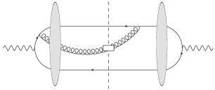
Figure 20: An example of diagram which contributes to the dipole $\times$ double dipole part of real contributions, in the gluon fragmentation case.

An example of dipole $\times$ double dipole contribution, in the gluon fragmentation case, is shown in Fig. 20. The complete dipole $\times$ double dipole contribution to the cross-section is

$$\frac{d\sigma_{JI}^{g\rightarrow h}}{dx_{h}d^{2}p_{h\perp}}\bigg{|}_{\text{dip. $\times$ d. dip.}}=\frac{\alpha_{em}}{2(2\pi)^{8}N_{c}\;x_{h}^{2}}\sum_{q}Q_{q}^{2}\int_{x_{h}}^{1}dx_{g}D_{g}^{h}\left(\frac{x_{h}}{x_{g}},\mu_{F}\right)\int\;d^{2}\vec{p}_{1}\;d^{2}\vec{p}_{2}\;d^{2}\vec{p}_{1^{\prime}}\;d^{2}\vec{p}_{2^{\prime}}$$

$$\times\int d^{2}\vec{p}_{3}\;d^{2}\vec{p}_{3^{\prime}}\int d^{2}\vec{p}_{\bar{q}}\int\frac{d^{2}\vec{p}_{q}}{(2\pi)^{2}}\int_{0}^{1-x_{g}}\frac{dx_{q}}{x_{q}}\frac{\delta\left(\vec{p}_{11^{\prime}}+\vec{p}_{22^{\prime}}+\vec{p}_{33^{\prime}}\right)}{(1-x_{q}-x_{g})}\delta\left(\frac{x_{g}}{x_{h}}\vec{p}_{h}+\vec{p}_{q1}+\vec{p}_{\bar{q}2}-\vec{p}_{3}\right)$$

$$\times\varepsilon_{I\alpha}\varepsilon_{J\beta}^{\ast}\frac{\alpha_{s}}{4(p_{\gamma}^{+})^{2}}\left[\Phi_{3}^{\alpha}(\vec{p}_{1},\vec{p}_{2})\Phi_{4}^{\beta\ast}(\vec{p}_{1^{\prime}},\vec{p}_{2^{\prime}},\vec{p}_{3^{\prime}})\mathbf{F}\left(\frac{\vec{p}_{12}}{2}\right)\widetilde{\mathbf{F}}^{\ast}\left(\frac{\vec{p}_{1^{\prime}2^{\prime}}}{2},\vec{p}_{3^{\prime}}\right)\delta(\vec{p}_{3})\right.$$

$$+\left.\Phi_{4}^{\alpha}(\vec{p}_{1},\vec{p}_{2},\vec{p}_{3})\Phi_{3}^{\beta\ast}(\vec{p}_{1^{\prime}},\vec{p}_{2^{\prime}})\widetilde{\mathbf{F}}\left(\frac{\vec{p}_{12}}{2},\vec{p}_{3}\right)\mathbf{F}^{\ast}\left(\frac{\vec{p}_{1^{\prime}2^{\prime}}}{2}\right)\delta(\vec{p}_{3^{\prime}})\right]\;.$$ (113)

6.2.4 Double dipole $\times$ double dipole contribution

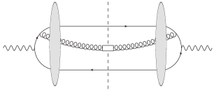
Figure 21: An example of diagram which contributes to the double dipole $\times$ double dipole part of real contributions, in the gluon fragmentation case.

The last contribution to be taken into account is the double dipole $\times$ double dipole one (see Fig. 21), which reads

$$\frac{d\sigma_{JI}^{g\rightarrow h}}{dx_{h}d^{2}p_{h\perp}}\bigg{|}_{\text{d. dip. $\times$ d. dip.}}=\frac{\alpha_{em}}{2(2\pi)^{8}(N_{c}^{2}-1)\;x_{h}^{2}}\sum_{q}Q_{q}^{2}\int_{x_{h}}^{1}dx_{g}D_{g}^{h}\left(\frac{x_{h}}{x_{g}},\mu_{F}\right)\int d^{2}\vec{p}_{1}d^{2}\vec{p}_{2}d^{2}\vec{p}_{1^{\prime}}d^{2}\vec{p}_{2^{\prime}}$$

$$\times\int\frac{d^{2}\vec{p}_{3}}{(2\pi)^{2}}\;\frac{d^{2}\vec{p}_{3^{\prime}}}{(2\pi)^{2}}\int d^{2}\vec{p}_{\bar{q}}\int\frac{d^{2}\vec{p}_{q}}{(2\pi)^{2}}\int_{0}^{1-x_{g}}dx_{q}\frac{\delta\left(\vec{p}_{11^{\prime}}+\vec{p}_{22^{\prime}}+\vec{p}_{33^{\prime}}\right)}{x_{q}(1-x_{q}-x_{g})}\delta\left(\frac{x_{g}}{x_{h}}\vec{p}_{h}+\vec{p}_{q1}+\vec{p}_{\bar{q}2}-\vec{p}_{3}\right)$$

$$\times\varepsilon_{I\alpha}\varepsilon_{J\beta}^{\ast}\frac{\alpha_{s}}{4(p_{\gamma}^{+})^{2}}\Phi_{4}^{\alpha}\left(\vec{p}_{1},\vec{p}_{2},\vec{p}_{3}\right)\Phi_{4}^{\beta\ast}(\vec{p}_{1^{\prime}},\vec{p}_{2^{\prime}},\vec{p}_{3^{\prime}})\widetilde{\mathbf{F}}\left(\frac{\vec{p}_{12}}{2},\vec{p}_{3}\right)\widetilde{\mathbf{F}}^{\ast}\left(\frac{\vec{p}_{1^{\prime}2^{\prime}}}{2},\vec{p}_{3^{\prime}}\right)\;.$$ (114)

7 Summary and Conclusion

In the present work, we have continued our study of diffractive processes in the saturation framework relying on the shockwave approach. In particular, we computed the cross section for the diffractive production of a hadron, at large $p_{T}$, in $\gamma^{(*)}$ nucleon/nucleus scattering, in rather general kinematics, which includes both lepto- and photoproduction. Our main result is the explicit proof of cancellation of any kind of divergences and the extraction of the finite remainder.

Diffractive productions are important channel to investigate the gluon tomography in the nucleon (see Marquet:2009ca ; Hatta:2022lzj ; Iancu:2021rup ) and the achievement of an appropriate level of precision calls for a full NLL description. This new class of processes provides an access to precision physics of gluon saturation dynamics, with very promising future phenomenological studies both at the LHC in UPC (in photoproduction) and at the future EIC (both in photoproduction and leptoproduction). It adds a new piece in the list of processes which are very promising to probe gluonic saturation in nucleons and nuclei at NLO, which includes inclusive DIS Beuf:2022ndu , inclusive photoproduction of dijets Altinoluk:2020qet ; Taels:2022tza , photon-dijet production in DIS Roy:2019hwr , dijets in DIS Caucal:2021ent ; Caucal:2022ulg ; Caucal:2023fsf , single hadron Bergabo:2022zhe and dihadrons production in DIS Bergabo:2022tcu ; Iancu:2022gpw , diffractive exclusive dijets Boussarie:2014lxa ; Boussarie:2016ogo ; Boussarie:2019ero and exclusive light meson production Boussarie:2016bkq ; Mantysaari:2022bsp , exclusive quarkonium production Mantysaari:2021ryb ; Mantysaari:2022kdm , inclusive DDIS Beuf:2022kyp , diffractive di-hadron production Fucilla:2022wcg , forward production of a Drell-Yan pair and a jet Taels:2023czt .

Appendix A LO impact factor squared

The impact factors in the LL, TL and TT cases are respectively given by

$$\sum_{\lambda_{q},\lambda_{\bar{q}}}\Phi_{0}^{+}(\vec{p}_{1},\vec{p}_{2})\Phi_{0}^{+*}(\vec{p}_{1^{\prime}},\vec{p}_{2^{\prime}})=\frac{32(p_{\gamma}^{+})^{4}x_{q}^{3}x_{\bar{q}}^{3}}{\left(\vec{p}_{q1}^{2}+x_{q}x_{\bar{q}}Q^{2}\right)\left(\vec{p}_{q1^{\prime}}^{2}+x_{q}x_{\bar{q}}Q^{2}\right)}\;,$$ (115)

$$\sum_{\lambda_{q},\lambda_{\bar{q}}}\Phi_{0}^{+}(\vec{p}_{1},\vec{p}_{2})\Phi_{0}^{i*}(\vec{p}_{1^{\prime}},\vec{p}_{2^{\prime}})=\frac{16(p_{\gamma}^{+})^{3}x_{q}^{2}x_{\bar{q}}^{2}p_{q1\perp}^{i}(1-2x_{q})}{\left(\vec{p}_{q1}^{2}+x_{q}x_{\bar{q}}Q^{2}\right)\left(\vec{p}_{q1^{\prime}}^{2}+x_{q}x_{\bar{q}}Q^{2}\right)}\;,$$ (116)

$$\sum_{\lambda_{q},\lambda_{\bar{q}}}\Phi_{0}^{i}(\vec{p}_{1},\vec{p}_{2})\Phi_{0}^{k*}(\vec{p}_{1^{\prime}},\vec{p}_{2^{\prime}})=\frac{8(p_{\gamma}^{+})^{2}x_{q}x_{\bar{q}}\left[(1-2x_{q})^{2}g_{\perp}^{ri}g_{\perp}^{lk}-g_{\perp}^{rk}g_{\perp}^{li}+g_{\perp}^{rl}g_{\perp}^{rl}g_{\perp}^{ik}\right]p_{q1\perp r}p_{q1^{\prime}\perp l}}{\left(\vec{p}_{q1}^{2}+x_{q}x_{\bar{q}}Q^{2}\right)\left(\vec{p}_{q1^{\prime}}^{2}+x_{q}x_{\bar{q}}Q^{2}\right)}\;.$$ (117)

The LT case is immediately obtained from TL by complex conjugation and $1,2\leftrightarrow 1^{\prime},2^{\prime}$ substitution.

Appendix B Finite parts of virtual corrections

B.1 Building blocks integrals

$$I_{1}^{k}(\vec{q}_{1},\,\vec{q}_{2},\,\Delta_{1},\,\Delta_{2}) \equiv \frac{1}{\pi}\int\frac{d^{d}\vec{l}\left(l_{\perp}^{k}\right)}{\left[(\vec{l}-\vec{q}_{1})^{2}+\Delta_{1}\right]\left[(\vec{l}-\vec{q}_{2})^{2}+\Delta_{2}\right]\vec{l}^{{}^{\,\,2}}},$$ (118)

$$I_{2}(\vec{q}_{1},\,\vec{q}_{2},\,\Delta_{1},\,\Delta_{2}) \equiv \frac{1}{\pi}\int\frac{d^{d}\vec{l}}{\left[(\vec{l}-\vec{q}_{1})^{2}+\Delta_{1}\right]\left[(\vec{l}-\vec{q}_{2})^{2}+\Delta_{2}\right]},$$ (119)

$$I_{3}^{k}(\vec{q}_{1},\,\vec{q}_{2},\,\Delta_{1},\,\Delta_{2}) \equiv \frac{1}{\pi}\int\frac{d^{d}\vec{l}\left(l_{\bot}^{k}\right)}{\left[(\vec{l}-\vec{q}_{1})^{2}+\Delta_{1}\right]\left[(\vec{l}-\vec{q}_{2})^{2}+\Delta_{2}\right]},$$ (120)

$$I^{jk}(\vec{q}_{1},\,\vec{q}_{2},\,\Delta_{1},\,\Delta_{2}) \equiv \frac{1}{\pi}\int\frac{d^{d}\vec{l}\left(l_{\perp}^{j}l_{\perp}^{k}\right)}{\left[(\vec{l}-\vec{q}_{1})^{2}+\Delta_{1}\right]\left[(\vec{l}-\vec{q}_{2})^{2}+\Delta_{2}\right]\vec{l}^{{}^{\,\,2}}}\,.$$ (121)

The arguments of these integrals will be different for each diagram so we will write them explicitly before giving the expression of each diagram, but we will omit them in the equations for the reader’s convenience.
Explicit results for the first 3 integrals in (118-121) are obtained by a straightforward Feynman parameter integration. We will express them using the following variables :

$$\rho_{1} \equiv \frac{\left(\vec{q}_{12}^{\,\,2}+\Delta_{12}\right)-\sqrt{\left(\vec{q}_{12}^{\,\,2}+\Delta_{12}\right)^{2}+4\vec{q}_{12}^{\,\,2}\Delta_{2}}}{2\vec{q}_{12}^{\,\,2}},$$ (122)

$$\rho_{2} \equiv \frac{\left(\vec{q}_{12}^{\,\,2}+\Delta_{12}\right)+\sqrt{\left(\vec{q}_{12}^{\,\,2}+\Delta_{12}\right)^{2}+4\vec{q}_{12}^{\,\,2}\Delta_{2}}}{2\vec{q}_{12}^{\,\,2}}\,,$$ (123)

where $\Delta_{ij}=\Delta_{i}-\Delta_{j}$ .
One gets :

$$I_{1}^{k} = \frac{q_{1\perp}^{k}}{2\left[\vec{q}_{12}^{\,\,2}\left(\vec{q}_{1}^{\,\,2}+\Delta_{1}\right)\left(\vec{q}_{2}^{\,\,2}+\Delta_{2}\right)-\left(\vec{q}_{1}^{\,\,2}-\vec{q}_{2}^{\,\,2}+\Delta_{12}\right)\left(\vec{q}_{1}^{\,\,2}\Delta_{2}-\vec{q}_{2}^{\,\,2}\Delta_{1}\right)\right]}$$

$$\times \left\{\frac{\left(\vec{q}_{2}^{\,\,2}+\Delta_{2}\right)\vec{q}_{12}^{\,\,2}+\vec{q}_{2}^{\,\,2}\left(\Delta_{1}+\Delta_{2}\right)+\Delta_{2}\left(\Delta_{21}-2\vec{q}_{1}^{\,\,2}\right)}{\left(\rho_{1}-\rho_{2}\right)\vec{q}_{12}^{\,\,2}}\ln\left[\left(\frac{-\rho_{1}}{1-\rho_{1}}\right)\left(\frac{1-\rho_{2}}{-\rho_{2}}\right)\right]\right.$$

$$\times \left.\left(\vec{q}_{2}^{\,\,2}+\Delta_{2}\right)\ln\left[\frac{\Delta_{2}\left(\vec{q}_{1}^{\,\,2}+\Delta_{1}\right)^{2}}{\Delta_{1}\left(\vec{q}_{2}^{\,\,2}+\Delta_{2}\right)^{2}}\right]+\left(1\leftrightarrow 2\right)\right\}\,,$$

$$I_{2} = \frac{1}{\vec{q}_{12}^{\,\,2}\left(\rho_{1}-\rho_{2}\right)}\ln\left[\left(\frac{-\rho_{1}}{1-\rho_{1}}\right)\left(\frac{1-\rho_{2}}{-\rho_{2}}\right)\right]\,,$$ (125)

and

$$I_{3}^{k} = \frac{\left(\vec{q}_{12}^{\,\,2}+\Delta_{12}\right)q_{1}^{k}+\left(\vec{q}_{21}^{\,\,2}+\Delta_{21}\right)q_{2}^{k}}{2\left(\rho_{1}-\rho_{2}\right)(\vec{q}_{12}^{\,\,2})^{2}}\ln\left[\left(\frac{-\rho_{1}}{1-\rho_{1}}\right)\left(\frac{1-\rho_{2}}{-\rho_{2}}\right)\right]$$ (126)

$$- \frac{q_{12}^{k}}{2\vec{q}_{12}^{\,\,2}}\ln\left(\frac{\Delta_{1}}{\Delta_{2}}\right)\,.$$

Please note that in some cases the real part of $\Delta_{1}$ or $\Delta_{2}$ will be negative so the previous results can acquire an imaginary part from the imaginary part $\pm\,i0$ of the arguments.
The last integral in (121) can be expressed in terms of the other ones by writing

$$I^{jk}=I_{11}\left(q_{1\perp}^{j}q_{1\perp}^{k}\right)+I_{12}\left(q_{1\perp}^{j}q_{2\perp}^{k}+q_{2\perp}^{j}q_{1\perp}^{k}\right)+I_{22}\left(q_{2\perp}^{j}q_{2\perp}^{k}\right)\,,$$ (127)

with

$$I_{11} =-\frac{1}{2}\frac{\left[\vec{q}_{2}^{\,\,2}q_{1\perp k}-\left(\vec{q}_{1}\cdot\vec{q}_{2}\right)q_{2\perp k}\right]}{\left[\vec{q}_{1}^{\,\,2}\vec{q}_{2}^{\,\,2}-\left(\vec{q}_{1}\cdot\vec{q}_{2}\right)^{2}\right]^{2}}$$ (128)

$$\times\left[\left(\frac{\vec{q}_{1}\cdot\vec{q}_{2}}{\vec{q}_{1}^{\,\,2}}\right)\ln\left(\frac{\vec{q}_{1}^{\,\,2}+\Delta_{1}}{\Delta_{1}}\right)q_{1\perp}^{k}+\left(\vec{q}_{2}\cdot\vec{q}_{21}\right)I_{3}^{k}+\left\{\vec{q}_{2}^{\,\,2}\left(\vec{q}_{1}\cdot\vec{q}_{12}\right)+\Delta_{1}\vec{q}_{2}^{\,\,2}-\Delta_{2}\left(\vec{q}_{1}\cdot\vec{q}_{2}\right)\right\}I_{1}^{k}\right]$$

$$I_{12} =\frac{-1}{4\left[\vec{q}_{1}^{\,\,2}\vec{q}_{2}^{\,\,2}-\left(\vec{q}_{1}\cdot\vec{q}_{2}\right)^{2}\right]}\ln\left(\frac{\vec{q}_{1}^{\,\,2}+\Delta_{1}}{\Delta_{1}}\right)$$

$$+\frac{\vec{q}_{2}^{\,\,2}\left(\vec{q}_{1}\cdot\vec{q}_{2}\right)}{2\left[\vec{q}_{1}^{\,\,2}\vec{q}_{2}^{\,\,2}-\left(\vec{q}_{1}\cdot\vec{q}_{2}\right)^{2}\right]^{2}}\left[\left(\vec{q}_{1}^{\,\,2}+\Delta_{1}\right)\left(q_{1\perp k}I_{1}^{k}\right)+\left(q_{1\perp k}I_{3}^{k}\right)\right]$$

$$-\frac{\left(\vec{q}_{1}^{\,\,2}\vec{q}_{2}^{\,\,2}\right)+\left(\vec{q}_{1}\cdot\vec{q}_{2}\right)^{2}}{4\left[\vec{q}_{1}^{\,\,2}\vec{q}_{2}^{\,\,2}-\left(\vec{q}_{1}\cdot\vec{q}_{2}\right)^{2}\right]^{2}}\left[\left(\vec{q}_{2}^{\,\,2}+\Delta_{2}\right)\left(q_{1\perp k}I_{1}^{k}\right)+\left(q_{1\perp k}I_{3}^{k}\right)\right]+(1\leftrightarrow 2),$$ (129)

$$I_{22} =I_{11}|_{1\leftrightarrow 2}\,.$$ (130)

In what follows, for the $\phi$ function, $x=x_{q}$, $\bar{x}=x_{\bar{q}}$.

B.2 $\phi_{4}$

The arguments in the integrals of B.1 are

$$\vec{q}_{1} = \vec{p}_{1}-\left(\frac{x-z}{x}\right)\vec{p}_{q},\quad\,\,\,\,\,\vec{q}_{2}=\left(\frac{x-z}{x}\right)\left(x\vec{p}_{\bar{q}}-\bar{x}\vec{p}_{q}\right)\,,$$

$$\Delta_{1} = \left(x-z\right)\left(\bar{x}+z\right)Q^{2},\quad\Delta_{2}=-\frac{x\left(\bar{x}+z\right)}{\bar{x}\left(x-z\right)}\vec{q}^{2}-i0\,.$$

Let us write the impact factors in terms of these variables.
They read:
(longitudinal NLO) $\times$ (longitudinal LO) contribution :

$$\left(\phi_{4}\right)_{LL}=-\frac{4(x-z)(\bar{x}+z)}{z}[-\bar{x}(x-z)(z+1)I_{2}+q_{2\bot k}(2x^{2}-(2x-z)(z+1))I_{1}^{k}]\,,$$ (131)

(longitudinal NLO) $\times$ (transverse LO) contribution :

$$\left(\phi_{4}\right)_{LT}^{j}=(1-2x)p_{q1^{\prime}}{}_{\bot}^{j}\left(\phi_{4}\right)_{LL}-4(x-z)(\bar{x}+z)(1-2x+z)[(\vec{q}\cdot\vec{p}_{q1^{\prime}})g_{\bot k}^{j}+q_{2\bot}^{j}p_{q1^{\prime}\bot k}]I_{1}^{k}\,,$$ (132)

(transverse NLO) $\times$ (longitudinal LO) contribution :

$$\left(\phi_{4}\right)_{TL}^{i} =2\{[(x-\bar{x}-z)q_{2\bot}^{i}q_{1\bot k}+(-8x\bar{x}-6xz+2z^{2}+3z+1)q_{1\perp}^{j}q_{2\bot k}]I_{1}^{k}$$

$$-2[4x^{2}-x(3z+5)+(z+1)^{2}]q_{2\bot k}I^{ik}+(x-\bar{x}-z)\left(\vec{q}_{2}\cdot\vec{q}_{1}\right)I^{i}$$

$$+I_{2}[(x-\bar{x}-z)q_{2\bot}^{i}+\bar{x}(2(x-z)^{2}-5x+3z+1)q_{1\perp}^{i}]$$

$$-\bar{x}[2(x-z)^{2}-5x+3z+1]I_{3}^{i}$$

$$+\frac{x\bar{x}(1-2x)}{z}[2q_{2\bot k}I^{ik}+I_{3}^{i}-q_{1\perp}^{i}(2q_{2\bot k}I_{1}^{k}+I_{2})]\}\,,$$ (133)

(transverse NLO) $\times$ (transverse LO) contribution :

$$\left(\phi_{4}\right)_{TT}^{ij} = \left[(x-\bar{x}-2z)(x-\bar{x}-z)(\vec{q}_{2}\cdot\vec{p}_{q1^{\prime}})q_{1\perp}^{i}+(z+1)(\left(\vec{q}_{1}\cdot\vec{q}_{2}\right)p_{q1^{\prime}\perp}^{i}-(\vec{q}_{1}\cdot\vec{p}_{q1^{\prime}})q_{2\bot}^{i})\right]I_{1}^{j}$$ (134)

$$+ 2\bar{x}[q_{2\bot k}-(x-z)q_{1\perp k}](p_{q1^{\prime}\bot}^{i}I^{jk}-g_{\bot}^{ij}p_{q1^{\prime}\bot l}I^{kl})$$

$$+ 2(x-z)[(2\bar{x}+z)(\vec{q}_{2}\cdot\vec{p}_{q1^{\prime}})-\bar{x}(\vec{q}_{1}\cdot\vec{p}_{q1^{\prime}})]I^{ij}$$

$$+ [(1-z)((\vec{q}_{1}\cdot\vec{p}_{q1^{\prime}})q_{2\bot}^{j}-(\vec{q}_{2}\cdot\vec{p}_{q1^{\prime}})q_{1\perp}^{j})-(1-2x)(\bar{x}-x+z)\left(\vec{q}_{1}\cdot\vec{q}_{2}\right)p_{q1^{\prime}\perp}^{j}]I_{1}^{i}$$

$$- 2\left[(x-z)(\bar{x}q_{1\perp}^{j}-(2\bar{x}+z)q_{2\bot}^{j})p_{q1^{\prime}\perp k}\right.$$

$$+ \left.(1-2x)\left(4x^{2}-(3z+5)x+(z+1)^{2}\right)q_{2\bot k}p_{q1^{\prime}}{}_{\bot}^{j}\right]I^{ik}$$

$$- \bar{x}\left(\bar{x}-x\right)\left(2(x-z)^{2}-5x+3z+1\right)p_{q1^{\prime}\perp}^{j}I_{3}^{i}$$

$$+ \bar{x}\left(\bar{x}+z\right)(p_{q1^{\prime}\perp}^{i}I_{3}^{j}-g_{\bot}^{ij}p_{q1^{\prime}\perp k}I_{3}^{k})$$

$$+ I_{2}\left[g_{\bot}^{ij}\left((1-z)(\vec{q}_{2}\cdot\vec{p}_{q1^{\prime}})-\bar{x}(1+x-z)(\vec{q}_{1}\cdot\vec{p}_{q1^{\prime}})\right)\right.$$

$$+ \left.((1-z)q_{2\bot}^{j}-\bar{x}(1+x-z)q_{1\perp}^{j})p_{q1^{\prime}}{}_{\bot}^{i}\right.$$

$$- \left.(\bar{x}-x)\left((\bar{x}-x+z)q_{2\bot}^{i}-\bar{x}\left(2(x-z)^{2}-5x+3z+1\right)q_{1\perp}^{i}\right)p_{q1^{\prime}}{}_{\bot}^{j}\right]$$

$$+ I_{1}^{k}\left[g_{\bot}^{ij}\left((x-\bar{x}+z)(\vec{q}_{1}\cdot\vec{p}_{q1^{\prime}})q_{2\bot k}+(1-z)(\vec{q}_{2}\cdot\vec{p}_{q1^{\prime}})q_{1\bot k}-(z+1)\left(\vec{q}_{1}\cdot\vec{q}_{2}\right)p_{q1^{\prime}}{}_{\bot k}\right)\right.$$

$$+ q_{1\perp}^{j}((x-\bar{x}+z)q_{2\bot k}p_{q1^{\prime}\perp}^{i}-(z+1)q_{2\bot}^{i}p_{q1^{\prime}}{}_{\bot k})$$

$$+ q_{2\bot}^{j}((x-\bar{x}-2z)(x-\bar{x}-z)q_{1\perp}^{i}p_{q1^{\prime}\perp k}+(1-z)q_{1\perp k}p_{q1^{\prime}}{}_{\bot}^{i})$$

$$- \left.(1-2x)((1-2x+z)q_{2\bot}^{i}q_{1\perp k}-(2z^{2}+3z-x(8\bar{x}+6z)+1)q_{1\perp}^{i}q_{2\bot k})p_{q1^{\prime}}{}_{\bot}^{j}\right]$$

$$+ \frac{x\bar{x}}{z}\left[(x-\bar{x})^{2}p_{q1^{\prime}\perp}^{j}(2q_{2\bot k}I^{ik}+I_{3}^{i}-q_{1\perp}^{i}(I_{2}+2q_{2\bot k}I_{1}^{k}))\right.$$

$$+ p_{q1^{\prime}\perp}^{i}(q_{1\perp}^{j}(I_{2}+2q_{2\bot k}I_{1}^{k})-2q_{2\bot k}I^{jk}-I_{3}^{j})$$

$$+ \left.g_{\bot}^{ij}((\vec{q}_{1}\cdot\vec{p}_{q1^{\prime}})(I_{2}+2q_{2\bot k}I_{1}^{k})+p_{q1^{\prime}\perp k}(2q_{2\bot l}I^{kl}+I_{3}^{k}))\right]\,.$$

B.3 $\phi_{5}$

Here the integrals from B.1 will have the following arguments :

$$\vec{q}_{1}=\left(\frac{x-z}{x}\right)\vec{p}_{3}-\frac{z}{x}\vec{p}_{1},\quad\vec{q}_{2}=\vec{p}_{q1}-\frac{z}{x}\vec{p}_{q}\,,$$ (135)

$$\Delta_{1}=\frac{z(x-z)}{x^{2}\bar{x}}(\vec{p}_{\bar{q}2}^{\,\,2}+x\bar{x}Q^{2}),\quad\Delta_{2}=(x-z)(\bar{x}+z)Q^{2}\,,$$ (136)

With such variables, it is easy to see that the argument in the square roots in (123) are full squares. In terms of the variables in (135), the impact factors read:
(longitudinal NLO) $\times$ (longitudinal LO) :

$$\left(\phi_{5}\right)_{LL}=\frac{4(x-z)(-2x(\bar{x}+z)+z^{2}+z)}{xz}\left[\bar{x}(x-z)I_{2}-\left(zq_{1\perp k}-x\left(\bar{x}+z\right)q_{2\bot k}\right)I_{1}^{k}\right]\,,$$ (137)

(longitudinal NLO) $\times$ (transverse LO) :

$$\left(\phi_{5}\right)_{LT}^{j} =(\bar{x}-x)p_{q1^{\prime}\bot}^{j}\left(\phi_{5}\right)_{LL}$$ (138)

$$+\frac{4(x-z)(x-\bar{x}-z)}{x}\left(zq_{1\perp}^{k}-x(\bar{x}+z)q_{2\perp}^{k}\right)p_{q1^{\prime}\perp l}\left(g_{\perp k}^{j}I_{1}^{l}+I_{1}^{j}\right)\,,$$

(transverse NLO) $\times$ (longitudinal LO) :

$$\left(\phi_{5}\right)_{TL}^{i} =2\left[(x-\bar{x}-z)\left(\vec{q}_{1}\cdot\vec{q}_{2}\right)-\bar{x}(x-z)^{2}Q^{2}+(\frac{z}{x}-x)\vec{q}_{1}^{\,\,2}\right]I_{1}^{i}$$

$$+\frac{2}{x}\left[xq_{2\bot k}(-8x\bar{x}-6xz+2z^{2}+3z+1)+2q_{1\bot k}(2xz-2x^{2}+x-z^{2})\right]q_{1\perp}^{i}I_{1}^{k}$$

$$+2q_{2\bot}^{i}q_{1\perp k}(x-\bar{x}-z)I_{1}^{k}+2\frac{\bar{x}}{x}(x(8x-3)-6xz+2z^{2}+z)I_{1}^{i}$$

$$+\frac{2}{x}\left[xq_{2\bot}^{i}(x-\bar{x}-z)+q_{1\perp}^{i}(8x^{3}-6x^{2}(z+2)+x(z+3)(2z+1)-2z^{2})\right]I_{2}$$

$$-\frac{4}{x}\left[(x-z)(\bar{x}+z)q_{1\perp k}+x(4x^{2}-x(3z+5)+(z+1)^{2})q_{2\perp k}\right]I^{ik}$$

$$-\frac{4}{z}x\bar{x}(x-\bar{x})\left[q_{2\perp k}I^{ik}+I_{3}^{i}-q_{1\perp}^{i}\left(q_{2\perp k}I_{1}^{k}+I_{2}\right)\right]\,,$$ (139)

(transverse NLO) $\times$ (transverse LO) :

$$\left(\phi_{5}\right)_{TT}^{ij}=-2(x-z)\left[\frac{z}{x}(\vec{q}_{1}\cdot\vec{p}_{q1^{\prime}})-(2\bar{x}+z)(\vec{q}_{2}\cdot\vec{p}_{q1^{\prime}})\right]I^{ij}$$

$$+\left[-\bar{x}(x-z)^{2}Q^{2}p_{q1^{\prime}\perp}^{i}+(\bar{x}-x+2z)(\bar{x}-x+z)(\vec{q}_{2}\cdot\vec{p}_{q1^{\prime}})q_{1\perp}^{i}\right.$$

$$-\left.(\vec{q}_{1}\cdot\vec{p}_{q1^{\prime}})((z+1)q_{2\bot}^{i}-2\frac{z}{x}(2x-z)q_{1\perp}^{i})\right.$$

$$+\left.((z+1)\left(\vec{q}_{1}\cdot\vec{q}_{2}\right)-\left(x+\frac{z}{x}\right)\vec{r}^{\,\,2})p_{q1^{\prime}\bot}^{i}\right]I_{1}^{j}$$

$$-2\frac{\bar{x}}{x}(xq_{2\perp k}+(x-z)q_{1\perp k})\left(g_{\bot}^{ij}p_{q1^{\prime}\perp l}I^{kl}-p_{q1^{\prime}}{}_{\bot}^{i}I^{jk}\right)$$

$$+\left[\bar{x}\left(x-\bar{x}\right)(x-z)^{2}Q^{2}p_{q1^{\prime}\perp}^{j}-(z-1)(\vec{q}_{1}\cdot\vec{p}_{q1^{\prime}})q_{2\bot}^{j}\right.$$

$$+\left.(z-1)(\vec{q}_{2}\cdot\vec{p}_{q1^{\prime}})q_{1\perp}^{j}+\frac{x-\bar{x}}{x}\left((x^{2}-z)\vec{q}_{1}^{\,\,2}+x(\bar{x}-x+z)(\vec{q}_{1}\cdot\vec{q}_{2})\right)p_{q1^{\prime}\perp}^{k}\right]I_{1}^{i}$$

$$+2\left[\frac{x-\bar{x}}{x}\left(x(4x^{2}-(3z+5)x+(z+1)^{2})q_{2\bot k}+(x-z)(\bar{x}+z)q_{1\perp k}\right)p_{q1^{\prime}\perp}^{j}\right.$$

$$-\left.\frac{x-z}{x}\left(x(2x-z-2)q_{2\bot}^{j}+zq_{1\perp}^{j}\right)p_{q1^{\prime}\perp k}\right]I^{ik}$$

$$+\frac{\bar{x}\left(\bar{x}-x\right)}{x}\left(2z^{2}-6xz+z+x(8x-3)\right)p_{q1^{\prime}\perp}^{j}I_{3}^{i}$$

$$+\left[(x-\bar{x})\left((\bar{x}-x+z)q_{2\bot}^{i}+\left(6(z+2)x-8x^{2}-(z+3)(2z+1)+2\frac{z^{2}}{x}\right)q_{1\perp}^{i}r_{\bot}^{i}\right)p_{q1^{\prime}\perp}^{j}\right.$$

$$+\left.(1-z)(g_{\bot}^{ij}(\vec{q}_{2}\cdot\vec{p}_{q1^{\prime}})+q_{2\bot}^{k}p_{q1^{\prime}\perp}^{i})+(2x+z-3)(g_{\bot}^{ik}(\vec{q}_{1}\cdot\vec{p}_{q1^{\prime}})+q_{1\perp}^{k}p_{q1^{\prime}\perp}^{i})\right]I_{2}$$

$$+\left(3\bar{x}+z-\frac{z}{x}\right)p_{q1^{\prime}\perp}^{i}I_{3}^{k}-\frac{\bar{x}}{x}(3x-z)g_{\bot}^{ij}p_{q1^{\prime}\perp k}I_{3}^{k}$$

$$+\left[(x-\bar{x})p_{q1^{\prime}\perp}^{j}\left\{(\bar{x}-x+z)q_{2\bot}^{i}q_{1\perp k}-(2z^{2}-6xz+3z-8x\bar{x}+1)q_{2\perp k}q_{1\perp}^{i}\right.\right.$$

$$-\left.2(\bar{x}-x+2z-\frac{z^{2}}{x})q_{1\perp k}q_{1\perp}^{i}\right\}+\bar{x}(x-z)^{2}Q^{2}g_{\bot}^{ij}p_{q1^{\prime}\perp k}$$

$$+(1-z)q_{1\perp k}(g_{\bot}^{ij}(\vec{q}_{2}\cdot\vec{p}_{q1^{\prime}})+q_{2\bot}^{j}p_{q1^{\prime}\perp}^{i})$$

$$+\left((x-\bar{x}+z)q_{2\bot k}-2q_{1\perp k}\right)(g_{\bot}^{ij}(\vec{q}_{1}\cdot\vec{p}_{q1^{\prime}})+q_{1\perp}^{j}p_{q1^{\prime}\perp}^{i})$$

$$+g_{\bot}^{ij}\left(\left(x+\frac{z}{x}\right)\vec{q}_{1}^{\,\,2}-(z+1)(\vec{q}_{1}\cdot\vec{q}_{2})\right)p_{q1^{\prime}\perp k}$$

$$+\left.\left((x-\bar{x}-2z)(x-\bar{x}-z)q_{1\perp}^{i}q_{2\perp}^{j}-(z+1)q_{2\perp}^{i}q_{1\perp}^{j}+2(2x-z)\frac{z}{x}q_{1\perp}^{i}q_{1\perp}^{j}\right)p_{q1^{\prime}\perp k}\right]I_{1}^{k}$$

$$+\frac{2x\bar{x}}{z}\left[(x-\bar{x})^{2}p_{q1^{\prime}\perp}^{j}(q_{2\bot k}I^{ik}+I_{3}^{i})-p_{q1^{\prime}\perp}^{i}(q_{2\bot k}I^{jk}+I_{3}^{k})+g_{\bot}^{ij}p_{q1^{\prime}\bot k}(q_{2\bot l}I^{kl}+I_{3}^{k})\right.$$

$$+\left.(I_{2}+q_{2\perp k}I_{1}^{k})\left(g_{\bot}^{ij}(\vec{q}_{1}\cdot\vec{p}_{q1^{\prime}})+q_{1\perp}^{j}p_{q1^{\prime}\perp}^{i}-(1-2x)^{2}q_{1\perp}^{i}p_{q1^{\prime}\perp}^{j}\right)\right].$$ (140)

B.4 $\phi_{6}$

We will use the variable

$$\vec{q}=\left(\frac{x-z}{x}\right)\vec{p}_{3}-\frac{z}{x}\vec{p}_{1}\,.$$ (141)

(longitudinal NLO) $\times$ (longitudinal NLO) :

$$(\phi_{6})_{LL}=-4x\bar{x}^{2}J_{0}\,,$$ (142)

(longitudinal NLO) $\times$ (transverse NLO) :

$$(\phi_{6})_{LT}^{j}=(1-2x)p_{q1^{\prime}\bot}^{j}(\phi_{6})_{LL}\,,$$ (143)

(transverse NLO) $\times$ (longitudinal NLO) :

$$(\phi_{6})_{TL}^{i}=2\bar{x}\left[(1-2x)p_{\bar{q}2\bot}^{i}J_{0}-J_{1\bot}^{i}\right]\,,$$ (144)

(transverse NLO) $\times$ (transverse NLO) :

$$(\phi_{6})_{TT}^{ij} =\bar{x}\left[(x-\bar{x})^{2}p_{\bar{q}2\bot}^{i}p_{q1^{\prime}\bot}^{j}-g_{\bot}^{ij}(\vec{p}_{\bar{q}2}\cdot\vec{p}_{q1^{\prime}})-p_{q1^{\prime}\bot}^{i}p_{\bar{q}2\bot}^{j}\right]J_{0}$$

$$+\bar{x}\left[(x-\bar{x})p_{q1^{\prime}\bot}^{j}g_{\bot k}^{i}-p_{q1^{\prime}\bot k}g_{\bot}^{ij}+p_{q1^{\prime}\bot}^{i}g_{\bot k}^{j}\right]J_{1\bot}^{k}\,.$$ (145)

We introduced

$$J_{1\bot}^{k} =\frac{(x-z)^{2}}{x^{2}}\frac{q_{\bot}^{k}}{\vec{q}^{\,\,2}}\ln\left(\frac{\vec{p}_{\bar{q}2}^{\,\,2}+x\bar{x}Q^{2}}{\vec{p}_{\bar{q}2}^{\,\,2}+x\bar{x}Q^{2}+\frac{x^{2}\bar{x}}{z(x-z)}\vec{q}^{\,\,2}}\right),$$ (146)

$$\mathrm{and}$$

$$J_{0} =\frac{z}{x(\vec{p}_{\bar{q}2}^{\,\,2}+x\bar{x}Q^{2})}-\frac{2x(x-z)+z^{2}}{xz(\vec{p}_{\bar{q}2}^{\,\,2}+x\bar{x}Q^{2})}\ln\left(\frac{x^{2}\bar{x}\mu^{2}}{z(x-z)(\vec{p}_{\bar{q}2}^{\,\,2}+x\bar{x}Q^{2})+x^{2}\bar{x}\vec{q}^{\,\,2}}\right).$$ (147)

Appendix C Finite part of the squared impact factors for real corrections

C.1 LL transition

The double dipole $\times$ double dipole contribution is

$$\Phi {}_{4}^{+}(p_{1\bot},p_{2\bot},p_{3\bot})\Phi_{4}^{+*}(p_{1\bot}^{\prime},p_{2\bot}^{\prime},p_{3\bot}^{\prime})=\frac{8p_{\gamma}^{+}{}^{4}}{z^{2}\left(\frac{\vec{p}_{\bar{q}2^{\prime}}^{\,\,2}}{x_{\bar{q}}\left(1-x_{\bar{q}}\right)}+Q^{2}\right)\left(Q^{2}+\frac{\vec{p}_{q1^{\prime}}^{\,\,2}}{x_{q}}+\frac{\vec{p}_{\bar{q}2^{\prime}}^{\,\,2}}{x_{\bar{q}}}+\frac{\vec{p}_{g3^{\prime}}^{\,\,2}}{z}\right)}$$

$$\times \left[\frac{x_{\bar{q}}\left(dz^{2}+4x_{q}\left(x_{q}+z\right)\right)\left(x_{q}\vec{p}_{g3}-z\vec{p}_{q1})(x_{q}\vec{p}_{g3^{\prime}}-z\vec{p}_{q1^{\prime}}\right)}{x_{q}\left(x_{q}+z\right)^{2}{}\left(\frac{(\vec{p}_{g3}+\vec{p}_{q1}){}^{2}}{x_{\bar{q}}\left(x_{q}+z\right)}+Q^{2}\right)\left(\frac{(\vec{p}_{g3}+\vec{p}_{q1}){}^{2}}{x_{\bar{q}}}+\frac{\vec{p}_{g3}^{\,\,2}}{z}+\frac{\vec{p}_{q1}^{\,\,2}}{x_{q}}+Q^{2}\right)}\right.$$

$$- \left.\frac{(4x_{q}x_{\bar{q}}+2z-dz^{2})(x_{\bar{q}}\vec{p}_{g3}-z\vec{p}_{\bar{q}2})(x_{q}\vec{p}_{g3^{\prime}}-z\vec{p}_{q1^{\prime}})}{\left(x_{\bar{q}}+z\right)\left(x_{q}+z\right)\left(\frac{(\vec{p}_{\bar{q}2}+\vec{p}_{g3}){}^{2}}{x_{q}\left(x_{\bar{q}}+z\right)}+Q^{2}\right)\left(\frac{(\vec{p}_{\bar{q}2}+\vec{p}_{g3}){}^{2}}{x_{q}}+\frac{\vec{p}_{g3}^{\,\,2}}{z}+\frac{\vec{p}_{\bar{q}2}^{\,\,2}}{x_{\bar{q}}}+Q^{2}\right)}\right]+(q\leftrightarrow\bar{q}).$$ (148)

The interference term in the dipole $\times$ dipole contribution reads

$$\left(\tilde{\Phi}_{3}^{+}(\vec{p}_{1},\vec{p}_{2})\Phi_{4}^{+*}(\vec{p}_{1^{\prime}},\vec{p}_{2^{\prime}},\vec{0})+\Phi_{4}^{+}(\vec{p}_{1},\vec{p}_{2},\vec{0})\tilde{\Phi}_{3}^{+*}(\vec{p}_{1^{\prime}},\vec{p}_{2^{\prime}})\right)$$

$$=\left[\frac{8p_{\gamma}^{+}{}^{4}}{z\left(x_{q}+z\right)\left(\frac{\vec{p}{}_{\bar{q}2^{\prime}}^{\,\,2}}{x_{\bar{q}}\left(x_{q}+z\right)}+Q^{2}\right)\left(\frac{\vec{p}{}_{q1^{\prime}}^{\,\,2}}{x_{q}}+\frac{\vec{p}{}_{\bar{q}2^{\prime}}^{\,\,2}}{x_{\bar{q}}}+\frac{\vec{p}_{g}{}^{2}}{z}+Q^{2}\right)}\right.$$

$$\times\left\{\frac{\left(4x_{q}x_{\bar{q}}+z(2-dz)\right)(\vec{p}_{g}-\frac{z}{x_{\bar{q}}}\vec{p}_{\bar{q}})(x_{q}\vec{p}_{g}-z\vec{p}_{q1^{\prime}})}{(\vec{p}_{g}-\frac{z\vec{p}_{\bar{q}}}{x_{\bar{q}}}){}^{2}\left(\frac{\vec{p}{}_{q1^{\prime}}^{\,\,2}}{x_{q}\left(x_{\bar{q}}+z\right)}+Q^{2}\right)}\right.$$

$$-\left.\left.\frac{x_{\bar{q}}\left(dz^{2}+4x_{q}\left(x_{q}+z\right)\right)({}\vec{p}_{g}-\frac{z}{x_{q}}\vec{p}_{q})(\vec{p}_{g}-\frac{z}{x_{q}}\vec{p}_{q1^{\prime}})}{(\vec{p}_{g}-\frac{z\vec{p}_{q}}{x_{q}}){}^{2}\left(\frac{\vec{p}{}_{\bar{q}2}^{\,\,2}}{x_{\bar{q}}\left(x_{q}+z\right)}+Q^{2}\right)}\right\}+(q\leftrightarrow\bar{q})\right]$$

$$+(1\leftrightarrow 1^{\prime},2\leftrightarrow 2^{\prime}).$$ (149)

The double dipole $\times$ dipole contribution has the form

$$\Phi_{4}^{+}(\vec{p}_{1},\vec{p}_{2},\vec{p}_{3})\,\Phi_{3}^{+*}(\vec{p}_{1^{\prime}},\vec{p}_{2^{\prime}})=\Phi_{4}^{+}(\vec{p}_{1},\vec{p}_{2},\vec{p}_{3})\Phi_{4}^{+*}(\vec{p}_{1^{\prime}},\vec{p}_{2^{\prime}},\vec{0})+\Phi_{4}^{+}(\vec{p}_{1},\vec{p}_{2},\vec{p}_{3})\tilde{\Phi}_{3}^{+*}(\vec{p}_{1^{\prime}},\vec{p}_{2^{\prime}}),$$ (150)

where

$$\Phi_{4}^{+}(\vec{p}_{1},\vec{p}_{2},\vec{p}_{3}) \tilde{\Phi}_{3}^{+*}(\vec{p}_{1^{\prime}},\vec{p}_{2^{\prime}})=\frac{8p_{\gamma}^{+}{}^{4}}{z\left(x_{q}+z\right)\left(\frac{\vec{p}{}_{\bar{q}2}^{\,\,2}}{x_{\bar{q}}\left(x_{q}+z\right)}+Q^{2}\right)\left(\frac{\vec{p}{}_{q1}^{\,\,2}}{x_{q}}+\frac{\vec{p}{}_{\bar{q}2}^{\,\,2}}{x_{\bar{q}}}+\frac{\vec{p}_{g3}^{\,\,2}}{z}+Q^{2}\right)}$$

$$\times\left\{\frac{\left(4x_{q}x_{\bar{q}}+z(2-dz)\right)(\vec{p}_{g}-\frac{z}{x_{\bar{q}}}\vec{p}_{\bar{q}})(x_{q}\vec{p}_{g3}-z\vec{p}_{q1})}{(\vec{p}_{g}-\frac{z\vec{p}_{\bar{q}}}{x_{\bar{q}}}){}^{2}\left(\frac{\vec{p}{}_{q1^{\prime}}^{\,\,2}}{x_{q}\left(x_{\bar{q}}+z\right)}+Q^{2}\right)}\right.$$

$$-\left.\frac{x_{\bar{q}}\left(dz^{2}+4x_{q}\left(x_{q}+z\right)\right)(\vec{p}_{g}-\frac{z}{x_{q}}\vec{p}_{q})(\vec{p}_{g3}-\frac{z}{x_{q}}\vec{p}_{q1})}{(\vec{p}_{g}-\frac{z\vec{p}_{q}}{x_{q}}){}^{2}\left(\frac{\vec{p}{}_{\bar{q}2^{\prime}}^{\,\,2}}{x_{\bar{q}}\left(x_{q}+z\right)}+Q^{2}\right)}\right\}+(q\leftrightarrow\bar{q}).$$ (151)

For the dipole $\times$ double dipole contribution, one just has to complex conjugate (151) and also invert the name of the momenta i.e. $1^{\prime},2^{\prime}\leftrightarrow 1,2$.

C.2 LT/TL transition

The double dipole $\times$ double dipole contribution is

$$\Phi_{4}^{i}(p_{1\bot},p_{2\bot},p_{3\bot})\Phi_{4}^{+*}(p_{1\bot}^{\prime},p_{2\bot}^{\prime},p_{3\bot}^{\prime})$$

$$=\frac{-4p_{\gamma}^{+}{}^{3}}{\left(Q^{2}+\frac{\vec{p}{}_{g3}^{\,\,2}}{z}+\frac{\vec{p}{}_{q1}^{\,\,2}}{x_{q}}+\frac{\vec{p}{}_{{\bar{q}}2}^{\,\,2}}{x_{\bar{q}}}\right)\left(Q^{2}+\frac{\vec{p}{}_{g3^{\prime}}^{\,\,2}}{z}+\frac{\vec{p}{}_{q1^{\prime}}^{\,\,2}}{x_{q}}+\frac{\vec{p}{}_{{\bar{q}}2^{\prime}}^{\,\,2}}{x_{\bar{q}}}\right)}$$

$$\times\left(\frac{z\left((\vec{P}\cdot\vec{p}_{q1})G_{\bot}^{i}-(\vec{G}\cdot\vec{p}_{q1})P_{\bot}^{i}\right)\left(dz+4x_{q}-4\right)-(\vec{G}\cdot\vec{P})p_{q1}^{i}{}_{\bot}\left(2x_{q}-1\right)\left(4\left(x_{q}-1\right)x_{\bar{q}}-dz^{2}\right)}{z^{2}x_{\bar{q}}\left(z+x_{\bar{q}}\right){}^{3}\left(Q^{2}+\frac{\vec{p}{}_{q1}^{\,\,2}}{x_{q}\left(z+x_{\bar{q}}\right)}\right)\left(Q^{2}+\frac{\vec{p}{}_{q1^{\prime}}^{\,\,2}}{x_{q}\left(z+x_{\bar{q}}\right)}\right)}\right.$$

$$+\frac{z\left((\vec{P}\cdot\vec{p}_{q1})H_{\bot}^{i}-(\vec{H}\cdot\vec{p}_{q1})P_{\bot}^{i}\right)\left(dz+4x_{q}-2\right)-(\vec{H}\cdot\vec{P})p_{q1}^{i}{}_{\bot}\left(2x_{q}-1\right)\left(z(2-dz)+4x_{q}x_{\bar{q}}\right)}{z^{2}x_{q}\left(z+x_{q}\right)\left(z+x_{\bar{q}}\right){}^{2}\left(Q^{2}+\frac{\vec{p}{}_{\bar{q}2^{\prime}}^{\,\,2}}{\left(z+x_{q}\right)x_{\bar{q}}}\right)\left(Q^{2}+\frac{\vec{p}{}_{q1}^{\,\,2}}{x_{q}\left(z+x_{\bar{q}}\right)}\right)}$$

$$+\left.\frac{H_{\bot}^{i}\left(z(zd+d-2)+x_{q}\left(2-4x_{\bar{q}}\right)\right)x_{\bar{q}}}{z\left(z+x_{q}\right){}^{2}\left(z+x_{\bar{q}}\right)\left(Q^{2}+\frac{\vec{p}{}_{\bar{q}2^{\prime}}^{\,\,2}}{\left(z+x_{q}\right)x_{\bar{q}}}\right)}\right)+(q\leftrightarrow\bar{q}).$$ (152)

Here,

$$G_{\bot}^{i}=x_{\bar{q}}p_{g3^{\prime}\bot}^{i}-zp_{\bar{q}2^{\prime}\bot}^{i},\quad H_{\bot}^{i}=x_{q}p_{g3^{\prime}\bot}^{i}-zp_{q1^{\prime}\bot}^{i},\quad P_{\bot}^{i}=x_{\bar{q}}p_{g3\bot}^{i}-zp_{\bar{q}2\bot}^{i}.$$ (153)

The interference term in the dipole $\times$ dipole contribution reads

$$\left(\Phi_{4}^{i}(\vec{p}_{1},\vec{p}_{2},\vec{0})\tilde{\Phi}_{3}^{+*}(\vec{p}_{1^{\prime}},\vec{p}_{2^{\prime}})+\tilde{\Phi}_{3}^{i}(\vec{p}_{1},\vec{p}_{2})\Phi_{4}^{+*}(\vec{p}_{1^{\prime}},\vec{p}_{2^{\prime}},\vec{0})\right)$$

$$=4p_{\gamma}^{+}{}^{3}\left(\frac{\Delta_{q}{}_{\bot}^{i}x_{q}x_{\bar{q}}\left(dz^{2}+dz-2z+2x_{q}-4x_{q}x_{\bar{q}}\right)}{\vec{\Delta}{}_{q}^{2}\left(z+x_{q}\right){}^{2}\left(z+x_{\bar{q}}\right)\left(Q^{2}+\frac{\vec{p}_{g}^{\,\,2}}{z}+\frac{\vec{p}{}_{q1}^{\,\,2}}{x_{q}}+\frac{\vec{p}{}_{\bar{q}2}^{\,\,2}}{x_{\bar{q}}}\right)\left(Q^{2}+\frac{\vec{p}{}_{\bar{q}2^{\prime}}^{\,\,2}}{\left(z+x_{q}\right)x_{\bar{q}}}\right)}\right.$$

$$-\frac{(\vec{J}\cdot\vec{\Delta}_{q})p_{\bar{q}2}^{i}{}_{\bot}\left(dz^{2}+4x_{q}\left(z+x_{q}\right)\right)\left(1-2x_{\bar{q}}\right)+z\left((\vec{J}\cdot\vec{p}_{\bar{q}2})\Delta_{q}^{i}{}_{\bot}-(\vec{p}_{\bar{q}2}\cdot\vec{\Delta}_{q})J_{\bot}^{i}\right)\left(dz+4x_{\bar{q}}-4\right)}{z\left(z+x_{q}\right){}^{3}\vec{\Delta}{}_{q}^{2}\left(Q^{2}+\frac{\vec{p}_{g}^{\,\,2}}{z}+\frac{\vec{p}{}_{q1^{\prime}}^{\,\,2}}{x_{q}}+\frac{\vec{p}{}_{\bar{q}2^{\prime}}^{\,\,2}}{x_{\bar{q}}}\right)\left(Q^{2}+\frac{\vec{p}{}_{\bar{q}2}^{\,\,2}}{\left(z+x_{q}\right)x_{\bar{q}}}\right)\left(Q^{2}+\frac{\vec{p}{}_{\bar{q}2^{\prime}}^{\,\,2}}{\left(z+x_{q}\right)x_{\bar{q}}}\right)}$$

$$-\frac{x_{q}\left(z\left((\vec{K}\cdot\vec{p}_{\bar{q}2})\Delta_{q}^{i}{}_{\bot}-(\vec{p}_{\bar{q}2}\cdot\vec{\Delta}_{q})K_{\bot}^{i}\right)\left(dz+4x_{\bar{q}}-2\right)+(\vec{K}\cdot\vec{\Delta}_{q})p_{\bar{q}2}^{i}{}_{\bot}\left(1-2x_{\bar{q}}\right)\left(z(dz-2)-4x_{q}x_{\bar{q}}\right)\right)}{z\left(z+x_{q}\right){}^{2}x_{\bar{q}}\left(z+x_{\bar{q}}\right)\vec{\Delta}{}_{q}^{2}\left(Q^{2}+\frac{\vec{p}_{g}^{\,\,2}}{z}+\frac{\vec{p}{}_{q1^{\prime}}^{\,\,2}}{x_{q}}+\frac{\vec{p}{}_{\bar{q}2^{\prime}}^{\,\,2}}{x_{\bar{q}}}\right)\left(Q^{2}+\frac{\vec{p}{}_{\bar{q}2}^{\,\,2}}{\left(z+x_{q}\right)x_{\bar{q}}}\right)\left(Q^{2}+\frac{\vec{p}{}_{q1^{\prime}}^{\,\,2}}{x_{q}\left(z+x_{\bar{q}}\right)}\right)}$$

$$-\frac{z\left((\vec{p}_{q1}\cdot\vec{\Delta}_{q})X_{\bot}^{i}-(\vec{X}\cdot\vec{p}_{q1})\Delta_{q}^{i}{}_{\bot}\right)\left(dz+4x_{q}-2\right)+(\vec{X}\cdot\vec{\Delta}_{q})p_{q1}^{i}{}_{\bot}\left(1-2x_{q}\right)\left(z(dz-2)-4x_{q}x_{\bar{q}}\right)}{z\vec{\Delta}{}_{q}^{2}\left(z+x_{q}\right)\left(z+x_{\bar{q}}\right){}^{2}\left(Q^{2}+\frac{\vec{p}_{g}^{\,\,2}}{z}+\frac{\vec{p}{}_{q1}^{\,\,2}}{x_{q}}+\frac{\vec{p}{}_{\bar{q}2}^{\,\,2}}{x_{\bar{q}}}\right)\left(Q^{2}+\frac{\vec{p}{}_{\bar{q}2^{\prime}}^{\,\,2}}{\left(z+x_{q}\right)x_{\bar{q}}}\right)\left(Q^{2}+\frac{\vec{p}{}_{q1}^{\,\,2}}{x_{q}\left(z+x_{\bar{q}}\right)}\right)}$$

$$+\left.\frac{z\left((\vec{X}\cdot\vec{p}_{q1})\Delta_{\bar{q}}^{i}{}_{\bot}-(\vec{p}_{q1}\cdot\vec{\Delta}_{\bar{q}})X_{\bot}^{i}\right)\left(dz+4x_{q}-4\right)-(\vec{X}\cdot\vec{\Delta}_{\bar{q}})p_{q1}^{i}{}_{\bot}\left(2x_{q}-1\right)\left(4\left(x_{q}-1\right)x_{\bar{q}}-dz^{2}\right)}{z\left(z+x_{\bar{q}}\right){}^{3}\vec{\Delta}{}_{\bar{q}}^{2}\left(Q^{2}+\frac{\vec{p}_{g}^{\,\,2}}{z}+\frac{\vec{p}{}_{q1}^{\,\,2}}{x_{q}}+\frac{\vec{p}{}_{\bar{q}2}^{\,\,2}}{x_{\bar{q}}}\right)\left(Q^{2}+\frac{\vec{p}{}_{q1}^{\,\,2}}{x_{q}\left(z+x_{\bar{q}}\right)}\right)\left(Q^{2}+\frac{\vec{p}{}_{q1^{\prime}}^{\,\,2}}{x_{q}\left(z+x_{\bar{q}}\right)}\right)}\right)$$

$$+(q\leftrightarrow\bar{q})\;,$$ (154)

where

$$\vec{\Delta}_{q}=\frac{x_{q}\vec{p}_{g}-x_{g}\vec{p}_{q}}{x_{q}+x_{g}}\vec{\Delta}_{\bar{q}}=\frac{x_{\bar{q}}\vec{p}_{g}-x_{g}\vec{p}_{\bar{q}}}{x_{q}+x_{g}}$$ (155)

$$X_{\bot}^{i}=x_{\bar{q}}p_{g\bot}^{i}-zp_{\bar{q}2\bot}^{i}= P_{\bot}^{i}|_{p_{3}=0},\quad J_{\bot}^{i}=x_{q}p_{g\bot}^{i}-zp_{q1^{\prime}\bot}^{i}=H_{\bot}^{i}|_{p_{3}^{\prime}=0},$$

$$K_{\bot}^{i} =x_{\bar{q}}p_{g\bot}^{i}-zp_{\bar{q}2^{\prime}\bot}^{i}=G_{\bot}^{i}|_{p_{3}^{\prime}=0}.$$ (156)

The TL transition is obtained from above by complex conjugation and inverting the naming of the different momenta in (154) and (152).
The double dipole $\times$ dipole have, respectively, the form

$$\Phi_{4}^{i}(\vec{p}_{1},\vec{p}_{2},\vec{p}_{3})\Phi_{3}^{+*}(\vec{p}_{1^{\prime}},\vec{p}_{2^{\prime}})=\Phi_{4}^{i}(\vec{p}_{1},\vec{p}_{2},\vec{p}_{3})\Phi_{4}^{+*}(\vec{p}_{1^{\prime}},\vec{p}_{2^{\prime}},0)+\Phi_{4}^{i}(\vec{p}_{1},\vec{p}_{2},\vec{p}_{3})\tilde{\Phi}_{3}^{+*}(\vec{p}_{1^{\prime}},\vec{p}_{2^{\prime}})\;,$$ (157)

$$\Phi_{4}^{+}(\vec{p}_{1},\vec{p}_{2},\vec{p}_{3})\Phi_{3}^{i*}(\vec{p}_{1^{\prime}},\vec{p}_{2^{\prime}})=\Phi_{4}^{+}(\vec{p}_{1},\vec{p}_{2},\vec{p}_{3})\Phi_{4}^{i*}(\vec{p}_{1^{\prime}},\vec{p}_{2^{\prime}},\vec{0})+\Phi_{4}^{+}(\vec{p}_{1},\vec{p}_{2},\vec{p}_{3})\tilde{\Phi}_{3}^{i*}(\vec{p}_{1^{\prime}},\vec{p}_{2^{\prime}})\;,$$ (158)

where

$$\Phi_{4}^{i}(\vec{p}_{1},\vec{p}_{2},\vec{p}_{3})\tilde{\Phi}_{3}^{+*}(\vec{p}_{1^{\prime}},\vec{p}_{2^{\prime}})=\frac{4p_{\gamma}^{+}{}^{3}}{\left(x_{q}+z\right)\vec{\Delta}_{q}^{2}\left(\frac{\vec{p}{}_{\bar{q}2^{\prime}}^{\,\,2}}{x_{\bar{q}}\left(x_{q}+z\right)}+Q^{2}\right)\left(\frac{\vec{p}{}_{q1}^{\,\,2}}{x_{q}}+\frac{\vec{p}{}_{\bar{q}2}^{\,\,2}}{x_{\bar{q}}}+\frac{\vec{p}_{g3}^{\;2}}{z}+Q^{2}\right)}$$

$$\times\left\{\frac{x_{q}x_{\bar{q}}\Delta_{q}^{i}\left(dz(z+1)-2\left(1-2x_{q}\right)\left(x_{q}+z\right)\right)}{\left(x_{q}+z\right){}\left(x_{\bar{q}}+z\right)}+\frac{\left(dz+4x_{q}-2\right)\left(\Delta_{q}^{i}\vec{P}\cdot\vec{p}_{q1}-P^{i}\vec{p}_{q1}\cdot\vec{\Delta}_{q}\right)}{\left(x_{\bar{q}}+z\right){}^{2}\left(\frac{\vec{p}_{q1}^{\;2}}{x_{q}\left(x_{\bar{q}}+z\right)}+Q^{2}\right)}\right.$$

$$+\frac{\left(2x_{q}-1\right)p_{q1}^{i}\vec{P}\cdot\vec{\Delta}_{q}\left(z(dz-2)-4x_{q}x_{\bar{q}}\right)}{z\left(x_{\bar{q}}+z\right){}^{2}\left(\frac{\vec{p}_{q1}^{\;2}}{x_{q}\left(x_{\bar{q}}+z\right)}+Q^{2}\right)}-\frac{\left((d-4)z-4x_{q}\right)\left(W^{i}\vec{p}_{\bar{q}2}\cdot\vec{\Delta}_{q}-\Delta_{q}^{i}\vec{W}\cdot\vec{p}_{\bar{q}2}\right)}{\left(x_{q}+z\right){}^{2}\left(\frac{\vec{p}_{\bar{q}2}^{\;2}}{x_{\bar{q}}\left(x_{q}+z\right)}+Q^{2}\right)}$$

$$+\left.\frac{\left(2x_{\bar{q}}-1\right)\left(dz^{2}+4x_{q}\left(x_{q}+z\right)\right)p_{\bar{q}2}^{i}\vec{W}\cdot\vec{\Delta}_{q}}{z\left(x_{q}+z\right){}^{2}\left(\frac{\vec{p}_{\bar{q}2}^{\;2}}{x_{\bar{q}}\left(x_{q}+z\right)}+Q^{2}\right)}\right\}+(q\leftrightarrow\bar{q})\;,$$ (159)

and

$$\Phi_{4}^{+}(\vec{p}_{1},\vec{p}_{2},\vec{p}_{3}) \tilde{\Phi}_{3}^{i*}(\vec{p}_{1^{\prime}},\vec{p}_{2^{\prime}})=\frac{4p_{\gamma}^{+}{}^{3}}{z\vec{\Delta}{}_{q}^{2}\left(x_{q}+z\right){}^{2}\left(Q^{2}+\frac{\vec{p}_{g3}^{\,\,2}}{z}+\frac{\vec{p}{}_{q1}^{\,\,2}}{x_{q}}+\frac{\vec{p}{}_{\bar{q}2}^{\,\,2}}{x_{\bar{q}}}\right)\left(Q^{2}+\frac{\vec{p}{}_{\bar{q}2^{\prime}}^{\,\,2}}{\left(z+x_{q}\right)x_{\bar{q}}}\right)}$$

$$\times\left[\frac{x_{q}z\left((d-4)z-4x_{q}+2\right)\left(P^{i}\left(\vec{p}_{\bar{q}2^{\prime}}\cdot\vec{\Delta}_{q}\right)-\Delta_{q}^{i}\left(\vec{P}\cdot\vec{p}_{\bar{q}2^{\prime}}\right)\right)}{x_{\bar{q}}\left(x_{\bar{q}}+z\right)\left(\frac{\vec{p}_{q1}^{\;2}}{x_{q}\left(x_{\bar{q}}+z\right)}+Q^{2}\right)}\right.$$

$$-\frac{x_{q}\left(x_{q}-x_{\bar{q}}+z\right)p_{\bar{q}2^{\prime}}^{i}\left(\vec{P}\cdot\vec{\Delta}_{q}\right)\left(z(dz-2)-4x_{q}x_{\bar{q}}\right)}{x_{\bar{q}}\left(x_{\bar{q}}+z\right)\left(\frac{\vec{p}_{q1}^{\;2}}{x_{q}\left(x_{\bar{q}}+z\right)}+Q^{2}\right)}$$

$$-\frac{\left(x_{q}-x_{\bar{q}}+z\right)\left(dz^{2}+4x_{q}\left(x_{q}+z\right)\right)p_{\bar{q}2^{\prime}}^{i}\left(\vec{W}\cdot\vec{\Delta}_{q}\right)}{\left(x_{q}+z\right){}\left(\frac{\vec{p}_{\bar{q}2}^{\;2}}{x_{\bar{q}}\left(x_{q}+z\right)}+Q^{2}\right)}$$

$$-\left.\frac{z\left((d-4)z-4x_{q}\right)\left(\Delta_{q}^{i}\left(\vec{W}\cdot\vec{p}_{\bar{q}2^{\prime}}\right)-W^{i}\left(\vec{p}_{\bar{q}2^{\prime}}\cdot\vec{\Delta}_{q}\right)\right)}{\left(x_{q}+z\right){}\left(\frac{\vec{p}_{\bar{q}2}^{\,\,2}}{x_{\bar{q}}\left(x_{q}+z\right)}+Q^{2}\right)}\right]+(q\leftrightarrow\bar{q}).$$ (160)

Here, we introduced

$$W_{\bot}^{i}=x_{q}p_{g3\bot}^{i}-zp_{q1\bot}^{i}.$$ (161)

C.3 TT transition

The double dipole $\times$ double dipole contribution is

$$\Phi_{4}^{i}(p_{1\bot},p_{2\bot},p_{3\bot})\Phi_{4}^{k}(p_{1\bot}^{\prime},p_{2\bot}^{\prime},p_{3\bot}^{\prime})^{\ast}=\left(\frac{p_{\gamma}^{+}{}^{2}}{\left(Q^{2}+\frac{\vec{p}_{g3}^{\;2}}{z}+\frac{\vec{p}_{q1}^{\;2}}{x_{q}}+\frac{\vec{p}_{\bar{q}2}^{\,\,2}}{x_{\bar{q}}}\right)\left(Q^{2}+\frac{\vec{p}_{g3^{\prime}}^{\;2}}{z}+\frac{\vec{p}_{q1^{\prime}}^{\;2}}{x_{q}}+\frac{\vec{p}_{\bar{q}2^{\prime}}^{\,\,2}}{x_{\bar{q}}}\right)}\right.$$

$$\times\left[-\frac{g_{\bot}^{ik}x_{q}x_{\bar{q}}\left(zd+d-2+2x_{\bar{q}}\right)}{\left(z+x_{q}\right)^{2}\left(z+x_{\bar{q}}\right)}-\frac{2P_{\bot}^{k}p_{q1\bot}^{i}\left(1-2x_{q}\right)}{z\left(z+x_{\bar{q}}\right)^{2}\left(Q^{2}+\frac{\vec{p}_{q1}^{\;2}}{x_{q}\left(z+x_{\bar{q}}\right)}\right)}\left(\frac{(d-2)z-2x_{\bar{q}}}{z+x_{\bar{q}}}+\frac{dz+2x_{\bar{q}}}{z+x_{q}}\right)\right.$$

$$-\frac{2\left(g_{\bot}^{ik}(\vec{P}\cdot\vec{p}_{q1})+P_{\bot}^{i}p_{q1\bot}{}^{k}\right)}{z\left(z+x_{\bar{q}}\right)^{2}\left(Q^{2}+\frac{\vec{p}_{q1}^{\;2}}{x_{q}\left(z+x_{\bar{q}}\right)}\right)}\left(\frac{(d-4)z-2x_{\bar{q}}}{z+x_{q}}+\frac{(d-2)z-2x_{\bar{q}}}{z+x_{\bar{q}}}\right)$$

$$-\frac{1}{z^{2}x_{q}\left(z+x_{q}\right)^{2}x_{\bar{q}}\left(z+x_{\bar{q}}\right)^{2}\left(Q^{2}+\frac{\vec{p}_{\bar{q}2^{\prime}}^{\,\,2}}{\left(z+x_{q}\right)x_{\bar{q}}}\right)\left(Q^{2}+\frac{\vec{p}_{q1}^{\;2}}{x_{q}\left(z+x_{\bar{q}}\right)}\right)}\left\{(\vec{H}\cdot\vec{P})\left[p_{q1\bot}^{i}{}p_{\bar{q}2^{\prime}\bot}^{k}{}\left(1-2x_{q}\right)\right.\right.$$

$$\times\left.\left(1-2x_{\bar{q}}\right)\left(z(2-dz)+4x_{q}x_{\bar{q}}\right)+(g_{\bot}^{ik}(\vec{p}_{q1}\cdot\vec{p}_{\bar{q}2^{\prime}})+p_{q1\bot}^{k}p_{\bar{q}2^{\prime}\bot}^{i})\left(z(2-(d-4)z)+4x_{q}x_{\bar{q}}\right)\right]$$

$$+((d-4)z-2)\left[z(\vec{H}\cdot\vec{p}_{\bar{q}2^{\prime}})(g_{\bot}^{ik}(\vec{P}\cdot\vec{p}_{q1})+P_{\bot}^{i}p_{q1\bot}^{k})+zH_{\bot}^{k}\left((\vec{P}\cdot\vec{p}_{q1})p_{\bar{q}2^{\prime}\bot}^{i}-(\vec{p}_{q1}\cdot\vec{p}_{\bar{q}2^{\prime}})P_{\bot}^{i}\right)\right]$$

$$+((d-4)z+2)\left[zH^{i}\left((\vec{P}\cdot\vec{p}_{\bar{q}2^{\prime}})p_{q1\bot}^{k}-(\vec{p}_{q1}\cdot\vec{p}_{\bar{q}2^{\prime}})P_{\bot}^{k}\right)+z(\vec{H}\cdot\vec{p}_{q1})(g_{\bot}^{ik}(\vec{P}\cdot\vec{p}_{\bar{q}2^{\prime}})+P_{\bot}^{k}p_{\bar{q}2^{\prime}\bot}^{i})\right]$$

$$+\left.2z\left((\vec{H}\cdot\vec{p}_{\bar{q}2^{\prime}})P_{\bot}^{k}-(\vec{P}\cdot\vec{p}_{\bar{q}2^{\prime}})H_{\bot}^{k}\right)p_{q1\bot}{}^{i}\left(1-2x_{q}\right)\left(dz+4x_{\bar{q}}-2\right)\right\}$$

$$-\frac{1}{z^{2}x_{q}x_{\bar{q}}\left(z+x_{\bar{q}}\right){}^{4}\left(Q^{2}+\frac{\vec{p}_{q1}^{\;2}}{x_{q}\left(z+x_{\bar{q}}\right)}\right)\left(Q^{2}+\frac{\vec{p}_{q1^{\prime}}^{\;2}}{x_{q}\left(z+x_{\bar{q}}\right)}\right)}\left\{z\left((d-4)z-4x_{\bar{q}}\right)\frac{{}}{{}}\right.$$

$$\times\left[g_{\bot}^{ik}\left((\vec{G}\cdot\vec{p}_{q1^{\prime}})(\vec{P}\cdot\vec{p}_{q1})-(\vec{G}\cdot\vec{p}_{q1})(\vec{P}\cdot\vec{p}_{q1^{\prime}})\right)+(\vec{p}_{q1}\cdot\vec{p}_{q1^{\prime}})\left(G_{\bot}^{i}P_{\bot}^{k}-G_{\bot}^{k}P_{\bot}^{i}\right)\right.$$

$$+\left.2(\vec{G}\cdot\vec{p}_{q1^{\prime}})\left(P_{\bot}^{i}p_{q1\bot}^{k}+P_{\bot}^{k}p_{q1\bot}^{i}\left(1-2x_{q}\right)\right)-2(\vec{G}\cdot\vec{p}_{q1})\left(P_{\bot}^{k}p_{q1^{\prime}\bot}^{i}+P_{\bot}^{i}p_{q1^{\prime}\bot}^{k}\left(1-2x_{q}\right)\right)\right]$$

$$+\left.\left.(\vec{G}\cdot\vec{P})\left[p_{q1\bot}^{k}p_{q1^{\prime}\bot}^{i}-p_{q1\bot}^{i}p_{q1^{\prime}\bot}^{k}\left(1-2x_{q}\right)^{2}+g_{\bot}^{ik}\left(\vec{p}_{q1}\cdot\vec{p}_{q1^{\prime}}\right)\right]\left(dz^{2}+4x_{\bar{q}}\left(z+x_{\bar{q}}\right)\right)\right\}\right]$$

$$+\left.\frac{{}}{{}}(1\leftrightarrow 1^{\prime},2\leftrightarrow 2^{\prime},3\leftrightarrow 3^{\prime},i\leftrightarrow k)\right)+(q\leftrightarrow\bar{q}).$$ (162)

The interference term in the dipole $\times$ dipole contribution reads

$$\left(\tilde{\Phi}_{3}^{i}(\vec{p}_{1},\vec{p}_{2})\Phi_{4}^{k*}(\vec{p}_{1^{\prime}},\vec{p}_{2^{\prime}},\vec{0})+\Phi_{4}^{i}(\vec{p}_{1},\vec{p}_{2},\vec{0})\tilde{\Phi}_{3}^{k*}(\vec{p}_{1^{\prime}},\vec{p}_{2^{\prime}})\right)$$

$$=\left(\frac{2p_{\gamma}^{+}{}^{2}}{\vec{\Delta}{}_{q}^{2}\left(Q^{2}+\frac{\vec{p}_{g}^{\,\,2}}{z}+\frac{\vec{p}{}_{q1}^{\,\,2}}{x_{q}}+\frac{\vec{p}{}_{\bar{q}2}^{\,\,2}}{x_{\bar{q}}}\right)\left(Q^{2}+\frac{\vec{p}{}_{\bar{q}2^{\prime}}^{\,\,2}}{\left(z+x_{q}\right)x_{\bar{q}}}\right)}\right.$$

$$\times\left[\frac{\left((d-2)z-2x_{q}\right)x_{q}}{\left(z+x_{q}\right){}^{3}}\left(g_{\bot}^{ik}(\vec{p}_{\bar{q}2^{\prime}}\cdot\vec{\Delta}_{q})+p_{\bar{q}2^{\prime}}{}_{\bot}^{i}\Delta_{q\bot}^{k}+p_{\bar{q}2^{\prime}\bot}^{k}\Delta_{q\bot}^{i}\left(1-2x_{\bar{q}}\right)\right)\right.$$

$$+\frac{x_{q}\left(\left((d-4)z-2x_{q}\right)\left(g_{\bot}^{ik}(\vec{p}_{\bar{q}2^{\prime}}\cdot\vec{\Delta}_{q})+p_{\bar{q}2^{\prime}\bot}^{i}{}\Delta_{q\bot}^{k}{}\right)+p_{\bar{q}2^{\prime}\bot}^{k}\Delta_{q\bot}^{i}\left(dz+2x_{q}\right)\left(1-2x_{\bar{q}}\right)\right)}{\left(z+x_{q}\right){}^{2}\left(z+x_{\bar{q}}\right)}$$

$$-\frac{1}{z\left(z+x_{q}\right){}^{2}x_{\bar{q}}\left(z+x_{\bar{q}}\right){}^{2}\left(Q^{2}+\frac{\vec{p}_{q1}^{\;2}}{x_{q}\left(z+x_{\bar{q}}\right)}\right)}\left\{z((d-4)z+2)\frac{{}}{{}}\right.$$

$$\times\left[p_{q1}{}_{\bot}^{i}\left((\vec{p}_{\bar{q}2^{\prime}}\cdot\vec{\Delta}_{q})X_{\bot}^{k}-(\vec{X}\cdot\vec{p}_{\bar{q}2^{\prime}})\Delta_{q\bot}^{k}\right)\left(2x_{q}-1\right)-(\vec{X}\cdot\vec{p}_{\bar{q}2^{\prime}})\left(g_{\bot}^{ik}(\vec{p}_{q1}\cdot\vec{\Delta}_{q})+p_{q1\bot}^{k}\Delta_{q\bot}^{i}\right)\right.$$

$$\left.-X_{\bot}^{k}\left((\vec{p}_{q1}\cdot\vec{\Delta}_{q})p_{\bar{q}2^{\prime}\bot}^{i}-(\vec{p}_{q1}\cdot\vec{p}_{\bar{q}2^{\prime}})\Delta_{q}{}_{\bot}^{i}\right)\right]+4x_{q}z\left(1-2x_{q}\right)p_{q1\bot}^{i}\left((\vec{p}_{\bar{q}2^{\prime}}\cdot\vec{\Delta}_{q})X_{\bot}^{k}-(\vec{X}\cdot\vec{p}_{\bar{q}2^{\prime}})\Delta_{q\bot}^{k}\right)$$

$$+z\left(1-2x_{\bar{q}}\right)\left(dz+4x_{q}-2\right)p_{\bar{q}2^{\prime}\bot}^{k}\left((\vec{p}_{q1}\cdot\vec{\Delta}_{q})X_{\bot}^{i}-(\vec{X}\cdot\vec{p}_{q1})\Delta_{q\bot}^{i}\right)-z((d-4)z-2)$$

$$\times\left[\left(g_{\bot}^{ik}(\vec{X}\cdot\vec{p}_{q1})+X_{\bot}^{i}p_{q1\bot}^{k}\right)(\vec{p}_{\bar{q}2^{\prime}}\cdot\vec{\Delta}_{q})+\left((\vec{X}\vec{p}_{q1})p_{\bar{q}2^{\prime}}{}_{\bot}^{i}-(\vec{p}_{q1}\vec{p}_{\bar{q}2^{\prime}})X_{\bot}^{i}\right)\Delta_{q\bot}^{k}\right]$$

$$+(\vec{X}\cdot\vec{\Delta}_{q})p_{q1\bot}^{i}p_{\bar{q}2^{\prime}\bot}^{k}\left(1-2x_{q}\right)\left(1-2x_{\bar{q}}\right)\left(z(dz-2)-4x_{q}x_{\bar{q}}\right)$$

$$-\left.(\vec{X}\cdot\vec{\Delta}_{q})\left(g_{\bot}^{ik}(\vec{p}_{q1}\cdot\vec{p}_{\bar{q}2^{\prime}})+p_{q1\bot}^{k}p_{\bar{q}2^{\prime}\bot}^{i}\right)\left(z(2-(d-4)z)+4x_{q}x_{\bar{q}}\right)\right\}$$

$$-\frac{1}{z\left(z+x_{q}\right){}^{4}\left(Q^{2}+\frac{\vec{p}{}_{\bar{q}2}^{\,\,2}}{\left(z+x_{q}\right)x_{\bar{q}}}\right)x_{\bar{q}}}\left\{z\left(dz+4x_{\bar{q}}-4\right)\left[\left(1-2x_{\bar{q}}\right)\frac{{}}{{}}\right.\right.$$

$$\times\left(p_{\bar{q}2^{\prime}\bot}^{k}\left((\vec{p}_{\bar{q}2}\cdot\vec{\Delta}_{q})V_{\bot}^{i}-(\vec{V}\cdot\vec{p}_{\bar{q}2})\Delta_{q\bot}^{i}\right)+p_{\bar{q}2\bot}^{i}\left((\vec{V}\vec{p}_{\bar{q}2^{\prime}})\Delta_{q\bot}^{k}-(\vec{p}_{\bar{q}2^{\prime}}\cdot\vec{\Delta}_{q})V_{\bot}^{k}\right)\right)$$

$$+V_{\bot}^{k}\left((\vec{p}_{\bar{q}2}\cdot\vec{\Delta}_{q})p_{\bar{q}2^{\prime}\bot}^{i}-(\vec{p}_{\bar{q}2}\cdot\vec{p}_{\bar{q}2^{\prime}})\Delta_{q\bot}^{i}\right)+\left((\vec{p}_{\bar{q}2}\cdot\vec{p}_{\bar{q}2^{\prime}})V_{\bot}^{i}-(\vec{V}\cdot\vec{p}_{\bar{q}2})p_{\bar{q}2^{\prime}\bot}^{i}\right)\Delta_{q\bot}^{k}$$

$$+\left.g_{\bot}^{ik}\left((\vec{V}\cdot\vec{p}_{\bar{q}2^{\prime}})(\vec{p}_{\bar{q}2}\cdot\vec{\Delta}_{q})-(\vec{V}\cdot\vec{p}_{\bar{q}2})(\vec{p}_{\bar{q}2^{\prime}}\cdot\vec{\Delta}_{q})\right)+p_{\bar{q}2\bot}^{k}\left((\vec{V}\cdot\vec{p}_{\bar{q}2^{\prime}})\Delta_{q\bot}^{i}-(\vec{p}_{\bar{q}2^{\prime}}\cdot\vec{\Delta}_{q})V_{\bot}^{i}\right)\right]$$

$$+\left.\left.(\vec{V}\cdot\vec{\Delta}_{q})\left(p_{\bar{q}2\bot}^{i}p_{\bar{q}2^{\prime}\bot}^{k}\left(1-2x_{\bar{q}}\right)^{2}-g_{\bot}^{ik}(\vec{p}_{\bar{q}2}\cdot\vec{p}_{\bar{q}2^{\prime}})-p_{\bar{q}2\bot}^{k}p_{\bar{q}2^{\prime}\bot}^{i}\right)\left(dz^{2}-4x_{q}\left(x_{\bar{q}}-1\right)\right)\right\}\frac{{}}{{}}\right]$$

$$+\left.\frac{{}}{{}}(1\leftrightarrow 1^{\prime},2\leftrightarrow 2^{\prime},i\leftrightarrow k)\right)+(q\leftrightarrow\bar{q}).$$ (163)

Here,

$$V_{\bot}^{i}=x_{q}p_{g\bot}^{i}-zp_{q1\bot}^{i}.$$ (164)

The double dipole $\times$ dipole contribution has the form

$$\Phi_{4}^{i}(\vec{p}_{1},\vec{p}_{2},\vec{p}_{3})\,\Phi_{3}^{k*}(\vec{p}_{1^{\prime}},\vec{p}_{2^{\prime}})=\Phi_{4}^{i}(\vec{p}_{1},\vec{p}_{2},\vec{p}_{3})\Phi_{4}^{k*}(\vec{p}_{1^{\prime}},\vec{p}_{2^{\prime}},\vec{0})+\Phi_{4}^{i}(\vec{p}_{1},\vec{p}_{2},\vec{p}_{3})\tilde{\Phi}_{3}^{k*}(\vec{p}_{1^{\prime}},\vec{p}_{2^{\prime}}),$$ (165)

where

$$\Phi_{4}^{i}(\vec{p}_{1},\vec{p}_{2},\vec{p}_{3})\tilde{\Phi}_{3}^{k*}(\vec{p}_{1^{\prime}},\vec{p}_{2^{\prime}})$$

$$=\frac{2p_{\gamma}^{+}{}^{2}}{\vec{\Delta}{}_{q}^{2}\left(Q^{2}+\frac{\vec{p}_{g3}^{\,\,2}}{z}+\frac{\vec{p}{}_{q1}^{\,\,2}}{x_{q}}+\frac{\vec{p}{}_{\bar{q}2}^{\,\,2}}{x_{\bar{q}}}\right)\left(Q^{2}+\frac{\vec{p}{}_{\bar{q}2^{\prime}}^{\,\,2}}{\left(z+x_{q}\right)x_{\bar{q}}}\right)}$$

$$\times\left[\frac{\left((d-2)z-2x_{q}\right)x_{q}}{\left(z+x_{q}\right){}^{3}}\left(g_{\bot}^{ik}(\vec{p}_{\bar{q}2^{\prime}}\vec{\Delta}_{q})+p_{\bar{q}2^{\prime}}{}_{\bot}^{i}\Delta_{q\bot}{}^{k}+p_{\bar{q}2^{\prime}\bot}{}^{k}\Delta_{q\bot}{}^{i}\left(1-2x_{\bar{q}}\right)\right)\right.$$

$$+\frac{x_{q}\left(\left((d-4)z-2x_{q}\right)\left(g_{\bot}^{ik}(\vec{p}_{\bar{q}2^{\prime}}\vec{\Delta}_{q})+p_{\bar{q}2^{\prime}\bot}^{i}{}\Delta_{q\bot}^{k}{}\right)+p_{\bar{q}2^{\prime}\bot}^{k}{}\Delta_{q\bot}^{i}{}\left(dz+2x_{q}\right)\left(1-2x_{\bar{q}}\right)\right)}{\left(z+x_{q}\right){}^{2}\left(z+x_{\bar{q}}\right)}$$

$$-\frac{1}{z\left(z+x_{q}\right){}^{2}x_{\bar{q}}\left(z+x_{\bar{q}}\right){}^{2}\left(Q^{2}+\frac{\vec{p}_{q1}^{\;2}}{x_{q}\left(z+x_{\bar{q}}\right)}\right)}\left\{z((d-4)z+2)\frac{{}}{{}}\right.$$

$$\times\left[p_{q1}{}_{\bot}^{i}\left((\vec{p}_{\bar{q}2^{\prime}}\vec{\Delta}_{q})P_{\bot}^{k}-(\vec{P}\vec{p}_{\bar{q}2^{\prime}})\Delta_{q}{}_{\bot}^{k}\right)\left(2x_{q}-1\right)-(\vec{P}\vec{p}_{\bar{q}2^{\prime}})\left(g_{\bot}^{ik}(\vec{p}_{q1}\vec{\Delta}_{q})+p_{q1}{}_{\bot}^{k}\Delta_{q}{}_{\bot}^{i}\right)\right.$$

$$-\!\left.P_{\bot}^{k}\!\left(\!(\vec{p}_{q1}\vec{\Delta}_{q})p_{\bar{q}2^{\prime}}{}_{\bot}^{i}\!-\!(\vec{p}_{q1}\vec{p}_{\bar{q}2^{\prime}})\Delta_{q}{}_{\bot}^{i}\!\right)\!\right]+4x_{q}z\left(1-2x_{q}\right)p_{q1}{}_{\bot}^{i}\!\left(\!(\vec{p}_{\bar{q}2^{\prime}}\vec{\Delta}_{q})P_{\bot}^{k}-(\vec{P}\vec{p}_{\bar{q}2^{\prime}})\Delta_{q}{}_{\bot}^{k}\!\right)$$

$$+z\left(1-2x_{\bar{q}}\right)\left(dz+4x_{q}-2\right)p_{\bar{q}2^{\prime}}{}_{\bot}^{k}\left((\vec{p}_{q1}\vec{\Delta}_{q})P_{\bot}^{i}-(\vec{P}\vec{p}_{q1})\Delta_{q}{}_{\bot}^{i}\right)-z((d-4)z-2)$$

$$\times\left[\left(g_{\bot}^{ik}(\vec{P}\vec{p}_{q1})+P_{\bot}^{i}p_{q1}{}_{\bot}^{k}\right)(\vec{p}_{\bar{q}2^{\prime}}\vec{\Delta}_{q})+\left((\vec{P}\vec{p}_{q1})p_{\bar{q}2^{\prime}}{}_{\bot}^{i}-(\vec{p}_{q1}\vec{p}_{\bar{q}2^{\prime}})P_{\bot}^{i}\right)\Delta_{q}{}_{\bot}^{k}\right]$$

$$+(\vec{P}\vec{\Delta}_{q})p_{q1}{}_{\bot}^{i}p_{\bar{q}2^{\prime}}{}_{\bot}^{k}\left(1-2x_{q}\right)\left(1-2x_{\bar{q}}\right)\left(z(dz-2)-4x_{q}x_{\bar{q}}\right)$$

$$-\left.(\vec{P}\vec{\Delta}_{q})\left(g_{\bot}^{ik}(\vec{p}_{q1}\vec{p}_{\bar{q}2^{\prime}})+p_{q1}{}_{\bot}^{k}p_{\bar{q}2^{\prime}}{}_{\bot}^{i}\right)\left(z(2-(d-4)z)+4x_{q}x_{\bar{q}}\right)\right\}\;.$$ (166)

As above, the dipole $\times$ double dipole contribution is obtained by complex conjugation and changing the momenta.

References

- (1) V. S. Fadin, E. A. Kuraev, and L. N. Lipatov, On the Pomeranchuk Singularity in Asymptotically Free Theories, Phys. Lett. B60 (1975) 50–52.
- (2) E. A. Kuraev, L. N. Lipatov, and V. S. Fadin, Multi - Reggeon Processes in the Yang-Mills Theory, Sov. Phys. JETP 44 (1976) 443–450.
- (3) E. A. Kuraev, L. N. Lipatov, and V. S. Fadin, The Pomeranchuk Singularity in Nonabelian Gauge Theories, Sov. Phys. JETP 45 (1977) 199–204.
- (4) I. I. Balitsky and L. N. Lipatov, The Pomeranchuk Singularity in Quantum Chromodynamics, Sov. J. Nucl. Phys. 28 (1978) 822–829.
- (5) V. S. Fadin and L. N. Lipatov, BFKL pomeron in the next-to-leading approximation, Phys. Lett. B429 (1998) 127–134, [hep-ph/9802290].
- (6) M. Ciafaloni and G. Camici, Energy scale(s) and next-to-leading BFKL equation, Phys. Lett. B430 (1998) 349–354, [hep-ph/9803389].
- (7) V. Fadin and R. Fiore, Non-forward BFKL pomeron at next-to-leading order, Phys. Lett. B610 (2005) 61–66, [hep-ph/0412386].
- (8) V. S. Fadin and R. Fiore, Non-forward NLO BFKL kernel, Phys. Rev. D72 (2005) 014018, [hep-ph/0502045].
- (9) F. G. Celiberto, Hunting BFKL in semi-hard reactions at the LHC, Eur. Phys. J. C 81, no.8, 691 (2021), [arXiv:2008.07378].
- (10) L. D. McLerran and R. Venugopalan, Computing quark and gluon distribution functions for very large nuclei, Phys. Rev. D 49 (1994), 2233-2241 [hep-ph/9509289].
- (11) I. Balitsky, Operator expansion for high-energy scattering, Nucl. Phys. B463 (1996) 99–160, [hep-ph/9509348].
- (12) I. Balitsky, Factorization for high-energy scattering, Phys. Rev. Lett. 81 (1998) 2024–2027, [hep-ph/9807434].
- (13) I. Balitsky, Factorization and high-energy effective action, Phys. Rev. D60 (1999) 014020, [hep-ph/9812311].
- (14) I. Balitsky, Effective field theory for the small-x evolution, Phys. Lett. B518 (2001) 235–242, [hep-ph/0105334].
- (15) J. Jalilian-Marian, A. Kovner, A. Leonidov, and H. Weigert, The BFKL equation from the Wilson renormalization group, Nucl. Phys. B504 (1997) 415–431, [hep-ph/9701284].
- (16) J. Jalilian-Marian, A. Kovner, A. Leonidov, and H. Weigert, The Wilson renormalization group for low x physics: Towards the high density regime, Phys. Rev. D59 (1999) 014014, [hep-ph/9706377].
- (17) J. Jalilian-Marian, A. Kovner, and H. Weigert, The Wilson renormalization group for low x physics: Gluon evolution at finite parton density, Phys. Rev. D59 (1999) 014015, [hep-ph/9709432].
- (18) J. Jalilian-Marian, A. Kovner, A. Leonidov, and H. Weigert, Unitarization of gluon distribution in the doubly logarithmic regime at high density, Phys. Rev. D59 (1999) 034007, [hep-ph/9807462].
- (19) A. Kovner, J. G. Milhano, and H. Weigert, Relating different approaches to nonlinear QCD evolution at finite gluon density, Phys. Rev. D62 (2000) 114005, [hep-ph/0004014].
- (20) H. Weigert, Unitarity at small Bjorken x, Nucl. Phys. A703 (2002) 823–860, [hep-ph/0004044].
- (21) E. Iancu, A. Leonidov, and L. D. McLerran, Nonlinear gluon evolution in the color glass condensate. I, Nucl. Phys. A692 (2001) 583–645, [hep-ph/0011241].
- (22) E. Iancu, A. Leonidov, and L. D. McLerran, The renormalization group equation for the color glass condensate, Phys. Lett. B510 (2001) 133–144, [hep-ph/0102009].
- (23) E. Ferreiro, E. Iancu, A. Leonidov, and L. McLerran, Nonlinear gluon evolution in the color glass condensate. II, Nucl. Phys. A703 (2002) 489–538, [hep-ph/0109115].
- (24) Y. V. Kovchegov, Small- structure function of a nucleus including multiple pomeron exchanges, Phys. Rev. D60 (1999) 034008, [hep-ph/9901281].
- (25) Y. V. Kovchegov, Unitarization of the BFKL pomeron on a nucleus, Phys. Rev. D61 (2000) 074018, [hep-ph/9905214].
- (26) G. A. Chirilli and Y. V. Kovchegov, Solution of the NLO BFKL Equation and a Strategy for Solving the All-Order BFKL Equation, JHEP 06 (2013) 055, [arXiv:1305.1924].
- (27) A. V. Grabovsky, On the solution to the NLO forward BFKL equation, JHEP 09 (2013) 098, [arXiv:1307.3152].
- (28) R. Boussarie, A. Grabovsky, L. Szymanowski, and S. Wallon, Impact factor for high-energy two and three jets diffractive production, JHEP 1409 (2014) 026, [arXiv:1405.7676].
- (29) R. Boussarie, A. V. Grabovsky, L. Szymanowski, and S. Wallon, On the one loop impact factor and the exclusive diffractive cross sections for the production of two or three jets, JHEP 11 (2016) 149, [arXiv:1606.00419].
- (30) R. Boussarie, A. V. Grabovsky, L. Szymanowski, and S. Wallon, Towards a complete next-to-logarithmic description of forward exclusive diffractive dijet electroproduction at HERA: real corrections, Phys. Rev. D100 (2019), no. 7 074020, [arXiv:1905.07371].
- (31) R. Boussarie, A. V. Grabovsky, D. Yu. Ivanov, L. Szymanowski, and S. Wallon, Next-to-Leading Order Computation of Exclusive Diffractive Light Vector Meson Production in a Saturation Framework, Phys. Rev. Lett. 119 (2017), no. 7 072002, [arXiv:1612.08026].
- (32) M. Fucilla, A. V. Grabovsky, E. Li, L. Szymanowski and S. Wallon, NLO computation of diffractive di-hadron production in a saturation framework, JHEP 03 (2023), 159, [arXiv:2211.05774].
- (33) G. Altarelli, R. K. Ellis, G. Martinelli, and S.-Y. Pi, Processes Involving Fragmentation Functions Beyond the Leading Order in QCD, Nucl. Phys. B 160 (1979) 301–329.
- (34) V. N. Gribov and L. N. Lipatov, Deep inelastic e p scattering in perturbation theory, Sov. J. Nucl. Phys. 15 (1972) 438–450.
- (35) L. N. Lipatov, The parton model and perturbation theory, Sov. J. Nucl. Phys. 20 (1975) 94–102.
- (36) G. Altarelli and G. Parisi, Asymptotic freedom in parton language, Nucl. Phys. B126 (1977) 298.
- (37) Y. L. Dokshitzer, Calculation of the Structure Functions for Deep Inelastic Scattering and Annihilation by Perturbation Theory in Quantum Chromodynamics, Sov. Phys. JETP 46 (1977) 641–653.
- (38) D. Yu. Ivanov and A. Papa, Inclusive production of a pair of hadrons separated by a large interval of rapidity in proton collisions, JHEP 07 (2012) 045, [arXiv:1205.6068].
- (39) G. A. Chirilli, B.-W. Xiao, and F. Yuan, Inclusive Hadron Productions in pA Collisions, Phys. Rev. D86 (2012) 054005, [arXiv:1203.6139].
- (40) Y. Hatta, B. W. Xiao and F. Yuan, Semi-inclusive diffractive deep inelastic scattering at small x, Phys. Rev. D 106 (2022) no.9, 094015 [arXiv:2205.08060].
- (41) C. Marquet, B. W. Xiao and F. Yuan, Semi-inclusive Deep Inelastic Scattering at small x, Phys. Lett. B 682 (2009), 207-211 [arXiv:0906.1454].
- (42) E. Iancu, A. H. Mueller and D. N. Triantafyllopoulos, Probing Parton Saturation and the Gluon Dipole via Diffractive Jet Production at the Electron-Ion Collider, Phys. Rev. Lett. 128 (2022) no.20, 202001 [arXiv:2112.06353].
- (43) G. Beuf, T. Lappi and R. Paatelainen, Massive quarks in NLO dipole factorization for DIS: Transverse photon, Phys. Rev. D 106 (2022) no.3, 034013 [arXiv:2204.02486].
- (44) T. Altinoluk, R. Boussarie, C. Marquet and P. Taels, Photoproduction of three jets in the CGC: gluon TMDs and dilute limit, JHEP 07 (2020), 143 [arXiv:2001.00765]
- (45) P. Taels, T. Altinoluk, G. Beuf and C. Marquet, Dijet photoproduction at low x at next-to-leading order and its back-to-back limit, JHEP 10 (2022), 184 [arXiv:2204.11650].
- (46) K. Roy and R. Venugopalan, NLO impact factor for inclusive photondijet production in DIS at small , Phys. Rev. D 101 (2020), no. 3 034028, [arXiv:1911.04530].
- (47) P. Caucal, F. Salazar, and R. Venugopalan, Dijet impact factor in DIS at next-to-leading order in the Color Glass Condensate, JHEP 11 (2021) 222, [arXiv:2108.06347].
- (48) P. Caucal, F. Salazar, B. Schenke and R. Venugopalan, Back-to-back inclusive dijets in DIS at small x: Sudakov suppression and gluon saturation at NLO, JHEP 11 (2022), 169 [arXiv:2208.13872].
- (49) P. Caucal, F. Salazar, B. Schenke, T. Stebel and R. Venugopalan, Back-to-back inclusive dijets in DIS at small : Complete NLO results and predictions, [arXiv:2308.00022].
- (50) F. Bergabo and J. Jalilian-Marian, Single Inclusive Hadron Production in DIS at Small : Next to Leading Order Corrections, JHEP 01 (2023), 095 [arXiv:2210.03208].
- (51) F. Bergabo and J. Jalilian-Marian, One-loop corrections to dihadron production in DIS at small x, Phys. Rev. D 106 (2022), no. 5 054035, [arXiv:2207.03606].
- (52) E. Iancu and Y. Mulian, Dihadron production in DIS at NLO: the real corrections, JHEP 07 (2023), 121 [arXiv:2211.04837].
- (53) H. Mäntysaari and J. Penttala, Exclusive production of light vector mesons at next-to-leading order in the dipole picture, Phys. Rev. D 105 (2022), no. 11 114038, [arXiv:2203.16911].
- (54) H. Mäntysaari and J. Penttala, Exclusive heavy vector meson production at next-to-leading order in the dipole picture, Phys. Lett. B 823 (2021) 136723, [arXiv:2104.02349].
- (55) H. Mäntysaari and J. Penttala, Complete calculation of exclusive heavy vector meson production at next-to-leading order in the dipole picture, JHEP 08 (2022), 247 [arXiv:2204.14031].
- (56) G. Beuf, H. Hänninen, T. Lappi, Y. Mulian and H. Mäntysaari, Diffractive deep inelastic scattering at NLO in the dipole picture: The qq¯g contribution, Phys. Rev. D 106 (2022) no.9, 094014 [arXiv:2206.13161].
- (57) P. Taels, Forward production of a Drell-Yan pair and a jet at small at next-to-leading order, [arXiv:2308.02449].