Resampling Stochastic Gradient Descent Cheaply for Efficient Uncertainty Quantification

Abstract

Stochastic gradient descent (SGD) or stochastic approximation has been widely used in model training and stochastic optimization. While there is a huge literature on analyzing its convergence, inference on the obtained solutions from SGD has only been recently studied, yet is important due to the growing need for uncertainty quantification. We investigate two computationally cheap resampling-based methods to construct confidence intervals for SGD solutions. One uses multiple, but few, SGDs in parallel via resampling with replacement from the data, and another operates this in an online fashion. Our methods can be regarded as enhancements of established bootstrap schemes to substantially reduce the computation effort in terms of resampling requirements, while at the same time bypassing the intricate mixing conditions in existing batching methods. We achieve these via a recent so-called cheap bootstrap idea and Berry-Esseen-type bound for SGD.

1 Introduction

Stochastic optimization commonly arises in many applications across machine learning, operations research and scientific analysis. The problem can be formulated as:

$$\min_{x\in\mathbb{R}^{d}}H(x)\triangleq\mathbb{E}_{\zeta\sim P}[h(x,\zeta)]$$ (1)

in which $P$ is an underlying data distribution governing the randomness $\zeta\in\Omega$, and $h$ is a known real-valued function. Stochastic gradient descent (SGD) or stochastic approximation is a popular numerical approach to solve (1). With an initial guess $x_{0}\in\mathbb{R}^{d}$, SGD iteratively updates the solution using

$$x_{t+1}=x_{t}-\eta_{t}\nabla h(x_{t},\zeta_{t+1}),\quad t=0,\dots,n-1$$ (2)

where $\zeta_{t}$ is a sample drawn using a Monte Carlo model generator or real data. The Robbins-Monro [1] procedure outputs $x_{n}$ after a large number of iterations (1). Alternatively, one might take the average $\bar{x}_{n}\triangleq\frac{1}{n}\sum_{t=1}^{n}x_{t}$ as the output. This is known as the Polyak-Ruppert-Juditsky averaging [2] and for convenience in this paper, we call it averaged stochastic gradient descent (ASGD). Both approaches are prevalent, with ASGD known to be more robust with respect to the step size $\eta_{t}$ [3].

We aim to conduct inference or quantify statistical uncertainty in SGD. Our goal is to construct a $1-\gamma$ confidence interval for (each component of) the true optimal solution $x^{*}$ of problem (1) using the iterates (2). Despite the popularity of SGD, to our best knowledge, this problem has been systematically studied only recently, driven by applications in exploration [4] and as stopping criteria [5, 6, 7].

1.1 Existing Methods and Challenges

One of the primary challenges in SGD inference arises from the serial dependence manifested by the sequence ${x_{t}}$. This dependence makes the construction of a consistent standard error estimator intricate. Several recent works aim to address this issue and, though with its own merits, each of these proposed approaches also encounter challenges. [7] proposed two methods, one based on the delta method that directly approximates the asymptotic covariance of the gradient $\nabla h(x^{*},\zeta)$ and the Hessian $\nabla^{2}H(x^{*})$ at the optimum. While statistically valid, the delta method encounters computational challenges coming from the Hessian matrix. In addition, Hessian information is not always available in the context of SGD. For example, backpropagation can only provide first-order gradient information [8], and arguably, a major advantage of SGD lies in its Hessian-free nature. Furthermore, storing a Hessian matrix requires an expensive $\mathcal{O}({d^{2}})$ space. These put aside the subtle regularity assumptions needed for consistency as noted by [7] themselves.

Motivated by the previously mentioned challenges, [7]’s second method borrows the batch mean idea in stochastic simulation output analysis [9, 10, 11, 12] and Markov Chain Monte Carlo [13, 14, 15]. This approach divides the iterations of SGD into $M$ batches of increasing sizes and aggregates the means of these batches to construct confidence intervals. However, the batch mean method introduces the number of batches as a hyperparameter that needs to be tuned. Additionally, experiments show that this method is more sensitive to the quality of converges of SGD and could underperform other methods. In a related vein, [16] presented a batch mean method for inference in M-estimation by using SGD trajectory with a constant step size. Instead of using batches with increasing lengths, they use batches with a fixed length but separated by gaps to overcome the dependence between iterations of SGD. [17] studied a batch mean algorithm to construct a $d$-dimensional confidence region for the optimal solution to problem (1). Their method works by canceling out the asymptotic covariance matrix of the rescaled residue of SGD using an $F$-type statistic. They also delved into the impacts of adjusting the number and sizes of batches on the overall performance of their algorithm.

Another approach is to use the bootstrap, which, advantageously, does not succumb to the computation load of variance estimation as well as the tuning and sensitivity challenges associated with batch sizes. [6] developed an online bootstrap method that persistently maintains $B$ perturbed version of SGD estimates, updated upon each data arrival. However, as in other applications of the bootstrap, for their method to be effective, a large value of $B$ is necessary. For linear regression problems of dimensions 10 or 20, they set $B=200$, which means 200 times more computational cost compared to running the SGD itself or using batch means.

Yet another method, HiGrad, was proposed by [5]. This approach is rooted in “splitting” an SGD trajectory. The process involves initially running SGD for a set number of steps. Once complete, the result of this iteration is used as a starting point for the next stage, where multiple SGD threads branch off each utilizing different new data. This branching process continues for the outcome of each thread until all data is exhausted. Confidence intervals are then constructed using all the obtained split outcomes. HiGrad requires a substantial modification to the original SGD runs; in fact, there is no more “original” run of SGD in HiGrad.

Finally, we briefly mention a line of work on quantifying algorithmic randomness. This includes [18], which applied the bootstrap on streaming principal component analysis [19], and [20], which investigated randomized Newton methods. Furthermore, [21] gave a complexity bound on the number of iterations of their method in relation to the confidence level on reaching the optimal value via SGD. However, all these works focus on assessing the uncertainty from algorithmic randomness and treat the data as fixed. As such, they are less relevant to our focus in this paper.

1.2 Our Contributions

Our discussion above reveals that existing approaches in SGD inference encounter either intricate algorithmic tuning that relates to mixing conditions (batching), substantial modification on the SGD itself (HiGrad), or computation and storage challenges (delta method and online bootstrap). In this paper, we study a methodology designed to surmount these challenges concurrently. More precisely, we adopt the bootstrap approach, which does not require mixing-related tuning nor substantial modification to the original SGD. At the same time, we enhance the bootstrap to make it substantially lighter in terms of resampling cost. The latter is made possible by using a recent “cheap bootstrap” idea [22, 23, 24] that we will describe in more detail momentarily.

Our methodology can be implemented in both offline and online fashions. The offline version, which we call the Cheap Offline Bootstrap (COfB), reruns the SGD using resampling with replacement from the data $B$ times and constructs confidence intervals from these resampled iterates via an approach similar to the standard error bootstrap. However, while this approach may appear to require heavy resampling effort, our key assertion is that the $B$ in our implementation can be very small (such as 3). In this way, our approach is computationally less demanding than the delta method [7] and online bootstrap [6], does not require hyperparameter tuning in batch mean [7, 17], and also does not substantially modify the SGD trajectory in HiGrad [5].

A caveat of COfB is that we can only rerun SGD after all the data becomes available. Thus, it cannot be used in a single-pass streaming fashion. To address this, our online version, Cheap Online Bootstrap (COnB), runs multiple ($B+1$) SGDs in parallel on the fly as new data comes in. COnB borrows the idea of [6] in perturbing the gradient estimate in the SGD iteration. However, like COfB, it is computationally much cheaper than [6] as it only needs to maintain a very small number of SGD runs. In both our theory and experimentation, we illustrate that using $B=3$ already produces consistently better coverage than the existing approaches.

Our methodology synthesizes two recent ideas. One, as mentioned earlier, is the recent cheap bootstrap idea. In essence, rather than relying on the resemblance between the resample distribution and the sampling distribution—as is the norm with traditional bootstraps—the cheap bootstrap capitalizes on the approximate independence between the resample and original estimates. When combined with asymptotic normality, this allows us to devise a pivotal statistic that requires an incredibly minimal number (potentially as low as 1) of resample runs, denoted by $B$. Although the cheap bootstrap facilitates the creation of asymptotically exact-coverage intervals, it can also result in larger interval lengths when $B$ is small. Nonetheless, as discussed in [22, 23], the interval length advantageously shrinks quickly as $B$ increases away from 1.

Our second main methodological element is to derive the asymptotic independence among SGD and resampled SGD’s required in invoking the cheap bootstrap idea. More specifically, we prove a joint central limit theorem for both the original and resampled SGD runs when resampling with replacement, which subsequently guides us in suitably aggregating the outputs to construct asymptotically exact-coverage intervals. To attain this independence, we generalize the recent non-asymptotic bounds for ASGD studied by [25, 26] to hold uniformly for both the original and resampled runs, under both SGD and ASGD settings.

Table 1 summarizes the comparisons between our methods and benchmark techniques. HiGrid requires substantial changes on the SGD procedure, while other methods do not involve such changes. The delta method and the online bootstrap method demand a heavy computation or memory load. The former requires memorizing a $d$ by $d$ Hessian approximation, while the latter requires maintaining a large number of perturbed trajectories $B$. Although our methods also introduce $B$, it can be kept very small so we consider our methods light in terms of computational and memory load. As discussed in the previous section, the batch mean method, online bootstrap method, and HiGrid introduce hyperparameters that need to be tuned. For our methods, $B$ can be regarded as a hyperparameter as well, but this is typically selected to be the largest integer that fits in the computation budget, keeping in mind that $B$ as low as 1 or 2 already suffices to construct coverage-valid intervals while a larger $B$ would improve the interval width. Lastly, the second derivative is only required by the delta method, which as discussed before can be a challenge since in some application scenarios of SGD, the second-order information may not be available.

Table 1: Comparison among different methods. “delta" denotes the delta method in [7], “BM" denotes the batch mean method in [7], and “OB" denotes the online bootstrap method in [6].

Property $\backslash$ Method	COfB	COnB	delta	BM	OB	HiGrid
Require substantial procedural modification	No	No	No	No	No	Yes
Computational/memory Load	light	light	heavy	light	heavy	light
Hyperparameter tuning	No	No	No	Yes	Yes	Yes
Require second derivative	No	No	Yes	No	No	No

2 Methodology

Denote the underlying data distribution by $P$. Let $x_{\text{out}}$ be the output of (A)SGD, using step sizes $\eta_{t}=\eta t^{-\alpha}$ and $i.i.d.$ data $\{\zeta_{t}\}_{t=1}^{n}$ drawn from $P$. More precisely, in ASGD $x_{\text{out}}=\frac{1}{n}\sum_{t=1}^{n}x_{t}$, and in SGD $x_{\text{out}}=x_{n}$, where $x_{t}$ is the solution obtained in the $t$-th iteration of (2). Let $\hat{P}_{n}$ denote the empirical distribution from data $\{\zeta_{t}\}_{t=1}^{n}$, i.e., $\hat{P}_{n}(\cdot)=\frac{1}{n}\sum_{t=1}^{n}I(\zeta_{t}\in\cdot)$, where $I(\cdot)$ denotes the indicator function. We also use $(\cdot)_{i}$ to denote the $i$-th entry of a vector and $(\cdot)_{i,j}$ to denote the $(i,j)$-th entry of a matrix.

Our first method, COfB, works as follows. After obtaining $x_{\text{out}}$ with data $\{\zeta_{t}\}_{t=1}^{n}$, we repeatedly resample with replacement from the data (i.e., draw $n$ observations from $\hat{P}_{n}$) and run (A)SGD on the resampled data for $B$ times. Denote the resample outputs by $x_{\text{COfB}}^{*b},\ b=1,\dots,B$. Then, the $1-\gamma$ confidence interval for the $i$-th entry of $x^{*}$ is given by

$$\mathcal{I}_{i,n}^{\text{COfB}}=\left[(x_{\text{out}})_{i}-t_{B-1,1-\frac{\gamma}{2}}s^{\text{COfB}}_{i},(x_{\text{out}})_{i}+t_{B-1,1-\frac{\gamma}{2}}s_{i}^{\text{COfB}}\right]$$ (3)

where $s_{i}^{\text{COfB}}\triangleq\sqrt{\frac{1}{B-1}\sum_{b=1}^{B}\left((x_{\text{COfB}}^{*b})_{i}-(\overline{x}_{\text{COfB}}^{*})_{i}\right)^{2}}$, $(\overline{x}_{\text{COfB}}^{*})_{i}\triangleq\frac{1}{B}\sum_{b=1}^{B}(x_{\text{COfB}}^{*b})_{i}$, and $t_{B-1,1-\frac{\gamma}{2}}$ denotes the $1-\frac{\gamma}{2}$ quantile of the student-$t$ distribution with degree of freedom $B-1$. Importantly, in this construction, the number of reruns $B$ is not necessarily large and can be any integer at least 2. A pseudo-code for COfB can be found in Algorithm 1.

Algorithm 1 Cheap Offline Bootstrap (COfB)

  Input: $i.i.d.$ data $\{\zeta_{t}\}_{t=1}^{n}$, number of reruns $B\geq 2$, step size sequence $\{\eta_{t}\}$, initial guess $x_{0}$, nominal coverage level $1-\gamma$.

  Output: $\mathcal{I}_{i,n}^{\text{COfB}},\ i=1,\dots,d$

  Run (A)SGD (2) to obtain $x_{\text{out}}$.

  for $b\leftarrow[1,2,\dots,B]$ do

     Resample with replacement from $\{\zeta_{t}\}_{t=1}^{n}$ to obtain $\{\zeta_{1}^{*b},\dots,\zeta_{n}^{*b}\}$.

     Run (A)SGD for $n$ steps on $\{\zeta_{t}^{*b}\}_{t=1}^{n}$ with initialization $x_{0}$ to obtain $x_{\text{COfB}}^{*b}$.

  end for

  for $i\leftarrow[1,2,\dots,d]$ do

     $(\overline{x}_{\text{COfB}}^{*})_{i}\leftarrow\frac{1}{B}\sum_{b=1}^{B}(x_{\text{COfB}}^{*b})_{i}$

     $s_{i}^{\text{COfB}}\leftarrow\sqrt{\frac{1}{B-1}\sum_{b=1}^{B}\left((x_{\text{COfB}}^{*b})_{i}-(\overline{x}_{\text{COfB}}^{*})_{i}\right)^{2}}$

     $\mathcal{I}_{i,n}^{\text{COfB}}\leftarrow\left[(x_{\text{out}})_{i}-t_{B-1,1-\frac{\gamma}{2}}s_{i}^{\text{COfB}},(x_{\text{out}})_{i}+t_{B-1,1-\frac{\gamma}{2}}s_{i}^{\text{COfB}}\right]$

  end for

Note that COfB is an offline algorithm since resampling from $\{\zeta_{i}\}_{i=1}^{n}$ can only be accomplished when all the data points have been obtained. In contrast, our second method, COnB, works by maintaining $B+1$ parallel runs of ASGD starting from the same initialization. One of these trajectories is the original run following exactly (2). The other $B$ trajectories update similarly, except that the gradient estimate $\nabla h(x_{t},\zeta_{t+1})$ is perturbed by a factor $W_{t,b}$ following exponential distribution with rate $1$. The confidence intervals $\mathcal{I}_{i,n}^{\text{COnB}}$ are constructed similarly as COfB with $x_{\text{out}}$ and $\{x_{\text{COnB}}^{*b}\}_{b=1}^{n}$, except that the standard error term $s_{i}^{\text{COnB}}\triangleq\sqrt{\frac{1}{B}\sum_{b=1}^{B}\left((x_{\text{COnB}}^{*b})_{i}-(x_{\text{out}})_{i}\right)^{2}}$ has $x_{\text{out}}$ instead of $\overline{x}_{\text{COnB}}^{*}$ as the center of the squares. Note that, when a new data $\zeta_{t}$ arrives, COnB uses only $B+1$ gradient calculations to update the original and resampled outputs. Moreover, like COfB, $B$ is not necessarily large and in this method it can be any positive integer. A pseudo-code of COnB is in Algorithm 2.

Algorithm 2 Cheap Online Bootstrap (COnB)

  Input: $i.i.d.$ data $\{\zeta_{t}\}_{t=1}^{n}$, number of bootstrap runs $B\geq 1$, step size sequence $\{\eta_{t}\}$, initial guess $x_{0}$, nominal coverage level $1-\gamma$.

  Output: $\mathcal{I}_{i,n}^{\text{COnB}},\ i=1,\dots,d$

  for $t\leftarrow[1,2,\dots,n]$ do

     $x_{t}\leftarrow x_{t-1}-\eta_{t}\nabla h(x_{t-1},\zeta_{t})$

     for $b\leftarrow[1,2,\dots,B]$ do

        Randomly generate $W_{b,t}$ from exponential distribution with rate $1$.

        $x_{t}^{*b}\leftarrow x_{t-1}^{*b}-\eta_{t}W_{b,t}\nabla h(x_{t-1}^{*b},\zeta_{t})$

     end for

  end for

  $x_{\text{out}}\leftarrow\frac{1}{n}\sum_{t=1}^{n}x_{t}$

  for $b\leftarrow[1,2,\dots,B]$ do

     $x_{\text{COnB}}^{*b}\leftarrow\frac{1}{n}\sum_{t=1}^{n}x_{t}^{*b}$

  end for

  for $i\leftarrow[1,2,\dots,d]$ do

     $s_{i}^{\text{COnB}}\leftarrow\sqrt{\frac{1}{B}\sum_{b=1}^{B}\left((x_{\text{COnB}}^{*b})_{i}-(x_{\text{out}})_{i}\right)^{2}}$

     $\mathcal{I}_{i,n}^{\text{COnB}}\leftarrow\left[(x_{\text{out}})_{i}-t_{B,1-\frac{\gamma}{2}}s_{i}^{\text{COnB}},(x_{\text{out}})_{i}-t_{B,1-\frac{\gamma}{2}}s_{i}^{\text{COnB}}\right]$

  end for

3 Main Theoretical Guarantees

Our main theoretical guarantees on COnB and COfB is on the asymptotic coverage exactness, for $B$ as low as either one or two. To explain and state this result more precisely, Let $H_{n}(\cdot)=\frac{1}{n}\sum_{i=1}^{n}h(x,\zeta_{i})$ denote the sample average approximation (SAA) of (1) and $\hat{x}_{n}$ the minimizer of $H_{n}(\cdot)$. $\|x\|_{p}$ denotes $\left(\mathbb{E}[\|x\|^{p}]\right)^{\frac{1}{p}}$ for a random variable $x$ and $\|\cdot\|$ denotes the standard Euclidean 2-norm for vectors. Let $\mathcal{X}_{1}$ be a bounded subset of $\mathbb{R}^{d}$ containing $x^{*}$ in its interior, and let $\mathcal{X}=\{x|\sup_{y\in\mathcal{X}_{1}}\|x-y\|\leq\epsilon_{1}\}$ for some $\epsilon_{1}>0$. For each $i,j$, define the function classes $\mathcal{F}_{i,j}=\{\partial^{2}_{i,j}h(x,\zeta)|x\in\mathcal{X}\}$ and $\tilde{\mathcal{F}}_{i}=\{(\partial_{i}h(x_{1},\zeta)-\sum_{j}\partial^{2}_{i,j}h(x_{2},\zeta)(x_{1}-x_{2}))/\|x_{1}-x_{2}\||x_{1}\in\mathcal{X},x_{2}\in\mathcal{X}_{1},x_{1}\neq x_{2}\}$. These function classes represent the scopes of the higher-order terms of the Taylor expansion of $H$ at $x^{*}$, which are crucial in developing the required asymptotic properties. Let $G(x)=\nabla^{2}H(x)$ and $S(x)=\mathbb{E}[\nabla h(x,\zeta)(\nabla h(x,\zeta))^{\top}]$ be the Hessian of $H$ and covariance matrix of $\nabla h(x,\zeta)$ respectively. Given $n$ data points, define $G_{n}(x)=\frac{1}{n}\sum_{i=1}^{n}\nabla^{2}h(x,\zeta_{i})$ and $S_{n}(x)=\frac{1}{n}\sum_{i=1}^{n}\nabla h(x,\zeta_{i})(\nabla h(x,\zeta_{i}))^{\top}$.

Assumption 1.

$h$ and $H$ are twice continuously differentiable in $x$. Moreover, the eigenvalues of $\nabla^{2}h(x,\zeta)$ lies in $[l,L]$ for some positive real numbers $0<l<L$ for all $x,\zeta$.

Assumption 2.

The noise of estimated gradient $\{\nabla h(x_{t-1},\zeta_{t})-\nabla H(x_{t-1})\}_{t=1}^{n}$ is $i.i.d.$ with mean 0.

Assumption 1 specifies that the objective function $h$ exhibits strong convexity along with a bounded Hessian, which implies the same property holds for $H$, in particular its strong convexity. Thus, it guarantees the existence and uniqueness of $x^{*}$ that satisfies the first-order optimality condition $\nabla H(x^{*})=0$. Assumption 2 stipulates that the evaluation noise in the first-order gradient oracle is unbiased, which is a standard assumption to ensure the convergence of (A)SGD. To establish asymptotic normality, an additional assumption on the variability of $\nabla h(x,\zeta)$ is required:

Assumption 3.

There are $\tau_{0},\tau>0$ such that $\|x_{0}-x^{*}\|\leq\tau_{0}$ and $\|\nabla h(x^{*},\zeta)\|_{4}\leq\tau$. The eigenvalues of $S(x^{*})=\mathbb{E}[\nabla h(x^{*},\zeta)(\nabla h(x^{*},\zeta))^{\top}]$ lie in the interval $[\lambda_{1},\lambda_{2}]$ for some positive constants $\lambda_{1}<\lambda_{2}$.

We also need the SAA solution, namely, $\hat{x}_{n}$, to be consistent in the sense that the difference between $H_{n}(\hat{x}_{n})$ and $H_{n}(x^{*})$ converges to 0 in probability. The following assumption is sufficient for this requirement.

Assumption 4.

$\sup_{x\in\mathbb{R}^{d}}|H_{n}(x)-H(x)|\xrightarrow{P}0$.

A further sufficient condition for Assumption 4 is that the function class $\{h(x,\zeta)|x\in\mathbb{R}^{d}\}$ is Glivenko-Cantelli, which can be implied by Assumption 1 if the space of $x$ is a bounded subset of $\mathbb{R}^{d}$ [27], though we do not assume the latter here. Essentially, a function class $\mathcal{F}$ is Glivenko-Cantelli if the law of large numbers holds uniformly in functions over $\mathcal{F}$.

The following two assumptions are specialized for ASGD and SGD considered in this work respectively. The specific choice of step size guarantees the convergence of (A)SGD in distribution. The Glivenko-Cantelli assumptions help us analyze the vanishing property of some terms in our analysis of the residual $x_{\text{out}}-x^{*}$.

Assumption 5.

The step size satisfies $\eta_{t}=\eta t^{-\alpha}$ for some $\alpha\in(\frac{1}{2},1]$. For each $i,j$, function class $\mathcal{F}_{i,j}$ is $P$-Glivenko-Cantelli.

Assumption 6.

The step size is $\eta_{t}=\eta t^{-1}$, and the initial step size $\eta$ satisfies $\eta l>\frac{1}{2}$. For each $i,j$, function classes $\mathcal{F}_{i,j}$ and $\tilde{\mathcal{F}}_{i}$ are $P$-Glivenko-Cantelli and $\mathbb{P}(x_{t}=x^{*})=0,\ \forall t$.

With the above assumptions, we have the following theorem:

Theorem 7.

Under Assumptions 1, 2, 3, 4 and 5 for COfB running ASGD, or Assumptions 1, 2, 3, 4 and 6 for COfB running SGD, we have, for any fixed $B\geq 2$, $i=1,\dots,d$, the COfB $1-\gamma$ confidence interval for the $i$-th entry is asymptotically exact in the sense

$$\lim_{n\rightarrow\infty}\mathbb{P}(x_{i}^{*}\in\mathcal{I}_{i,n}^{\text{COfB}})=1-\gamma$$ (4)

Moreover, under Assumptions 1, 2, 3, 4 and 5 for COnB, we have, for any fixed $B\geq 1$, $i=1,\dots,d$, the COnB $1-\gamma$ confidence interval for the $i$-th entry is asymptotically exact in the sense

$$\lim_{n\rightarrow\infty}\mathbb{P}(x_{i}^{*}\in\mathcal{I}_{i,n}^{\text{COnB}})=1-\gamma$$ (5)

Theorem 7 states that COfB and COnB attain asymptotically exact coverage as the sample size $n\to\infty$, regardless of any fixed choice of $B\geq$ 2 for COfB and $B\geq 1$ for COnB. This light computation hinges on our interval construction that utilizes the cheap bootstrap idea based on sample-resample independence which differs from standard bootstraps. Note the subtlety that COfB requires $B\geq 2$, but COnB is valid even for $B$ as small as $1$. This discrepancy comes from the slight difference in the joint asymptotic limits among the original and resample (A)SGD runs of COfB and COnB respectively, which will be discussed in Theorem 10 in the following section. One may also notice that COnB works only for ASGD. Whether it will work for SGD is still open to us, as the asymptotic behavior for SGD in this case is actually more delicate.

4 Ideas Behind the Main Guarantees

In this section, we delineate the development of Theorem 7 in three layers. First, we establish the conditional convergence for the error of the resample runs of our methods, which is widely utilized in classical bootstraps. For COnB, we borrow this result from [6]. For COfB, we generalize a newly developed Berry-Esseen type bound from recent work [25]. Second, we show a translation from conditional convergence to the asymptotic independence between the error of the original estimate and the resample estimates. Finally, we leverage the cheap bootstrap method [22] to convert the asymptotic independence above into asymptotically exact interval construction.

4.1 Conditional Convergence via a Uniform Non-Asymptotic Bound

We start with the following asymptotic result, which describes the resemblance between the error of the original and resample runs.

Theorem 8.

Under the same assumptions as in Theorem 7, we have

$$\sqrt{n}(x_{\text{out}}-x^{*})\xrightarrow[n\rightarrow\infty]{d}Z_{0}$$ (6)

In addition, for COfB, we have

$$\sqrt{n}(x_{\text{COfB}}^{*b}-\hat{x}_{n})\xrightarrow[n\rightarrow\infty]{d}Z_{0}\ \ \text{conditional on }\zeta_{1},\zeta_{2},\dots$$ (7)

and for COnB, we have

$$\sqrt{n}(x_{\text{COnB}}^{*b}-x_{\text{out}})\xrightarrow[n\rightarrow\infty]{d}Z_{0}\ \ \text{conditional on }\zeta_{1},\zeta_{2},\dots$$ (8)

where $Z_{0}$ denotes a $d$-dimensional Gaussian random variable with mean $0$.

When $x_{\text{out}}$ stands for the ASGD output $\frac{1}{n}\sum_{t=1}^{n}x_{t}$, the covariance matrix of $Z_{0}$ is $G(x^{*})^{-1}S(x^{*})G(x^{*})^{-1}$, where $G(x^{*})=\nabla^{2}H(x^{*})$ and $S(x^{*})=\mathbb{E}[\nabla h(x^{*},\zeta)(h(x^{*},\zeta))^{\top}]$.

When $x_{\text{out}}$ stands for the SGD output $x_{n}$, consider the singular value decomposition $G(x^{*})=QDQ^{\top}$ with $D=\text{diag}(d_{1},\dots,d_{d})$, where $d_{1},\dots,d_{d}$ are eigenvalues of $G(x^{*})$ in decreasing order and $Q$ the matrix consisting of eigenvectors. For $i,j=1,\dots,d$ the covariance between $(Z_{0})_{i}$ and $(Z_{0})_{j}$ is given by $\sigma^{2}_{i,j}=\eta^{2}(\eta d_{i}+\eta d_{j}-1)^{-1}(Q^{\top}S(x^{*})Q)_{i,j}$.

Note that (6) is the classical asymptotic normality of (A)SGD guaranteed by our assumptions [28, 29]. On the other hand, the type of conditional convergence in (7) and (8) is the main driver of classical bootstrap methods that allow the approximation of a sampling distribution using its resampled counterpart. For COnB, the desired conditional convergence result (8) is well established in the proof of Theorem 1 in [6]. We thus focus on proving (7) for COfB under both SGD and ASGD settings, which constitutes our main technical development. In the rest of this subsection, we outline the sketch of this proof.

To elucidate our proof idea, we denote $\psi(P)$ as the minimizer for (1) with data $\zeta$ following distribution $P$, where $\psi$ is viewed as a mapping from the data distribution to $\mathbb{R}^{d}$. Correspondingly, define $\psi_{n}$ as the mapping from the data distribution to the outcome of (A)SGD. Then $\psi_{n}(P)\in\mathbb{R}^{d}$ is the (random) outcome of (A)SGD after $n$ iterations, as a function of data distribution $P$ with $h$ and $\{\eta_{t}\}_{t=1}^{n}$ implicitly chosen.

With the introduced notation, (6) can be restated as the weak limit of $\sqrt{n}(\psi_{n}(P)-\psi(P))$ being equal to $Z_{0}$. This $Z_{0}$ is the Gaussian variable described in Theorem 8, whose variance depends on $P$. Correspondingly, let $\hat{Z}_{m}$ denote a normal variable that replaces $P$ in its variance with $\hat{P}_{m}$, conditional on the collected data. With these new notations, (7) holds if for any Borel measurable set $D\subset\mathbb{R}^{d}$, we have

$$\lim_{n\rightarrow\infty}|\mathbb{P}^{*}(\sqrt{n}\left(\psi_{n}(\hat{P}_{n})-\psi(\hat{P}_{n})\right)\in D)-\mathbb{P}(Z_{0}\in D)|=0\quad\text{in probability}$$ (9)

where $\mathbb{P}^{*}$ denotes the probability conditional on the data. By the triangle inequality, one can obtain

$$|\mathbb{P}^{*}(\sqrt{n}\left(\psi_{n}(\hat{P}_{n})-\psi(\hat{P}_{n})\right)\in D)-\mathbb{P}(Z_{0}\in D)|$$

$$\leq |\mathbb{P}^{*}(\sqrt{n}\left(\psi_{n}(\hat{P}_{n})-\psi(\hat{P}_{n})\right)\in D)-\mathbb{P}^{*}(\hat{Z}_{n}\in D)|+|\mathbb{P}^{*}(\hat{Z}_{n}\in D)-\mathbb{P}(Z_{0}\in D)|$$

It can be proved that the second term above vanishes in probability; see Lemma 12 in the appendix for details. On the other hand, we have the following theorem for the first term:

Theorem 9.

Under the same assumptions as in Theorem 7 and focusing on COfB, for any Borel measurable set $D$, we have

$$\begin{split}\lim_{n\rightarrow\infty}|\mathbb{P}^{*}\left(\sqrt{n}(\psi_{n}(\hat{P}_{n})-\psi(\hat{P}_{n}))\in D\right)-\mathbb{P}^{*}(\hat{Z}_{n}\in D)|=0\quad\text{in probability}\end{split}$$ (10)

The proof invokes an expansive analysis on the behavior of the (A)SGD output. From the iterative scheme (2), one obtains the following

$$\begin{split}x_{n+1}=B_{0n}x_{1}-\sum_{m=1}^{n}\eta_{m}B_{mn}\delta_{m}-\sum_{m=1}^{n}\eta_{m}B_{mn}E_{m}\end{split}$$ (11)

where $\delta_{k}\triangleq\delta(x_{k})=\nabla H(x_{k})-G(x^{*})(x_{k}-x^{*})$ is the second-order residual of the Taylor expansion of $\nabla H$ at $x^{*}$, $E_{k-1}=\nabla h(x_{k-1},\zeta_{k})-\nabla H(x_{k-1})$, and $B_{mn}=\prod_{j=m+1}^{n}(I-\eta_{j}G)\in\mathbb{R}^{d\times d}$.

In the ASGD case, from (11) we show that there is a 4-tuple $(\hat{\tau_{0}},\hat{\tau},\hat{C},N)$ such that

$$\begin{split}|\mathbb{P}^{*}(\sqrt{n}\left(\psi_{n}(\hat{P}_{n})-\psi(\hat{P}_{n})\right)\in D)-\mathbb{P}^{*}(\hat{Z}_{n}\in D)|\leq\hat{C}(d^{3/2}+\hat{\tau}^{3}+\hat{\tau}_{0}^{3})(d^{1/2}n^{-1/2}+n^{-\alpha+1/2}),\ \forall n>N\end{split}$$ (12)

for any measurable $D$. To achieve this, we generalize the result in [25], who gave an inequality similar to (12) but with a fixed distribution instead of a varying distribution, to establish uniform rates across all data distributions including the empirical distribution $\hat{P}_{n}$. Detailed proof for (12) can be found in Appendix A.3.

For the SGD case, the first two terms in (11) correspond to the interaction of the error of the initial solution and the second-order residual in the Taylor expansion of $\nabla H$. One can show the following vanishing property

$$\lim_{n\rightarrow\infty}\mathbb{E}[\|B_{0n}x_{1}-\sum_{m=1}^{n}\eta_{m}B_{mn}\delta_{m}\|]=0$$

On the other hand, the last term $\sum_{m=1}^{n}\eta_{m}B_{mn}E_{m}$ consists of the difference between sample gradient $\nabla h$ and true gradient $\nabla H$, which converges to a normal distribution. We use the Berry-Esseen-type result from Lemma 4 in [25] to give a non-asymptotic convergence result for this term and thus establish a bound similar to (12) that is uniform across all data distributions including the empirical distribution. Details can be found in Appendix A.4.

4.2 From Conditional Convergence to Asymptotic Independence

The results in theorem 8 imply that the error of the original estimate is asymptotically independent of the errors of the resample estimates. This argument, which follows a similar idea in the cheap bootstrap [22], can be stated as follows:

Theorem 10.

Supposing (6) and (7) hold, we have

$$\sqrt{n}\left(\begin{array}[]{l}x_{\text{out}}-x^{*}\\ x^{*1}_{\text{COfB}}-\hat{x}_{n}\\ \vdots\\ x^{*B}_{\text{COfB}}-\hat{x}_{n}\end{array}\right)\xrightarrow[n\rightarrow\infty]{d}\left(\begin{array}[]{l}Z_{0}\\ Z_{1}\\ \vdots\\ Z_{B}\end{array}\right)$$ (13)

Supposing (6) and (8) hold, we have

$$\sqrt{n}\left(\begin{array}[]{l}x_{\text{out}}-x^{*}\\ x^{*1}_{\text{COnB}}-x_{\text{out}}\\ \vdots\\ x^{*B}_{\text{COnB}}-x_{\text{out}}\end{array}\right)\xrightarrow[n\rightarrow\infty]{d}\left(\begin{array}[]{l}Z_{0}\\ Z_{1}\\ \vdots\\ Z_{B}\end{array}\right)$$ (14)

where $\{Z_{b}\}_{b=0}^{B}$ is $i.i.d.$ and the distribution of $Z_{0}$ is as described in Theorem 8.

Proof.

Without loss of generality, we assume $d=1$ and consider COfB (since otherwise, we can consider entry-wise relation). We first consider the case when $B=1$. Let $\Delta$ and $\Delta^{*}$ denote $\sqrt{n}(x_{\text{out}}-x^{*})$ and $\sqrt{n}(x^{*1}_{\text{COnB}}-x_{\text{out}})$ respectively. Let $\Phi$ denote the distribution function of $Z_{0}$.

For any $x_{1},x_{2}\in\mathbb{R}$,

$$|\mathbb{P}(\Delta\leq x_{1},\Delta^{*}\leq x_{2})-\Phi(x_{1})\Phi(x_{2})|$$

$$= |\mathbb{E}[\mathbb{E}[I(\Delta\leq x_{1},\Delta^{*}\leq x_{2})|\{\zeta_{i}\}_{i=1}^{n}]]-\Phi(x_{1})\Phi(x_{2})|$$

$$= |\mathbb{E}[I(\Delta\leq x_{1})\mathbb{E}[I(\Delta^{*}\leq x_{2})|\{\zeta_{i}\}_{i=1}^{n}]]-\Phi(x_{1})\Phi(x_{2})|$$

$$\leq |\mathbb{E}[I(\Delta\leq x_{1})\mathbb{E}[I(\Delta^{*}\leq x_{2})|\{\zeta_{i}\}_{i=1}^{n}]-\Phi(x_{2})]|+|\mathbb{P}(\Delta\leq x_{1})-\Phi(x_{1})|\Phi(x_{2})$$

$$\leq |\mathbb{E}[I(\Delta^{*}\leq x_{2})|\{\zeta_{i}\}_{i=1}^{n}]-\Phi(x_{2})]|+|\mathbb{P}(\Delta\leq x_{1})-\Phi(x_{1})|$$

The last line in the above relationship vanishes since we assume (6) and (7). Notice that conditional on $\{\zeta_{i}\}_{i=1}^{n}$, the bootstrap replications are independent. So we can generalize the above arguments for $B>1$ by replacing $\mathbb{E}[I(N\leq x_{2})|\{\zeta_{i}\}_{i=1}^{n}]$ by a product of $B$ conditional expectations. ∎

Here, converting Theorem 8 into (13) and (14) presents a bootstrap methodological route that substantially reduces $B$ as we describe in the next subsection. The proof of Theorem (10) is similar but also generalizes the proof of Proposition 1 in [22].

4.3 Cheap Bootstrap through Asymptotic Independence

Putting together Theorems 8 and 10, we immediately have the following result:

Corollary 11.

Under the same assumptions as in Theorem 7, we have (13) and (14).

The above corollary summarizes the results in the previous two subsections, which involve two aspects. First, the asymptotic distribution of the error of the resample run compared with the SAA solution in COfB, namely, $x^{*b}_{\text{COfB}}-\hat{x}_{n}$ (or compared with the original ASGD run in COnB, $x^{*b}_{\text{COnB}}-x_{\text{out}}$) is the same as that of the original run compared with the true minimizer, $x_{\text{out}}-x^{*}$. Second, more importantly, is the asymptotic independence among all these errors. Now, we are ready for a proof of Theorem 7.

Proof of Theorem 7.

Consider COfB first. Observe that

$$\frac{(x_{\text{out}})_{i}-x^{*}_{i}}{s_{i}^{\text{COfB}}} =\frac{\sqrt{n}\left((x_{\text{out}})_{i}-x^{*}_{i}\right)}{\sqrt{n\times\frac{\sum_{b=1}^{B}\left((x_{\text{COfB}}^{*b})_{i}-(\overline{x}_{\text{COfB}}^{*})_{i}\right)^{2}}{B-1}}}$$

$$=\frac{\sqrt{n}\left((x_{\text{out}})_{i}-x^{*}_{i}\right)}{\sqrt{\frac{\sum_{b=1}^{B}\left(\sqrt{n}\left((x_{\text{COfB}}^{*b})_{i}-(\hat{x}_{n})_{i}\right)-\sqrt{n}\left((\overline{x}_{\text{COfB}}^{*})_{i}-(\hat{x}_{n})_{i}\right)\right)^{2}}{B-1}}}$$

As $n\to\infty$, we have

$$\frac{\sqrt{n}\left((x_{\text{out}})_{i}-x^{*}_{i}\right)}{\sqrt{\frac{\sum_{b=1}^{B}\left(\sqrt{n}\left((x_{\text{COfB}}^{*b})_{i}-(\hat{x}_{n})_{i}\right)-\sqrt{n}\left((\overline{x}_{\text{COfB}}^{*})_{i}-(\hat{x}_{n})_{i}\right)\right)^{2}}{B-1}}}\stackrel{{\scriptstyle d}}{{\to}}\frac{(Z_{0})_{i}}{\sqrt{\frac{\sum_{b=1}^{B}\left((Z_{b})_{i}-(\bar{Z})_{i}\right)^{2}}{B-1}}}\stackrel{{\scriptstyle d}}{{=}}\frac{N}{\sqrt{\frac{\chi_{B-1}^{2}}{B-1}}}\stackrel{{\scriptstyle d}}{{=}}t_{B-1}$$

where $\bar{Z}=(1/B)\sum_{b=1}^{B}Z_{b}$, and $N$ stands for a standard normal variable, $\chi_{B-1}^{2}$ a $\chi^{2}$-variable with $B-1$ degree of freedom, $t_{B-1}$ a student $t$-variable with $B-1$ degree of freedom, and “$\stackrel{{\scriptstyle d}}{{=}}$” equality in distribution. The convergence in distribution above comes from the continuous mapping theorem. The first equality in distribution comes from the i.i.d. normality limit in Theorem 10 and the elementary relation between $\chi^{2}$ and normal. The second equality in distribution comes from the elementary construction of a $t$ variable. Thus, by a pivotal argument, we obtain the confidence interval generated from COfB.

A similar argument works for COnB, except that we use $x_{\text{out}}$ directly in place of $\overline{x}_{\text{COfB}}^{*}$ in the pivotal construction, and correspondingly, it would result in a student $t$-distribution with degree of freedom $B$. More precisely, for COnB we have

$$\frac{(x_{\text{out}})_{i}-x^{*}_{i}}{s_{i}^{\text{COnB}}} =\frac{\sqrt{n}\left((x_{\text{out}})_{i}-x^{*}_{i}\right)}{\sqrt{\frac{\sum_{b=1}^{B}\left(\sqrt{n}\left((x_{\text{COnB}}^{*b})_{i}-(x_{\text{out}})_{i}\right)\right)^{2}}{B}}}$$

Again, taking $n\rightarrow\infty$,

$$\frac{\sqrt{n}\left((x_{\text{out}})_{i}-x^{*}_{i}\right)}{\sqrt{\frac{\sum_{b=1}^{B}\left(\sqrt{n}\left((x_{\text{COnB}}^{*b})_{i}-(x_{\text{out}})_{i}\right)\right)^{2}}{B}}}\stackrel{{\scriptstyle d}}{{\to}}\frac{(Z_{0})_{i}}{\sqrt{\frac{\sum_{b=1}^{B}(Z_{b})_{i}^{2}}{B}}}\stackrel{{\scriptstyle d}}{{=}}\frac{N}{\sqrt{\frac{\chi_{B}^{2}}{B}}}\stackrel{{\scriptstyle d}}{{=}}t_{B}$$

and a pivotal argument gives rise to the interval generated from COnB. ∎

We note that COfB uses the quantile $t_{B-1}$ while COnB uses $t_{B}$. This distinction stems from the subtle difference in the convergence of the two methods discussed in Theorem 10. For COfB, the center of the sample variance is $\hat{x}_{n}$, the optimizer of SAA, which is unknown. In contrast, the center for COnB is $x_{\text{out}}$, the known outcome from the original SGD run. Thus, when calculating the sample variance for confidence intervals, COfB uses the sample mean as its center and consumes one degree of freedom, while COnB can directly use $x_{\text{out}}$ as the center. Consequently, COfB requires $B$ to be at least 2, while COnB requires $B$ to be only at least 1.

5 Experiments

In this section, we illustrate the numerical performances of our approaches and compare with the other methods in the regression setting.

5.1 Problem Setups

We consider two sets of problems:

Linear Regression

We consider the linear regression problem of dimension $d$. The data $\zeta=(a,b)$ with distribution $P$ consists of the independent variable $a\in\mathbb{R}^{d}$ and dependent variable $b\in\mathbb{R}$. In this case,

$$h(x,\zeta)=\frac{1}{2}(a^{\top}x-b)^{2}$$

In the experiments, $a$ follows a multivariate normal distribution $\mathcal{N}(0,\Sigma)$. Let $x^{*}$ be the true regression coefficient. Then, $b$ satisfies the model $b=a^{\top}x^{*}+\epsilon$ for some error term $\epsilon$ that is assumed to have normal distribution $\mathcal{N}(0,\sigma^{2})$. In this experiment, $\epsilon$ and $a$ are independent. And we have $\psi(P)=x^{*}$, $S=\sigma^{2}\Sigma$, and $G=\Sigma$.

Logistic Regression

Similar to the linear regression setup, the data $\zeta=(a,b)$ coming from distribution $P$ consists of the independent variable $a\in\mathbb{R}^{d}$ and dependent variable $b\in\{-1,1\}$.

$$h(x,\zeta)=\log{(1+e^{-b\times a^{\top}x})}$$

where $a$ follows a multivariate normal distribution $\mathcal{N}(0,\Sigma)$, and $b=1$ with probability $\frac{1}{1+e^{-a^{\top}x^{*}}}$, where $x^{*}$ denotes the true regression coefficient. In this case, we have $\nabla h(x,\zeta)=\frac{-b\times a}{1+e^{b\times a^{\top}x}}$ and $\nabla^{2}h(x,\zeta)=\frac{aa^{\top}}{(1+e^{a^{\top}x})(1+e^{-a^{\top}x})}$. The Hessian information $\nabla^{2}h(x,\zeta)$ above will only be used in the delta method.

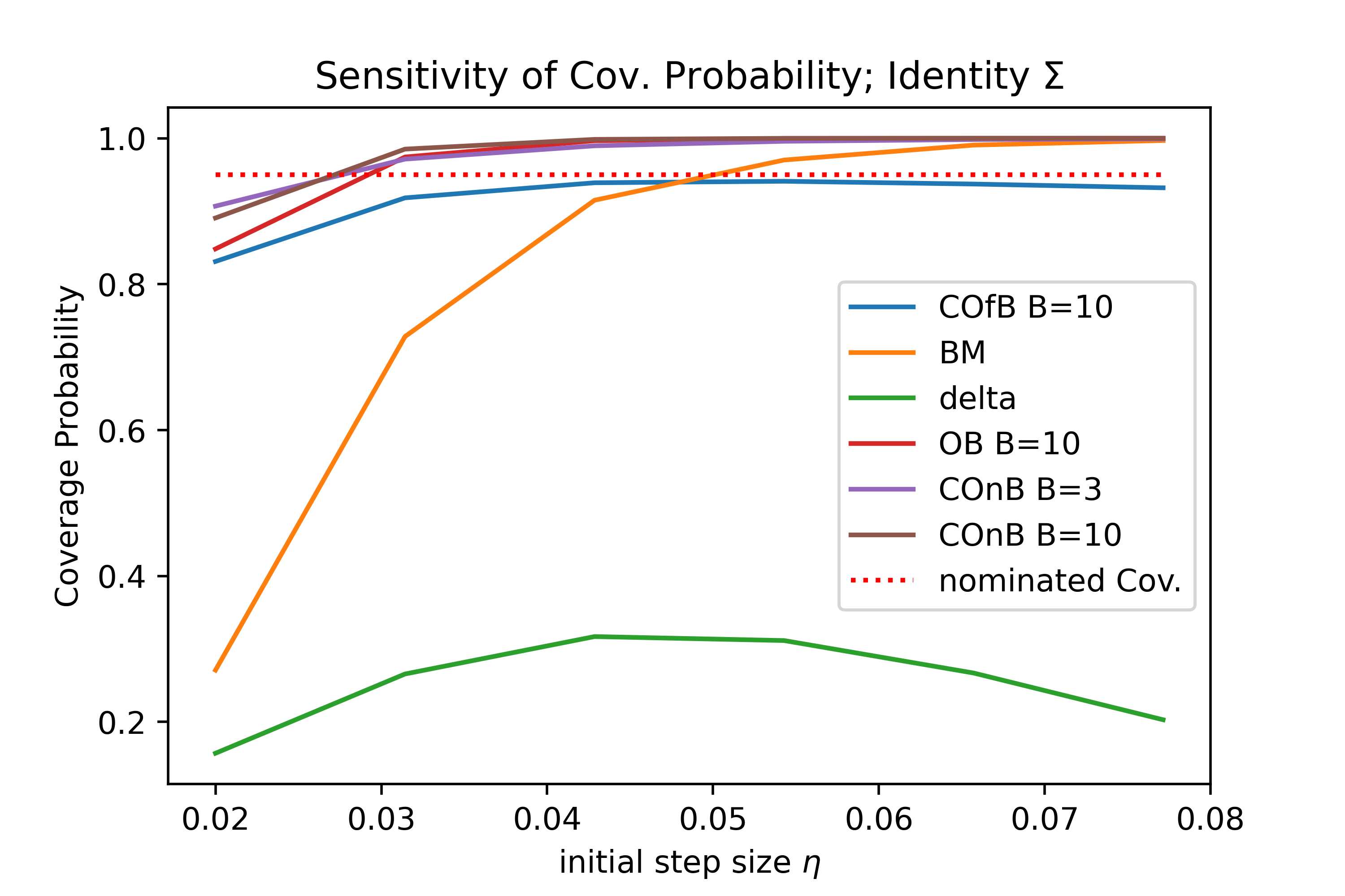
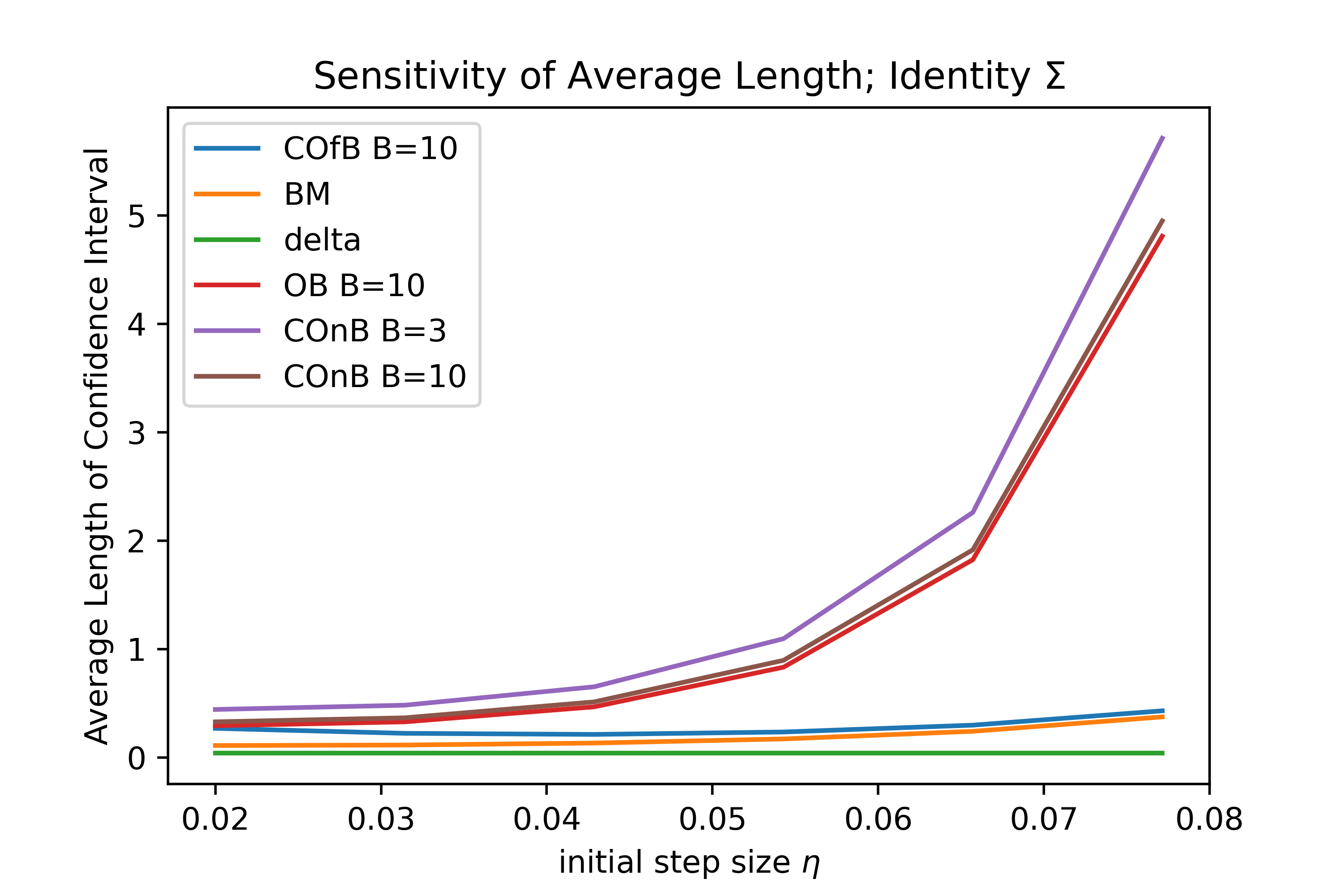
Figure 1: Performance of methods with respect to different choices of initial step size $\eta$, with sample size $n=10^{4}$. We compare the delta method, batch mean method with $M=n^{0.25}$, COfB method with $B=10$, COnB with $B=3,10$, and the online bootstrap method with $B=10$, when $n=10^{4}$. The left figure shows the sensitivity of the average coverage probability against $\eta$. The right figure shows the sensitivity of the average length of confidence interval against $\eta$. We report the result for identity $\Sigma$.

5.2 Baselines

In both experiments, we compare with the batch mean method and delta method in [7], the online bootstrap in [6], and the HiGrad method in [5].

The batch mean method splits $\{x_{i}\}_{i=0}^{n}$ into $M$ batches, where $M$ is an extra hyperparameter, with $e_{i}$ and $s_{i}$ denoting the ending index and starting index of the $i$-th batch respectively. $n_{k}$ denotes the number of iterates in $k$-th batch, and the estimator is defined to be $\frac{1}{M}\sum_{k=1}^{M}n_{k}(\bar{x}_{n_{k}}-\bar{x}_{M})(\bar{x}_{n_{k}}-\bar{x}_{M})^{\top}$, where $\bar{x}_{n_{k}}=\frac{1}{n_{k}}\sum_{i=s_{k}}^{e_{k}}x_{i}$ and $\bar{x}_{M}=\frac{1}{e_{M}-e{0}}\sum_{i=s_{1}}^{e_{M}}x_{i}$. Let $N=\frac{n^{1-\alpha}}{M+1}$, and $e_{k}$ to be the closest integer to $((k+1)N)^{\frac{1}{1-\alpha}}$ for each $k=0,\dots,M$ as suggested in [7]. The confidence interval for each entry of $\hat{x}$ is constructed using diagonal entries of the batch mean estimator and a normal quantile.

The delta method [7] generates confidence intervals using normal quantiles and $\tilde{\Sigma}_{n}^{2}=\tilde{G}_{n}^{-1}\tilde{S}_{n}\tilde{G}_{n}^{-1}$, where $\tilde{G}_{n}=\frac{1}{n}\sum_{i=1}^{n}\nabla^{2}h(x_{i-1},\zeta_{i})$, and $\tilde{S}_{n}=\frac{1}{n}\sum_{i=1}^{n}\nabla h(x_{i-1},\zeta_{i})(\nabla h(x_{i-1},\zeta_{i}))^{\top}$ are computed on the fly.

The online bootstrap method [6] runs $B+1$ ASGD threads in parallel. For each data $\zeta_{t}$, the update step for $b$-th thread is

$$x^{(b)}_{t}=x^{(b)}_{t-1}-\eta_{t}W^{(b)}_{t}\nabla h(x^{(b)}_{t-1},\zeta_{t}),\quad b=0,1,\dots,B$$

and $W^{(0)}_{t}=1,\ \forall t$. Then obtain $\{x^{(b)}\}_{b=0}^{B}$ by taking average along each thread of SGD. The sample variance for each coordinate $\sigma_{i},\ i=1,\dots,d$ is then calculated for $\{x^{(b)}\}_{b=1}^{B}$ with a known mean $x^{(0)}$. Then using normal quantile and $\sigma_{i}$, one can construct confidence intervals for each entry of $x^{*}$ centered at $x^{(0)}$.

The HiGrad method [5] takes two tuples $(B_{1},B_{2},\dots,B_{K})$ and $(n_{0},n_{1},\dots,n_{K})$ as hyperparameter describing when to break the SGD thread into how many branches. $B_{i}$ describes the number of branches a single branch divides into at $i$-th breaking. And $n_{i}$ describes the number of data each thread uses between $i$ and $i+1$-th breaking. After all the breaking, there will be $T=\prod_{i=1}^{K}B_{i}$ threads and one obtain $\{x^{(j)}\}_{j=1}^{\top}$ by averaging each thread. The confidence interval for $i$-th entry of $x^{*}$ is calculated by aggregating $\{x^{(j)}_{i}\}_{j=1}^{\top}$. It is worth pointing out that the total number of data used in HiGrad should be no more than $n$. i.e. $n_{0}+\sum_{i=1}^{K}B_{i}n_{i}\leq n$. Thus the length of a single thread in HiGrad is typically shorter than other methods discussed in this paper.

Method	delta	batch mean	OB ($B=100$)	$\text{HiGrid}_{(2,2)}$	COfB ASGD ($B=3$)	COnB ($B=3$)
Average Runtime (s)	$1.23$	$0.94$	$74.21$	$0.77$	$2.18$	$3.05$

Table 2: Average runtime for different methods for linear regression with $d=200$, identity $\Sigma$

5.3 Hyperparameters

The choices of hyperparameters in both experiments are listed here. The nominal coverage probability we consider is $95\%$. Dimension of the problem $d\in\{5,20,200\}$ and we report the result for three choices of covariance matrix $\Sigma$ of $a$. Namely, identity $\Sigma=I_{d}$, Toeplitz $\Sigma_{i,j}=0.5^{|i-j|}$ and equicorrelation case $\Sigma_{i,j}=0.2$ if $i\neq j$ and $\Sigma_{i,i}=1$. The decay rate for learning rate $\alpha=0.501$. The optimal solution $x^{*}=[0,\frac{1}{d-1},\frac{2}{d-1},\dots,1]^{\top}$ and we set the initial choice $x_{0}=[0,0,\dots,0]^{\top}$.

For each set of hyperparameters, we run 500 independent trials and report the mean and standard deviation of the coverage probabilities and the average length of the intervals across $d$ dimensions. We tune the initial step size $\eta$ within the range $[0.2,0.7]$ and report the result with the most accurate average coverage probability. For the batch mean method, $M$ is selected to be the nearest integer to $n^{0.25}$ as suggested in [7]. For HiGrad, the architecture we experiment on is $((2,2),(n/7,n/7,n/7))$. As mentioned in [5], this choice is desirable as it balances accuracy, coverage, and informativeness. We report the performance of COfB and COnB with $B=3,5,10$. For online bootstrap method, $B=200$ is the suggested choice in [6]. We also consider $B=10$ and $100$ based on the observation that online bootstrap with $B=100$ and $200$ perform similarly which prompts the question of whether smaller $B$’s would work.

5.4 Results

Results from linear and logistic regression experiments are presented in Tables 3 and 4, respectively. In these tables, bold numbers highlight favorable results, where the coverage probability lies between $92\%$ and $98\%$. Conversely, italic numbers indicate poor results, specifically those with coverage probabilities below $80\%$.

5.4.1 Coverage Probability

In terms of actual coverage probability for $d=5$ or $20$, the delta method, HiGrad method, and our approaches—irrespective of $B$—surpass both the batch mean method and the online bootstrap method with $B=10$. Our methodologies achieve an actual coverage rate of approximately $94-95\%$. In contrast, the batch mean method and online bootstrap with $B=10$ peak at about $92\%$.

Generally speaking, across all values of $d$ and $\Sigma$ considered in both experiments, the delta method and batch-mean method consistently fall behind other techniques. The HiGrad method displays a stark decline in performance at $d=200$, potentially attributed to its abbreviated SGD trajectory. Specifically, when $d=200$, the available data or iterations do not suffice for proper SGD convergence. Similarly, the performance of the delta method drops significantly as $d$ increases. This is largely due to its dependence on a Monte-Carlo estimation of a full Hessian matrix, the precision of which diminishes as dimensionality grows. In contrast, the merits of data reuse in bootstrap-type approaches become increasingly evident in higher dimensions. To this end, note that while the online bootstrap method yields comparable coverage probabilities, our methodologies are significantly faster.

5.4.2 Interval Width

In terms of the interval width, our approach does result in a longer average confidence interval relative to both the batch-mean method and the delta method. This outcome stems from the $t$-quantile with a degree of freedom defined by either $B-1$ for our COfB or $B$ for our COnB. However, given that entries of $x^{*}$ linearly span $[0,1]$ and the confidence intervals are of magnitude $10^{-2}$, the computational advantages seem to more than compensate for the modest increase in interval length.

5.4.3 Execution Time

Running times for the linear regression experiments across varied methodologies are available in Table 2. These experiments were conducted on a single 3.4GHz processor. Both HiGrad and the batch mean method emerged as the swiftest, attributed to their avoidance of additional gradient steps or Hessian calculations. Broadly, computation times align proportionately with the number of gradient steps except for the delta method. Both our methods take roughly three times longer than HiGrid, while the online bootstrap with $B=100$ takes around 100 times as long as HiGrid. One might also notice that COnB has a slightly longer runtime compared to COfB, which is due to the additional computational effort required to generate $\{W_{b,t}\}$.

5.4.4 Sensitivity Analysis

In Figure 1, we compare the performance of our methods, the delta method, the batch mean method, and the online bootstrap method with the number of samples $n=10^{4}$ for the linear regression problem. Observe that the coverage probability of COfB methods remains stable around $95\%$ regardless of changes in the initial step size. On the other hand, the batch mean method requires a careful choice of the initial step size to give a comparable coverage rate, and the optimal choice is not the same across different problems. The delta method suffers from a huge under-coverage and fails to give a valid confidence interval. The delta method and the batch mean method have smaller average lengths, which can be associated with their under-coverages. It can be observed that the coverage probability and the average length of the batch mean estimator both increase as $\eta$ increases. Our COnB method has a similar sensitivity as the online bootstrap method. Nonetheless, as mentioned earlier, COnB is substantially faster. Additionally, the average length of our COnB becomes almost the same as that of the online bootstrap method when increasing $B$ to $10$.

Identity $\Sigma$, $n=10^{5}$
	$d=5$		$d=20$		$d=200$
	Cov (%)	Len ($\times 10^{-2}$)	Cov (%)	Len ($\times 10^{-2}$)	Cov (%)	Len ($\times 10^{-2}$)
delta	94.84 ($0.07$)	$1.24$ ($0.00$)	94.38 ($0.07$)	$1.24$ ($0.00$)	71.37 ($0.14$)	$1.24$ ($0.00$)
BM	92.72 ($0.08$)	$1.23$ ($0.00$)	92.92 ($0.08$)	$1.29$ ($0.00$)	$98.34$ ($0.04$)	$3.65$ ($0.00$)
OB $B=10$	92.36 ($0.08$)	$1.26$ ($0.00$)	92.42 ($0.08$)	$1.26$ ($0.00$)	$99.78$ ($0.05$)	$6.43$ ($0.01$)
OB $B=100$	94.88 ($0.07$)	$1.29$ ($0.00$)	95.16 ($0.07$)	$1.29$ ($0.00$)	$100.00$ ($0.00$)	$7.30$ ($0.01$)
$\text{HiGrad}_{(2,2)}$	95.67 ($0.06$)	$2.56$ ($0.01$)	95.29 ($0.07$)	$2.66$ ($0.01$)	96.03 ($0.06$)	$2.67$ ($0.01$)
COfB ASGD $B=3$	95.44 ($0.07$)	$2.44$ ($0.00$)	94.49 ($0.07$)	$2.46$ ($0.00$)	92.31 ($0.08$)	$20.71$ ($16.16$)
COfB ASGD $B=5$	95.24 ($0.07$)	$1.68$ ($0.00$)	94.55 ($0.07$)	$1.69$ ($0.00$)	94.59 ($0.07$)	$3.06$ ($1.18$)
COfB ASGD $B=10$	95.04 ($0.07$)	${1.40}$ ($0.00$)	94.82 ($0.07$)	${1.42}$ ($0.00$)	94.30 ($0.07$)	$2.56$ ($0.00$)
COfB SGD $B=3$	94.96 ($0.07$)	$3.16$ ($0.00$)	94.53 ($0.07$)	$3.18$ ($0.00$)	94.59 ($0.07$)	$3.20$ ($0.00$)
COfB SGD $B=5$	94.44 ($0.07$)	$2.17$ ($0.00$)	94.30 ($0.07$)	$2.17$ ($0.00$)	94.42 ($0.07$)	$2.19$ ($0.00$)
COfB SGD $B=10$	94.68 ($0.07$)	$1.82$ ($0.00$)	93.97 ($0.08$)	$1.83$ ($0.00$)	94.33 ($0.07$)	${1.84}$ ($0.00$)
COnB $B=3$	95.32 ($0.07$)	$1.94$ ($0.00$)	94.63 ($0.07$)	$1.97$ ($0.00$)	$99.17$ ($0.03$)	$9.15$ ($0.02$)
COnB $B=5$	95.04 ($0.07$)	$1.61$ ($0.00$)	95.06 ($0.07$)	$1.61$ ($0.00$)	$99.62$ ($0.02$)	$8.02$ ($0.01$)
COnB $B=10$	95.16 ($0.07$)	$1.40$ ($0.00$)	95.52 ($0.07$)	$1.43$ ($0.00$)	$99.88$ ($0.01$)	$7.31$ ($0.01$)
Toeplitz $\Sigma$, $n=10^{5}$
delta	94.20 ($0.07$)	$1.53$ ($0.00$)	93.23 ($0.08$)	$1.58$ ($0.00$)	37.16 ($0.15$)	$1.60$ ($0.00$)
BM	$91.80$ ($0.09$)	$1.53$ ($0.00$)	$88.51$ ($0.10$)	$1.51$ ($0.00$)	97.37 ($0.05$)	$6.54$ ($0.01$)
OB $B=10$	92.48 ($0.08$)	$1.66$ ($0.00$)	93.68 ($0.08$)	$1.81$ ($0.00$)	93.33 ($0.25$)	$13.73$ ($0.01$)
OB $B=100$	95.48 ($0.07$)	$1.72$ ($0.00$)	95.84 ($0.06$)	$1.97$ ($0.00$)	96.58 ($0.18$)	$14.26$ ($0.01$)
$\text{HiGrad}_{(2,2)}$	94.33 ($0.07$)	$2.69$ ($0.01$)	94.88 ($0.07$)	$2.82$ ($0.01$)	94.09 ($0.07$)	$2.83$ ($0.01$)
COfB ASGD $B=3$	94.72 ($0.07$)	$3.06$ ($0.00$)	94.95 ($0.07$)	$3.30$ ($0.00$)	94.41 ($0.07$)	$14.44$ ($0.02$)
COfB ASGD $B=5$	95.24 ($0.07$)	$2.21$ ($0.00$)	94.89 ($0.07$)	$2.26$ ($0.00$)	93.91 ($0.08$)	$9.96$ ($0.01$)
COfB ASGD $B=10$	95.28 ($0.07$)	${1.74}$ ($0.00$)	94.95 ($0.07$)	${2.12}$ ($0.00$)	94.01 ($0.08$)	$8.44$ ($0.01$)
COfB SGD $B=3$	95.16 ($0.07$)	$6.93$ ($0.01$)	94.76 ($0.07$)	$4.34$ ($0.00$)	95.16 ($0.07$)	$6.90$ ($0.01$)
COfB SGD $B=5$	95.84 ($0.06$)	$4.70$ ($0.00$)	94.20 ($0.07$)	$2.97$ ($0.00$)	95.04 ($0.07$)	$4.72$ ($0.00$)
COfB SGD $B=10$	95.36 ($0.07$)	$3.95$ ($0.00$)	94.20 ($0.07$)	$2.50$ ($0.00$)	95.00 ($0.07$)	${3.98}$ ($0.00$)
COnB $B=3$	95.00 ($0.07$)	$2.49$ ($0.00$)	95.36 ($0.07$)	$2.94$ ($0.00$)	95.41 ($0.07$)	$21.04$ ($0.02$)
COnB $B=5$	94.60 ($0.07$)	$1.96$ ($0.00$)	95.43 ($0.07$)	$2.44$ ($0.00$)	95.48 ($0.07$)	$17.42$ ($0.02$)
COnB $B=10$	94.92 ($0.07$)	$1.77$ ($0.00$)	95.42 ($0.07$)	$2.18$ ($0.00$)	95.78 ($0.06$)	$15.61$ ($0.01$)
equicorrelation $\Sigma$, $n=10^{5}$
delta	94.76 ($0.07$)	$1.31$ ($0.00$)	93.94 ($0.08$)	$1.36$ ($0.00$)	25.95 ($0.14$)	$1.38$ ($0.00$)
BM	93.20 ($0.08$)	$1.30$ ($0.00$)	92.10 ($0.09$)	$1.44$ ($0.00$)	$99.74$ ($0.02$)	$34.65$ ($0.22$)
OB $B=10$	92.88 ($0.08$)	$1.35$ ($0.00$)	92.78 ($0.08$)	$1.45$ ($0.00$)	$89.23$ ($0.31$)	$19.42$ ($0.04$)
OB $B=100$	95.28 ($0.07$)	$1.39$ ($0.00$)	94.73 ($0.07$)	$1.52$ ($0.00$)	94.29 ($0.23$)	$20.78$ ($0.03$)
$\text{HiGrad}_{(2,2)}$	95.00 ($0.07$)	$2.59$ ($0.01$)	95.12 ($0.07$)	$2.78$ ($0.01$)	95.93 ($0.06$)	$2.83$ ($0.01$)
COfB ASGD $B=3$	94.76 ($0.07$)	$2.58$ ($0.00$)	94.66 ($0.07$)	$2.74$ ($0.00$)	93.23 ($0.08$)	$32.56$ ($0.04$)
COfB ASGD $B=5$	95.52 ($0.07$)	$1.77$ ($0.00$)	95.02 ($0.07$)	$1.88$ ($0.00$)	$90.80$ ($0.09$)	$52.72$ ($0.29$)
COfB ASGD $B=10$	95.44 ($0.07$)	${1.48}$ ($0.00$)	94.95 ($0.07$)	${1.58}$ ($0.00$)	$91.87$ ($0.09$)	$49.84$ ($0.22$)
COfB SGD $B=3$	93.28 ($0.08$)	$3.19$ ($0.00$)	93.85 ($0.08$)	$3.26$ ($0.00$)	94.53 ($0.07$)	${4.43}$ ($0.00$)
COfB SGD $B=5$	93.16 ($0.08$)	$2.18$ ($0.00$)	93.45 ($0.08$)	$2.23$ ($0.00$)	94.20 ($0.07$)	$3.06$ ($0.00$)
COfB SGD $B=10$	95.20 ($0.07$)	$3.94$ ($0.00$)	94.78 ($0.07$)	$3.94$ ($0.00$)	94.08 ($0.07$)	$2.57$ ($0.00$)
COnB $B=3$	95.16 ($0.07$)	$2.05$ ($0.00$)	95.00 ($0.07$)	$2.28$ ($0.00$)	92.55 ($0.08$)	$31.28$ ($0.16$)
COnB $B=5$	95.16 ($0.07$)	$1.65$ ($0.00$)	94.60 ($0.07$)	$1.89$ ($0.00$)	92.26 ($0.08$)	$23.83$ ($0.04$)
COnB $B=10$	95.60 ($0.06$)	$1.48$ ($0.00$)	95.07 ($0.07$)	$1.68$ ($0.00$)	92.54 ($0.08$)	$22.08$ ($0.04$)

Table 3: Results for the linear regression experiment

Identity $\Sigma$, $n=10^{5}$
	$d=5$		$d=20$		$d=200$
	Cov (%)	Len ($\times 10^{-2}$)	Cov (%)	Len ($\times 10^{-2}$)	Cov (%)	Len ($\times 10^{-2}$)
delta	95.00 ($0.07$)	$3.10$ ($0.00$)	94.12 ($0.07$)	$3.68$ ($0.00$)	61.92 ($0.15$)	$5.85$ ($0.00$)
BM	$89.33$ ($0.10$)	$2.64$ ($0.00$)	$87.29$ ($0.11$)	$3.11$ ($0.01$)	57.47 ($0.16$)	$5.56$ ($0.02$)
OB ($B=100$)	95.00 ($0.07$)	$3.21$ ($0.00$)	96.71 ($0.06$)	$4.34$ ($0.01$)	$99.88$ ($0.01$)	$50.95$ ($0.23$)
OB ($B=200$)	94.83 ($0.07$)	$3.18$ ($0.00$)	96.96 ($0.05$)	$4.41$ ($0.01$)	$99.91$ ($0.01$)	$50.71$ ($0.23$)
$\text{HiGrad}_{(2,2)}$	94.33 ($0.07$)	$5.77$ ($0.02$)	95.46 ($0.07$)	$7.10$ ($0.02$)	$80.61$ ($0.13$)	$10.26$ ($0.04$)
COfB ASGD $B=3$	94.12 ($0.07$)	$4.21$ ($0.00$)	95.03 ($0.07$)	$7.32$ ($0.01$)	92.34 ($0.08$)	$19.00$ ($0.02$)
COfB ASGD $B=5$	95.08 ($0.07$)	$4.14$ ($0.00$)	94.77 ($0.07$)	$5.01$ ($0.00$)	$90.64$ ($0.09$)	$13.03$ ($0.01$)
COfB ASGD $B=10$	94.88 ($0.07$)	$3.52$ ($0.00$)	94.51 ($0.07$)	$4.22$ ($0.00$)	$89.37$ ($0.10$)	$11.06$ ($0.01$)
COfB SGD $B=3$	95.40 ($0.07$)	$9.38$ ($0.01$)	94.99 ($0.07$)	$9.42$ ($0.01$)	94.72 ($0.07$)	$25.61$ ($0.03$)
COfB SGD $B=5$	95.44 ($0.07$)	$7.93$ ($0.00$)	94.70 ($0.07$)	$7.93$ ($0.00$)	94.66 ($0.07$)	$17.57$ ($0.01$)
COfB SGD $B=10$	95.44 ($0.07$)	$7.93$ ($0.00$)	94.70 ($0.07$)	$7.93$ ($0.00$)	94.54 ($0.07$)	$14.84$ ($0.01$)
COnB ($B=3$)	94.33 ($0.07$)	$4.71$ ($0.02$)	95.62 ($0.06$)	$6.56$ ($0.03$)	$99.42$ ($0.02$)	$75.25$ ($0.43$)
COnB ($B=5$)	95.33 ($0.07$)	$3.93$ ($0.01$)	96.79 ($0.06$)	$5.35$ ($0.02$)	$99.50$ ($0.02$)	$64.17$ ($0.35$)
COnB ($B=10$)	94.83 ($0.07$)	$3.55$ ($0.01$)	97.00 ($0.05$)	$4.85$ ($0.01$)	$99.72$ ($0.02$)	$57.67$ ($0.30$)
Toeplitz $\Sigma$, $n=10^{5}$
delta	94.83 ($0.07$)	$4.05$ ($0.00$)	93.29 ($0.08$)	$5.59$ ($0.00$)	53.69 ($0.16$)	$9.56$ ($0.00$)
BM	$84.00$ ($0.12$)	$3.16$ ($0.01$)	75.25 ($0.14$)	$3.75$ ($0.01$)	34.93 ($0.15$)	$7.30$ ($0.03$)
OB ($B=100$)	95.00 ($0.07$)	$4.22$ ($0.00$)	94.04 ($0.07$)	$6.65$ ($0.01$)	$99.78$ ($0.01$)	$69.55$ ($0.26$)
OB ($B=200$)	95.00 ($0.07$)	$4.24$ ($0.00$)	94.67 ($0.07$)	$6.70$ ($0.01$)	$99.78$ ($0.01$)	$69.28$ ($0.26$)
$\text{HiGrad}_{(2,2)}$	95.33 ($0.07$)	$7.18$ ($0.03$)	93.38 ($0.08$)	$8.92$ ($0.03$)	57.02 ($0.16$)	$10.27$ ($0.04$)
COfB ASGD $B=3$	94.12 ($0.07$)	$5.70$ ($0.00$)	94.77 ($0.07$)	$11.49$ ($0.01$)	93.79 ($0.08$)	$42.27$ ($0.05$)
COfB ASGD $B=5$	94.32 ($0.07$)	$4.82$ ($0.00$)	94.81 ($0.07$)	$7.97$ ($0.01$)	93.23 ($0.08$)	$28.81$ ($0.02$)
COfB ASGD $B=10$	94.88 ($0.07$)	$4.61$ ($0.00$)	94.65 ($0.07$)	$6.69$ ($0.00$)	93.09 ($0.08$)	$24.43$ ($0.01$)
COfB SGD $B=3$	95.36 ($0.07$)	$9.48$ ($0.01$)	94.80 ($0.07$)	$9.65$ ($0.01$)	94.41 ($0.07$)	$30.53$ ($0.03$)
COfB SGD $B=5$	95.40 ($0.07$)	$7.98$ ($0.00$)	94.37 ($0.07$)	$8.16$ ($0.00$)	93.79 ($0.08$)	$20.76$ ($0.02$)
COfB SGD $B=10$	95.40 ($0.07$)	$7.98$ ($0.00$)	94.37 ($0.07$)	$8.16$ ($0.00$)	93.62 ($0.08$)	$17.56$ ($0.01$)
COnB ($B=3$)	94.00 ($0.08$)	$6.22$ ($0.02$)	94.71 ($0.07$)	$10.27$ ($0.05$)	97.82 ($0.05$)	$99.61$ ($0.60$)
COnB ($B=5$)	95.00 ($0.07$)	$5.25$ ($0.02$)	94.71 ($0.07$)	$8.20$ ($0.03$)	$98.75$ ($0.04$)	$85.15$ ($0.45$)
COnB ($B=10$)	94.83 ($0.07$)	$4.84$ ($0.01$)	94.29 ($0.07$)	$7.25$ ($0.02$)	$99.31$ ($0.03$)	$78.02$ ($0.37$)
equicorrelation $\Sigma$, $n=10^{5}$
delta	94.83 ($0.07$)	$3.39$ ($0.00$)	94.12 ($0.07$)	$5.19$ ($0.00$)	31.55 ($0.15$)	$13.50$ ($0.01$)
BM	$90.00$ ($0.09$)	$2.92$ ($0.00$)	$81.25$ ($0.12$)	$3.84$ ($0.01$)	14.67 ($0.11$)	$7.17$ ($0.03$)
OB ($B=100$)	95.00 ($0.07$)	$3.50$ ($0.00$)	95.46 ($0.07$)	$6.37$ ($0.02$)	$98.12$ ($0.04$)	$110.74$ ($0.42$)
OB ($B=200$)	94.67 ($0.07$)	$3.50$ ($0.00$)	95.92 ($0.06$)	$6.42$ ($0.02$)	$98.38$ ($0.04$)	$109.89$ ($0.40$)
$\text{HiGrad}_{(2,2)}$	96.17 ($0.06$)	$5.97$ ($0.02$)	95.00 ($0.07$)	$9.11$ ($0.03$)	26.94 ($0.14$)	$11.30$ ($0.04$)
COfB ASGD $B=3$	94.12 ($0.07$)	$4.68$ ($0.00$)	94.87 ($0.07$)	$10.42$ ($0.01$)	$83.65$ ($0.12$)	$64.61$ ($0.08$)
COfB ASGD $B=5$	93.96 ($0.08$)	$3.92$ ($0.00$)	94.96 ($0.07$)	$7.11$ ($0.01$)	76.52 ($0.13$)	$44.29$ ($0.04$)
COfB ASGD $B=10$	95.12 ($0.07$)	$3.85$ ($0.00$)	94.78 ($0.07$)	$6.04$ ($0.00$)	71.44 ($0.14$)	$37.42$ ($0.02$)
COfB SGD $B=3$	94.96 ($0.07$)	$9.39$ ($0.01$)	93.85 ($0.08$)	$9.50$ ($0.01$)	77.71 ($0.13$)	$39.47$ ($0.05$)
COfB SGD $B=5$	94.76 ($0.07$)	$7.92$ ($0.00$)	93.59 ($0.08$)	$8.06$ ($0.00$)	66.67 ($0.15$)	$26.98$ ($0.03$)
COfB SGD $B=10$	94.76 ($0.07$)	$7.92$ ($0.00$)	93.59 ($0.08$)	$8.06$ ($0.00$)	58.94 ($0.16$)	$22.78$ ($0.02$)
COnB ($B=3$)	94.17 ($0.07$)	$5.18$ ($0.02$)	95.96 ($0.06$)	$9.51$ ($0.06$)	93.07 ($0.08$)	$138.99$ ($1.13$)
COnB ($B=5$)	94.67 ($0.07$)	$4.38$ ($0.01$)	95.12 ($0.07$)	$7.66$ ($0.03$)	94.14 ($0.07$)	$115.73$ ($0.73$)
COnB ($B=10$)	95.00 ($0.07$)	$3.94$ ($0.01$)	95.83 ($0.06$)	$6.92$ ($0.02$)	95.90 ($0.06$)	$111.29$ ($0.60$)

Table 4: Results for the logistic regression experiment

6 Conclusion

In this work, we examined the challenges in existing SGD inference techniques, which include issues related to hyperparameter tuning, substantial modifications to the original SGD algorithm, and considerable computational and storage demands. Motivated by these challenges, we presented two resampling-based methods to quantify uncertainty in (A)SGD where, unlike in the classical bootstrap, the number of resampled (A)SGD trajectories can be very small (as low as 1 or 2) while asymptotic coverage-exactness is still attained. Our methods arguably circumvent the need for hyper-parameter tuning or substantial modification to the SGD procedure by inheriting the advantages of the bootstrap, but incur only a modest increase in computational overhead thanks to the few resampled trajectories. Theoretically, our methods can be viewed as enhancements of the classical bootstrap and existing online bootstrap by leveraging the recent so-called cheap bootstrap idea, which allows running very few bootstrap replications via the use of asymptotic sample-resample independence. Towards this, we derived the joint central limit of (A)SGD and resampled (A)SGD via a generalization of recent Berry-Esseen-type results. Finally, we compared our methods empirically against benchmark approaches on various regression problems and showcased some encouraging performances.

Appendix A Useful Lemmas and Missing Proofs

A.1 Convergence of Normal Variables with Empirical Variances

We first show the following:

Lemma 12.

Under the same assumptions as Theorem 7, let $g:\mathbb{R}\rightarrow\mathbb{R}$ be any bounded continuous function. We have

$$\mathbb{E}^{*}[g(\hat{Z}_{n})]\rightarrow\mathbb{E}[g(Z)]\quad\text{in probability}$$ (15)

where $\mathbb{E}^{*}$ denotes the expectation conditional on data.

Proof.

Recall that $\hat{Z}_{n}$ has distribution the same as the weak limit of $\sqrt{m}(\psi_{m}(\hat{P}_{n})-\psi(\hat{P}_{n}))$ conditional on $\hat{P}_{n}$. Let $\sigma_{n}^{2}$ and $\sigma^{2}$ denote the variance of $\hat{Z}_{n}$ and $Z$ respectively. In other words, $\hat{Z}_{n}\sim N(0,\sigma_{n}^{2})$ and $Z\sim N(0,\sigma^{2})$.

By definition, $\mathbb{E}^{*}[g(\hat{Z}_{n})]=\int g(x)p(x;0,\sigma_{n}^{2})dx$ where $p(x;0,\sigma_{n}^{2})$ denotes the probability density function of the multivariate normal distribution with mean $0$ covariance matrix $\sigma_{n}^{2}$ evaluated at $x$. Observe that $\mathbb{E}^{*}[g(\hat{Z}_{n})]$ is continuous as a function of $\sigma_{n}$. Since convergence in probability is preserved by continuous functions, it suffices to prove that $\sigma_{n}^{2}\rightarrow\sigma^{2}$ in probability.

Consider the ASGD case now, and the SGD case can be treated similarly. Recall that $\sigma_{n}^{2}=G_{n}(\hat{x}_{n})^{-1}S_{n}(\hat{x}_{n})G_{n}(\hat{x}_{n})^{-1}$ and $\sigma^{2}=G(x^{*})^{-1}S(x^{*})G(x^{*})^{-1}$. Again by continuity, to prove that $\sigma_{n}^{2}\rightarrow\sigma^{2}$, it suffices to show that each entry of $G_{n}(\hat{x}_{n})$ and $S_{n}(\hat{x}_{n})$ converges to $G(x^{*})$ and $S(x^{*})$ in probability respectively.

Claim 1: Fix any $i,j\in 1,\dots,d$, we have

$$(G_{n}(\hat{x}_{n}))_{i,j}\rightarrow(G(x^{*}))_{i,j}\ \text{in probability}$$ (16)

Recall the definition of $G_{n}$ and $G$, we have

$$(G_{n}(\hat{x}_{n}))_{i,j}=\frac{1}{n}\sum_{t=1}^{n}\partial^{2}_{i,j}h(\hat{x}_{n},\zeta_{t})\quad\text{ and }\quad(G(x^{*}))_{i,j}=\int\partial^{2}_{i,j}h(x^{*},\zeta)P(d\zeta)$$

To simplify the notation, we write $Qf(x)\triangleq\int f(x,\zeta)Q(d\zeta)$ for a function $f$ parameterized by $x$ and a probability measure $Q$. Then, $(G_{n}(\hat{x}_{n}))_{i,j}=\hat{P}_{n}\partial^{2}_{i,j}h(\hat{x}_{n})$ and $(G(x^{*}))_{i,j}=P\partial^{2}_{i,j}h(x^{*})$.

Recall that $\mathcal{F}_{i,j}=\{\partial^{2}_{i,j}h(x,\zeta):x\in\mathcal{X}\}$, which is parameterized by the bounded set $\mathcal{X}$. By assumption, $\mathcal{F}_{i,j}$ is $P$-Glivenko-Cantelli (see, Example 19.8 in [27]) and we have

$$\sup_{f\in\mathcal{F}}|\hat{P}_{n}f-Pf|\xrightarrow{as*}0$$ (17)

And we have the following

$$\begin{split}&(G_{n}(\hat{x}_{n}))_{i,j}-(G(x^{*}))_{i,j}\\ =&(\hat{P}_{n}\partial^{2}_{i,j}h(\hat{x}_{n})-P\partial^{2}_{i,j}h(\hat{x}^{n}))\textbf{1}\{\hat{x}\in\mathcal{X}\}\\ &+(\hat{P}_{n}\partial^{2}_{i,j}h(\hat{x}_{n})-P\partial^{2}_{i,j}h(\hat{x}_{n}))\textbf{1}\{\hat{x}\notin\mathcal{X}\}+(P\partial^{2}_{i,j}h(\hat{x}_{n})-P\partial^{2}_{i,j}h(x^{*}))\end{split}$$ (18)

By (17), $(\hat{P}_{n}\partial^{2}_{i,j}h(\hat{x}_{n})-P\partial^{2}_{i,j}h(\hat{x}^{n}))\textbf{1}\{\hat{x}\in\mathcal{X}\}\xrightarrow{P}0$. Using the fact that $\hat{x}_{n}\xrightarrow{P}x^{*}$ and by continuous mapping Theorem, the second and the last term on the right-hand side of (18) also converges to $0$ in probability. So we finish the proof of our first claim.

Claim 2: Fix any $i,j\in 1,\dots,d$, we have

$$(S_{n}(\hat{x}_{n}))_{i,j}\rightarrow(S(x^{*}))_{i,j}\ \text{in probability}$$ (19)

By definition, $(S_{n}(\hat{x}_{n}))_{i,j}=\hat{P}_{n}\partial_{i}h(\hat{x}_{n})\partial_{j}h(\hat{x}_{n})$ and $(S(x^{*}))_{i,j}=P\partial_{i}h(x^{*})\partial_{j}h(x^{*})$. Define $\mathcal{F}=\{\partial_{i}h(x,\zeta)\partial_{j}h(x,\zeta):x\in\mathcal{X}\}$. And notice that $\mathcal{F}$ is $P$-Glivenko-Cantelli. The remaining proof follows the same arguments as in the proof of the first claim.

As a result, $\sigma_{n}^{2}\xrightarrow{P}\sigma^{2}$. And we conclude that $\mathbb{E}^{*}[g(\hat{Z}_{n})]\rightarrow\mathbb{E}[g(Z)]$ in probability. ∎

We then have the following convergence result:

Lemma 13.

Under the same assumptions as Theorem 7, for any Borel set $D$,

$$|\mathbb{P}^{*}(\hat{Z}_{n}\in D)-\mathbb{P}(Z_{0}\in D)|\rightarrow 0\quad\text{in probability}$$

Proof.

Let $D_{1}$, and $D_{2}$ denote the interior and closure of $D$ respectively. Consider $g_{m}(\cdot)=\min(1,md(x,D_{1}^{c}))$, for $m=1,2,\dots$. Then, by Lemma 12, for fixed $m$,

$$\mathbb{E}^{*}[g_{m}(\hat{Z}_{n})]\rightarrow\mathbb{E}[g_{m}(Z)]\quad\text{in probability}$$

Also, for fixed $m$, by the above relationship and monotone convergence theorem,

$$\liminf_{n\rightarrow\infty}\mathbb{P}^{*}(\hat{Z}_{n}\in D_{1})\geq\liminf_{n\rightarrow\infty}\mathbb{E}^{*}[g_{m}(\hat{Z}_{n})]=\mathbb{E}[g_{m}(Z)]\xrightarrow{m\rightarrow\infty}\mathbb{P}(Z_{0}\in D_{1})=\mathbb{P}(Z_{0}\in D)$$

By considering the complement of $D_{2}$, and $\bar{g}_{m}=\min(1,md(x,D_{2}))$, we obtain the opposite side of the above inequality. And the desired result follows. ∎

A.2 A Useful Berry-Esseen-Type Bound

Lemma 14.

[25] Let $T$ be a d-dimensional statistics. Suppose that $T=T(\zeta_{1},\dots,\zeta_{n})$ admits the decomposition $T=W+D$, such that $W=\sum_{i=1}^{n}f_{i}(\zeta_{i})$ satisfies

$$\mathbb{E}[f_{i}(\zeta_{i})]=0,\forall i\quad\text{and }\sum_{i=1}^{n}\mathbb{E}[f_{i}(\zeta_{i})(f_{i}(\zeta_{i}))^{\top}]=\Sigma_{n}$$

with $0<\sigma_{n}=\lambda_{min}(\Sigma_{n})$ and $f$ is some mapping to $\mathbb{R}^{d}$. Define $\gamma_{n}=\sum_{i=1}^{n}\mathbb{E}\|f_{i}(\zeta_{i})\|^{3}$. And let $\Delta$ and $(\Delta^{(i)}){1\leq i\leq n}$ be random variables such that $\Delta\geq\|D\|$ and $\Delta^{(i)}$ is independent of $\zeta_{i}$. Let $Z_{0}\sim\mathcal{N}(0,I_{d})$ Then,

$$\sup_{A}|\mathbb{P}(\Sigma_{n}^{-1/2}T\in A)-\mathbb{P}(Z_{0}\in A)|$$

$$\leq \ 259\sigma_{n}^{-3/2}d^{1/2}\gamma_{n}+2\sigma_{n}^{-1}\mathbb{E}[\|W\|\Delta]+2\sigma_{n}^{-1}\sum_{i=1}^{n}\mathbb{E}[\|f_{i}(\zeta_{i})\||\Delta-\Delta^{(i)}|]$$

A.3 Proof of Theorem 8 in the ASGD Case

It suffices show: there is a 4-tuple $(\hat{\tau_{0}},\hat{\tau},\hat{C},N)$ such that

$$\sup_{n>N}|\mathbb{P}^{*}(\sqrt{n}(\psi_{n}(\hat{P}_{n})-\hat{\psi}(\hat{P}_{n}))\in D)-\mathbb{P}(\sigma(\hat{P}_{n})\in D)|\leq\hat{C}(d^{3/2}+\hat{\tau}^{3}+\hat{\tau}_{0}^{3})(d^{1/2}n^{-1/2}+n^{-\alpha+1/2})$$ (20)

for any measurable $D$.

[25] put forward the following bound

$$\begin{split}|\mathbb{P}(\sqrt{n}(\psi_{n}(P)-\hat{\psi}(P))\in D)-\mathbb{P}(Z\in D)|\leq C(d^{3/2}+\tau^{3}+\tau_{0}^{3})(d^{1/2}n^{-1/2}+n^{-\alpha+1/2})\end{split}$$ (21)

where $C=C(\eta,\lambda_{1},\lambda_{2},\alpha,l,L)>0$ is a constant independent of $D$, $d$, $\tau$, and $\tau_{0}$.

Discuss $\hat{\tau}_{0}$ first. Let $\epsilon>0$. Consider $\hat{\tau_{0}}=(1+\epsilon)\tau_{0}$, by assumptions 1 and 4, we have the consistency of estimator $\hat{\psi}(\hat{P}_{n})$. Namely, $\hat{\psi}(\hat{P}_{n})\xrightarrow{P}\hat{\psi}(P)$. [27] As a result, except possibly for a Null set, there is $N=N(\epsilon)$ such that for any $n>N$, we have $\|\hat{\psi}(P)-\hat{\psi}(\hat{P}_{n})\|<\tau_{0}$. So $\|x_{0}-\hat{\psi}(\hat{P}_{n})\|\leq\|x_{0}-\hat{\psi}(P)\|+\|\hat{\psi}(P)-\hat{\psi}(\hat{P}_{n})\|\leq(1+\epsilon)\tau_{0}=\hat{\tau}_{0}$ almost surely.

For $\hat{\tau}$, notice that we have for any $n>N$

$$\|\nabla h(\hat{\psi}(\hat{P}_{n}),\hat{\zeta})\|_{4} \leq\|\nabla h(\hat{\psi}(P),\hat{\zeta})\|_{4}+\|\nabla h(\hat{\psi}(P),\hat{\zeta})-\nabla h(\hat{\psi}(\hat{P}_{n}),\hat{\zeta})\|_{4}$$

$$\leq\|\nabla h(\hat{\psi}(P),\hat{\zeta})\|_{4}+L\tau_{0}$$

where $\hat{\zeta}\sim\hat{P}_{n}$. By the law of large numbers, for the first term, we have

$$\|\nabla h(\hat{\psi}(P),\hat{\zeta})\|_{4}\xrightarrow{n\rightarrow\infty}\|\nabla h(\hat{\psi}(P),\zeta)\|_{4}\leq\tau_{0}$$

As a result, $\|\nabla h(\hat{\psi}(P),\hat{\zeta})\|_{4}$ is bounded by a constant, uniformly in $n$. So we conclude that there exist such $\hat{\tau}$ that $\|\nabla h(\hat{\psi}(\hat{P}_{n}),\hat{\zeta})\|_{4}\leq\hat{\tau}$ for all $n>N$.

To determine $\hat{C}$, it suffices to show find $\hat{\lambda_{1}},\hat{\lambda_{2}},\hat{l}$ and $\hat{L}$, since $\hat{\alpha}$ and $\eta$ are not affected by the underlying data distribution $P$.

For $\hat{\lambda_{1}}$ and $\hat{\lambda}_{2}$, recall that $S(x)\triangleq\mathbb{E}_{\zeta\sim P}[\nabla h(x,\zeta)(\nabla h(x,\zeta))^{\top}]$ and $S_{n}(x)\triangleq\mathbb{E}_{\hat{\zeta}\sim\hat{P}_{n}}[\nabla h(x,\hat{\zeta})(\nabla h(x,\hat{\zeta}))^{\top}]$. We have

$$\|(S_{n}(\hat{\psi}(\hat{P}_{n}))-S(x^{*}))\|\leq\|(S_{n}(\hat{\psi}(\hat{P}_{n}))-S_{n}(x^{*}))\|+\|(S_{n}(x^{*})-S(P))\|$$

Consider the first term on the right-hand side. We have

$$\|(S_{n}(\hat{\psi}(\hat{P}_{n}))-S_{n}(x^{*}))\|$$

$$= \|\mathbb{E}_{\hat{\zeta}\sim\hat{P}_{n}}[\nabla h(\hat{\psi}(\hat{P}_{n}),\hat{\zeta})(\nabla h(\hat{\psi}(\hat{P}_{n}),\hat{\zeta}))^{\top}-\nabla h(\hat{\psi}(P),\hat{\zeta})(\nabla h(\hat{\psi}(P),\hat{\zeta}))^{\top}]\|$$

$$\leq \|\mathbb{E}_{\hat{\zeta}\sim\hat{P}_{n}}[\nabla h(\hat{\psi}(\hat{P}_{n}),\hat{\zeta})(\nabla h(\hat{\psi}(\hat{P}_{n}),\hat{\zeta}))^{\top}-\nabla h(\hat{\psi}(P),\hat{\zeta})(\nabla h(\hat{\psi}(\hat{P}_{n}),\hat{\zeta}))^{\top}]\|$$

$$\ +\|\mathbb{E}_{\hat{\zeta}\sim\hat{P}_{n}}[\nabla h(\hat{\psi}(\hat{P}_{n}),\hat{\zeta})(\nabla h(\hat{\psi}(P),\hat{\zeta}))^{\top}-\nabla h(\hat{\psi}(P),\hat{\zeta})(\nabla h(\hat{\psi}(P),\hat{\zeta}))^{\top}]\|$$

$$\leq \mathbb{E}_{\hat{\zeta}\sim\hat{P}_{n}}[\|\nabla h(\hat{\psi}(\hat{P}_{n}),\hat{\zeta})-\nabla h(\hat{\psi}(P),\hat{\zeta})\|\|\nabla h(\hat{\psi}(\hat{P}_{n}),\hat{\zeta})\|]$$

$$\ +\mathbb{E}_{\hat{\zeta}\sim\hat{P}_{n}}[\|\nabla h(\hat{\psi}(\hat{P}_{n}),\hat{\zeta})-\nabla h(\hat{\psi}(P),\hat{\zeta})\|\|\nabla h(\hat{\psi}(P),\hat{\zeta})\|]$$

$$\leq \mathbb{E}[L\|\hat{\psi}(\hat{P}_{n})-\hat{\psi}(P)\|\|\nabla h(\hat{\psi}(\hat{P}_{n}),\hat{\zeta})\|]+\mathbb{E}[L\|\hat{\psi}(\hat{P}_{n})-\hat{\psi}(P)\|\|\nabla h(\hat{\psi}(P),\hat{\zeta})\|]\xrightarrow{P}0$$

$\|(S_{n}(x^{*})-S(x^{*}))\|$ converges to 0 almost surely by the law of large numbers. As a result, for any $\epsilon>0$, there is $N=N(\epsilon)$ such that, we have $\forall n>N$, eigenvalues of $S_{n}(\hat{\psi}(\hat{P}_{n}))$ lies in $[\frac{1}{1+\epsilon}\lambda_{1},(1+\epsilon)\lambda_{2}]$ with probability 1. So we can choose $\hat{\lambda}_{1}=\frac{1}{1+\epsilon}\lambda_{1}$ and $\hat{\lambda}_{2}=(1+\epsilon)\lambda_{2}$.

In a similar manner, we can obtain desired constants $\hat{l}$ and $\hat{L}$ and conclude equation (20). And we conclude that equation (7) in ASGD case holds.

A.4 Proof of Theorem 8 in the SGD Case

We start with the following recursive formula derived from (2)

$$x_{k+1}-x^{*}=x_{k}-x^{*}-\eta_{k}G(x^{*})(x_{k}-x^{*})-\eta_{k}\delta_{k}-\eta_{k}E_{k}$$ (22)

where $\delta_{k}\triangleq\delta(x_{k})=\nabla H(x_{k})-G(x^{*})(x_{k}-x^{*})$, and $E_{k-1}=\nabla h(x_{k-1},\zeta_{k})-\nabla H(x_{k-1})$.

We first make some observations and reduce the problem a bit. Let $G(x^{*})=U\Lambda U^{\top}$ be the singular value decomposition of $G(x^{*})$, with $\Lambda$ being the diagonal matrix consisting of eigenvalues of $G(x^{*})$. Then, equation (22) becomes $d$ parallel updates regarding $x^{\prime}_{n}=U^{\top}x_{n}$, $\nabla h^{\prime}=U^{\top}\nabla h$. As a result, we can assume $d=1$ without loss of generality. And in this case, $G(x^{*})$ becomes a scalar, and we let $\alpha_{1}=G(x^{*})$ and use the notation $\alpha_{1}$ later on so that it is not recognized as a matrix.

The goal is to show that

$$\sup_{t}|\mathbb{P}^{*}(\sqrt{n}(\psi_{n}(\hat{P}_{n})-\hat{\psi}(\hat{P}_{n}))\leq t)-\mathbb{P}^{*}(Z_{n}\leq t)|\rightarrow 0,\ \text{in probability as }n\rightarrow\infty$$

where $Z_{n}\sim\mathcal{N}(0,\tilde{\sigma}^{2}(\hat{P}_{n}))$, and $\tilde{\sigma}^{2}(P)=\eta^{2}(2\eta\alpha_{1}-1)^{-1}\text{Var}_{\zeta\sim P}(\nabla h(\hat{\psi}(P),\zeta))$.

Define $\beta_{mn}=\prod_{j=m+1}^{n}(I-\eta_{j}\alpha_{1})\in\mathbb{R}$ and $h_{n}=(\sum_{m=1}^{n}\alpha_{1}^{2}\eta_{m}^{2}\beta_{mn})^{-\frac{1}{2}}\in\mathbb{R}$. We then have the following closed-form expression of $h_{n}x_{n+1}$

$$h_{n}(x_{n+1}-x^{*})=h_{n}\beta_{0n}(x_{1}-x^{*})-h_{n}\sum_{m=1}^{n}\eta_{m}\beta_{mn}\delta_{m}-h_{n}\sum_{m=1}^{n}\eta_{m}\beta_{mn}E_{m}$$

To simplify the notation later on, let $I^{(1)}_{n}$, $I^{(2)}_{n}$, and $I^{(3)}_{n}$ be the three terms on the right-hand side respectively. Namely, $I^{(1)}_{n}=h_{n}\beta_{0,n}(x_{1}-x^{*})$, $I^{(2)}_{n}=h_{n}\sum_{m=1}^{n}\eta_{m}\beta_{mn}\delta_{m}$ and $I^{(3)}_{n}=h_{n}\sum_{m=1}^{n}\eta_{m}\beta_{mn}E_{m}$.

Let $Y_{n}(P)=\sqrt{n}(\psi_{n}(P)-\hat{\psi}(P))$, and $I^{(i)}_{n}(P)$ defined in a similar manner when we want to address the underlying data distribution. Note that $I^{(1)}_{n}$ is deterministic and does not depend on $P$.

$$\begin{split}&|\mathbb{P}^{*}(\sqrt{n}(\psi_{n}(\hat{P}_{n})-\hat{\psi}(\hat{P}_{n}))\leq t)-\mathbb{P}^{*}(Z_{n}\leq t)|\\ \leq&|\mathbb{P}^{*}(Y_{n}(\hat{P}_{n})\leq t)-\mathbb{P}^{*}(Y_{n}(\hat{P}_{n})-\frac{\sqrt{n}}{h_{n}}(I^{(1)}_{n}-I^{(2)}_{n}(\hat{P}_{n}))\leq t)|\\ &\ +|\mathbb{P}^{*}(Y_{n}(\hat{P}_{n})-\frac{\sqrt{n}}{h_{n}}(I^{(1)}_{n}-I^{(2)}_{n}(\hat{P}_{n}))\leq t)-\mathbb{P}^{*}(Z_{n}\leq t)|\end{split}$$ (23)

Claim 1: $|\mathbb{P}^{*}(Y_{n}(\hat{P}_{n})\leq t)-\mathbb{P}^{*}(Y_{n}(\hat{P}_{n})-\frac{\sqrt{n}}{h_{n}}(I^{(1)}_{n}(\hat{P}_{n})-I^{(2)}_{n}(\hat{P}_{n}))\leq t)|\xrightarrow{P}0$.

To prove that the desired term converges to $0$ in probability, it suffices to verify that $I^{(1)}_{n}\rightarrow 0$ and $I^{(2)}_{n}(\hat{P}_{n})\xrightarrow{P}0$ conditional on $\zeta_{1},\zeta_{2},\dots$

In the proof of Theorem 1 in [29], the following results are established:

$$I^{(1)}_{n}\rightarrow 0\quad\text{and}\quad I^{(2)}_{n}(P)\xrightarrow{P}0$$

Consider the decomposition $I^{(2)}_{n}(\hat{P}_{n})=I^{(2)}_{n}(P)+(I^{(2)}_{n}(\hat{P}_{n})-I^{(2)}_{n}(P))$, it remains to show that $(I^{(2)}_{n}(\hat{P}_{n})-I^{(2)}_{n}(P))\xrightarrow{P}0$ conditional on data.

Write $Qf(x)\triangleq\int f(x;\zeta)Q(d\zeta)$ for a function $f$ parameterized by $x$ and a probability measure $Q$. Define $l:\mathbb{R}\times\mathbb{R}\times\Omega\rightarrow\mathbb{R}$ by

$$l(x_{1},x_{2};\zeta)=\nabla h(x_{1},\zeta)-\nabla^{2}h(x_{0},\zeta)(x_{1}-x_{0})$$

Then, $\delta_{m}(P)=Pl(x_{m}(P),x^{*})$ and $\delta_{m}(\hat{P}_{n})=Pl(x_{m}(\hat{P}_{n}),\hat{x}_{n})$. It follows that for any $\mathcal{X}_{1}\subset\mathbb{R}$,

$$\begin{split}&I^{(2)}_{n}(\hat{P}_{n})-I^{(2)}_{n}(P)\\ =&h_{n}\sum_{m=1}^{n}\eta_{m}\beta_{mn}(\delta_{m}(\hat{P}_{n})-\delta_{m}(P))\\ =&h_{n}\sum_{m=1}^{n}\eta_{m}\beta_{mn}(\hat{P}_{n}l(x_{m}(\hat{P}_{n}),\hat{x}_{n})-Pl(x_{m}(P),x^{*}))\\ =&h_{n}\sum_{m=1}^{n}\eta_{m}\beta_{mn}(\hat{P}_{n}l(x_{m}(\hat{P}_{n}),\hat{x}_{n})-Pl(x_{m}(\hat{P}_{n}),\hat{x}_{n}))\\ &+h_{n}\sum_{m=1}^{n}\eta_{m}\beta_{mn}(Pl(x_{m}(\hat{P}_{n}),\hat{x}_{n})-Pl(x_{m}(P),x^{*}))\\ =&h_{n}\sum_{m=1}^{n}\eta_{m}\beta_{mn}(\hat{P}_{n}l(x_{m}(\hat{P}_{n}),\hat{x}_{n})-Pl(x_{m}(\hat{P}_{n}),\hat{x}_{n}))\textbf{1}\{x_{m}(\hat{P}_{n})\in\mathcal{X},\hat{x}_{n}\in\mathcal{X}_{1}\}\\ &+h_{n}\sum_{m=1}^{n}\eta_{m}\beta_{mn}(\hat{P}_{n}l(x_{m}(\hat{P}_{n}),\hat{x}_{n})-Pl(x_{m}(\hat{P}_{n}),\hat{x}_{n}))\textbf{1}\{x_{m}(\hat{P}_{n})\notin\mathcal{X}\text{ or }\hat{x}_{n}\notin\mathcal{X}_{1}\}\\ &+h_{n}\sum_{m=1}^{n}\eta_{m}\beta_{mn}(Pl(x_{m}(\hat{P}_{n}),\hat{x}_{n})-Pl(x_{m}(P),x^{*}))\\ =&h_{n}\sum_{m=1}^{n}\eta_{m}\beta_{mn}(\hat{P}_{n}l(x_{m}(\hat{P}_{n}),\hat{x}_{n})-Pl(x_{m}(\hat{P}_{n}),\hat{x}_{n}))\textbf{1}\{x_{m}(\hat{P}_{n})\in\mathcal{X},\hat{x}_{n}\in\mathcal{X}_{1}\}\\ &+h_{n}\sum_{m=1}^{n}\eta_{m}\beta_{mn}(\hat{P}_{n}l(x_{m}(\hat{P}_{n}),\hat{x}_{n}))\textbf{1}\{x_{m}(\hat{P}_{n})\notin\mathcal{X}\text{ or }\hat{x}_{n}\notin\mathcal{X}_{1}\}\\ &-h_{n}\sum_{m=1}^{n}\eta_{m}\beta_{mn}(Pl(x_{m}(\hat{P}_{n}),\hat{x}_{n}))\textbf{1}\{x_{m}(\hat{P}_{n})\notin\mathcal{X}\text{ or }\hat{x}_{n}\notin\mathcal{X}_{1}\}\\ &+h_{n}\sum_{m=1}^{n}\eta_{m}\beta_{mn}(Pl(x_{m}(\hat{P}_{n}),\hat{x}_{n})-Pl(x_{m}(P),x^{*}))\end{split}$$ (24)

Before deriving further results based on (24), we make some observations regarding the distance between $x_{m}(\hat{P}_{n})$ and $x^{*}$. Let $\delta>0$, by Markov’s inequality

$$\begin{split}&\mathbb{P}^{*}(|x_{m}(\hat{P}_{n})-x^{*}|>\delta)\\ \leq&\mathbb{E}^{*}[|x_{m}(\hat{P}_{n})-x^{*}|^{2}]/\delta^{2}\\ \leq&2\mathbb{E}^{*}[|x_{m}(\hat{P}_{n})-\hat{x}_{n}|^{2}]/\delta^{2}+2|\hat{x}_{n}-x^{*}|^{2}/\delta^{2}\end{split}$$ (25)

For the first term in the last line of (25), Theorem 1 in [30] gives the following non-asymptotic rate. Let $\tau_{1}^{2}\geq\mathbb{E}[\|\nabla h(x^{*},\zeta)\|^{2}]$ and $\mu>0$ satisfies

$$\forall x_{1},x_{2}\in\mathbb{R}^{d},\quad H(x_{1})\geq H(x_{2})+\nabla H(x_{2})(x_{1}-x_{2})+\frac{\mu}{2}\|x_{1}-x_{2}\|2$$

We have

$$\mathbb{E}[|\hat{x}_{n}-x^{*}|^{2}]\leq C(\eta,L,\tau_{1},\mu)(x_{0}-x^{*})^{2}n^{-1/2}$$ (26)

where $C(\eta,L,\tau_{1},\mu)\in\mathbb{R}$ depends on $\eta$, $L$, $\tau_{1}$ and $\mu$. By arguments in the proof for ASGD case, there is positive integer $N$, constants $\hat{\mu}>0$, $\hat{L}$ and $\hat{\tau}_{1}$ such that

$$\begin{split}\mathbb{E}^{*}[|x_{m}(\hat{P}_{n})-\hat{x}_{n}|^{2}]\leq 2C(\eta,\hat{L},\hat{\tau}_{1},\hat{\mu})((x_{0}-x^{*})^{2}+(\hat{x}_{n}-x^{*})^{2})n^{-1/2}\end{split}$$ (27)

holds for all $n\geq N$ and all $m$.

Combine (25) and (27), by our assumption on $\eta$, we conclude that there is positive integer $N$, constant $C>0$ such that for all $\delta>0$

$$\mathbb{P}^{*}(|x_{m}(\hat{P}_{n})-x^{*}|>\delta)\leq\frac{C}{\delta^{2}}(m^{-\frac{1}{2}}+(\hat{x}_{n}-x^{*})^{2}),\quad\forall n>N,\forall m\in\mathbb{N}$$ (28)

Now we return to (24). Consider the first term in the last expression,

$$h_{n}\sum_{m=1}^{n}\eta_{m}\beta_{mn}(\hat{P}_{n}l(x_{m}(\hat{P}_{n}),\hat{x}_{n})-Pl(x_{m}(\hat{P}_{n}),\hat{x}_{n}))\textbf{1}\{x_{m}(\hat{P}_{n})\in\mathcal{X},\hat{x}_{n}\in\mathcal{X}_{1}\}$$

Recall that $\mathcal{X}_{1}$ is a subset of $\mathcal{X}$ that satisfies $\{x|x\notin\mathcal{X}\}\subset\{x|\inf_{y\in\mathcal{X}_{1}}\|x-y\|>\epsilon_{1}\}$ for some $\epsilon_{1}>0$ and $\mathcal{X}_{1}$ contains an open neighborhood of $x^{*}$. (Such $\mathcal{X}_{1}$ exists. As an example of such $\mathcal{X}_{1}$, suppose a ball of radius $\delta>0$ with center $x^{*}$ lies in $\mathcal{X}$. Then a candidate of $\mathcal{X}_{1}$ is a ball of radius $\frac{1}{2}\delta$ centered at $x^{*}$.)

Recall that $\tilde{\mathcal{F}}=\{\tilde{l}(x_{1},x_{2};\zeta)|\tilde{l}(x_{1},x_{2};\zeta)=l(x_{1},x_{2};\zeta)/\|x_{1}-x_{2}\|,x_{1}\in\mathcal{X},x_{2}\in\mathcal{X}_{1},x_{1}\neq x_{2}\}$. By assumption 6, $\tilde{\mathcal{F}}$ is $P$-Glivenko-Cantelli. And we have

$$\begin{split}&|h_{n}\sum_{m=1}^{n}\eta_{m}\beta_{mn}(\hat{P}_{n}l(x_{m}(\hat{P}_{n}),\hat{x}_{n})-Pl(x_{m}(\hat{P}_{n}),\hat{x}_{n}))\textbf{1}\{x_{m}(\hat{P}_{n})\in\mathcal{X},\hat{x}_{n}\in\mathcal{X}_{1},x_{m}(\hat{P}_{n})\neq\hat{x}_{n}\}|\\ \leq&\|\hat{P}_{n}-P\|_{\tilde{\mathcal{F}}}h_{n}\sum_{m=1}^{n}\eta_{m}\beta_{mn}|x_{m}(\hat{P}_{n})-\hat{x}_{n}|\xrightarrow{P}0\\ \end{split}$$ (29)

Consider the second term on the last line of (24), $\forall\epsilon>0$ small enough

$$\mathbb{P}(|h_{n}\sum_{m=1}^{n}\eta_{m}\beta_{mn}(\hat{P}_{n}l(x_{m}(\hat{P}_{n}),\hat{x}_{n}))\textbf{1}\{x_{m}(\hat{P}_{n})\notin\mathcal{X}\text{ or }\hat{x}_{n}\notin\mathcal{X}_{1}\}|>\epsilon)$$

$$\leq \mathbb{P}(\hat{x}_{n}\notin\mathcal{X}_{1})+\mathbb{P}(h_{n}\sum_{m=1}^{n}\eta_{m}\beta_{mn}|\hat{P}_{n}l(x_{m}(\hat{P}_{n}),\hat{x}_{n})|\textbf{1}\{x_{m}(\hat{P}_{n}\notin\mathcal{X})\}>\epsilon|\hat{x}_{n}\in\mathcal{X}_{1})$$

By assumption and Theorem 5.7 in [27], $\lim_{n\rightarrow\infty}\mathbb{P}(\hat{x}_{n}\notin\mathcal{X}_{1})=0$. And for $n>N$ ($N$ appears in (28)), we also have

$$\begin{split}&\mathbb{P}(h_{n}\sum_{m=1}^{n}\eta_{m}\beta_{mn}|\hat{P}_{n}l(x_{m}(\hat{P}_{n}),\hat{x}_{n})|\textbf{1}\{x_{m}(\hat{P}_{n}\notin\mathcal{X})\}>\epsilon|\hat{x}_{n}\in\mathcal{X}_{1})\\ \leq&\mathbb{E}[h_{n}\sum_{m=1}^{n}\eta_{m}\beta_{mn}|\hat{P}_{n}l(x_{m}(\hat{P}_{n}),\hat{x}_{n})|\textbf{1}\{x_{m}(\hat{P}_{n}\notin\mathcal{X})\}|\hat{x}_{n}\in\mathcal{X}_{1}]/\epsilon\\ =&\frac{1}{\epsilon}h_{n}\sum_{m=1}^{n}\eta_{m}\beta_{mn}|\hat{P}_{n}l(x_{m}(\hat{P}_{n}),\hat{x}_{n})|\frac{C}{\delta^{2}}(m^{-\frac{1}{2}}+\mathbb{E}[(\hat{x}_{n}-x^{*})^{2}])\\ =&\frac{C}{\epsilon\delta^{2}}h_{n}\sum_{m=1}^{n}\eta_{m}\beta_{mn}|\hat{P}_{n}l(x_{m}(\hat{P}_{n}),\hat{x}_{n})|m^{-\frac{1}{2}}+\frac{C}{\epsilon\delta^{2}}h_{n}\sum_{m=1}^{n}\eta_{m}\beta_{mn}|\hat{P}_{n}l(x_{m}(\hat{P}_{n}),\hat{x}_{n})|\mathbb{E}[(\hat{x}_{n}-x^{*})^{2}]\xrightarrow{P}0\end{split}$$ (30)

So we conclude that the second term on the last line of (24) converges to 0 in probability. By the same arguments, we can also show that the third term also converges to 0 in probability. And the last term of (24) follows from a standard argument involving the continuous mapping theorem. So we have proved Claim 1.

Claim 2: $|\mathbb{P}^{*}(Y_{n}(\hat{P}_{n})-\frac{\sqrt{n}}{h_{n}}(I^{(1)}_{n}(\hat{P}_{n})-I^{(2)}_{n}(\hat{P}_{n}))\leq t)-\mathbb{P}^{*}(Z_{n}\leq t)|\xrightarrow{P}0$.

Claim 2 comes from the second term in (LABEL:eqt:_SGD_split_1). We will make use of Lemma 14 to prove this claim. Following the framework for proving the ASGD case, it suffices to establish an inequality similar to (21). To be specific, we need to show that

$$\sup_{A\in\mathcal{A}}|P(-\frac{\sqrt{n}}{h_{n}}I^{(3)}_{n}(P)\in A)-P(\tilde{\sigma}(P)Z_{0}\in A)|\leq C_{n}$$

where $C_{n}$ converges to 0 as $n\rightarrow\infty$, and $C_{n}$ (to be specified) depends on $\eta,\lambda_{1},\lambda_{2},l,L,\tau$, and $\tau_{0}$.

Define

$$A_{n}=\nabla h(x^{*},\zeta_{n}),\quad B_{n}=E_{n}-A_{n}=\nabla h(x_{n-1},\zeta_{n})-\nabla h(x^{*},\zeta_{n})-\nabla H(x_{n-1})$$

and notice that $\{A_{n}\}$ is independent and identically distributed. Then we have

$$I^{(3)}_{n}=h_{n}\sum_{m=1}^{n}\eta_{m}\beta_{mn}A_{m}+h_{n}\sum_{m=1}^{n}\eta_{m}\beta_{mn}B_{m}$$

Let $Q_{mn}=\eta_{m}\beta_{mn}$, and $\bar{\Sigma}_{n}=h_{n}^{2}\sum_{m=1}^{n}Q_{mn}^{2}\tilde{\sigma}(P)$. Define

$$T_{n}\triangleq\bar{\Sigma}_{n}^{-\frac{1}{2}}I_{n}^{(3)}=W_{n}+D_{n}$$

where $W_{n}=\sum_{m=1}^{n}Y_{mn}$, $Y_{mn}=h_{n}\bar{\Sigma}_{n}^{-\frac{1}{2}}Q_{mn}A_{m}$ and $D_{n}=h_{n}\sum_{m=1}^{n}Q_{mn}B_{m}\bar{\Sigma}_{n}^{-\frac{1}{2}}$. Notice that $\{Y_{mn}\}_{m=1}^{n}$ are independent and we have

$$\begin{cases}\mathbb{E}[W_{n}]=0\\ Var(W_{n})=1\\ T_{n}=W_{n}+D_{n}\end{cases}$$

Now we define $\Delta$ and $\Delta^{(i)},\ i=1,\dots,n$. The construction is the same as in [25]. Let $(\zeta_{1}^{\prime},\dots,\zeta_{n}^{\prime})$ be independent copy of $(\zeta_{1},\dots,\zeta_{n})$ and define $(A_{1}^{\prime},\dots,A_{n}^{\prime})$ according to the relationship $A_{i}^{\prime}=\nabla h(x^{*},\zeta_{i}^{\prime})$, $i=1,\dots,n$. For each $i$, construct $x_{1}^{i},\dots,x_{n}^{i}$ as follows

• if $j<i$, $x_{j}^{(i)}=x_{j}$

• if $j=i$, $x_{j}^{(i)}=x_{j-1}^{(i)}-\eta_{j}(\nabla H(x_{j}^{(i)})+A^{\prime}_{j}+B(x_{j}^{(i)},A^{\prime}_{j}))$

• if $j>i$, $x_{j}^{(i)}=x_{j-1}^{(i)}-\eta_{j}(\nabla H(x_{j}^{(i)})+A_{j}+B(x_{j}^{(i)},A_{j}))$

i.e., $(x_{1}^{i},\dots,x_{n}^{i})$ is obtained by running SGD with only the $i$-th data replaced by $\zeta_{i}^{\prime}$. It is worth notifying that this construction is only for the sack of establishing the Berry-Esseen type bound and it is not required in real applications.

For each $i=1,\dots,n$, we define $T_{n}^{(i)}$, $W_{n}^{(i)}$ and $D_{n}^{(i)}$ following the same procedure described above. And notice that $\forall 1\leq i\leq n,\ D_{n}^{(i)}\perp\!\!\!\perp\zeta_{i}$. Let $\Delta\triangleq\|D_{n}\|$ and $\Delta^{(i)}\triangleq\|D_{n}^{(i)}\|$. Then $\Delta^{(i)}\perp\!\!\!\perp\zeta_{i},\ \forall i=1,\dots,n$.

Apply Lemma 14 to $T_{n}=W_{n}+D_{n}$, $\Delta$ and $\Delta^{(i)}$ defined above, we obtain the following inequality

$$\sup_{A}|\mathbb{P}(T_{n}\in A)-\mathbb{P}(Z_{0}\in A)|\leq 259\gamma_{n}+2\mathbb{E}[\|W_{n}\|\Delta]+2\sum_{i=1}^{n}\mathbb{E}[\|Y_{in}\||\Delta-\Delta^{(i)}|]$$ (31)

where $\gamma_{n}=\sum_{i=1}^{n}\mathbb{E}|Y_{in}|^{3}=h_{n}\bar{\Sigma}_{n}^{-\frac{3}{2}}Q_{in}^{3}|A_{m}|^{3}$ and $Z_{0}$ follows a standard normal distribution. To establish the desired conclusion, we need the vanishing property of the following three terms

• $\gamma_{n}$

• $\mathbb{E}[\|W_{n}\|\Delta]$

• $\sum_{i=1}^{n}\mathbb{E}[\|Y_{in}\||\Delta-\Delta^{(i)}|]$

Consider $\gamma_{n}$ first. By the definition of $Y_{mn}$ and $\bar{\Sigma}_{n}$, we have

$$\gamma_{n} =\sum_{m=1}^{n}\mathbb{E}[|Y_{mn}|^{3}]=(\sum_{i=1}^{n}Q^{2}_{in}\bar{\Sigma}^{2})^{-\frac{3}{2}}\sum_{m=1}^{n}Q^{3}_{mn}\mathbb{E}[|A_{m}|^{3}]$$

Recall that $Q_{mn}=\eta_{m}\beta_{mn}=\eta m^{-1}\prod_{j=m+1}^{n}(1-\alpha_{1}\eta j^{-1})$. It is not hard to derive the following sandwich inequality (see, e.g. (2.3) in [29])

$$(1-\epsilon^{\prime}_{m})m^{\alpha_{1}\eta-1}n^{-\alpha_{1}\eta}\leq Q_{mn}\leq(1+\epsilon^{\prime}_{m})m^{\alpha_{1}\eta-1}n^{-\alpha_{1}\eta}$$

for any $n\geq m$, for some $\epsilon^{\prime}_{m}\rightarrow 0$ as $m\rightarrow\infty$.

By assumption, $\mathbb{E}[|A_{m}|^{3}]\leq\tau^{3}$, so there is some constant $C_{\gamma}>0$ such that

$$\gamma_{n}\leq C_{\gamma}\sum_{i=1}^{n}i^{3\alpha_{1}\eta-3}(\sum_{m=1}^{n}m^{2\alpha_{1}\eta-2})^{-\frac{3}{2}}$$

The magnitude of the above expression depends on the value of $\alpha_{1}\eta$. To be specific, we have

$$\gamma_{n}\leq\begin{cases}C_{\gamma}n^{-\frac{1}{2}}&\text{if }\alpha_{1}\eta>\frac{2}{3}\\ C_{\gamma}n^{-\frac{1}{2}}\log n&\text{if }\alpha_{1}\eta=\frac{2}{3}\\ C_{\gamma}n^{-3\alpha_{1}\eta+\frac{3}{2}}&\text{if }\frac{1}{2}<\alpha_{1}\eta<\frac{2}{3}\\ C_{\gamma}(\log n)^{-\frac{3}{2}}&\text{if }\alpha_{1}\eta=\frac{1}{2}\\ C_{\gamma}&\text{if}\alpha_{1}\eta<\frac{1}{2}\end{cases}$$

for some $C_{\gamma}$ depending on $\eta,\lambda_{1},\lambda_{2},\alpha,l,L$.

Now we consider $\mathbb{E}[\|W_{n}\|\Delta]$. Let $x>0$ be a positive real number to be fixed. Then, there is some constant $c^{\prime}>0$ such that

$$\mathbb{E}[|W_{n}|\Delta]\leq (\mathbb{E}[W_{n}^{2}]\mathbb{E}[\Delta^{2}])^{\frac{1}{2}}$$

$$= (\mathbb{E}[\Delta^{2}])^{\frac{1}{2}}$$

$$= (\mathbb{E}[(h_{n}\sum_{m=1}^{n}Q_{mn}B_{m}\bar{\Sigma}_{n}^{-\frac{1}{2}})^{2}])^{\frac{1}{2}}$$

$$= (\mathbb{E}[(\bar{\Sigma}^{-\frac{1}{2}}(\frac{(\sum_{i=1}^{n}Q_{in}B_{i})^{2}}{\sum_{m}Q_{mn}^{2}}))^{2}])^{\frac{1}{2}}$$

$$= (\mathbb{E}[\bar{\Sigma}^{-\frac{1}{2}}\frac{\sum_{m=1}^{n}Q_{mn}^{2}B_{m}^{2}}{\sum_{m=1}^{n}Q_{mn}^{2}}])^{\frac{1}{2}}$$

$$= (\bar{\Sigma}^{-\frac{1}{2}}\frac{\sum_{m}Q_{mn}^{2}\mathbb{E}[B_{m}^{2}]}{\sum_{m}Q_{mn}^{2}})^{\frac{1}{2}}$$

$$\leq c^{\prime}(\frac{\sum_{i=1}^{n}i^{2\alpha_{1}\eta-2}\mathbb{E}[B_{m}^{2}]}{\sum_{m=1}^{n}m^{2\alpha_{1}\eta-2}})^{\frac{1}{2}}$$

Observe that for any $m$, by assumption 1,

$$|B_{m}|= |\nabla h(x_{m-1},\zeta_{m})-\nabla h(x^{*},\zeta_{m})-\nabla H(x_{m-1})+\nabla H(x^{*})|$$

$$\leq |\nabla h(x_{m-1},\zeta_{m})-\nabla h(x^{*},\zeta_{m})|+|\nabla H(x_{m-1})-\nabla H(x^{*})|$$

$$\leq 2L|x_{m-1}-x^{*}|$$

Combine Lemma 5.12 in [25] with the above inequality, we get

$$\mathbb{E}[B_{m}^{2}]\leq 2L\mathbb{E}[|x_{m-1}-x^{*}|^{2}]\leq\begin{cases}cn^{-1}&\text{if }\alpha_{1}\eta>1\\ cn^{-1}\log n&\text{if }\alpha_{1}\eta=1\\ cn^{-\alpha_{1}\eta}&\text{if }\alpha_{1}\eta<1\end{cases}$$

for some constant $c=c(\tau,\tau_{0},L)>0$. Thus, there is some constant $\hat{c}=\hat{c}(\tau,\tau_{0},L)>0$ such that

$$\mathbb{E}[|W_{n}|\Delta]\leq\begin{cases}\hat{c}n^{-\frac{1}{2}}&\text{if }\alpha_{1}\eta>1\\ \hat{c}n^{-\frac{1}{2}}(\log^{2}n)&\text{if }\alpha_{1}\eta=1\\ \hat{c}n^{-2\alpha_{1}\eta+1}&\text{if }\alpha_{1}\eta\in(\frac{1}{2},1)\\ \hat{c}(\log n)^{-1}&\text{if }\alpha_{1}\eta=\frac{1}{2}\\ \hat{c}&\text{if }\alpha_{1}\eta<\frac{1}{2}\end{cases}$$

For the third term, consider $\mathbb{E}[Y^{2}_{in}]$ first, we have

$$\mathbb{E}[Y_{in}^{2}] =\mathbb{E}[\bar{\Sigma}^{-2}(\sum_{m=1}^{n}Q_{mn}^{2})^{-1}Q_{in}^{2}A_{i}^{2}]$$

$$=\bar{\Sigma}^{-2}(\sum_{m=1}^{n}Q_{mn}^{2})^{-1}Q_{in}^{2}\mathbb{E}[A_{i}^{2}]$$

$$\leq c(\sum_{m=1}^{n}m^{2\alpha_{1}\eta-2}n^{-2\alpha_{1}\eta})^{-1}i^{2\alpha_{1}\eta-2}n^{-2\alpha_{1}\eta}$$

$$=c(\sum_{m=1}^{n}m^{2\alpha_{1}\eta-2})^{-1}i^{2\alpha_{1}\eta-2}$$

Consider $\mathbb{E}[|\Delta-\Delta^{(i)}|^{2}]$. By definition of $\Delta$ and $\Delta^{(i)}$,

$$\mathbb{E}[|\Delta-\Delta^{(i)}|^{2}] =\mathbb{E}[\frac{(\sum_{m=1}^{n}Q_{mn}(B_{m}-B_{m}^{(i)}))^{2}}{\sum_{m=1}^{n}Q_{mn}^{2}}]$$

Notice that ${(B_{m}-B_{m}^{(i)})}_{m}$ forms a martingale difference sequence for any $i$ with respect to its canonical filtration, crossing terms in the above complete square are zero. In addition, from the definition of $B_{m}$ and $B_{m}^{(i)}$, we have

$$B_{m}-B_{m}^{(i)}=\begin{cases}0&m<i\\ B(x_{m-1},A_{m})-B(x_{m-1},A^{\prime}_{m})&m=i\\ B(x_{m-1},A_{m})-B(x_{m-1}^{(i)},A_{m})&m>i\end{cases}$$

So we obtain

$$\mathbb{E}[|\Delta-\Delta^{(i)}|^{2}] =\frac{Q_{in}^{2}}{\sum_{m=1}^{n}Q_{mn}^{2}}\mathbb{E}[(B_{i}-B_{i}^{(i)})^{2}]+\frac{1}{\sum_{m=1}^{n}Q_{mn}^{2}}\sum_{m>n}Q^{2}_{mn}\mathbb{E}[(B_{m}-B_{m}^{(i)})^{2}]$$

Lemma 5.13 in [25] gives the following bound for the martingale difference term:

$$\mathbb{E}[(B_{j}-B_{j}^{(i)})^{2}]\leq c(\tau^{2}+\tau_{0}^{2})i^{-2}(\frac{i}{j})^{2\alpha_{1}\eta}$$

As a result, there is some constant $\hat{c}$ such that

$$\mathbb{E}[|\Delta-\Delta^{(i)}|^{2}]\leq\hat{c}(\tau^{2}+\tau_{0}^{2})\frac{1}{\sum_{m}m^{2\alpha_{1}\eta-2}}i^{2\alpha_{1}\eta-3}$$

Now we are ready to bound $\sum_{i}\mathbb{E}[|Y_{in}||\Delta-\Delta^{(i)}|]$. There is some constant $\hat{c}$, depending on $\eta$, $\lambda_{1}$, $\lambda_{2}$, $l,L,\tau,\tau_{0}$, such that

$$\sum_{i}\mathbb{E}[|Y_{in}||\Delta-\Delta^{(i)}|] \leq\sum_{i}(\mathbb{E}[Y_{in}^{2}]\mathbb{E}[(\Delta-\Delta^{(i)})^{2}])^{\frac{1}{2}}$$

$$\leq\hat{c}(\sum_{m}m^{2\alpha_{1}\eta-2})^{-1}\sum_{i}i^{2\alpha_{1}\eta-5/2}$$

So we have the following vanishing rate for $\sum_{i}\mathbb{E}[|Y_{in}||\Delta-\Delta^{(i)}|]$, depending on the choice of $\alpha_{1}\eta$

$$\sum_{i}\mathbb{E}[|Y_{in}||\Delta-\Delta^{(i)}|]\leq\begin{cases}\hat{c}n^{-\frac{1}{2}}&\text{ if }\alpha_{1}\eta>\frac{3}{4}\\ \hat{c}n^{-\frac{1}{2}}\log n&\text{ if }\alpha_{1}\eta=\frac{3}{4}\\ \hat{c}n^{-2\alpha_{1}\eta+1}&\text{ if }\frac{1}{2}<\alpha_{1}\eta<\frac{3}{4}\\ \hat{c}(\log n)^{-1}&\text{ if }\alpha_{1}\eta=\frac{1}{2}\\ \hat{c}&\text{ if }0<\alpha_{1}\eta<\frac{1}{2}\end{cases}$$

Thus, we have established the vanishing property of the right-hand-side of (31), which we now denote by $C_{n}$. Recall that $T_{n}=\bar{\Sigma}_{n}^{-\frac{1}{2}}I^{(3)}_{n}$, we then have

$$\sup_{A\in\mathcal{A}}|P(\bar{\Sigma}_{n}^{-\frac{1}{2}}I^{(3)}_{n}\in A)-P(Z_{0}\in A)|\leq C_{n}$$

Therefore,

$$\sup_{A\in\mathcal{A}}|P(-\frac{\sqrt{n}}{h_{n}}I^{(3)}_{n}\in A)-P(-\frac{\sqrt{n}}{h_{n}}\bar{\Sigma}_{n}^{\frac{1}{2}}Z_{0}\in A)|\leq C_{n}$$

Apply intermediate result of the proof for Theorem 1 in [29], $\frac{\sqrt{n}}{h_{n}}\bar{\Sigma}_{n}^{\frac{1}{2}}\rightarrow\eta(2\eta\alpha_{1}-1)^{-\frac{1}{2}}\tilde{\sigma}(P)^{\frac{1}{2}}$ as $n\rightarrow\infty$.

References

• [1] Herbert Robbins and Sutton Monro. A stochastic approximation method. The Annals of Mathematical Statistics, 22(3):400–407, 1951.
• [2] B. T. Polyak and A. B. Juditsky. Acceleration of stochastic approximation by averaging. SIAM Journal on Control and Optimization, 30(4):838–855, 1992.
• [3] Alexander Rakhlin, Ohad Shamir, and Karthik Sridharan. Making gradient descent optimal for strongly convex stochastic optimization. In Proceedings of the 29th International Conference on International Conference on Machine Learning, pages 1571–1578, 2012.
• [4] Tor Lattimore and Csaba Szepesvári. Bandit Algorithms. Cambridge University Press, 2020.
• [5] Weijie J Su and Yuancheng Zhu. Uncertainty quantification for online learning and stochastic approximation via hierarchical incremental gradient descent. arXiv preprint arXiv:1802.04876, 2018.
• [6] Yixin Fang, Jinfeng Xu, and Lei Yang. Online bootstrap confidence intervals for the stochastic gradient descent estimator. Journal of Machine Learning Research, 19(78):1–21, 2018.
• [7] Xi Chen, Jason D Lee, Xin T Tong, and Yichen Zhang. Statistical inference for model parameters in stochastic gradient descent. The Annals of Statistics, 48(1):251–273, 2020.
• [8] David E Rumelhart, Geoffrey E Hinton, and Ronald J Williams. Learning representations by back-propagating errors. Nature, 323(6088):533–536, 1986.
• [9] Peter W Glynn and Donald L Iglehart. Simulation output analysis using standardized time series. Mathematics of Operations Research, 15(1):1–16, 1990.
• [10] Bruce Schmeiser. Batch size effects in the analysis of simulation output. Operations Research, 30(3):556–568, 1982.
• [11] Lee Schruben. Confidence interval estimation using standardized time series. Operations Research, 31(6):1090–1108, dec 1983.
• [12] Peter W Glynn and Henry Lam. Constructing simulation output intervals under input uncertainty via data sectioning. In Proceedings of the 2018 Winter Simulation Conference, pages 1551–1562. Institute of Electrical and Electronics Engineers, Inc., 2018.
• [13] Charles J Geyer. Practical markov chain monte carlo. Statistical Science, 7(4):473–483, 1992.
• [14] James M Flegal and Galin L Jones. Batch means and spectral variance estimators in markov chain monte carlo. The Annals of Statistics, 38(2):1034–1070, 2010.
• [15] Galin L Jones, Murali Haran, Brian S Caffo, and Ronald Neath. Fixed-width output analysis for markov chain monte carlo. Journal of the American Statistical Association, 101(476):1537–1547, 2006.
• [16] Tianyang Li, Liu Liu, Anastasios Kyrillidis, and Constantine Caramanis. Statistical inference using sgd. Proceedings of the AAAI Conference on Artificial Intelligence, 32(1), Apr. 2018.
• [17] Yi Zhu and Jing Dong. On constructing confidence region for model parameters in stochastic gradient descent via batch means. In Proceedings of the 2021 Winter Simulation Conference, pages 1–12. Institute of Electrical and Electronics Engineers, Inc., 2021.
• [18] Robert Lunde, Purnamrita Sarkar, and Rachel Ward. Bootstrapping the error of oja’s algorithm. Advances in Neural Information Processing Systems, 34:6240–6252, 2021.
• [19] Erkki Oja. Simplified neuron model as a principal component analyzer. Journal of Mathematical Biology, 15(3):267–273, 1982.
• [20] Jessie X.T. Chen and Miles Lopes. Estimating the error of randomized Newton methods: A bootstrap approach. In Hal Daumé III and Aarti Singh, editors, Proceedings of the 37th International Conference on Machine Learning, volume 119 of Proceedings of Machine Learning Research, pages 1649–1659. PMLR, 13–18 Jul 2020.
• [21] Yu. Nesterov and J. Ph. Vial. Confidence level solutions for stochastic programming. Automatica, 44(6):1559–1568, jun 2008.
• [22] Henry Lam. A cheap bootstrap method for fast inference. arXiv preprint arXiv:2202.00090, 2022.
• [23] Henry Lam and Zhenyuan Liu. Bootstrap in high dimension with low computation. International Conference on Machine Learning (ICML), 2023.
• [24] Henry Lam. Cheap bootstrap for input uncertainty quantification. In Proceedings of the 2022 Winter Simulation Conference, pages 2318–2329. Institute of Electrical and Electronics Engineers, Inc., 2022.
• [25] Qi-Man Shao and Zhuo-Song Zhang. Berry–esseen bounds for multivariate nonlinear statistics with applications to m-estimators and stochastic gradient descent algorithms. Bernoulli, 28(3):1548–1576, 2022.
• [26] Andreas Anastasiou, Krishnakumar Balasubramanian, and Murat A Erdogdu. Normal approximation for stochastic gradient descent via non-asymptotic rates of martingale clt. In Conference on Learning Theory, pages 115–137. PMLR, 2019.
• [27] Aad W Van der Vaart. Asymptotic Statistics, volume 3. Cambridge university press, 2000.
• [28] Kai Lai Chung. On a stochastic approximation method. The Annals of Mathematical Statistics, pages 463–483, 1954.
• [29] Jerome Sacks. Asymptotic distribution of stochastic approximation procedures. The Annals of Mathematical Statistics, 29(2):373–405, 1958.
• [30] Eric Moulines and Francis Bach. Non-asymptotic analysis of stochastic approximation algorithms for machine learning. In J. Shawe-Taylor, R. Zemel, P. Bartlett, F. Pereira, and K.Q. Weinberger, editors, Advances in Neural Information Processing Systems, volume 24. Curran Associates, Inc., 2011.