Collision Cone Control Barrier Functions: Experimental Validation on UGVs for Kinematic Obstacle Avoidance

Abstract

Autonomy advances have enabled robots in diverse environments and close human interaction, necessitating controllers with formal safety guarantees. This paper introduces an experimental platform designed for the validation and demonstration of a novel class of Control Barrier Functions (CBFs) tailored for Unmanned Ground Vehicles (UGVs) to proactively prevent collisions with kinematic obstacles by integrating the concept of collision cones. While existing CBF formulations excel with static obstacles, extensions to torque/acceleration-controlled unicycle and bicycle models have seen limited success. Conventional CBF applications in nonholonomic UGV models have demonstrated control conservatism, particularly in scenarios where steering/thrust control was deemed infeasible. Drawing inspiration from collision cones in path planning, we present a pioneering CBF formulation ensuring theoretical safety guarantees for both unicycle and bicycle models. The core premise revolves around aligning the obstacle’s velocity away from the vehicle, establishing a constraint to perpetually avoid vectors directed towards it. This control methodology is rigorously validated through simulations and experimental verification on the Copernicus mobile robot (Unicycle Model) and FOCAS-Car (Bicycle Model).

I Introduction

The progress in autonomous technologies has facilitated the deployment of robots in a wide range of environments, often in close proximity to humans. Consequently, the design of controllers with formally assured safety has become a crucial aspect of these safety-critical applications, constituting an active area of research in recent times. Researchers have devised various methodologies to address this challenge, including model predictive control (MPC) [1], reference governor [2], reachability analysis [3] [4], and artificial potential fields [5]. To establish formal safety guarantees, such as collision avoidance with obstacles, it is essential to employ a safety-critical control algorithm that encompasses both trajectory tracking/planning and prioritizes safety over tracking. One such approach is based on control barrier functions [6] (CBFs), which define a secure state set through inequality constraints and formulate it as a quadratic programming (QP) problem to ensure the forward invariance of these sets over time.

A significant advantage of using CBF-based quadratic programs over other state-of-the-art techniques is that they work efficiently on real-time practical applications in complex dynamic environments [5, 4]; that is, optimal control inputs can be computed at a very high frequency on off-the-shelf electronics. It can be applied as a fast safety filter over existing path planning controllers[6]. They are already being used in UGVs for collision avoidance as shown in [7, 8, 9, 10, 11, 12]. Many contributions shown here are for point mass dynamic models with static obstacles, and their extensions for unicycle models are shown in [13, 14, 15]. However, these extensions are shown for velocity-controlled models, not for acceleration-controlled models. On the other hand, the Higher Order CBF (HOCBF) based approaches mentioned in [16] are shown to successfully avoid collisions with static obstacles using acceleration-controlled unicycle models but lack geometrical intuition. Extension of this framework (HOCBF) for the case of moving obstacles is possible, however, safety guarantees are provided for a subset of the original safe set, thereby making it conservative. In addition, computation for a feasible CBF candidate with apt penalty and parameter terms is not that straightforward (as discussed at the end of Section-II).

Thus, two major challenges remain that prevent the successful deployment of these CBF-QPs for obstacle avoidance in a dynamic environment: a) Existing CBFs are not able to handle the nonholonomic nature of UGVs well. They provide limited control capability in the acceleration-controlled unicycle and bicycle models, i.e., the solutions from the CBF-QPs have either no steering or forward thrust capabilities (this is shown in Section II), and b) Existing CBFs are not able to handle dynamic obstacles well, i.e., the controllers are not able to avoid collisions with moving obstacles, which is also shown in Section II.

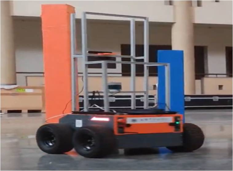
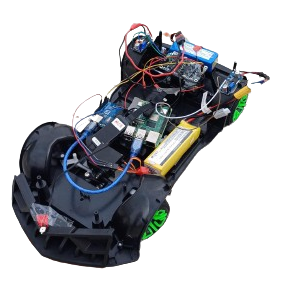
Figure 1: Test setups: Copernicus (left); FOCAS-Car (right).

Intending to address the above challenges, we propose a new class of CBFs via the concept of collision cones. In particular, we generate a new class of constraints that ensure that the relative velocity between the obstacle and the vehicle always points away from the direction of the vehicle’s approach. Assuming ellipsoidal shape for the obstacles [17], the resulting set of unwanted directions for potential collision forms a conical shape, giving rise to the synthesis of Collision Cone Control Barrier Functions (C3BFs). The C3BF-based QP optimally and rapidly calculates inputs in real-time such that the relative velocity vector direction is kept out of the collision cone for all time. This approach is demonstrated using the acceleration-controlled non-holonomic models (Fig. 1).

The idea of collision cones was first introduced in [18, 19, 17] as a means to geometrically represent the possible set of velocity vectors of the vehicle that lead to a collision. The approach was extended for irregularly shaped robots and obstacles with unknown trajectories both in 2D [17] and 3D space [20]. This was commonly used for offline obstacle-free path planning applications [21, 22] like missile guidance. Collision cones have already been incorporated into MPC by defining the cones as constraints [23], but making it a CBF-based constraint has yet to be addressed.

I-A Contribution and Paper Structure

The main contribution of our work is to include the velocity information of the obstacles in the CBFs, thereby yielding a real-time dynamic obstacle avoidance controller. Our specific contributions include the following:

• We formulate a new class of CBFs by using the concept of collision cones. The resulting CBF-QP can be computed in real-time, thereby yielding a safeguarding controller that avoids collision with moving obstacles. This can be stacked over any state-of-the-art planning algorithm with the C3BF-QP acting as a safety filter.

• We formally show how the proposed formulation yields a safeguarding control law for wheeled robots with nonholonomic constraints (i.e. acceleration-controlled unicycle & bicycle models). Note that much of the existing works on CBFs for mobile robots are with point mass models, and our contributions here are for nonholonomic wheeled robots, which are more challenging to control. We demonstrate our solutions in both simulations and hardware experiments.

II Background

In this section, we provide the relevant background necessary to formulate our problem of moving obstacle avoidance. Specifically, we first describe the vehicle models considered in our work, namely the acceleration-controlled unicycle and the bicycle models. Next, we formally introduce Control Barrier Functions (CBFs) and their importance for real-time safety-critical control for considered vehicle models. Finally, we explain the shortcomings in existing CBF approaches in the context of collision avoidance of moving obstacles.

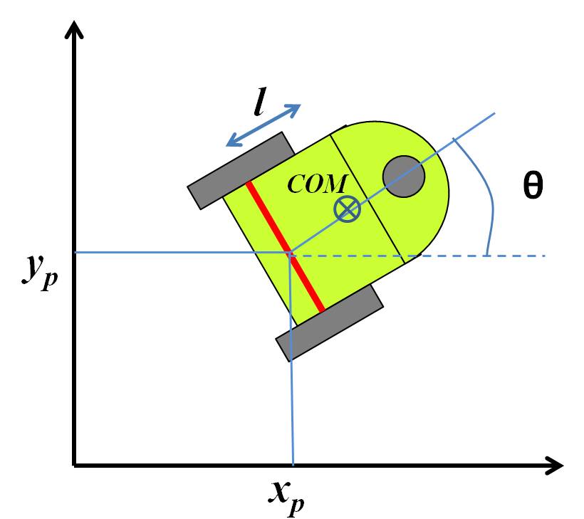
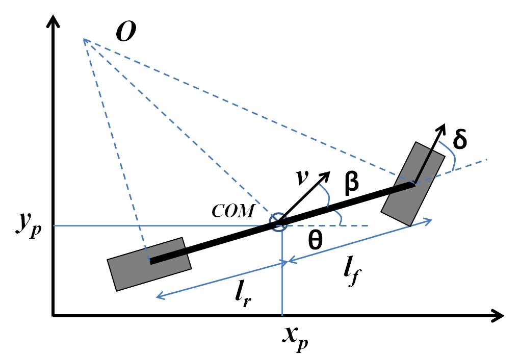
Figure 2: Schematic of Unicycle (left); Bicycle model (right).

II-A Vehicle Models

II-A1 Acceleration controlled unicycle model

The unicycle model encompasses state variables denoted as $x_{p}$, $y_{p}$, $\theta$, $v$, and $\omega$, representing pose, linear velocity, and angular velocity, respectively. Linear acceleration $(a)$ and angular acceleration $(\alpha)$ serve as the control inputs. In Figure 2, a differential drive robot is depicted, which is effectively described by the unicycle model presented below:

$$\begin{bmatrix}\dot{x}_{p}\\ \dot{y}_{p}\\ \dot{\theta}\\ \dot{v}\\ \dot{\omega}\end{bmatrix}=\begin{bmatrix}v\cos\theta\\ v\sin\theta\\ \omega\\ 0\\ 0\end{bmatrix}+\begin{bmatrix}0&0\\ 0&0\\ 0&0\\ 1&0\\ 0&1\end{bmatrix}\begin{bmatrix}a\\ \alpha\end{bmatrix}.$$ (1)

While the conventional unicycle model found in the literature typically employs linear and angular velocities, denoted as $v$ and $\omega$, as inputs, we opt for accelerations as inputs due to the rationale outlined in [24].

II-A2 Acceleration controlled bicycle model

The bicycle model comprises two wheels, with the front wheel dedicated to steering (refer to Fig. 2). This model finds common application in the domain of self-driving cars, where we simplify the treatment of front and rear wheel sets as a unified virtual wheel for each set. The dynamics of the bicycle model are outlined as follows:

$$\begin{bmatrix}\dot{x}_{p}\\ \dot{y}_{p}\\ \dot{\theta}\\ \dot{v}\end{bmatrix} =\begin{bmatrix}v\cos(\theta+\beta)\\ v\sin(\theta+\beta)\\ \frac{v}{l_{r}}\sin(\beta)\\ a\end{bmatrix},$$ (2)

$$\text{where}\quad\beta =\tan^{-1}\left(\frac{l_{r}}{l_{f}+l_{r}}\tan(\delta)\right),$$ (3)

$x_{p}$ and $y_{p}$ denote the coordinates of the vehicle’s center of mass (CoM) in an inertial frame. $\theta$ represents the orientation of the vehicle with respect to the $x$ axis. $a$ is the linear acceleration at CoM. $l_{f}$ and $l_{r}$ are the distances of the front and rear axles from the CoM, respectively. $\delta$ is the steering angle of the vehicle and $\beta$ is the vehicle’s slip angle, i.e., the steering angle of the vehicle mapped to its CoM (see Fig. 2). This is not to be confused with the tire slip angle.

Remark 1

Similar to [8], we assume that the slip angle is constrained to be small. As a result, we approximate $\cos\beta\approx 1$ and $\sin\beta\approx\beta$. Accordingly, we get the following simplified dynamics of the bicycle model:

$$\underbrace{\begin{bmatrix}\dot{x}_{p}\\ \dot{y}_{p}\\ \dot{\theta}\\ \dot{v}\end{bmatrix}}_{\dot{x}}=\underbrace{\begin{bmatrix}v\cos\theta\\ v\sin\theta\\ 0\\ 0\end{bmatrix}}_{f(x)}+\underbrace{\begin{bmatrix}0&-v\sin\theta\\ 0&v\cos\theta\\ 0&\frac{v}{l_{r}}\\ 1&0\end{bmatrix}}_{g(x)}\underbrace{\begin{bmatrix}a\\ \beta\end{bmatrix}}_{u}.$$ (4)

Since the control inputs $a,\beta$ are now affine in the dynamics, CBF-QPs can be constructed directly to yield real-time control laws, as explained next.

II-B Control barrier functions (CBFs)

After providing an overview of the vehicle models, we proceed to formally introduce control barrier functions and their application in ensuring safety within the context of a non-linear control system described by the affine equation:

$$\dot{x}=f(x)+g(x)u.$$ (5)

Here, $x$ belongs to the set $\mathcal{D}\subseteq\mathbb{R}^{n}$ representing the system’s state, and $u$ lies in $\mathbb{U}\subseteq\mathbb{R}^{m}$ representing the system’s input. We assume that the functions $f:\mathbb{R}^{n}\rightarrow\mathbb{R}^{n}$ and $g:\mathbb{R}^{n}\rightarrow\mathbb{R}^{n\times m}$ are locally Lipschitz. Given a Lipschitz continuous control law $u=k(x)$, the resulting closed-loop system $\dot{x}=f_{cl}(x)=f(x)+g(x)k(x)$ leads to a solution $x(t)$, with an initial condition of $x(0)=x_{0}$.

Consider a set $\mathcal{C}$ defined as the super-level set of a continuously differentiable function $h:\mathcal{D}\rightarrow\mathbb{R}$ yielding,

$$\mathcal{C} =\{x\in\mathcal{D}\subset\mathbb{R}^{n}:h(x)\geq 0\}$$ (6)

$$\partial\mathcal{C} =\{x\in\mathcal{D}\subset\mathbb{R}^{n}:h(x)=0\}$$ (7)

$$\text{Int}\left(\mathcal{C}\right) =\{x\in\mathcal{D}\subset\mathbb{R}^{n}:h(x)>0\}.$$ (8)

It is assumed that the interior of $\mathcal{C}$ is non-empty, and $\mathcal{C}$ has no isolated points, i.e., $\text{Int}(\mathcal{C})\neq\emptyset$ and the closure of the interior of $\mathcal{C}$ is equal to $\mathcal{C}$. The system is deemed safe with respect to the control law $u=k(x)$ if for any $x(0)\in\mathcal{C}$, it follows that $x(t)\in\mathcal{C}$ for all $t\geq 0$.

We can ascertain the safety provided by the controller $k(x)$ through the use of control barrier functions (CBFs), as defined below.

Definition 1 (Control barrier function (CBF))

Given the set $\mathcal{C}$ defined by (6)-(8), with $\frac{\partial h}{\partial x}(x)\neq 0\;\forall x\in\partial\mathcal{C}$, the function $h$ is called the control barrier function (CBF) defined on the set $\mathcal{D}$, if there exists an extended class $\mathcal{K}$ function $\kappa$ such that for all $x\in\mathcal{D}$:

$$\sup_{u\in\mathbb{U}}\!\left[\underbrace{\mathcal{L}_{f}h(x)+\mathcal{L}_{g}h(x)u}_{\dot{h}\left(x,u\right)}\!+\kappa\left(h(x)\right)\right]\!\geq\!0$$ (9)

where $\mathcal{L}_{f}h(x):=\frac{\partial h}{\partial x}f(x)$ and $\mathcal{L}_{g}h(x):=\frac{\partial h}{\partial x}g(x)$ are the Lie derivatives.

As per [25] and [26], any Lipschitz continuous control law $k(x)$ that satisfies the inequality $\dot{h}+\kappa(h)\geq 0$ ensures the safety of $\mathcal{C}$ given $x(0)\in\mathcal{C}$, and it leads to asymptotic convergence towards $\mathcal{C}$ if $x(0)$ is outside of $\mathcal{C}$. Notably, CBFs can also be defined solely on $\mathcal{C}$, ensuring only safety. This will find utility in the bicycle model (4), which is elaborated upon later.

II-C Controller synthesis for real-time safety

Having described the CBF and its associated formal results, we now discuss its Quadratic Programming (QP) formulation. CBFs are typically regarded as safety filters which take the desired input (reference controller input) $u_{ref}(x,t)$ and modify this input in a minimal way:

$$u^{*}(x,t) =\min_{u\in\mathbb{U}\subseteq\mathbb{R}^{m}}\left\lVert u-u_{ref}(x,t)\right\rVert^{2}$$ (10)

$$\textrm{s.t. }\mathcal{L}_{f}h(x)+\mathcal{L}_{g}h(x)u+\kappa\left(h(x)\right)\geq 0$$

This is called the Control Barrier Function based Quadratic Program (CBF-QP). The reference control input can be from any SOTA algorithm. If $\mathbb{U}=\mathbb{R}^{m}$, then the QP is feasible, and the explicit solution is given by

$$u^{*}(x,t)=u_{ref}(x,t)+u_{safe}(x,t),$$

where $u_{safe}(x,t)$ is given by

$$u_{safe}(x,t)\!=\!\begin{cases}0&\text{for }\psi(x,t)\geq 0\\ -\frac{\mathcal{L}_{g}h(x)^{T}\psi(x,t)}{\mathcal{L}_{g}h(x)\mathcal{L}_{g}h(x)^{T}}&\text{for }\psi(x,t)<0,\end{cases}$$ (11)

where $\psi(x,t):=\dot{h}\left(x,u_{ref}(x,t)\right)+\kappa\left(h(x)\right)$. The sign change of $\psi$ yields a switching type of control law.

II-D Classical CBFs and moving obstacle avoidance

Having introduced CBFs, we now explore collision avoidance in Unmanned Ground Vehicles (UGVs). In particular, we discuss the problems associated with the classical CBF-QPs, especially with the velocity obstacles. We also summarize and compare with C3BFs in Table I.

TABLE I: Comparison between the Ellipse CBF (12), HOCBF (15) and the proposed C3BF (18) for different UGV models.

CBFs	Vehicle Models	Static Obstacle $(c_{x},c_{y})$	Moving Obstacle $(c_{x}(t),c_{y}(t))^{\dagger}$
Ellipse CBF	Acceleration-controlled unicycle (1)	Not a valid CBF	Not a valid CBF
Ellipse CBF	Bicycle (4)	Valid CBF, No acceleration	Not a valid CBF
HOCBF	Acceleration-controlled unicycle (1)	Valid CBF, No steering	Valid CBF, but conservative
HOCBF	Bicycle (4)	Valid CBF	Not a valid CBF
C3BF	Acceleration-controlled unicycle (1)	Valid CBF in $\mathcal{D}$	Valid CBF in $\mathcal{D}$
C3BF	Bicycle (4)	Valid CBF in $\mathcal{C}$	Valid CBF in $\mathcal{C}$

• $(c_{x}(t),c_{y}(t))$ are continuous (or at least piece-wise continuous) functions of time

II-D1 Ellipse-CBF Candidate - Unicycle

Consider the following CBF candidate:

$$h(x,t)=\left(\frac{c_{x}(t)-x_{p}}{c_{1}}\right)^{2}+\left(\frac{c_{y}(t)-y_{p}}{c_{2}}\right)^{2}-1,$$ (12)

which approximates an obstacle with an ellipse with center $(c_{x}(t),c_{y}(t))$ and axis lengths $c_{1},c_{2}$. We assume that $c_{x}(t),c_{y}(t)$ are differentiable and their derivatives are piece-wise constants. Since $h$ in (12) is dependent on time (e.g., moving obstacles), the resulting set $\mathcal{C}$ is also dependent on time. To analyze this class of sets, time-dependent versions of CBFs can be used [27]. Alternatively, we can reformulate our problem to treat the obstacle position $c_{x},c_{y}$ as states, with their derivatives being constants. This will allow us to continue using the classical CBF given by Definition 1, including its properties on safety. The derivative of (12) is

$$\dot{h}=\frac{2(c_{x}-x_{p})(\dot{c}_{x}-v\cos\theta)}{c_{1}^{2}}+\frac{2(c_{y}-y_{p})(\dot{c}_{y}-v\sin\theta)}{c_{2}^{2}},$$ (13)

which has no dependency on the inputs $a,\alpha$. Hence, $h$ will not be a valid CBF for the acceleration-based model (1).

However, for static obstacles, if we choose to use the velocity-controlled model (with $v,\omega$ as inputs instead of $a,\alpha$), then $h$ will certainly be a valid CBF, but the vehicle will have limited control capability, i.e., it looses steering $\omega$.

II-D2 Ellipse-CBF Candidate - Bicycle

For the bicycle model, the derivative of $h$ (12) yields

$$\dot{h}= 2(c_{x}-x_{p})(\dot{c}_{x}-v\cos\theta+v(\sin\theta)\beta)/c_{1}^{2}$$

$$+2(c_{y}-y_{p})(\dot{c}_{y}-v\sin\theta-v(\cos\theta)\beta)/c_{2}^{2},$$ (14)

which only has $\beta$ as the input. Furthermore, the derivatives $\dot{c}_{x},\dot{c}_{y}$ are free variables, i.e., the obstacle velocities can be selected in such a way that the constraint $\dot{h}(x,u)+\kappa(h(x))<0$, whenever $\mathcal{L}_{g}h=0$. This implies that $h$ is not a valid CBF for moving obstacles for the bicycle model.

II-D3 Higher Order CBFs

It is worth mentioning that for the acceleration-controlled nonholonomic models (1), we can use another class of CBFs introduced specifically for constraints with higher relative degrees: HOCBF [28, 29, 30] given by:

$$h_{2}=\dot{h}_{1}+\kappa(h_{1}),$$ (15)

where $h_{1}$ is the equation of ellipse given by (12).

Apart from lacking geometrical intuition, $h_{2}$ for acceleration-controlled unicycle model will result in a conservative, safe set as per [16, Theorem 3]. For acceleration controlled bicycle model (2) with same HOCBF $h_{2}$ (15), if $\mathcal{L}_{g}h_{2}=0$ then we can choose $\dot{c}_{x},\dot{c}_{y}$ in such a way that $\mathcal{L}_{f}h_{2}+\frac{\partial h_{2}}{\partial t}\ngeq 0$ which results in an invalid CBF. Due to space constraints, a detailed proof of the same is omitted and will be explained as part of future work. The results are summarised in Table-I.

However, our goal in this paper is to develop a CBF formulation with geometrical intuition that provides safety guarantees to avoid moving obstacles with the acceleration-controlled nonholonomic models. We propose this next.

III Collision Cone CBF

After highlighting the limitations of current collision avoidance methods, we will now introduce our proposed approach, which we refer to as Collision Cone Control Barrier Functions (C3BFs).

A collision cone, defined for a pair of objects, represents a predictive set used to assess the potential for a collision between them based on their relative velocity direction. Specifically, it signifies the directions in which either object, if followed, would lead to a collision between the two.

Throughout this paper, we consider obstacles as ellipses, treating the vehicle as a point. Henceforth, when we mention the term ”collision cone”, we are referring to this scenario, with the center of the Unmanned Ground Vehicle (UGV) as the point of reference.

Consider a UGV defined by the system (5) and a moving obstacle (e.g., a pedestrian or another vehicle). This is visually depicted in Figure 3. We establish the velocity and positions of the obstacle relative to the UGV. To account for the UGV’s dimensions, we approximate the obstacle as an ellipse and draw two tangents from the vehicle’s center to a conservative circle that encompasses the ellipse (taking into consideration the UGV’s dimensions as $r=\max(c_{1},c_{2})+\frac{w}{2}$), where $c_{1},c_{2}$ are the dimensions of the ellipse and $w$ is the maximum dimension of the UGV. By over-approximating the obstacle as a circle, we enhance the safety threshold and remove complexity related to the orientation of the obstacle.

For a collision to occur, the relative velocity of the obstacle must be directed towards the UGV. Consequently, the relative velocity vector should not point into the shaded pink region labeled EHI in Figure 3, which takes the form of a cone.

Let $\mathcal{C}$ denote this set of safe directions for the relative velocity vector. If there exists a function $h:\mathcal{D}\subseteq\mathbb{R}^{n}\rightarrow\mathbb{R}$ that satisfies the conditions outlined in Definition 1 on $\mathcal{C}$, then we can assert that a Lipschitz continuous control law derived from the resulting Quadratic Program (QP) (10) for the system ensures that the vehicle will avoid colliding with the obstacle, even if the reference control signal $u_{ref}$ attempts to steer them towards a collision course.

This innovative approach, which avoids the pink cone region, gives rise to what we term as Collision Cone Control Barrier Functions (C3BFs).

Figure 3: Construction of collision cone for an elliptical obstacle considering the UGV’s dimensions (width: $w$).

III-A Application to systems

III-A1 Acceleration controlled unicycle model

We first obtain the relative position vector between the body center of the unicycle and the center of the obstacle. Therefore, we have

$$p_{\rm{rel}}:=\begin{bmatrix}c_{x}-(x_{p}+l\cos\theta)\\ c_{y}-(y_{p}+l\sin\theta)\end{bmatrix}.$$ (16)

Here, $l$ is the distance of the body center from the differential drive axis (see Fig. 2). We obtain its velocity as

$$v_{\rm{rel}}:=\begin{bmatrix}\dot{c}_{x}-(v\cos\theta-l\sin\theta*\omega)\\ \dot{c}_{y}-(v\sin\theta+l\cos\theta*\omega)\end{bmatrix}.$$ (17)

We propose the following CBF candidate:

$$h(x,t)=<p_{\rm{rel}},v_{\rm{rel}}>+\|p_{\rm{rel}}\|\|v_{\rm{rel}}\|\cos\phi,$$ (18)

where $\phi$ is the half angle of the cone, the expression of $\cos\phi$ is given by $\frac{\sqrt{\|p_{\rm{rel}}\|^{2}-r^{2}}}{\|p_{\rm{rel}}\|}$ (see Fig. 3). $<.\>,\>.>$ denotes the inner product of two vectors. The constraint simply ensures that the angle between $p_{\rm{rel}},v_{\rm{rel}}$ is less than $180^{\circ}-\phi$. We have the following first result of the paper:

Theorem 1

Given the acceleration controlled unicycle model (1), the proposed CBF candidate (18) with $p_{\rm{rel}},v_{\rm{rel}}$ defined by (16), (17) is a valid CBF defined for the set $\mathcal{D}$.

Please refer to [24, Thm 1] for the proof of Theorem 1

III-A2 Acceleration controlled Bicycle model

For the approximated bicycle model (4), we define the following:

$$p_{\rm{rel}}:= \begin{bmatrix}c_{x}-x_{p}&c_{y}-y_{p}\end{bmatrix}^{T}$$ (19)

$$v_{\rm{rel}}:= \begin{bmatrix}\dot{c}_{x}-v\cos\theta&\dot{c}_{y}-v\sin\theta\end{bmatrix}^{T}.$$ (20)

Here, $v_{\rm{rel}}$ is NOT equal to the relative velocity $\dot{p}_{\rm{rel}}$. However, for small $\beta$, we can assume that $v_{\rm{rel}}$ is the difference between obstacle velocity and the velocity component along the length of the vehicle $v\cos\beta\approx v$. In other words, the goal is to ensure that this approximated velocity $v_{\rm{rel}}$ is pointing away from the cone. This is an acceptable approximation as $\beta$ is small and the obstacle radius chosen was conservative (see Fig. 3). We have the following result:

Theorem 2

Given the bicycle model (4), the proposed candidate CBF (18) with $p_{\rm{rel}},v_{\rm{rel}}$ defined by (19), (20) is a valid CBF defined for the set $\mathcal{C}$.

Please refer to [24, Thm 2] for the proof of Theorem 2

III-A3 Point mass model

Similar to Theorem 2, we can establish similar results for simple point mass models [14] of the form:

$$\begin{bmatrix}\dot{p}\\ \dot{v}\end{bmatrix}=\begin{bmatrix}0_{2x2}&I_{2x2}\\ 0_{2x2}&0_{2x2}\end{bmatrix}\begin{bmatrix}p\\ v\\ \end{bmatrix}+\begin{bmatrix}0_{2x2}\\ I_{2x2}\end{bmatrix}u,$$ (21)

where $p$ = [$x_{p}$, $y_{p}$]^T, $v$ = [$v_{x}$, $v_{y}$]^T, and $u$ = [$a_{x}$, $a_{y}$]^T $\in\mathbb{R}^{2}$ denotes the position, velocity and acceleration inputs, respectively. The proposed C3BF-QP is indeed a valid CBF, and its proof is straightforward.

IV Results

In this section, we provide the simulation and experimental results to validate the proposed C3BF-QP. We will first demonstrate the results graphically in Python simulations and then on the Copernicus UGV (modeled as a unicycle) and the FOCAS-Car (modeled as a bicycle).

IV-A Acceleration Controlled Unicycle Model

In both simulation and experiments, we have considered the reference control inputs as a simple proportional controller formulated as follows:

$$u_{ref}(x)=\begin{bmatrix}a_{ref}(x)\\ \alpha_{ref}(x)\end{bmatrix}=\begin{bmatrix}k_{1}*(v_{des}-v)\\ -k_{2}*\omega\end{bmatrix},$$ (22)

where $k_{1},k_{2}$ are constant gains, $v_{des}\leq v_{max}$ is the target velocity of vehicle. We chose constant target velocities for verifying the C3BF-QP. For the class $\mathcal{K}$ function in the CBF inequality, we chose $\kappa(h)=\gamma h$, where $\gamma=1$.

Note that the reference controller can be replaced by any existing trajectory tracking / path-planning / obstacle-avoiding controller like the Stanley controller [31] or MPC [32]. Thus, by integrating the C3BF safety filter with existing state-of-the-art algorithms, we can provide formal guarantees on their safety concerning obstacle avoidance.

A virtual perception boundary was incorporated, considering the maximum range for the perception sensors. As soon as an obstacle is detected within the perception boundary, the C3BF-QP is activated with $u_{ref}$ given by (22). The QP yields the optimal accelerations, which are then applied to the robot.

IV-A1 Python Simulations

We consider different scenarios with different poses and velocities of both the vehicle and the obstacle. Different scenarios include static obstacles resulting in a) turning, b) braking and moving obstacles resulting in c) reversing, and d) overtaking, as shown in Fig. 4. The corresponding evolution of CBF value ($h$) as a function of time is shown in Fig. 5. We can observe that even if $h<0$ at t = 0 (Fig. 5(b), (c)), the magnitude is exponentially decreasing and becoming positive.

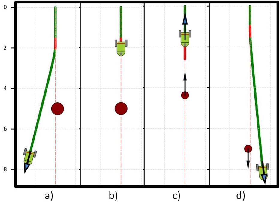
Figure 4: Different acceleration-controlled unicycle model behaviors with static (a,b) & moving (c,d) obstacle. a) turning; b) braking; c) reversing; d) overtaking. The orange lines represent the points where C3BF is active.

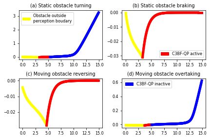
Figure 5: CBF value (h) (Y-axis) varying with time (X-axis). C3BF-QP active means $u_{safe}\neq 0$ (Red) and C3BF-QP inactive means $u_{safe}=0$ (Blue).

IV-A2 Hardware Experiments

Corresponding to the cases tested in Python simulation, experiments were performed on Botsync’s Copernicus UGV (Fig. 1). It is a differential drive (4X4) robot with 860 x 760 x 590 mm dimensions. Apart from its internal wheel encoders, external sensors like Ouster OS1-128 Lidar and Xsens IMU MTI-670G sensor were used for localization and minimizing the odometric error through LIO-SAM algorithm [33]. Zed-2 Stereo camera was used to detect the obstacles through masking and image segmentation techniques and to get their positions using depth information as shown in Fig 6.

Our C3BF algorithm combined with the perception stack was first simulated in the Gazebo environment and then tested on the actual robot. We observed braking, turning, reversal, and overtaking behaviors depending on the initial poses of Copernicus, different positions, and velocities of obstacles. These behaviors were similar to the results obtained from Python simulations. We also experimented with various scenarios with multiple stationary obstacles. Even though the behaviors are sensitive to the initial conditions of the robot and obstacle, collision is avoided in all cases. All the results are shown in the attached video link${}^{\ref{note: Videos link}}$.

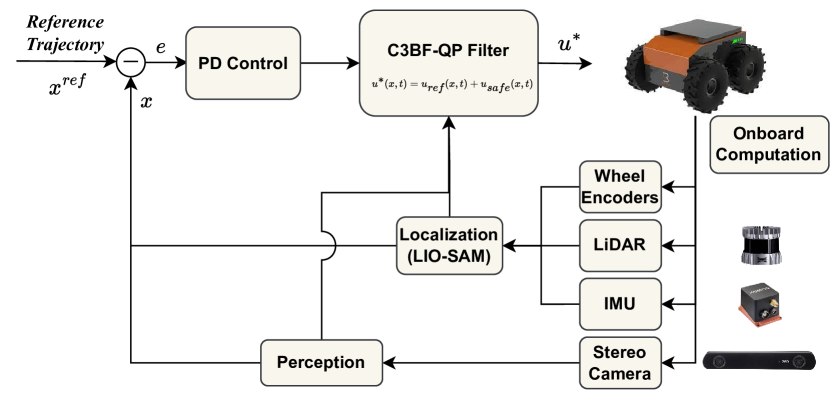
Figure 6: Experimental Setup for Copernicus UGV

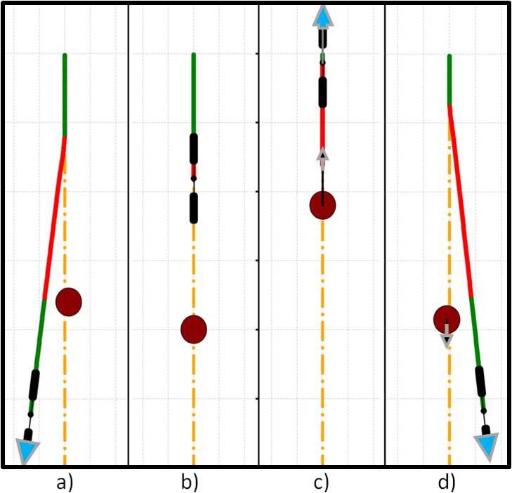
Figure 7: Different acceleration-controlled bicycle model behaviors with static (a,b) & moving (c,d) obstacle. a) turning; b) braking; c) reversing; d) overtaking.

IV-B Acceleration Controlled Bicycle Model

We have extended and validated our C3BF algorithm for the bicycle model (4) which is a good approximation of actual car dynamics in low-speed scenarios where the lateral acceleration is small ($\leq 0.5\mu g$, $\mu$ is the friction co-efficient) [8] [34]. We first simulated all the same four cases without any trajectory tracking reference controller as we did for the unicycle model (Section IV-A1) and got similar results as shown in Fig. 7. For the second set of simulations, the reference acceleration $a_{ref}$ was obtained from a P-controller tracking the desired velocity, while the reference steering $\beta_{ref}$ was obtained from the Stanley controller [31]. The Stanley controller is fed an explicit reference spline trajectory for tracking, with an obstacle on it. The reference controllers were integrated with the C3BF-QP and applied to the robot simulated in Python (Fig. 8) and CARLA simulator.

IV-B1 Python Simulations

Fig. 7 shows different behaviors (turning, braking, reversing, overtaking) of the vehicle modeled as a bicycle model without reference trajectory tracking. Fig. 8 shows the trajectory setup along with an obstacle placed towards the end. The vehicle tracks the reference spline trajectory (red), and the reflection of the collision cone is shown by the pink region. The C3BF algorithm preemptively prevents the relative velocity vector from falling into the unsafe set, thus avoiding obstacles by circumnavigating. It can be verified from Fig. (8(b)) that the slip angle $\beta$ remains small, which is in line with the assumption used (4).

(a) Ego Vehicle avoiding static obstacle (black arrow: $-v_{\rm{rel}}$).

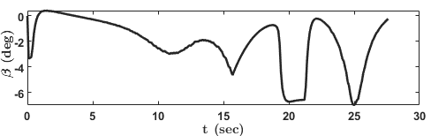
(b) Variation of slip angle ($\beta$) w.r.t. time.

Figure 8: Graphical illustration of C3BF on bicycle model (4).

IV-B2 CARLA Simulations

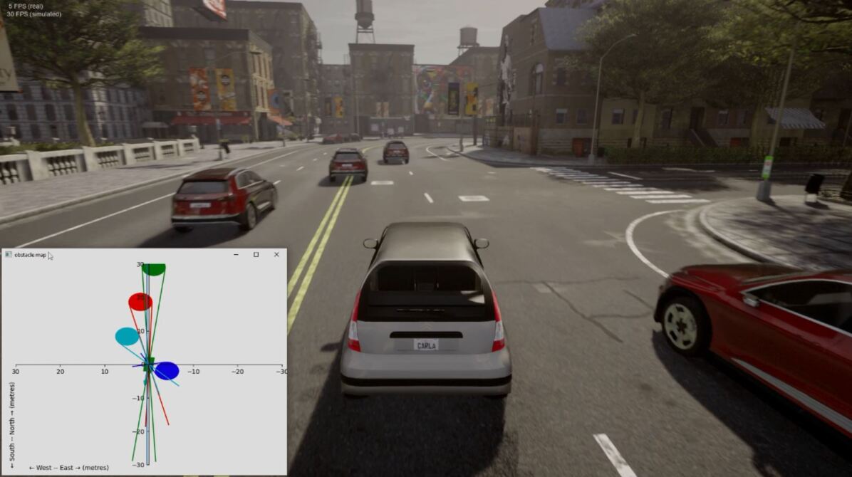
Figure 9: Ego-vehicle (white) avoiding multiple moving cars (Red) using C3BF controller with graphical collision cones.

With the small $\beta$ approximation and using the formulation from Section III-A2, numerical simulations (using CVXOPT library) were performed on virtual car model on CARLA simulator [35] to demonstrate the efficacy of C3BF in collision avoidance in real-world like environments (Fig. 9). A virtual perception boundary was used to accommodate the range of perception sensors on real self-driving cars. Information about the obstacle is programmatically retrieved from the CARLA server. The resulting simulation experiments can be viewed in the attached video link${}^{\ref{note: Videos link}}$.

IV-B3 Hardware Experiments

Corresponding to the cases tested in Python simulation, experiments were performed on FOCAS-Car (Fig. 1), a rear wheel drive car $1/10th$ scaled model, which is powered by 11.1 V, 1800 mAh LIPO Battery. The steering actuation is handled by a servo motor TowerPro MG995, and a DC motor actuates the rear wheels. The realization of the proposed controller has been divided into two stages: a high-level controller running ROS (Robotic Operating System) on Ubuntu and a low-level controller realized by an Arduino UNO board. The sampling rate for the ROS master is set to 100 Hz. The Raspberry Pi 4 board runs Ubuntu 20.04 LTS and ROS Noetic on the processor. It is mounted on the car and solves the optimization problem (C3BF-QP) online. The controller has been coded as a ROS Node in Python. At the low level, this controller has less computation, and it runs at a frequency of 57600 BaudRate. The global position of the car, as well as the obstacle(s), is measured using PhaseSpace^™ motion capture system with a tracking frequency of 960 $Hz$. The 2 LED Markers are placed in front and rear of the car as shown in Fig. 10 to estimate the state of the car ($p,v,\theta,\omega$).

Similar to the experiments conducted in the Python case, we observed braking, turning, and overtaking behaviors. These behaviors were identical to the results obtained from Python simulations. Irrespective of the initial conditions of the robot and the obstacle, collision is avoided in all cases.

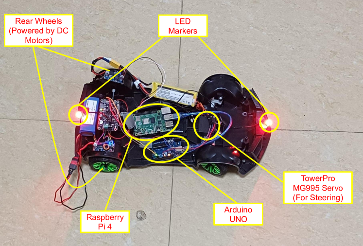
Figure 10: FOCAS-Car Hardware Setup

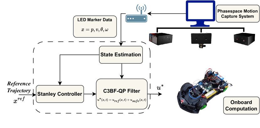
Figure 11: Experimental Setup for FOCAS-Car.

All the simulations and hardware experiments can be viewed in the attached video link

V Conclusions

In this paper, we presented a novel real-time control methodology for Unmanned Ground Vehicles (UGVs) for avoiding moving obstacles by using the concept of collision cones. This idea of constructing a cone around an obstacle is a well-known technique used in planning [18, 19, 17, 20], and this enables the vehicle to check the existence of any collision with moving objects. We have extended the same idea with control barrier functions (CBFs) with acceleration-controlled nonholonomic UGV models (unicycle and bicycle models), thereby enabling fast modification of reference control inputs giving guarantees of collision avoidance in real-time. The proposed QP formulation (C3BF-QP) acts as a filter on the reference controller allowing the vehicle to safely maneuver under different scenarios presented in the paper. Our C3BF safety filter can be integrated with any existing state-of-the-art trajectory tracking/path-planning/obstacle-avoiding algorithms to ensure real-time safety by giving formal guarantees. We validated the proposed C3BF controller in simulations as well as hardware by integrating it with simple trajectory-tracking reference controllers. As a part of future work, the focus will be more on self-driving vehicles with complex dynamic models for avoiding moving obstacles on the road.

References

- [1] S. Yu, M. Hirche, Y. Huang, H. Chen, and F. Allgöwer, “Model predictive control for autonomous ground vehicles: a review,” Autonomous Intelligent Systems, vol. 1, 2021.
- [2] I. Kolmanovsky, E. Garone, and S. Di Cairano, “Reference and command governors: A tutorial on their theory and automotive applications,” in American Control Conference, 2014, pp. 226–241.
- [3] S. Bansal, M. Chen, S. Herbert, and C. J. Tomlin, “Hamilton-jacobi reachability: A brief overview and recent advances,” in 2017 IEEE 56th Annual Conference on Decision and Control (CDC), 2017, pp. 2242–2253.
- [4] Z. Li, “Comparison between safety methods control barrier function vs. reachability analysis,” arXiv preprint arXiv:2106.13176, 2021.
- [5] A. W. Singletary, K. Klingebiel, J. R. Bourne, N. A. Browning, P. T. Tokumaru, and A. D. Ames, “Comparative analysis of control barrier functions and artificial potential fields for obstacle avoidance,” 2021 IEEE/RSJ International Conference on Intelligent Robots and Systems (IROS), pp. 8129–8136, 2021.
- [6] A. Manjunath and Q. Nguyen, “Safe and robust motion planning for dynamic robotics via control barrier functions,” in 60th IEEE Conference on Decision and Control (CDC), 2021, pp. 2122–2128.
- [7] A. D. Ames, J. W. Grizzle, and P. Tabuada, “Control barrier function based quadratic programs with application to adaptive cruise control,” in 53rd IEEE Conference on Decision and Control, 2014, pp. 6271–6278.
- [8] S. He, J. Zeng, B. Zhang, and K. Sreenath, “Rule-based safety-critical control design using control barrier functions with application to autonomous lane change,” in American Control Conference (ACC). IEEE, 2021, pp. 178–185.
- [9] Y. Chen, H. Peng, and J. Grizzle, “Obstacle avoidance for low-speed autonomous vehicles with barrier function,” IEEE Transactions on Control Systems Technology, vol. 26, no. 1, pp. 194–206, 2018.
- [10] T. D. Son and Q. Nguyen, “Safety-critical control for non-affine nonlinear systems with application on autonomous vehicle,” in IEEE 58th Conference on Decision and Control (CDC), 2019, pp. 7623–7628.
- [11] Y. Chen, A. Singletary, and A. D. Ames, “Guaranteed obstacle avoidance for multi-robot operations with limited actuation: A control barrier function approach,” IEEE Control Systems Letters, vol. 5, no. 1, pp. 127–132, 2021.
- [12] M. Abduljabbar, N. Meskin, and C. G. Cassandras, “Control barrier function-based lateral control of autonomous vehicle for roundabout crossing,” in 2021 IEEE International Intelligent Transportation Systems Conference (ITSC), 2021, pp. 859–864.
- [13] W. Xiao, C. G. Cassandras, and C. A. Belta, “Bridging the gap between optimal trajectory planning and safety-critical control with applications to autonomous vehicles,” Automatica, vol. 129, p. 109592, 2021.
- [14] C. Li, Z. Zhang, A. Nesrin, Q. Liu, F. Liu, and M. Buss, “Instantaneous local control barrier function: An online learning approach for collision avoidance,” arXiv preprint arXiv:2106.05341, 2021.
- [15] M. Marley, R. Skjetne, and A. R. Teel, “Synergistic control barrier functions with application to obstacle avoidance for nonholonomic vehicles,” in American Control Conference (ACC), 2021, pp. 243–249.
- [16] W. Xiao and C. Belta, “High-order control barrier functions,” IEEE Transactions on Automatic Control, vol. 67, no. 7, pp. 3655–3662, 2022.
- [17] A. Chakravarthy and D. Ghose, “Obstacle avoidance in a dynamic environment: a collision cone approach,” IEEE Transactions on Systems, Man, and Cybernetics - Part A: Systems and Humans, vol. 28, no. 5, pp. 562–574, 1998.
- [18] P. Fiorini and Z. Shiller, “Motion planning in dynamic environments using the relative velocity paradigm,” in [1993] Proceedings IEEE International Conference on Robotics and Automation, 1993, pp. 560–565 vol.1.
- [19] ——, “Motion planning in dynamic environments using velocity obstacles,” The International Journal of Robotics Research, vol. 17, no. 7, pp. 760–772, 1998.
- [20] A. Chakravarthy and D. Ghose, “Generalization of the collision cone approach for motion safety in 3-d environments,” Autonomous Robots, vol. 32, no. 3, pp. 243–266, 2012.
- [21] D. Bhattacharjee, A. Chakravarthy, and K. Subbarao, “Nonlinear model predictive control and collision-cone-based missile guidance algorithm,” Journal of Guidance, Control, and Dynamics, vol. 44, no. 8, pp. 1481–1497, 2021.
- [22] J. Goss, R. Rajvanshi, and K. Subbarao, Aircraft Conflict Detection and Resolution Using Mixed Geometric And Collision Cone Approaches. AIAA Guidance, Navigation, and Control Conference and Exhibit, 2004, ch. 0, p. 0.
- [23] M. Babu, Y. Oza, A. K. Singh, K. M. Krishna, and S. Medasani, “Model predictive control for autonomous driving based on time scaled collision cone,” in 2018 European Control Conference (ECC). IEEE, 2018, pp. 641–648.
- [24] P. Thontepu, B. G. Goswami, N. Singh, S. PI, S. Sundaram, V. Katewa, S. Kolathaya et al., “Control barrier functions in ugvs for kinematic obstacle avoidance: A collision cone approach,” arXiv preprint arXiv:2209.11524, 2022.
- [25] A. D. Ames, X. Xu, J. W. Grizzle, and P. Tabuada, “Control barrier function based quadratic programs for safety critical systems,” IEEE Transactions on Automatic Control, vol. 62, no. 8, pp. 3861–3876, 2017.
- [26] A. D. Ames, S. Coogan, M. Egerstedt, G. Notomista, K. Sreenath, and P. Tabuada, “Control barrier functions: Theory and applications,” in 18th European Control Conference (ECC), 2019, pp. 3420–3431.
- [27] M. Igarashi, I. Tezuka, and H. Nakamura, “Time-varying control barrier function and its application to environment-adaptive human assist control,” IFAC-PapersOnLine, vol. 52, no. 16, pp. 735–740, 2019, 11th IFAC Symposium on Nonlinear Control Systems.
- [28] Q. Nguyen and K. Sreenath, “Exponential control barrier functions for enforcing high relative-degree safety-critical constraints,” in American Control Conference (ACC), 2016, pp. 322–328.
- [29] W. Xiao and C. Belta, “Control barrier functions for systems with high relative degree,” in IEEE 58th Conference on Decision and Control (CDC), 2019, pp. 474–479.
- [30] X. Tan, W. S. Cortez, and D. V. Dimarogonas, “High-order barrier functions: Robustness, safety, and performance-critical control,” IEEE Transactions on Automatic Control, vol. 67, no. 6, pp. 3021–3028, 2022.
- [31] G. M. Hoffmann, C. J. Tomlin, M. Montemerlo, and S. Thrun, “Autonomous automobile trajectory tracking for off-road driving: Controller design, experimental validation and racing,” in American Control Conference, 2007, pp. 2296–2301.
- [32] J. Zeng, B. Zhang, and K. Sreenath, “Safety-critical model predictive control with discrete-time control barrier function,” in 2021 American Control Conference (ACC), 2021, pp. 3882–3889.
- [33] T. Shan, B. Englot, D. Meyers, W. Wang, C. Ratti, and R. Daniela, “Lio-sam: Tightly-coupled lidar inertial odometry via smoothing and mapping,” in IEEE/RSJ International Conference on Intelligent Robots and Systems (IROS). IEEE, 2020, pp. 5135–5142.
- [34] P. Polack, F. Altché, B. d’Andréa Novel, and A. de La Fortelle, “The kinematic bicycle model: A consistent model for planning feasible trajectories for autonomous vehicles?” in 2017 IEEE Intelligent Vehicles Symposium (IV), 2017, pp. 812–818.
- [35] A. Dosovitskiy, G. Ros, F. Codevilla, A. Lopez, and V. Koltun, “CARLA: An open urban driving simulator,” in Proceedings of the 1st Annual Conference on Robot Learning, 2017, pp. 1–16.