IFT-UAM/CSIC-22-113

Quantum tomography of helicity states
for general scattering processes.

Alexander Bernal

Instituto de Física Teórica, IFT-UAM/CSIC,
Universidad Autónoma de Madrid, Cantoblanco, 28049 Madrid, Spain

Abstract

Quantum tomography has become an indispensable tool in order to compute the density matrix $\rho$ of quantum systems in Physics. Recently, it has further gained importance as a basic step to test entanglement and violation of Bell inequalities in High-Energy Particle Physics. In this work, we present the theoretical framework for reconstructing the helicity quantum initial state of a general scattering process. In particular, we perform an expansion of $\rho$ over the irreducible tensor operators $\{T^{L}_{M}\}$ and compute the corresponding coefficients uniquely by averaging, under properly chosen Wigner D-matrices weights, the angular distribution data of the final particles. Besides, we provide the explicit angular dependence of both the normalised differential cross section and the generalised production matrix $\Gamma$. Finally, we re-derive all our previous results from a quantum-information perspective using the Weyl-Wigner-Moyal formalism and we obtain in addition simple analytical expressions for the Wigner $P$ and $Q$ symbols.

1 Introduction

The general description of a quantum mechanical system is encoded in a central mathematical entity known as density matrix, $\rho$. In this way, any physical accessible information of the system (any information attained by performing measurements over it) is theoretically obtained by computing expectation values of observables: $\langle{\cal O}\rangle=\Tr{{\cal O}\rho}$. Here, $\cal O$ stands for the Hermitian and linear operator associated with the considered experimental measurement. In particular, when dealing with systems with finite degrees of freedom, i.e. the associated Hilbert space has finite dimension, this quantum characterisation takes the form of a complex, unit-trace and Hermitian matrix. Therefore, in order to test with high precision either new or well-established models of Particle Physics, a practical and accurate reconstruction of $\rho$ is needed.

The procedure to determine this density matrix by performing measurements over the system is known in the quantum-information context as “Quantum Tomography” [1, 2, 3]. Special relevance has been given to the helicity density matrix since the works of E. Wigner[4], M. Jacob [5], G. C. Wick [6] and J. Werle [7, 8, 9] indicated a strong relation between angular distribution of final states and helicity amplitudes for general scattering processes. For instance, different methods for the tomography of single-particle systems [10, 11, 12] and of pairs of particles [13, 14, 15, 16, 17] have been proposed, all of them based on the reconstruction via the angular distribution data of the final particles. Nevertheless, they restrict themselves to final states reached after a chain of consecutive decays, while the plethora of other cases are not addressed. In this study we carry out the extension of the quantum tomography for all possible scattering processes. As a matter of fact, due to the transformation property under rotations of the irreducible tensor operators $\{T^{L}_{M}\}$[18, 11, 12, 17] we base the reconstruction of $\rho$ on its expansion over this suitable basis, contrary to other approaches where either Cartesian vector and tensors [10, 19, 15] or generalised Gell-Mann matrices [20, 16] are used.

As aforementioned, once the density matrix is reconstructed several properties of the corresponding system can be tested. Namely, several theoretical papers have tackled the entanglement in pairs of top and anti-top [14, 21, 22, 23, 24, 25], $\Lambda$ baryons [26], vector bosons [23, 27, 28, 29], top-quarks[22, 30, 31, 32], tau-leptons [31, 33] and photons [31] as well as the violation of Bell inequalities in electron-positron collisions [34], charmonium decays[35, 36], positronium decays [37], Higgs boson decays to $WW$ and $ZZ$ pairs [27, 38, 23, 39, 29], $B^{0}\bar{B}^{0}$ pairs [40], top-quarks [22, 25], tau-leptons [31] and 2-2 scatterings [41, 42]. On the experimental side, works concerning spin-correlations of top anti-top pairs [43, 44] as well as violation of Bell inequalities in ions [45], vector bosons [46], superconducting systems [47], nitrogen vacancies[48] and in photons [49, 50, 51] can also be found in the literature.

To sum up, the situation we will be referring along the work is a scattering process from $m$ initial particles to $n\geq 2$ final particles. Actually, we are interested in the helicity density matrix of the initial state and the only information we have access to is the angular distribution of the final particles. From this starting point, we are able not only to perform the tomography of $\rho$ but also to give the explicit angular dependence of both the generalised production matrix $\Gamma$, see section 3 for a rigorous definition, and of the normalised differential cross section of the process, the latter having been previously studied in [52, 53, 54, 55, 56, 57, 58].

The paper is organised as follows: in section 2 we present the quantum-mechanical formalism for the representation of many-particle systems used throughout the paper. Section 3 is devoted to the construction of the generalised production matrix, while in section 4 we develop the quantum tomography of the density matrix $\rho$ from its relation with both the normalised differential cross section and the generalised production matrix, elaborating on the case in which $\Gamma$ factorises. In section 5 we further compare the theoretical framework here introduced to the Weyl-Wigner-Moyal one [59, 16]. Finally, in section 6 we summarise the whole work and we present our conclusions. Appendix A collects the explicit form of the generalised production matrix for relevant scattering processes in High-Energy Particle Physics, whereas Appendix B is dedicated to mathematical technicalities omitted in the main text.

2 State representation for relativistic many-particle systems

This section is devoted to summarise and recall the formalism of state representations for relativistic many-particle systems [7, 8, 9]. We emphasise on the indispensable concepts for the work.

Let us consider an arbitrary system of $n$ particles with definite $3$-momenta $\vec{p}_{i}$, spins $s_{i}$ and helicities $\lambda_{i}\in\{-s_{i},\dots,s_{i}\}$, such that the total linear momentum $\vec{\chi}=\sum_{i=1}^{n}\vec{p_{i}}=\vec{0}$. In particular, we will denote this centre-of-mass spatial reference frame by $\mathcal{RF}$ and consider $\vec{p}_{i}=p_{i}\,\hat{p}_{i}$, with $p_{i}$ and $\hat{p}_{i}$ the $3$-momentum modulus and unit vector of particle $i$.

Based on these $3$-momenta, we can fix a particularly useful centre-of-mass reference frame as displayed in Fig.1, which we denote by $\mathcal{RF}^{\,0}$. Namely, we set the $3$-momentum of one of the particles (from now on particle $1$) to define the $z$ axis via $\hat{z}=\hat{p}_{1}$, while the $3$-momentum of a second particle (from now on particle $2$) is considered to lie in the $x>0$ half of the $xz$ plane, so that $\hat{y}=\frac{\hat{p}_{1}\crossproduct\hat{p}_{2}}{|\hat{p}_{1}\crossproduct\hat{p}_{2}|}$. Therefore, $\mathcal{RF}^{\,0}$ is completely characterised by the $3$-momentum of the two selected particles, which we have assumed to be distinguishable from the rest and between them.

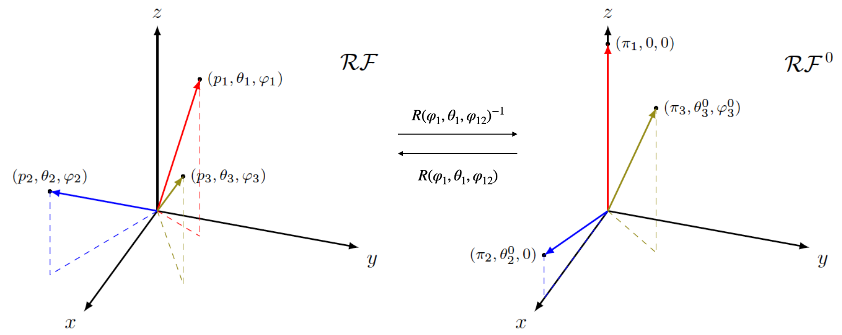
Figure 1: On the left, a sketch of the most general centre-of-mass spatial reference frame of $n$ particles $\mathcal{RF}$ (only three of the $n$ particles are displayed for clarity). On the right, a sketch of the special centre-of-mass reference frame of $n$ particles $\mathcal{RF}^{\,0}$ fixed by particles 1 and 2 (only three of the $n$ particles are displayed). The corresponding Euler rotation to move from one frame to another is also shown.

Moreover, to simplify in what comes the distinction between the $3$-momenta of the particles described with respect to a general frame $\mathcal{RF}$ and with respect to the special one $\mathcal{RF}^{\,0}$, we denote by $\vec{\pi}_{i}$ the $3$-momentum of each particle in the latter. For instance, the spherical coordinates (modulus as well as polar and azimuthal angles) of each $3$-momentum $\vec{\pi}_{i}$ take the values

$$\left(\pi_{1},\theta_{1}^{\,0},\varphi_{1}^{\,0}\right)=\left(\pi_{1},0,0\right),\quad\left(\pi_{2},\theta_{2}^{\,0},\varphi_{2}^{\,0}\right)=\left(\pi_{2},\theta_{2}^{\,0},0\right),\quad\left(\pi_{i},\theta_{i}^{\,0},\varphi_{i}^{\,0}\right)\hbox{ for }i=3,\dots,n.$$ (1)

We notice that only $3n-3$ non-trivial coordinates are needed to describe the system in this frame. On the other hand, the corresponding $3n$ coordinates of $\vec{p}_{i}$ in a general $\mathcal{RF}$ are obtained from the ones in $\mathcal{RF}^{\,0}$ by performing an Euler rotation $R\left(\alpha,\beta,\gamma\right)$ of the whole system as a rigid body.

The inverse operation can also be done: the $\mathcal{RF}^{\,0}$ description is recovered by applying a $R\left(\alpha,\beta,\gamma\right)^{-1}$ rotation to the system described in $\mathcal{RF}$, see Fig.1. In this sense, the physical meaning of the Euler angles characterising the rotation is easily obtained once particles $1$ and $2$ are identified in $\mathcal{RF}$. Specifically, $\left(\alpha,\beta\right)=\left(\varphi_{1},\theta_{1}\right)$ are the angular components of particle $1$ in $\mathcal{RF}$ whereas $\gamma=\varphi_{12}$ is the azimuthal coordinate of particle $2$ after applying an initial $R(\alpha,\beta,0)^{-1}$ rotation to the system, i.e. after setting the $3$-momentum of particle $1$ to be in the $z$ axis.

Following this convention, the quantum state of a general $n$-particle system with definite $3$-momenta and helicities as well as null total linear momentum is given by

$$\prod_{i=1}^{n}\ket{\vec{p}_{i}\,\lambda_{i}}=\hat{D}\left(R\right)\prod_{i=1}^{n}\ket{\vec{\pi}_{i}\,\lambda_{i}}=\ket{R\,\pi\,\lambda},$$ (2)

here $\hat{D}\left(R\right)$ is the unitary representation of the rotation acting on the quantum states $R=R\left(\alpha,\beta,\gamma\right)$ (for simplicity we omit the angle dependence of $R$) and $\vec{p}_{i}=R\,\vec{\pi}_{i}$. In addition, we have denoted by $\lambda$ the whole set of particle’s helicities and by $\pi$ the set of $3n-3$ spherical coordinates needed to describe the system in $\mathcal{RF}^{\,0}$, as specified in Eq.(1). The orthogonality conditions for these states read

$$\bra{R^{\prime}\,\pi^{\prime}\,\lambda^{\prime}}\ket{R\,\pi\,\lambda}=\delta\left(R^{\prime},R\right)\delta\left(\pi\,\pi^{\prime};\lambda\lambda^{\prime}\right),\hbox{ with }\delta\left(R^{\prime},R\right)=\delta\left(\alpha-\alpha^{\prime}\right)\delta\left(\cos{\beta}-\cos{\beta}^{\prime}\right)\delta\left(\gamma-\gamma^{\prime}\right)$$ (3)

$$\displaystyle{\hbox{ and }\delta\left(\pi\,\pi^{\prime};\lambda\lambda^{\prime}\right)=\frac{\delta\left(\pi_{1}-\pi_{1}^{\prime}\right)}{\pi_{1}^{2}}\,\frac{\delta\left(\pi_{2}-\pi_{2}^{\prime}\right)}{\pi_{2}^{2}}\,\frac{\delta\left(\theta_{2}^{\,0}-\theta_{2}^{\,0\,^{\prime}}\right)}{\sin{\theta_{2}^{\,0}}}\,\prod_{i=3}^{n}\delta_{3}\left(\vec{\pi}_{i}-\vec{\pi}_{i}^{\prime}\right)\,\prod_{j=1}^{n}\delta_{\lambda_{j}\,\lambda_{j}^{\prime}}.}$$

Following [9], a more convenient representation of (2) is possible. Namely, the $\pi$ set of quantum numbers is replaced by the total energy of the system $E$, the total linear momentum $\vec{\chi}=\vec{0}$ and a set $\kappa$ of $3n-7$ parameters, functions of $\pi$, to be chosen depending on the case of interest. Whenever $3n-7\leq 0$, we take $\kappa=\varnothing$. Hence, state (2) becomes

$$\displaystyle{\ket{R\,E\,\vec{\chi}\,\kappa\,\lambda},\hbox{ with orthogonality conditions }}$$ (4)

$$\displaystyle{\bra{R^{\prime}\,E^{\prime}\,\vec{\chi}^{\prime}\,\kappa^{\prime}\,\lambda^{\prime}}\ket{R\,E\,\vec{\chi}\,\kappa\,\lambda}=\delta\left(R^{\prime},R\right)\delta\left(E^{\prime}-E\right)\delta_{3}\left(\vec{\chi}^{\prime}-\vec{\chi}\right)\delta\left(\kappa\,\kappa^{\prime};\lambda\lambda^{\prime}\right)}$$

$$\displaystyle{\hbox{ and }\delta\left(\kappa\,\kappa^{\prime};\lambda\lambda^{\prime}\right)=\prod_{i=1}^{3n-7}\delta\left(\kappa_{i}-\kappa_{i}^{\prime}\right)\,\prod_{j=1}^{n}\delta_{\lambda_{j}\,\lambda_{j}^{\prime}}.}$$

Since both $E$ and $\vec{\chi}$ play no role in what follows, the above state representation will be denoted by $\ket{R\,\kappa\,\lambda}$. Finally, let us also introduce the relation between the states in Eq.(4) and those of definite angular momentum:

$$\ket{J\,M\,\Lambda\,\kappa\,\lambda}=\frac{\left(J+1/2\right)^{1/2}}{2\pi}\int dR\,D^{J}_{M\,\Lambda}\left(R\right)^{*}\ket{R\,\kappa\,\lambda},\hbox{ with }$$ (5)

$$\bra{R\,\kappa^{\prime}\,\lambda^{\prime}}\ket{J\,M\,\Lambda\,\kappa\,\lambda}=\frac{\left(J+1/2\right)^{1/2}}{2\pi}D^{J}_{M\,\Lambda}\left(R\right)^{*}\,\delta\left(\kappa\,\kappa^{\prime};\lambda\lambda^{\prime}\right).$$

The function $D^{J}_{M\,M^{\prime}}\left(R\right)\delta_{J\,J^{\prime}}=\bra{J\,M}\hat{D}\left(R\right)\ket{J^{\prime}\,M^{\prime}}$ is the Wigner D-matrix associated with the Euler rotation $R$, $dR$ is the differential with respect to the angles characterising $R$ and the quantum number $\Lambda$ corresponds to the projection of the total angular momentum of the system over $\hat{p}_{1}$. From the orthogonality conditions of the Wigner D-matrices

$$\int dR\,D^{J^{\prime}}_{M^{\prime}\,\Lambda^{\prime}}\left(R\right)^{*}\,D^{J}_{M\,\Lambda}\left(R\right)=\frac{8\pi^{2}}{2J+1}\ \delta_{J\,J^{\prime}}\ \delta_{M\,M^{\prime}}\ \delta_{\Lambda\,\Lambda^{\prime}},$$ (6)

we get

$$\bra{J^{\prime}\,M^{\prime}\,\Lambda^{\prime}\,\kappa^{\prime}\,\lambda^{\prime}}\ket{J\,M\,\Lambda\,\kappa\,\lambda}=\delta_{J\,J^{\prime}}\delta_{M\,M^{\prime}}\delta_{\Lambda\,\Lambda^{\prime}}\delta\left(\kappa\,\kappa^{\prime};\lambda\lambda^{\prime}\right).$$ (7)

Certain properties of these states concerning the transformation under parity $P$ and time inversion $T$, as well as rotations $R$ are

$$\displaystyle{P\ket{J\,M\,\Lambda\,\kappa\,\lambda}=\eta^{\prime}\ket{J\,M\,\left(-\Lambda\right)\,\tilde{\kappa}\,\left(-\lambda\right)},\quad T\ket{J\,M\,\Lambda\,\kappa\,\lambda}=\left(-1\right)^{J-M}\ket{J\,\left(-M\right)\,\Lambda\,\tilde{\kappa}\,\lambda},}$$ (8)

$$\displaystyle{R\ket{J\,M\,\Lambda\,\kappa\,\lambda}=\sum_{M^{\prime}=-J}^{J}D^{J}_{M^{\prime}\,M}(R)\ket{J\,M^{\prime}\,\Lambda\,\kappa\,\lambda},\hbox{ with }\tilde{\kappa}=\kappa\left(\varphi^{\,0}_{i}\to-\varphi^{\,0}_{i}\right),\quad\eta^{\prime}=\left(-1\right)^{J-\Lambda}\prod_{i=1}^{n}\eta_{i}\left(-1\right)^{s_{i}-\lambda_{i}},}$$

where $\eta_{i}$ and $s_{i}$ are, respectively, the intrinsic parity and spin of particle $i$. The inverse relation concerning the states in Eq.(5) is

$$\ket{R\,\kappa\,\lambda}=\sum_{J}\sum_{M\,\Lambda}\frac{(J+1/2)^{1/2}}{2\pi}D^{J}_{M\,\Lambda}(R)\ket{J\,M\,\Lambda\,\kappa\,\lambda}.$$ (9)

A further final comment is needed: during this section we have assumed the particles we are dealing with have a fixed and known mass $m_{i}$. Nevertheless this may not be the case, for example when working with off-shell particles. For those scenarios, we also need to treat $m_{i}$ as an extra quantum number per particle (to add in the parameter set $\kappa$) in order to have a complete representation of the system. Specific examples are analysed in Appendix A.

3 Generalised production matrix

We define the generalised production matrix, sometimes known in the literature as a decay matrix [60, 10], by

$$\Gamma_{\bar{\lambda}\,\bar{\lambda}^{\prime}}\propto\sum_{\lambda}{\cal M}_{\lambda\,\bar{\lambda}}{\cal M}_{\lambda\,\bar{\lambda}^{\prime}}^{*}.$$ (10)

Here, as done in [7, 8, 9], we have denoted the initial state magnitudes with an overbar and the final state ones without it. The amplitudes ${\cal M}_{\lambda\,\bar{\lambda}}$ are the so-called helicity amplitudes, whose expression in term of the scattering matrix $S$ and the states introduced in the previous section is

$${\cal M}_{\lambda\,\bar{\lambda}}=\bra{R\,\kappa\,\lambda}S\ket{\bar{R}\,\bar{\kappa}\,\bar{\lambda}},\quad\hbox{ with }\quad\ket{R\,\kappa\,\lambda}\propto\sum_{J}\sum_{M\,\Lambda}(2J+1)^{1/2}D^{J}_{M\,\Lambda}(R)\ket{JM\Lambda\kappa\lambda}$$ (11)

and similarly with the overbarred magnitudes. The rotations $\bar{R},\,R$ are performed with respect to a fixed reference frame, $\mathcal{RF}^{\,0}$, and along with $\left(\bar{\kappa},\bar{\lambda}\right)$ as well as $\left(\kappa,\lambda\right)$ completely characterise the initial and final states. Furthermore, by definition of (2) and (4), the property

$$\ket{R\,\kappa\,\lambda}=\hat{D}\left(R\right)\ket{\mathbb{1}\,\kappa\,\lambda}$$ (12)

holds, where the notation $\mathbb{1}$ refers to the absence of a rotation and $\hat{D}\left(R\right)$ is the unitary representation of the rotation $R$ in the Hilbert space of interest.

As will be justified later on, see Eq.(37) in section 4 and (59) in section 5, the relevant matrix for our final goal is the transposed of the generalised production matrix, $\Gamma^{T}$. Therefore, plugging the expression of ${\cal M}_{\lambda\,\bar{\lambda}}$ in it:

$$\Gamma^{T}_{\bar{\lambda}\,\bar{\lambda}^{\prime}} \propto \sum_{\lambda}\bra{\bar{R}\,\bar{\kappa}\,\bar{\lambda}}S^{\dagger}\ket{R\,\kappa\,\lambda}\bra{R\,\kappa\,\lambda}S\ket{\bar{R}\,\bar{\kappa}\,\bar{\lambda}^{\prime}}$$

$$= \bra{\bar{R}\,\bar{\kappa}\,\bar{\lambda}}\left[\sum_{\lambda}\left(S^{\dagger}\ket{R\,\kappa\,\lambda}\bra{R\,\kappa\,\lambda}S\right)\right]\ket{\bar{R}\,\bar{\kappa}\,\bar{\lambda}^{\prime}}.$$

Using property (12) of $\ket{R\,\kappa\,\lambda}$ as well as the rotation invariance of the scattering matrix $S$, we get

$$\Gamma^{T}_{\bar{\lambda}\,\bar{\lambda}^{\prime}} \propto \bra{\bar{R}\,\bar{\kappa}\,\bar{\lambda}}\hat{D}\left(R\right)\left[\sum_{\lambda}\left(S^{\dagger}\ket{\mathbb{1}\,\kappa\,\lambda}\bra{\mathbb{1}\,\kappa\,\lambda}S\right)\right]\hat{D}\left(R\right)^{-1}\ket{\bar{R}\,\bar{\kappa}\,\bar{\lambda}^{\prime}}$$

$$= \bra{\bar{\mathbb{1}}\,\bar{\kappa}\,\bar{\lambda}}\left(\hat{D}\left(\bar{R}\right)^{-1}\hat{D}\left(R\right)\right)\left[\sum_{\lambda}\left(S^{\dagger}\ket{\mathbb{1}\,\kappa\,\lambda}\bra{\mathbb{1}\,\kappa\,\lambda}S\right)\right]\left(\hat{D}\left(\bar{R}\right)^{-1}\hat{D}\left(R\right)\right)^{-1}\ket{\bar{\mathbb{1}}\,\bar{\kappa}\,\bar{\lambda}^{\prime}}$$

$$= \bra{\bar{\mathbb{1}}\,\bar{\kappa}\,\bar{\lambda}}\hat{D}\left(\bar{R}^{-1}R\right)\left[\sum_{\lambda}\left(S^{\dagger}\ket{\mathbb{1}\,\kappa\,\lambda}\bra{\mathbb{1}\,\kappa\,\lambda}S\right)\right]\hat{D}\left(\bar{R}^{-1}R\right)^{-1}\ket{\bar{\mathbb{1}}\,\bar{\kappa}\,\bar{\lambda}^{\prime}}.$$

This last equation implies that in the helicity basis for the initial states, $\{\ket{\bar{\mathbb{1}}\,\bar{\kappa}\,\bar{\lambda}}\}_{\bar{\lambda}}$, the matrix $\Gamma^{T}$ only depends on the relative rotation between the initial and final states, i.e. $\Gamma^{T}\left(\bar{R},R\right)=\Gamma^{T}\left(\bar{R}^{-1}R\right)$, and it is given by rotating $\Gamma^{T}\left(\bar{\mathbb{1}},\mathbb{1}\right)=\Gamma^{T}\left(\mathbb{1}\right)$ accordingly, as it should happen for a generic quantum-mechanical operator in a rotated system [18]:

$$\Gamma^{T}\left(\bar{R},R\right)=\Gamma^{T}\left(\bar{R}^{-1}R\right)=\hat{D}\left(\bar{R}^{-1}R\right)\Gamma^{T}(\mathbb{1})\hat{D}\left(\bar{R}^{-1}R\right)^{-1}.$$ (15)

Furthermore, it is worth mentioning that instead of considering two different rotations $\left(\bar{R},\,R\right)$ with respect to the fixed reference frame $\mathcal{RF}^{\,0}$, we can always set the initial state of the scattering process to define $\mathcal{RF}^{\,0}$. Thus, $\bar{R}=\bar{\mathbb{1}}$ and the whole relative rotation only comes from a rotation of the final state with respect to this reference frame, $\bar{R}^{-1}R=R$. Following the physical interpretation given in section 2, the set of Euler angles characterising $R$ are denoted by $\left(\alpha,\beta,\gamma\right)=\left(\varphi_{1},\theta_{1},\varphi_{12}\right)=\Omega$. In consequence,

$$\bar{R}^{-1}R=R=R\left(\varphi_{1},\theta_{1},\varphi_{12}\right)=R\left(\Omega\right)\implies\Gamma^{T}\left(\bar{R}^{-1}R\right)=\Gamma^{T}\left(R\right)=\hat{D}\left(R\right)\Gamma^{T}(\mathbb{1})\hat{D}\left(R\right)^{-1}.$$ (16)

From now on, we consider $\Gamma^{T}\equiv\Gamma^{T}\left(\mathbb{1}\right)$ and specify the argument $\left(\mathbb{1}\right)$ only when needed.

The exact expression for $\Gamma^{T}$ is presented in full detail in Appendix A. For instance, some relevant features of this matrix are discussed for the following scattering processes (labelled in terms of the initial and final particle’s number)

$$1)\ \bar{1}\to 2\quad\quad 2)\ \bar{1}\to n\quad\quad 3)\ \bar{2}\to 2\quad\quad 4)\ \bar{2}\to n\quad\quad 5)\ \bar{m}\to 2\quad\quad 6)\ \bar{m}\to n.$$

In general, the generalised production matrix can be expanded in the canonical basis via a sum over the possible spin projections $\sigma_{i}\in\{-s_{i},\dots,s_{i}\}$ of the initial particles:

$$\displaystyle{\Gamma^{T}\propto\sum_{\sigma\,\sigma^{\prime}}a_{\sigma\,\sigma^{\prime}}\,e_{\sigma\,\sigma^{\prime}},\hbox{ with }\sigma=\left(\sigma_{1},\dots,\sigma_{m}\right)}\hbox{ and same with primas,}$$ (17)

$$\displaystyle{a_{\sigma\,\sigma^{\prime}}=\sum_{\lambda}\bra{\bar{\mathbb{1}}\,\bar{\kappa}\,\sigma}S^{\dagger}\ket{\mathbb{1}\,\kappa\,\lambda}\bra{\mathbb{1}\,\kappa\,\lambda}S\ket{\bar{\mathbb{1}}\,\bar{\kappa}\,\sigma^{\prime}},\quad e_{\sigma\,\sigma^{\prime}}=\bigotimes_{i=1}^{m}e_{\sigma_{i}\,\sigma_{i}^{\prime}},\quad[e_{\sigma_{i}\,\sigma^{\prime}_{i}}]_{\bar{\lambda}_{i},\bar{\lambda}_{i}^{\prime}}=\delta_{\sigma_{i},\bar{\lambda}_{i}}\ \delta_{\sigma_{i}^{\prime},\bar{\lambda}_{i}^{\prime}}.}$$

I.e., $e_{\sigma_{i}\,\sigma_{i}^{\prime}}$ is a matrix unit with the $\left(\sigma_{i},\sigma_{i}^{\prime}\right)$-element equal to $1$ and all the others null. In addition, $a_{\sigma\,\sigma^{\prime}}=a_{\sigma\,\sigma^{\prime}}\left(\bar{\kappa},\kappa\right)$ are a generalisation of the so-called reduced helicity amplitudes [60, 10, 15] and encode the kinematics not included in $\Omega$. Nonetheless, during the current and next sections the $\left(\bar{\kappa},\kappa\right)$ dependence will be in general omitted as it is not relevant for the work.

Moreover, imposing $\Tr{\Gamma^{T}}=\Tr{\Gamma}=1$ we can deduce the normalisation factor as a function of $a_{\sigma\,\sigma^{\prime}}$:

$$\Tr{e_{\sigma\,\sigma^{\prime}}}=\delta_{\sigma\,\sigma^{\prime}}\Longrightarrow\Tr{\sum_{\sigma\,\sigma^{\prime}}a_{\sigma\,\sigma^{\prime}}e_{\sigma\,\sigma^{\prime}}}=\sum_{\sigma}a_{\sigma\,\sigma},\hbox{ where }a_{\sigma\,\sigma}=\sum_{\lambda}\left|\bra{\mathbb{1}\,\kappa\,\lambda}S\ket{\bar{\mathbb{1}}\,\bar{\kappa}\,\sigma}\right|^{2}\in\mathbb{R}^{+}.$$ (18)

Hence, defining $a_{+}\equiv\sum_{\sigma}a_{\sigma\,\sigma}\in\mathbb{R}^{+}$,

$$\Gamma^{T}=\frac{1}{a_{+}}\sum_{\sigma\,\sigma^{\prime}}a_{\sigma\,\sigma^{\prime}}e_{\sigma\,\sigma^{\prime}}\Longrightarrow\Gamma^{T}\left(R\right)=\frac{1}{a_{+}}\sum_{\sigma\,\sigma^{\prime}}a_{\sigma\,\sigma^{\prime}}\hat{D}\left(R\right)e_{\sigma\,\sigma^{\prime}}\hat{D}\left(R\right)^{-1}.$$ (19)

4 Reconstruction of the density matrix

The main goal of this section is to develop the quantum tomography for the initial state helicity density matrix $\rho$. For that purpose, we make use of the relation between the normalised differential cross section, the density matrix and the production matrix [60, 10, 15]:

$$\dfrac{1}{\sigma}\dfrac{d\sigma}{d\Omega\,d\bar{\kappa}\,d\kappa}={\cal N}\Tr{\rho\,\Gamma^{T}\left(R\right)},$$ (20)

with $\cal N$ a normalisation constant to be fixed later on, see discussion below Eq.(37). Actually, we will also need to perform an expansion of both $\Gamma$ and $\rho$ over a common convenient basis. This one consists of the irreducible tensor operators, whose transformation under rotations will be the crucial point in the reasoning.

We start by briefly explaining the properties of this basis. We follow the notation presented in [18], where the irreducible tensor operators are $\left\{T_{M}^{L}\left(s\right)\right\}_{L,\,M}$. In the context we are working on $s=\left(s_{1},\dots,s_{m}\right)$ represents the vector of spins of the initial particles, which furthermore fixes the dimension of $T^{L}_{M}\left(s\right)$ to be equal to $d\crossproduct d$, with $d=\prod_{i=1}^{m}d_{i}=\prod_{i=1}^{m}\left(2s_{i}+1\right)$.

In addition, $L\in\{0,\dots,2s_{T}\}$ and $M\in\{-L,\dots,L\}$, where $s_{T}$ is seen as an “effective spin” corresponding to the whole system, i.e. $d=2s_{T}+1$. Denoting by $\sigma_{T},\sigma_{T}^{\prime}\in\{-s_{T},\dots,s_{T}\}$ the possible projections of $s_{T}$, an explicit expression for the elements of $T^{L}_{M}(s)$ is [18]

$$\left[T^{L}_{M}\left(s\right)\right]_{\sigma_{T}\,\sigma_{T}^{\prime}}=\left(2L+1\right)^{1/2}C^{s_{T}\,\sigma_{T}}_{s_{T}\,\sigma_{T}^{\prime}\,L\,M},$$ (21)

where $C^{j\,m}_{j_{1}\,m_{1}\,j_{2}\,m_{2}}=\bra{j_{1}m_{1}j_{2}m_{2}}\ket{j_{1}j_{2}jm}$ are the Clebsch-Gordan coefficients, which following the Condon and Shortley convention are chosen to be real. Throughout the paper, we will denote $T^{L}_{M}\equiv T^{L}_{M}\left(s\right)$ when there is no ambiguity and recover the $s$-vector notation otherwise.

Finally, some other properties concerning the Hermitian conjugation as well as the orthogonality relations among the tensors are:

$$\left(T^{L}_{M}\right)^{\dagger}=\left(-1\right)^{M}T^{L}_{-M},\quad\Tr{T^{L}_{M}\,\left(T^{L^{\prime}}_{M^{\prime}}\right)^{\dagger}}=\Tr{T^{L}_{M}\,\left(T^{L^{\prime}}_{M^{\prime}}\right)^{T}}=d\,\delta_{L\,L^{\prime}}\delta_{M\,M^{\prime}}.$$ (22)

The latter one leads to a theoretical simple way of computing the coefficient of a general operator $A$ with respect to this basis:

$$A=\frac{1}{d}\sum_{L\,M}A_{L\,M}T^{L}_{M},\hbox{ with }A_{L\,M}=\Tr{A\,\left(T^{L}_{M}\right)^{\dagger}}.$$ (23)

We will apply the last result to obtain the expansion of first $\Gamma^{T}\left(R\right)$ and then $\rho$, getting the desired quantum tomography. We start by determining the coefficients in the expansion of the matrix $e_{\sigma\,\sigma^{\prime}}$:

$$\Tr{e_{\sigma\,\sigma^{\prime}}\,\left(T^{L}_{M}\right)^{\dagger}}=\Tr{e_{\sigma\,\sigma^{\prime}}\,\left(T^{L}_{M}\right)^{T}}=\left[T^{L}_{M}\right]_{\sigma_{T}\,\sigma_{T}^{\prime}}=\left(2L+1\right)^{1/2}C^{s_{T}\,\sigma_{T}}_{s_{T}\,\sigma_{T}^{\prime}\,L\,M},$$ (24)

where $\sigma_{T}$ is defined via the scalar product of $\sigma$ with a suitable vector only dependent on the dimensions of the Hilbert spaces:

$$\sigma_{T}=\sigma\cdot d^{(v)}\hbox{ and }\sigma_{T}^{\prime}=\sigma^{\prime}\cdot d^{(v)},\hbox{ with }d^{(v)}=(d^{(v)}_{1},\dots,d^{(v)}_{m}),$$ (25)

$$d^{(v)}_{i}=\prod_{j=i+1}^{m}d_{j},\hbox{ for }i<m\hbox{ and }d^{(v)}_{m}=1.$$ (26)

Moreover, using the properties of the Clebsch-Gordan coefficients:

$$\Tr{e_{\sigma\,\sigma^{\prime}}\ \left(T^{L}_{M}\right)^{\dagger}}=\left(2L+1\right)^{1/2}C^{s_{T}\,\sigma_{T}}_{s_{T}\,\sigma_{T}^{\prime}\,L\,M}=\left(2L+1\right)^{1/2}C^{s_{T}\,\sigma_{T}}_{s_{T}\,\sigma_{T}^{\prime}\,L\,\sigma_{T}^{-}}\delta_{M\,\sigma_{T}^{-}},$$ (27)

with $\sigma_{T}^{-}=\sigma_{T}-\sigma_{T}^{\prime}=\left(\sigma-\sigma^{\prime}\right)\cdot d^{(v)}$. Finally,

$$e_{\sigma\,\sigma^{\prime}}=\frac{1}{d}\sum_{L\,M}\left[\left(2L+1\right)^{1/2}C^{s_{T}\,\sigma_{T}}_{s_{T}\,\sigma_{T}^{\prime}\,L\,\sigma_{T}^{-}}\ \delta_{M\,\sigma_{T}^{-}}\right]T^{L}_{M}=\frac{1}{d}\sum_{L}C_{L\,\sigma\,\sigma^{\prime}}T^{L}_{\sigma_{T}^{-}},$$ (28)

where $C_{L\,\sigma\,\sigma^{\prime}}\equiv\left(2L+1\right)^{1/2}C^{s_{T}\,\sigma_{T}}_{s_{T}\,\sigma_{T}^{\prime}\,L\,\sigma_{T}^{-}}\in\mathbb{R}$. Plugging the expansion into $\Gamma^{T}$ and rearranging the sum in $\left(\sigma,\sigma^{\prime}\right)$:

$$\Gamma^{T} = \frac{1}{a_{+}}\sum_{\sigma\,\sigma^{\prime}}a_{\sigma\,\sigma^{\prime}}\left[\frac{1}{d}\sum_{L}C_{L\,\sigma\,\sigma^{\prime}}T^{L}_{\sigma_{T}^{-}}\right]=\frac{1}{d}\sum_{L}\sum_{\sigma_{T}^{-}}\Bigg{[}\dfrac{1}{a_{+}}\sum_{\begin{subarray}{c}\sigma\,\sigma^{\prime}\\ \left(\sigma-\sigma^{\prime}\right)\cdot d^{(v)}=\sigma_{T}^{-}\end{subarray}}a_{\sigma\,\sigma^{\prime}}\,C_{L\,\sigma\,\sigma^{\prime}}\Bigg{]}T^{L}_{\sigma_{T}^{-}}$$

$$= \frac{1}{d}\sum_{L\,\sigma_{T}^{-}}\tilde{B}_{L\,\sigma_{T}^{-}}T^{L}_{\sigma_{T}^{-}}.$$

The newly introduced coefficient is defined as

$$\tilde{B}_{L\,\sigma_{T}^{-}}\left(\bar{\kappa},\kappa\right)\equiv\dfrac{1}{a_{+}\left(\bar{\kappa},\kappa\right)}\sum_{\begin{subarray}{c}\sigma\,\sigma^{\prime}\\ \left(\sigma-\sigma^{\prime}\right)\cdot d^{(v)}=\sigma_{T}^{-}\end{subarray}}a_{\sigma\,\sigma^{\prime}}\left(\bar{\kappa},\kappa\right)\,C_{L\,\sigma\,\sigma^{\prime}}$$ (30)

and carries the dependence on $\left(\bar{\kappa},\kappa\right)$ via the reduced helicity amplitudes $a_{\sigma\,\sigma^{\prime}}\left(\bar{\kappa},\kappa\right)$.

Furthermore, making use of the Hermitian-conjugation properties of $\Gamma^{T}$, $e_{\sigma\,\sigma^{\prime}}$ and $T^{L}_{M}$, we can deduce the ones for $a_{\sigma\,\sigma^{\prime}},\,\tilde{B}_{L\,\sigma_{T}^{-}}$ and $C_{L\,\sigma\,\sigma^{\prime}}$. Namely, it is easy to see that

$$a_{\sigma\,\sigma^{\prime}}^{*}=a_{\sigma^{\prime}\,\sigma},\quad\tilde{B}_{L\,\sigma_{T}^{-}}^{*}=\left(-1\right)^{\sigma_{T}^{-}}\tilde{B}_{L\,-\sigma_{T}^{-}},\quad C_{L\,\sigma^{\prime}\,\sigma}=\left(-1\right)^{\sigma_{T}^{-}}C_{L\,\sigma\,\sigma^{\prime}}.$$ (31)

For the special $\sigma_{T}^{-}=0$ case, the condition $\left(\sigma-\sigma^{\prime}\right)\cdot d^{(v)}=0$ is equivalent to $\sigma=\sigma^{\prime}$. The proof of this statement is presented in Appendix B, and the simplified expressions for the coefficients in that case read

$$\displaystyle{\left.a_{\sigma\,\sigma^{\prime}}\right|_{\sigma_{T}^{-}=0}=a_{\sigma\,\sigma}\in\mathbb{R}^{+},\quad\left.C_{L\,\sigma\,\sigma^{\prime}}\right|_{\sigma_{T}^{-}=0}=\left(2L+1\right)^{1/2}C^{s_{T}\,\sigma_{T}}_{s_{T}\,\sigma_{T}\,L\,0},}$$ (32)

$$\displaystyle{\tilde{B}_{L}\equiv\tilde{B}_{L\,0}=\dfrac{1}{a_{+}}\sum_{\begin{subarray}{c}\sigma\,\sigma^{\prime}\\ \sigma=\sigma^{\prime}\end{subarray}}a_{\sigma\,\sigma^{\prime}}\,C_{L\,\sigma\,\sigma^{\prime}}=\frac{\left(2L+1\right)^{1/2}}{a_{+}}\sum_{\sigma}a_{\sigma\,\sigma}\ C^{s_{T}\,\sigma_{T}}_{s_{T}\,\sigma_{T}\,L\,0}\in\mathbb{R}.}$$

Coming back to the computation of $\Gamma^{T}\left(R\right)$, as explained in section 3 we obtain it by rotating $\Gamma^{T}$ with the unitary representation of $R$, which we recall refers to the Euler rotation connecting the initial and final states in the scattering. Denoting $\sigma_{T}^{-}=M^{\prime}$ for simplicity in what comes,

$$\Gamma^{T}\left(R\right)=\hat{D}\left(R\right)\Gamma^{T}\hat{D}\left(R\right)^{-1}=\frac{1}{d}\sum_{L\,M^{\prime}}\tilde{B}_{L\,M^{\prime}}\left(\hat{D}\left(R\right)T^{L}_{M^{\prime}}\hat{D}\left(R\right)^{-1}\right).$$ (33)

Taking into account the transformation properties under rotations of the irreducible tensor operators,

$$\displaystyle{\hat{D}\left(R\right)T^{L}_{M^{\prime}}\hat{D}\left(R\right)^{-1}=\sum_{M}D^{L}_{M\,M^{\prime}}\left(R\right)T^{L}_{M}\implies}$$

$$\displaystyle{\implies\boxed{\Gamma^{T}\left(R\right)=\frac{1}{d}\sum_{L\,M}\left[\sum_{M^{\prime}}\tilde{B}_{L\,M^{\prime}}D^{L}_{M\,M^{\prime}}\left(R\right)\right]T^{L}_{M}.}}$$ (34)

with $D^{L}_{M\,M^{\prime}}\left(R\right)$ the Wigner D-matrix associated with the rotation $R$. Expression (LABEL:GammaDecom) gives the exact decomposition of the generalised production matrix in terms of the irreducible tensor operators, where it is worth mentioning that the kinematic dependence on the coefficients has been factorised as

$$\tilde{B}_{L\,M^{\prime}}=\tilde{B}_{L\,M^{\prime}}\left(\bar{\kappa},\kappa\right),\quad D^{L}_{M\,M^{\prime}}\left(R\right)=D^{L}_{M\,M^{\prime}}\left(\Omega\right).$$ (35)

The $\rho$ matrix is also expanded with respect to the irreducible tensor operators following the recipe in Eq.(23). Hence,

$$\rho=\frac{1}{d}\sum_{L\,M}A_{L\,M}\ T^{L}_{M},\hbox{ with }A_{L\,M}=A_{L\,M}\left(\bar{\kappa}\right).$$ (36)

The coefficients $A_{L\,M}$ do not depend on the parameters $\left(\kappa,R\right)$ characterising the final state, as $\rho$ is a mathematical entity only referred to the initial one.

Let us now recall the relation between the normalised differential cross section, the density matrix and the production matrix, from which we will deduce a way of experimentally reconstructing $\rho$:

$$\dfrac{1}{\sigma}\dfrac{d\sigma}{d\Omega\,d\bar{\kappa}\,d\kappa}={\cal N}\Tr{\rho\,\Gamma^{T}\left(R\right)},$$ (37)

where the normalisation constant $\cal N$ is such that $\displaystyle{\int d\Omega\,d\bar{\kappa}\,d\kappa\,\frac{1}{\sigma}\frac{d\sigma}{d\Omega\,d\bar{\kappa}\,d\kappa}=1}$. Using Eq.(6) as well as expressions (30) and (LABEL:GammaDecom),

$${\cal N}^{-1}=\int d\Omega\,d\bar{\kappa}\,d\kappa\Tr{\rho\,\Gamma^{T}\left(R\right)}=\dfrac{8\pi^{2}\bar{K}K}{d},\quad\hbox{ with }\bar{K}=\int d\bar{\kappa}\,\hbox{ and }\,K=\int d\kappa.$$ (38)

Using $\rho$ expansion along with this value of $\cal N$, Eq.(37) reads:

$$\dfrac{1}{\sigma}\dfrac{d\sigma}{d\Omega\,d\bar{\kappa}\,d\kappa}=\dfrac{d}{8\pi^{2}\bar{K}K}\left[\frac{1}{d}\sum_{L\,M}A_{L\,M}\Tr{T^{L}_{M}\,\Gamma^{T}\left(R\right)}\right]=\dfrac{1}{8\pi^{2}\bar{K}K}\sum_{L\,M}A_{L\,M}\Tr{T^{L}_{M}\,\Gamma^{T}\left(R\right)}.$$ (39)

Last term in the previous equation can be obtained from the expansion and Hermiticity of $\Gamma^{T}\left(R\right)$ as well as general properties of the trace:

$$\Tr{T^{L}_{M}\,\Gamma^{T}\left(R\right)} = \displaystyle{\Tr{\left(T^{L}_{M}\right)^{T}\,\Gamma\left(R\right)}=\Tr{\left(T^{L}_{M}\right)^{\dagger}\,\Gamma^{T}\left(R\right)}^{*}}$$

$$= \displaystyle{\left[\sum_{M^{\prime}}\tilde{B}_{L\,M^{\prime}}D^{L}_{M\,M^{\prime}}\left(R\right)\right]^{*}=\sum_{M^{\prime}}\tilde{B}_{L\,M^{\prime}}^{*}D^{L}_{M\,M^{\prime}}\left(R\right)^{*}}.$$

Plugging the above result in the expression of the normalised differential cross section leads to an expansion of it in terms of both the Wigner D-matrices and the coefficients $\tilde{B}_{L\,M^{\prime}}$,

$$\boxed{\dfrac{1}{\sigma}\dfrac{d\sigma}{d\Omega\,d\bar{\kappa}\,d\kappa}=\dfrac{1}{8\pi^{2}\bar{K}K}\sum_{L\,M}A_{L\,M}\sum_{M^{\prime}}\tilde{B}_{L\,M^{\prime}}^{*}D^{L}_{M\,M^{\prime}}\left(R\right)^{*}.}$$ (41)

The presence of the coefficients $A_{L\,M}$ in the right-hand side of the latter equation is clear. In order to isolate them we use the orthogonality conditions for the Wigner D-matrices introduced in Eq.(6). Finally, making explicit the dependence on $\left(\bar{\kappa},\kappa\right)$:

$$\displaystyle{\int d\Omega\,\left[\dfrac{1}{\sigma}\dfrac{d\sigma}{d\Omega\,d\bar{\kappa}\,d\kappa}\right]\left(\dfrac{2L+1}{4\pi}\right)^{1/2}D^{L}_{M\,M^{\prime}}\left(\Omega\right)=}$$ (42)

$$\displaystyle{=\left(\dfrac{2L+1}{4\pi}\right)^{1/2}\dfrac{1}{8\pi^{2}\bar{K}K}\sum_{\hat{L}\,\hat{M}}A_{\hat{L}\,\hat{M}}\left(\bar{\kappa}\right)\sum_{\hat{M}^{\prime}}\tilde{B}_{\hat{L}\,\hat{M}^{\prime}}\left(\bar{\kappa},\kappa\right)^{*}\int d\Omega\,D^{\hat{L}}_{\hat{M}\,\hat{M}^{\prime}}\left(\Omega\right)^{*}\,D^{L}_{M\,M^{\prime}}\left(\Omega\right)}$$

$$\displaystyle{=\dfrac{1}{\left[4\pi\left(2L+1\right)\right]^{1/2}}\left[\frac{\tilde{B}_{L\,M^{\prime}}\left(\bar{\kappa},\kappa\right)^{*}}{\bar{K}K}\right]A_{L\,M}\left(\bar{\kappa}\right)=\frac{B_{L\,M^{\prime}}\left(\bar{\kappa},\kappa\right)^{*}}{4\pi}A_{L\,M}\left(\bar{\kappa}\right)}.$$

Here, we have defined the coefficient

$$B_{L\,M^{\prime}}\left(\bar{\kappa},\kappa\right)\equiv\left(\frac{4\pi}{2L+1}\right)^{1/2}\frac{\tilde{B}_{L\,M^{\prime}}\left(\kappa,\bar{\kappa}\right)}{\bar{K}K}$$ (43)

which shares the same conjugation relations than $\tilde{B}_{L,M^{\prime}}\left(\bar{\kappa},\kappa\right)$.

In this sense, the main goal of the work is finally achieved and the expansion of $\rho$ in the $\left\{T_{M}^{L}\right\}_{L,\,M}$ basis can be fully reconstructed via the integration of the normalised differential cross section under a properly chosen kernel,

$$\boxed{A_{L\,M}\left(\bar{\kappa}\right)=\dfrac{4\pi}{B_{L\,M^{\prime}}\left(\bar{\kappa},\kappa\right)^{*}}\int d\Omega\,\left[\dfrac{1}{\sigma}\dfrac{d\sigma}{d\Omega\,d\bar{\kappa}\,d\kappa}\right]\left(\frac{2L+1}{4\pi}\right)^{1/2}D^{L}_{M\,M^{\prime}}\left(\Omega\right).}$$ (44)

This procedure for extracting a density matrix coefficient for fixed $L$ and $M$ stands as long as $\tilde{B}_{L\,M^{\prime}}\left(\bar{\kappa},\kappa\right)\neq 0$ for at least one $M^{\prime}$. The $B_{L\,M^{\prime}}\left(\bar{\kappa},\kappa\right)=0\ \forall M^{\prime}$ scenario would imply, by Eq.(41), that the normalised differential cross section has no component associated with the angular momentum $L$. Thus, it is not that the method is incomplete in order to extract the density matrix, but that the scattering process considered carries no such angular information, so it is physically impossible to reconstruct that part of the initial state from the process in hand.

Special relevance has the $M^{\prime}=0$ case, for which

$$\displaystyle{\int d\Omega\,\left[\dfrac{1}{\sigma}\dfrac{d\sigma}{d\Omega\,d\bar{\kappa}\,d\kappa}\right]\left(\frac{2L+1}{4\pi}\right)^{1/2}D^{L}_{M\,0}\left(\Omega\right)=\frac{B_{L\,0}\left(\bar{\kappa},\kappa\right)^{*}}{4\pi}A_{L\,M}\left(\bar{\kappa}\right)}$$ (45)

$$\displaystyle{\iff\int d\Omega\,\left[\dfrac{1}{\sigma}\dfrac{d\sigma}{d\Omega\,d\bar{\kappa}\,d\kappa}\right]Y^{M}_{L}\left(\theta,\varphi\right)^{*}=\frac{B_{L}\left(\bar{\kappa},\kappa\right)}{4\pi}A_{L\,M}\left(\bar{\kappa}\right),}$$

where we have used the relation between the Wigner D-matrices and the spherical harmonics as well as the definition of a new coefficient $B_{L}$ for consistency with the notation used in [17]:

$$\displaystyle{D^{L}_{M\,0}\left(R\right)^{*}=D^{L}_{M\,0}\left(\varphi,\theta,\varphi_{12}\right)^{*}=\left(\frac{4\pi}{2L+1}\right)^{1/2}Y^{M}_{L}\left(\theta,\varphi\right),}$$ (46)

$$\displaystyle{B_{L}\left(\bar{\kappa},\kappa\right)\equiv B_{L\,0}\left(\bar{\kappa},\kappa\right)=\left(\frac{4\pi}{2L+1}\right)^{1/2}\frac{\tilde{B}_{L}\left(\bar{\kappa},\kappa\right)}{\bar{K}K}=\frac{\sqrt{4\pi}}{a_{+}\left(\bar{\kappa},\kappa\right)\bar{K}K}\sum_{\sigma}\,a_{\sigma\,\sigma}\left(\bar{\kappa},\kappa\right)C^{s_{T}\,\sigma_{T}}_{s_{T}\,\sigma_{T}\,L\,0}\in\mathbb{R}.}$$

In general, when $B_{L}\left(\bar{\kappa},\kappa\right)\neq 0$, $M^{\prime}=0$ constitutes the simplest choice in order to apply the quantum tomography procedure here developed.

4.1 Factorisation of the production matrix

Among all of the scattering processes taking place in Particle Physics, there are several of them for which the $\Gamma$ matrix factorises. Some examples have been already studied in the literature [10, 17, 16, 15]. In this section we explain how the quantum tomography of the density matrix is simplified in those scenarios.

In particular, let us consider a scattering process of the form

$$\left(\bar{A}_{1}\,\bar{B}_{1}\,\bar{C}_{1}\dots\right)\,\left(\bar{A}_{2}\,\bar{B}_{2}\,\bar{C}_{2}\dots\right)\dots\,\left(\bar{A}_{N}\,\bar{B}_{N}\,\bar{C}_{N}\dots\right)\to\left(A_{1}\,B_{1}\,C_{1}\dots\right)\,\left(A_{2}\,B_{2}\,C_{2}\dots\right)\dots\,\left(A_{N}\,B_{N}\,C_{N}\dots\right),$$ (47)

where we have the factorisation $\left(\bar{A}_{j}\,\bar{B}_{j}\,\bar{C}_{j}\dots\right)\to\left(A_{j}\,B_{j}\,C_{j}\dots\right)\,\forall j$. Therefore, the production matrix of the whole process also factorises as

$$\Gamma=\bigotimes_{j=1}^{N}\Gamma_{j}\left(R_{j}\right),$$ (48)

with $\Gamma_{j}\left(R_{j}\right)$ being the production matrix of each individual $j$ process presented above and $R_{j}$ the associated Euler rotation. This factorisation leaves an impact in Eq.(37), which is rewritten as

$$\dfrac{1}{\sigma}\dfrac{d\sigma}{d\Omega\,d\bar{\kappa}\,d\kappa}={\cal N}\Tr{\rho\,\left(\bigotimes_{j=1}^{N}\Gamma^{T}_{j}\left(R_{j}\right)\right)}.$$ (49)

Here, $\left(\Omega,\bar{\kappa},\kappa\right)$ denotes the vector of kinematic parameters $\left(\Omega_{j},\bar{\kappa}_{j},\kappa_{j}\right)$ for each process.

In this context, instead of expanding our density matrix in the $\left\{T_{M}^{L}\left(s\right)\right\}_{L,\,M}$ basis, we choose the preferred $\left\{\bigotimes_{j=1}^{N}T_{M_{j}}^{L_{j}}\left(s_{j}\right)\right\}_{L_{j},\,M_{j}}$ one, with $\left\{T_{M_{j}}^{L_{j}}\left(s_{j}\right)\right\}_{L_{j},\,M_{j}}$ being the basis of irreducible tensor operators to be used for the individual $\left(\bar{A}_{j}\,\bar{B}_{j}\,\bar{C}_{j}\dots\right)\to\left(A_{j}\,B_{j}\,C_{j}\dots\right)$ process. Thus, the density matrix expansion reads

$$\rho=\frac{1}{d}\sum_{L_{1}\,L_{2}\,\dots L_{N}}\sum_{M_{1}\,M_{2}\,\dots M_{N}}A_{L_{1}\,M_{1},\,L_{2}\,M_{2},\dots,\,L_{N}\,M_{N}}\ \bigotimes_{j=1}^{N}T_{M_{j}}^{L_{j}}\left(s_{j}\right).$$ (50)

Applying a similar reasoning than the one for the general case,

$$\boxed{A_{L_{1}\,M_{1},\,L_{2}\,M_{2},\dots,\,L_{N}\,M_{N}}\left(\bar{\kappa}\right)=\dfrac{4\pi}{\prod_{j=1}^{N}B_{L_{j}\,M_{j}^{\prime}}\left(\bar{\kappa}_{j},\kappa_{j}\right)^{*}}\int d\Omega\left[\dfrac{1}{\sigma}\dfrac{d\sigma}{d\Omega\,d\bar{\kappa}\,d\kappa}\right]\left[\prod_{j=1}^{N}\left(\frac{2L_{j}+1}{4\pi}\right)^{1/2}D^{L_{j}}_{M_{j}\,M_{j}^{\prime}}\left(\Omega_{j}\right)\right].}$$ (51)

Finally, let us elaborate on the situation for which all the $j$ processes considered correspond to particle’s decays, this is $N=m$ and

$$\bar{A}_{1}\,\bar{A}_{2}\dots\bar{A}_{m}\to\left(A_{1}\,B_{1}\,C_{1}\dots\right)\,\left(A_{2}\,B_{2}\,C_{2}\dots\right)\dots\,\left(A_{m}\,B_{m}\,C_{m}\dots\right).$$ (52)

In these examples, the $A_{L_{1}\,M_{1},\,L_{2}\,M_{2},\dots,\,L_{m}\,M_{m}}$ coefficients have a clear physical interpretation. They are related to the spin polarisations and the spin correlations between the particles taking part in the process:

• $L_{j}=L_{j_{0}}\delta_{j\,j_{0}}\longrightarrow A_{L_{1}\,M_{1},\,L_{2}\,M_{2},\dots,\,L_{m}\,M_{m}}$ coincides with the spin polarisation vector of the particle $j_{o}$.

• $L_{j}=0$ except for $L_{j_{1}},L_{j_{2}}\longrightarrow A_{L_{1}\,M_{1},\,L_{2}\,M_{2},\dots,\,L_{m}\,M_{m}}$ represents the spin correlation matrix of the particles $j_{1}$ and $j_{2}$.

  $$\vdots$$

• $L_{j}\neq 0\quad\forall j\longrightarrow A_{L_{1}\,M_{1},\,L_{2}\,M_{2},\dots,\,L_{m}\,M_{m}}$ gives the spin correlation tensor of the whole system.

5 Weyl-Wigner-Moyal formalism

In this section we compare the techniques we have just developed with the ones already in the literature. In particular, we elaborate on the Wigner $P$ and $Q$ symbols firstly introduced in [59] and on their generalisation and relation to quantum tomography explored in [16].

We start by introducing the whole formalism of the Wigner $P$ and $Q$ symbols. Let $\mathbf{J}$ be the vector spin operator fulfilling $\mathbf{J}\cdot\mathbf{J}=j(j+1)$, then the original definition of the Wigner $Q$ symbol associated with an operator $A\left(\mathbf{J}\right)$ acting on a particle with definite spin $j$ is that of the function

$$\Phi^{Q}_{A}\left(\hat{n}\right)=\bra{\hat{n}}A\left(\mathbf{J}\right)\ket{\hat{n}}=\Tr{A\left(\mathbf{J}\right)\Pi_{\hat{n}}\left(\theta,\varphi\right)}.$$ (53)

Here $\hat{n}=\hat{n}\left(\theta,\varphi\right)$ is a three dimensional unit vector characterised by the spherical coordinates $\left(\theta,\varphi\right)$, $\ket{\hat{n}}$ is the normalised state satisfying $\mathbf{J}\cdot\hat{n}\ket{\hat{n}}=j\ket{\hat{n}}$ and $\Pi_{\hat{n}}\left(\theta,\varphi\right)=\ket{\hat{n}}\bra{\hat{n}}$ is a projective measure over that state. Meanwhile, the corresponding Wigner $P$ symbol (in general not unique) for the operator $A\left(\mathbf{J}\right)$ is defined by

$$A\left(\mathbf{J}\right)=\frac{2j+1}{4\pi}\int d\hat{n}\,\Phi^{P}_{A}\left(\hat{n}\right)\ket{\hat{n}}\bra{\hat{n}}=\frac{2j+1}{4\pi}\int d\Omega_{\vec{n}}\,\Phi^{P}_{A}\left(\Omega_{\vec{n}}\right)\Pi_{\hat{n}}\left(\Omega_{\vec{n}}\right),$$ (54)

where $\Omega_{\vec{n}}$ is the solid angle defined by $\left(\theta,\varphi\right)$. An equivalent definition for the Wigner $P$ symbol of an operator $A\left(\mathbf{J}\right)$ is that of a function $\Phi^{P}_{A}\left(\hat{n}\right)$ satisfying that for any other operator $B\left(\mathbf{J}\right)$ the following property holds:

$$\Tr{A\left(\mathbf{J}\right)\,B\left(\mathbf{J}\right)}=\frac{2j+1}{4\pi}\int d\hat{n}\,\Phi^{P}_{A}\left(\hat{n}\right)\Phi^{Q}_{B}\left(\hat{n}\right)=\frac{2j+1}{4\pi}\int d\Omega_{\vec{n}}\,\Phi^{P}_{A}\left(\Omega_{\vec{n}}\right)\Phi^{Q}_{B}\left(\Omega_{\vec{n}}\right).$$ (55)

These two notions are generalised when considering operators acting on larger Hilbert spaces, $A\left(\Omega,\bar{\kappa},\kappa\right)$, and when dealing with non-projective measures, $F\left(\Omega,\bar{\kappa},\kappa\right)$. The parameters $\Omega$, $\bar{\kappa}$ and $\kappa$ refer to the ones presented in previous sections and, unless it is needed, will be omitted in what follows. In particular, the generalised Wigner $Q$ symbol of an operator $A$ with respect to $F$ is [16]

$$\tilde{\Phi}^{Q}_{A}\equiv\Tr{A\,F}.$$ (56)

The operator $F$ corresponds to a Positive Operator-Valued Measure, POVM [16, 61]. This is an element of a set of positive semi-definite Hermitian operators $\{F_{l}=\mathcal{K}_{l}^{\dagger}\mathcal{K}_{l}\}_{l}$, where the so-called Kraus operators $\mathcal{K}_{l}$ [61] fulfil

$$\sum_{l}\mathcal{K}_{l}^{\dagger}\mathcal{K}_{l}=\sum_{l}F_{l}=\mathbb{1}.$$ (57)

In our context and according to the definition given in [16], the components of the measurement operator $\mathcal{K}$ leading to $F=\mathcal{K}^{\dagger}\mathcal{K}$ coincide, up to a normalisation factor, with the helicity amplitudes ${\cal M}_{\lambda\,\bar{\lambda}}$ introduced in section 3. Hence,

$$\mathcal{K}_{\lambda\,\bar{\lambda}}\propto{\cal M}_{\lambda\,\bar{\lambda}}\implies F_{\bar{\lambda}\,\bar{\lambda}^{\prime}}\propto\sum_{\lambda}{\cal M}_{\lambda\,\bar{\lambda}}^{*}{\cal M}_{\lambda\,\bar{\lambda}^{\prime}}.$$ (58)

In consequence, comparing this result to the expression of $\Gamma^{T}$ and taking into account the normalisation factor, we obtain

$$F_{\bar{\lambda}\,\bar{\lambda}^{\prime}}=\Gamma^{T}_{\bar{\lambda}\,\bar{\lambda}^{\prime}}\implies\tilde{\Phi}^{Q}_{A}=\Tr{A\,\Gamma^{T}}.$$ (59)

Therefore, the POVM $F$ is exactly the transposed of the production matrix related to the scattering process, $\Gamma^{T}$. The interpretation of $\Gamma^{T}$ as a POVM may be tricky, as for it to hold one needs by definition a set of positive semi-definite Hermitian operators $\{F_{l}\}_{l}$ such that $\sum_{l}F_{l}=\mathbb{1}$, while in our case we are dealing with a single one. However, one can always complete the set by considering only two POVM, $\{\Gamma^{T},\mathbb{1}-\Gamma^{T}\}$.

Regarding the generalised Wigner $P$ symbol of an operator $A$, this one is defined as the function $\tilde{\Phi}^{P}_{A}$ (again not unique) such that for any other operator $B$ (or for a basis of operators) fulfils

$$\Tr{A\,B}=\frac{d}{8\pi^{2}\bar{K}K}\int d\Omega\,\tilde{\Phi}^{Q}_{B}\,\tilde{\Phi}^{P}_{A}.$$ (60)

Let us now check that we reproduce the quantum tomography of $\rho$ by only using the properties of these $Q$ and $P$ symbols, providing in addition explicit expressions for them in terms of Wigner D-matrices.

For that purpose, denoting by $\left(\tilde{\Phi}^{Q}_{L\,M}\right)^{\left(\dagger\right)}$ and $\left(\tilde{\Phi}^{P}_{L\,M}\right)^{\left(\dagger\right)}$ the $Q$ and $P$ symbols of $\left(T^{L}_{M}\right)^{(\dagger)}$, it is clear from the results derived in section 4 that

$$\boxed{\tilde{\Phi}^{Q}_{L\,M}\left(\Omega,\bar{\kappa},\kappa\right)=\Tr{T_{M}^{L}\,\Gamma^{T}\left(\Omega,\bar{\kappa},\kappa\right)}=\sum_{M^{\prime}}\tilde{B}_{L\,M^{\prime}}\left(\bar{\kappa},\kappa\right)^{*}D^{L}_{M\,M^{\prime}}\left(\Omega\right)^{*}.}$$ (61)

Moreover, we notice that when dealing with $A=T_{M}^{L}$ and $B=\left(T_{\hat{M}}^{\hat{L}}\right)^{\dagger}$, an equivalent formulation for the definition of the generalised $P$ symbol is deduced:

$$\displaystyle{d\,\delta_{L,\hat{L}}\,\delta_{M,\hat{M}}=\Tr{T_{M}^{L}\,\left(T_{\hat{M}}^{\hat{L}}\right)^{\dagger}}=\frac{d}{8\pi^{2}\bar{K}K}\int d\Omega\,\tilde{\Phi}^{Q}_{L\,M}\,\left(\tilde{\Phi}^{P}_{\hat{L}\,\hat{M}}\right)^{\dagger}}$$ (62)

$$\displaystyle{\iff\frac{1}{8\pi^{2}\bar{K}K}\int d\Omega\,\tilde{\Phi}^{Q}_{L\,M}\,\left(\tilde{\Phi}^{P}_{\hat{L}\,\hat{M}}\right)^{\dagger}=\delta_{L\,\hat{L}}\,\delta_{M\,\hat{M}}.}$$

Thus, once the generalised $Q$ symbol for $T_{M}^{L}$ is known, a suitable family (labelled by $\hat{M}^{\prime}$) of generalised $P$ symbols for $\left(T_{M}^{L}\right)^{\dagger}$ is

$$\boxed{\left(\tilde{\Phi}^{P}_{\hat{L}\,\hat{M},\,\hat{M}^{\prime}}\left(\Omega,\bar{\kappa},\kappa\right)\right)^{\dagger}=\frac{4\pi}{B_{\hat{L}\,\hat{M}^{\prime}}\left(\bar{\kappa},\kappa\right)^{*}}\left(\frac{2\hat{L}+1}{4\pi}\right)^{1/2}D^{\hat{L}}_{\hat{M}\,\hat{M}^{\prime}}\left(\Omega\right),}$$ (63)

which is well-defined provided that $B_{\hat{L}\,\hat{M}^{\prime}}\neq 0$. Indeed, we can verify this function satisfies the characterisation of the generalised $P$ symbol:

$$\displaystyle{\frac{1}{8\pi^{2}\bar{K}K}\int d\Omega\,\tilde{\Phi}^{Q}_{L\,M}\,\left(\tilde{\Phi}^{P}_{\hat{L}\,\hat{M},\,\hat{M}^{\prime}}\right)^{\dagger}=}$$ (64)

$$\displaystyle{=\frac{1}{8\pi^{2}\bar{K}K}\int d\Omega\,\left[\sum_{M^{\prime}}\tilde{B}_{L\,M^{\prime}}^{*}D^{L}_{M\,M^{\prime}}\left(\Omega\right)^{*}\right]\left[\frac{4\pi}{B_{\hat{L}\,\hat{M}^{\prime}}^{*}}\left(\frac{2\hat{L}+1}{4\pi}\right)^{1/2}D^{\hat{L}}_{\hat{M}\,\hat{M}^{\prime}}\left(\Omega\right)\right]}$$

$$\displaystyle{=\sum_{M^{\prime}}\left[\left(\frac{4\pi}{2\hat{L}+1}\right)^{1/2}\frac{\tilde{B}_{L\,M^{\prime}}^{*}}{\bar{K}K}\dfrac{1}{B_{\hat{L}\,\hat{M}^{\prime}}^{*}}\right]\left[\dfrac{2\hat{L}+1}{8\pi^{2}}\,\int d\Omega\,D^{L}_{M\,M^{\prime}}\left(\Omega\right)^{*}\,D^{\hat{L}}_{\hat{M}\,\hat{M}^{\prime}}\left(\Omega\right)\right]}$$

$$\displaystyle{=\sum_{M^{\prime}}\left[\frac{B_{\hat{L}\,\hat{M}^{\prime}}^{*}}{B_{\hat{L}\,\hat{M}^{\prime}}^{*}}\right]\,\delta_{L\,\hat{L}}\,\delta_{M\,\hat{M}}\,\delta_{M^{\prime}\,\hat{M}^{\prime}}=\delta_{L\,\hat{L}}\,\delta_{M\,\hat{M}}.}$$

Concerning the density matrix $\rho$, applying the definition of the generalised $P$ symbol (60) for $A=\rho$ and $B=\left(T_{\hat{M}}^{\hat{L}}\right)^{\dagger}$, we get on the one hand the coefficient we want to compute

$$\displaystyle{\frac{d}{8\pi^{2}\bar{K}K}\int d\Omega\,\tilde{\Phi}^{Q}_{\rho}\,\left(\tilde{\Phi}^{P}_{\hat{L}\,\hat{M},\,\hat{M}^{\prime}}\right)^{\dagger}=\Tr{\rho\,\left(T_{\hat{M}}^{\hat{L}}\right)^{\dagger}}=A_{\hat{L}\,\hat{M}},}$$ (65)

where in the last step we have used expansion (36). It is left to relate the left-hand side of the previous equation to the angular distribution of the final particles. For instance, $\tilde{\Phi}^{Q}_{\rho}$ is directly related to the differential cross section by Eq.(37)

$$\frac{1}{\sigma}\frac{d\sigma}{d\Omega\,d\bar{\kappa}\,d\kappa}=\frac{d}{8\pi^{2}\bar{K}K}\Tr{\rho\,\Gamma^{T}}=\frac{d}{8\pi^{2}\bar{K}K}\tilde{\Phi}^{Q}_{\rho}\implies\tilde{\Phi}^{Q}_{\rho}=\frac{8\pi^{2}\bar{K}K}{d}\frac{1}{\sigma}\frac{d\sigma}{d\Omega\,d\bar{\kappa}\,d\kappa}.$$ (66)

Hence, using this characterisation of $\tilde{\Phi}^{Q}_{\rho}$ as well as the explicit form of $\left(\tilde{\Phi}^{P}_{\hat{L}\,\hat{M},\,\hat{M}^{\prime}}\right)^{\dagger}$, we get on the other hand

$$\displaystyle{\frac{d}{8\pi^{2}\bar{K}K}\int d\Omega\,\tilde{\Phi}^{Q}_{\rho}\,\left(\tilde{\Phi}^{P}_{\hat{L}\,\hat{M},\,\hat{M}^{\prime}}\right)^{\dagger}=}$$ (67)

$$\displaystyle{=\int d\Omega\,\left[\frac{1}{\sigma}\frac{d\sigma}{d\Omega\,d\bar{\kappa}\,d\kappa}\right]\,\left(\tilde{\Phi}^{P}_{\hat{L}\,\hat{M},\,\hat{M}^{\prime}}\right)^{\dagger}=\frac{4\pi}{B_{\hat{L}\,\hat{M}^{\prime}}^{*}}\int d\Omega\,\left[\frac{1}{\sigma}\frac{d\sigma}{d\Omega\,d\bar{\kappa}\,d\kappa}\right]\,\left(\frac{2\hat{L}+1}{4\pi}\right)^{1/2}D^{\hat{L}}_{\hat{M}\,\hat{M}^{\prime}}\left(\Omega\right).}$$

Finally, equating and simplifying both Eq.(65) and Eq.(67),

$$\boxed{\int d\Omega\,\left[\frac{1}{\sigma}\frac{d\sigma}{d\Omega\,d\bar{\kappa}\,d\kappa}\right]\,\left(\frac{2\hat{L}+1}{4\pi}\right)^{1/2}D^{\hat{L}}_{\hat{M}\,\hat{M}^{\prime}}\left(\Omega\right)=\frac{B_{\hat{L}\,\hat{M}^{\prime}}^{*}}{4\pi}\,A_{\hat{L}\,\hat{M}}\left(\bar{\kappa}\right).}$$ (68)

This expression reproduces exactly the same result as the one derived in Eq.(44). For the choice $\hat{M}^{\prime}=0$ when possible, the generalised $P$ symbol reduces to

$$\left(\tilde{\Phi}^{P}_{\hat{L}\,\hat{M}}\right)^{\dagger}\equiv\left(\tilde{\Phi}^{P}_{\hat{L}\,\hat{M},\,0}\right)^{\dagger}=\frac{4\pi}{B_{\hat{L}\,0}}\left(\frac{2L+1}{4\pi}\right)^{1/2}D^{\hat{L}}_{\hat{M}\,0}\left(\Omega\right)=\frac{4\pi}{B_{\hat{L}}}Y_{\hat{L}}^{\hat{M}}\left(\theta,\varphi\right)^{*}.$$ (69)

6 Summary and conclusions

In this paper we have provided a complete formalism for the quantum tomography of the helicity quantum initial state $\rho$ in a general scattering process. Following the method here developed, the coefficients in the parameterisation of the density matrix $\rho$ in terms of irreducible tensor operators $\{T^{L}_{M}\}_{L,M}$ are determined by averaging over the angular distribution data of the final state, see Eq.(44). As an intermediate step to accomplish the main goal, we have defined a generalisation of the production matrix of a scattering $\Gamma$, deriving its expansion with respect to the irreducible tensors (a formulation that makes explicit its angular dependence) as well as the exact form of its elements for a variety of processes (labelled according to the number of initial and final particles).

The crucial feature we exploited in order to achieve the tomography of the helicity initial sate is the transformation property of the irreducible tensor basis under rotations of the system. Actually, this property along with the existent relation between $\rho$, $\Gamma$ and the normalised differential cross section, leads to a constructive and experimentally practical algorithm to extract the relevant helicity information of any process in hand. Special attention has been given in this work to the case in which $\Gamma$ factorises, i.e. when the whole process can be decomposed in subgroups of independent processes. In particular, when all the involved scatterings are in fact decays, the basis coefficients in the $\rho$ expansion have a quite clear physical meaning and we recover and extend the studies previously done in the literature.

Finally, we have also presented a re-derivation of all our previous results from a quantum-information perspective. Namely, we based on the Weyl-Wigner-Moyal formalism to compute the generalised Wigner $P$ and $Q$ symbols for the irreducible tensor operators. Thus, compact analytical expression are deduced and a rather simple relation between Particle Physics and Quantum Information is manifested.

Appendix A Explicit computation of the generalised production matrix

In this Appendix we compute in detail and for the cases mentioned in section 3, the expression of $a_{\sigma,\sigma^{\prime}}$, $\tilde{B}_{L\,\sigma_{T}^{-}}$ and $B_{L\,M^{\prime}}$. For the computation we will consider on-shell particles for the initial states as this feature is almost irrelevant for the reasoning. However, comments related to the off-shell case will be done when needed at the end of each subsection, as they may change the $B_{L\,M^{\prime}}$ coefficient. Regarding the particles of the final state, they are always on-shell as they are the physical particles we are doing measurements on for reconstructing the density matrix $\rho$. Furthermore, we will make explicit the $\left(\bar{\mathbb{1}},\,\mathbb{1}\right)$ and $\left(\bar{\kappa},\kappa\right)$ dependence only when needed.

A.1 $\bar{1}\to 2$

We recall that

$$\Gamma^{T}_{\bar{\lambda}\,\bar{\lambda}^{\prime}}\propto\bra{\bar{\mathbb{1}}\,\bar{\kappa}\,\bar{\lambda}}\left[\sum_{\lambda}\left(S^{\dagger}\ket{\mathbb{1}\,\kappa\,\lambda}\bra{\mathbb{1}\,\kappa\,\lambda}S\right)\right]\ket{\bar{\mathbb{1}}\,\bar{\kappa}\,\bar{\lambda}^{\prime}},$$ (70)

with

$$\ket{\mathbb{1}\,\kappa\,\lambda} \propto \displaystyle{\sum_{J}\sum_{M\,\Lambda}(2J+1)^{1/2}D^{J}_{M\,\Lambda}\left(\mathbb{1}\right)\ket{J\,M\,\Lambda\,\kappa\,\lambda}}$$

$$= \displaystyle{\sum_{J}\sum_{M\,\Lambda}(2J+1)^{1/2}\delta_{M\,\Lambda}\ket{J\,M\,\Lambda\,\kappa\,\lambda}=\sum_{J}\sum_{\Lambda}(2J+1)^{1/2}\ket{J\,\Lambda\,\kappa\,\lambda}.}$$

Due to the reduced number of particles in both the initial and final states, we have $\bar{\kappa}=\kappa=\varnothing$. Furthermore, $\bar{\Lambda}=\bar{\lambda}$ and $\Lambda=\lambda_{1}-\lambda_{2}\equiv\zeta_{\lambda}^{-}$ are well-defined quantum numbers, so we do not sum in them. In addition, the initial total angular momentum is also well-defined: $\bar{J}=\bar{s}$, where $\bar{s}$ is the spin of the initial particle. Taking everything into account:

$$\left.\begin{array}[]{l}\ket{\bar{\mathbb{1}}\,\bar{\kappa}\,\bar{\lambda}}=\ket{\bar{\mathbb{1}}\,\bar{\lambda}}\propto\left(2\bar{s}+1\right)^{1/2}\ket{\bar{s}\,\bar{\lambda}}\propto\ket{\bar{s}\,\bar{\lambda}}\\ \vskip 6.0pt plus 2.0pt minus 2.0pt\cr\ket{\mathbb{1}\,\kappa\,\lambda}=\ket{\mathbb{1}\,\lambda}\propto\displaystyle\sum_{J}\left(2J+1\right)^{1/2}\ket{J\,\zeta_{\lambda}^{-}\,\lambda}\end{array}\right\}\implies$$ (72)

$$\implies\Gamma^{T}_{\bar{\lambda}\,\bar{\lambda}^{\prime}} \propto \displaystyle{\bra{\bar{s}\,\bar{\lambda}}\sum_{\lambda_{1}\,\lambda_{2}}S^{\dagger}\left(\sum_{J}\left(2J+1\right)^{1/2}\ket{J\,\zeta_{\lambda}^{-}\,\lambda}\right)\left(\sum_{J^{\prime}}\left(2J^{\prime}+1\right)^{1/2}\bra{J^{\prime}\,\zeta_{\lambda}^{-}\,\lambda}\right)S\ket{\bar{s}\,\bar{\lambda}^{\prime}}}$$

$$= \sum_{\lambda_{1}\,\lambda_{2}}\sum_{J\,J^{\prime}}\bra{\bar{s}\,\bar{\lambda}}S^{\dagger}\ket{J\,\zeta_{\lambda}^{-}\,\lambda}\bra{J^{\prime}\,\zeta_{\lambda}^{-}\,\lambda}S\ket{\bar{s}\,\bar{\lambda}^{\prime}}.$$

As the scattering $S-$matrix conserves both $J^{2}$ and $J_{z}$ (this last one coincides with $\Lambda$ because $D^{J}_{M\,\Lambda}\left(\mathbb{1}\right)=\delta_{M\,\Lambda}$), we have

$$\left.\begin{array}[]{l}\bra{\bar{s}\,\bar{\lambda}}S^{\dagger}\ket{J\,\zeta_{\lambda}^{-}\,\lambda}=\bra{\bar{\lambda}}{S^{\bar{s}\ \dagger}_{\zeta_{\lambda}^{-}}}\ket{\lambda}\,\delta_{\bar{s}\,J}\,\delta_{\bar{\lambda}\,\zeta_{\lambda}^{-}}\\ \vskip 6.0pt plus 2.0pt minus 2.0pt\cr\bra{J^{\prime}\,\zeta_{\lambda}^{-}\,\lambda}S\ket{\bar{s}\,\bar{\lambda}^{\prime}}=\bra{\lambda}{S^{\bar{s}}_{\zeta_{\lambda}^{-}}}\ket{\bar{\lambda}^{\prime}}\,\delta_{\bar{s}\,J^{\prime}}\,\delta_{\bar{\lambda}^{\prime}\,\zeta_{\lambda}^{-}}\end{array}\right\}\implies$$ (73)

$$\implies\Gamma^{T}_{\bar{\lambda}\,\bar{\lambda}^{\prime}} \propto \displaystyle{\sum_{\lambda_{1}\,\lambda_{2}}\bra{\bar{\lambda}}{S^{\bar{s}\ \dagger}_{\zeta_{\lambda}^{-}}}\ket{\lambda}\bra{\lambda}{S^{\bar{s}}_{\zeta_{\lambda}^{-}}}\ket{\bar{\lambda}^{\prime}}\delta_{\bar{\lambda}\,\zeta_{\lambda}^{-}}\,\delta_{\bar{\lambda}^{\prime}\,\zeta_{\lambda}^{-}}}$$

$$= \sum_{\lambda_{1}\,\lambda_{2}}\left|\bra{\lambda}{S^{\bar{s}}_{\zeta_{\lambda}^{-}}}\ket{\bar{\lambda}}\right|^{2}\delta_{\bar{\lambda}\,\bar{\lambda}^{\prime}}\,\delta_{\bar{\lambda}\,\zeta_{\lambda}^{-}}.$$

Rewriting the sum in $\left(\lambda_{1},\lambda_{2}\right)$ as one in $\left(\lambda_{1},\zeta_{\lambda}^{-}\right)$ and applying the Kronecker delta

$$\displaystyle{\Gamma^{T}_{\bar{\lambda}\,\bar{\lambda}^{\prime}}\propto\sum_{\lambda_{1}}\sum_{\zeta_{\lambda}^{-}}\left|\bra{\lambda}{S^{\bar{s}}_{\zeta_{\lambda}^{-}}}\ket{\bar{\lambda}}\right|^{2}\delta_{\bar{\lambda}\,\bar{\lambda}^{\prime}}\,\delta_{\bar{\lambda}\,\zeta_{\lambda}^{-}}\propto\sum_{\zeta_{\lambda}^{-}}a_{\zeta_{\lambda}^{-}}\delta_{\bar{\lambda}\,\bar{\lambda}^{\prime}}\,\delta_{\bar{\lambda}\,\zeta_{\lambda}^{-}},}$$ (74)

$$\displaystyle{a_{\zeta_{\lambda}^{-}}=\dfrac{2\bar{s}+1}{4\pi}\sum_{\lambda_{1}}\left|\bra{\lambda_{1}\,\lambda_{1}-\zeta_{\lambda}^{-}}{S^{\bar{s}}_{\zeta_{\lambda}^{-}}}\ket{\zeta_{\lambda}^{-}}\right|^{2},}$$

where we have introduced the well-known reduced helicity amplitudes [60, 10, 15], that we are denoting here as $a_{\zeta_{\lambda}^{-}}$. Moreover, since the $\left(\bar{\lambda},\bar{\lambda}^{\prime}\right)$ element of $\Gamma^{T}$ is proportional to $\delta_{\bar{\lambda}\,\bar{\lambda}^{\prime}}$, it is clear that $\Gamma^{T}$ is diagonal and its expression in terms of the $e_{\sigma\,\sigma^{\prime}}$ matrices is

$$\Gamma^{T}\propto\sum_{\sigma\,\sigma^{\prime}}a_{\sigma\,\sigma^{\prime}}\,e_{\sigma\,\sigma^{\prime}},\hbox{ with }a_{\sigma\,\sigma^{\prime}}=a_{\sigma}\,\delta_{\sigma\,\sigma^{\prime}}=\dfrac{2\bar{s}+1}{4\pi}\sum_{\lambda_{1}}\left|\bra{\lambda_{1}\,\lambda_{1}-\sigma}{S^{\bar{s}}_{\sigma}}\ket{\sigma}\right|^{2}\delta_{\sigma\,\sigma^{\prime}}.$$ (75)

Taking into account the normalisation factor $a_{+}=\displaystyle\sum_{\sigma}a_{\sigma\,\sigma}=\sum_{\sigma}a_{\sigma}$:

$$\Gamma^{T}=\displaystyle{\dfrac{1}{a_{+}}\sum_{\sigma}a_{\sigma}\,e_{\sigma\,\sigma}},\hbox{ with }a_{\sigma}=\dfrac{2\bar{s}+1}{4\pi}\sum_{\lambda_{1}}\left|\bra{\lambda_{1}\,\lambda_{1}-\sigma}{S^{\bar{s}}_{\sigma}}\ket{\sigma}\right|^{2}.$$ (76)

Finally, let us obtain $\tilde{B}_{L\,\sigma_{T}^{-}}$ and $B_{L\,M^{\prime}}$ knowing $a_{\sigma\,\sigma^{\prime}}$. Due to $m=1$, we have $d^{(v)}=1$ and therefore $\sigma_{T}^{-}=\sigma-\sigma^{\prime}=\sigma^{-}$ and $C\left(L,\,\bar{s},\,\sigma,\,\sigma^{\prime}\right)=\left(2L+1\right)^{1/2}C^{\bar{s}\,\sigma}_{\bar{s}\,\sigma^{\prime}\,L\,\sigma^{-}}$. Hence, substituting in the expression for $\tilde{B}_{L\,\sigma_{T}^{-}}=\tilde{B}_{L\,\sigma^{-}}$ and noticing that $\delta_{\sigma\,\sigma^{\prime}}=\delta_{\sigma\,\sigma^{\prime}}\,\delta_{\sigma^{-}\,0}$,

$$\tilde{B}_{L\,\sigma^{-}}=\frac{1}{a_{+}}\sum_{\begin{subarray}{c}\sigma\,\sigma^{\prime}\\ \sigma-\sigma^{\prime}=\sigma^{-}\end{subarray}}a_{\sigma\,\sigma}\,\delta_{\sigma\,\sigma^{\prime}}\,\left(2L+1\right)^{1/2}C^{\bar{s}\,\sigma}_{\bar{s}\,\sigma^{\prime}\,L\,\sigma^{-}}=\frac{\left(2L+1\right)^{1/2}}{a_{+}}\sum_{\sigma}a_{\sigma}\,C^{\bar{s}\,\sigma}_{\bar{s}\,\sigma\,L\,0}\,\delta_{\sigma^{-}\,0}.$$ (77)

In consequence, the only possible non-zero $\tilde{B}_{L\,\sigma^{-}}$ is $\tilde{B}_{L\,0}$. For $B_{L\,M^{\prime}}$, one should distinguish between the on-shell and off-shell cases for the particle in the initial state, as it leads to $\bar{\kappa}=\varnothing$ and $\bar{\kappa}=\{\bar{m}\}$ respectively. Namely, for the on-shell scenario

$$B_{L\,M^{\prime}}=\left(\frac{4\pi}{2L+1}\right)^{1/2}\tilde{B}_{L\,M^{\prime}}=\left(\frac{4\pi}{2L+1}\right)^{1/2}\tilde{B}_{L\,0}\,\delta_{M^{\prime}\,0}=\frac{\sqrt{4\pi}}{a_{+}}\sum_{\sigma}a_{\sigma}\,C^{\bar{s}\,\sigma}_{\bar{s}\,\sigma\,L\,0}\,\delta_{M^{\prime}\,0}=B_{L}\,\delta_{M^{\prime}\,0}.$$ (78)

Meanwhile, for the off-shell one

$$B_{L\,M^{\prime}}=\left(\frac{4\pi}{2L+1}\right)^{1/2}\frac{\tilde{B}_{L\,M^{\prime}}\left(\bar{m}\right)}{\bar{K}}=\frac{\sqrt{4\pi}}{a_{+}\left(\bar{m}\right)\bar{K}}\sum_{\sigma}a_{\sigma}\left(\bar{m}\right)\,C^{\bar{s}\,\sigma}_{\bar{s}\,\sigma\,L\,0}\,\delta_{M^{\prime}\,0},\quad\hbox{ with }\bar{K}=\int d\,\bar{m}.$$ (79)

Furthermore, due to the normalisation condition over $\Gamma^{T}$, all the magnitudes appearing in $B_{L\,M^{\prime}}$ should come in a dimensionless combination. In the special case of massless final particles, $\bar{m}$ becomes the only dimensional free magnitude and therefore can not appear in $B_{L\,M^{\prime}}$. Actually for the massive case, the $B_{L\,M^{\prime}}$ dependence on the masses of the particles comes as the combination $m_{i}/\bar{m}$, with $m_{i}$ the masses of the on-shell final particles. This is indeed what has been obtained in refs. [10, 15, 17].

A.2 $\bar{1}\to n$

As the initial state is the same than in the previous case, we still have $\bar{\kappa}=\varnothing$, $\bar{J}=\bar{s}$ and $\bar{\Lambda}=\bar{\lambda}$, leading to

$$\ket{\bar{\mathbb{1}}\,\bar{\kappa}\,\bar{\lambda}}\propto\ket{\bar{s}\,\bar{\lambda}}.$$ (80)

On the other hand, for the final state it will no longer be true that $\Lambda$ is well-defined nor $\kappa=\varnothing$. Then,

$$\ket{\mathbb{1}\,\kappa\,\lambda}\propto\sum_{J}\sum_{\Lambda}\left(2J+1\right)^{1/2}\ket{J\,\Lambda\,\kappa\,\lambda}.$$ (81)

Following the same reasoning done before

$$\Gamma^{T}_{\bar{\lambda}\,\bar{\lambda}^{\prime}}\propto\sum_{\lambda}\sum_{J\,J^{\prime}}\sum_{\Lambda\,\Lambda^{\prime}}\left(2J+1\right)^{1/2}\,\left(2J^{\prime}+1\right)^{1/2}\bra{\bar{s}\,\bar{\lambda}}S^{\dagger}\ket{J\,\Lambda\,\kappa\,\lambda}\bra{J^{\prime}\,\Lambda^{\prime}\,\kappa\,\lambda}S\ket{\bar{s}\,\bar{\lambda}^{\prime}}.$$ (82)

Applying conservation of both $J^{2}$ and $J_{z}$ (this last one coincides with $\Lambda$ because $D^{J}_{M\,\Lambda}\left(\mathbb{1}\right)=\delta_{M\,\Lambda}$):

$$\left.\begin{array}[]{l}\left(2J+1\right)^{1/2}\bra{\bar{s}\,\bar{\lambda}}S^{\dagger}\ket{J\,\Lambda\,\kappa\,\lambda}=\left(2\bar{s}+1\right)^{1/2}\bra{\bar{\lambda}}{S^{\bar{s}\ \dagger}_{\Lambda}}\ket{\kappa\,\lambda}\,\delta_{\bar{s}\,J}\,\delta_{\bar{\lambda}\,\Lambda}\\ \vskip 6.0pt plus 2.0pt minus 2.0pt\cr\left(2J^{\prime}+1\right)^{1/2}\bra{J^{\prime}\,\Lambda^{\prime}\,\kappa\,\lambda}S\ket{\bar{s}\,\bar{\lambda}^{\prime}}=\left(2\bar{s}+1\right)^{1/2}\bra{\kappa\,\lambda}{S^{\bar{s}}_{\Lambda^{\prime}}}\ket{\bar{\lambda}^{\prime}}\,\delta_{\bar{s}\,J^{\prime}}\,\delta_{\bar{\lambda}^{\prime}\,\Lambda^{\prime}}\end{array}\right\}\implies$$ (83)

$$\implies\Gamma^{T}_{\bar{\lambda}\,\bar{\lambda}^{\prime}}\propto\displaystyle{\sum_{\Lambda\,\Lambda^{\prime}}\sum_{\lambda}\bra{\Lambda}{S^{\bar{s}\ \dagger}_{\Lambda}}\ket{\kappa\,\lambda}\bra{\kappa\,\lambda}{S^{\bar{s}}_{\Lambda^{\prime}}}\ket{\Lambda^{\prime}}\,\delta_{\bar{\lambda}\,\Lambda}\,\delta_{\bar{\lambda}^{\prime}\,\Lambda^{\prime}}\propto\sum_{\Lambda\,\Lambda^{\prime}}a_{\Lambda\,\Lambda^{\prime}}\,\delta_{\bar{\lambda}\,\Lambda}\,\delta_{\bar{\lambda}^{\prime}\,\Lambda^{\prime}},}$$

$$\displaystyle{a_{\Lambda\,\Lambda^{\prime}}=\dfrac{2\bar{s}+1}{4\pi}\sum_{\lambda}\bra{\Lambda}{S^{\bar{s}\ \dagger}_{\Lambda}}\ket{\kappa\,\lambda}\bra{\kappa\,\lambda}{S^{\bar{s}}_{\Lambda^{\prime}}}\ket{\Lambda^{\prime}}.}$$

The expression of $\Gamma^{T}$ in the $e_{\sigma\,\sigma}$ basis is straightforward:

$$\displaystyle{\Gamma^{T}=\dfrac{1}{a_{+}}\sum_{\sigma\,\sigma^{\prime}}a_{\sigma\,\sigma^{\prime}}\,e_{\sigma\,\sigma^{\prime}},}$$ (84)

$$\displaystyle{\hbox{ with }a_{\sigma\,\sigma^{\prime}}=\dfrac{2\bar{s}+1}{4\pi}\sum_{\lambda}\bra{\sigma}{S^{\bar{s}\ \dagger}_{\sigma}}\ket{\kappa\,\lambda}\bra{\kappa\,\lambda}{S^{\bar{s}}_{\sigma^{\prime}}}\ket{\sigma^{\prime}}\hbox{ and }a_{+}=\sum_{\sigma}a_{\sigma\,\sigma}.}$$

Like in the $\bar{1}\to 2$ case, $\sigma_{T}^{-}=\sigma-\sigma^{\prime}=\sigma^{-}$ and $C\left(L,\,\bar{s},\,\sigma,\,\sigma^{\prime}\right)=\left(2L+1\right)^{1/2}C^{\bar{s}\,\sigma}_{\bar{s}\,\sigma^{\prime}\,L\,\sigma^{-}}$, simplifying the explicit form of $\tilde{B}_{L\,\sigma_{T}^{-}}$ and $B_{L\,M^{\prime}}$. Namely, taking into account that $\kappa\neq\varnothing$,

$$\displaystyle{\tilde{B}_{L\,\sigma^{-}}=\frac{\left(2L+1\right)^{1/2}}{a_{+}}\sum_{\begin{subarray}{c}\sigma\,\sigma^{\prime}\\ \sigma-\sigma^{\prime}=\sigma^{-}\end{subarray}}a_{\sigma\,\sigma^{\prime}}\,C^{\bar{s}\,\sigma}_{\bar{s}\,\sigma^{\prime}\,L\,\sigma^{-}}=\frac{\left(2L+1\right)^{1/2}}{a_{+}}\sum_{\sigma}a_{\sigma\,\left(\sigma-\sigma^{-}\right)}\,C^{\bar{s}\,\sigma}_{\bar{s}\,\left(\sigma-\sigma^{-}\right)\,L\,\sigma^{-}},}$$ (85)

$$\displaystyle{B_{L\,M^{\prime}}=\left(\frac{4\pi}{2L+1}\right)^{1/2}\frac{\tilde{B}_{L\,M^{\prime}}}{K}=\frac{\sqrt{4\pi}}{a_{+}K}\sum_{\sigma}a_{\sigma\,\left(\sigma-M^{\prime}\right)}\,C^{\bar{s}\,\sigma}_{\bar{s}\,\left(\sigma-M^{\prime}\right)\,L\,M^{\prime}}.}$$

Regarding the $M^{\prime}=0$ choice,

$$B_{L}=\frac{\sqrt{4\pi}}{a_{+}K}\sum_{\sigma}a_{\sigma\,\sigma}\,C^{\bar{s}\,\sigma}_{\bar{s}\,\sigma\,L\,0},\hbox{ with }a_{\sigma\,\sigma}=\dfrac{2\bar{s}+1}{4\pi}\sum_{\lambda}\left|\bra{\kappa\,\lambda}{S^{\bar{s}}_{\sigma}}\ket{\sigma}\right|^{2}.$$ (86)

In contrast, when the initial particle is off-shell, a dependence on the initial mass appears. Therefore, $\bar{\kappa}\neq\varnothing$ and

$$\displaystyle{B_{L\,M^{\prime}}=\left(\frac{4\pi}{2L+1}\right)^{1/2}\frac{\tilde{B}_{L\,M^{\prime}}}{\bar{K}K}=\frac{\sqrt{4\pi}}{a_{+}\bar{K}K}\sum_{\sigma}a_{\sigma\,\left(\sigma-M^{\prime}\right)}\,C^{\bar{s}\,\sigma}_{\bar{s}\,\left(\sigma-M^{\prime}\right)\,L\,M^{\prime}},}$$ (87)

$$\displaystyle{B_{L}=\frac{\sqrt{4\pi}}{a_{+}\bar{K}K}\sum_{\sigma}a_{\sigma\,\sigma}\,C^{\bar{s}\,\sigma}_{\bar{s}\,\sigma\,L\,0}.}$$

A.3 $\bar{2}\to 2$

For this case, neither the initial nor final states have well-defined $J^{2}$. Nevertheless, it is still true that $J_{z}$ is a well-defined quantum number. Moreover, $\bar{\kappa}=\kappa=\varnothing$. Denoting $\bar{\zeta}^{-}_{\lambda}\equiv\bar{\lambda}_{1}-\bar{\lambda}_{2}$ and $\zeta^{-}_{\lambda}\equiv\lambda_{1}-\lambda_{2}$ and following the standard steps:

$$\left.\begin{array}[]{l}\ket{\bar{\mathbb{1}}\,\bar{\kappa}\,\bar{\lambda}}=\ket{\bar{\mathbb{1}}\,\bar{\lambda}}\propto\displaystyle\sum_{\bar{J}}\left(2\bar{J}+1\right)^{1/2}\ket{\bar{J}\,\bar{\zeta}^{-}_{\lambda}\,\bar{\lambda}}\\ \vskip 6.0pt plus 2.0pt minus 2.0pt\cr\ket{\mathbb{1}\,\kappa\,\lambda}=\ket{\mathbb{1}\,\lambda}\propto\displaystyle\sum_{J}\left(2J+1\right)^{1/2}\ket{J\,\zeta_{\lambda}^{-}\,\lambda}\end{array}\right\}\implies$$ (88)

$$\implies\Gamma^{T}_{\bar{\lambda}\,\bar{\lambda}^{\prime}}\propto\sum_{\lambda_{1}\,\lambda_{2}}\sum_{J\,J^{\prime}}\left(2J+1\right)\,\left(2J^{\prime}+1\right)\bra{\bar{\lambda}}{S^{J\ \dagger}_{\zeta_{\lambda}^{-}}}\ket{\lambda}\bra{\lambda}{S^{J^{\prime}}_{\zeta_{\lambda}^{-}}}\ket{\bar{\lambda}^{\prime}}\,\delta_{\bar{\zeta}^{-}_{\lambda}\,\zeta_{\lambda}^{-}}\delta_{\bar{\zeta}^{-\,^{\prime}}_{\lambda}\,\zeta_{\lambda}^{-}}.$$ (89)

Thus,

$$\Gamma^{T}=\dfrac{1}{a_{+}}\sum_{\sigma\,\sigma^{\prime}}a_{\sigma\,\sigma^{\prime}}\,e_{\sigma\,\sigma^{\prime}},\hbox{ with }a_{+}=\sum_{\sigma}a_{\sigma\,\sigma}$$ (90)

and the factor $a_{\sigma\,\sigma^{\prime}}$ is given by

$$a_{\sigma\,\sigma^{\prime}} = \displaystyle{\sum_{J\,J^{\prime}}\left(\dfrac{2J+1}{4\pi}\right)\left(\dfrac{2J^{\prime}+1}{4\pi}\right)\sum_{\lambda_{1}\,\lambda_{2}}\bra{\sigma_{1}\,\sigma_{2}}{S^{J\ \dagger}_{\zeta_{\lambda}^{-}}}\ket{\lambda_{1}\,\lambda_{2}}\bra{\lambda_{1}\,\lambda_{2}}{S^{J^{\prime}}_{\zeta_{\lambda}^{-}}}\ket{\sigma_{1}^{\prime},\sigma_{2}^{\prime}}\,\delta_{\zeta^{-}_{\sigma}\,\zeta_{\lambda}^{-}}\delta_{\zeta^{-}_{\sigma}\,\zeta^{-\,^{\prime}}_{\sigma}}}$$

$$= \sum_{J\,J^{\prime}}\left(\dfrac{2J+1}{4\pi}\right)\left(\dfrac{2J^{\prime}+1}{4\pi}\right)\sum_{\lambda_{1}}\bra{\sigma_{1}\,\sigma_{2}}{S^{J\ \dagger}_{\zeta_{\sigma}^{-}}}\ket{\lambda_{1}\,\left(\lambda_{1}-\zeta_{\sigma}^{-}\right)}\bra{\lambda_{1}\,\left(\lambda_{1}-\zeta_{\sigma}^{-}\right)}{S^{J^{\prime}}_{\zeta_{\sigma}^{-}}}\ket{\sigma_{1}^{\prime},\sigma_{2}^{\prime}}\,\delta_{\zeta^{-}_{\sigma}\,\zeta^{-\,^{\prime}}_{\sigma}}.$$

Finally, let us obtain $\tilde{B}_{L\,\sigma_{T}^{-}}$ and $B_{L\,M^{\prime}}$ knowing the structure of $a_{\sigma\,\sigma^{\prime}}$. As stated in the main text, in $\tilde{B}_{L\,\sigma_{T}^{-}}$ we need to sum over $\sigma=\left(\sigma_{1},\sigma_{2}\right)$ and $\sigma^{\prime}=\left(\sigma_{1}^{\prime},\sigma_{2}^{\prime}\right)$ constrained to $\left(\sigma-\sigma^{\prime}\right)\cdot d^{(v)}=\sigma_{T}-\sigma_{T}^{\prime}=\sigma_{T}^{-}$. Actually, this condition can be rewritten as a Kronecker delta in a free sum over $\left(\sigma,\sigma^{\prime}\right)$. In addition, using the restriction $\zeta^{-}_{\sigma}=\zeta^{-\,^{\prime}}_{\sigma}$ coming from the $a_{\sigma\,\sigma^{\prime}}$ expression, it is possible to rearrange the sums in the $\tilde{B}_{L\,\sigma_{T}^{-}}$ as

$$\sum_{\sigma\,\sigma^{\prime}}\delta_{\sigma_{T}^{\prime}\,\left(\sigma_{T}-\sigma_{T}^{-}\right)}\delta_{\zeta^{-}_{\sigma}\,\zeta^{-\,^{\prime}}_{\sigma}}\longrightarrow\sum_{\sigma_{T}\,\sigma_{T}^{\prime}}\sum_{\zeta^{-}_{\sigma}\,\zeta^{-\,^{\prime}}_{\sigma}}\delta_{\sigma_{T}^{\prime}\,\left(\sigma_{T}-\sigma_{T}^{-}\right)}\delta_{\zeta^{-}_{\sigma}\,\zeta^{-\,^{\prime}}_{\sigma}}\longrightarrow\sum_{\sigma_{T}\,\zeta^{-}_{\sigma}}\longrightarrow\sum_{\sigma}.$$ (91)

Hence, instead of summing over both $\left(\sigma,\sigma^{\prime}\right)$ it is only needed to sum over $\sigma=\left(\sigma_{1},\sigma_{2}\right)$ once we have done the following replacements in $\sigma^{\prime}=\left(\sigma_{1}^{\prime},\sigma_{2}^{\prime}\right)$:

$$\displaystyle{\sigma_{1}^{\prime}=\frac{\sigma_{T}^{\prime}+\zeta^{-\,^{\prime}}_{\sigma}}{d_{2}+1}=\frac{\sigma_{T}+\zeta^{-}_{\sigma}}{d_{2}+1}-\frac{\sigma_{T}^{-}}{d_{2}+1}=\sigma_{1}-\frac{\sigma_{T}^{-}}{d_{2}+1},}$$ (92)

$$\displaystyle{\sigma_{2}^{\prime}=\frac{\sigma_{T}^{\prime}-d_{2}\,\zeta^{-\,^{\prime}}_{\sigma}}{d_{2}+1}=\frac{\sigma_{T}-d_{2}\,\zeta^{-}_{\sigma}}{d_{2}+1}-\frac{\sigma_{T}^{-}}{d_{2}+1}=\sigma_{2}-\frac{\sigma_{T}^{-}}{d_{2}+1}.}$$

In consequence, one has

$$\displaystyle{\tilde{B}_{L\,\sigma^{-}_{T}}=\frac{\left(2L+1\right)^{1/2}}{a_{+}}\sum_{\sigma_{1}\,\sigma_{2}}\left.a_{\sigma\,\sigma^{\prime}}\right|_{\sigma^{-}_{T}}\,C^{s_{T}\,\sigma_{T}}_{s_{T}\,\left(\sigma_{T}-\sigma_{T}^{-}\right)\,L\,\sigma_{T}^{-}},}$$ (93)

$$\displaystyle{B_{L\,M^{\prime}}=\left(\frac{4\pi}{2L+1}\right)^{1/2}\tilde{B}_{L\,M^{\prime}}=\frac{\sqrt{4\pi}}{a_{+}}\sum_{\sigma_{1}\,\sigma_{2}}\left.a_{\sigma\,\sigma^{\prime}}\right|_{M^{\prime}}\,C^{s_{T}\,\sigma_{T}}_{s_{T}\,\left(\sigma_{T}-M^{\prime}\right)\,L\,M^{\prime}}.}$$

Here, $\left.a_{\sigma\,\sigma^{\prime}}\right|_{\sigma^{-}_{T}}$ (and $\left.a_{\sigma\,\sigma^{\prime}}\right|_{M^{\prime}}$) is $a_{\sigma\,\sigma^{\prime}}$ after having done the substitutions in $\sigma^{\prime}$. In particular, for $M^{\prime}=0$

$$\displaystyle{B_{L}=\frac{\sqrt{4\pi}}{a_{+}}\sum_{\sigma_{1}\,\sigma_{2}}\left.a_{\sigma\,\sigma^{\prime}}\right|_{0}\,C^{s_{T}\,\sigma_{T}}_{s_{T}\,\sigma_{T}\,L\,0}=\frac{\sqrt{4\pi}}{a_{+}}\sum_{\sigma_{1}\,\sigma_{2}}a_{\sigma\,\sigma}\,C^{s_{T}\,\sigma_{T}}_{s_{T}\,\sigma_{T}\,L\,0},\hbox{ with }}$$ (94)

$$\displaystyle{a_{\sigma\,\sigma}=\sum_{J\,J^{\prime}}\left(\dfrac{2J+1}{4\pi}\right)\left(\dfrac{2J^{\prime}+1}{4\pi}\right)\sum_{\lambda_{1}}\bra{\sigma_{1}\,\sigma_{2}}{S^{J\ \dagger}_{\zeta_{\sigma}^{-}}}\ket{\lambda_{1}\,\left(\lambda_{1}-\zeta_{\sigma}^{-}\right)}\bra{\lambda_{1}\,\left(\lambda_{1}-\zeta_{\sigma}^{-}\right)}{S^{J^{\prime}}_{\zeta_{\sigma}^{-}}}\ket{\sigma_{1},\sigma_{2}}.}$$

For off-shell initial particles, $\bar{\kappa}=\{\bar{m}_{1},\bar{m}_{2}\}$ and the normalisation factor $\bar{K}$ is added to the $B_{L\,M^{\prime}}$ expression:

$$\displaystyle{B_{L\,M^{\prime}}=\left(\frac{4\pi}{2L+1}\right)^{1/2}\frac{\tilde{B}_{L\,M^{\prime}}}{\bar{K}}=\frac{\sqrt{4\pi}}{a_{+}\bar{K}}\sum_{\sigma_{1}\,\sigma_{2}}\left.a_{\sigma\,\sigma^{\prime}}\right|_{M^{\prime}}\,C^{s_{T}\,\sigma_{T}}_{s_{T}\,\left(\sigma_{T}-M^{\prime}\right)\,L\,M^{\prime}},}$$ (95)

$$\displaystyle{B_{L}=\frac{\sqrt{4\pi}}{a_{+}\bar{K}}\sum_{\sigma_{1}\,\sigma_{2}}a_{\sigma\,\sigma}\,C^{s_{T}\,\sigma_{T}}_{s_{T}\,\sigma_{T}\,L\,0}.}$$

A.4 $\bar{2}\to n$

The initial and final states have already been studied in previous sections and are given by

$$\ket{\bar{\mathbb{1}}\,\bar{\kappa}\,\bar{\lambda}} = \ket{\bar{\mathbb{1}}\,\bar{\lambda}}\propto\displaystyle\sum_{\bar{J}}\left(2\bar{J}+1\right)^{1/2}\ket{\bar{J}\,\bar{\zeta}_{\lambda}^{-}\,\bar{\lambda}},$$ (96)

$$\ket{\mathbb{1}\,\kappa\,\lambda} \propto \sum_{J}\sum_{\Lambda}\left(2J+1\right)^{1/2}\ket{J\,\Lambda\,\kappa\,\lambda}.$$

Therefore,

$$\displaystyle{\Gamma^{T}_{\bar{\lambda}\,\bar{\lambda}^{\prime}}\propto\sum_{\lambda}\sum_{J\,J^{\prime}}\left(2J+1\right)\,\left(2J^{\prime}+1\right)\bra{\bar{\lambda}}{S^{J\ \dagger}_{\bar{\zeta}_{\lambda}^{-}}}\ket{\kappa\,\lambda}\bra{\kappa\,\lambda}{S^{J^{\prime}}_{\bar{\zeta}_{\lambda}^{-\,^{\prime}}}}\ket{\bar{\lambda}^{\prime}}\hbox{ and }}$$ (97)

$$\displaystyle{\Gamma^{T}=\frac{1}{a_{+}}\sum_{\sigma\,\sigma^{\prime}}a_{\sigma\,\sigma^{\prime}}\,e_{\sigma\,\sigma^{\prime}},\hbox{ with }a_{\sigma\,\sigma^{\prime}}=\sum_{J\,J^{\prime}}\left(\dfrac{2J+1}{4\pi}\right)\left(\dfrac{2J^{\prime}+1}{4\pi}\right)\sum_{\lambda}\bra{\sigma}{S^{J\ \dagger}_{\zeta_{\sigma}^{-}}}\ket{\kappa\,\lambda}\bra{\kappa\,\lambda}{S^{J^{\prime}}_{\zeta_{\sigma}^{-\,^{\prime}}}}\ket{\sigma^{\prime}}.}$$

In order to obtain $\tilde{B}_{L\,\sigma^{-}_{T}}$ and $B_{L\,M^{\prime}}$, we can reason with the sum over $\left(\sigma,\sigma^{\prime}\right)$ as in the previous section but only considering the Kronecker delta stemming from $\left(\sigma-\sigma^{\prime}\right)\cdot d^{(v)}=\sigma_{T}-\sigma_{T}^{\prime}=\sigma_{T}^{-}$. Nonetheless, due to the new replacements to be done:

$$\displaystyle{\sigma_{1}^{\prime}=\frac{\sigma_{T}^{\prime}+\zeta^{-\,^{\prime}}_{\sigma}}{d_{2}+1}=\sigma_{1}-\frac{1}{d_{2}+1}\left[\sigma_{T}^{-}+\left(\zeta^{-}_{\sigma}-\zeta^{-\,^{\prime}}_{\sigma}\right)\right]\hbox{ and }}$$ (98)

$$\displaystyle{\sigma_{2}^{\prime}=\frac{\sigma_{T}^{\prime}-d_{2}\,\zeta^{-\,^{\prime}}_{\sigma}}{d_{2}+1}=\sigma_{2}-\frac{1}{d_{2}+1}\left[\sigma_{T}^{-}-d_{2}\left(\zeta^{-}_{\sigma}-\zeta^{-\,^{\prime}}_{\sigma}\right)\right],}$$

the corresponding expressions for the coefficients are not as simple as before. Indeed, we have a sum over $\sigma=\left(\sigma_{1},\sigma_{2}\right)$ and $\zeta^{-\,^{\prime}}_{\sigma}$:

$$\displaystyle{\tilde{B}_{L\,\sigma^{-}_{T}}=\frac{\left(2L+1\right)^{1/2}}{a_{+}}\sum_{\sigma_{1}\,\sigma_{2}}\sum_{\zeta^{-\,^{\prime}}_{\sigma}}\left.a_{\sigma\,\sigma^{\prime}}\right|_{\sigma^{-}_{T}}\,C^{s_{T}\,\sigma_{T}}_{s_{T}\,\left(\sigma_{T}-\sigma_{T}^{-}\right)\,L\,\sigma_{T}^{-}},}$$ (99)

$$\displaystyle{B_{L\,M^{\prime}}=\left(\frac{4\pi}{2L+1}\right)^{1/2}\frac{\tilde{B}_{L\,M^{\prime}}}{K}=\frac{\sqrt{4\pi}}{a_{+}K}\sum_{\sigma_{1}\,\sigma_{2}}\sum_{\zeta^{-\,^{\prime}}_{\sigma}}\left.a_{\sigma\,\sigma^{\prime}}\right|_{M^{\prime}}\,C^{s_{T}\,\sigma_{T}}_{s_{T}\,\left(\sigma_{T}-M^{\prime}\right)\,L\,M^{\prime}},}$$

where $\left.a_{\sigma\,\sigma^{\prime}}\right|_{\sigma^{-}_{T}}$ (and $\left.a_{\sigma\,\sigma^{\prime}}\right|_{M^{\prime}}$) is $a_{\sigma\,\sigma^{\prime}}$ after having done the corresponding replacements. The amount of sums can be reduced for certain values of $\sigma_{T}^{-}$ ($M^{\prime}$), as it happens for $\sigma_{T}^{-}=M^{\prime}=0$ due to the result proven in Appendix B:

$$\displaystyle{B_{L}=\frac{\sqrt{4\pi}}{a_{+}K}\sum_{\sigma_{1}\,\sigma_{2}}\sum_{\zeta^{-\,^{\prime}}_{\sigma}}\left.a_{\sigma\,\sigma^{\prime}}\right|_{0}\,C^{s_{T}\,\sigma_{T}}_{s_{T}\,\sigma_{T}\,L\,0}=\frac{\sqrt{4\pi}}{a_{+}K}\sum_{\sigma_{1}\,\sigma_{2}}a_{\sigma\,\sigma}\,C^{s_{T}\,\sigma_{T}}_{s_{T}\,\sigma_{T}\,L\,0},\hbox{ with }}$$ (100)

$$\displaystyle{a_{\sigma\,\sigma}=\sum_{J\,J^{\prime}}\left(\dfrac{2J+1}{4\pi}\right)\left(\dfrac{2J^{\prime}+1}{4\pi}\right)\sum_{\lambda_{1}}\bra{\sigma_{1}\,\sigma_{2}}{S^{J\ \dagger}_{\zeta_{\sigma}^{-}}}\ket{\lambda_{1}\,\left(\lambda_{1}-\zeta_{\sigma}^{-}\right)}\bra{\lambda_{1}\,\left(\lambda_{1}-\zeta_{\sigma}^{-}\right)}{S^{J^{\prime}}_{\zeta_{\sigma}^{-}}}\ket{\sigma_{1},\sigma_{2}}.}$$

For off-shell initial particles, $\bar{\kappa}=\{\bar{m}_{1},\bar{m}_{2}\}$ and the normalisation factor $\bar{K}$ is added to the $B_{L\,M^{\prime}}$ expression:

$$\displaystyle{B_{L\,M^{\prime}}=\frac{\sqrt{4\pi}}{a_{+}\bar{K}K}\sum_{\sigma_{1}\,\sigma_{2}}\sum_{\zeta^{-\,^{\prime}}_{\sigma}}\left.a_{\sigma\,\sigma^{\prime}}\right|_{M^{\prime}}\,C^{s_{T}\,\sigma_{T}}_{s_{T}\,\left(\sigma_{T}-M^{\prime}\right)\,L\,M^{\prime}},}$$ (101)

$$\displaystyle{B_{L}=\frac{\sqrt{4\pi}}{a_{+}\bar{K}K}\sum_{\sigma_{1}\,\sigma_{2}}a_{\sigma\,\sigma}\,C^{s_{T}\,\sigma_{T}}_{s_{T}\,\sigma_{T}\,L\,0}.}$$

A.5 $\bar{m}\to 2$

The general roles of the initial and final states are exchanged with respect to the previous scenario:

$$\ket{\bar{\mathbb{1}}\,\bar{\kappa}\,\bar{\lambda}} \propto \displaystyle\sum_{\bar{J}}\sum_{\bar{\Lambda}}\left(2\bar{J}+1\right)^{1/2}\ket{\bar{J}\,\bar{\Lambda}\,\bar{\kappa}\,\bar{\lambda}},$$ (102)

$$\ket{\mathbb{1}\,\kappa\,\lambda} = \ket{\mathbb{1}\,\lambda}\propto\sum_{J}\left(2J+1\right)^{1/2}\ket{J\,\zeta_{\lambda}^{-}\,\lambda}.$$

In consequence,

$$\displaystyle{\Gamma^{T}_{\bar{\lambda}\,\bar{\lambda}^{\prime}}\propto\sum_{\lambda_{1}\,\lambda_{2}}\sum_{J\,J^{\prime}}\left(2J+1\right)\,\left(2J^{\prime}+1\right)\bra{\bar{\kappa}\,\bar{\lambda}}{S^{J\ \dagger}_{\zeta_{\lambda}^{-}}}\ket{\lambda}\bra{\lambda}{S^{J^{\prime}}_{\zeta_{\lambda}^{-}}}\ket{\bar{\kappa}\,\bar{\lambda}^{\prime}}\hbox{ and }}$$ (103)

$$\displaystyle{\Gamma^{T}=\frac{1}{a_{+}}\sum_{\sigma\,\sigma^{\prime}}a_{\sigma\,\sigma^{\prime}}\,e_{\sigma\,\sigma^{\prime}},\hbox{ with }a_{\sigma\,\sigma^{\prime}}=\sum_{J\,J^{\prime}}\left(\dfrac{2J+1}{4\pi}\right)\left(\dfrac{2J^{\prime}+1}{4\pi}\right)\sum_{\lambda_{1}\,\lambda_{2}}\bra{\bar{\kappa}\,\sigma}{S^{J\ \dagger}_{\zeta_{\lambda}^{-}}}\ket{\lambda}\bra{\lambda}{S^{J^{\prime}}_{\zeta_{\lambda}^{-}}}\ket{\bar{\kappa}\,\sigma^{\prime}}.}$$

Regarding the expressions of the $\tilde{B}_{L\,\sigma_{T}^{-}}$, $B_{L\,M^{\prime}}$ and $B_{L}$ coefficients, in general the $\sigma_{T}^{-}$ constraint does not significantly help in simplifying them. However, we recall their definitions:

$$\displaystyle{\tilde{B}_{L\,\sigma_{T}^{-}}=\dfrac{\left(2L+1\right)^{1/2}}{a_{+}}\sum_{\begin{subarray}{c}\sigma\,\sigma^{\prime}\\ \left(\sigma-\sigma^{\prime}\right)\cdot d^{(v)}=\sigma_{T}^{-}\end{subarray}}\left.a_{\sigma\,\sigma^{\prime}}\right|_{\sigma^{-}_{T}}\,C^{s_{T}\,\sigma_{T}}_{s_{T}\,\left(\sigma_{T}-\sigma_{T}^{-}\right)\,L\,\sigma_{T}^{-}},}$$ (104)

$$\displaystyle{B_{L\,M^{\prime}}=\frac{\sqrt{4\pi}}{a_{+}\bar{K}}\sum_{\begin{subarray}{c}\sigma\,\sigma^{\prime}\\ \left(\sigma-\sigma^{\prime}\right)\cdot d^{(v)}=M^{\prime}\end{subarray}}\,\left.a_{\sigma\,\sigma^{\prime}}\right|_{M^{\prime}}\,C^{s_{T}\,\sigma_{T}}_{s_{T}\,\left(\sigma_{T}-M^{\prime}\right)\,L\,M^{\prime}},\quad B_{L}=\frac{\sqrt{4\pi}}{a_{+}\bar{K}}\sum_{\sigma}a_{\sigma\,\sigma}\,C^{s_{T}\,\sigma_{T}}_{s_{T}\,\sigma_{T}\,L\,0},}$$

$$\hbox{ with }\displaystyle{a_{\sigma\,\sigma}=\sum_{J\,J^{\prime}}\left(\dfrac{2J+1}{4\pi}\right)\left(\dfrac{2J^{\prime}+1}{4\pi}\right)\sum_{\lambda_{1}\,\lambda_{2}}\bra{\bar{\kappa}\,\sigma}{S^{J\ \dagger}_{\zeta_{\lambda}^{-}}}\ket{\lambda}\bra{\lambda}{S^{J^{\prime}}_{\zeta_{\lambda}^{-}}}\ket{\bar{\kappa}\,\sigma}.}$$

For off-shell initial particles, the $\bar{\kappa}$ set of parameter increases accordingly. Nevertheless the general form of the $B_{L\,M^{\prime}}$ coefficient remains invariant.

A.6 $\bar{m}\to n$

For completeness, let us analyse the general scenario, for which

$$\left.\begin{array}[]{l}\ket{\bar{\mathbb{1}}\,\bar{\kappa}\,\bar{\lambda}}\propto\displaystyle\sum_{\bar{J}}\sum_{\bar{\Lambda}}\left(2\bar{J}+1\right)^{1/2}\ket{\bar{J}\,\bar{\Lambda}\,\bar{\kappa}\,\bar{\lambda}}\\ \vskip 6.0pt plus 2.0pt minus 2.0pt\cr\ket{\mathbb{1}\,\kappa\,\lambda}\propto\displaystyle\sum_{J}\sum_{\Lambda}\left(2J+1\right)^{1/2}\ket{J\,\Lambda\,\kappa\,\lambda}\end{array}\right\}\implies$$

$$\implies\displaystyle{\Gamma^{T}_{\bar{\lambda}\,\bar{\lambda}^{\prime}}\propto\sum_{\lambda}\sum_{J\,J^{\prime}}\left(2J+1\right)\,\left(2J^{\prime}+1\right)\sum_{\Lambda\,\Lambda^{\prime}}\bra{\bar{\kappa}\,\bar{\lambda}}{S^{J\ \dagger}_{\Lambda}}\ket{\kappa\,\lambda}\bra{\kappa\,\lambda}{S^{J^{\prime}}_{\Lambda^{\prime}}}\ket{\bar{\kappa}\,\bar{\lambda}^{\prime}}\hbox{ and }}$$ (105)

$$\displaystyle{\Gamma^{T}=\frac{1}{a_{+}}\sum_{\sigma\,\sigma^{\prime}}a_{\sigma\,\sigma^{\prime}}\,e_{\sigma\,\sigma^{\prime}},\hbox{ with }a_{\sigma\,\sigma^{\prime}}=\sum_{J\,J^{\prime}}\left(\dfrac{2J+1}{4\pi}\right)\left(\dfrac{2J^{\prime}+1}{4\pi}\right)\sum_{\Lambda\,\Lambda^{\prime}}\sum_{\lambda}\bra{\bar{\kappa}\,\sigma}{S^{J\ \dagger}_{\Lambda}}\ket{\kappa\,\lambda}\bra{\kappa\,\lambda}{S^{J^{\prime}}_{\Lambda^{\prime}}}\ket{\bar{\kappa}\,\sigma^{\prime}}.}$$

Finally, independently of whether the initial particles are on-shell or off-shell, we have

$$\displaystyle{\tilde{B}_{L\,\sigma_{T}^{-}}=\dfrac{\left(2L+1\right)^{1/2}}{a_{+}}\sum_{\begin{subarray}{c}\sigma\,\sigma^{\prime}\\ \left(\sigma-\sigma^{\prime}\right)\cdot d^{(v)}=\sigma_{T}^{-}\end{subarray}}\left.a_{\sigma\,\sigma^{\prime}}\right|_{\sigma^{-}_{T}}\,C^{s_{T}\,\sigma_{T}}_{s_{T}\,\left(\sigma_{T}-\sigma_{T}^{-}\right)\,L\,\sigma_{T}^{-}},}$$ (106)

$$\displaystyle{B_{L\,M^{\prime}}=\frac{\sqrt{4\pi}}{a_{+}\bar{K}K}\sum_{\begin{subarray}{c}\sigma\,\sigma^{\prime}\\ \left(\sigma-\sigma^{\prime}\right)\cdot d^{(v)}=\sigma_{T}^{-}\end{subarray}}\left.a_{\sigma\,\sigma^{\prime}}\right|_{M^{\prime}}\,C^{s_{T}\,\sigma_{T}}_{s_{T}\,\left(\sigma_{T}-M^{\prime}\right)\,L\,M^{\prime}},\quad B_{L}=\frac{\sqrt{4\pi}}{a_{+}\bar{K}K}\sum_{\sigma}a_{\sigma\,\sigma}\,C^{s_{T}\,\sigma_{T}}_{s_{T}\,\sigma_{T}\,L\,0},}$$

$$\hbox{ with }\displaystyle{a_{\sigma\,\sigma}=\sum_{J\,J^{\prime}}\left(\dfrac{2J+1}{4\pi}\right)\left(\dfrac{2J^{\prime}+1}{4\pi}\right)\sum_{\Lambda\,\Lambda^{\prime}}\sum_{\lambda}\bra{\bar{\kappa}\,\sigma}{S^{J\ \dagger}_{\Lambda}}\ket{\kappa\,\lambda}\bra{\kappa\,\lambda}{S^{J^{\prime}}_{\Lambda^{\prime}}}\ket{\bar{\kappa}\,\sigma}.}$$

Appendix B Proof for the $\sigma_{T}^{-}=0$ condition

We want to prove that $\sigma^{-}_{T}=0$ is equivalent to $\sigma=\sigma^{\prime}$. From the definition of $\sigma_{T}^{-}$ the necessary condition is trivial, so let us focus on the sufficient one. Because of $d^{(v)}\neq 0$,

$$\sigma_{T}^{-}=0\iff\left(\sigma-\sigma^{\prime}\right)\cdot d^{(v)}=0\iff\sigma=\sigma^{\prime}\vee\left(\sigma-\sigma^{\prime}\right)\perp d^{(v)}.$$ (107)

We proceed by induction in $m$:

Case $m=2$
Let us assume that $\sigma\neq\sigma^{\prime}$, we have

$$\sigma_{T}^{-}=0\iff d_{2}\left(\sigma_{1}-\sigma^{\prime}_{1}\right)+\left(\sigma_{2}-\sigma^{\prime}_{2}\right)=0\iff d_{2}\left(\sigma_{1}-\sigma^{\prime}_{1}\right)=-\left(\sigma_{2}-\sigma^{\prime}_{2}\right)$$ (108)

Taking into account the previous relation, $\sigma\neq\sigma^{\prime}\iff\left(\sigma_{1}-\sigma^{\prime}_{1}\right),\left(\sigma_{2}-\sigma^{\prime}_{2}\right)\neq 0$. Moreover, due to $\sigma_{1},\sigma_{1}^{\prime}\in\left\{-\left(\frac{d_{1}-1}{2}\right),\dots,\frac{d_{1}-1}{2}\right\}$, the combination $\left(\sigma_{1}-\sigma^{\prime}_{1}\right)$ is a non-zero integer that takes values $\left(\sigma_{1}-\sigma^{\prime}_{1}\right)\in\left\{-\left(d_{1}-1\right),\dots,\left(d_{1}-1\right)\right\}\setminus\{0\}$ and same with $\left(\sigma_{2}-\sigma^{\prime}_{2}\right)$ exchanging $d_{1}\to d_{2}$. Hence,

$$d_{2}\leq|d_{2}\left(\sigma_{1}-\sigma^{\prime}_{1}\right)|=|\sigma_{2}-\sigma^{\prime}_{2}|\leq d_{2}-1,$$ (109)

leading to a contradiction. Therefore $\sigma=\sigma^{\prime}$.

Case $m$
Assuming the result to hold for $m-1$, let us see it for $m$. In this case, if $\sigma\neq\sigma^{\prime}$

$$\sigma_{T}^{-}=0\iff-\left(\sigma_{m}-\sigma^{\prime}_{m}\right)=\sum_{i=1}^{m-1}\left(\sigma_{i}-\sigma^{\prime}_{i}\right)d^{(v)}_{i}=d_{m}\sum_{i=1}^{m-1}\left(\sigma_{i}-\sigma^{\prime}_{i}\right)\left.d^{(v)}_{i}\right|_{m-1}=d_{m}\left.\sigma_{T}^{-}\right|_{m-1},$$ (110)

where we have identified the last two terms in the previous equation with the $d^{(v)}$ and $\sigma_{T}^{-}$ associated with the $m-1$ case.

By inspection of the previous relation, $\sigma_{m}-\sigma^{\prime}_{m}=0\iff\left.\sigma_{T}^{-}\right|_{m-1}=0$, so if $\sigma_{m}-\sigma^{\prime}_{m}=0$ the induction hypothesis applied in $\left.\sigma_{T}^{-}\right|_{m-1}=0$ guarantees $\sigma=\sigma^{\prime}$. For $\sigma_{m}-\sigma^{\prime}_{m}\neq 0$, we follow the same reasoning than in the $m=2$ case. We know that $\left(\sigma_{m}-\sigma^{\prime}_{m}\right)\in\left\{-\left(d_{m}-1\right),\dots,\left(d_{m}-1\right)\right\}\setminus\{0\}$ and $\left.\sigma_{T}^{-}\right|_{m-1}\in\left\{-\left(d/d_{m}-1\right),\dots,\left(d/d_{m}-1\right)\right\}\setminus\{0\}$. Thus,

$$d_{m}\leq|d_{m}\left.\sigma_{T}^{-}\right|_{m-1}|=|\sigma_{m}-\sigma^{\prime}_{m}|\leq d_{m}-1,$$ (111)

leading to a contradiction. Therefore, $\sigma=\sigma^{\prime}$. $\Box$

References

[1]
A. G. White, D. F. V. James, P. H. Eberhard and P. G. Kwiat, Nonmaximally
entangled states: Production, characterization, and utilization,
Phys. Rev. Lett.83 (Oct, 1999) 3103–3107.
[13]
W. Bernreuther, D. Heisler and Z.-G. Si, A set of top quark spin
correlation and polarization observables for the LHC: Standard model
predictions and new physics contributions,
Journal of High Energy
Physics2015 (dec, 2015) 1–36.
[15]
R. Rahaman and R. K. Singh, Breaking down the entire spectrum of spin
correlations of a pair of particles involving fermions and gauge bosons,
Nuclear
Physics B984 (nov, 2022) 115984.
[16]
R. Ashby-Pickering, A. J. Barr and A. Wierzchucka, Quantum state
tomography, entanglement detection and Bell violation prospects in
weak decays of massive particles,
Journal of High Energy
Physics2023 (may, 2023) .
[17]
J. A. Aguilar-Saavedra, A. Bernal, J. A. Casas and J. M. Moreno, Testing
entanglement and Bell inequalities in ,
Phys. Rev. D107 (Jan, 2023) 016012.
[18]
D. A. Varshalovich, A. N. Moskalev and V. K. Khersonskii, Quantum Theory
of Angular Momentum.
WORLD SCIENTIFIC, 1988,
10.1142/0270.
[19]
J. C. Martens, J. P. Ralston and J. D. Tapia Takaki, Quantum tomography
for collider physics: Illustrations with lepton pair production,
Eur. Phys. J.
C78 (2018) 5, [1707.01638].
[24]
J. A. Aguilar-Saavedra, Post-decay quantum entanglement in top pair
production, 2023.
[25]
Z. Dong, D. Gonçalves, K. Kong and A. Navarro, When the machine chimes
the Bell: Entanglement and Bell inequalities with boosted
, 2023.
[26]
W. Gong, G. Parida, Z. Tu and R. Venugopalan, Measurement of
Bell-type inequalities and quantum entanglement from
Lambda-hyperon spin correlations at high energy colliders,
Physical Review
D106 (aug, 2022) .
[29]
A. Bernal, P. Caban and J. Rembieliński, Entanglement and Bell
inequalities violation in with anomalous coupling,
2307.13496.
[30]
R. Aoude, E. Madge, F. Maltoni and L. Mantani, Quantum SMEFT tomography:
Top quark pair production at the LHC,
Phys. Rev. D106 (2022) 055007, [2203.05619].
[31]
M. Fabbrichesi, R. Floreanini and E. Gabrielli, Constraining new physics
in entangled two-qubit systems: top-quark, tau-lepton and photon pairs,
The European
Physical Journal C83 (feb, 2023) .
[38]
A. J. Barr, P. Caban and J. Rembieliński, Bell-type inequalities for
systems of relativistic vector bosons,
Quantum7
(2023) 1070, [2204.11063].
[39]
Q. Bi, Q.-H. Cao, K. Cheng and H. Zhang, New observables for testing
Bell inequalities in W boson pair production, 2023.
[40]
Y. Takubo, T. Ichikawa, S. Higashino, Y. Mori, K. Nagano and I. Tsutsui,
Feasibility of Bell inequality violation at the atlas
experiment with flavor entanglement of pairs from
collisions, Phys.
Rev. D104 (Sep, 2021) 056004.
[42]
R. A. Morales, Exploring Bell inequalities and quantum entanglement in
vector boson scattering, 2306.17247.
[43]ATLAS collaboration, M. Aaboud et al., Measurements of top
quark spin observables in events using dilepton final
states in TeV pp collisions with the atlas
detector, JHEP03 (2017) 113, [1612.07004].
[44]CMS collaboration, A. M. Sirunyan et al., Measurement of the
top quark polarization and spin correlations using
dilepton final states in proton-proton collisions at 13
TeV,
Phys. Rev. D100 (2019) 072002, [1907.03729].
[45]
M. Rowe, D. Kielpinski, V. Meyer, C. Sackett, W. Itano, C. Monroe et al.,
Experimental violation of a Bell’s inequality with efficient
detection, Nature409
(03, 2001) 791–4.
[46]
F. Fabbri, J. Howarth and T. Maurin, Isolating semi-leptonic
decays for Bell inequality tests,
2307.13783.
[47]
M. Ansmann, H. Wang, R. C. Bialczak, M. Hofheinz, E. Lucero, M. Neeley et al.,
Violation of Bell’s inequality in josephson phase qubits,
Nature461
(September, 2009) 504—506.
[48]
W. Pfaff, T. H. Taminiau, L. Robledo, H. Bernien, M. Markham, D. J. Twitchen
et al., Demonstration of entanglement-by-measurement of solid-state
qubits, Nature Physics9 (oct, 2012) 29–33.
[50]
A. Aspect, J. Dalibard and G. Roger, Experimental test of Bell’s
inequalities using time varying analyzers,
Phys. Rev. Lett.49 (1982) 1804–1807.
[51]
A. Vaziri, G. Weihs and A. Zeilinger, Experimental two-photon,
three-dimensional entanglement for quantum communication,
Phys. Rev.
Lett.89 (Nov, 2002) 240401.
[52]
J. C. Collins and D. E. Soper, Angular Distribution of Dileptons in
High-Energy Hadron Collisions,
Phys. Rev. D16 (1977) 2219.
[53]
C. S. Lam and W.-K. Tung, A Parton Model Relation Sans QCD
Modifications in Lepton Pair Productions,
Phys. Rev. D21 (1980) 2712.
[55]
E. Mirkes and J. Ohnemus, Angular distributions of
Drell-Yan lepton pairs at the Tevatron: order
corrections and Monte Carlo studies,
Phys. Rev. D51 (1995) 4891–4904, [hep-ph/9412289].
[60]
H. E. Haber, Spin formalism and applications to new physics searches,
1994.
[61]
M. A. Nielsen and I. L. Chuang, Quantum Computation and Quantum
Information: 10th Anniversary Edition.
Cambridge University Press, 2010,
10.1017/CBO9780511976667.