Abstract

We derive generic information-theoretic and PAC-Bayesian generalization bounds involving an arbitrary convex comparator function, which measures the discrepancy between the training and population loss. The bounds hold under the assumption that the cumulant-generating function (CGF) of the comparator is upper-bounded by the corresponding CGF within a family of bounding distributions. We show that the tightest possible bound is obtained with the comparator being the convex conjugate of the CGF of the bounding distribution, also known as the Cramér function. This conclusion applies more broadly to generalization bounds with a similar structure. This confirms the near-optimality of known bounds for bounded and sub-Gaussian losses and leads to novel bounds under other bounding distributions.

1 Introduction

A key question in statistical learning theory is that of generalization: how can we certify that a hypothesis with good performance on training data has similarly good performance on new, unseen data? More explicitly, when does a low training loss imply a low population loss? A standard approach is to express the population loss as the sum of the training loss and the generalization gap, i.e., the difference between population and training loss, and derive a bound on the generalization gap. With this decomposition, the discrepancy between training and population loss is measured through their difference. While simple and intuitive, this is often far from being the most effective approach—one may instead measure the discrepancy between the training and population loss through an alternative comparator function, of which the difference is a single specific case. In this paper, we examine the choice of this comparator in detail, and propose a systematic approach to selecting the optimal one.

To concretize this discussion, we consider the Probably Approximately Correct (PAC)-Bayes framework, originating in the seminal works of Shawe-Taylor and Williamson, (1997); McAllester, (1998). This framework yields bounds on the population loss, averaged over a stochastic learning algorithm, that hold with high probability over the draw of the training data. A particularly appealing feature of PAC-Bayesian generalization bounds is that they depend on the specific learning algorithm, distribution, and data set under consideration. This is closely related to information-theoretic generalization bounds, where the main focus has been on bounds in expectation, in which the loss is averaged both with respect to the learning algorithm and training data (Zhang,, 2006; Russo and Zou,, 2016; Xu and Raginsky,, 2017). We refer to Guedj, (2019); Alquier, (2021) for recent surveys on PAC-Bayes, and to the monograph by Hellström et al., (2023) for a broader discussion on generalization and links with information theory. Although some of our results apply more broadly, we focus on PAC-Bayesian and information-theoretic bounds for clarity.

While there exists a wide array of PAC-Bayesian bounds, the majority can be derived through a generic result that takes a convex function as parameter. To make this precise, we first need to introduce some notation.

 

.

Consider a distribution $D$ on the instance space $\mathcal{Z}$, and let the training set ${\mathbf{z}}=({\textnormal{z}}_{1},\dots,{\textnormal{z}}_{n})$ be drawn from the product distribution $D^{n}$. Let $\mathcal{M}(\mathcal{H})$ denote the set of probability measures on the hypothesis space $\mathcal{H}$. The stochastic learning algorithm is represented through a distribution ${Q_{n}}\in\mathcal{M}(\mathcal{H})$, called a posterior. Note that ${Q_{n}}$ is allowed to depend on ${\mathbf{z}}$. PAC-Bayesian bounds depend on a dissimilarity measure between ${Q_{n}}$ and a reference distribution $Q_{0}\in\mathcal{M}(\mathcal{H})$, called a prior. Typically, $Q_{0}$ is independent from ${\mathbf{z}}$, although this is not always the case. While the terminology is inspired by the connection to Bayesian statistics, $Q_{0}$ and ${Q_{n}}$ do not need to be related via Bayesian inference (see, e.g., Guedj,, 2019, for a discussion). However, we will require throughout that ${Q_{n}}$ is absolutely continuous with respect to $Q_{0}$, denoted by ${Q_{n}}\ll Q_{0}$. The performance of a hypothesis is measured through a loss function $\ell:\mathcal{H}\times\mathcal{Z}\rightarrow{\mathbb{L}}\subseteq{\mathbb{R}}^{+}$. Without loss of generality, we will assume that ${\mathbb{L}}=[0,1]$ for bounded loss functions (arbitrary bounded loss functions can be recovered through affine transformations). For a given hypothesis $h\in\mathcal{H}$, the training loss $R_{\,{\mathbf{z}}}(h)$ and population loss ${R}_{D}(h)$ are given by

$$R_{\,{\mathbf{z}}}(h) =\frac{1}{n}\sum_{i=1}^{n}\ell(h,{\textnormal{z}}_{i}),$$ (1)

$${R}_{D}(h) =\mathbb{E}_{{\textnormal{z}}\sim D}[\ell(h,{\textnormal{z}})].$$ (2)

The PAC-Bayesian training loss $\bar{R}_{{\mathbf{z}}}({Q_{n}})$ and population loss $\bar{R}_{D}({Q_{n}})$ are obtained as

$$\bar{R}_{{\mathbf{z}}}({Q_{n}}) =\mathbb{E}_{{\textnormal{h}}\sim{Q_{n}}}[R_{\,{\mathbf{z}}}({\textnormal{h}})],$$ (3)

$$\bar{R}_{D}({Q_{n}}) =\mathbb{E}_{{\textnormal{h}}\sim{Q_{n}}}[{R}_{D}({\textnormal{h}})].$$ (4)

With this notation in place, we are ready to state the generic PAC-Bayesian bound for bounded losses (Germain et al.,, 2009; Bégin et al.,, 2016).

Theorem 1.

(Bégin et al.,, 2016, Thm. 1). Consider a fixed prior $Q_{0}\in\mathcal{M}(\mathcal{H})$, a convex comparator function $\Delta:[0,1]^{2}\rightarrow{\mathbb{R}}^{+}$, and an uncertainty $\delta\in(0,1)$. Assume that ${\mathbb{L}}=[0,1]$. Then, with probability $1-\delta$ simultaneously for all ${Q_{n}}$ such that ${Q_{n}}\ll Q_{0}$,

$$\Delta\big{(}\bar{R}_{{\mathbf{z}}}({Q_{n}}),\bar{R}_{D}({Q_{n}})\big{)}\leq\frac{\mathrm{KL}({Q_{n}}\|Q_{0})+\ln\frac{\Upsilon_{\Delta}(n)}{\delta}}{n}$$ (5)

where $\mathrm{KL}({Q_{n}}\|Q_{0})$ is the KL divergence and

$$\Upsilon_{\Delta}(n)=\sup_{r\in[0,1]}\sum_{k=0}^{n}\binom{n}{k}r^{k}(1-r)^{n-k}e^{n\Delta(k/n,r)}.$$ (6)

If $\bar{R}_{{\mathbf{z}}}({Q_{n}})=\alpha$, $\mathrm{KL}({Q_{n}}\|Q_{0})\leq\beta$, and $\Upsilon_{\Delta}(n)\leq\iota(n)$, this leads to the bound $\bar{R}_{D}({Q_{n}})\leq B^{\Delta}_{n}(\alpha,\beta,\iota)$, where

$$B^{\Delta}_{n}(\alpha,\beta,\iota)=\sup_{\rho\in{\mathbb{L}}}\bigg{\{}\rho:\Delta(\alpha,\rho)\leq\frac{\beta+\ln\frac{\iota(n)}{\delta}}{n}\bigg{\}}.$$ (7)

Here, the function $B^{\Delta}_{n}$ is essentially a numerical inversion of the bound in 5: it outputs the largest possible value of the population loss that is consistent with the bound. By suitably selecting the comparator function $\Delta$ and controlling the resulting $\Upsilon_{\Delta}$, several explicit bounds can be obtained. The perhaps most intuitive choice is to simply consider the scaled difference, i.e., $\Delta_{t}(q,p)=t(p-q)$ (McAllester,, 2003). However, other choices are likely to lead to tighter bounds. For instance, with $\Delta(q,p)=C_{\gamma}(q,p)$ for $\gamma\in{\mathbb{R}}$, where

$$C_{\gamma}(q,p)=\gamma q-\ln(1-p+pe^{\gamma}),$$ (8)

we find that, with probability $1-\delta$ for a fixed $\gamma$,

$$C_{\gamma}(\bar{R}_{{\mathbf{z}}}({Q_{n}}),\bar{R}_{D}({Q_{n}}))\leq\frac{\mathrm{KL}({Q_{n}}\|Q_{0})+\ln\frac{1}{\delta}}{n}.$$ (9)

This is the family of Catoni bounds (Catoni,, 2007). Now, let $\mathrm{Bern}(p)$ denote a Bernoulli distribution with parameter $p$, and define the binary KL divergence as

$$\mathrm{kl}(q,p) =\mathrm{KL}(\mathrm{Bern}(q)\|\mathrm{Bern}(p))$$ (10)

$$=q\ln\frac{q}{p}+(1-q)\ln\frac{1-q}{1-p}.$$ (11)

With $\Delta(q,p)=\mathrm{kl}(q,p)$, we obtain the MLS bound, named for Maurer, (2004); Langford and Seeger, (2001):

$$\mathrm{kl}(\bar{R}_{{\mathbf{z}}}({Q_{n}}),\bar{R}_{D}({Q_{n}}))\!\leq\!\frac{\mathrm{KL}({Q_{n}}\|Q_{0})\!+\!\ln\frac{2\sqrt{n}}{\delta}}{n}.\!$$ (12)

This flexibility raises the question: which $\Delta$ leads to the tightest bound on $\bar{R}_{D}({Q_{n}})$? Recently, Foong et al., (2021) established the following: first, no choice of $\Delta$ in Theorem 1 can give a tighter bound than

$$\bar{R}_{D}({Q_{n}})\leq\inf_{\gamma}B^{C_{\gamma}}_{n}(\bar{R}_{{\mathbf{z}}}({Q_{n}}),\mathrm{KL}({Q_{n}}\|Q_{0}),1).$$ (13)

Second, the right-hand side of 13 is

$$\inf_{\gamma}B^{C_{\gamma}}_{n}(\bar{R}_{{\mathbf{z}}}({Q_{n}}),\mathrm{KL}({Q_{n}}\|Q_{0}),1)\\ =B^{\mathrm{kl}}_{n}(\bar{R}_{{\mathbf{z}}}({Q_{n}}),\mathrm{KL}({Q_{n}}\|Q_{0}),1).$$ (14)

This can be expressed as follows: no bound on $\bar{R}_{D}({Q_{n}})$ based on Theorem 1 is tighter than the one obtained from 12 without the $\ln(2\sqrt{n})/n$ term, and this bound is equivalent to 9 for the optimal $\gamma$. Now, it is important to emphasize that the optimal bound in 13, sometimes called the optimistic MLS bound, has not been proven to be valid: the optimal value of $\gamma$ in 9 depends on the random variable $\bar{R}_{{\mathbf{z}}}({Q_{n}})$, and hence, taking the infimum in 13 is invalid without a union bound. However, this demonstrates that, in this sense, 12 is optimal up to the logarithmic term. Note that the assumption of the loss function being bounded is central to these results, and it is unclear what can be said in more general settings with unbounded losses.

Overview and contributions. Based on the preceding discussion, the following questions naturally arise:
(i) Why does optimistic MLS yield the tightest bound? (ii) What is the optimal $\Delta$ beyond bounded losses? In this paper, we answer these questions as follows. In Section 2, we consider the average setting, enabling us to state our conclusions in a simpler form. First, we derive a generic generalization bound in terms of any convex comparator for which the cumulant-generating function (CGF) is bounded by the corresponding CGF from a family of bounding distributions. We prove that the optimal comparator is the Cramér function—i.e., the convex conjugate of the CGF—of the bounding distribution. If the bounding distributions form a natural exponential family (NEF), the Cramér function is a KL divergence. In Section 3, we turn to the PAC-Bayesian setting. We derive an analogous generic generalization bound, and establish that the same Cramér function is near-optimal (up to a logarithmic term). As special cases, we recover the conclusions of Foong et al., (2021) for bounded losses and establish the optimality of the bound from Xu and Raginsky, (2017) for sub-Gaussian losses. In Section 4, we specialize our approach to obtain generalization bounds for sub-Poissonian, sub-gamma, and sub-Laplacian losses, and in Section 5, we numerically evaluate these bounds. In Appendix A, we provide a summary of our notation and useful facts about information theory, convex analysis, and NEFs. The proofs of all of our results are deferred to Appendix B. We close with additional theoretical and experimental results in Appendix C.

Related work. PAC-Bayesian bounds for bounded losses with the difference-comparator were initially studied by Shawe-Taylor and Williamson, (1997); McAllester, (1998, 2003). Subsequently, Langford and Seeger, (2001); Maurer, (2004); Catoni, (2007) considered alternative comparators for bounded losses, leading to 9 and 12. Zhang, (2006) derived bounds for potentially unbounded losses using a comparator based on the CGF of the loss evaluated at $1$, and established a relation between average and PAC-Bayesian bounds via exponential inequalities (explored in-depth in Grünwald et al.,, 2023). Bounds with generic comparators for bounded losses were obtained by Germain et al., (2009); Bégin et al., (2016), and extended to unbounded losses by Rivasplata et al., (2020). General tail behaviors beyond bounded losses were also considered by, e.g., Germain et al., (2016); Alquier and Guedj, (2018); Bu et al., (2020); Mhammedi et al., (2020); Banerjee and Montufar, (2021); Haddouche et al., (2021); Haddouche and Guedj, (2023); Wu et al., (2023); Rodríguez-Gálvez et al., (2023); Lugosi and Neu, (2023). However, the optimal comparator choice was not studied in any of these works. Most closely related to this paper is Foong et al., (2021), where comparator optimality was studied for bounded losses.

2 Average Bounds and the Optimal Comparator Function

As aforementioned, we will first consider average generalization bounds. In this section, we thus consider the average training and population loss, given by

$$\widehat{R}_{{\mathbf{z}}}({Q_{n}}) =\mathbb{E}_{{\textnormal{h}},{\mathbf{z}}\sim{Q_{n}}D^{n}}[R_{\,{\textnormal{z}}}({\textnormal{h}})],$$ (15)

$$\widehat{R}_{D}({Q_{n}}) =\mathbb{E}_{{\textnormal{h}},{\mathbf{z}}\sim{Q_{n}}D^{n}}[{R}_{D}({\textnormal{h}})].$$ (16)

2.1 A Generic Average Generalization Bound

Theorem 2.

Let $\mathcal{P}$ be a set of distributions such that, for all $r\in{\mathbb{L}}$, there exists a $P_{r}\in\mathcal{P}$ with first moment $r$. Let $\mathcal{C}$ denote the set of functions from ${\mathbb{R}}^{2}$ to ${\mathbb{R}}$ that are proper, convex, and lower semicontinuous. Let $\mathcal{F}\subseteq\mathcal{C}$ denote the subset of $\mathcal{C}$ such that, for all $h\in\mathcal{H}$ and $f\in\mathcal{F}$, with $\bar{{\mathbf{x}}}=\sum_{i=1}^{n}{\textnormal{x}}_{i}/n$,

$$\!\!\!\mathbb{E}_{\,{\mathbf{z}}\sim D^{n}}[\exp\!\big{(}f(R_{\,{\mathbf{z}}}(h))\big{)}]\!\leq\mathbb{E}_{\,{\mathbf{x}}\sim P_{{R}_{D}(h)}^{n}}[\exp(f(\bar{{\mathbf{x}}}))].\!$$ (17)

Then, for all $\Delta\in\mathcal{F}$ and all ${Q_{n}}$ such that ${Q_{n}}\ll Q_{0}$,

$$\Delta\big{(}\widehat{R}_{{\mathbf{z}}}({Q_{n}}),\widehat{R}_{D}({Q_{n}}))\leq\frac{\mathrm{KL}({Q_{n}}D^{n}\|Q_{0}D^{n})\!+\!\ln\Upsilon^{\mathcal{P}}_{\Delta}(n)}{n}.$$ (18)

Here, $\Upsilon^{\mathcal{P}}_{\Delta}(n)=\sup_{r\in{\mathbb{L}}}\mathbb{E}_{\,{\mathbf{x}}\sim P_{r}^{n}}\exp\!\left({n\Delta(\bar{\mathbf{x}},r)}\right)$.

If ${\mathbb{L}}=[0,1]$, the condition in 17 holds with

$$\mathcal{P}_{\textrm{Bern}}=\{\mathrm{Bern}(r):r\in[0,1]\}$$ (19)

and $\mathcal{F}=\mathcal{C}$ (Maurer,, 2004, Lemma 3). Thus, Theorem 2 includes an average version of Theorem 1 as a special case. Note that, if $Q_{0}$ is set to be the true marginal distribution $Q_{\mathrm{marg}}$ induced on h by ${Q_{n}}D^{n}$, i.e., for any measurable $\mathcal{E}\subset\mathcal{H}$,

$$Q_{\mathrm{marg}}(\mathcal{E})=\int_{\mathcal{Z}^{n}}{Q_{n}}(\mathcal{E})\mathrm{d}D^{n}({\mathbf{z}}),$$ (20)

we have that $\mathrm{KL}({Q_{n}}D^{n}\|Q_{\mathrm{marg}}D^{n})=\mathrm{I}({\textnormal{h}};{\mathbf{z}})$ is the mutual information. Hence, $\mathrm{KL}({Q_{n}}D^{n}\|Q_{0}D^{n})$ can be seen as a mutual information with a mismatched marginal. By the golden formula for mutual information, we have $\mathrm{I}({\textnormal{h}};{\mathbf{z}})\leq\mathrm{KL}({Q_{n}}D^{n}\|Q_{0}D^{n})$ for any prior $Q_{0}\ll Q_{\mathrm{marg}}$ (see Lemma 18 in Appendix A).

2.2 Beyond Bounded: Sub-$\mathcal{P}$ Losses

To see the relevance of Theorem 2 beyond the case of bounded losses, we need to be more concrete regarding the set $\mathcal{F}$ of admissible functions and the set $\mathcal{P}$ of bounding distributions. Recall that $\sigma$-sub-Gaussian random variables are characterized by having a CGF that is dominated by the CGF of some Gaussian distribution with variance $\sigma^{2}$, with similar notions for, e.g., sub-gamma and sub-exponential random variables (Wainwright,, 2019, Chapter 2). In Definition 3, we extend this to general bounding distributions.

Definition 3 (Sub-$\mathcal{P}$ Losses).

Let $\mathcal{P}$ be a set of distributions such that, for all $r\in{\mathbb{L}}$, there exists a $P_{r}\in\mathcal{P}$ with first moment $r$. Furthermore, for all $r\in{\mathbb{L}}$, let $\mathcal{T}_{r}\subseteq{\mathbb{R}}$ and $\mathcal{T}=\{\mathcal{T}_{r}:r\in{\mathbb{L}}\}$. Then, we say that the loss is sub-$(\mathcal{P},\mathcal{T})$ if, for all $h\in\mathcal{H}$ and $t\in\mathcal{T}_{{R}_{D}(h)}$, we have

$$\mathbb{E}_{\,{\textnormal{z}}\sim D}[\exp\!\big{(}t\ell(h,{\textnormal{z}})\big{)}]\leq\mathbb{E}_{\,{\textnormal{x}}\sim P_{{R}_{D}(h)}}[\exp(t{\textnormal{x}})].$$ (21)

If $\mathcal{T}_{r}={\mathbb{R}}$ for all $r\in{\mathbb{L}}$, we say that the loss is sub-$\mathcal{P}$.

Note that the condition in 21 corresponds to assuming that the CGF of the loss is dominated by the CGF of the bounding distribution for all $t\in\mathcal{T}_{{R}_{D}(h)}$. In the language of Theorem 2, this corresponds to saying that the function $f^{\textnormal{lin}}_{t}(x)=tx$ is in $\mathcal{F}$ for all $t\in\mathcal{T}_{{R}_{D}(h)}$. As indicated, sub-Gaussian random variables can be expressed as sub-$\mathcal{P}_{\textrm{Norm},\sigma^{2}}$, where $\mathcal{P}_{\textrm{Norm},\sigma^{2}}$ is the set of Gaussian distributions with a fixed variance $\sigma^{2}\in{\mathbb{R}}^{+}$:

$$\mathcal{P}_{\textrm{Norm},\sigma^{2}}=\{\mathrm{Normal}(\mu,\sigma^{2}):\mu\in{\mathbb{R}}\}.$$ (22)

Unlike for the case of a bounded loss, assuming a bound on the CGF does not in general guarantee that $\mathcal{F}$ contains all of $\mathcal{C}$. However, it does imply that $\mathcal{F}$ contains a wide array of functions, including all totally monotone functions and all infinitely differentiable functions whose derivatives of all orders are non-negative. To the best of our knowledge, this includes all comparator functions that have been considered in the literature. We provide a more detailed characterization in Proposition 19 in Section C.1. In any case, assuming that $f^{\textnormal{lin}}_{t}\in\mathcal{F}$ is sufficient to find the optimal comparator function in Theorem 2, as we show next.

2.3 The Optimal Comparator Function

Recall that the convex conjugate of a function $f$ is

$$f^{*}({\bm{y}})=\sup_{{\bm{x}}}\big{\{}\langle{\bm{x}},{\bm{y}}\rangle-f({\bm{x}})\big{\}},$$ (23)

where $\langle\cdot,\cdot\rangle$ is the inner product. For $f\in\mathcal{C}$, $(f^{*})^{*}=f$.

Theorem 4.

Assume that the loss is sub-$(\mathcal{P},\mathcal{T})$. Let $\Psi_{p}(t)=\ln\mathbb{E}_{{\textnormal{x}}\sim P_{p}}[e^{t{\textnormal{x}}}]$ denote the CGF of the distribution $P_{p}$, and let $\Delta^{\Psi}_{\mathcal{P}}(q,p)$ be the Cramér function, i.e., the convex conjugate of $\Psi_{p}$:

$$\Delta^{\Psi}_{\mathcal{P}}(q,p)=\Psi_{p}^{*}(q)=\sup_{t\in\mathcal{T}_{p}}\big{\{}tq-\Psi_{p}(t)\big{\}}.$$ (24)

Furthermore, define

$$\widehat{B}^{\Delta}_{n}(\alpha,\beta,\iota)=\sup_{\rho\in{\mathbb{L}}}\bigg{\{}\rho:\Delta(\alpha,\rho)\leq\frac{\beta+\ln\iota(n)}{n}\bigg{\}}.$$ (25)

Then, for any $\Delta\in\mathcal{F}$, we have

$$\!\!\!\widehat{R}_{D}({Q_{n}}) \!\leq\!\widehat{B}^{\Delta^{\Psi}_{\mathcal{P}}}_{n}\big{(}\widehat{R}_{{\mathbf{z}}}({Q_{n}}),\mathrm{KL}({Q_{n}}D^{n}\|Q_{0}D^{n}),1\big{)}$$ (26)

$$\!\leq\!\widehat{B}^{\Delta}_{n}\big{(}\widehat{R}_{{\mathbf{z}}}({Q_{n}}),\mathrm{KL}({Q_{n}}D^{n}\|Q_{0}D^{n}),\Upsilon^{\mathcal{P}}_{\Delta}\big{)}.$$ (27)

Note that $\widehat{B}^{\Delta}_{n}$ in 25 is simply the average counter-part to $B^{\Delta}_{n}$ in 7, and hence, without the $\delta$ term. The result in Theorem 4 allows us to conclude that, using the generic bound in Theorem 2, the optimal average generalization bound is obtained by setting the comparator function to be the Cramér function. Specifically, this is obtained by numerically inverting

$$\Delta^{\Psi}_{\mathcal{P}}(\widehat{R}_{{\mathbf{z}}}({Q_{n}}),\widehat{R}_{D}({Q_{n}}))\leq\frac{\mathrm{KL}({Q_{n}}D^{n}\|Q_{0}D^{n})}{n}$$ (28)

as described in 25. For independent and identically distributed random variables, the Cramér function characterizes the probability of rare events (Cramér,, 1944, Boucheron et al.,, 2013, Sec. 2.2). Thus, the connection to generalization bounds is somewhat natural.

While we focus on information-theoretic and PAC-Bayesian bounds for concreteness, the conclusions of Theorem 4 hold more broadly for generalization bounds with a similar structure. Specifically, if 18 holds with the KL divergence replaced by some other complexity measure, the same reasoning still applies.

For the case of Bernoulli distributions in 19, we have

$$\Delta^{\Psi}_{\mathcal{P}_{\textrm{Bern}}}(q,p)=\mathrm{kl}(q,p),$$ (29)

as can be shown via a straight-forward calculation. As it turns out, a similar statement holds more generally as long as $\mathcal{P}$ is a natural exponential family (NEF). A NEF is a set of probability distributions whose probability density (or mass) functions can be written

$$p(x|\theta)=h(x)e^{\theta x-g(\theta)},$$ (30)

where $h(x)$ and $g(\theta)$ are known functions and $\theta$ is the natural parameter. A NEF can equivalently be described by its expectation parameter $\mu=g^{\prime}(\theta)$, which equals its first moment (Nielsen and Garcia,, 2009, Wasserman,, 2010, Sec. 9.13.3). Unless otherwise specified, we characterize NEFs using expectation parameters. In the case where $\mathcal{P}$ is a NEF, Kullback’s inequality becomes an equality (Kullback,, 1954).

Proposition 5.

Assume that $\mathcal{P}$ is a NEF. Then,

$$\Delta^{\Psi}_{\mathcal{P}}(q,p)=\Psi_{q}^{*}(p)=\mathrm{KL}(P_{q}\|P_{p}).$$ (31)

Thus, the optimal comparator function for bounded losses is the binary KL divergence (as in Hellström and Durisi,, 2022, Thm. 9). As another example, consider the set of Gaussian distributions with known variance in 22. Then, the optimal comparator function is

$$\!\mathrm{KL}\big{(}\mathrm{Normal}(q,\sigma^{2})\|\mathrm{Normal}(p,\sigma^{2})\big{)}=\frac{(q-p)^{2}}{2\sigma^{2}},$$ (32)

as $\mathcal{P}_{\textrm{Norm},\sigma^{2}}$ is a NEF. This demonstrates the optimality of the bound in Xu and Raginsky, (2017, Thm. 1). As discussed by Foong et al., (2021), these optimal comparators are not necessarily unique. We discuss further applications of the generic bound in Section 4.

2.4 A Samplewise Generalization Bound

By an altered derivation, one can obtain a bound in terms of a samplewise KL divergence, akin to Negrea et al., (2019); Bu et al., (2020); Haghifam et al., (2020). While it is possible to obtain bounds in terms of arbitrary random subsets of ${\mathbf{z}}$, we focus on the samplewise case as it yields the tightest bound (Rodríguez-Gálvez et al.,, 2020; Harutyunyan et al.,, 2021).

Theorem 6.

Consider the setting of Theorem 2. Let ${\mathbf{z}}_{-i}$ denote ${\mathbf{z}}$ with the $i$th element removed. Let ${Q_{i}}$ denote the distribution induced on h when marginalizing over ${\mathbf{z}}_{-i}$, i.e., for any measurable $\mathcal{E}\subset\mathcal{H}$,

$${Q_{i}}(\mathcal{E})=\int_{\mathcal{Z}^{n-1}}{Q_{n}}(\mathcal{E})\mathrm{d}D^{n-1}({\mathbf{z}}_{-i}),$$ (33)

Then, for all $\Delta\in\mathcal{F}$ and ${Q_{n}}$ such that ${Q_{i}}\ll Q_{0}$,

$$\!\!\!\!\widehat{R}_{D}({Q_{n}})\!\leq\!\frac{1}{n}\!\sum_{i=1}^{n}\widehat{B}^{\Delta}_{1}\!\!\left(\!\widehat{R}_{{\textnormal{z}}_{i}\!}({Q_{i}}),\mathrm{KL}({Q_{i}}D\|Q_{0}D),\!\Upsilon^{\mathcal{P}}_{\Delta}\!\right)\!.\!\!\!$$ (34)

Now, setting the prior to be the true marginal gives the samplewise mutual information $\mathrm{KL}({Q_{i}}D\|Q_{\mathrm{marg}}D)=\mathrm{I}({\textnormal{h}};{\textnormal{z}}_{i})$. With this prior and $\Upsilon^{\mathcal{P}}_{\Delta}=1$, the bound in Theorem 6 is always at least as tight as the one in Theorem 2, as we show in Appendix C.1.

3 Generic PAC-Bayesian Bound for Sub-$\mathcal{P}$ Losses

Having introduced the main ideas in the average setting, we now turn to PAC-Bayesian bounds. We follow a strategy similar to the one presented in Section 2, but the additional difficulty of handling the randomness of the training data calls for a more elaborate treatment.

3.1 A Generic PAC-Bayesian Bound

We begin by deriving a version of Theorem 1 that holds under the assumption that the CGF of the comparator under the true data distribution is bounded by the CGF under a certain bounding distribution—i.e., a PAC-Bayesian variant of Theorem 2.

Theorem 7.

Let $\mathcal{P}$, $\mathcal{F}$ and $\Upsilon^{\mathcal{P}}_{\Delta}$ be as in Theorem 2. Consider a fixed function $\Delta\in\mathcal{F}$. Then, with probability $1-\delta$ simultaneously for all ${Q_{n}}$ such that ${Q_{n}}\ll Q_{0}$,

$$\!\!\Delta(\bar{R}_{{\mathbf{z}}}({Q_{n}}),\bar{R}_{D}({Q_{n}}))\leq\frac{\mathrm{KL}({Q_{n}}\|Q_{0})+\ln\frac{\Upsilon^{\mathcal{P}}_{\Delta}(n)}{\delta}}{n}.\!\!$$ (35)

The bound in 35 is similar to the generic PAC-Bayesian bound from Rivasplata et al., (2020), but with a more explicit bound on the CGF term therein. For ${\mathbb{L}}=[0,1]$ and $\mathcal{P}$ being the Bernoulli distributions, Theorem 1 is recovered as a special case.

3.2 The Near-Optimal Comparator

We are now ready to present a characterization of the near-optimal bound obtainable via Theorem 7. Specifically, in 36, we state a lower limit on the bound that can be obtained from Theorem 7 in terms of the Cramér function. Then, in 38, we derive a parametric bound, which is used to obtain explicit bounds in terms of the Cramér function in 40, 41 and 39.

Theorem 8.

Assume that the loss is sub-$(\mathcal{P},\mathcal{T})$. Then, for any $\Delta\in\mathcal{F}$ in Theorem 7,

$$B^{\Delta^{\Psi}_{\mathcal{P}}}_{n}(\bar{R}_{{\mathbf{z}}}({Q_{n}}),\mathrm{KL}({Q_{n}}\|Q_{0}),1)\leq B^{\Delta}_{n}(\bar{R}_{{\mathbf{z}}}({Q_{n}}),\mathrm{KL}({Q_{n}}\|Q_{0}),\Upsilon^{\mathcal{P}}_{\Delta}).$$ (36)

Furthermore, with $\bar{\Upsilon}(\mathcal{P}):=\Upsilon^{\mathcal{P}}_{\Delta^{\Psi}_{\mathcal{P}}}$, we have

$$\bar{R}_{D}({Q_{n}})\leq B^{\Delta^{\Psi}_{\mathcal{P}}}_{n}\big{(}\bar{R}_{{\mathbf{z}}}({Q_{n}}),\mathrm{KL}({Q_{n}}\|Q_{0}),\bar{\Upsilon}(\mathcal{P})\big{)}.$$ (37)

Finally, for all $t\in\mathcal{T}_{p}$, let $\Delta^{t}_{\mathcal{P}}(q,p)=tq-\Psi_{p}(t)$. Then, for any fixed $t$, we have

$$\bar{R}_{D}({Q_{n}})\leq B^{\Delta^{t}_{\mathcal{P}}}_{n}\big{(}\bar{R}_{{\mathbf{z}}}({Q_{n}}),\mathrm{KL}({Q_{n}}\|Q_{0}),1\big{)}.$$ (38)

Here, 36 demonstrates that no choice of $\Delta$ leads to a tighter bound than what is obtained with $\Delta^{\Psi}_{\mathcal{P}}$, provided that $\bar{\Upsilon}(\mathcal{P})$ is replaced by $1$. This is analogous to Foong et al., (2021, Thm. 4), with the crucial difference that 36 holds beyond bounded losses. While 36 is not shown to be a valid generalization bound, 37 provides a valid bound in terms of $\bar{\Upsilon}(\mathcal{P})$. Hence, the result in Theorem 8 demonstrates that, potentially up to the $\bar{\Upsilon}(\mathcal{P})$-dependent term, the optimal bound on $\bar{R}_{D}({Q_{n}})$ obtainable from Theorem 7 is obtained by setting the comparator to be the Cramér function. For the special case of bounded losses, 37 reduces to the MLS bound in 12, while 38 reduces to the Catoni bound in 9.

Next, we use 38 to obtain upper bounds in terms of $\Delta^{\Psi}_{\mathcal{P}}$, but with explicit expressions in place of $\bar{\Upsilon}(\mathcal{P})$.

Corollary 9.

Assume that $\mathrm{KL}({Q_{n}}\|Q_{0})\leq u(n)$ or that $n\bar{R}_{{\mathbf{z}}}({Q_{n}})\leq u(n)$ for a function $u:{\mathbb{N}}\rightarrow{\mathbb{R}}^{+}$. Then, we have

$$\!\!\bar{R}_{D}({Q_{n}})\leq B^{\Delta^{\Psi}_{\mathcal{P}}}_{n}\big{(}\bar{R}_{{\mathbf{z}}}({Q_{n}}),\mathrm{KL}({Q_{n}}\|Q_{0}),2e\lceil u\rceil\big{)}.$$ (39)

For any value of $\mathrm{KL}({Q_{n}}\|Q_{0})$ and $\bar{R}_{{\mathbf{z}}}({Q_{n}})$, we have

$$\bar{R}_{D}({Q_{n}})\leq B^{\Delta^{\Psi}_{\mathcal{P}}}_{n}\big{(}\bar{R}_{{\mathbf{z}}}({Q_{n}}),\mathrm{KL}({Q_{n}}\|Q_{0}),\Xi\big{)}$$ (40)

where

$$\Xi=\frac{\pi^{2}(1+\min\{n\bar{R}_{{\mathbf{z}}}({Q_{n}}),\mathrm{KL}({Q_{n}}\|Q_{0})\})^{2}}{3}.$$ (41)

The bound in 39 is essentially a variation of 37. To shed light on this comparison, consider the bounded loss case. Specifically, if ${\mathbb{L}}=[0,1]$ and $\Delta(q,p)\leq 1$ for all $q,p\in{\mathbb{L}}$—as is the case for 12—it is sufficient to consider $u(n)=n$, since the boundedness of the loss implies $n\bar{R}_{{\mathbf{z}}}({Q_{n}})\leq n$. Thus, we recover 12 but with $\ln(2en)/n$ in place of $\ln(\sqrt{2n})/n$. As argued by Rodríguez-Gálvez et al., (2023), $u(n)=n$ is also a reasonable choice for more general settings, as we are mainly interested in cases where $\mathrm{KL}({Q_{n}}\|Q_{0})/n\rightarrow 0$ as $n\rightarrow\infty$; otherwise, our bound will not vanish as the number of training data increases. Note that the more benign dependence on $n$ in 12 stems from bounding $\bar{\Upsilon}(\mathcal{P})$ directly in 37 instead of starting from 38, with a similar situation for the sub-Gaussian case (cf. Hellström and Durisi,, 2020, corrected Cor. 2 and Rodríguez-Gálvez et al.,, 2023, Thm. 10). The upside of 39 is that it leads to explicit bounds without necessitating a bound on $\bar{\Upsilon}(\mathcal{P})$. The bound in 40 can potentially be tighter than 39 if either $\bar{R}_{{\mathbf{z}}}({Q_{n}})$ or $\mathrm{KL}({Q_{n}}\|Q_{0})$ are small. The appearance of the KL term is similar to Seldin et al., (2012, Thm. 6), who obtained a similar dependence in a PAC-Bayes bound based on Azuma’s inequality, while the bound with the training loss in 40 is, to the best of our knowledge, new. For the bounded loss setting, if the minimum in 41 is 0, we recover 12 but with $\ln(\pi^{2}/3)/n$ instead of $\ln(\sqrt{2n})/n$, leading to an improved bound for $n>5$.

4 Applications

So far, we have used the comparator characterization in Theorem 4 and Theorem 8 to shed light on the bounded loss case and verify the (near-)optimality of known bounds for sub-Gaussian losses. We now apply our general techniques to other bounding distributions, and present new explicit generalization bounds. Specifically, we consider sub-Poissonian, sub-gamma, and sub-Laplacian losses. As Poisson and gamma distributions are both NEFs, the relevant Cramér functions can be expressed as KL divergences, as per Proposition 5. Since Laplace distributions with different first moments do not form a NEF, the relevant Cramér function is not a KL divergence for this case. The average bounds that we present are optimal in the sense of Theorem 4, while the PAC-Bayesian bounds are near-optimal in the sense of Theorem 8. In Section C.1, we also present explicit bounds for sub-inverse Gaussian and sub-negative binomial losses.

4.1 Sub-Poissonian Losses

We begin by considering losses that are sub-$\mathcal{P}_{\textrm{Poi}}$, with $\mathcal{P}_{\textrm{Poi}}$ being the set of Poisson distributions:

$$\mathcal{P}_{\textrm{Poi}}=\{\mathrm{Poisson}(\mu):\mu\in{\mathbb{R}}^{+}\}.$$ (42)

With this, we obtain the following.

Corollary 10.

Assume that the loss is sub-$\mathcal{P}_{\textrm{Poi}}$, as defined in 42. Define $\Delta^{\Psi}_{\mathcal{P}_{\textrm{Poi}}}$ as

$$\Delta^{\Psi}_{\mathcal{P}_{\textrm{Poi}}}(q,p) =\mathrm{KL}\big{(}\mathrm{Poisson}(q)\|\mathrm{Poisson}(p)\big{)}$$ (43)

$$=p-q+q\ln\frac{q}{p}.$$ (44)

Then, we have the average bound

$$\Delta^{\Psi}_{\mathcal{P}_{\textrm{Poi}}}(\widehat{R}_{{\mathbf{z}}}({Q_{n}}),\widehat{R}_{D}({Q_{n}}))\leq\frac{\mathrm{KL}({Q_{n}}D^{n}\|Q_{0}D^{n})}{n}.$$ (45)

Furthermore, with probability $1-\delta$, we have the PAC-Bayesian bound, with $\Xi$ as defined in 41,

$$\Delta^{\Psi}_{\mathcal{P}_{\textrm{Poi}}}(\bar{R}_{{\mathbf{z}}}({Q_{n}}),\bar{R}_{D}({Q_{n}}))\leq\frac{\mathrm{KL}({Q_{n}}\|Q_{0})+\ln\frac{\Xi}{\delta}}{n}.$$ (46)

For sub-Poissonian losses, 37 does not yield a finite bound, since $\bar{\Upsilon}(\mathcal{P}_{\textrm{Poi}})$ is unbounded. This demonstrates the usefulness of Corollary 9, as it allows for finite tail bounds in terms of the near-optimal comparator, despite this unboundedness.

The bounds in terms of $\Delta^{\Psi}_{\mathcal{P}_{\textrm{Poi}}}$ admit a closed-form solution. Specifically, we have that

$$\widehat{B}^{\Delta^{\Psi}_{\mathcal{P}_{\textrm{Poi}}}}_{n}(\alpha,\beta,1)=\alpha W\bigg{(}e^{1-\frac{\beta}{n\alpha}}\bigg{)},$$ (47)

where $W(\cdot)$ denotes the Lambert $W$ function.

One can also derive a bound based on the comparator $\Delta^{p}_{t}(q,p)=(1-e^{-t})q-tp$, which is chosen to ensure that the CGF is independent of the mean. We present the resulting bound in the following corollary.

Corollary 11.

Assume that the loss is sub-$\mathcal{P}_{\textrm{Poi}}$, as defined in 42. Then, we have the average bound

$$\!\!\!\widehat{R}_{D}({Q_{n}})\!\leq\inf_{t>0}\!\left\{\frac{t\widehat{R}_{{\mathbf{z}}}({Q_{n}})}{1\!-\!e^{-t}}\!+\!\frac{\mathrm{KL}({Q_{n}}D^{n}\|Q_{0}D^{n})}{(1\!-\!e^{-t})n}\right\}\!.\!$$ (48)

4.2 Sub-Gamma Losses

We now turn to sub-gamma losses with fixed shape parameter $k$, which can be viewed as being sub-$(\mathcal{T}^{\Gamma},\mathcal{P}_{\Gamma})$ with $\mathcal{T}^{\Gamma}_{\mu}=[0,k/\mu)$ and

$$\mathcal{P}_{\Gamma}=\big{\{}\Gamma(k,\mu/k):\mu\in{\mathbb{R}}\big{\}}.$$ (49)

Since the mean of a gamma distribution is the product of its parameters, $\mu$ above is indeed the mean. Note that sub-gamma random variables are often defined in a slightly different way, stated in terms of an upper bound on the CGF of the gamma distribution (cf. Boucheron et al.,, 2013, Sec. 2.4).

Several average information-theoretic generalization and PAC-Bayesian bounds for sub-gamma losses have been considered in the literature, but they are all based on the scaled difference between the training and population loss, i.e., $\Delta_{t}(q,p)=t(p-q)$ (Germain et al.,, 2016; Banerjee and Montufar,, 2021; Wu et al.,, 2023). A consequence of this is that, in order to evaluate the bounds, one needs to know both parameters of the bounding gamma distribution, which implies that one also has a bound on the mean. Indeed, the supremum over $r\in{\mathbb{L}}$ in the definition of $\Upsilon^{\mathcal{P}}_{\Delta}$ precludes the use of $\Delta_{t}$, as $\Upsilon^{\mathcal{P}}_{\Delta_{t}}$ is unbounded. Here, we instead consider

$$\Delta^{\Psi}_{\Gamma}(q,p) =\mathrm{KL}\bigg{(}\Gamma\big{(}k,q/k\big{)}\,\big{\|}\,\Gamma\big{(}k,p/k\big{)}\bigg{)}$$ (50)

$$=k\left(\frac{q}{p}-1-\ln\frac{q}{p}\right).$$ (51)

With this, we obtain the following bounds, which only depend on the shape factor $k$ in 49.

Corollary 12.

Assume that the loss is sub-$(\mathcal{T}^{\Gamma},\mathcal{P}_{\Gamma})$. Then, we have the average bound

$$\Delta^{\Psi}_{\Gamma}(\widehat{R}_{{\mathbf{z}}}({Q_{n}}),\widehat{R}_{D}({Q_{n}}))\ \leq\frac{\mathrm{KL}({Q_{n}}D^{n}\|Q_{0}D^{n})}{n}.$$ (52)

Furthermore, with probability $1-\delta$, we have the PAC-Bayesian bound

$$\Delta^{\Psi}_{\Gamma}(\bar{R}_{{\mathbf{z}}}({Q_{n}}),\bar{R}_{D}({Q_{n}}))\leq\frac{\mathrm{KL}({Q_{n}}\|Q_{0})+\ln\frac{\Xi}{\delta}}{n}.$$ (53)

To the best of our knowledge, Corollary 12 provides the first PAC-Bayesian and information-theoretic generalization bounds for sub-gamma losses that do not require knowledge of both parameters of the bounding distribution. Note that, since $\bar{\Upsilon}(\mathcal{P}_{\Gamma})$ is unbounded, 37 does not yield a finite bound.

4.3 Sub-Laplacian Losses

As a final example, we consider losses that are sub-$(\mathcal{T}^{b},\mathcal{P}_{\textrm{Lap}})$, where $\mathcal{T}^{b}_{\mu}=[0,1/b)$ for all $\mu\in{\mathbb{R}}$ and

$$\mathcal{P}_{\textrm{Lap}}=\{\mathrm{Laplace}(\mu,b):\mu\in{\mathbb{R}}\}$$ (54)

are the Laplace distributions with mean $\mu$ and fixed scale parameter $b$. Note that the Laplace distributions form an exponential family only if $\mu$ is fixed, and hence, $\mathcal{P}_{\textrm{Lap}}$ is not a NEF. Therefore, the optimal comparator is not a KL divergence, but the Cramér function can still be computed as

$$\Delta^{\Psi}_{\textrm{Lap}}(q,p)=\frac{\sqrt{(q-p)^{2}+b^{2}}}{b}-1+\ln\!\bigg{(}\frac{2(b\sqrt{(q-p)^{2}+b^{2}}-b^{2})}{(q-p)^{2}}\bigg{)}.$$ (55)

With this, we obtain the following.

Corollary 13.

Assume that the loss is sub-$(\mathcal{T}^{b},\mathcal{P}_{\textrm{Lap}})$. Then, we have the average bound

$$\Delta^{\Psi}_{\textrm{Lap}}(\widehat{R}_{{\mathbf{z}}}({Q_{n}}),\widehat{R}_{D}({Q_{n}}))\ \leq\frac{\mathrm{KL}({Q_{n}}D^{n}\|Q_{0}D^{n})}{n}.$$ (56)

While similar PAC-Bayesian results hold, we state only the average result for brevity.

For sub-Laplacian losses, the comparator $\Delta_{t}(q,p)=t(p-q)$ can also be used, as we show in the following.

Corollary 14.

Assume that the loss is sub-$(\mathcal{T}_{b},\mathcal{P}_{\textrm{Lap}})$. Then, we have the average bound

$$\widehat{R}_{D}({Q_{n}})-\widehat{R}_{{\mathbf{z}}}({Q_{n}})\!\leq\!\!\inf_{t\in\!\big{(}0,\frac{1}{b}\big{)}}\!\!\bigg{\{}\frac{\mathrm{KL}({Q_{n}}D^{n}\|Q_{0}D^{n})}{nt}-\frac{\ln(1-b^{2}t^{2})}{t}\bigg{\}}.$$ (57)

As it turns out, the bound based on 57 is identical to the one based on 56. The reason for this is the particular form of the CGF of the Laplace distribution, as established in the following proposition.

Proposition 15.

Assume that the CGF for any distribution $P_{r}\in\mathcal{P}$ and $t\in\mathcal{T}$ can be written as

$$\ln\mathbb{E}_{{\textnormal{x}}\sim P_{r}}[e^{t{\textnormal{x}}}]=tr+\ln g(t^{2}),$$ (58)

where $g(t^{2})$ does not depend on the mean $r$. Then,

$$\widehat{B}^{\Delta^{\Psi}_{\mathcal{P}}}_{n}\big{(}\alpha,\beta,1\big{)}=\inf_{t}\widehat{B}^{\Delta_{t}}_{n}\big{(}\alpha,\beta,\Upsilon^{\mathcal{P}}_{\Delta_{t}}\big{)}.$$ (59)

Since $\mathcal{P}_{\textrm{Lap}}$ satisfies 58, the claimed equivalence of the bounds based on 56 and 57 follows.

5 Numerical Evaluation

As established, the bounds based on the Cramér function are near-optimal in the sense of Theorems 4 and 8. Still, it is interesting to evaluate their quantitative advantage compared to, e.g., bounds based on the (scaled) difference-comparator. In this section, we evaluate this discrepancy numerically. For simplicity, we focus on average bounds, but similar conclusions apply for the PAC-Bayesian case.

It is well-established in the literature that PAC-Bayesian and information-theoretic bounds can give accurate loss estimates and be used to construct learning algorithms for many settings, including neural networks (Langford and Caruana,, 2001; Ambroladze et al.,, 2006; Dziugaite and Roy,, 2017; Neyshabur et al.,, 2018; Letarte et al.,, 2019; Zhou et al.,, 2019; Biggs and Guedj,, 2021; Dziugaite et al.,, 2021; Harutyunyan et al.,, 2021; Pérez-Ortiz et al.,, 2021; Lotfi et al.,, 2022; Biggs and Guedj,, 2022; Wang and Mao,, 2023). Thus, instead of studying any specific setting, we evaluate the bounds while varying the relevant inputs: the training loss $\widehat{R}_{{\mathbf{z}}}({Q_{n}})$ and the normalized KL divergence, i.e., $\mathrm{KL}({Q_{n}}D^{n}\|Q_{0}D^{n})/n$. This provides a wider perspective, as any specific setting can be identified with a subset of these input values.

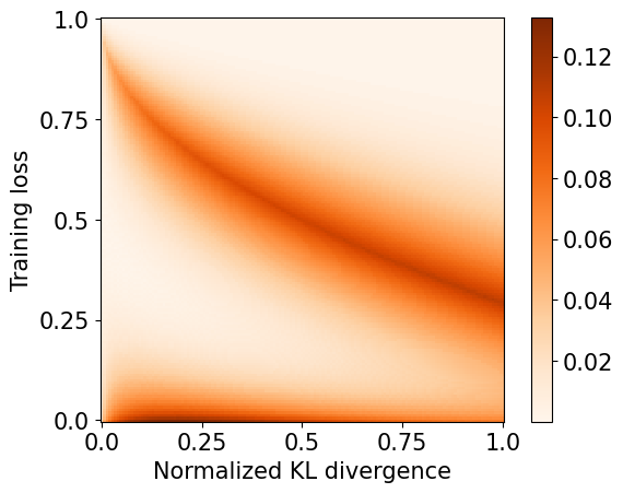
(a) The difference between the binary KL bound on the population loss and the one obtained via sub-Gaussianity for a bounded loss function.

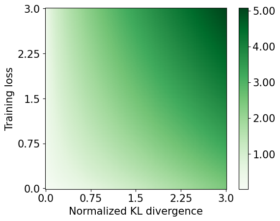
(b) The difference between the sub-Poissonian bound on the population loss obtained via 48 and the one obtained via 45.

Figure 1: Numerical evaluations for Section 5.

To begin, we consider sub-Bernoulli losses—that is, bounded losses. As mentioned, the Cramér function in this case is the binary KL divergence $\mathrm{kl}(q,p)$, while the difference comparator $\Delta_{t}(q,p)$ leads to the sub-Gaussian bound (since bounded losses are $1/2$-sub-Gaussian). To compare these bounds, we evaluate

$$\min\big{\{}1,\big{(}\alpha+\sqrt{\beta/2n}\big{)}\big{\}}-\widehat{B}^{\mathrm{kl}}_{n}(\alpha,\beta,1),$$ (60)

where $\alpha$ is the training loss and $\beta/n$ is the normalized KL divergence. This is illustrated in Fig. 1(a). When both $\alpha$ and $\beta$ are high, both bounds lead to the trivial upper bound of $1$, and are thus equal. The binary KL bound is most clearly advantageous for small training losses and in the region where the sub-Gaussian bound becomes trivial.

In Fig. 1(b), we consider sub-Poissonian losses, and numerically evaluate the discrepancy between the bound based on 45 and the one based on 48, that is,

$$\inf_{t}\big{\{}\widehat{B}^{\Delta_{t}}_{n}(\alpha,\beta,\Upsilon^{\mathcal{P}}_{\Delta_{t}})\big{\}}-\widehat{B}^{\Delta^{\Psi}_{\mathcal{P}_{\textrm{Poi}}}}_{n}(\alpha,\beta,1).$$ (61)

Since 45 is optimal, 61 is non-negative for all values. The biggest discrepancy arises when the training loss and the normalized KL divergence are both high. If one removes the minimum in 60, the same behavior emerges for bounded losses (see Section C.2).

For sub-gamma losses, it is unclear how to construct an alternative comparator. Indeed, for any comparator based on a scaled difference of population and training loss, the CGF depends on the true mean, and is unbounded when taking the supremum. One approach, taken by Germain et al., (2016), is to assume that both parameters of the bounding distribution, and hence its mean, are bounded. However, this necessitates stronger assumptions on the true loss distribution. In light of this discussion, we simply present the values of the bound based on 52 in Section C.2, where we also evaluate bounds for other bounding distributions and study the $n$-dependence of the bounds based on the Cramér function. Code for reproducing all of our figures is available at https://bit.ly/comparators.

6 Discussion and Outlook

In this paper, we studied the optimal comparator function for generalization bounds under CGF constraints. For PAC-Bayesian bounds, we showed that the bounds in terms of the Cramér function are near-optimal up to a logarithmic term. Whether or not this term can be removed remains an open question which, as discussed by Foong et al., (2021), is relevant for the small-data regime. Furthermore, the use of almost exchangeable priors, which gives rise to average bounds in terms of the conditional mutual information, has proven fruitful to obtain tighter bounds for bounded losses (Audibert,, 2004; Catoni,, 2007; Steinke and Zakynthinou,, 2020; Haghifam et al.,, 2022), with some work on improving comparators (Hellström and Durisi,, 2022). Combining this with our techniques may shed further light on the comparator choice. Finally, while we considered generalization bounds under CGF constraints, this precludes heavy-tailed losses. Extending our analysis to generalization bounds under moment constraints, for instance, is a promising avenue for future studies.

Acknowledgements

F.H. acknowledges support by the Wallenberg AI, Autonomous Systems and Software Program (WASP) funded by the Knut and Alice Wallenberg Foundation. B.G. acknowledges partial support by the U.S. Army Research Laboratory and the U.S. Army Research Office, and by the U.K. Ministry of Defence and the U.K. Engineering and Physical Sciences Research Council (EPSRC) under grant number EP/R013616/1, and partial support from the French National Agency for Research, grants ANR-18-CE40-0016-01 and ANR-18-CE23-0015-02.

Appendix A Useful Facts

In this section, we summarize the main notation used in the paper and provide some relevant background.

A.1 Summary of Notation

Notation	Definition	First use
${Q_{n}}$ and $Q_{0}$	Posterior and prior	page 1
${\mathbb{L}}\subseteq{\mathbb{R}}^{+}$	Loss range	page 2
$R_{\,{\mathbf{z}}}(h)$	$\frac{1}{n}\sum_{i=1}^{n}\ell(h,{\textnormal{z}}_{i})$	1
${R}_{D}(h)$	$\mathbb{E}_{{\textnormal{h}},{\mathbf{z}}\sim{Q_{n}}D^{n}}[{R}_{D}({\textnormal{h}})]$	2
$\bar{R}_{{\mathbf{z}}}({Q_{n}})$	$\mathbb{E}_{{\textnormal{h}}\sim{Q_{n}}}[R_{\,{\mathbf{z}}}({\textnormal{h}})]$	3
$\bar{R}_{D}({Q_{n}})$	$\mathbb{E}_{{\textnormal{h}}\sim{Q_{n}}}[{R}_{D}({\textnormal{h}})]$	4
$\Upsilon_{\Delta}(n)$	$\sup_{r\in[0,1]}\sum_{k=0}^{n}\binom{n}{k}r^{k}(1-r)^{n-k}e^{n\Delta(k/n,r)}$	6
$B^{\Delta}_{n}(\alpha,\beta,\iota)$	$\sup_{\rho\in{\mathbb{L}}}\big{\{}\rho:\Delta(\alpha,\rho)\leq\frac{\beta+\ln\frac{\iota(n)}{\delta}}{n}\big{\}}$	7
$\widehat{R}_{{\mathbf{z}}}({Q_{n}})$	$\mathbb{E}_{{\textnormal{h}},{\mathbf{z}}\sim{Q_{n}}D^{n}}[R_{\,{\textnormal{z}}}({\textnormal{h}})]$	15
$\widehat{R}_{D}({Q_{n}})$	$\mathbb{E}_{{\textnormal{h}},{\mathbf{z}}\sim{Q_{n}}D^{n}}[{R}_{D}({\textnormal{h}})]$	16
$\Upsilon^{\mathcal{P}}_{\Delta}(n)$	$\sup_{r\in{\mathbb{L}}}\mathbb{E}_{\,{\mathbf{x}}\sim P_{r}^{n}}\exp\!\left({n\Delta(\bar{\mathbf{x}},r)}\right)$	Thm. 2
$\Psi_{p}(t)$	$\ln\mathbb{E}_{X\sim P_{p}}[e^{tX}]$	Thm. 4
$\Delta^{\Psi}_{\mathcal{P}}(q,p)$	$\Psi_{p}^{*}(q)=\sup_{t\in\mathcal{T}_{p}}\big{\{}tq-\Psi_{p}(t)\big{\}}$	24
$\widehat{B}^{\Delta}_{n}(\alpha,\beta,\iota)$	$\sup_{\rho\in{\mathbb{L}}}\big{\{}\rho:\Delta(\alpha,\rho)\leq\frac{\beta+\ln\iota(n)}{n}\big{\}}$	25
$\bar{\Upsilon}(\mathcal{P})$	$\Upsilon^{\mathcal{P}}_{\Delta^{\Psi}_{\mathcal{P}}}$	Thm. 8
$\Xi$	$\pi^{2}(1+\min\{\bar{R}_{{\mathbf{z}}}({Q_{n}}),\mathrm{KL}({Q_{n}}\|Q_{0})\})^{2}/3$	41
$\Phi_{q}(r)$	$-\Psi_{r}(q)$	78
$A$	$\sup_{c_{q},c_{p}\in{\mathbb{R}}}\big{\{}-\Delta^{*}(c_{q},c_{p})+\Phi^{*}_{c_{q}}(c_{p})\big{\}}$	87

Table 1: Summary of notation.

For reference, in Table 1, we summarize the main notation used throughout the main text and the appendix.

A.2 Information Theory

We begin by providing some definitions and results from information theory. More details are available, for instance, in Cover and Thomas, (2006). First, we provide the definition of the KL divergence.

Definition 16 (KL divergence).

Let $P$ and $Q$ be two distributions such that $P\ll Q$. Then, the KL divergence between $P$ and $Q$ is, with $\ln\frac{\mathrm{d}P}{\mathrm{d}Q}$ denoting the Radon-Nikodym derivative,

$$\mathrm{KL}(P\|Q)=\int\mathrm{d}P\ln\frac{\mathrm{d}P}{\mathrm{d}Q}.$$ (62)

Note that the KL divergence is non-negative, i.e., $\mathrm{KL}(P\|Q)\geq 0$.

If x and y are random variables with joint distribution $P_{{\textnormal{x}}{\textnormal{y}}}$ and product of marginals $P_{\textnormal{x}}P_{\textnormal{y}}$, $\mathrm{KL}(P_{{\textnormal{x}}{\textnormal{y}}}\|P_{\textnormal{x}}P_{\textnormal{y}})=\mathrm{I}({\textnormal{x}};{\textnormal{y}})$ is the mutual information between x and y. The chain rule of mutual information states that, with a third random variable z, $\mathrm{I}({\textnormal{x}};{\textnormal{y}},{\textnormal{z}})=\mathrm{I}({\textnormal{x}};{\textnormal{z}})+\mathrm{I}({\textnormal{x}};{\textnormal{y}}|{\textnormal{z}})$, where $\mathrm{I}({\textnormal{x}};{\textnormal{y}}|{\textnormal{z}})$ is the conditional mutual information. If z is independent of either x or y, we have $\mathrm{I}({\textnormal{x}};{\textnormal{y}})\leq\mathrm{I}({\textnormal{x}};{\textnormal{y}}|{\textnormal{z}})$.

A cornerstone of information-theoretic and PAC-Bayesian analysis is the Donsker-Varadhan variational representation of the KL divergence (Donsker and Varadhan,, 1975).

Lemma 17 (Donsker-Varadhan variational representation).

Let $Q$ be a probability distribution on a measurable space ${\mathbb{X}}$, and let $\Pi$ denote the set of probability measures such that, for all $P\in\Pi$, we have $P\ll Q$. For every measurable function $f:{\mathbb{X}}\rightarrow{\mathbb{R}}$ such that $\mathbb{E}_{{\textnormal{x}}\sim Q}[e^{f({\textnormal{x}})}]<\infty$, we have

$$\ln\mathbb{E}_{{\textnormal{x}}\sim Q}[e^{f({\textnormal{x}})}]=\sup_{P\in\Pi}\bigg{\{}\mathbb{E}_{{\textnormal{x}}\sim P}[f({\textnormal{x}})]-\mathrm{KL}(P\|Q)\bigg{\}}.$$ (63)

The supremum is attained by the Gibbs distribution $G$, which for any measurable $\mathcal{E}\subset{\mathbb{X}}$ is given by

$$\mathrm{d}G(\mathcal{E})=\frac{\int_{\mathcal{E}}e^{f(x)}\mathrm{d}Q(x)}{\mathbb{E}_{{\textnormal{x}}\sim Q}[e^{f({\textnormal{x}})}]}.$$ (64)

Finally, we present the golden formula for mutual information (Csiszar and Körner,, 2011, Eq. 8.7).

Lemma 18 (Golden formula for mutual information).

Consider two random variables x on ${\mathbb{X}}$ and y on ${\mathbb{Y}}$ with joint distribution $P_{{\textnormal{x}}{\textnormal{y}}}$ and marginal distributions $P_{\textnormal{x}}$ and $P_{\textnormal{y}}$. Let $Q_{\textnormal{x}}$ be a distribution on ${\mathbb{X}}$, such that ${\textnormal{x}}\sim Q_{\textnormal{x}}$ is independent of y. Then,

$$\mathrm{I}({\textnormal{x}};{\textnormal{y}})=\mathrm{KL}(P_{{\textnormal{x}}{\textnormal{y}}}\|P_{\textnormal{x}}P_{\textnormal{y}})\leq\mathrm{KL}(P_{{\textnormal{x}}{\textnormal{y}}}\|Q_{\textnormal{x}}P_{\textnormal{y}}).$$ (65)

A.3 Convex Analysis

The convex conjugate of a function $f:{\mathbb{X}}\rightarrow{\mathbb{Y}}$ is defined as

$$f^{*}({\bm{y}})=\sup_{{\bm{x}}\in{\mathbb{X}}}\big{\{}\langle{\bm{x}},{\bm{y}}\rangle-f({\bm{x}})\big{\}},$$ (66)

where $\langle\cdot,\cdot\rangle$ is the inner product. The convex conjugate of any function is convex and lower semicontinuous. Recall that $\mathcal{C}$ denotes the set of functions that are convex, proper, and lower semicontinuous. For $f\in\mathcal{C}$, $(f^{*})^{*}=f$. The convex conjugate is order-reversing in the following sense: if, for two functions $f$ and $g$, we have $f({\bm{x}})\leq g({\bm{x}})$ for all ${\bm{x}}\in{\mathbb{X}}$, we have $f^{*}({\bm{y}})\geq g^{*}({\bm{y}})$ for all ${\bm{y}}\in{\mathbb{Y}}$. For a more comprehensive overview, see Rockafellar, (1970).

A.4 Natural Exponential Families

An natural exponential family (NEF) is a set of probability distributions whose probability density (or mass) functions can be written

$$p(x|\theta)=h(x)e^{\theta x-g(\theta)},$$ (67)

where $h(x)$ and $g(\theta)$ are known functions and $\theta$ is the natural parameter. The function $g(\theta)$ is referred to as the log-normalizer. The CGF for a distribution $P$ in a NEF is given by

$$\Psi_{P}(t)=\ln\mathbb{E}_{{\textnormal{x}}\sim P}[e^{t{\textnormal{x}}}]=g(\theta+t)-g(\theta).$$ (68)

This implies that the mean can be computed as $g^{\prime}(\theta)$. Further details are available in Nielsen and Garcia, (2009) and Wasserman, (2010, Sec. 9.13.3).

Appendix B Proofs

In this section, we provide the proofs of all results from the main text. For convenience, we repeat the statement of each result prior to proving it, demarcated by a horizontal rule on the left side. Note that the equation numbering in these repetitions coincides with the numbering used in the main text, to avoid any possible confusion.

B.1 Proofs for Section 2

See 2

Proof.

As $\Delta$ is convex, Jensen’s inequality implies that

$$\Delta(\widehat{R}_{{\mathbf{z}}}({Q_{n}}),\widehat{R}_{D}({Q_{n}}))\leq\mathbb{E}_{{\textnormal{h}},{\mathbf{z}}\sim{Q_{n}}D^{n}}\big{[}\Delta(R_{\,{\mathbf{z}}}({\textnormal{h}}),{R}_{D}({\textnormal{h}}))\big{]}.$$ (69)

Next, we use the Donsker-Varadhan variational representation of the KL divergence (Lemma 17) to obtain

$$\mathbb{E}_{{\textnormal{h}},{\mathbf{z}}\sim{Q_{n}}D^{n}}\big{[}\Delta(R_{\,{\mathbf{z}}}({\textnormal{h}}),{R}_{D}({\textnormal{h}}))\big{]}\leq\frac{\mathrm{KL}({Q_{n}}D^{n}\|Q_{0}D^{n})+\ln\mathbb{E}_{{\textnormal{h}},{\mathbf{z}}\sim Q_{0}D^{n}}\big{[}e^{n\Delta(R_{\,{\mathbf{z}}}({\textnormal{h}}),{R}_{D}({\textnormal{h}}))}\big{]}}{n}.$$ (70)

Next, we replace the expectation over the prior by the supremum:

$$\ln\mathbb{E}_{{\textnormal{h}},{\mathbf{z}}\sim Q_{0}D^{n}}\big{[}e^{n\Delta(R_{\,{\mathbf{z}}}({\textnormal{h}}),{R}_{D}({\textnormal{h}}))}\big{]}\leq\sup_{h\in\mathcal{H}}\ln\big{[}\mathbb{E}_{{\mathbf{z}}\sim D^{n}}e^{n\Delta(R_{\,{\mathbf{z}}}(h),{R}_{D}(h))}\big{]}.$$ (71)

By the assumption that $\Delta\in\mathcal{F}$, we have

$$\sup_{h\in\mathcal{H}}\ln\mathbb{E}_{{\mathbf{z}}\sim D^{n}}\big{[}e^{n\Delta(R_{\,{\mathbf{z}}}(h),{R}_{D}(h))}\big{]}\leq\sup_{h\in\mathcal{H}}\ln\mathbb{E}_{{\mathbf{r}}^{\prime}_{h}\sim P_{{R}_{D}(h)}^{n}}\big{[}e^{n\Delta(\bar{{\mathbf{r}}}^{\prime}_{h},{R}_{D}(h))}\big{]}.$$ (72)

Finally, as the highest population loss is no greater than the highest loss, we get

$$\sup_{h\in\mathcal{H}}\ln\mathbb{E}_{{\mathbf{r}}^{\prime}_{h}\sim P_{{R}_{D}(h)}^{n}}\big{[}e^{n\Delta(\bar{{\mathbf{r}}}^{\prime}_{h},{R}_{D}(h))}\big{]}\leq\sup_{r\in{\mathbb{L}}}\ln\mathbb{E}_{{\mathbf{x}}\sim P_{r}^{n}}\big{[}e^{n\Delta(\bar{{\mathbf{x}}},r)}\big{]}.$$ (73)

The result follows by combining 69 to 73. ∎

See 4

Proof.

We begin by proving the upper bound in 26. First, we use the fact that the moment-generating function for a sum of independent random variables factorizes, so that

$$\mathbb{E}_{{\mathbf{x}}\sim P_{p}^{n}}[e^{nt\bar{{\mathbf{x}}}}]=\left(\mathbb{E}_{{\textnormal{x}}\sim P_{p}}[e^{t{\textnormal{x}}}]\right)^{n}.$$ (74)

By definition, for any fixed $t$, we have

$$\mathbb{E}_{{\textnormal{x}}\sim P_{p}}[e^{t{\textnormal{x}}-\Psi_{p}(t)}]=1.$$ (75)

Hence, we find that with $\Delta(q,p)=tq-\Psi_{p}(t)$ for any fixed $t\in\mathcal{T}$, we have

$$t\widehat{R}_{{\mathbf{z}}}({Q_{n}})-\Psi_{\widehat{R}_{D}({Q_{n}})}(t)\leq\frac{\mathrm{KL}({Q_{n}}D^{n}\|Q_{0}D^{n})}{n}.$$ (76)

Since this holds for any $t\in\mathcal{T}$, it also holds for the supremum. Hence,

$$\Delta^{\Psi}_{\mathcal{P}}(\widehat{R}_{{\mathbf{z}}}({Q_{n}}),\widehat{R}_{D}({Q_{n}}))=\sup_{t\in\mathcal{T}}\big{\{}t\widehat{R}_{{\mathbf{z}}}({Q_{n}})-\Psi_{\widehat{R}_{D}({Q_{n}})}(t)\big{\}}\leq\frac{\mathrm{KL}({Q_{n}}D^{n}\|Q_{0}D^{n})}{n}.$$ (77)

This establishes 26.

We now turn to proving the lower bound in 27. To do this, we will show that, for any choice of $\Delta$ in Theorem 2, the resulting bound on $\widehat{R}_{D}({Q_{n}})$ is no better than the stated lower bound. The proof consists of three steps: (i) lower-bounding $\Upsilon^{\mathcal{P}}_{\Delta}$, (ii) upper-bounding $\Delta$, and (iii) putting every thing together. This roughly follows along the same lines as the proof of Foong et al., (2021, Thm. 4), with key modifications and subtleties that arise due to considering unbounded loss functions. For convenience, we introduce

$$\Phi_{q}(r)=-\Psi_{r}(q).$$ (78)

(i): Lower-bounding $\Upsilon^{\mathcal{P}}_{\Delta}$.
Since $\Delta$ is in $\mathcal{C}$, we have

$$\Delta(q,p)=\Delta^{**}(q,p)=\sup_{c_{q},c_{p}\in{\mathbb{R}}}(c_{q}q+c_{p}p-\Delta^{*}(c_{q},c_{p})).$$ (79)

Recall that $\bar{{\mathbf{x}}}=\frac{1}{n}\sum_{i=1}^{n}{\textnormal{x}}_{i}$. Then, we have

$$\Upsilon^{\mathcal{P}}_{\Delta}(n) =\sup_{r\in{\mathbb{L}}}\mathbb{E}_{{\mathbf{x}}\sim P_{r}^{n}}e^{n\Delta(\bar{{\mathbf{x}}},r)}$$ (80)

$$=\sup_{r\in{\mathbb{L}}}\mathbb{E}_{{\mathbf{x}}\sim P_{r}^{n}}e^{\sup_{c_{q},c_{p}\in{\mathbb{R}}}(c_{q}\sum_{i}{\textnormal{x}}_{i}+nc_{p}r-n\Delta^{*}(c_{q},c_{p}))}$$ (81)

$$\geq\sup_{r\in{\mathbb{L}},c_{q},c_{p}\in{\mathbb{R}}}e^{nc_{p}r-n\Delta^{*}(c_{q},c_{p})}\mathbb{E}_{{\mathbf{x}}\sim P_{r}^{n}}e^{c_{q}\sum_{i}{\textnormal{x}}_{i}}$$ (82)

$$=\sup_{r\in{\mathbb{L}},c_{q},c_{p}\in{\mathbb{R}}}e^{nc_{p}r-n\Delta^{*}(c_{q},c_{p})}\exp\left(n\Psi_{r}(c_{q})\right)$$ (83)

$$=\sup_{r\in{\mathbb{L}},c_{q},c_{p}\in{\mathbb{R}}}e^{nc_{p}r-n\Delta^{*}(c_{q},c_{p})}\exp\left(-n\Phi_{c_{q}}(r)\right).$$ (84)

Hence, we obtain

$$\frac{\ln\Upsilon^{\mathcal{P}}_{\Delta}(n)}{n} \geq\sup_{c_{q},c_{p}\in{\mathbb{R}}}\big{\{}-\Delta^{*}(c_{q},c_{p})+\sup_{r\in{\mathbb{L}}}\big{[}c_{p}r-\Phi_{c_{q}}(r)\big{]}\big{\}}$$ (85)

$$=\sup_{c_{q},c_{p}\in{\mathbb{R}}}\big{\{}-\Delta^{*}(c_{q},c_{p})+\Phi^{*}_{c_{q}}(c_{p})\big{\}}$$ (86)

$$:=A.$$ (87)

Note that, since $\Delta$ is proper, $A$ is finite.

(ii): Upper-bounding $\Delta$.
Define $\tilde{\Delta}^{*}$ as

$$\tilde{\Delta}^{*}(c_{p},c_{q})=-A+\Phi^{*}_{c_{q}}(c_{p}).$$ (88)

Since $A$ is finite, $\tilde{\Delta}^{*}$ is proper. Furthermore, as it is an affine transformation of a convex conjugate, it is convex and lower semicontinuous. Hence, $\tilde{\Delta}^{*}\in\mathcal{C}$, which implies that $(\tilde{\Delta}^{*})^{**}=\tilde{\Delta}^{*}$. This motivates the notation $\tilde{\Delta}=(\tilde{\Delta}^{*})^{*}$. With this, we obtain

$$\tilde{\Delta}(q,p) =A+\sup_{c_{p},c_{q}\in{\mathbb{R}}}[c_{q}q+c_{p}p-\Phi^{*}_{c_{q}}(c_{p})]$$ (89)

$$=A+\sup_{c_{q}\in{\mathbb{R}}}[c_{q}q+\Phi_{c_{q}}(p)]$$ (90)

$$=A+\sup_{c_{q}\in{\mathbb{R}}}[c_{q}q-\Psi_{p}(c_{q})]$$ (91)

$$=A+\Psi_{p}^{*}(q).$$ (92)

We now need to show that $\tilde{\Delta}(q,p)\geq\Delta(q,p)$ for all $q,p\in{\mathbb{L}}$:

$$-\tilde{\Delta}^{*}(c_{q},c_{p})+\Phi^{*}_{c_{q}}(c_{p}) =A$$ (93)

$$=\sup_{c_{q},c_{p}\in{\mathbb{R}}}\big{\{}-\Delta^{*}(c_{q},c_{p})+\Phi^{*}_{c_{q}}(c_{p})\big{\}}$$ (94)

$$\geq-\Delta^{*}(c_{q},c_{p})+\Phi^{*}_{c_{q}}(c_{p}).$$ (95)

Therefore, we have $\tilde{\Delta}^{*}\leq\Delta^{*}$, which implies $\tilde{\Delta}\geq\Delta$ by the order-reversing property of the convex conjugate.

(iii): Putting everything together.
First, since $\tilde{\Delta}\geq\Delta$, we have

$$\widehat{B}^{\tilde{\Delta}}_{n}(\bar{R}_{{\mathbf{z}}}({Q_{n}}),\mathrm{KL}({Q_{n}}\|Q_{0}),\Upsilon^{\mathcal{P}}_{\Delta})\leq\widehat{B}^{\Delta}_{n}(\bar{R}_{{\mathbf{z}}}({Q_{n}}),\mathrm{KL}({Q_{n}}\|Q_{0}),\Upsilon^{\mathcal{P}}_{\Delta}).$$ (96)

Furthermore, since $\ln\big{(}\Upsilon^{\mathcal{P}}_{\Delta}(n)\big{)}/n\geq A$, we have

$$\widehat{B}^{\tilde{\Delta}}_{n}(\bar{R}_{{\mathbf{z}}}({Q_{n}}),\mathrm{KL}({Q_{n}}\|Q_{0}),e^{nA})\leq\widehat{B}^{\tilde{\Delta}}_{n}(\bar{R}_{{\mathbf{z}}}({Q_{n}}),\mathrm{KL}({Q_{n}}\|Q_{0}),\Upsilon^{\mathcal{P}}_{\Delta}).$$ (97)

Finally, since $\tilde{\Delta}(q,p)=A+\Psi_{p}^{*}(q)=A+\Delta^{\Psi}_{\mathcal{P}}(q,p)$, we obtain

$$\widehat{B}^{\tilde{\Delta}}_{n}(\bar{R}_{{\mathbf{z}}}({Q_{n}}),\mathrm{KL}({Q_{n}}\|Q_{0}),e^{nA})=\widehat{B}^{\Delta^{\Psi}_{\mathcal{P}}}_{n}(\bar{R}_{{\mathbf{z}}}({Q_{n}}),\mathrm{KL}({Q_{n}}\|Q_{0}),1),$$ (98)

leading to the final lower bound.

∎

See 5

Proof.

For completeness, we begin by proving Kullback’s inequality (Kullback,, 1954). Let $P$ and $Q$ be two distributions such that $P\ll Q$. Let $Q_{\alpha}$ be defined so that, for every measurable set $\mathcal{E}$,

$$Q_{\alpha}(\mathcal{E})=\frac{\int_{\mathcal{E}}e^{\alpha x}Q(dx)}{\int_{\mathbb{R}}e^{\alpha x}Q(dx)}=\frac{1}{M_{Q}(\alpha)}\int_{\mathcal{E}}e^{\alpha x}Q(dx),$$ (99)

where $M_{Q}(\alpha)$ denotes the moment-generating function of $Q$. Then, we find that

$$\mathrm{KL}(P\|Q) =\int_{\mathbb{R}}\mathrm{d}P\ln\left(\frac{\mathrm{d}Q}{\mathrm{d}P}\right)$$ (100)

$$=\int_{\mathbb{R}}\mathrm{d}P\ln\left(\frac{\mathrm{d}Q}{\mathrm{d}P}\frac{\mathrm{d}Q_{\alpha}}{\mathrm{d}Q_{\alpha}}\right)$$ (101)

$$=\mathrm{KL}(P\|Q_{\alpha})+\int_{\mathbb{R}}\mathrm{d}P\ln\left(\frac{\mathrm{d}Q_{\alpha}}{\mathrm{d}Q}\right).$$ (102)

The last term can be decomposed as

$$\int_{\mathbb{R}}\mathrm{d}P\ln\left(\frac{\mathrm{d}Q_{\alpha}}{\mathrm{d}Q}\right) =\int_{\mathbb{R}}\mathrm{d}P\ln\left(\frac{e^{\alpha x}}{M_{Q}(\alpha)}\right)$$ (103)

$$=\alpha\mu_{P}-\Psi_{Q}(\alpha),$$ (104)

where $\mu_{P}$ denotes the first moment of $P$ and $\Psi_{Q}(\alpha)$ is the CGF of $Q$. Now, due to the non-negativity of the KL divergence, we have

$$\mathrm{KL}(P\|Q) =\mathrm{KL}(P\|Q_{\alpha})+\alpha\mu_{P}-\Psi_{Q}(\alpha)$$ (105)

$$\geq\alpha\mu_{P}-\Psi_{Q}(\alpha).$$ (106)

Finally, by taking the supremum over $\alpha$, we obtain Kullback’s inequality:

$$\mathrm{KL}(P\|Q)\geq\sup_{\alpha}\big{\{}\alpha\mu_{P}-\Psi_{Q}(\alpha)\big{\}}=\Psi^{*}_{Q}(\mu_{P}).$$ (107)

To establish the desired result, we need to show that the above is an equality provided that the distributions are in the same NEF. Thus, assume that $P$ and $Q$ are in a NEF, with natural parameters $\theta_{P}$ and $\theta_{Q}$ respectively. Denote the first moment of $P$ as $p$ and the first moment of of $Q$ as $q$.

First, observe that since $Q$ is in a NEF with parameter $\theta_{Q}$, as defined in 30, the transformation in 99 gives another member of the NEF, but with parameter $\theta_{Q}+\alpha$. Since $Q$ is in a NEF, the CGF is

$$\Psi_{Q}(t)=g(\theta_{Q}+t)-g(\theta_{Q}).$$ (108)

In particular, the first moment is $q=g^{\prime}(\theta_{Q})$. Hence, the transformation in 99 leads to a distribution with first moment $g^{\prime}(\theta_{Q}+\alpha)$. If we set $\alpha=\theta_{P}-\theta_{Q}$, we thus obtain a distribution with first moment $p=g^{\prime}(\theta_{P})$—and since it is in the same NEF, $Q_{\theta_{P}-\theta_{Q}}=P$. From this, it follows that $\mathrm{KL}(P\|Q_{\theta_{P}-\theta_{Q}})=0$. Therefore, by following the same procedure as above,

$$\mathrm{KL}(P\|Q) =\mathrm{KL}(P\|Q_{\theta_{P}-\theta_{Q}})+(\theta_{P}-\theta_{Q})\mu_{P}-\Psi_{Q}(\theta_{P}-\theta_{Q})$$ (109)

$$=(\theta_{P}-\theta_{Q})\mu_{P}-\Psi_{Q}(\theta_{P}-\theta_{Q}).$$ (110)

Now, since the general upper bound of Kullback’s inequality in 107 holds, and equality is achieved with $\alpha=(\theta_{P}-\theta_{Q})$, it follows that this must be the supremum over $\alpha$. Thus, we conclude

$$\mathrm{KL}(P\|Q) =\sup_{\alpha}\big{\{}\alpha\mu_{P}-\Psi_{Q}(\alpha)\big{\}}$$ (111)

$$=\Psi_{Q}^{*}(\mu_{P}).$$ (112)

∎

See 6

Proof.

As in the proof of Theorem 2, we begin by using the convexity of $\Delta$ and Jensen’s inequality to conclude that

$$\Delta(\widehat{R}_{{\mathbf{z}}}({Q_{n}}),\widehat{R}_{D}({Q_{n}}))\leq\mathbb{E}_{{\textnormal{h}},{\mathbf{z}}\sim{Q_{n}}D^{n}}\big{[}\Delta(R_{\,{\mathbf{z}}}({\textnormal{h}}),{R}_{D}({\textnormal{h}}))\big{]}.$$ (113)

Now, recall that $R_{\,{\mathbf{z}}}({\textnormal{h}})=\frac{1}{n}\sum_{i=1}^{n}\ell({\textnormal{h}},{\textnormal{z}}_{i})$. Thus, by using Jensen’s inequality again,

$$\mathbb{E}_{{\textnormal{h}},{\mathbf{z}}\sim{Q_{n}}D^{n}}\big{[}\Delta(R_{\,{\mathbf{z}}}({\textnormal{h}}),{R}_{D}({\textnormal{h}}))\big{]}\leq\mathbb{E}_{{\textnormal{h}},{\mathbf{z}}\sim{Q_{n}}D^{n}}\bigg{[}\frac{1}{n}\sum_{i=1}^{n}\Delta(\ell({\textnormal{h}},{\textnormal{z}}_{i}),{R}_{D}({\textnormal{h}}))\bigg{]}.$$ (114)

By the linearity of expectation and marginalizing,

$$\mathbb{E}_{{\textnormal{h}},{\mathbf{z}}\sim{Q_{n}}D^{n}}\bigg{[}\frac{1}{n}\sum_{i=1}^{n}\Delta(\ell({\textnormal{h}},{\textnormal{z}}_{i}),{R}_{D}({\textnormal{h}}))\bigg{]}=\frac{1}{n}\sum_{i=1}^{n}\mathbb{E}_{{\textnormal{h}},{\textnormal{z}}_{i}\sim{Q_{i}}D^{n}}\big{[}\Delta(\ell({\textnormal{h}},{\textnormal{z}}_{i}),{R}_{D}({\textnormal{h}}))\big{]}.$$ (115)

The proof now essentially proceeds as in Theorem 2, but for each term in the sum. First, by using the Donsker-Varadhan variational representation of the KL divergence (Lemma 17), we obtain

$$\mathbb{E}_{{\textnormal{h}},{\textnormal{z}}_{i}\sim{Q_{n}}D}\big{[}\Delta(\ell({\textnormal{h}},{\textnormal{z}}_{i}),{R}_{D}({\textnormal{h}}))\big{]}\leq\mathrm{KL}({Q_{i}}D\|Q_{0}D)+\ln\mathbb{E}_{{\textnormal{h}},{\textnormal{z}}_{i}\sim Q_{0}D}\big{[}e^{\Delta(\ell({\textnormal{h}},{\textnormal{z}}_{i}),{R}_{D}({\textnormal{h}}))}\big{]}.$$ (116)

By replacing the expectation over the prior by the supremum, using the assumption that $\Delta\in\mathcal{F}$, and the fact that the highest population loss is no greater than the highest loss, we get

$$\ln\mathbb{E}_{{\textnormal{h}},{\textnormal{z}}_{i}\sim Q_{0}D}\big{[}e^{\Delta(\ell({\textnormal{h}},{\textnormal{z}}_{i}),{R}_{D}({\textnormal{h}}))}\big{]}\leq\sup_{r\in{\mathbb{L}}}\ln\mathbb{E}_{{\textnormal{x}}\sim P_{r}}\big{[}e^{\Delta({\textnormal{x}},r)}\big{]}.$$ (117)

The result follows by combining 113 to 117. ∎

B.2 Proofs for Section 3

See 7

Proof.

The proof essentially follows the same lines as Theorem 2, with an additional application of Markov’s inequality. Recall that $\bar{{\mathbf{x}}}=\frac{1}{n}\sum_{i=1}^{n}{\textnormal{x}}_{i}$. Then, by Jensen’s inequality and the Donsker-Varadhan variational representation (Lemma 17),

$$\Delta(\bar{R}_{{\mathbf{z}}}({Q_{n}}),\bar{R}_{D}({Q_{n}})) \leq\mathbb{E}_{{\textnormal{h}}\sim{Q_{n}}}\big{[}\Delta(R_{\,{\mathbf{z}}}({\textnormal{h}}),{R}_{D}({\textnormal{h}}))\big{]}$$ (118)

$$\leq\frac{\mathrm{KL}({Q_{n}}\|Q_{0})+\ln\mathbb{E}_{{\textnormal{h}}\sim Q_{0}}\big{[}e^{n\Delta(R_{\,{\mathbf{z}}}({\textnormal{h}}),{R}_{D}({\textnormal{h}}))}\big{]}}{n}.$$ (119)

Now, by Markov’s inequality, we have that with probability $1-\delta$,

$$\ln\mathbb{E}_{{\textnormal{h}}\sim Q_{0}}\big{[}e^{n\Delta(R_{\,{\mathbf{z}}}({\textnormal{h}}),{R}_{D}({\textnormal{h}}))}\big{]}\leq\ln\bigg{(}\frac{1}{\delta}\mathbb{E}_{{\textnormal{h}}\sim Q_{0},{\mathbf{z}}\sim D^{n}}\big{[}e^{n\Delta(R_{\,{\mathbf{z}}}({\textnormal{h}}),{R}_{D}({\textnormal{h}}))}\big{]}\bigg{)}.$$ (120)

The remaining steps are identical to 71 to 73, after which the result follows. ∎

See 8

Proof.

We begin with 36. The proof of 27, for the average case in Theorem 4, can be applied verbatim in the PAC-Bayesian case, as it is only concerned with the structure of $\Delta$ and $\Upsilon^{\mathcal{P}}_{\Delta}(n)$. As these are identical in Theorem 8, the exact same argument can be used, with $B$ in place of $\widehat{B}$ in 96 to 98.

Next, the result in 37 follows immediately from Theorem 7 by setting $\Delta$ to $\Delta^{\Psi}_{\mathcal{P}}$.

We now turn to 38. By definition, for any fixed $t$, we have

$$\mathbb{E}_{{\textnormal{x}}\sim P_{p}}[e^{t\bar{{\textnormal{x}}}-\Psi_{p}(t)}]=1.$$ (121)

Hence, we find that with $\Delta(q,p)=tq-\Psi_{p}(t)$ for any fixed $t\in\mathcal{T}$, with probability $1-\delta$,

$$t\bar{R}_{{\mathbf{z}}}({Q_{n}})-\Psi_{\bar{R}_{D}({Q_{n}})}(t)\leq\frac{\mathrm{KL}({Q_{n}}\|Q_{0})+\ln\frac{1}{\delta}}{n}.$$ (122)

This establishes 38.

∎

See 9

Proof.

The proofs of these upper bounds are similar to the average case in Theorem 4, but as we are dealing with a probabilistic result, we need to apply carefully constructed union bounds.

We begin with 39. We will consider the situations where the KL divergence and the training loss are bounded separately, and we begin with the KL case. Now, note that the supremum over $t$ in 122 is achieved for a $t>0$ (Boucheron et al.,, 2013, Sec. 2.2). Hence, we can recast 122 as

$$\bar{R}_{{\mathbf{z}}}({Q_{n}})\leq\frac{\mathrm{KL}({Q_{n}}\|Q_{0})+\ln\frac{1}{\delta}}{nt}+\frac{\Psi_{\bar{R}_{D}({Q_{n}})}(t)}{t}.$$ (123)

We now wish to take the infimum over $t$ in the right-hand side in 123, which corresponds to taking the supremum over $t$ in the left-hand side of 122.

As per our assumption, we have $\mathrm{KL}({Q_{n}}\|Q_{0})\leq u(n)$. Let ${\textnormal{k}}=\lceil\mathrm{KL}({Q_{n}}\|Q_{0})\rceil$. We now follow an approach similar to Rodríguez-Gálvez et al., (2023). Specifically, 123 implies

$$\bar{R}_{{\mathbf{z}}}({Q_{n}}) \leq\frac{{\textnormal{k}}+\ln\frac{1}{\delta}}{nt}+\frac{\Psi_{\bar{R}_{D}({Q_{n}})}(t)}{t}.$$ (124)

Now, conditioned on any outcome ${\textnormal{k}}=k^{\prime}$, we can take the infimum over $t$ in the right-hand side of 124:

$$\bar{R}_{{\mathbf{z}}}({Q_{n}})\leq\inf_{t}\left\{\frac{k^{\prime}+\ln\frac{1}{\delta}}{nt}+\frac{\Psi_{\bar{R}_{D}({Q_{n}})}(t)}{t}\right\}.$$ (125)

Note that, given ${\textnormal{k}}=k^{\prime}$, we have $k^{\prime}\leq\mathrm{KL}({Q_{n}}\|Q_{0})+1$. Since the support of k is $1,\dots,\lceil u(n)\rceil$, we can apply a union bound over all possible outcomes and perform the substitution $\delta\rightarrow\delta/\lceil u(n)\rceil$ to obtain

$$\Psi_{\bar{R}_{D}({Q_{n}})}^{*}(\bar{R}_{{\mathbf{z}}}({Q_{n}}))=\sup_{t\in\mathcal{T}}\left\{t\bar{R}_{{\mathbf{z}}}({Q_{n}})-\Psi_{\bar{R}_{D}({Q_{n}})}(t)\right\}\leq\frac{\mathrm{KL}({Q_{n}}\|Q_{0})+\ln\frac{e\lceil u(n)\rceil}{\delta}}{n},$$ (126)

We now consider the case where $n\bar{R}_{{\mathbf{z}}}({Q_{n}})\leq u(n)$. Let ${\textnormal{s}}=\lceil n\bar{R}_{{\mathbf{z}}}({Q_{n}})\rceil$. We then get

$$\frac{t{\textnormal{s}}}{n}-\frac{1}{n}+\Psi_{\bar{R}_{D}({Q_{n}})}(t)\leq\frac{\mathrm{KL}({Q_{n}}\|Q_{0})+\ln\frac{1}{\delta}}{n}.$$ (127)

As for the KL divergence, we can optimize the above conditioned on any specific instance of s, which is supported on $1,\dots,\lceil u(n)\rceil$. Hence, we apply a union bound over all possible outcomes and perform the substitution $\delta\rightarrow\delta/\lceil u(n)\rceil$ to obtain

$$\Psi_{\bar{R}_{D}({Q_{n}})}^{*}(\bar{R}_{{\mathbf{z}}}({Q_{n}}))=\sup_{t\in\mathcal{T}}\left\{t\bar{R}_{{\mathbf{z}}}({Q_{n}})-\Psi_{\bar{R}_{D}({Q_{n}})}(t)\right\}\leq\frac{\mathrm{KL}({Q_{n}}\|Q_{0})+\ln\frac{e\lceil u(n)\rceil}{\delta}}{n}.$$ (128)

By combining 126 and 128 via an additional union bound, performing the substitution $\delta\rightarrow\delta/2$, we obtain 39.

We now turn to the upper bound in 40. Now, we do not assume any bound on the KL divergence or training loss, so we cannot take a union bound over a finite set. However, we can take the following approach, inspired by Seldin et al., (2012). We begin with the case where the minimum in 40 is achieved by the KL divergence, and again, we let ${\textnormal{k}}=\lceil\mathrm{KL}({Q_{n}}\|Q_{0})\rceil$. Then, as before, we have

$$\frac{\mathrm{KL}({Q_{n}}\|Q_{0})+\ln\frac{1}{\delta}}{nt}+\frac{\Psi_{\bar{R}_{D}({Q_{n}})}(t)}{t}\leq\frac{{\textnormal{k}}+\ln\frac{1}{\delta}}{nt}+\frac{\Psi_{\bar{R}_{D}({Q_{n}})}(t)}{t}.$$ (129)

Conditioned on any outcome ${\textnormal{k}}=k^{\prime}$, we can take the infimum over $t$ in the right-hand side of 129. Since ${\textnormal{k}}\in{\mathbb{N}}_{+}$, we can now take the following weighted union bound over ${\mathbb{N}}$: let $\delta\rightarrow 6\delta/(\pi^{2}k^{\prime 2})$. Note that the sum of this over $k^{\prime}$ is

$$\sum_{k^{\prime}\in{\mathbb{N}}_{+}}\frac{6\delta}{\pi^{2}k^{\prime 2}}=\delta.$$ (130)

We can thus conclude that, with probability $1-\delta$,

$$\bar{R}_{{\mathbf{z}}}({Q_{n}})\leq\inf_{t\in\mathcal{T}}\left\{\frac{\mathrm{KL}({Q_{n}}\|Q_{0})+\ln\frac{e\pi^{2}(1+\mathrm{KL}({Q_{n}}\|Q_{0}))^{2}}{6\delta}}{nt}+\frac{\Psi_{\bar{R}_{D}({Q_{n}})}(t)}{t}\right\},$$ (131)

and hence,

$$\Psi_{\bar{R}_{D}({Q_{n}})}^{*}(\bar{R}_{{\mathbf{z}}}({Q_{n}}))=\sup_{t\in\mathcal{T}}\left\{t\bar{R}_{{\mathbf{z}}}({Q_{n}})-\Psi_{\bar{R}_{D}({Q_{n}})}(t)\right\}\leq\frac{\mathrm{KL}({Q_{n}}\|Q_{0})+\ln\frac{e\pi^{2}(1+\mathrm{KL}({Q_{n}}\|Q_{0}))^{2}}{6\delta}}{n}.$$ (132)

Finally, we turn to the upper bound in terms of the training loss in 40. Let ${\textnormal{s}}=\lceil n\bar{R}_{{\mathbf{z}}}({Q_{n}})\rceil$. Again, we then get

$$\frac{t{\textnormal{s}}}{n}-\frac{1}{n}-\Psi_{\bar{R}_{D}({Q_{n}})}(t)\leq\frac{\mathrm{KL}({Q_{n}}\|Q_{0})+\ln\frac{1}{\delta}}{n}.$$ (133)

For any fixed instance of ${\textnormal{s}}=m^{\prime}\in{\mathbb{N}}_{+}$, we can take the supremum over $t$. So, taking a union bound with $\delta\rightarrow 6\delta/(\pi^{2}m^{\prime 2})$, we get

$$\Psi_{\bar{R}_{D}({Q_{n}})}^{*}(\bar{R}_{{\mathbf{z}}}({Q_{n}}))\leq\frac{\mathrm{KL}({Q_{n}}\|Q_{0})+\ln\frac{\pi^{2}(1+\bar{R}_{{\mathbf{z}}}({Q_{n}}))^{2}}{6\delta}}{n}.$$ (134)

The result in 40 follows by combining the bounds in 132 and 134 via the union bound, performing the substitution $\delta\rightarrow\delta/2$. ∎

B.3 Proofs for Section 4

See 10

Proof.

Since the Poisson distributions form a NEF, Proposition 5 implies that the Cramér function is, indeed, equal to the KL divergence in 43. Hence, 45 follows immediately from 36, while 46 follows immediately from 40. ∎

See 11

Proof.

Let ${\textnormal{x}}\sim\mathrm{Poisson}(\mu)$. Then, we have

$$\mathbb{E}[e^{(1-e^{-t})\mu-t{\textnormal{x}}}]=e^{-\mu(1-e^{-t})}e^{(1-e^{-t})\mu}=1.$$ (135)

Therefore, it follows from 18 that

$$(1-e^{-t})\widehat{R}_{D}({Q_{n}})-t\widehat{R}_{{\mathbf{z}}}({Q_{n}})\leq\frac{\mathrm{KL}({Q_{n}}D^{n}\|Q_{0}D^{n})}{n}.$$ (136)

The result follows by solving for $\widehat{R}_{D}({Q_{n}})$ and taking the infimum over $t$. ∎

See 12

Proof.

Since the gamma distributions with fixed shape parameter form a NEF, the KL divergence in 50 is the Cramér function (by Proposition 5). Hence, 52 follows immediately from 36, while 53 follows from 40. ∎

See 13

Proof.

Since the Laplace distributions do not form a NEF (unless the mean is fixed), the Cramér function cannot be computed on the basis of Proposition 5. Instead, we need to show that 55 is the Cramér function via explicit computation. To this end, note that the CGF for the distribution $\mathrm{Laplace}(b,p)$ is, for $\left\lvert t\right\rvert\leq 1/b$,

$$\Psi_{p}(t)=tp-\ln(1-b^{2}t^{2})$$ (137)

Hence, the Cramér function is

$$\Psi^{*}_{p}(q) =\sup_{\left\lvert t\right\rvert\leq 1/b}\bigg{\{}t(q-p)-\ln(1-b^{2}t^{2})\bigg{\}}$$ (138)

$$=\frac{\sqrt{(q-p)^{2}+b^{2}}}{b}-1+\ln\!\bigg{(}\frac{2(b\sqrt{(q-p)^{2}+b^{2}}-b^{2})}{(q-p)^{2}}\bigg{)},$$ (139)

where the final step follows by confirming that the maximum is attained at the critical point

$$t^{*}=\frac{\sqrt{b^{2}+(q-p)^{2}}}{b(q-p)}-\frac{1}{q-p}.$$ (140)

With this, the result follows directly from 18. ∎

See 14

Proof.

Given the form of the CGF for the distribution $\mathrm{Laplace}(b,p)$ for $\left\lvert t\right\rvert\leq 1/b$, given in 137, it follows that

$$\frac{\Upsilon^{\mathcal{P}_{\textrm{Lap}}}_{\Delta_{t}}}{n}=-\ln(1-b^{2}t^{2}).$$ (141)

Hence, it follows from 18 that

$$t(\widehat{R}_{D}({Q_{n}})-\widehat{R}_{{\mathbf{z}}}({Q_{n}}))\leq\frac{\mathrm{KL}({Q_{n}}D^{n}\|Q_{0}D^{n})}{n}-\ln(1-b^{2}t^{2}).$$ (142)

The stated result follows after division by $t$ and taking the infimum. ∎

See 15

Proof.

Given the form of the CGF, we have, for ${\textnormal{x}}\sim P_{p}$,

$$\mathbb{E}[e^{t(p-q)}]=e^{-tp+g(t^{2})}e^{tp}=e^{g(t^{2})}.$$ (143)

Thus, we conclude that

$$\frac{\Upsilon^{\mathcal{P}}_{\Delta_{t}}}{n}=g(t^{2}).$$ (144)

Therefore, it follows from 18 that, with $\alpha=\widehat{R}_{{\mathbf{z}}}({Q_{n}})$ and $\beta=\mathrm{KL}({Q_{n}}D^{n}\|Q_{0}D^{n})/n$,

$$\widehat{R}_{D}({Q_{n}})\leq\alpha+\inf_{t}\bigg{\{}\frac{\beta+g(t^{2})}{t}\bigg{\}}.$$ (145)

Note that the bound on $\widehat{R}_{D}({Q_{n}})$ 145 is the explicit form of $\inf_{t\in\mathcal{T}}\widehat{B}^{\Delta_{t}}_{n}\big{(}\alpha,\beta,\Upsilon^{\mathcal{P}}_{\Delta_{t}}\big{)}$. Now, by reorganizing 145, we obtain

$$\sup_{t\in\mathcal{T}}\big{\{}t(\alpha-\widehat{R}_{D}({Q_{n}}))-g(t^{2})\big{\}}\leq\beta.$$ (146)

Due to the assumed form of the CGF, we see that the left-hand side of 146 is indeed the Cramér function:

$$\sup_{t\in\mathcal{T}}\big{\{}t(\alpha-\widehat{R}_{D}({Q_{n}}))-g(t^{2})\big{\}}=\sup_{t\in\mathcal{T}}\big{\{}t\alpha-\big{(}t\widehat{R}_{D}({Q_{n}})+g(t^{2})\big{)}\big{\}}=\Delta^{\Psi}_{\mathcal{P}}(\alpha,\widehat{R}_{D}({Q_{n}})).$$ (147)

Hence, it implies the bound $\widehat{R}_{D}({Q_{n}})\leq\widehat{B}^{\Delta^{\Psi}_{\mathcal{P}}}_{n}\big{(}\alpha,\beta,1\big{)}$. Thus, the claimed equivalence follows. ∎

Appendix C Additional Results

In this section, we present some additional results which were not included in the main text. In Section C.1, we state and prove some theoretical results: we establish a partial characterization of $\mathcal{F}$ under the sub-$\mathcal{P}$ assumption (Proposition 19); we show that, under certain conditions, the bound in Theorem 6 always improves upon Theorem 2 (Proposition 20); and we provide some additional explicit bounds for various instances of $\mathcal{P}$ (Corollary 21). In Section C.2, we present additional numerical evaluations of the bounds to support the findings presented in Section 5.

C.1 Additional Theoretical Results

We begin with a partial characterization of $\mathcal{F}$ under the sub-$\mathcal{P}$ assumption.

Proposition 19.

Assume that $f^{\textnormal{lin}}_{t}\in\mathcal{F}$ for all $t\in{\mathbb{R}}$. Let $g:{\mathbb{L}}^{2}\rightarrow{\mathbb{R}}^{+}$ denote a function that is infinitely differentiable in its first argument. Then, $g\in\mathcal{F}$ if it is totally monotone, i.e.., for all $k\in{\mathbb{N}}$,

$$(-1)^{k}\frac{\partial^{k}e^{g(q,p)}}{\partial q^{k}}\geq 0.$$ (148)

Furthermore, $g\in\mathcal{F}$ if all of its derivatives are non-negative, i.e., for all $k\in{\mathbb{N}}$,

$$\frac{\partial^{k}e^{g(q,p)}}{\partial q^{k}}\geq 0.$$ (149)

Proof.

Consider a fixed $p$, and let $f(q)\equiv e^{g(q,p)}$. Any function that satisfies 148 is said to be totally monotone. By Bernstein’s theorem (Bernstein,, 1929), there exists a non-negative Borel measure with cumulative distribution function $\varphi$ such that

$$f(q)=\int_{0}^{\infty}e^{-tq}\varphi(t)\mathrm{d}t.$$ (150)

This implies that

$$\mathbb{E}_{{\mathbf{z}}\sim D^{n}}[f(R_{\,{\mathbf{z}}}(h))]=\mathbb{E}_{{\mathbf{z}}\sim D^{n}}\int_{0}^{\infty}e^{-tR_{\,{\mathbf{z}}}(h)}\varphi(t)\mathrm{d}t=\int_{0}^{\infty}\mathrm{d}t\varphi(t)\mathbb{E}_{{\mathbf{z}}\sim D^{n}}[e^{-tR_{\,{\mathbf{z}}}(h)}],$$ (151)

where we used Tonelli’s theorem to swap the expectation and integral. By the assumption that $f^{\textnormal{lin}}_{t}\in\mathcal{F}$,

$$\int_{0}^{\infty}\mathrm{d}t\varphi(t)\mathbb{E}_{{\mathbf{z}}\sim D^{n}}[e^{-R_{\,{\mathbf{z}}}(h)}]\leq\int_{0}^{\infty}\mathrm{d}t\varphi(t)\mathbb{E}_{{\textnormal{r}}^{\prime}_{h}\sim P_{p}^{n}}[e^{-t\bar{\textnormal{r}}^{\prime}_{h}}].$$ (152)

By swapping the integral and expectation again,

$$\int_{0}^{\infty}\mathrm{d}t\varphi(t)\mathbb{E}_{{\textnormal{r}}^{\prime}_{h}\sim P_{p}^{n}}[e^{-t\bar{\textnormal{r}}^{\prime}_{h}}]=\mathbb{E}_{{\textnormal{r}}^{\prime}_{h}\sim P_{p}^{n}}\int_{0}^{\infty}\mathrm{d}t\varphi(t)e^{-t\bar{\textnormal{r}}^{\prime}_{h}}=\mathbb{E}_{{\textnormal{r}}^{\prime}_{h}\sim P_{p}^{n}}[f(\bar{\textnormal{r}}^{\prime}_{h})].$$ (153)

This establishes the result under the first condition. For the second, notice that the function $f^{-}(q)\equiv g(-q,p)$ is totally monotone. Hence, we can apply the same arguments as for the first condition. ∎

Next, we establish that, under certain conditions, the bound in Theorem 6 always improves upon Theorem 2.

Proposition 20.

Consider the setting of Theorem 6. Then,

$$\frac{1}{n}\!\sum_{i=1}^{n}\widehat{B}^{\Delta}_{1}\!\left(\widehat{R}_{{\textnormal{z}}_{i}\!}({Q_{i}}),\mathrm{I}({\textnormal{h}};{\textnormal{z}}_{i}),1\right)\leq\widehat{B}^{\Delta}_{n}\!\left(\widehat{R}_{{\mathbf{z}}}({Q_{n}}),\mathrm{I}({\textnormal{h}};{\mathbf{z}}),1\right)$$ (154)

Proof.

To establish the result, we need to show that any value of $\widehat{R}_{D}({Q_{n}})$ that satisfies the bound of the left-hand side of 154 also satisfies the bound of the right-hand side. To this end, assume that for $i\in\{1,\dots,n\}$, we have $p_{i}\in{\mathbb{L}}$ such that

$$\Delta(\widehat{R}_{{\textnormal{z}}_{i}\!}({Q_{i}}),p_{i})\leq\mathrm{I}({\textnormal{h}};{\textnormal{z}}_{i}).$$ (155)

By averaging over $i$, this implies that

$$\frac{1}{n}\sum_{i=1}^{n}\Delta(\widehat{R}_{{\textnormal{z}}_{i}\!}({Q_{i}}),p_{i})\leq\sum_{i=1}^{n}\frac{\mathrm{I}({\textnormal{h}};{\textnormal{z}}_{i})}{n}.$$ (156)

By the convexity of $\Delta$, the left-hand side can be lower-bounded as, with $\bar{p}=\sum_{i=1}^{n}p_{i}/n$,

$$\Delta(\widehat{R}_{{\mathbf{z}}}({Q_{n}}),\bar{p})\leq\frac{1}{n}\sum_{i=1}^{n}\Delta(\widehat{R}_{{\textnormal{z}}_{i}\!}({Q_{i}}),p_{i}).$$ (157)

Let ${\mathbf{z}}_{<i}=({\textnormal{z}}_{1},\dots,{\textnormal{z}}_{i-1})$, where ${\mathbf{z}}_{<1}=\emptyset$. By the chain rule of mutual information and the fact that conditioning on independent random variables increases mutual information,

$$\sum_{i=1}^{n}\mathrm{I}({\textnormal{h}};{\textnormal{z}}_{i})\leq\sum_{i=1}^{n}\mathrm{I}({\textnormal{h}};{\textnormal{z}}_{i}|{\mathbf{z}}_{<i})=\mathrm{I}({\textnormal{h}};{\mathbf{z}}).$$ (158)

Thus, it follows that

$$\Delta(\widehat{R}_{{\mathbf{z}}}({Q_{n}}),\bar{p})\leq\frac{\mathrm{I}({\textnormal{h}};{\mathbf{z}})}{n},$$ (159)

establishing the claim. ∎

Note that this result is similar to Harutyunyan et al., (2021, Prop. 1).

Finally, we provide some additional explicit bounds for various instances of $\mathcal{P}$. While we only state average bounds explicitly, analogous results hold for the PAC-Bayesian case.

Corollary 21.

Assume that the loss is sub-$\mathcal{P}_{\textrm{IG}}$, where $\mathcal{P}_{\textrm{IG}}$ denotes the set of inverse Gaussian distributions with fixed $\lambda$, i.e.,

$$\mathcal{P}_{\textrm{IG}}=\big{\{}\mathrm{IG}(\mu,\lambda):\mu\in{\mathbb{R}}\big{\}}.$$ (160)

Define

$$\Delta^{\Psi}_{\mathcal{P}_{\textrm{IG}}}(q,p)=\frac{\lambda(p-q)^{2}}{2pq^{2}}.$$ (161)

Then, we have

$$\Delta^{\Psi}_{\mathcal{P}_{\textrm{IG}}}(\widehat{R}_{{\mathbf{z}}}({Q_{n}}),\widehat{R}_{D}({Q_{n}}))\leq\frac{\mathrm{KL}({Q_{n}}D^{n}\|Q_{0}D^{n})}{n}.$$ (162)

Next, assume that the loss is sub-$\mathcal{P}_{\textrm{NB}}$, where $\mathcal{P}_{\textrm{NB}}$ is the set of negative Binomial distributions with fixed $r$:

$$\mathcal{P}_{\textrm{NB}}=\bigg{\{}\mathrm{NB}\bigg{(}r,\frac{r}{r+\mu}\bigg{)}:\mu\in{\mathbb{R}}^{+}\bigg{\}}.$$ (163)

Define

$$\Delta^{\Psi}_{\mathcal{P}_{\textrm{NB}}}(q,p)=r\ln\!\left(\frac{p+r}{q+r}\right)+q\ln\!\left(\frac{q(p+r)}{p(q+r)}\right).$$ (164)

Then, we have

$$\Delta^{\Psi}_{\mathcal{P}_{\textrm{NB}}}(\widehat{R}_{{\mathbf{z}}}({Q_{n}}),\widehat{R}_{D}({Q_{n}}))\leq\frac{\mathrm{KL}({Q_{n}}D^{n}\|Q_{0}D^{n})}{n}.$$ (165)

Proof.

Both $\mathcal{P}_{\textrm{IG}}$ and $\mathcal{P}_{\textrm{NB}}$ form NEFs. Hence, the results can be established either by computing a Cramér function or by computing a KL divergence and applying Proposition 5. For the inverse Gaussian distribution, the KL divergence is given by (Zhang et al.,, 2007)

$$\mathrm{KL}(\mathrm{IG}(q,\lambda)\|\mathrm{IG}(p,\lambda)=\frac{\lambda(p-q)^{2}}{2pq^{2}}.$$ (166)

Since the inverse Gaussian distributions form a NEF, the result follows by Proposition 5 and 27. Next, for the random variable ${\textnormal{x}}\sim\mathrm{NB}(r,p)$ with $p=r/(r+\mu)$, the Cramér function is

$$\Psi^{*}_{\mu}(q)=\sup_{t}\bigg{\{}qt-r\log\!\left(\frac{p}{1-(1-p)e^{t}}\right)\bigg{\}}.$$ (167)

The optimum can be found by standard techniques, and equals the right-hand side of 164. Hence, 165 follows by 27. ∎

C.2 Additional Numerical Results

In this section, we present additional numerical results. The code for reproducing all figures is available as a Jupyter notebook at https://bit.ly/comparators, and executes in $5$ minutes on Google Colab CPU.

In Fig. 2(a), we plot the difference between the binary KL bound and the sub-Gaussian bound, but without the minimum in 60. That is, we evaluate

$$\widehat{B}^{\mathrm{kl}}_{n}(\alpha,\beta,1)-\big{(}\alpha+\sqrt{\beta/2n}\big{)}.$$ (168)

With this, the biggest discrepancy arises when both the training loss and normalized KL divergence are big, as for the sub-Poissonian case.

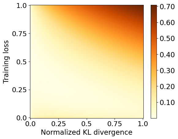
(a) Sub-Bernoulli discrepancy, 168

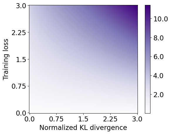
(b) Sub-gamma, 52

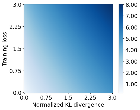
(c) Sub-Laplacian, 56

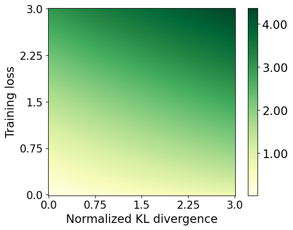
(d) Sub-Poissonian, 45

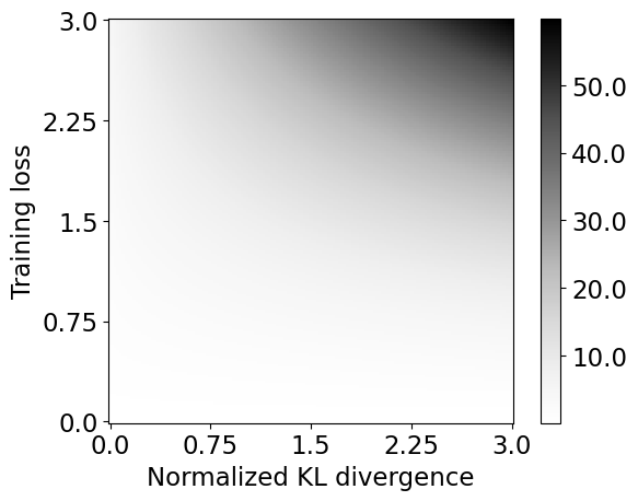
(e) Sub-inverse Gaussian, 162

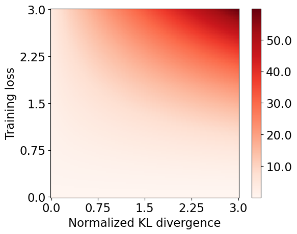
(f) Sub-negative binomial, 165

Figure 2: In Fig. 2(a), we plot 168. In Figs. 2(b) to 2(f), we illustrate the numerical values of the Cramér bounds.

Next, in Figs. 2(b) to 2(f), we evaluate our average Cramér bounds for sub-gamma, sub-Laplacian, sub-Poissonian, sub-inverse Gaussian, and sub-negative binomial losses. Specifically, we present the bound based on 52 with $k=5$ in Fig. 2(b); the bound based on 56 with $b=1$ in Fig. 2(c); the bound based on 45 in Fig. 2(d); the bound based on 162 with $\lambda=1$ in Fig. 2(e); and the bound based on 165 with $r=3$ in Fig. 2(f).

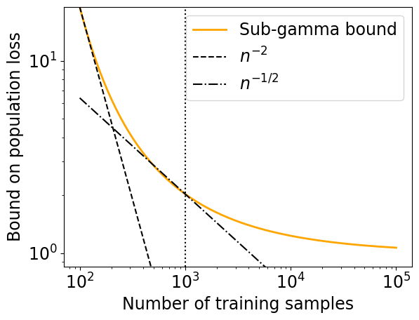
(a) Sub-gamma, $\alpha=1$ 45

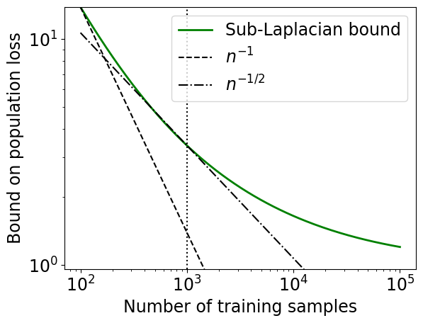
(b) Sub-Laplacian, $\alpha=1$ 162

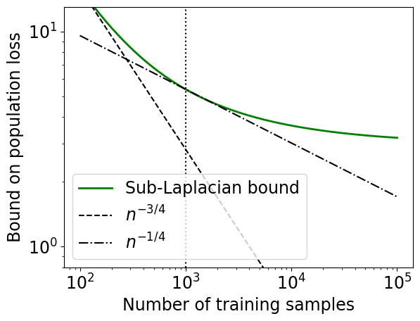
(c) Sub-Laplacian, $\alpha=3$ 165

Figure 3: The $n$-dependence of the the Cramér bounds for sub-gamma and sub-Laplacian losses.

Finally, in Fig. 3, we numerically study the $n$-dependence of the average bounds in terms of the Cramér function for sub-gamma losses, i.e., 52, and for sub-Laplacian losses, i.e., 56. Note that, for the purposes of this evaluation, we assume that the training loss $\alpha$ and KL divergence $\beta$ are fixed, and only the number of samples $n$ varies. This is not a realistic assumption in many settings, as both the training loss and KL divergence will typically depend on the sample size—in particular, the KL divergence tends to increase with $n$. However, this still sheds some light on the behavior of the bounds, and if one knows the dependence of the KL divergence on $n$, this can be incorporated by suitably rescaling.

In Fig. 3(a), we evaluate 52 with $k=5$, training loss $\alpha=1$, and KL divergence $\beta=10^{3}$. For the sub-gamma bound, we find a behavior that is consistent across various values of the training loss: initially, the bound decays as $1/n^{2}$, and when it reaches $n\approx\beta$, it decays as $1/\sqrt{n}$, after which it further slows. This demonstrates that, when the number of samples is low ($n\ll\beta$), the bound rapidly improves as more samples are used, while for larger sample sizes ($n\gg\beta$), the improvement is less pronounced. As a specific example: as $n$ grows from $10^{2}$ to $10^{3}$, the bound decreases by $89\%$, whereas when $n$ grows from $10^{4}$ to $10^{5}$, the bound decreases by $13\%$.

In Fig. 3(b), we evaluate 56 with $b=1$, training loss $\alpha=1$, and KL divergence $\beta=10^{3}$, whereas in Fig. 3(c), we set the training loss to $\alpha=3$. For the sub-Laplacian bound, the picture is less clear. For $\alpha=1$, the bound initially decays as $1/n$, while approximating a $1/\sqrt{n}$ asymptote for $n\approx\beta$ (as for the sub-gamma loss). However, for $\alpha=3$, the initial decay is closer to $n^{-3/4}$, and for $n\approx\beta$, it is approximately $n^{-1/4}$.

References

• Alquier, (2021) Alquier, P. (2021). User-friendly introduction to PAC-Bayes bounds. doi: 10.48550/arxiv.2110.11216. arXiv.
• Alquier and Guedj, (2018) Alquier, P. and Guedj, B. (2018). Simpler PAC-Bayesian bounds for hostile data. Machine Learning, 107(5):887–902.
• Ambroladze et al., (2006) Ambroladze, A., Parrado-Hernandez, E., and Shawe-Taylor, J. (2006). Tighter PAC-Bayes bounds. In Proc. Conf. Neural Inf. Process. Syst. (NeurIPS), Vancouver, Canada.
• Audibert, (2004) Audibert, J.-Y. (2004). A better variance control for PAC-Bayesian classification. Technical report. url: api.semanticscholar.org/CorpusID:18053999.
• Banerjee and Montufar, (2021) Banerjee, P. K. and Montufar, G. (2021). Information complexity and generalization bounds. In Proc. IEEE Int. Symp. Inf. Theory (ISIT), Melbourne, Australia.
• Bégin et al., (2016) Bégin, L., Germain, P., Laviolette, F., and Roy, J.-F. (2016). PAC-Bayesian bounds based on the Rényi divergence. In Proc. Artif. Intell. Statist. (AISTATS), Cadiz, Spain.
• Bernstein, (1929) Bernstein, S. (1929). Sur les fonctions absolument monotones. Acta Mathematica, 52:1–66.
• Biggs and Guedj, (2021) Biggs, F. and Guedj, B. (2021). Differentiable PAC–Bayes objectives with partially aggregated neural networks. Entropy, 23(10).
• Biggs and Guedj, (2022) Biggs, F. and Guedj, B. (2022). Non-vacuous generalisation bounds for shallow neural networks. In Proc. Int. Conf. Mach. Learn. (ICML), Baltimore, MD.
• Boucheron et al., (2013) Boucheron, S., Lugosi, G., and Massart, P. (2013). Concentration inequalities. A nonasymptotic theory of independence. Oxford University Press, Oxford, United Kingdom.
• Bu et al., (2020) Bu, Y., Zou, S., and Veeravalli, V. V. (2020). Tightening mutual information-based bounds on generalization error. IEEE J. Sel. Areas Inf. Theory, 1(1):121–130.
• Catoni, (2007) Catoni, O. (2007). PAC-Bayesian Supervised Classification: The Thermodynamics of Statistical Learning, volume 56. IMS Lecture Notes Monogr. Ser.
• Cover and Thomas, (2006) Cover, T. M. and Thomas, J. A. (2006). Elements of Information Theory (Wiley Series in Telecommunications and Signal Processing). Wiley-Interscience, USA.
• Cramér, (1944) Cramér, H. (1944). On a new limit theorem of the theory of probability. Uspekhi Mathematicheskikh Nauk, (10):166–178.
• Csiszar and Körner, (2011) Csiszar, I. and Körner, J. (2011). Information Theory: Coding Theorems for Discrete Memoryless Systems. Cambridge Univ. Press, Cambridge, U.K., 2nd edition.
• Donsker and Varadhan, (1975) Donsker, M. D. and Varadhan, S. R. S. (1975). Asymptotic evaluation of certain Markov process expectations for large time, i. Comm. Pure Appl. Math, 28(1):1–47.
• Dziugaite et al., (2021) Dziugaite, G. K., Hsu, K., Gharbieh, W., and Roy, D. M. (2021). On the role of data in PAC-Bayes bounds. In Proc. Artif. Intell. Statist. (AISTATS), San Diego, CA, USA.
• Dziugaite and Roy, (2017) Dziugaite, G. K. and Roy, D. M. (2017). Computing nonvacuous generalization bounds for deep (stochastic) neural networks with many more parameters than training data. In Proc. Conf. Uncertainty in Artif. Intell. (UAI), Sydney, Australia.
• Foong et al., (2021) Foong, A. Y. K., Bruinsma, W. P., Burt, D. R., and Turner, R. E. (2021). How tight can PAC-Bayes be in the small data regime? In Proc. Conf. Neural Inf. Process. Syst. (NeurIPS), Virtual Conference.
• Germain et al., (2016) Germain, P., Bach, F., Lacoste, A., and Lacoste-Julien, S. (2016). PAC-Bayesian theory meets Bayesian inference. In Proc. Conf. Neural Inf. Process. Syst. (NeurIPS), Barcelona, Spain.
• Germain et al., (2009) Germain, P., Lacasse, A., Laviolette, F., and Marchand, M. (2009). PAC-Bayesian learning of linear classifiers. In Proc. Int. Conf. Mach. Learning (ICML), Montreal, Canada.
• Grünwald et al., (2023) Grünwald, P., Pérez-Ortiz, M. F., and Mhammedi, Z. (2023). Exponential stochastic inequality. arXiv.
• Guedj, (2019) Guedj, B. (2019). A primer on PAC-Bayesian learning. Proc. 2nd Congress Société Mathématique de France, pages 391–414.
• Haddouche and Guedj, (2023) Haddouche, M. and Guedj, B. (2023). PAC-bayes generalisation bounds for heavy-tailed losses through supermartingales. Transactions on Machine Learning Research (TMLR).
• Haddouche et al., (2021) Haddouche, M., Guedj, B., Rivasplata, O., and Shawe-Taylor, J. (2021). PAC-Bayes unleashed: Generalisation bounds with unbounded losses. Entropy, 23(10).
• Haghifam et al., (2022) Haghifam, M., Moran, S., Roy, D. M., and Dziugiate, G. K. (2022). Understanding generalization via leave-one-out conditional mutual information. In Proc. IEEE Int. Symp. Inf. Theory (ISIT), Espoo, Finland.
• Haghifam et al., (2020) Haghifam, M., Negrea, J., Khisti, A., Roy, D. M., and Dziugaite, G. K. (2020). Sharpened generalization bounds based on conditional mutual information and an application to noisy, iterative algorithms. In Proc. Conf. Neural Inf. Process. Syst. (NeurIPS), Vancouver, Canada.
• Harutyunyan et al., (2021) Harutyunyan, H., Raginsky, M., Steeg, G. V., and Galstyan, A. (2021). Information-theoretic generalization bounds for black-box learning algorithms. In Proc. Conf. Neural Inf. Process. Syst. (NeurIPS), Virtual Conference.
• Hellström and Durisi, (2020) Hellström, F. and Durisi, G. (2020). Generalization bounds via information density and conditional information density. IEEE J. Sel. Areas Inf. Theory, 1(3):824–839.
• Hellström and Durisi, (2022) Hellström, F. and Durisi, G. (2022). A new family of generalization bounds using samplewise evaluated CMI. In Proc. Conf. Neural Inf. Process. Syst. (NeurIPS), New Orleans, LA, USA.
• Hellström et al., (2023) Hellström, F., Durisi, G., Guedj, B., and Raginsky, M. (2023). Generalization bounds: Perspectives from information theory and PAC-Bayes. doi: 10.48550/arxiv.2309.04381. arXiv.
• Kullback, (1954) Kullback, S. (1954). Certain inequalities in information theory and the Cramér-Rao inequality. The Annals of Mathematical Statistics, 25(4):745 – 751.
• Langford and Caruana, (2001) Langford, J. and Caruana, R. (2001). (not) bounding the true error. In Proc. Conf. Neural Inf. Process. Syst. (NeurIPS), Vancouver, Canada.
• Langford and Seeger, (2001) Langford, J. and Seeger, M. (2001). Bounds for averaging classifiers. CMU Technical report, CMU-CS-01-102.
• Letarte et al., (2019) Letarte, G., Germain, P., Guedj, B., and Laviolette, F. (2019). Dichotomize and generalize: PAC-Bayesian binary activated deep neural networks. In Proc. Conf. Neural Inf. Process. Syst. (NeurIPS), Vancouver, Canada.
• Lotfi et al., (2022) Lotfi, S., Finzi, M., Kapoor, S., Potapczynski, A., Goldblum, M., and Wilson, A. G. (2022). PAC-Bayes compression bounds so tight that they can explain generalization. In Proc. Conf. Neural Inf. Process. Syst. (NeurIPS), New Orleans, LA, USA.
• Lugosi and Neu, (2023) Lugosi, G. and Neu, G. (2023). Online-to-PAC conversions: Generalization bounds via regret analysis. arXiv.
• Maurer, (2004) Maurer, A. (2004). A note on the PAC Bayesian theorem. doi: 10.48550/arxiv.cs/0411099. arXiv.
• McAllester, (1998) McAllester, D. A. (1998). Some PAC-Bayesian theorems. In Proc. Conf. Learn. Theory (COLT), Madison, WI, USA.
• McAllester, (2003) McAllester, D. A. (2003). PAC-Bayesian stochastic model selection. Mach. Learn., 51:5–21.
• Mhammedi et al., (2020) Mhammedi, Z., Guedj, B., and Williamson, R. C. (2020). PAC-Bayesian bound for the conditional value at risk. In Proc. Conf. Neural Inf. Process. Syst. (NeurIPS), volume 33.
• Negrea et al., (2019) Negrea, J., Haghifam, M., Dziugaite, G. K., Khisti, A., and Roy, D. M. (2019). Information-theoretic generalization bounds for SGLD via data-dependent estimates. In Proc. Conf. Neural Inf. Process. Syst. (NeurIPS), Vancouver, Canada.
• Neyshabur et al., (2018) Neyshabur, B., Bhojanapalli, S., and Srebro, N. (2018). A PAC-Bayesian approach to spectrally-normalized margin bounds for neural networks. In Proc. Int. Conf. Learn. Representations (ICLR), Vancouver, Canada.
• Nielsen and Garcia, (2009) Nielsen, F. and Garcia, V. (2009). Statistical exponential families: a digest with flash cards. doi: 10.48550/arXiv.0911.4863. arXiv.
• Pérez-Ortiz et al., (2021) Pérez-Ortiz, M., Rivasplata, O., Shawe-Taylor, J., and Szepesvári, C. (2021). Tighter risk certificates for neural networks. Journal of Machine Learning Research (JMLR), 22(227):1–40.
• Rivasplata et al., (2020) Rivasplata, O., Kuzborskij, I., Szepesvari, C., and Shawe-Taylor, J. (2020). PAC-Bayes analysis beyond the usual bounds. In Proc. Conf. Neural Inf. Process. Syst. (NeurIPS), Vancouver, Canada.
• Rockafellar, (1970) Rockafellar, R. T. (1970). Convex analysis. Princeton Mathematical Series. Princeton University Press, Princeton, N. J., USA.
• Rodríguez-Gálvez et al., (2020) Rodríguez-Gálvez, B., Bassi, G., Thobaben, R., and Skoglund, M. (2020). On random subset generalization error bounds and the stochastic gradient langevin dynamics algorithm. In Proc. IEEE Inf. Theory Workshop (ITW), Riva del Garda, Italy.
• Rodríguez-Gálvez et al., (2023) Rodríguez-Gálvez, B., Thobaben, R., and Skoglund, M. (2023). More PAC-Bayes bounds: From bounded losses, to losses with general tail behaviors, to anytime-validity. In Workshop on PAC-Bayes Meets Interactive Learning (PBMIL), Honolulu, HI, USA.
• Russo and Zou, (2016) Russo, D. and Zou, J. (2016). Controlling bias in adaptive data analysis using information theory. In Proc. Artif. Intell. Statist. (AISTATS), Cadiz, Spain.
• Seldin et al., (2012) Seldin, Y., Laviolette, F., Cesa-Bianchi, N., Shawe-Taylor, J., and Auer, P. (2012). PAC-Bayesian inequalities for Martingales. IEEE Trans. Inf. Theory, 58(12):7086–7093.
• Shawe-Taylor and Williamson, (1997) Shawe-Taylor, J. and Williamson, R. C. (1997). A PAC analysis of a Bayesian estimator. In Proc. Conf. Learn. Theory (COLT).
• Steinke and Zakynthinou, (2020) Steinke, T. and Zakynthinou, L. (2020). Reasoning about generalization via conditional mutual information. In Proc. Conf. Learn. Theory (COLT), Graz, Austria.
• Wainwright, (2019) Wainwright, M. J. (2019). High-Dimensional Statistics: a Non-Asymptotic Viewpoint. Cambridge Univ. Press, Cambridge, U.K.
• Wang and Mao, (2023) Wang, Z. and Mao, Y. (2023). Tighter Information-Theoretic Generalization Bounds from Supersamples. In Proc. Int. Conf. Mach. Learning (ICML), Honolulu, HI, USA.
• Wasserman, (2010) Wasserman, L. (2010). All of statistics : a concise course in statistical inference. Springer, New York.
• Wu et al., (2023) Wu, X., Manton, J. H., Aickelin, U., and Zhu, J. (2023). On the tightness of information-theoretic bounds on generalization error of learning algorithms. arXiv. doi: 10.48550/arxiv.2303.14658.
• Xu and Raginsky, (2017) Xu, A. and Raginsky, M. (2017). Information-theoretic analysis of generalization capability of learning algorithms. In Proc. Conf. Neural Inf. Process. Syst. (NeurIPS), Long Beach, CA, USA.
• Zhang, (2006) Zhang, T. (2006). Information-theoretic upper and lower bounds for statistical estimation. IEEE Trans. Inf. Theory, 52(4):1307–1321.
• Zhang et al., (2007) Zhang, Z., Sun, H., and Zhong, F. (2007). Information geometry of the power inverse Gaussian distribution. APPS. Applied Sciences, 9:194–203.
• Zhou et al., (2019) Zhou, W., Veitch, V., Austern, M., Adams, R., and Orbanz, P. (2019). Non-vacuous generalization bounds at the ImageNet scale: a PAC-Bayesian compression approach. In Proc. Int. Conf. Learn. Representations (ICLR), New Orleans, LA.