Label-efficient Segmentation via Affinity Propagation

Abstract

Weakly-supervised segmentation with label-efficient sparse annotations has attracted increasing research attention to reduce the cost of laborious pixel-wise labeling process, while the pairwise affinity modeling techniques play an essential role in this task. Most of the existing approaches focus on using the local appearance kernel to model the neighboring pairwise potentials. However, such a local operation fails to capture the long-range dependencies and ignores the topology of objects. In this work, we formulate the affinity modeling as an affinity propagation process, and propose a local and a global pairwise affinity terms to generate accurate soft pseudo labels. An efficient algorithm is also developed to reduce significantly the computational cost. The proposed approach can be conveniently plugged into existing segmentation networks. Experiments on three typical label-efficient segmentation tasks, i.e. box-supervised instance segmentation, point/scribble-supervised semantic segmentation and CLIP-guided semantic segmentation, demonstrate the superior performance of the proposed approach.

1 Introduction

Segmentation is a widely studied problem in computer vision, aiming at generating a mask prediction for a given image, e.g., grouping each pixel to an object instance (instance segmentation) or assigning each pixel a category label (semantic segmentation). While having achieved promising performance, most of the existing approaches are trained in a fully supervised manner, which heavily depend on the pixel-wise mask annotations, incurring tedious labeling costs [1]. Weakly-supervised methods have been proposed to reduce the dependency on dense pixel-wise labels with label-efficient sparse annotations, such as points [2, 3, 4], scribbles [5, 6, 7], bounding boxes [8, 9, 10, 11] and image-level labels [12, 13, 14, 15]. Such methods make dense segmentation more accessible with less annotation costs for new categories or scene types.

Most of the existing weakly-supervised segmentation methods [16, 13, 8, 17, 3, 10] adopt the local appearance kernel to model the neighboring pairwise affinities, where spatially nearby pixels with similar color (i.g., LAB color space [8, 3] or RGB color space [13, 16, 17, 10]) are likely to be in the same class. Though having proved to be effective, these methods suffer from two main limitations. First, the local operation cannot capture global context cues and capture long-range affinity dependencies. Second, the appearance kernel fails to take the intrinsic topology of objects into account, and lacks capability of detail preservation.

To address the first issue, one can directly enlarge the kernel size to obtain a large receptive filed. However, this will make the segmentation model insensitive to local details and increase the computational cost greatly. Some methods [14, 12] model the long-range affinity via random walk [18], but they cannot model the fine-grained semantic affinities. As for the second issue, the tree-based approaches [7, 19] are able to preserve the geometric structures of objects, and employ the minimum spanning tree [20] to capture the pairwise relationship. However, the affinity interactions with distant nodes will decay rapidly as the distance increases along the spanning tree, which still focuses on the local nearby regions. LTF-V2 [21] enables the long-range tree-based interactions but it fails to model the valid pairwise affinities for label-efficient segmentation task.

With the above considerations, we propose a novel component, named Affinity Propagation (APro), which can be easily embedded in existing methods for label-efficient segmentation. Firstly, we define the weakly-supervised segmentation from a new perspective, and formulate it as a uniform affinity propagation process. The modelled pairwise term propagates the unary term to other nearby and distant pixels and updates the soft pseudo labels progressively. Then, we introduce the global affinity propagation, which leverages the topology-aware tree-based graph and relaxes the geometric constraints of spanning tree to capture the long-range pairwise affinity. With the efficient design, the $\mathcal{O}(N^{2})$ complexity of brute force implementation is reduced to $\mathcal{O}(N\log N)$, and the global propagation approach can be performed with much less resource consumption for practical applications. Although the long-range pairwise affinity is captured, it inevitably brings in noises based on numerous pixels in a global view. To this end, we introduce a local affinity propagation to encourage the piece-wise smoothness with spatial consistency. The formulated APro can be embedded into the existing segmentation networks to generate accurate soft pseudo labels online for unlabeled regions. As shown in Fig. 1, it can be seamlessly plugged into the existing segmentation networks for various tasks to achieve weakly-supervised segmentation with label-efficient sparse annotations.

We perform experiments on three typical label-efficient segmentation tasks, i.e. box-supervised instance segmentation, point/scribble-supervised semantic segmentation and annotation-free semantic segmentation with pretrained CLIP model, and the results demonstrated the superior performance of our proposed universal label-efficient approach.

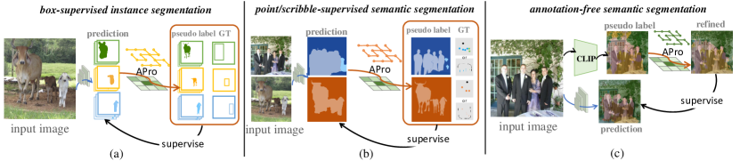
Figure 1: The proposed approach upon the typical weakly-supervised segmentation tasks with label-efficient annotations, including (a) box-supervised instance segmentation, (b) point/scribble-supervised semantic segmentation and (c) annotation-free semantic segmentation with CLIP pretrained model.

2 Related Work

Label-efficient Segmentation. Label-efficient segmentation, which is based on the weak supervision from partial or sparse labels, has been widely explored [1]. Different from semi-supervised settings [22, 23], this paper mainly focuses on the segmentation with sparse labels. In earlier literature [24, 25, 26, 27, 28], it primarily pertained to image-level labels. Recently, diverse sparse annotations have been employed, including point, scribble, bounding box , image-level label and the combinations of them. We briefly review the weakly-supervised instance segmentation, semantic segmentation and panoptic segmentation tasks in the following.

For weakly-supervised instance segmentation, box-supervised methods [16, 8, 17, 9, 29, 30, 11, 10, 31] are dominant and perform on par with fully-supervised segmentation approaches. Besides, the “points + bounding box” annotation can also achieve competitive performance [32, 33]. As for weakly-supervised semantic segmentation, previous works mainly focus on the point-level supervision [2, 34, 6] and scribble-level supervision [5, 35, 36], which utilize the spatial and color information of the input image and are trained with two stages. Liang et al. [7] introduced an effective tree energy loss based on the low-level and high-level features for point/scribble/block-supervised semantic segmentation. For semantic segmentation, the supervision of image-level labels has been well explored [12, 37, 15, 14]. Recently, some works have been proposed to make use of the large-scale pretrained CLIP model [38] to achieve weakly-supervised or annotation-free semantic segmentation [39, 40]. In addition, weakly-supervised panoptic segmentation methods [3, 41, 4] with a single and multiple points annotation have been proposed. In this paper, we aim to develop a universal component for various segmentation tasks, which can be easily plugged into the existing segmentation networks.

Pairwise Affinity Modeling. Pairwise affinity modeling plays an important role in many computer vision tasks. Classical methods, like CRF [42], make full use of the color and spatial information to model the pairwise relations in the semantic labeling space. Some works use it as a post-processing module [43], while others integrate it as a jointly-trained part into the deep neural network [44, 45]. Inspired by CRF, some recent approaches explore the local appearance kernel to tap the neighboring pairwise affinities, where spatially nearby pixels with similar colors are more likely to fall into the same class. Tian et al. [8] proposed the local pairwise loss, which models the neighboring relationship in LAB color space. Some works [10, 16, 17] focus on the pixel relation in RGB color space directly, and achieve competitive performance. However, the local operation fails to capture global context cues and lacks the long-range affinity dependencies. Furthermore, the appearance kernel cannot reflect the topology of objects, missing the details of semantic objects. To model the structural pair-wise relationship, tree-based approaches [7, 19] leverage the minimum spanning tree [20] to capture the topology of objects in the image. However, the affinity interactions with distant nodes decay rapidly as the distance increases along the spanning tree. Besides, Zhang et al. [35] proposed an affinity network to convert an image to a weighted graph, and model the node affinities by the graph neural network (GNN). Different from these methods, in this work we model the pairwise affinity from a new affinity propagation perspective both globally and locally.

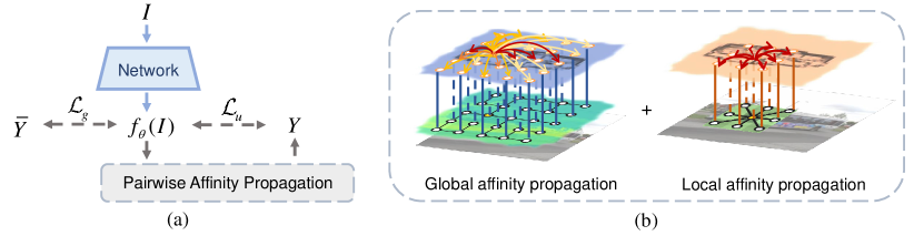
Figure 2: Overview of our APro approach. (a) The general weakly supervised segmentation framework with the proposed pairwise affinity propagation. (b) The proposed approach consists of global affinity propagation (GP) and local affinity propagation (LP) to generate accurate pseudo labels.

3 Methodology

In this section, we introduce our proposed affinity propagation (APro) approach to label-efficient segmentation. First, we define the problem and model the APro framework in Section 3.1. Then, we describe the detailed pairwise affinity propagation method in Section 3.2. Finally, we provide an efficient implementation of our method in Section 3.3.

3.1 Problem Definition and Modeling

Given an input image $I=\{x_{i}\}^{N}$ with $N$ pixels and its available sparse ground truth labeling ${\bar{Y}}$ (i.e. points, scribble, or bounding box), and let ${f_{\theta}}(I)$ be the output of a segmentation network with the learnable parameters $\theta$, the whole segmentation network can be regarded as a neural network optimization problem as follows:

$$\mathop{\min}\limits_{\theta}\left\{{\mathcal{L}_{g}({f_{\theta}}(I),{\bar{Y}})+\mathcal{L}_{u}({f_{\theta}}(I),Y)}\right\},$$ (1)

where $\mathcal{L}_{g}$ is a ground truth loss on the set of labeled pixels $\Omega_{g}$ with ${\bar{Y}}$ and $\mathcal{L}_{u}$ is a loss on the unlabeled regions $\Omega_{u}$ with the pseudo label $Y$. As shown in Fig. 2-(a), our goal is to obtain the accurate pseudo label $Y$ by leveraging the image pixel affinities for unlabeled regions.

As in the classic MRF/CRF model [46, 42], the unary term reflects the per-pixel confidence of assigning labels, while pairwise term captures the inter-pixel constraints. We define the generation of pseudo label $Y$ as an affinity propagation process, which can be formulated as follows:

$${y_{i}}=\frac{1}{{{z_{i}}}}\sum\limits_{{j}\in\tau}{\phi({x_{j}})}\psi({x_{i}},{x_{j}}),$$ (2)

where ${\phi}({x_{j}})$ denotes the unary potential term, which is used to align $y_{j}$ and the corresponding network prediction based on the available sparse labels. $\psi({x_{i}},{x_{j}})$ indicates the pairwise potential, which models the inter-pixel relationships to constrain the predictions and produce accurate pseudo labels. $\tau$ is the region with different receptive fields. $z_{i}$ is the summation of pairwise affinity $\psi({x_{i}},{x_{j}})$ along with $j$ to normalize the response.

Notably, we unify both global and local pairwise potentials in an affinity propagation process formulated in Eq. 2. As shown in Fig. 2-(b), the global affinity propagation (GP) can capture the pairwise affinities with topological consistency in a global view, while the local affinity propagation (LP) can obtain the pairwise affinities with local spatial consistency. Through the proposed component, the soft pseudo labels $Y$ can be obtained. We assign each $y_{i}$ from GP and LP with the network prediction $p_{i}$ and directly employ the distance measurement function as the objective for unlabeled regions $\Omega_{u}$. Simple $L_{1}$ distance is empirically adopted in our implementation.

3.2 Pairwise Affinity Propagation

3.2.1 Global Affinity Propagation

We firstly provide a solution to model the global affinity efficiently based on the input image. Specifically, we represent an input image as a 4-connected planar graph $\mathcal{G}$, where each node is adjacent to up to 4 neighbors. The weight of the edge measures the image pixel distance between adjacent nodes. Inspired by tree-based approaches [47, 19], we employ the minimum spanning tree (MST) algorithm [20] to remove the edge with a large distance to obtain the tree-based sparse graph $\mathcal{G}_{T}$, i.e., $\mathcal{G}_{T}\leftarrow\text{MST}(\mathcal{G})$ and $\mathcal{G}_{T}=\{\mathcal{V},\mathcal{E}\}$, where $\mathcal{V}=\{\mathcal{V}_{i}\}^{N}$ is the set of nodes and $\mathcal{E}=\{\mathcal{E}_{i}\}^{N-1}$ denotes the set of edges.

Then, we model the global pairwise potential by iterating over each node. To be specific, we take the current node as the root of the spanning tree $\mathcal{G}_{T}$ and propagate the long-range affinities to other nodes. While the distant nodes along the spanning tree need to pass through nearby nodes along the path of spanning tree, the distance-insensitive max affinity function can alleviate this geometric constraint and relax the affinity decay for long-range nodes. Hence, we define the global pairwise potential $\psi_{g}$ as follows:

$${\psi_{g}}({x_{i}},{x_{j}})=\mathop{\mathcal{T}({I_{i}},{I_{j}})}\limits_{\forall j\in\mathcal{V}}=\exp(-\mathop{\max}\limits_{\forall(k,l)\in{\mathbb{E}_{i,j}}}\frac{{{w_{k,l}}}}{{{\zeta_{g}}^{2}}}),$$ (3)

where $\mathcal{T}$ denotes the global tree. $\mathbb{E}_{i,j}$ is the set of edges in the path of $\mathcal{T}$ from node $j$ to node $i$. $w_{k,l}$ indicates the edge weight between the adjacent nodes $k$ and $l$, which is represented as the Euclidean distance between pixel values of two adjacent nodes, $\textit{i.e.},{w_{k,l}}={\left|{{I_{k}}-{I_{l}}}\right|^{2}}$. $\zeta_{g}$ controls the degree of similarity with the long-range pixels. In this way, the global affinity propagation (GP) process to obtain the soft label $y^{g}$ can be formulated as follows:

$$y_{i}^{g}=\frac{1}{{{z_{i}^{g}}}}\sum\limits_{j\in\mathcal{V}}{\phi({x_{j}})}{\psi_{g}}({x_{i}},{x_{j}}),\ \ {z_{i}^{g}}=\sum\limits_{j\in{\mathcal{V}}}{{\psi_{g}}({x_{i}},{x_{j}})},$$ (4)

where interactions with distant nodes are performed over tree-based topology. In addition to utilizing low-level image, we empirically employ high-level feature as input to propagate semantic affinity.

3.2.2 Local Affinity Propagation

The long-range pairwise affinity is inevitably noisy since it is computed based on the susceptible image features in a global view. The spatially nearby pixels are more likely to have the same label, while they have certain difference in color and intensity, etc. Hence, we further introduce the local affinity propagation (LP) to promote the piece-wise smoothness. The Gaussian kernel is widely used to capture the local relationship among the neighbouring pixels in previous works [45, 8, 10]. Different from these works, we define the local pairwise affinity via the formulated affinity propagation process. The local pairwise term $\psi_{s}$ is defined as:

$${\psi_{s}}({x_{i}},{x_{j}})=\mathop{{\cal K}{\rm{}}({I_{i}},{I_{j}})}\limits_{j\in{{\cal N}}(i)}=\exp\left({\frac{{-{{\left|{{I_{i}}-{I_{j}}}\right|}^{2}}}}{{\zeta_{s}^{2}}}}\right),$$ (5)

where ${\cal K}$ denotes the Gaussian kernel, $\mathcal{N}(i)$ is the set containing all local neighbor pixels. The degree of similarity is controlled by parameter $\zeta_{s}$. Then the pseudo label $y^{s}$ can be obtained via the following affinity propagation:

$${y^{s}_{i}}=\frac{1}{{{{z}_{i}^{s}}}}\sum\limits_{j\in{\mathcal{N}}(i)}{{\phi}({x_{j}})}{\psi_{s}}({x_{i}},{x_{j}}),\ \ {z_{i}^{s}}=\sum\limits_{j\in{\mathcal{N}}(i)}{{\psi_{s}}({x_{i}},{x_{j}})},$$ (6)

where the local spatial consistency is maintained based on high-contrast neighbors. To obtain a robust segmentation performance, multiple iterations are required. Notably, our LP process ensures a fast convergence, which is 5$\times$ faster than MeanField-based method [10, 42]. The details can be found in the experimental section 4.4.

3.3 Efficient Implementation

Given a tree-based graph $\mathcal{G}_{T}=\{\mathcal{V},\mathcal{E}\}$ in the GP process, we define the maximum $\bm{w}$ value of the path through any two vertices as the transmission cost $\mathcal{C}$. One straightforward approach to get $y_{i}^{g}$ of vertex $i$ is to traverse each vertex $j$ by Depth First Search or Breadth First Search to get the transmission cost $\mathcal{C}_{i,j}$ accordingly. Consequently, the computational complexity required to acquire the entire output ${y^{g}}$ is $\mathcal{O}(N^{2})$, making it prohibitive in real-world applications.

Instead of calculating and updating the transmission cost of any two vertices, we design a lazy update algorithm to accelerate the GP process. Initially, each node is treated as a distinct union, represented by $\mathcal{U}$. Unions are subsequently connected based on each edge $w_{k,l}$ in ascending order of $\bm{w}$. We show that when connecting two unions $\mathcal{U}_{k}$ and $\mathcal{U}_{l}$, $w_{k,l}$ is equivalent to the transmission cost for all nodes within $\mathcal{U}_{k}$ and $\mathcal{U}_{l}$. This is proved in the supplementary material.

To efficiently update values, we introduce a Lazy Propagation scheme. We only update the value of the root node and postpone the update of its descendants. The update information is retained in a lazy tag $\mathcal{Z}$ and is updated as follows:

$$\mathcal{Z}(\delta)_{k^{*}}=\mathcal{Z}(\delta)_{k^{*}}+\begin{cases}\text{exp}(-w_{k,l}/{\zeta_{g}}^{2})S(\delta)_{l}&\mathcal{U}_{k}.\text{rank}>\mathcal{U}_{l}.\text{rank},\\ \text{exp}(-w_{k,l}/{\zeta_{g}}^{2})S(\delta)_{l}-\mathcal{Z}(\delta)_{l^{*}}&\text{otherwise},\end{cases}$$ (7)

where $S(\delta)_{i}=\sum_{j\in\mathcal{U}_{i}}\delta_{j}$, $\delta$ means different inputs, including the dense prediction $\phi(x)$ and all-one matrix $\Lambda$. $k^{*}/l^{*}$ denotes the root node of node $k/l$.

Once all unions are connected, the lazy tags can be propagated downward from the root node to its descendants. For the descendants, the global affinity propagation term is presented as follows:

$$LProp(\delta)_{i}=\delta_{i}+\sum_{r\in Asc_{\mathcal{G}_{T}}(i)\cup\{i\}}\mathcal{Z}(\delta)_{r},$$ (8)

where $Asc_{\mathcal{G}_{T}}(i)$ represents the ascendants of node $i$ in the tree $\mathcal{G}_{T}$. As shown in Algorithm 1, the disjoint-set data structure is employed to implement the proposed algorithm. In our implementation, a Path Compression strategy is applied, connecting each node on the path directly to the root node. Consequently, it is sufficient to consider the node itself and its parent node to obtain $LProp$.

Input: Tree $\mathcal{G}_{T}\in\mathbb{N}^{e\times 2}$; Pairwise distance $\bm{w}\in\mathbb{R}^{N}$; Dense predictions $\phi(x)\in\mathbb{R}^{N}$;

         Vertex num $N$; Edge num $e=N-1$; Set of vertices $\mathcal{V}$.

Output: $y^{g}\in\mathbb{R}^{N}$.

$\Lambda\,\leftarrow\bm{1}\in\mathbb{R}^{N}$

$F\leftarrow\{0,1,2,...,N-1\}$ $\triangleright$ Initialize each vertex as a connected block

Sort {$\mathcal{G}_{T}$, $\bm{w}$} in ascending order of $\bm{w}$. $\triangleright$ Quick Sort

for $(k,l)\in\mathcal{G}_{T},w_{i}\in\bm{w}$  do

       $a$ $\leftarrow$ find($k$), $b$ $\leftarrow$ find($l$) $\triangleright$ Find the root node with Path Compression

       Update{$\mathcal{Z}(\phi)_{a}$, $\mathcal{Z}(\Lambda)_{a}$, $\mathcal{Z}(\phi)_{b}$, $\mathcal{Z}(\Lambda)_{b}$} $\triangleright$ Add lazy tag

       if $S_{a}<S_{b}$  then

             swap($a,b$) $\triangleright$ Merge by Rank

            

      $F_{b}$ $\leftarrow$ $a$ $\triangleright$ Merge two connected blocks

      

for $v\in\mathcal{V}$ do

       $p\leftarrow$ find($v$)

       for $\delta\in\{\phi,\Lambda\}$ do

             if $p=v$ then

                   $LProp(\delta)_{v}=\mathcal{Z}(\delta)_{v}+\delta_{v}$

                  

            else

                   $LProp(\delta)_{v}=\mathcal{Z}(\delta)_{p}+\mathcal{Z}(\delta)_{v}+\delta_{v}$

                  

            

      $y_{v}^{g}=\frac{LProp(\phi)_{v}}{LProp(\Lambda)_{v}}$ $\triangleright$ Normalization

      

return $y^{g}$

Algorithm 1 Algorithm for GP process

Time complexity. For each channel of the input, the average time complexity of sorting is $\mathcal{O}(N\log N)$. In the merge step, we utilize the Path Compression and Union-by-Rank strategies, which have a complexity of $\mathcal{O}(\alpha(N))$[48]. After merging all the concatenated blocks, the lazy tags can be propagated in $\mathcal{O}(N)$ time. Hence, the overall complexity is $\mathcal{O}(N\log N)$. Note that the batches and channels are independent of each other. Thus, the algorithm can be executed in parallel for both batches and channels for practical implementations. As a result, the proposed algorithm reduces the computational complexity dramatically.

4 Experiments

4.1 Weakly-supervised Instance Segmentation

Datasets. As in prior arts [8, 9, 16, 17], we conduct experiments on two widely used datasets for the weakly box-supervised instance segmentation task:

• COCO [49], which has 80 classes with 115K train2017 images and 5K val2017 images.

• Pascal VOC [43] augmented by SBD [50] based on the original Pascal VOC 2012 [51], which has 20 classes with 10,582 trainaug images and 1,449 val images.

Base Architectures and Competing Methods. In the evaluation, we apply our proposed APro to two representative instance segmentation architectures, SOLOv2 [52] and Mask2Former [53], with different backbones (i.e., ResNet [54], Swin-Transformer [55]) following Box2Mask  [11]. We compare our approach with its counterparts that model the pairwise affinity based on the image pixels without modifying the base segmentation network for box-supervised setting. Specifically, the compared methods include Pairwise Loss [8], TreeEnergy Loss [7] and CRF Loss [10]. For fairness, we re-implement these models using the default setting in MMDetection [56].

Implementation Details. We follow the commonly used training settings on each dataset as in MMDetection [56]. All models are initialized with ImageNet [57] pretrained backbone. For SOLOv2 framework [52], the scale jitter is used, where the shorter image side is randomly sampled from 640 to 800 pixels. For Mask2Former framework [53], the large-scale jittering augmentation scheme [58] is employed with a random scale sampled within range [0.1, 2.0], followed by a fixed size crop to 1024×1024. The initial learning rate is set to 10^-4 and the weight decay is 0.05 with 16 images per mini-batch. The box projection loss [8, 9] is employed to constrain the network prediction within the bounding box label as the unary term $\phi$. COCO-style mask AP (%) is adopted for evaluation.

Quantitative Results. Table 1 shows the quantitative results. We compare the approaches with the same architecture for fair comparison. The state-of-the-art methods are listed for reference. One can see that our APro method outperforms its counterparts across Pascal VOC and COCO datasets.

• Pascal VOC [43] val. Under the SOLOv2 framework, our approach achieves 37.1% AP and 38.4% AP with 12 epochs and 36 epochs, respectively, outperforming other methods by 1.4%-2.5% mask AP with ResNet-50. With the Mask2Former framework, our approach also outperforms its counterparts. Furthermore, with the Swin-L backbone [55], our proposed approach achieves very promising performance, 49.6% mask AP with 50 epochs.

• COCO [49] val. Under the SOLOv2 framework, our approach achieves 32.0% AP and 32.9% AP with 12 epochs and 36 epochs, and surpasses its best counterpart by 1.0% AP and 0.4% AP using ResNet-50, respectively. Under the Mask2Former framework, our method still achieves the best performance with ResNet-50 backbone. Furthermore, equipped with stronger backbones, our approach obtains more robust performance, achieving 38.0% mask AP with ResNet-101, and 41.0% mask AP using Swin-L backbone.

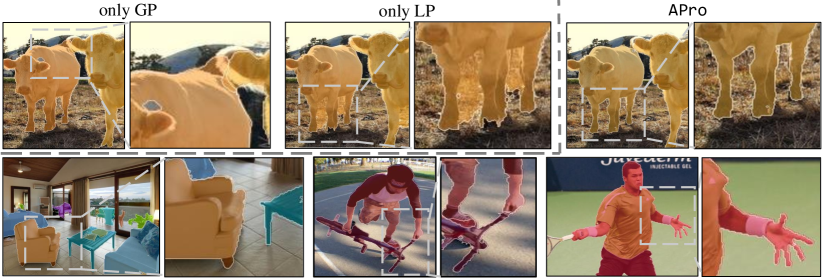
Figure 4: Qualitative results with different pairwise affinity terms on weakly supervised instance segmentation. Our method only with GP process preserves details without local consistency, while the model with only LP process encourages the local smoothness without topology-wise details. Our APro approach yields high-quality predictions with fine-grained details.

Qualitative Results. Fig. 3 illustrates the visual comparisons on affinity maps of our APro and other approaches, and Fig. 4 compares the segmentation results. One can clearly see that our method captures accurate pairwise affinity with object’s topology and yields more fine-grained predictions.

Table 1: Quantitative results (§4.1) on Pascal VOC [43] and COCO  val [49] with mask AP(%).

			Pascal VOC			COCO
Method	Backbone	#Epoch	AP	AP${}_{\text{50}}$	AP${}_{\text{75}}$	AP	AP${}_{\text{50}}$	AP${}_{\text{75}}$
BBTP [NeurIPS19] [16]	ResNet-101	12	23.1	54.1	17.1	21.1	45.5	17.2
1-9[1pt/1pt] BoxInst [CVPR21] [8]	ResNet-50	36	34.3	58.6	34.6	31.8	54.4	32.5
DiscoBox [ICCV21] [17]	ResNet-50	36	-	59.8	35.5	31.4	52.6	32.2
BoxLevelset [ECCV22] [9]	ResNet-50	36	36.3	64.2	35.9	31.4	53.7	31.8
SOLOv2 Framework
Pairwise Loss [CVPR21] [8]	ResNet-50	12	35.7	64.3	35.1	31.0	52.8	31.5
TreeEnergy Loss [CVPR22] [7]	ResNet-50	12	35.0	64.4	34.7	30.9	52.9	31.3
CRF Loss [CVPR23] [10]	ResNet-50	12	35.0	64.7	34.9	30.9	53.1	31.4
APro(Ours)	ResNet-50	12	37.1	65.1	37.0	32.0	53.4	32.9
1-9[1pt/1pt] Pairwise Loss [CVPR21] [8]	ResNet-50	36	36.5	63.4	38.1	32.4	54.5	33.4
TreeEnergy Loss [CVPR22] [7]	ResNet-50	36	36.1	63.5	36.1	31.4	54.0	31.2
CRF Loss [CVPR23] [10]	ResNet-50	36	35.9	64.0	35.7	32.5	54.9	33.2
APro(Ours)	ResNet-50	36	38.4	65.4	39.8	32.9	55.2	33.6
APro(Ours)	ResNet-101	36	40.5	67.9	42.6	34.3	57.0	35.3
Mask2Former Framework
Pairwise Loss [CVPR21] [8]	ResNet-50	12	35.2	62.9	33.9	33.8	57.1	34.0
TreeEnergy Loss [CVPR22] [7]	ResNet-50	12	36.0	65.0	34.3	33.5	56.7	33.7
CRF Loss [CVPR23] [10]	ResNet-50	12	35.7	64.3	35.2	33.5	57.5	33.8
APro(Ours)	ResNet-50	12	37.0	65.1	37.0	34.4	57.7	35.3
1-9[1pt/1pt] APro(Ours)	ResNet-50	50	42.3	70.6	44.5	36.1	62.0	36.7
APro(Ours)	ResNet-101	50	43.6	72.0	45.7	38.0	63.6	38.7
APro(Ours)	Swin-L	50	49.6	77.6	53.1	41.0	68.3	41.9

4.2 Weakly-supervised Semantic Segmentation

Datasets. We conduct experiments on the widely-used Pascal VOC2012 dataset [51], which contains 20 object categories and a background class. As in  [6, 7], the augmented Pascal VOC dataset is adopted here. The point [2] and scribble [5] annotations are employed for weakly point-supervised and scribble-supervised settings, respectively.

Table 2: Quantitative results (§4.2) on Pascal VOC2012 [51] val with mean IoU(%).

Method					Backbone	Supervision	CRF Post.	mIoU
†KernelCut Loss [ECCV18] [6]	DeepLabV2		✓	57.0
∗TEL [CVPR22] [7]	LTF		✗	66.8
APro(Ours)	LTF	Point	✗	67.7
†NormCut Loss [CVPR18] [59]	DeepLabV2		✓	74.5
†DenseCRF Loss [ECCV18] [6]	DeepLabV2		✓	75.0
†KernelCut Loss [ECCV18] [6]	DeepLabV2		✓	75.0
†GridCRF Loss [ICCV19] [36]	DeepLabV2		✗	72.8
PSI [ICCV21] [36]	DeepLabV3		✗	74.9
∗TEL [CVPR22] [7]	LTF		✗	76.2
APro(Ours)	LTF	Scribble	✗	76.6
$\dagger$:adopting multi-stage training, $\ast$:our re-implementation.

Implementation Details. As in [7], we adopt LTF [19] as the base segmentation model. The input size is 512 $\times$ 512. The SGD optimizer with momentum of 0.9 and weight decay of 10^-4 is used. The initial learning rate is 0.001, and there are 80k training iterations. The same data augmentations as in [7] are utilized. We employ the partial cross-entropy loss to make full use of the available point/scribble labels and constrain the unary term. ResNet-101 [54] pretrained on ImageNet [57] is adopted as backbone network for all methods.

Quantitative Results. As shown in Table 2, we compare our APro approach with the state-of-the-art methods on point-supervised and scribble-supervised semantic segmentation, respectively.

• Point-wise supervision. With DeepLabV2 [43], KernelCut Loss [6] achieves 57.0% mIoU. Equipped with LTF [19], TEL [7] achieves 66.8% mIoU. Our APro achieves 67.7% mIoU, outperforming the previous best method TEL [7] by 0.9% mIoU.

• Scribble-wise supervision. The scribble-supervised approaches are popular in weakly supervised semantic segmentation. We apply the proposed approach under the single-stage training framework without calling for CRF post-processing during testing. Compared with the state-of-the-art methods, our approach achieves better performance with 76.6% mIoU.

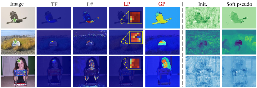
Figure 3: Visual comparisons of pairwise affinity maps based on the RGB image for a specific position (green star), including TreeFilter (TF) [19], local kernels with full image size (L#), and our presented LP and GP processes. The GP process can capture the long-range pairwise affinity with object’s topology, while LP retrieves the local similarities. Our APro approach smooths the noisy initial network predictions (init.) to obtain cleaner soft pseudo labels.

4.3 CLIP-guided Semantic Segmentation

Datasets. To more comprehensively evaluate our proposed approach, we conduct experiments on CLIP-guided annotation-free semantic segmentation with three widely used datasets:

• Pascal VOC 2012 [51] introduced in Section 4.2.

• Pascal Context [60], which contains 59 foreground classes and a background class with 4,996 train images and 5,104 val images.

• COCO-Stuff [61], which has 171 common semantic object/stuff classes on 164K images, containing 118,287 train images and 5,000 val images.

Base Architectures and Backbones. We employ MaskCLIP+ [40] as our base architecture, which leverages the semantic priors of pretrained CLIP [38] model to achieve the annotation-free dense semantic segmentation. In the experiments, we couple MaskCLIP+ with our APro approach under ResNet-50, ResNet-50$\times$16 and ViT-B/16 [62]. The dense semantic predictions of MaskCLIP [40] are used as the unary term, and our proposed method can refine it and generate more accurate pseudo labels for training target networks.

Implementation Details. For fair comparison, we keep the same settings as MaskCLIP+ [40]. We keep the text encoder of CLIP unchanged and take prompts with target classes as the input. For text embedding, we feed prompt engineered texts into the text encoder of CLIP with 85 prompt templates, and average the results with the same class. For ViT-B/16, the bicubic interpolation is adopted for the pretrained positional embeddings. The initial learning rate is set to 10^-4. We train all models with batch size 32 and 2k/4k/8k iterations. DeepLabv2-ResNet101 is used as the backbone.

Table 3: Quantitative results (§4.3) on Pascal VOC2012 [51] val, Pascal Context [60] val, and COCO-Stuff [61] val with mean IoU (%).

Method					CLIP Model	VOC2012	Context	​​​COCO.​​​
MaskCLIP+ [ECCV22] [40]		58.0	23.9	13.6
APro(Ours)	ResNet-50	61.6 $\!\uparrow\!$ 3.6	25.4 $\!\uparrow\!$ 1.5	14.6 $\!\uparrow\!$ 1.0
1-5[1pt/1pt] MaskCLIP+ [ECCV22] [40]		67.5	25.2	17.3
APro(Ours)	ResNet-50$\times$16	70.4 $\!\uparrow\!$ 2.9	26.5 $\!\uparrow\!$ 1.3	18.2 $\!\uparrow\!$ 0.9
1-5[1pt/1pt] MaskCLIP+ [ECCV22] [40]		73.6	31.1	18.0
APro(Ours)	ViT-B/16	75.1 $\!\uparrow\!$ 1.5	32.6 $\!\uparrow\!$ 1.5	19.5 $\!\uparrow\!$ 1.5

Quantitative Results. Table A1 compares our approach with MaskCLIP+ [40] for annotaion-free semantic segmentation. We have the following observations.

• Pascal VOC2012 [51] val. With ResNet-50 as the image encoder in pretrained CLIP model, our approach outperforms MaskCLIP+ by 3.6% mIoU. With ResNet-50$\times$16 and ViT-B/16 as the image encoders, our method surpasses MaskCLIP+ by 2.9% and 1.5% mIoU, respectively.

• Pascal Context [60] val. Our proposed method outperforms MaskCLIP+ consistently with different image encoders (about +1.5% mIoU).

• COCO-Stuff [61] val. COCO-Stuff consists of hundreds of semantic categories. Our method still brings +1.0%, +0.9% and +1.5% performance gains over MaskCLIP+ with ResNet-50, ResNet-50$\times$16 and ViT-B/16 image encoders, respectively.

4.4 Diagnostic Experiments

For in-depth analysis, we conduct ablation studies on Pascal VOC [51] upon the weakly box-supervised instance segmentation task.

Table 4: Effects of unary and pairwise terms.

Unary	Global Pairwise	Local Pairwise	AP	AP50	AP75
✓			25.9	57.0	20.4
✓	✓		36.3	63.9	37.0
✓		✓	36.0	64.3	35.6
✓	✓	✓	38.4	65.4	39.8

Unary and Pairwise Terms. Table 4 shows the evaluation results with different unary and pairwise terms. When using the unary term only, our method achieves 25.9% AP. When the global pairwise term is employed, our method achieves a much better performance of 36.3% AP. Using the local pairwise term only, our method obtains 36.0% AP. When both the global and local pairwise terms are adopted, our method achieves the best performance of 38.4% AP.

Table 5: Comparisons with tree-based methods.

Method	AP	AP50	AP75
TreeFilter [19]	36.1	63.5	36.1
TreeFilter [19] + Local Pairwise	36.8	64.4	36.5
Global + Local Pairwise (Ours)	38.4	65.4	39.8

Tree-based Long-range Affinity Modeling. The previous works [19, 7] explore tree-based filters for pairwise relationship modeling. Table 5 compares our method with them. TreeFilter can capture the relationship with distant nodes to a certain extent (see Fig. 3). Directly using TreeFilter as the pairwise term leads to 36.1% AP. By combining TreeFilter with our local pairwise term, the model obtains 36.8%AP. In comparison, our proposed approach achieves 38.4% AP.

Table 6: Comparisons on local pairwise affinity modeling.

LP(Ours)				MeanField[10]
Iteration	AP	Iteration	AP
10	35.8	20	35.2
20	36.0	30	35.5
30	35.7	50	35.5
50	35.6	100	35.9

Iterated Local Affinity Modeling. We evaluate our local affinity propagation (LP) with different iterations, and compare it with the classical MeanField method [10, 42]. Table 6 reports the comparison results. Our APro with the LP process achieves 36.0% AP after 20 iterations. However, replacing our local affinity propagation with MeanFiled-based method [10] costs 100 iterations to obtain 35.9% AP. This indicates that our LP method possesses the attribute of fast convergence.

Table 7: Generation of soft pseudo labels.

Method	AP	AP50	AP75
GP-LP-C	36.8	63.7	37.8
LP-GP-C	37.7	65.1	39.1
GP-LP-P	38.4	65.4	39.8

Soft Pseudo-label Generation. With the formulated GP and LP methods, we study how to integrate them to generate the soft pseudo-labels in Table 7. We can cascade GP and LP sequentially to refine the pseudo labels. Putting GP before LP (denoted as GP-LP-C) achieves 36.8% AP, and putting LP before GP (denoted as LP-GP-C) performs better with 37.7% AP. In addition, we can use GP and LP in parallel (denoted as GP-LP-P) to produce two pseudo labels, and employ both of them to optimize the segmentation network with $L_{1}$ distance. Notably, GP-LP-P achieves the best performance with 38.4% mask AP. This indicates that our proposed affinity propagation in global and local views are complementary for optimizing the segmentation network.

Table 8: Average runtime (ms) with and without the efficient implementation.

Effic. Imple.	Ave. Runtime
✗	4.3$\times$103
✓	0.8

Runtime Analysis. We report the average runtime of our method in Table 8. The experiment is conducted on a single GeForce RTX 3090 with batch size 1. Here we report the average runtime for one GP process duration of an epoch on the Pascal VOC dataset. When directly using Breadth First Search for each node with $N$ times, the runtime is 4.3$\times$10³ ms with $\mathcal{O}(N^{2})$ time complexity. While employing the proposed efficient implementation, the runtime is only 0.8 ms with $\mathcal{O}(N\log N)$ time complexity. This demonstrates that the proposed efficient implementation reduces the computational complexity dramatically.

5 Conclusion

In this work, we proposed a novel universal component for weakly-supervised segmentation by formulating it as an affinity propagation process. A global and a local pairwise affinity term were introduced to generate the accurate soft pseudo labels. An efficient implementation with the light computational overhead was developed. The proposed approach, termed as APro, can be embedded into the existing segmentation networks for label-efficient segmentation. Experiments on three typical label-efficient segmentation tasks, i.e., box-supervised instance segmentation, point/scribble-supervised semantic segmentation and CLIP-guided annotation-free semantic segmentation, proved the effectiveness of proposed method.

Supplementary Material

In this document, we provide more details, additional experimental results and discussions on our approach. The supplementary material is organized as follows:

• §A: more details on the efficient implementation;

• §B: additional graphical illustration;

• §C: more performance comparisons;

• §D: additional visualization results;

• §E: discussions.

Appendix A More Details on the Efficient Implementation.

In this section, we first present the proofs of our claims about transmission cost and lazy propagation in our proposed lazy update algorithm. Then, we provide the pseudo-code of the find function in Algorithm 1 of the main paper. The symbols in this document follow the same definitions as the main paper.

A.1 Proofs on Transmission Cost and Lazy Propagation

Lemma 1.

Given edge $\mathcal{E}_{(k,l)}$ in $\mathcal{G}_{T}$ with edge weight $w_{k,l}$, $\forall a\in\mathcal{U}_{k}$, $b\in\mathcal{U}_{l}$, the transmission cost between vertex a and b is $w_{k,l}$.

Proof.

Since there are no loops in the tree, the shortest path between any two vertices is unique. Therefore, there exists a path $a{-}k$ in $\mathcal{U}_{k}$ that connects vertices $a$ and $k$, and a path $b{-}l$ that connects $b$ and $l$ in $\mathcal{U}_{l}$. When connecting unions $\mathcal{U}_{k}$ and $\mathcal{U}_{l}$ through edge $\mathcal{E}_{(k,l)}$, there is exactly a single path connecting $a$ and $b$, denoted as $a{-}k{-}l{-}b$. As the weight $\bm{w}$ is sorted in ascending order, for any edge $\mathcal{E}_{i}$ with $w_{i}$ between $a{-}k$ in $\mathcal{U}_{k}$, we have $w_{i}\leq w_{k,l}$. The same conclusion applies to $l{-}b$. Hence, the maximum weight in path $a{-}k{-}l{-}b$ is $w_{k,l}$. Consequently, once $k$ and $l$ are connected, $w_{k,l}$ is equivalent to the transmission cost for all nodes within $\mathcal{U}_{k}$ and $\mathcal{U}_{l}$.

∎

Lemma 2.

When connecting vertices $k$ and $l$, lazy tags $\mathcal{Z}(\delta)_{k^{*}}$ and $\mathcal{Z}(\delta)_{l^{*}}$ can be updated as follows:

$$\mathcal{Z}(\delta)_{k^{*}}=\mathcal{Z}(\delta)_{k^{*}}+\begin{cases}\text{exp}(-w_{k,l}/{\zeta_{g}}^{2})S(\delta)_{l}&\mathcal{U}_{k}.\text{rank}>\mathcal{U}_{l}.\text{rank},\\ \text{exp}(-w_{k,l}/{\zeta_{g}}^{2})S(\delta)_{l}-\mathcal{Z}(\delta)_{l^{*}}&\text{otherwise}.\end{cases}$$ (9)

Proof.

Given $a\in\mathcal{U}_{k}$, for $\forall b\in\mathcal{U}_{l}$, the transmission cost between $a$ and $b$ is $w_{k,l}$. We have:

$$\Delta LProp(\delta)_{a}=\sum_{i\in\mathcal{U}_{l}}(\text{exp}(-w_{k,l}/{\zeta_{g}}^{2})\delta_{i})=\text{exp}(-w_{k,l}/{\zeta_{g}}^{2})S(\delta)_{l}.$$ (10)

First, let $\mathcal{U}_{k}.\text{rank}>\mathcal{U}_{l}.\text{rank}$. When merging unions $\mathcal{U}_{k}$ and $\mathcal{U}_{l}$, we choose $k^{*}$ as the root node and let $l^{*}$ be its descendant. There is:

$$\Delta LProp(\delta)_{a}=\Delta\mathcal{Z}(\delta)_{k^{*}},$$ (11)

$$\therefore\Delta\mathcal{Z}(\delta)_{k^{*}}=\text{exp}(-w_{k,l}/{\zeta_{g}}^{2})S(\delta)_{l}.$$ (12)

Second, let $\mathcal{U}_{k}.\text{rank}\leq\mathcal{U}_{l}.\text{rank}$. When merging unions $\mathcal{U}_{k}$ and $\mathcal{U}_{l}$, we instead choose $l^{*}$ as the root node and let $k^{*}$ be its descendant. Then we have:

$$\Delta LProp(\delta)_{a}=\mathcal{Z}(\delta)_{l^{*}}+\Delta\mathcal{Z}(\delta)_{k^{*}}=\text{exp}(-w_{k,l}/{\zeta_{g}}^{2})S(\delta)_{l},$$ (13)

$$\therefore\Delta\mathcal{Z}(\delta)_{k^{*}}=\text{exp}(-w_{k,l}/{\zeta_{g}}^{2})S(\delta)_{l}-\mathcal{Z}(\delta)_{l^{*}}.$$ (14)

∎

A.2 Pseudo Code

The pseudo-code of the find function is shown in Algorithm 2, which finds the root rode with Path Compression.

⬇

/*

fa: the parent of the i-th node, shape: (N)

tag: the lazy tag of numbers

ptag: the lazy tag of predictions

*/

int find(int x){

/*

x: the node index to query

return: the root node of x

*/

int fx = fa[x];

if(fx == x)

return x;

fa[x] = find(fx); // Path Compression

if(fa[x] != fx){

tag[x] += tag[fx]; // Downlink lazy tag

ptag[x] += ptag[fx];

}

return fa[x];

}

Algorithm 2 Pseudo-code of the find function with Path Compression

Appendix B Additional Graphical Illustration

To facilitate a better comprehension, we provide a detailed graphical illustration in Fig. A1 to describe our global affinity propagation process. Initially, an input image is represented as a 4-connected planar graph. Subsequently, the Minimum Spanning Tree (MST) is constructed based on the edge weights to obtain the tree-based graph $\mathcal{G}_{T}$. ${\psi_{g}}({x_{i}},{x_{j}})$ is calculated as $exp(-d)$, where $d$ is the maximum value along the path $E_{i,j}$ from node $x_{i}$ to node $x_{j}$. This pairwise similarity ${\psi_{g}}({x_{i}},{x_{j}})$ is then multiplied by the unary term to obtain soft pseudo predictions.

Note that Fig. A1 serves purely as a visual illustration of our method. In the implementation, it is unnecessary to compute as it explicitly. As detailed in Section 3.3 of main paper, we alternatively design a lazy propagation scheme to efficiently update these values.

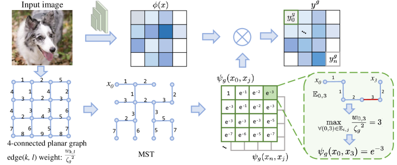
Figure A1: The graphical illustration of the detailed process of global affinity propagation. In the green dashed box, we present the calculation of $\psi_{g}(x_{0},x_{3})$ as a simple example.

Appendix C More Performance Comparisons

For annotation-free semantic segmentation with pretrained CLIP model, Key Smoothing (KS) proposed in MaskCLIP [40] also aims to realize the global affinity propagation. To better explore their efforts, we conduct detailed comparisons between KS and our APro method based on training-free MaskCLIP [40]. The experimental results are shown in Table A1.

Table A1: Quantitative results on Pascal Context [60] val and COCO-Stuff [61] val with mean IoU (%).

Method				CLIP Model	Context	COCO.
MaskCLIP [40]		18.46	10.17
+KS		21.0	12.42
+APro(Ours)	ResNet-50	21.67	12.70
1-4[1pt/1pt] MaskCLIP [40]		21.57	13.55
+KS		22.65	15.50
+APro(Ours)	ResNet-50$\times$16	24.03	16.30
1-4[1pt/1pt] MaskCLIP [40]		21.68	12.51
+KS		23.87	13.79
+KS+PD		25.45	14.62
+APro(Ours)		28.91	16.69
+APro(Ours) +PD	ViT-B/16	29.42	16.71

Both KS and our APro method bring performance gains. Compared with KS, APro achieves better performance with different CLIP-based models. Especially, for ViT-B/16 model, our approach outperforms KS by +5.04% mIoU on Pascal Context and +2.90% mIoU on COCO, repectively. Equipped with Prompt Denoising (PD), the models could achieve further improvements.

We have the following further discussions: KS relies on the calculation of key feature similarities, which predominantly stems from high-level features of CLIP and computes pairwise terms within each pair of patches. Compared with KS of MaskCLIP, our method is built on a tree-based graph derived from low-level images, which is capable of capturing finer topological details.

Appendix D Additional Visualization Results

To further show the performance of our proposed APro approach, we provide more visualization results. Fig. A2 shows the qualitative comparisons with the state-of-the-art methods upon box-supervised instance segmentation task [8, 9, 11]. It can be seen that our proposed APro approach is able to generate more accurate boundaries. For weakly-supervised semantic segmentation, we compare our method with the prior art TEL [7] upon point-wise supervision in Fig. A3. APro captures the fine-grained details of objects with the fitting boundaries. As for CLIP-guided annotation-free semantic segmentation, Fig. A4 provides the comparison results with MaskCLIP+ [40]. It can be observed that our approach eliminates the noisy predictions from the pretrained CLIP model effectively, achieving high-quality mask predictions. In addition, Fig. A5 provides the qualitative results of our method on general COCO dataset.

Appendix E Discussions

Asset License and Consent. We use four image segmentation datasets, i.e., COCO [49], Pascal VOC 2012 [51], COCO-Stuff [61] and Pascal Context [60], which are all publicly and freely available for academic research. We implement all models with MMDetection [56], MMSegmentation [63] and openseg.pytorch [64] codebases. COCO (https://cocodataset.org/) is released under the CC BY 4.0. Pascal VOC 2012 (http://host.robots.ox.ac.uk/pascal/VOC/voc2012/) is released under the Flickr Terms of use for images. COCO-Stuff v1.1 (https://github.com/nightrome/cocostuff) is released under the Flickr Terms of use for images and the CC BY 4.0 for annotations. MMDetection (https://github.com/open-mmlab/mmdetection) and MMSegmentation (https://github.com/open-mmlab/mmsegmentation) codebases are released under the Apache-2.0 license. Openseg.pytorch (https://github.com/openseg-group/openseg. pytorch) codebase is released under the MIT license.

Limitations. The presented affinity propagation method is performed under the guidance of the similarities of image intensity and color. Our proposed method may have difficulties in accurately capturing the pairwise affinities under the challenging scenarios like motion blur, occlusions, and cluttered scenes, etc. Actually, this is a common problem for many segmentation methods. In the future work, we will explore how to integrate our method into the large-scale foundation models, such as SAM [65], to take advantage of their strong features for more promising segmentation results.

Broader Impact. This work presents an effective component for weakly-supervised segmentation with label-efficient annotations. We have demonstrated its effectiveness over three typical label-efficient segmentation tasks. On the positive side, our approach has the potential to benefit a wide variety of real-world applications, such as autonomous vehicles, medical imaging, remote sensing and image editing, which can significantly reduce the labeling costs. On the other side, erroneous predictions in real-world applications (i.e., medical imaging analysis and tasks involving autonomous vehicles) raise the safety issues of human beings. In order to avoid the potentially negative effects, we suggest to adopt a highly stringent security protocol in case that our approach fails to function properly in real-world applications.

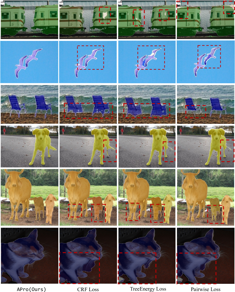
Figure A2: Qualitative comparisons on Pascal VOC [51]. We compare our APro approach with CRF loss [10], TreeEnergy loss [7] and Pairwise loss [8] under the SOLOv2 [52] framework. Our method obtains more fine-grained predictions with detail preserved.

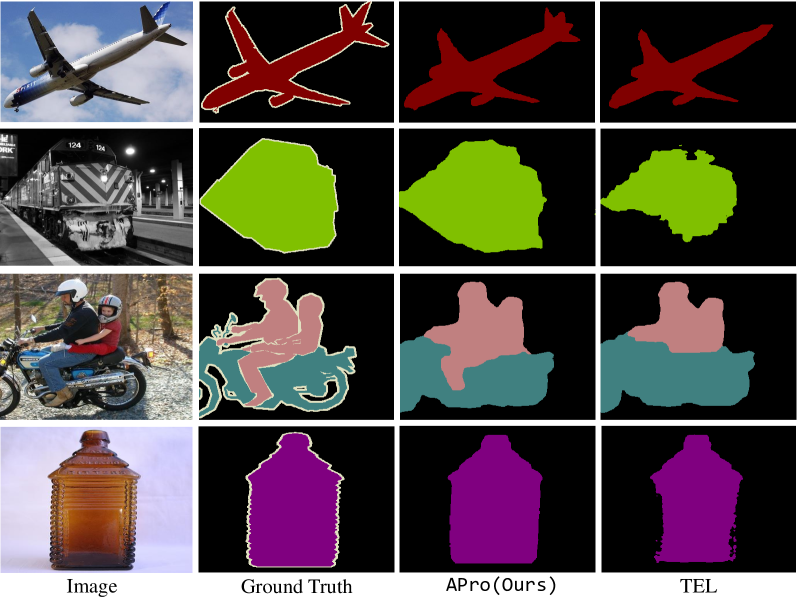
Figure A3: Qualitative comparisons on point-supervised semantic segmentation. Compared with the state-of-the-art TEL [7], our method segments objects with more accurate boundaries.

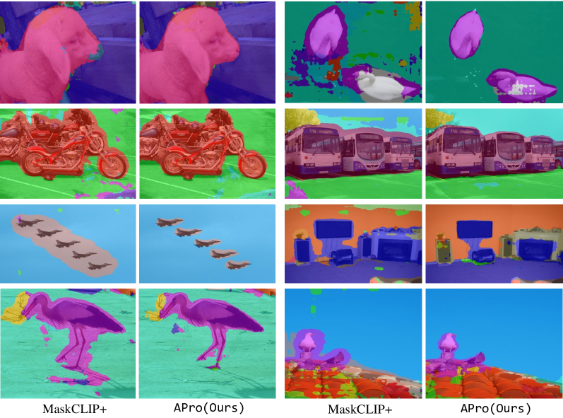
Figure A4: Visual comparison results on Pascal Context with ViT-B/16 image encoder. Compared with the prior art MaskCLIP+ [40], our method obtains more accurate predictions with fitting boundaries.

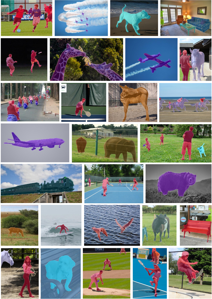
Figure A5: Qualitative results of our APro on COCO with ResNet-101 under the SOLOv2 framework upon box-supervised instance segmentation.

References

- [1] Wei Shen, Zelin Peng, Xuehui Wang, Huayu Wang, Jiazhong Cen, Dongsheng Jiang, Lingxi Xie, Xiaokang Yang, and Q Tian. A survey on label-efficient deep image segmentation: Bridging the gap between weak supervision and dense prediction. TPAMI, 2023.
- [2] Amy Bearman, Olga Russakovsky, Vittorio Ferrari, and Li Fei-Fei. What’s the point: Semantic segmentation with point supervision. In ECCV, pages 549–565, 2016.
- [3] Junsong Fan, Zhaoxiang Zhang, and Tieniu Tan. Pointly-supervised panoptic segmentation. In ECCV, pages 319–336, 2022.
- [4] Wentong Li, Yuqian Yuan, Song Wang, Jianke Zhu, Jianshu Li, Jian Liu, and Lei Zhang. Point2mask: Point-supervised panoptic segmentation via optimal transport. In ICCV, pages 572–581, 2023.
- [5] Di Lin, Jifeng Dai, Jiaya Jia, Kaiming He, and Jian Sun. Scribblesup: Scribble-supervised convolutional networks for semantic segmentation. In CVPR, pages 3159–3167, 2016.
- [6] Meng Tang, Federico Perazzi, Abdelaziz Djelouah, Ismail Ben Ayed, Christopher Schroers, and Yuri Boykov. On regularized losses for weakly-supervised cnn segmentation. In ECCV, pages 507–522, 2018.
- [7] Zhiyuan Liang, Tiancai Wang, Xiangyu Zhang, Jian Sun, and Jianbing Shen. Tree energy loss: Towards sparsely annotated semantic segmentation. In CVPR, pages 16907–16916, 2022.
- [8] Zhi Tian, Chunhua Shen, Xinlong Wang, and Hao Chen. Boxinst: High-performance instance segmentation with box annotations. In CVPR, pages 5443–5452, 2021.
- [9] Wentong Li, Wenyu Liu, Jianke Zhu, Miaomiao Cui, Xian-Sheng Hua, and Lei Zhang. Box-supervised instance segmentation with level set evolution. In ECCV, pages 1–18, 2022.
- [10] Shiyi Lan, Xitong Yang, Zhiding Yu, Zuxuan Wu, Jose M Alvarez, and Anima Anandkumar. Vision transformers are good mask auto-labelers. In CVPR, 2023.
- [11] Wentong Li, Wenyu Liu, Jianke Zhu, Miaomiao Cui, Risheng Yu, Xiansheng Hua, and Lei Zhang. Box2mask: Box-supervised instance segmentation via level-set evolution. arXiv preprint arXiv:2212.01579, 2022.
- [12] Jiwoon Ahn and Suha Kwak. Learning pixel-level semantic affinity with image-level supervision for weakly supervised semantic segmentation. In CVPR, pages 4981–4990, 2018.
- [13] Jiwoon Ahn, Sunghyun Cho, and Suha Kwak. Weakly supervised learning of instance segmentation with inter-pixel relations. In CVPR, pages 2209–2218, 2019.
- [14] Lixiang Ru, Yibing Zhan, Baosheng Yu, and Bo Du. Learning affinity from attention: end-to-end weakly-supervised semantic segmentation with transformers. In CVPR, pages 16846–16855, 2022.
- [15] Jinlong Li, Zequn Jie, Xu Wang, Xiaolin Wei, and Lin Ma. Expansion and shrinkage of localization for weakly-supervised semantic segmentation. In NeurIPS, 2022.
- [16] Cheng-Chun Hsu, Kuang-Jui Hsu, Chung-Chi Tsai, Yen-Yu Lin, and Yung-Yu Chuang. Weakly supervised instance segmentation using the bounding box tightness prior. In NeurIPS, volume 32, 2019.
- [17] Shiyi Lan, Zhiding Yu, Christopher Choy, Subhashree Radhakrishnan, Guilin Liu, Yuke Zhu, Larry S Davis, and Anima Anandkumar. Discobox: Weakly supervised instance segmentation and semantic correspondence from box supervision. In ICCV, pages 3406–3416, 2021.
- [18] Paul Vernaza and Manmohan Chandraker. Learning random-walk label propagation for weakly-supervised semantic segmentation. In CVPR, pages 7158–7166, 2017.
- [19] Lin Song, Yanwei Li, Zeming Li, Gang Yu, Hongbin Sun, Jian Sun, and Nanning Zheng. Learnable tree filter for structure-preserving feature transform. In NeurIPS, volume 32, 2019.
- [20] Joseph B Kruskal. On the shortest spanning subtree of a graph and the traveling salesman problem. Proceedings of the American Mathematical society, 7(1):48–50, 1956.
- [21] Lin Song, Yanwei Li, Zhengkai Jiang, Zeming Li, Xiangyu Zhang, Hongbin Sun, Jian Sun, and Nanning Zheng. Rethinking learnable tree filter for generic feature transform. In NeurIPS, volume 33, pages 3991–4002, 2020.
- [22] Xiaojin Zhu, Zoubin Ghahramani, and John D Lafferty. Semi-supervised learning using gaussian fields and harmonic functions. In ICML, pages 912–919, 2003.
- [23] Xiaojin Zhu. Semi-supervised learning literature survey. 2005.
- [24] Alexander Vezhnevets and Joachim M Buhmann. Towards weakly supervised semantic segmentation by means of multiple instance and multitask learning. In CVPR, pages 3249–3256, 2010.
- [25] Deepak Pathak, Evan Shelhamer, Jonathan Long, and Trevor Darrell. Fully convolutional multi-class multiple instance learning. arXiv preprint arXiv:1412.7144, 2014.
- [26] Deepak Pathak, Philipp Krahenbuhl, and Trevor Darrell. Constrained convolutional neural networks for weakly supervised segmentation. In ICCV, pages 1796–1804, 2015.
- [27] Pedro O Pinheiro and Ronan Collobert. From image-level to pixel-level labeling with convolutional networks. In CVPR, pages 1713–1721, 2015.
- [28] George Papandreou, Liang-Chieh Chen, Kevin P Murphy, and Alan L Yuille. Weakly-and semi-supervised learning of a deep convolutional network for semantic image segmentation. In ICCV, pages 1742–1750, 2015.
- [29] Ruihuang Li, Chenhang He, Yabin Zhang, Shuai Li, Liyi Chen, and Lei Zhang. Sim: Semantic-aware instance mask generation for box-supervised instance segmentation. In CVPR, 2023.
- [30] Tianheng Cheng, Xinggang Wang, Shaoyu Chen, Qian Zhang, and Wenyu Liu. Boxteacher: Exploring high-quality pseudo labels for weakly supervised instance segmentation. In CVPR, 2023.
- [31] Rui Yang, Lin Song, Yixiao Ge, and Xiu Li. Boxsnake: Polygonal instance segmentation with box supervision. In ICCV, 2023.
- [32] Bowen Cheng, Omkar Parkhi, and Alexander Kirillov. Pointly-supervised instance segmentation. In CVPR, pages 2617–2626, 2022.
- [33] Chufeng Tang, Lingxi Xie, Gang Zhang, Xiaopeng Zhang, Qi Tian, and Xiaolin Hu. Active pointly-supervised instance segmentation. In ECCV, pages 606–623, 2022.
- [34] Hongjun Chen, Jinbao Wang, Hong Cai Chen, Xiantong Zhen, Feng Zheng, Rongrong Ji, and Ling Shao. Seminar learning for click-level weakly supervised semantic segmentation. In ICCV, pages 6920–6929, 2021.
- [35] Bingfeng Zhang, Jimin Xiao, Jianbo Jiao, Yunchao Wei, and Yao Zhao. Affinity attention graph neural network for weakly supervised semantic segmentation. TPAMI, 44(11):8082–8096, 2021.
- [36] Dmitrii Marin, Meng Tang, Ismail Ben Ayed, and Yuri Boykov. Beyond gradient descent for regularized segmentation losses. In CVPR, pages 10187–10196, 2019.
- [37] Yun Liu, Yu-Huan Wu, Peisong Wen, Yujun Shi, Yu Qiu, and Ming-Ming Cheng. Leveraging instance-, image-and dataset-level information for weakly supervised instance segmentation. TPAMI, 44(3):1415–1428, 2020.
- [38] Alec Radford, Jong Wook Kim, Chris Hallacy, Aditya Ramesh, Gabriel Goh, Sandhini Agarwal, Girish Sastry, Amanda Askell, Pamela Mishkin, Jack Clark, et al. Learning transferable visual models from natural language supervision. In ICML, pages 8748–8763, 2021.
- [39] Yuqi Lin, Minghao Chen, Wenxiao Wang, Boxi Wu, Ke Li, Binbin Lin, Haifeng Liu, and Xiaofei He. Clip is also an efficient segmenter: A text-driven approach for weakly supervised semantic segmentation. In CVPR, 2023.
- [40] Chong Zhou, Chen Change Loy, and Bo Dai. Extract free dense labels from clip. In ECCV, pages 696–712, 2022.
- [41] Yanwei Li, Hengshuang Zhao, Xiaojuan Qi, Yukang Chen, Lu Qi, Liwei Wang, Zeming Li, Jian Sun, and Jiaya Jia. Fully convolutional networks for panoptic segmentation with point-based supervision. TPAMI, 2022.
- [42] Philipp Krähenbühl and Vladlen Koltun. Efficient inference in fully connected crfs with gaussian edge potentials. In NeurIPS, volume 24, 2011.
- [43] Liang-Chieh Chen, George Papandreou, Iasonas Kokkinos, Kevin Murphy, and Alan L Yuille. Deeplab: Semantic image segmentation with deep convolutional nets, atrous convolution, and fully connected crfs. TPAMI, 40(4):834–848, 2017.
- [44] Shuai Zheng, Sadeep Jayasumana, Bernardino Romera-Paredes, Vibhav Vineet, Zhizhong Su, Dalong Du, Chang Huang, and Philip HS Torr. Conditional random fields as recurrent neural networks. In ICCV, pages 1529–1537, 2015.
- [45] Anton Obukhov, Stamatios Georgoulis, Dengxin Dai, and Luc Van Gool. Gated crf loss for weakly supervised semantic image segmentation. In NeurIPS, 2019.
- [46] William T Freeman, Egon C Pasztor, and Owen T Carmichael. Learning low-level vision. IJCV, 40:25–47, 2000.
- [47] Qingxiong Yang. Stereo matching using tree filtering. IEEE TPAMI, 37(4):834–846, 2014.
- [48] Robert Endre Tarjan. A class of algorithms which require nonlinear time to maintain disjoint sets. Journal of computer and system sciences, 18(2):110–127, 1979.
- [49] Tsung-Yi Lin, Michael Maire, Serge Belongie, James Hays, Pietro Perona, Deva Ramanan, Piotr Dollár, and C Lawrence Zitnick. Microsoft coco: Common objects in context. In ECCV, pages 740–755, 2014.
- [50] Bharath Hariharan, Pablo Arbeláez, Lubomir Bourdev, Subhransu Maji, and Jitendra Malik. Semantic contours from inverse detectors. In ICCV, pages 991–998, 2011.
- [51] Mark Everingham, Luc Van Gool, Christopher KI Williams, John Winn, and Andrew Zisserman. The pascal visual object classes (voc) challenge. IJCV, 88(2):303–338, 2010.
- [52] Xinlong Wang, Rufeng Zhang, Tao Kong, Lei Li, and Chunhua Shen. Solov2: Dynamic and fast instance segmentation. In NeurIPS, volume 33, pages 17721–17732, 2020.
- [53] Bowen Cheng, Ishan Misra, Alexander G Schwing, Alexander Kirillov, and Rohit Girdhar. Masked-attention mask transformer for universal image segmentation. In CVPR, pages 1290–1299, 2022.
- [54] Kaiming He, Xiangyu Zhang, Shaoqing Ren, and Jian Sun. Deep residual learning for image recognition. In CVPR, pages 770–778, 2016.
- [55] Ze Liu, Yutong Lin, Yue Cao, Han Hu, Yixuan Wei, Zheng Zhang, Stephen Lin, and Baining Guo. Swin transformer: Hierarchical vision transformer using shifted windows. In ICCV, pages 10012–10022, 2021.
- [56] Kai Chen, Jiaqi Wang, Jiangmiao Pang, Yuhang Cao, Yu Xiong, Xiaoxiao Li, Shuyang Sun, Wansen Feng, Ziwei Liu, Jiarui Xu, et al. Mmdetection: Open mmlab detection toolbox and benchmark. arXiv preprint arXiv:1906.07155, 2019.
- [57] Olga Russakovsky, Jia Deng, Hao Su, Jonathan Krause, Sanjeev Satheesh, Sean Ma, Zhiheng Huang, Andrej Karpathy, Aditya Khosla, Michael Bernstein, et al. Imagenet: large scale visual recognition challenge. IJCV, 115:211–252, 2015.
- [58] Golnaz Ghiasi, Yin Cui, Aravind Srinivas, Rui Qian, Tsung-Yi Lin, Ekin D Cubuk, Quoc V Le, and Barret Zoph. Simple copy-paste is a strong data augmentation method for instance segmentation. In CVPR, pages 2918–2928, 2021.
- [59] Meng Tang, Abdelaziz Djelouah, Federico Perazzi, Yuri Boykov, and Christopher Schroers. Normalized cut loss for weakly-supervised cnn segmentation. In CVPR, pages 1818–1827, 2018.
- [60] Roozbeh Mottaghi, Xianjie Chen, Xiaobai Liu, Nam-Gyu Cho, Seong-Whan Lee, Sanja Fidler, Raquel Urtasun, and Alan Yuille. The role of context for object detection and semantic segmentation in the wild. In CVPR, pages 891–898, 2014.
- [61] Holger Caesar, Jasper Uijlings, and Vittorio Ferrari. Coco-stuff: Thing and stuff classes in context. In CVPR, 2018.
- [62] Alexey Dosovitskiy, Lucas Beyer, Alexander Kolesnikov, Dirk Weissenborn, Xiaohua Zhai, Thomas Unterthiner, Mostafa Dehghani, Matthias Minderer, Georg Heigold, Sylvain Gelly, et al. An image is worth 16x16 words: Transformers for image recognition at scale. In ICLR, 2020.
- [63] MMSegmentation Contributors. MMSegmentation: Openmmlab semantic segmentation toolbox and benchmark. https://github.com/open-mmlab/mmsegmentation, 2020.
- [64] openseg.pytorch Contributors. openseg.pytorch. https://github.com/openseg-group/openseg.pytorch, 2020.
- [65] Alexander Kirillov, Eric Mintun, Nikhila Ravi, Hanzi Mao, Chloe Rolland, Laura Gustafson, Tete Xiao, Spencer Whitehead, Alexander C Berg, Wan-Yen Lo, et al. Segment anything. arXiv preprint arXiv:2304.02643, 2023.