Pattern-detection in the global automotive industry:
a manufacturer-supplier-product network analysis

Abstract

Production networks arise from supply and customer relations among firms. These systems are nowadays gaining attention as a consequence of the supply chain disruptions due to natural or man-made disasters that happened in the last few years, such as the Covid-19 pandemic or the Russia-Ukraine war. Recent empirical evidence shows that production networks are shaped by functional modules arising from ‘complementary relationships’ between firms. However, data constraints force the few, available studies to consider only country-specific production networks. In order to fully capture the cross-country structure of modern supply chains, here we focus on the global automotive industry as represented by the ‘MarkLines Automotive’ dataset. After representing this data as a network of manufacturers, suppliers, and products, we perform a pattern-detection exercise using a statistically grounded validation technique based on the maximum entropy principle. We reveal the presence of a significantly large number of V-shaped and square-shaped motifs, indicating that manufacturing firms compete and are seldom engaged in a buyer-supplier relationship, while they typically have many suppliers in common. Interestingly, ‘generalist’ and ‘specialist’ suppliers coexist in the network. Additionally, we unveil the presence of geographical patterns, with manufacturers clustering around groups of suppliers; for instance, Chinese firms constitute a disconnected community, likely an effect of the protectionist policies promoted by the Chinese government. We also show the tendency of suppliers to organize their production by targeting specific ‘functional modules’ of a vehicle. Besides shedding light on the self-organising principles shaping production networks, our findings open up the possibility of designing realistic generative models of supply chains, to be used for testing the resilience of the interconnected global economy.

I Introduction

The growth of network science over the last twenty years has impacted several disciplines, by establishing new empirical facts about the structural properties of complex systems as well as novel methodologies for their analysis. Prominent examples are represented by economic and financial networks, such as international trade [1, 2, 3], country-product exporting relationships [4, 5, 6, 7] transaction networks [8, 9] and, after the 2008 global financial crisis, interbank networks [10, 11, 12, 13, 14].

A class of systems that has recently gained attention is that of interfirm production networks, or supply chains, emerging as (manufacturing) firms become dependent on other (supplier) firms for their own production. As a consequence of globalization [15] and of a constant strive towards efficiency [16], production networks have become increasingly interdependent – a feature lying at the basis of the business interruptions that occurred due to recent natural and man-made disasters, such as (the first wave of) the Covid-19 pandemic [17, 18, 19, 20, 21, 22]. The propagation of shocks through an economy has been traditionally studied using classical input-output economics at the industry level [23]. However, economists have recently pointed out the importance of considering supply chain data at the firm level, in particular to assess the consequences of individual firm failures on macroeconomic fluctuations [24, 25, 26], also because data aggregation can create substantial biases [27, 28]. Indeed, the importance of considering the microscopic topology of the network to understand its resilience to shocks has been extensively demonstrated in the financial network literature [29]. Therefore, network theory is becoming increasingly popular as a tool to analyse production systems at the firm level [30, 31, 32, 33, 34, 35, 36], study the propagation of shocks and estimate supply chain resilience [37, 38, 39, 40, 41].

Firm-level datasets are notoriously difficult to acquire because of both technical and privacy issues [42]. While early works relied on aggregated flows of goods between countries [43, 44, 45, 46, 47], today there are a few firm-level datasets with global coverage that are built from financial reports, but mainly cover large companies listed on US stock exchanges and their main customers: this is the case of Factset [48, 42], Compustat [49, 50, 37] and Capital IQ [51, 52] data. Other global datasets that have been analyzed in the Operations Research and Supply Chain Management literature concern specific industrial sectors [53]. The most popular and complete data is about the automotive sector, obtained from a private industry database (the ‘MarkLines Automotive Information Platform’) populated through surveys sent to automotive supplier firms [54, 55]. At the individual country level, instead, production networks can be constructed either from value-added tax (VAT) data concerning the transactions between the firms registered in a country (examples are provided by Belgium [56], Ecuador [57], Hungary [40], Spain [58]) or from payment data provided by central, or major, banks (examples are provided by Brazil [59], Japan [60, 61] and The Netherlands [62]). National data, often characterised by a reporting threshold, typically have a very good internal coverage although do not contain information about international relationships.

The Japan Interfirm Network (JIN) was the first large-scale dataset at the firm level to become available, hence being extensively studied during the last decade [63, 64, 60, 61, 65]. Empirical analyses of the JIN revealed that firm-specific structural quantities (such as the number of connections), as well as purely financial indicators (for instance the total amount of sales and the total number of employees) are distributed as power-laws, while firm degree grows along with its total sales in a non-linear fashion [63]. Regarding the JIN topology, it was shown to be disassortative by degree (as suppliers with few customers are preferentially connected with large firms) and characterised by a well-defined community structure, with clusters being shaped by geographic proximity and industrial sector similarity [61]: notably, these clusters are characterized by bipartite structures with large companies not being directly linked but sharing many first-tier suppliers. This result was confirmed by a comprehensive study of triadic motifs [60]: when compared with a benchmark constraining the degree of each firm, the JIN features an over-representation of V-shaped motifs [3] and an under-representation of triangular loops.

These findings have been interpreted as a sign that the self-organization of production networks is driven by complementarity rather than homophily [66]. Indeed the latter is known to play an important role in shaping social networks, where people with similar interests or acquaintances are likely to be connected, causing the formation of a large number of closed triangles - a tendency well summed up by the popular saying ‘the friend of my friend is my friend as well’ [67]. However, networks in different contexts can obey different principles: two proteins with similar binding sites do not interact directly but can be both linked with others having complementary binding properties; protein interaction networks are thus characterised by a large number of square patterns [68]. As the over-representation of V-shaped motifs characterizing the JIN is compatible with the over-representation of the square patterns known as X-motifs [3], the findings of [61, 60] corroborate a similar picture, according to which firms with similar outputs are often engaged in a competitive (rather than a buyer-supplier) relationship, but can have many suppliers and customers in common [55].

Such an over-representation of square motifs has been explicitly shown only for a company-level production network constructed from Dutch national economic statistics [69, 66]: no results are available for global datasets, despite the well-documented cross-country structure of production networks [15]. The aim of this paper is to bridge the gap by carrying out a pattern-detection analysis on a global scale, using the ‘MarkLines Automotive’ dataset. In particular, after providing a representation of the system in terms of a manufacturer-supplier-product network, we employ validation techniques based on the maximum-entropy principle to unveil the presence of statistically significant patterns [3, 70, 71].

Table 1: Basic statistics of the ‘MarkLines Automotive’ dataset for each category of products: Chassis/Body (CB), Electrical (EL), Powertrain (PW), Interior/Exterior (IE) and General parts (GP). The percentages reported in the last row are so small to let us opt for discarding the links between manufacturers, hence obtaining perfectly bipartite networks.

	CB	EL	PW	IE	GP	Full
# manufacturers	246	215	249	196	108	301
# suppliers	1864	1203	2659	1776	479	5725
# links	7937	5390	10978	6502	1687	26535
% internal links	0.4	0.94	2.6	0.83	0	1.3

II Methods

II.1 Network representation of the ‘MarkLines Automotive’ dataset

According to the (technological) taxonomy provided by the platform https://www.marklines.com, products are classified into five categories: Chassis/Body (CB), Electrical (EL), Powertrain (PW), Interior/Exterior (IE) and General parts (GP). A thorough data-cleaning and harmonization procedure (see also Appendix A) has led us to consider $M=301$ manufacturers, $S=5.725$ suppliers, and $P=291$ products; the overall number of buyer-supplier relationships amounts to $26.535$ (see also table 1).

Information about each category of products, indexed by $\gamma=1\dots 5$, can be arranged into a biadjacency matrix $\mathbf{B}^{\gamma}$ whose dimensions read $M^{\gamma}\times S^{\gamma}$, where $M^{\gamma}$ is the number of manufacturers and $S^{\gamma}$ is the number of suppliers in category $\gamma$: naturally, $b_{ms}^{\gamma}=1$ if supplier $s$ provides manufacturer $m$ with at least one product belonging to category $\gamma$ and $b_{ms}^{\gamma}=0$ otherwise. Overall, then, the ‘MarkLines Automotive’ dataset can be represented as a bipartite multiplex, each layer corresponding to a category of technological products (see also the left panel of figure 1).

Alternatively, the dataset can be represented as an $M\times S\times P$ tripartite network, i.e. a ‘combination’ of two bipartite networks sharing the set of suppliers (see also the right panel of figure 1): the generic element of the ‘left’ $M\times S$ biadjacency matrix $\mathbf{L}$ reads $l_{ms}=1$ if manufacturer $m$ buys from supplier $s$, otherwise $l_{ms}=0$; analogously, the generic element of the ‘right’ $S\times P$ biadjacency matrix $\mathbf{R}$ reads $r_{sp}=1$ if supplier $s$ sells product $p$ and $r_{sp}=0$ otherwise. Although we could also link each manufacturer to the set of products purchased by its suppliers, the evidence that all of them are car producers and hence need the same basket of products let us opt for discarding this third set of connections.

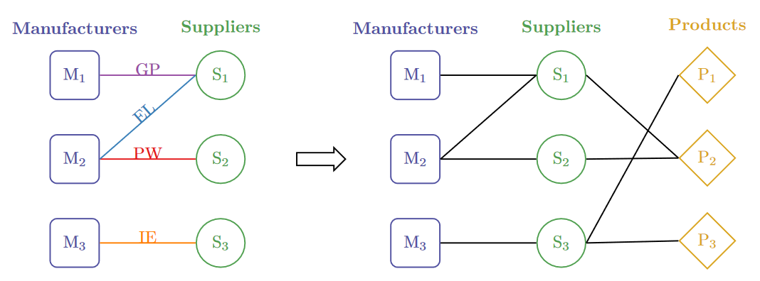
Figure 1: The ‘MarkLines Automotive’ dataset, represented either as a bipartite multiplex (left panel) or as a tripartite network (right panel).

II.2 Structural properties

Local connectivity.

The most important network quantity at the local level is the degree, defined as the number of connections of a node. In order to properly describe our data, we need the following definitions:

• the number of suppliers, or product providers, of manufacturer $m$: $k_{m\rightarrow\mathcal{S}}=\sum_{s=1}^{S}l_{ms}$;

• the number of customers, or client manufacturers, of supplier $s$: $k_{s\rightarrow\mathcal{M}}=\sum_{m=1}^{M}l_{ms}$;

• the ‘diversification’ of supplier $s$, i.e. the number of products it sells to its client manufacturers: $k_{s\rightarrow\mathcal{P}}=\sum_{p=1}^{P}r_{sp}$;

• the ‘ubiquity’ of product $p$, i.e. the number of its vendor suppliers: $k_{p\rightarrow\mathcal{S}}=\sum_{s=1}^{S}r_{sp}$.

Assortativity.

The presence of degree correlations is captured by the average nearest neighbors’ degree. In order to properly describe our data, we need the following definitions:

• the average number of customers of a manufacturer’s neighbors: $\text{ANND}_{m\rightarrow\mathcal{S}}=\sum_{s=1}^{S}l_{ms}k_{s\rightarrow\mathcal{M}}/k_{m\rightarrow\mathcal{S}}$;

• the average number of providers of a supplier’s neighbors: $\text{ANND}_{s\rightarrow\mathcal{M}}=\sum_{m=1}^{M}l_{ms}k_{m\rightarrow\mathcal{S}}/k_{s\rightarrow\mathcal{M}}$;

• the average ‘ubiquity’ of a supplier’s products: $\text{ANND}_{s\rightarrow\mathcal{P}}=\sum_{p=1}^{P}r_{sp}k_{p\rightarrow\mathcal{S}}/k_{s\rightarrow\mathcal{P}}$;

• the average ‘diversification’ of a product’s suppliers: $\text{ANND}_{p\rightarrow\mathcal{S}}=\sum_{s=1}^{S}r_{sp}k_{s\rightarrow\mathcal{P}}/k_{p\rightarrow\mathcal{S}}$.

Motifs.

In order to capture the concept of a node’s ‘highly connected neighborhood’, we need to consider the bipartite analogue of the monopartite square clustering coefficient. To this aim, several definitions have been proposed so far (see also Appendix B): here, we adopt the one provided in [72] and reading

$$\text{BCC}_{m}=\frac{\sum_{s<s^{\prime}}q_{m}(s,s^{\prime})}{\sum_{s<s^{\prime}}[(k_{s\rightarrow\mathcal{M}}-1)+(k_{s^{\prime}\rightarrow\mathcal{M}}-1)-q_{m}(s,s^{\prime})]}$$ (1)

where $k_{s\rightarrow\mathcal{M}}$ is the number of customers, or client manufacturers, of supplier $s$ and

$$q_{m}(s,s^{\prime})=\sum_{\begin{subarray}{c}m^{\prime}=1\\ (m^{\prime}\neq m)\end{subarray}}^{M}l_{ms}l_{ms^{\prime}}l_{m^{\prime}s}l_{m^{\prime}s^{\prime}}=l_{ms}l_{ms^{\prime}}\sum_{\begin{subarray}{c}m^{\prime}=1\\ (m^{\prime}\neq m)\end{subarray}}^{M}l_{m^{\prime}s}l_{m^{\prime}s^{\prime}}$$ (2)

counts the number of cycles, composed by four links, involving the common neighbors to $s$ and $s^{\prime}$, other than $m$. According to $\text{BCC}_{m}$, the total number of closed squares involving manufacturer $m$ is given by the sum of degrees of all pairs of its neighbours minus $q_{m}(s,s^{\prime})$, i.e. the number of squares that are already closed. In other words, the total number of closed squares coincides with the number of squares that could become closed upon connecting, by adding new links, the neighbors of $s$ with $s^{\prime}$ and the neighbors of $s^{\prime}$ with $s$, excluding $m$ from both sets.

Upon considering that the generic addendum $l_{ms}l_{ms^{\prime}}l_{m^{\prime}s}l_{m^{\prime}s^{\prime}}$ equals 1 if a closed square involving nodes $m$, $m^{\prime}$, $s$ and $s^{\prime}$ exists and 0 otherwise, we can compute the number of squares involving manufacturers $m$ and $m^{\prime}$ by summing over $s$ and $s^{\prime}$, i.e. as

$$X_{mm^{\prime}}=\sum_{s<s^{\prime}}l_{ms}l_{ms^{\prime}}l_{m^{\prime}s}l_{m^{\prime}s^{\prime}}=\binom{V_{mm^{\prime}}}{2}$$ (3)

where $V_{mm^{\prime}}\equiv\sum_{s=1}^{S}l_{ms}l_{m^{\prime}s}$ is the number of common suppliers (V-motifs) to $m$ and $m^{\prime}$ [3]: hence, the number of cycles, composed by four links, involving node $m$ equals the number of X-motifs involving it, i.e. $\sum_{s<s^{\prime}}q_{m}(s,s^{\prime})=\sum_{\begin{subarray}{c}m^{\prime}=1\\ (m^{\prime}\neq m)\end{subarray}}^{M}X_{mm^{\prime}}$.

Subgraph centrality.

In order to detect the presence of closed paths of higher order, we have considered the bipartite analogue of the monopartite subgraph centrality [73], whose definition reads

$$\text{BSC}_{m}=\frac{\sum_{k=0}^{\infty}[\mathbf{L}^{2k}]_{mm}}{(2k)!}=[\text{cosh}(\mathbf{L})]_{mm}$$ (4)

where $\mathbf{L}^{0}\equiv\mathbf{I}$, i.e., the zeroth power of $\mathbf{L}$ coincides with the $M\times M$ identity matrix, and only closed walks of even length are accounted for. Still, carrying out a meaningful comparison of the centrality of nodes across different configurations requires it to be properly normalized; here, we adopt the following definition

$$\overline{\text{BSC}}_{m}=\frac{\text{BSC}_{m}}{\sum_{m=1}^{M}\text{BSC}_{m}}=\frac{[\text{cosh}(\mathbf{L})]_{mm}}{\text{Tr}[\text{cosh}(\mathbf{L})]}.$$ (5)

II.3 Statistical benchmarks

Answering the question of whether an empirical property represents a non-trivial signature of a network requires comparing it with a properly defined benchmark - or null model, as its role is analogous to the one played by a null hypothesis in traditional statistics.

Following the approach introduced in [74] and developed in [75], here we adopt the Exponential Random Graphs (ERG) formalism, characterizing maximum-entropy probability distributions that preserve a desired set of constraints on average while keeping everything else as random as possible [76]. Among the models that can be defined within this framework, we consider the Bipartite Configuration Model (BiCM), introduced in [3] and defined by constraining the degrees of the nodes belonging to both layers of a bipartite network - in other words, this model embodies the null hypothesis that (the numerical values of) empirical network patterns are induced by (the numerical values of) the degrees of the nodes.

Let us, now, briefly illustrate the basic results for our manufacturer-supplier network, redirecting the interested reader to [3] for the explicit derivation of the BiCM. In the case of the BiCM, constrained entropy-maximization leads to a factorized probability reading $P(\mathbf{L})=\prod_{m,s}p_{ms}^{l_{ms}}(1-p_{ms})^{1-l_{ms}}$ where

$$p_{ms}=\frac{x_{m}y_{s}}{1+x_{m}y_{s}}$$ (6)

is the probability that manufacturer $m$ and supplier $s$ are connected (i.e. that $l_{ms}=1$) and $x_{m}$ and $y_{s}$ are functions of the Lagrange multipliers, respectively controlling for the degrees $k_{m\rightarrow S}$ and $k_{s\rightarrow M}$.

The vectors of parameters $\bm{x}$ and $\bm{y}$ must be numerically determined: here, we employ the maximum likelihood principle, prescribing to maximize the expression $\mathscr{L}=\ln P(\mathbf{L}|\bm{x},\bm{y})$ with respect to $x_{m}$, $\forall\>m$ and $y_{s}$, $\forall\>s$. Such a recipe leads us to find the system of equations

$$k_{m\rightarrow S}^{*} =\sum_{s=1}^{S}\frac{x_{m}y_{s}}{1+x_{m}y_{s}},\>\forall\>m$$ (7)

$$k_{s\rightarrow M}^{*} =\sum_{m=1}^{M}\frac{x_{m}y_{s}}{1+x_{m}y_{s}},\>\forall\>s$$ (8)

ensuring that the empirical value of each constraint matches its expectation. The system above has been solved by running the NEMTROPY package [71] available at https://github.com/nicoloval/NEMtropy.

II.4 Projection of the ‘MarkLines Automotive’ dataset

The projection of a bipartite network onto one of its layers yields a monopartite graph, where each pair of nodes is connected as the number of common neighbors, proxying their similarity [77, 78], is significantly large. Here, we follow the approach proposed in [79, 70] to validate the similarity of any two nodes with respect to the BiCM. Schematically, this method works by A) focusing on a specific pair of nodes belonging to the layer of interest and counting the number of common neighbors; B) quantifying its statistical significance with respect to the BiCM; C) linking the two nodes if, and only if, the corresponding p-value is sufficiently low. Let us now describe these steps in detail.

Quantifying nodes similarity.

The simplest indicator of the similarity of two nodes belonging to the same layer of a bipartite network is provided by the number of their common neighbors. For the couple of manufacturers $m$ and $m^{\prime}$ this number is given by

$$V_{mm^{\prime}}^{*}=\sum_{s=1}^{S}l_{ms}l_{m^{\prime}s},$$ (9)

i.e. the number of V-motifs the two nodes originate - as $m$ and $m^{\prime}$ cannot be directly connected, the presence of a common supplier, belonging to the opposite layer, draws a V-like shape [70].

Statistical significance of nodes similarity.

The BiCM, as any ERG model induced by linear constraints, treats links as independent random variables. Therefore, the presence of a common supplier for any two manufacturers $m$ and $m^{\prime}$, i.e. $l_{ms}l_{m^{\prime}s}=1$, can be described as the outcome of a Bernoulli trial whose probability coefficients read:

$$f_{\text{Ber}}(l_{ms}l_{m^{\prime}s})=p_{ms}p_{m^{\prime}s},$$ (10)

$$f_{\text{Ber}}(l_{ms}l_{m^{\prime}s}=0)=1-p_{ms}p_{m^{\prime}s}.$$ (11)

As $V_{mm^{\prime}}$ is a sum of independent Bernoulli trials, each characterized by a different probability, the behaviour of such a random variable is described by the Poisson-Binomial (PB) distribution [70]. Evaluating the statistical significance of the similarity of nodes $m$ and $m^{\prime}$, thus, amounts at computing the p-value

$$\text{p-value}(V_{mm^{\prime}})=\sum_{x\geq V_{mm^{\prime}}^{*}}f_{\text{PB}}(x).$$ (12)

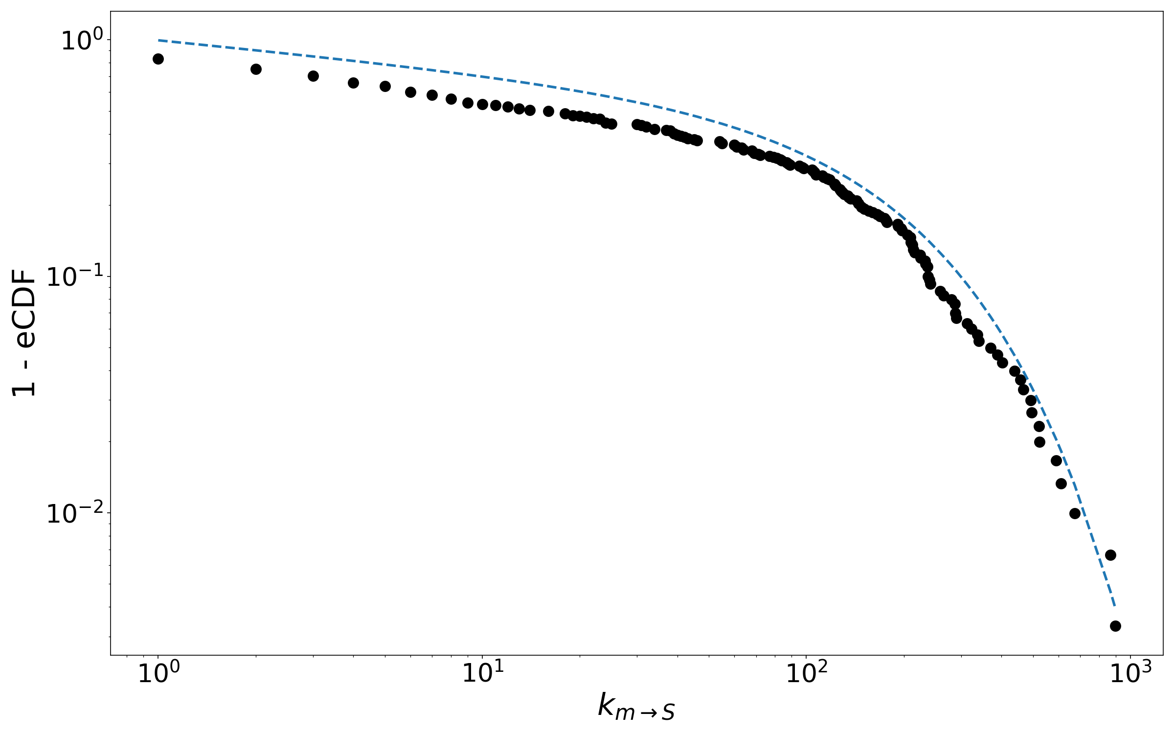
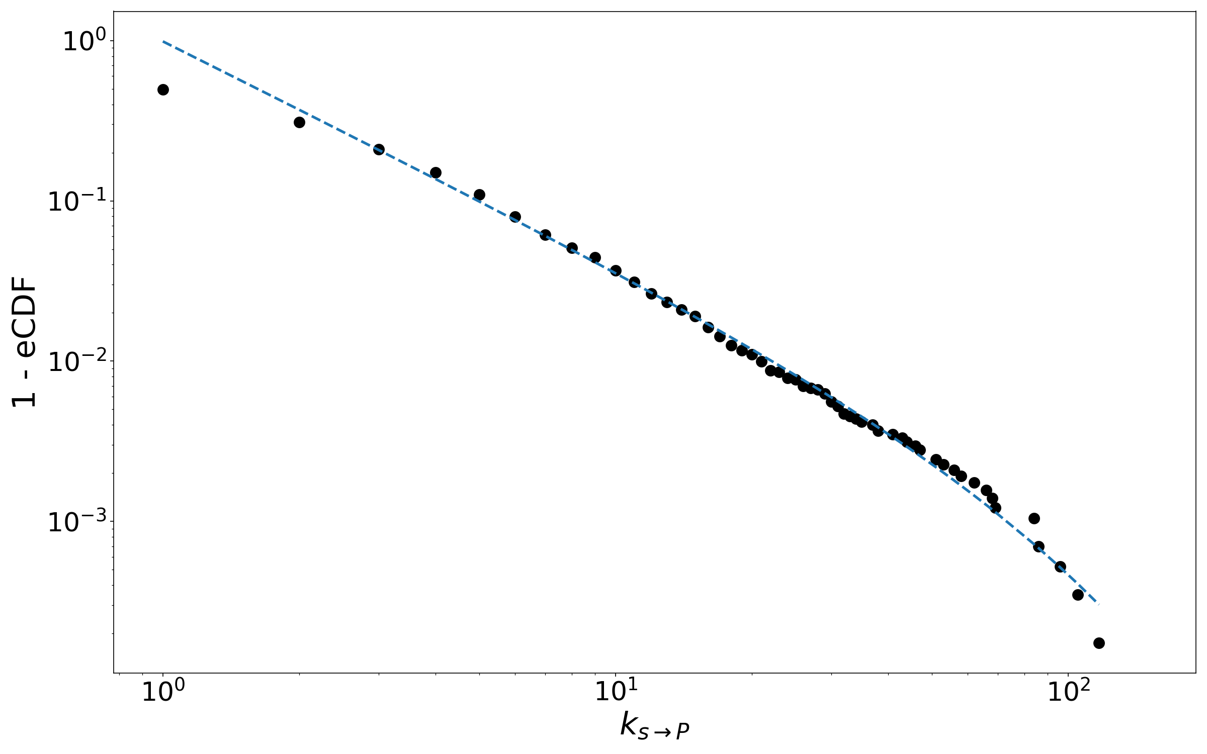
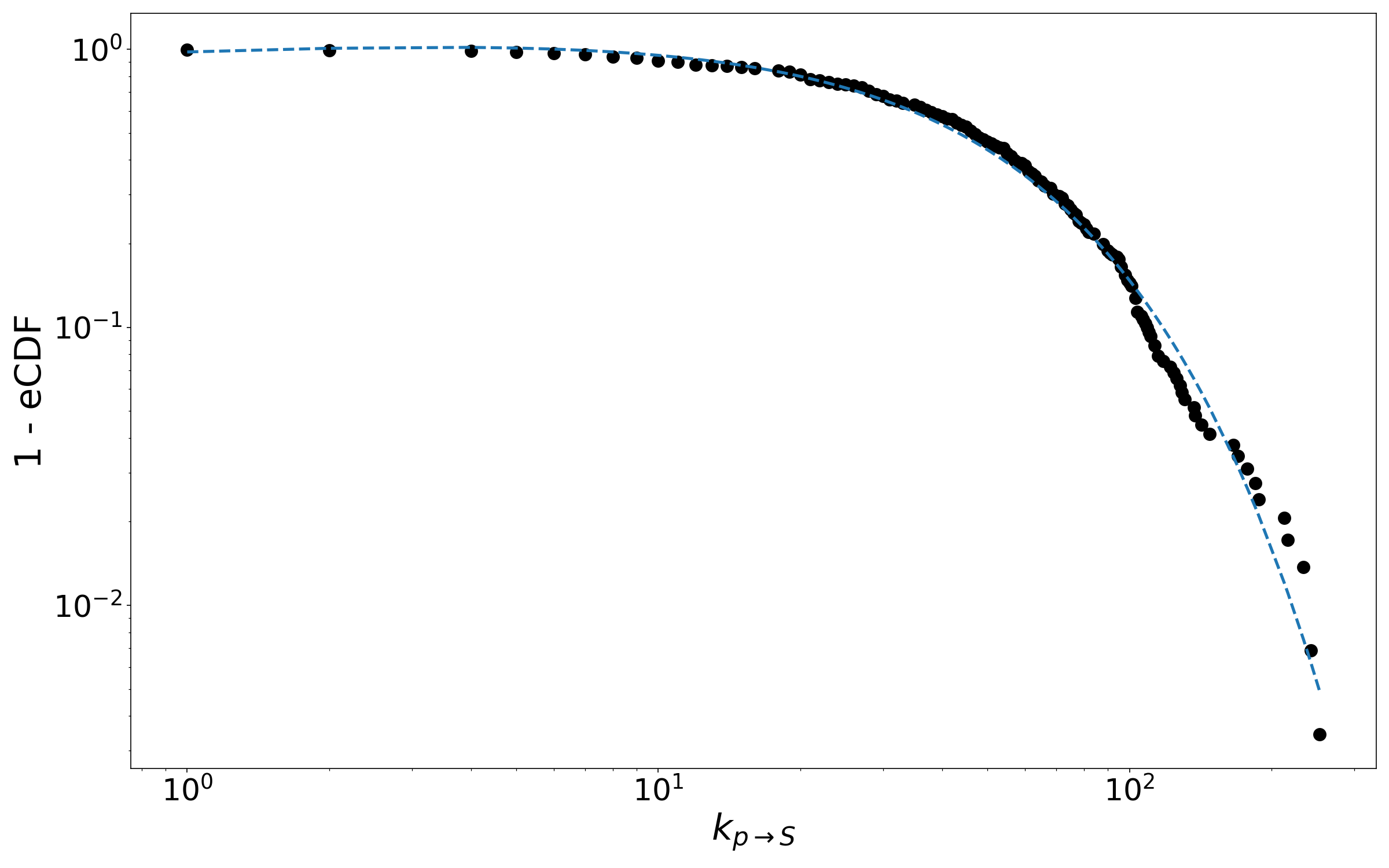
Figure 2: Empirical cumulative density function of manufacturers’ degrees (top left), suppliers’ ‘left’ degrees (top right), suppliers’ ‘right’ degrees (bottom left) and products’ degrees (bottom right): all of them are heavy-tailed and right-skewed, a result pointing out the quite large heterogeneity of our nodes connectivity. More specifically, they all obey a power-law with exponential cutoff whose functional form reads $f(x)=x^{-\alpha}e^{-\beta x}\beta^{1-\alpha}/\Gamma[1-\alpha,\beta x_{\text{min}}]$ and whose parameters - numerically determined by implementing the Levenberg-Marquardt algorithm [80] for least squares optimization through the Python library SciPy - read $\alpha=0.134$, $\beta=0.005$ (top left), $\alpha=0.743$, $\beta=0.049$ (top right), $\alpha=1.276$, $\beta=0.015$ (bottom left), $\alpha=0.063$, $\beta=0.022$ (bottom right). Overall, the above results indicate that ‘generalist’ suppliers co-exist with ‘specialist’ suppliers - noticeably, $\simeq 51\%$ of suppliers sells only one product.

Validating the monopartite projection.

P-values must, then, be validated by implementing a procedure for testing multiple hypotheses at a time. Several alternatives are viable, among which the Bonferroni correction [81], the Holm-Bonferroni correction, and the Benjamini-Hochberg correction [82]. Here, we opt for the third one, controlling for the so-called False Discovery Rate (FDR), i.e. the expected proportion of false positives to appear within the set of tests that pass the validation. Thus, we sort the $n=M(M-1)/2$ p-values in increasing order

$$\text{p-value}_{1}\leq\text{p-value}_{2}\leq\dots\leq\text{p-value}_{n}$$ (13)

and, then, individuate the largest integer $i$ satisfying the condition

$$\text{p-value}_{i}\leq\frac{it}{n}$$ (14)

where $t$ represents the single-test significance level, set to the value of 0.01. The FDR procedure prescribes to reject the null hypothesis for all pairs of nodes whose p-value is less than, or equal to, $\text{p-value}_{i}$, meaning that their similarity is considered statistically significant - hence, not explainable by constraining (just) the degrees - and the corresponding nodes are linked in the resulting, monopartite projection.

Detecting communities on the validated network.

In order to detect the presence of communities, i.e. densely-connected subsets of nodes, in the validated projection, we employ the popular, modularity-based Louvain algorithm [83]. Modularity is a score function that assesses the quality of a given partition of nodes by comparing the number of internal links with the one expected under a given null model: the Louvain algorithm implements a heuristic exploration of the landscape of partitions, individuating the one maximizing modularity.

Although faster and more accurate than other methods, the Louvain algorithm is sensitive to the order in which nodes are selected [84, 85]. This limitation can be overcome by running the Louvain algorithm several times, each one considering nodes in a different order: the best partition will be, again, the one attaining the largest value of modularity.

III Results and Discussion

Let us, now, comment on the results of our analysis of the ‘MarkLines Automotive’ dataset.

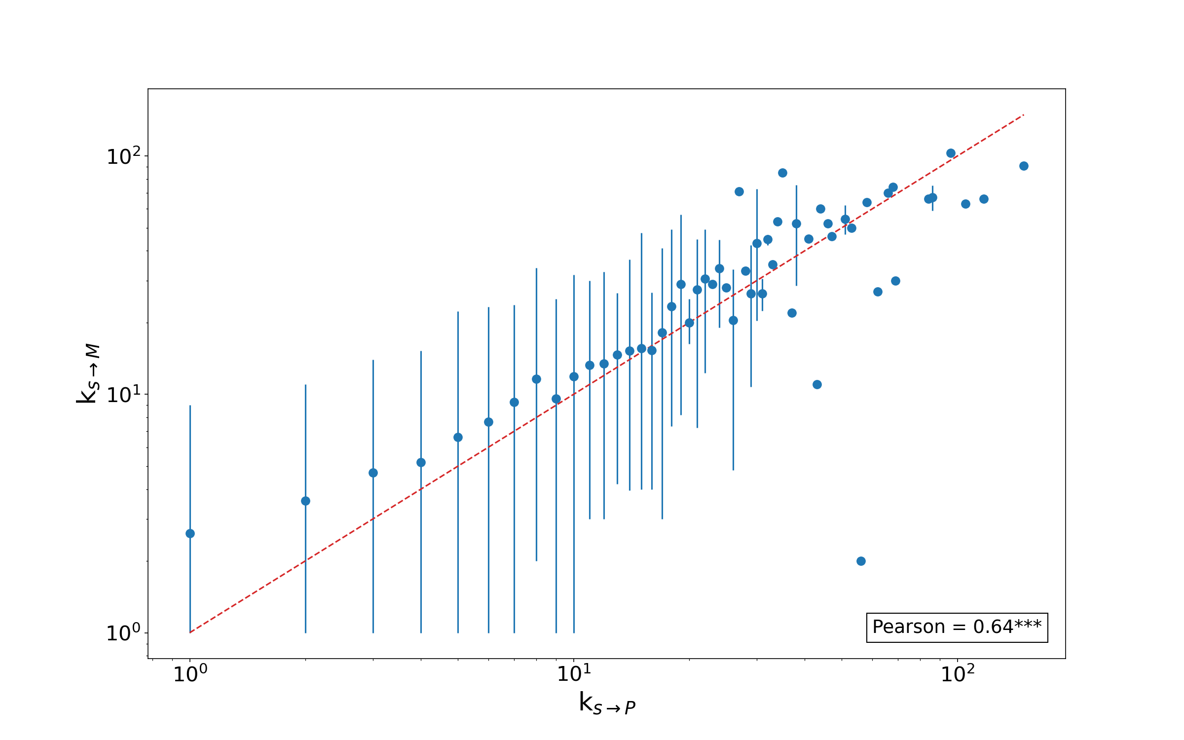
Figure 3: $k_{s\rightarrow\mathcal{M}}$ values are positively correlated with $k_{s\rightarrow\mathcal{P}}$ values (the Pearson correlation coefficient reads $r\simeq 0.64$ with a p-value smaller than 0.001), an evidence indicating that ‘generalist’ suppliers tend to be connected with a large number of manufacturers; still, many suppliers providing few products while being connected with a relatively large number of manufacturers exist. Each dot represents the average of the number of customers of the suppliers that have a particular diversification; the bars accompanying them represent the $95\%$ sample CIs.

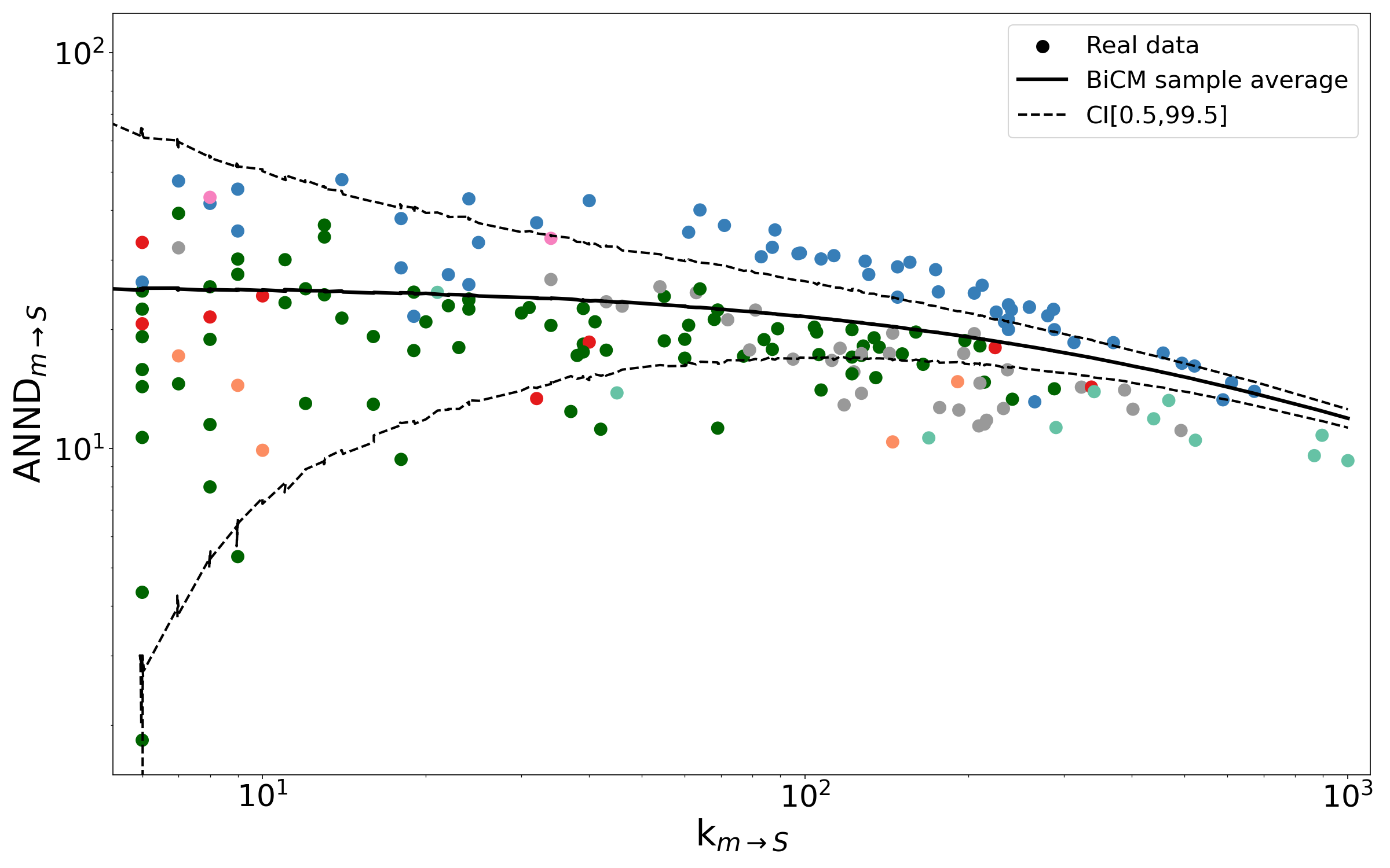
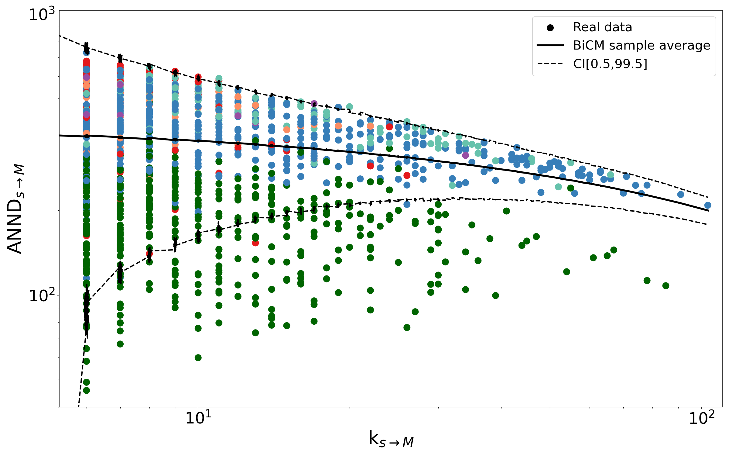
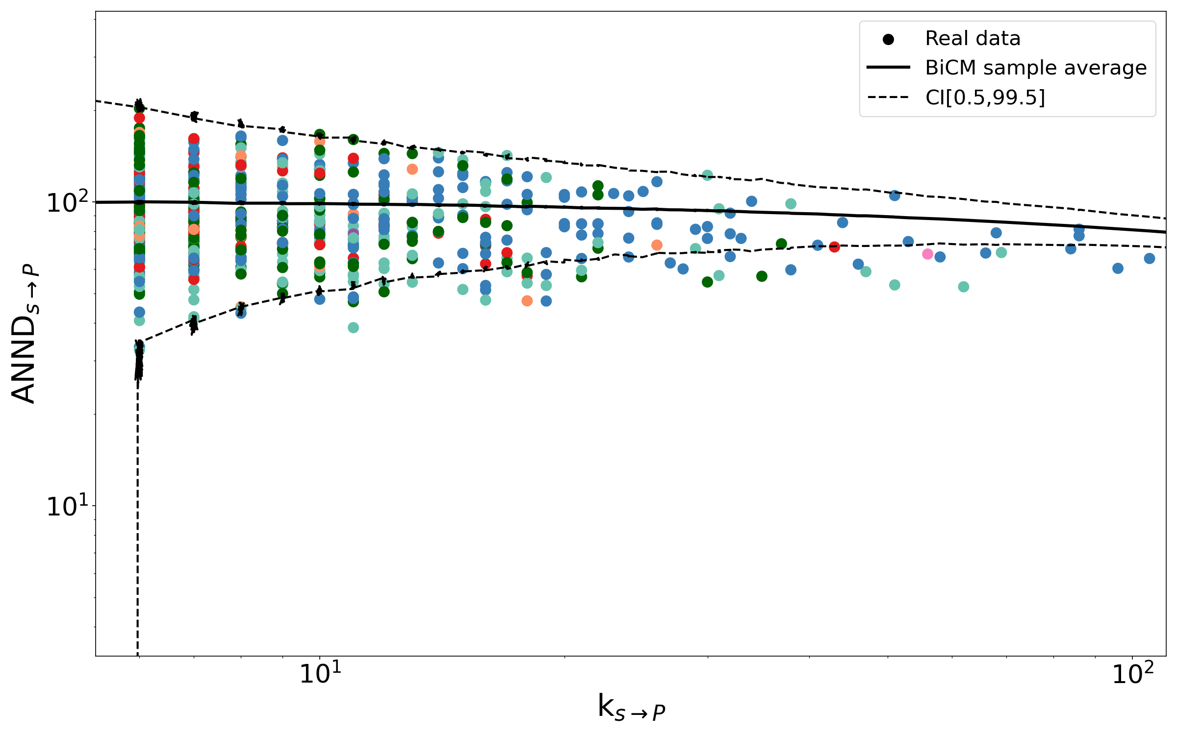
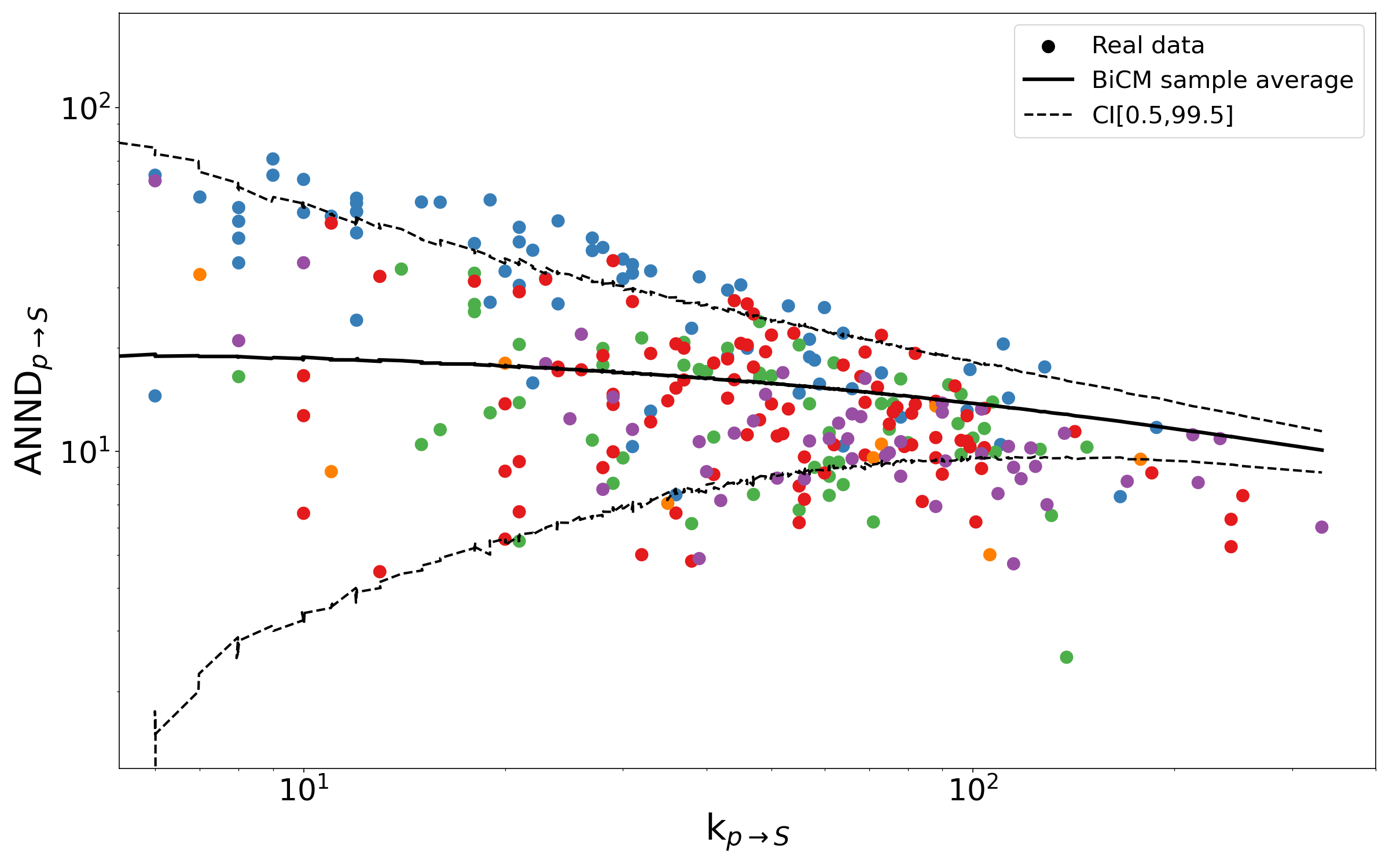
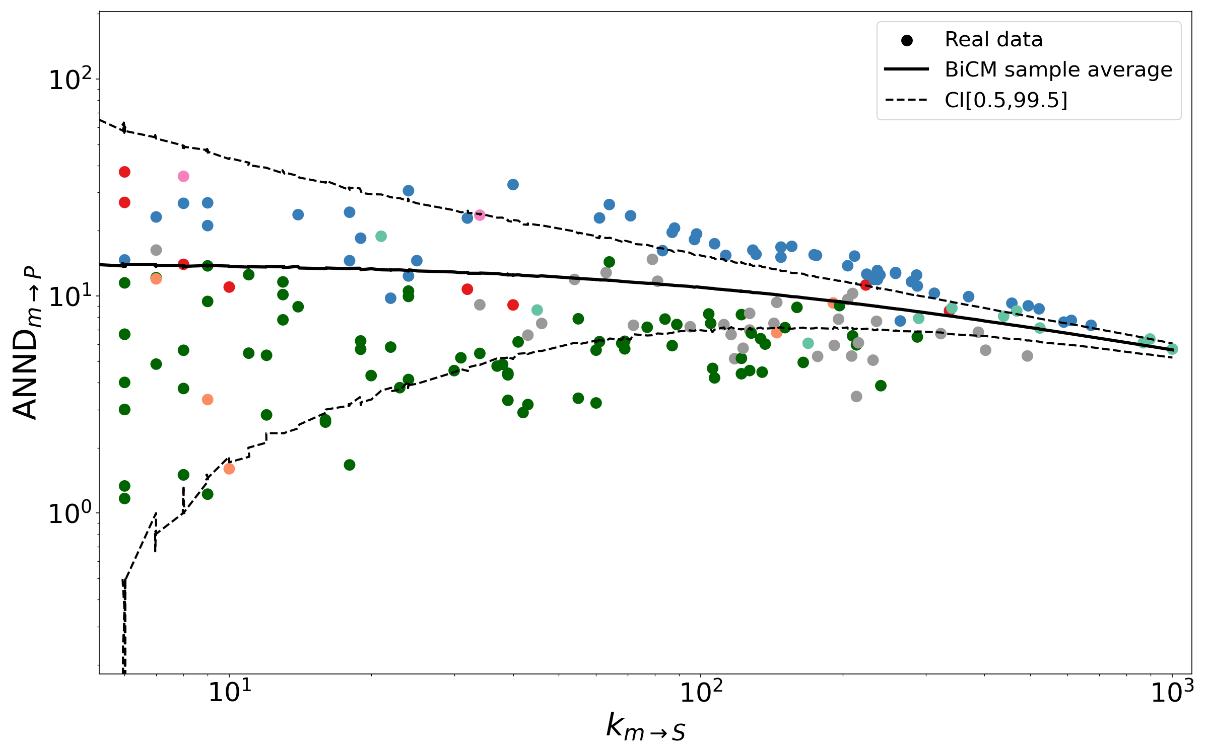
Figure 4: Top panels: $\text{ANND}_{m\rightarrow\mathcal{S}}$ scattered versus $k_{m\rightarrow\mathcal{S}}$ (left) and $\text{ANND}_{s\rightarrow\mathcal{M}}$ scattered versus $k_{s\rightarrow\mathcal{M}}$ (right). Both trends are slightly decreasing, hinting at a disassortative behavior, i.e. manufacturers (suppliers) having a large degree are generally connected with suppliers (manufacturers) having a small degree and viceversa. In other words, our results depict the automotive industry as an ecosystem populated by 1) suppliers that serve ‘bigger players’ by providing them with few products and 2) suppliers that serve a larger number of clients by providing them with a larger basket of products. Middle panels: $\text{ANND}_{s\rightarrow\mathcal{P}}$ scattered versus $k_{s\rightarrow\mathcal{P}}$ (left panel) and $\text{ANND}_{p\rightarrow\mathcal{S}}$ scattered versus $k_{p\rightarrow\mathcal{S}}$ (right panel). As for the manufacturer-supplier network, both trends are decreasing, pointing out a disassortative behavior, according to which suppliers providing many products tend to have exclusive products within their baskets, whereas suppliers providing few products tend to have a basket of ubiquitous products; in this case, however, no geographically-induced distinction between firms emerges. Bottom panel: $\text{ANND}_{m\rightarrow P}$ scattered versus $k_{m\rightarrow\mathcal{S}}$. The slightly decreasing trend confirms the picture provided by the figures above, i.e., Western and Japanese manufacturers with a larger degree tend to be connected with suppliers providing fewer products and viceversa. Nodes are colored according to their geographic location: $\bullet$ Africa, $\bullet$ Asean, $\bullet$ Chinese, $\bullet$ Indian, $\bullet$ Japanese, $\bullet$ Latin America, $\bullet$ Middle East, $\bullet$ Russian, $\bullet$ Western and $\bullet$ Joint Ventures. Products are colored according to their technological sector, i.e. $\bullet$ Chassis/Body, $\bullet$ Electrical, $\bullet$ Powertrain, $\bullet$ Interior/Exterior, $\bullet$ General parts.

III.1 Structural properties

Local connectivity.

Figure 2 shows the degree distributions of manufacturers, suppliers, and products. All of them are heavy-tailed and right-skewed, an evidence pointing out the large heterogeneity of nodes’ connectivity: more specifically, they all obey a power-law with exponential cutoff [86].

Overall, the above results indicate the presence of ‘generalist’ suppliers (i.e. providing many products) co-existing with ‘specialist’ suppliers (i.e. providing few products - $\simeq 51\%$ of suppliers sells only one product). Figure 3 further shows that the number of client manufacturers of a supplier and the number of different products it sells are positively correlated, indicating that ‘generalist’ suppliers tend to be connected with a large number of manufacturers. Still, many ‘specialist’ suppliers that are linked to a relatively large number of manufacturers exist; a noticeable exception is Motor Super, a Russian company that sells 56 different products to just 2 manufacturers, i.e. the Russian AvtoVaz and the American Chevrolet. Overall, $\simeq 41\%$ of suppliers is connected to only one manufacturer.

Assortativity.

In order to inspect the presence of degree correlations, we have scattered the $\text{ANND}_{m\rightarrow\mathcal{S}}$ values versus the $k_{m\rightarrow\mathcal{S}}$ values (top left panel of Figure 4) and the $\text{ANND}_{s\rightarrow\mathcal{M}}$ values versus the $k_{s\rightarrow\mathcal{M}}$ values (top right panel of Figure 4). As the plots show, both trends are slightly decreasing, pointing out the presence of disassortative patterns: in other words, manufacturers with many suppliers tend to be connected with suppliers having few customers, while manufacturers with few suppliers tend to be connected with suppliers having many customers; similarly, suppliers with many clients tend to be connected with manufacturers having few suppliers, while suppliers with few clients tend to be connected with manufacturers having many suppliers. Overall, then, the automotive industry resembles an ecosystem where suppliers serving (only) ‘bigger players’, by providing them few products - the so-called ‘specialists’ - co-exist with suppliers serving a larger number of clients, by providing them a larger basket of products - the so-called ‘generalists’.

To spot differences between firms induced by their geographic location, we have partitioned them into nine groups, i.e. African, Asean (i.e. Indonesia, Malaysia, South Korea, Thailand, and Vietnam), Chinese, Indian, Japanese, Middle Eastern (i.e. Egypt, Iran, and Turkey), Russian, Western (i.e. Australia, Europe, Israel, and US) and Joint Ventures (JVs) and colored them accordingly. Overall, the group of Western firms is quite well-distinguished from the group of Chinese firms and JVs. Among the manufacturers, Western ones display significantly large $\text{ANND}_{m\rightarrow\mathcal{S}}$ values, lying in the top $0.5\%$ of the ensemble distribution induced by the null model, while the $\text{ANND}_{m\rightarrow\mathcal{S}}$ values for JVs, Chinese and Japanese manufacturers are either in line with the predictions of the null or lie below the bottom $0.5\%$ confidence interval. For what concerns suppliers, instead, Chinese firms display significantly small $\text{ANND}_{s\rightarrow\mathcal{M}}$ values, lying in the bottom $0.5\%$ confidence interval, while the $\text{ANND}_{s\rightarrow\mathcal{M}}$ values for Western and Japanese suppliers are in line with the predictions of the null model. This result suggests the supply chains of the Western and Japanese automotive sector to be structurally different from the Chinese ones: Western and Japanese manufacturers tend to purchase products from suppliers whose degree is, on average, larger than the one of the suppliers serving Chinese manufacturers - in particular, the Japanese automotive industry revolves around few, big manufacturers purchasing products from many, low-degree suppliers.

For what concerns the supplier/product network, scattering the $\text{ANND}_{s\rightarrow\mathcal{P}}$ values versus the $k_{s\rightarrow\mathcal{P}}$ values and the $\text{ANND}_{p\rightarrow\mathcal{S}}$ values versus the $k_{p\rightarrow\mathcal{S}}$ values reveals its disassortative character, with suppliers selling many, less ubiquitous products and viceversa (middle panels of Figure 4) - a result that is reminiscent of the one concerning the export of countries within the (bipartite representation of the) international trade. While firms do not seem to be partitioned according to any geographic criterion, products belonging to the Electrical sector display the larger $\text{ANND}_{p\rightarrow S}$ values.

The aforementioned, geographical difference is recovered when scattering the tripartite assortativity coefficient of each manufacturer, defined as $\text{ANND}_{m\rightarrow\mathcal{P}}=\sum_{s=1}^{S}l_{ms}k_{s\rightarrow\mathcal{P}}/k_{m\rightarrow\mathcal{S}}$, versus its degree. As the bottom panel of Figure 4 confirms, Western and Japanese manufacturers tend to connect with suppliers providing a number of products that is larger than the one provided by the suppliers to which Chinese manufacturers and JVs tend to connect.

Motifs.

For what concerns the bipartite clustering coefficient, both panels of Figure 5 show an overall decreasing trend, signaling that manufacturers (suppliers) having a large degree are generally closing less squares than manufacturers (suppliers) having a small degree. Again, the group of Western and Japanese firms is quite well-distinguished from the group of Chinese firms and JVs, as the former ones display significantly large values of the bipartite clustering coefficient, lying in the top $0.5\%$ of the ensemble distribution induced by our null model. In other words, the presence of mesoscale structures characterizing the Western and Japanese subsets of firms cannot be simply traced back to the nodes degrees: rather, it represents a peculiar feature of these areas whose automotive industry appears as a highly interconnected ecosystem. Chinese firms, on the contrary, constitute a seemingly fragmented environment with different (sets of) manufacturers purchasing products from different (sets of) suppliers, each one serving few clients. Our results complement the ones about the presence of statistically significant functional structures within the automotive industry [66], clarifying that they come along a geographical signature. These results are robust with respect to the definition of the bipartite clustering coefficient (see Appendix B).

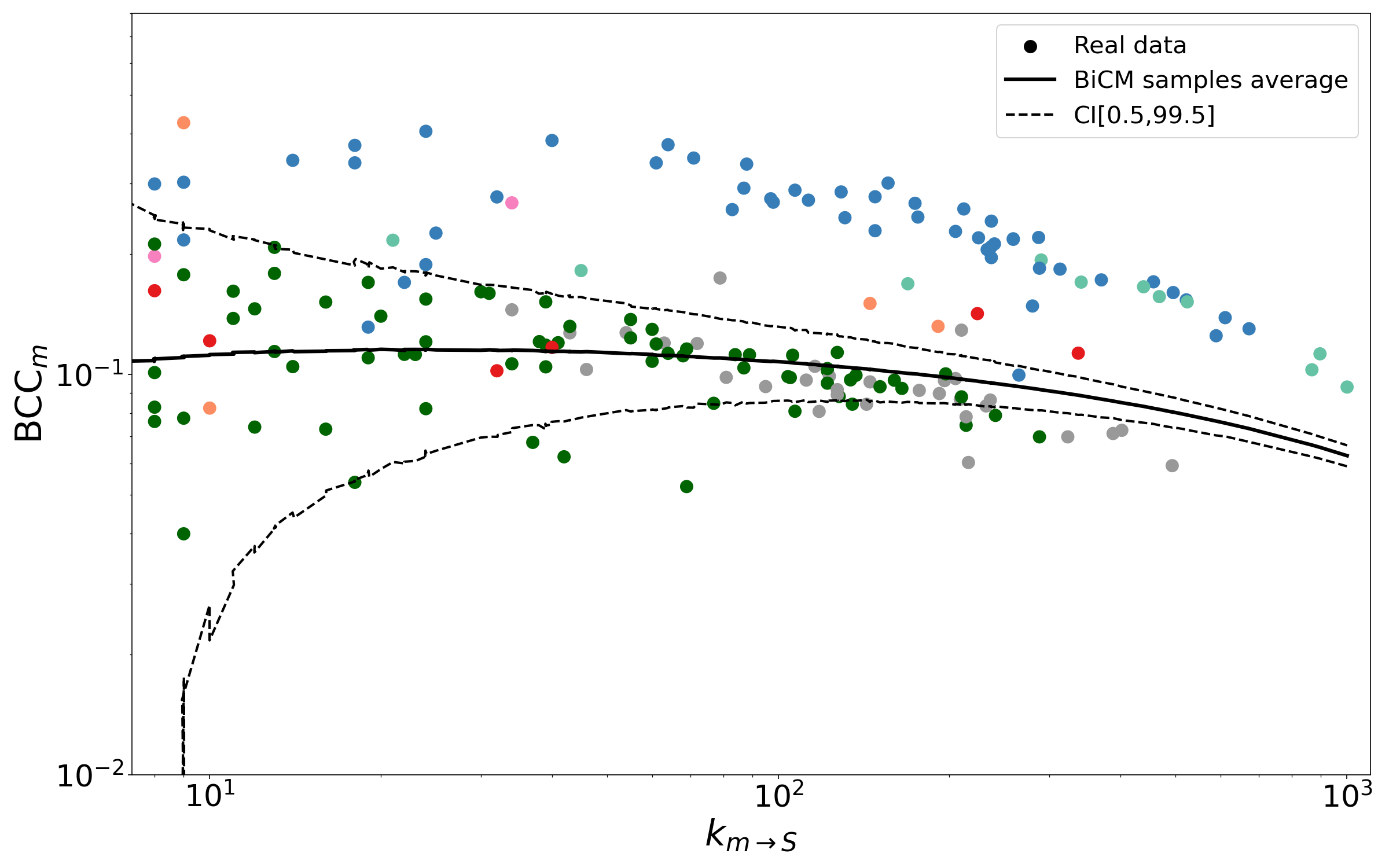
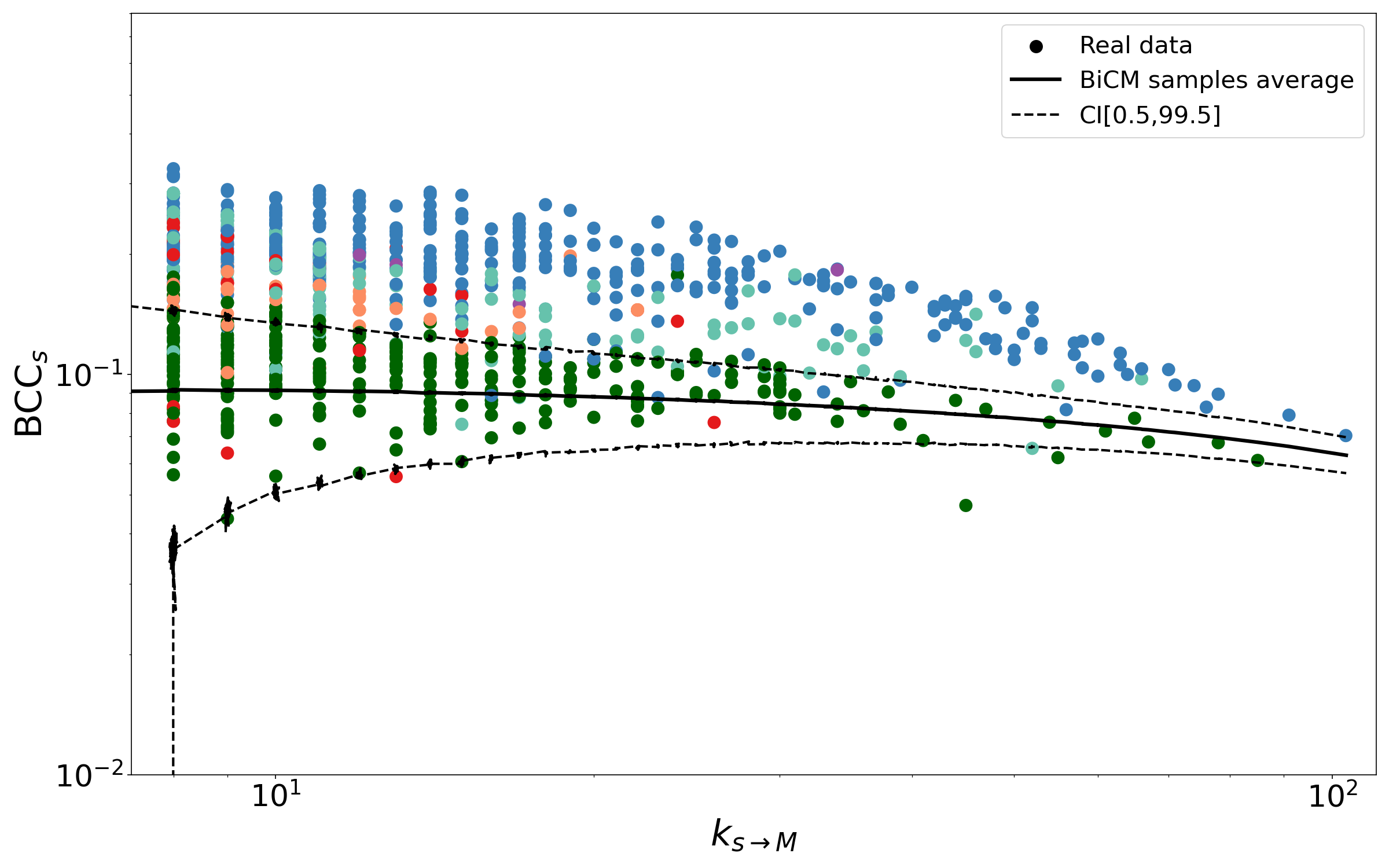
Figure 5: $\text{BCC}_{m}$ scattered versus $k_{m\rightarrow S}$ (left panel) and $\text{BCC}_{s}$ scattered versus $k_{s\rightarrow MS}$ (right panel). Both trends are overall decreasing, indicating that manufacturers (suppliers) having a large degree are generally closing less squares than manufacturers (suppliers) having a small degree. Besides, our results highlight that the automotive industry of different geographic locations is shaped by different organizing principles: while the Western ecosystem seems to be highly interconnected, where manufacturers share many suppliers that, in turn, share many different manufacturers, the Chinese ecosystem seems to be rather fragmented, with different (sets of) manufacturers purchasing products from different (sets of) suppliers, each one serving few clients. Overall, our results confirm the presence of the (statistically significant) functional structures first observed in [66], however highlighting their peculiarly geographical character. Nodes are colored according to their geographic localization: $\bullet$ Africa, $\bullet$ Asean, $\bullet$ Chinese, $\bullet$ Indian, $\bullet$ Japanese, $\bullet$ Latin America, $\bullet$ Middle East, $\bullet$ Russian, $\bullet$ Western and $\bullet$ Joint Ventures.

Subgraph centrality.

The results of the analysis of the bipartite subgraph centrality (BSC), illustrated in Figure 6, show that nodes with a larger degree tend to be more central as well. More importantly, the BSC allows us to appreciate the different behavior displayed by firms located in different countries at best: Chinese firms and JVs are, in fact, characterized by values of the BSC that are much smaller (some hardly above zero) than the values of the BSC characterizing Western and Japanese firms. Specifically, the latter (former) have a larger-than-expected (smaller-than-expected) BSC on the layer of manufacturers. Similar trends are observed when considering the layer of suppliers, the only difference being that, now, the BSC of Western and Japanese firms is, overall, in line with the predictions of the BiCM. Once again, these findings reveal Western and Japanese firms to be crossed by a large number of patterns, an evidence confirming the plethora of interconnections leading from one node to another within this portion of the network; Chinese firms, instead, seemingly belong to less interconnected, if not completely segregated, supply chains.

Suppliers’ redundancy.

Let us now complement our analysis by calculating the average suppliers’ redundancy for each manufacturer, defined as $\text{ASR}_{m}=\sum_{s=1}^{S}l_{ms}\text{RED}_{s}/k_{m\rightarrow\mathcal{S}}$ where $\text{RED}_{s}=\sum_{p=1}^{P}\sum_{s^{\prime}(\neq s)\in\mathcal{S}_{m}}r_{sp}r_{s^{\prime}p}/k_{s\rightarrow\mathcal{P}}$ and with $\mathcal{S}_{m}$ indicating the neighborhood of manufacturer $m$, i.e. the set of its suppliers. Scattering the $\text{ASR}_{m}$ values versus the $k_{m\rightarrow\mathcal{S}}$ values (see Figure 7) reveals an increasing trend, pointing out that suppliers serving manufacturers with a larger degree tend to produce a larger number of similar products; besides, the suppliers serving Western manufacturers display significantly large redundancy values, lying in the top $0.5\%$ of the ensemble distribution induced by our null model. The size of the dots is proportional to the number of countries of origin of the suppliers of each manufacturer. A clear geographical signature is present: while the suppliers serving Western and Japanese manufacturers are scattered across many different countries - e.g. 36 for Toyota and 34 for Ford - this is true to a much lesser extent for what concerns Chinese manufacturers and JVs - e.g. the number of countries hosting the suppliers of Geely and FAW Volkswagen is 10 and 15, respectively.

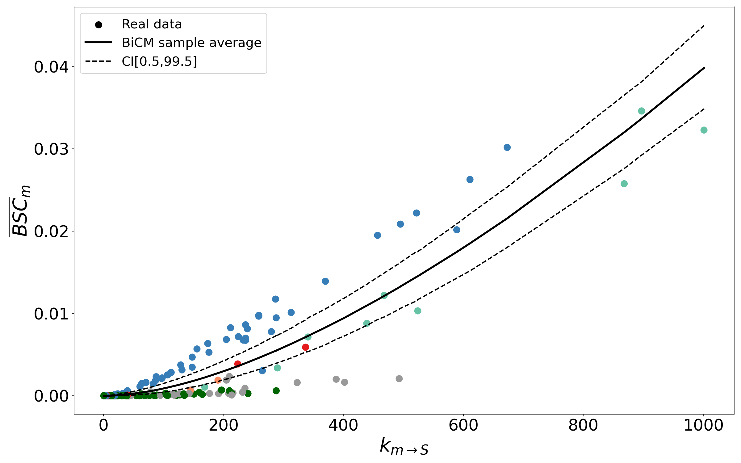
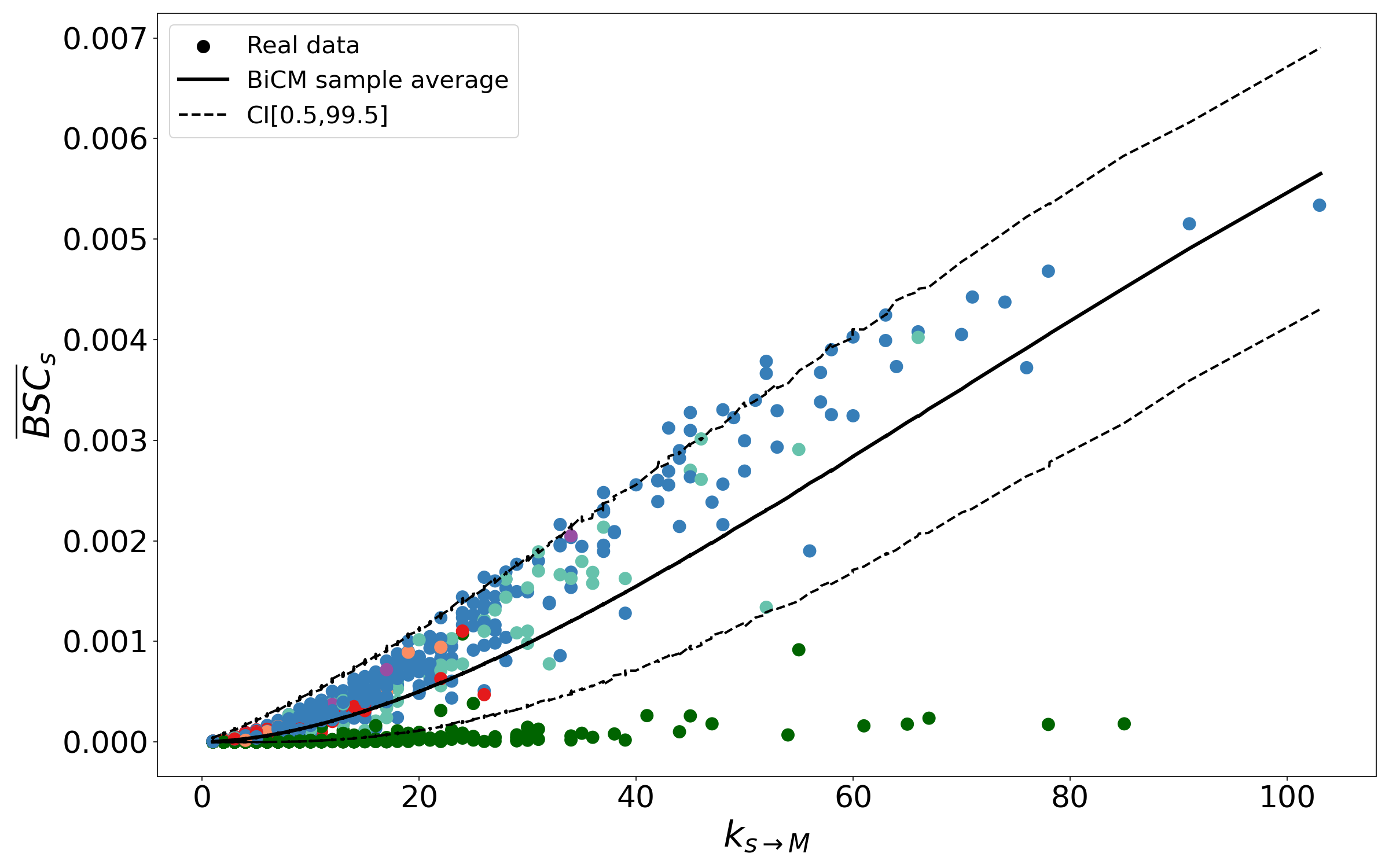
Figure 6: $\overline{\text{BSC}}_{m}$ scattered versus $k_{m\rightarrow S}$ (left panel) and $\overline{\text{BSC}}_{s}$ scattered versus $k_{s\rightarrow M}$ (right panel). Both trends are increasing, pointing out that nodes with a larger degree are also more central. Chinese firms and JVs are characterized by values of the BSC that are much smaller than those characterizing Western and Japanese firms and always smaller than expected under the BiCM, a finding seemingly confirming that Chinese firms belong to less interconnected, if not completely segregated, supply chains. Western and Japanese firms, instead, appear to be crossed by a large number of patterns - when considering the layer of manufacturers, larger-than-expected under the BiCM - an evidence confirming the plethora of interconnections leading from one node to another within this portion of the network. Nodes are colored according to their geographic localization: $\bullet$ Africa, $\bullet$ Asean, $\bullet$ Chinese, $\bullet$ Indian, $\bullet$ Japanese, $\bullet$ Latin America, $\bullet$ Middle East, $\bullet$ Russian, $\bullet$ Western and $\bullet$ Joint Ventures.

III.2 Projection of the ‘MarkLines Automotive’ dataset

Community structure of the validated projection.

Lastly, we focus on the validated projection onto each of our layers.

Figure 8 shows the validated network of manufacturers, where two manufacturers are linked if sharing a statistically significantly large number of suppliers. A markedly modular structure emerges (the value of modularity amounts at $\simeq 0.5$), the clusters of manufacturers being coherent with their geographic localization: the two, largest ones are those composed by Chinese and Western firms - which, however, are not interconnected. Instead, the Chinese cluster is linked only to the community of JVs that is constituted exclusively by Joint Ventures involving one Chinese company. The Western cluster is, in turn, connected with the cluster of JVs via the manufacturer BMW Brilliance, with the Japanese cluster via the manufacturer Nissan and with the Asean-Indian cluster via several links. Interestingly, the similarity of the two small sets of nodes (recognized by the Louvain algorithm as individual communities) which are detached from the Chinese and Western clusters is not only due to geographic proximity but also to their technological characterization: the three nodes lying on the left of the Chinese cluster (i.e. GAC Aion, Weltmeister and Xpeng) are all manufacturers of electric cars, while the four nodes lying below the Western cluster (i.e. Alpina, Lotus, McLaren and SRT) are all manufacturers of sports cars. As a last comment, let us stress once more that the Western cluster is much more internally-connected than the Chinese one, a finding further confirming that the closure of motifs, within the automotive industry, is strongly driven by geographic proximity.

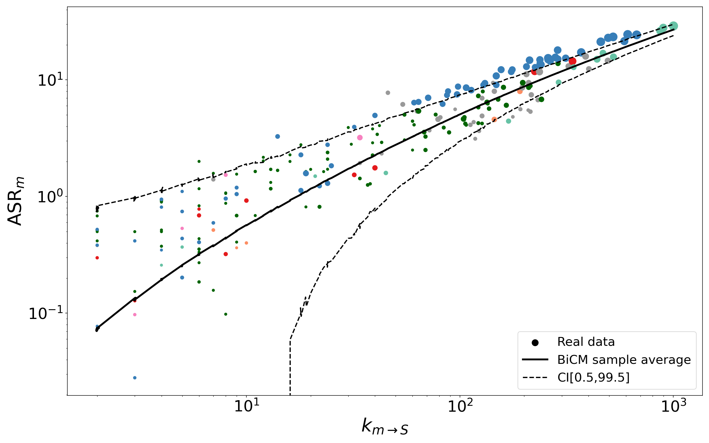
Figure 7: $\text{ASR}_{m}$ scattered versus $k_{m\rightarrow S}$. The increasing trend signals that suppliers serving manufacturers with a larger degree tend to produce a larger number of similar products. The suppliers serving Western manufacturers display the larger redundancy values; the size of dots, proportional to the number of countries of origin of the suppliers of each manufacturer, highlight a geographical signature: the suppliers serving Western and Japanese manufacturers are scattered across many, different countries (36 for Toyota and 34 for Ford) while this is true to a much lesser extent for what concerns the suppliers serving Chinese manufacturers and JVs (the number of countries hosting the suppliers of Geely and FAW Volkswagen are 10 and 15, respectively). Nodes are colored according to their geographic localization: $\bullet$ Africa, $\bullet$ Asean, $\bullet$ Chinese, $\bullet$ Indian, $\bullet$ Japanese, $\bullet$ Latin America, $\bullet$ Middle East, $\bullet$ Russian, $\bullet$ Western and $\bullet$ Joint Ventures.

As Figure 9 shows, the validated projection of suppliers (where two suppliers are linked if sharing a significantly large number of manufacturers, see Appendix C for details on how this projection was obtained) is markedly modular as well (the value of modularity amounts at $\simeq 0.6$) with clusters embodying geographic information. As evident upon inspecting the figure, the Chinese cluster is not only isolated but also (internally) fragmented, being constituted by a plethora of smaller connected components; the Indian cluster is disconnected from the rest of the network as well, although its density is quite large. The largest components are constituted by two pairs of interconnected communities, i.e. the one gathering Asean and Japanese firms and the one gathering American and European firms; German suppliers give origin to a smaller community, lying on the right of the European subgraph.

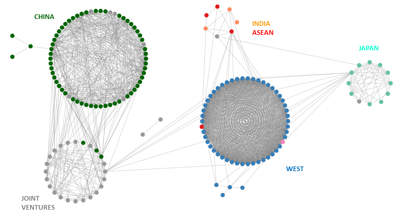
Figure 8: Validated projection of manufacturers, linked if sharing a significantly large number of suppliers. Analyzing the presence of connections between communities reveals that the Chinese cluster is solely linked to the cluster of JVs which, in turn, is connected with the Western cluster via the manufacturer BMW Brilliance; as the latter is connected with the Japanese and Asean-Indian clusters as well, it is also the most central one of our validated projection. Lastly, let us stress once more that the Western cluster is much more internally connected than the Chinese one, a finding further confirming the closure of motifs to be strongly driven by geographic proximity. Nodes are colored according to their geographic localization: $\bullet$ Africa, $\bullet$ Asean, $\bullet$ Chinese, $\bullet$ Indian, $\bullet$ Japanese, $\bullet$ Latin America, $\bullet$ Middle East, $\bullet$ Russian, $\bullet$ Western and $\bullet$ Joint Ventures.

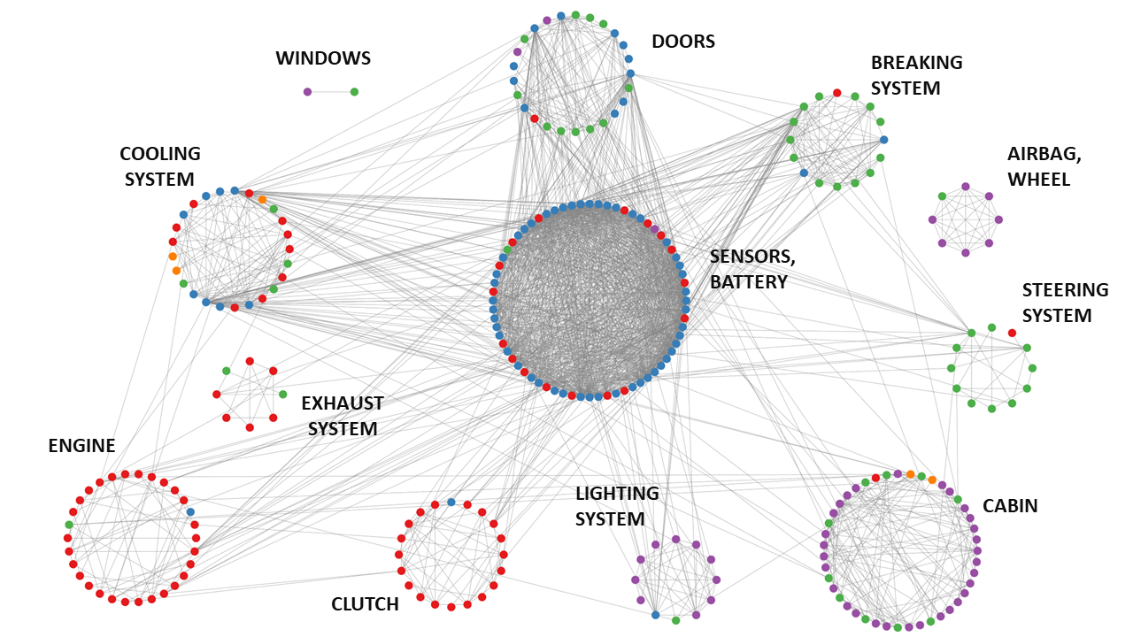
Figure 10: Validated projection of products, linked if sharing a significantly large number of suppliers. The network displays a clearly defined community structure whose clusters represent the different ‘functional modules’ that are present in a car. Nodes are colored according to their technological sector, i.e. $\bullet$ Chassis/Body, $\bullet$ Electrical, $\bullet$ Powertrain, $\bullet$ Interior/Exterior, $\bullet$ General parts.

For what concerns the supplier/product network, the validated projection of products (linked if sharing a significantly large number of suppliers) is shown in figure 10: it displays an interesting community structure (the value of modularity amounts at $\simeq 0.45$), characterized by the emergence of clusters that do not overlap with the (technological) taxonomy provided by the platform https://www.marklines.com; rather, they represent the different ‘functional modules’ that are present in a car - the list of products per community is provided in table 2 (Appendix D) - an evidence suggesting that suppliers tend to focus their production on ‘coherent’ sets of products [87, 88].

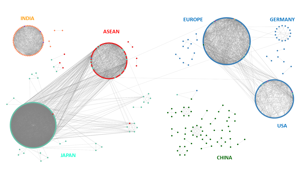
Figure 9: Validated projection of suppliers, linked if sharing a significantly large number of manufacturers. Analyzing the presence of connections between communities reveals that the Chinese cluster is isolated and internally fragmented. The largest components are constituted by two pairs of interconnected communities, formed by Asean and Japanese firms and American and European firms. Nodes are colored according to their geographic localization: $\bullet$ Africa, $\bullet$ Asean, $\bullet$ Chinese, $\bullet$ Indian, $\bullet$ Japanese, $\bullet$ Latin America, $\bullet$ Middle East, $\bullet$ Russian, $\bullet$ Western and $\bullet$ Joint Ventures.

IV Conclusions

The recent pandemic has fostered research on the structure of global supply chains [18, 22]. The use of tools routinely employed in economics [89] has allowed scholars to discuss a number of relevant economic and geopolitical issues, such as the consequences of different, national development strategies on the global value-chain of low-carbon technologies [90], the effects of the US-China trade war [91], and so on. Yet this empirical evidence is typically discussed from a qualitative or merely statistical point of view. The aim of the present paper is to bridge this gap, carrying out a quantitative and disaggregated investigation of the global structure of a specific industry, by employing methods rooted in network theory and statistical physics. Our analysis of the ‘MarkLines Automotive’ dataset allows us to draw a number of conclusions:

• Degree distributions are heavy-tailed, hence describing an ecosystem where nodes are characterized by a highly heterogeneous number of neighbors. More explicitly, ‘generalist’ suppliers selling many products co-exist together with ‘specialist’ suppliers selling few products; besides, ‘generalist’ suppliers tend to be connected with a large number of small-degree manufacturers while ‘specialist’ suppliers tend to be connected with a small number of large-degree manufacturers. Specifically, the suppliers selling only one product (amounting to $\simeq 51\%$ of the total) are connected with a subset of 166 manufacturers whose average degree amounts at $\simeq 151$, i.e. almost twice the manufacturers’ average degree - a result indicating that well-connected manufacturers are preferentially connected with suppliers seemingly providing ‘exclusive’ services.

• The analysis of the bipartite subgraph centrality points out that both manufacturers and suppliers with a larger degree tend to be more central, although the abundance of squares shows a decreasing trend when plotted as a function of the degree. These two quantities provide the neatest, geography-based partition of our basket of firms, separating Chinese from Western ones: the former close a smaller number of squares than the latter, hence providing an indication that the Chinese ecosystem is less integrated than the Western one. This is particularly evident when considering the set of Chinese suppliers: the limited, although statistically significant, number of neighbours shared by them induces a projection that is made of several, disconnected components. Although this may be (at least, partly) induced by the peculiar way this projection has been obtained, our conclusions are supported by the methodologically different analysis of of [92], which finds that the Chinese automotive industry is characterized by a large degree of internal fragmentation, which is in play even at a territorial level, as several components correspond to different Chinese provinces.

• The information provided by redundancy complements the one provided by geography, clarifying that the presence of (many) suppliers providing the same products to a manufacturer is compatible with a broader geographical distribution of the manufacturer’s plants. By converse, the presence of (fewer) suppliers selling different products to a manufacturer is compatible with a narrower geographical distribution of the manufacturer’s plants - in certain cases, a very local one. This result also suggests the manufacturers belonging to the first group are more resilient than the ones belonging to the second group, as their production is apparently less prone to interruptions due to supply shortages.

• Projecting on the layer of manufacturers reveals that the Chinese cluster is solely connected with the cluster of Chinese JVs, a result indicating that Chinese manufacturers do not share (a significantly large number of) suppliers with other manufacturers. Again, this is supported [92], who observe that the Chinese government adopted protectionist policies to boost the development of an indigenous automotive industry, forcing Chinese JVs to buy the $40\%-80\%$ of their components from Chinese suppliers.

• Taken together, our results confirm the prominent role played by square patterns in shaping the structure of interfirm networks [66]. In our case, this becomes evident when considering how the network projections are obtained, i.e. upon linking any two nodes, say $m$ and $m^{\prime}$, in case the number of neighbors they have in common is found to be significantly large. As this number coincides with the number of shared V-motifs $V_{mm^{\prime}}$ which, in turn, is related to the number of X-motifs via the relationship $X_{mm^{\prime}}=V_{mm^{\prime}}(V_{mm^{\prime}}-1)/2$, our validation procedure provides (an, at least, indirect) information about which pairs of nodes are likely to share a significantly large number of square motifs as well.

As a last remark, we would like to stress that the investigation of the economic, historical, and social motivations at the origin of the geographic-related structures we found is beyond the scope of the present paper. Here, we have shown that the adoption of tools from complex networks theory can lead to the discovery of clear, structural features shaping international supply chains (in this case, concerning the automotive sector) that should not be overlooked during the model-building phase: these patterns, in fact, could inform methods for reconstructing production networks [93] - which aim at overcoming the limitations affecting available datasets by adopting statistically-grounded techniques [62], machine learning tools [55, 94, 95, 57] or proper data proxies [96] - to be later employed for stress testing [41, 97, 40].

V Appendix A.
Data cleaning and harmonization

Here we detail the procedure used to clean and harmonize the ‘MarkLines Automotive’ dataset.

First, we dealt with the presence of companies, reported along with their divisions, with multiple names that do not necessarily correspond to the actual taxonomy of the firm (e.g. ‘BAIC Motor’ appears as ‘BAIC’, ‘BAIC Motor’ and ‘BAIC Group Off-road Vehicles’). Name homogenization was carried out by reconstructing the actual taxonomy of each group. Specifically, the corrections introduced are listed below:

• the instances of ‘BAIC’ with Senova and Beijing models, ‘BAIC Motor’ and ‘BAIC Group Off-road Vehicles’ were listed as ‘BAIC Motor’;

• the instances of ‘BAIC’ with Weiwang models were listed as ‘BAIC Yinxiang’;

• ‘Changan’, ‘Chongqing Changan’ and ‘Changan Commercial Vehicles’ were listed as ‘Chongqing Changan’;

• ‘Dongfeng’, ‘Dongfeng Motor’ and ‘Dongfeng Passenger Vehicles’ were listed as ‘Dongfeng Motor’;

• the instances of ‘FAW’, ‘FAW Car’ with Bestune models and ‘FAW Bestune’ were listed as ‘FAW Bestune’;

• the instances of ‘FAW’, ‘FAW Haima’ and ‘FAW Car’ with Haima models were listed as ‘FAW Haima’;

• the instances of ‘FAW’, ‘FAW Hongqi’ and ‘FAW Car’ with Hongqi models were listed as ‘FAW Hongqi’;

• ‘GAC Aion’ and ‘GAC NE’ were listed as ‘GAC Aion’;

• the instances of ‘GAC’ with Leopaard models and ‘GAC Changfeng’ were listed as ‘GAC Changfeng’;

• the instances of ‘GAC Motor’, ‘Trumpchi’ and ‘GAC’ with Trumpchi models were listed as ‘GAC Motor’;

• the instances of ‘Jiangling Holdings’, ‘JMH’ and ‘Jiangling’ with Landwind models were listed as ‘JMH’;

• ‘Jiangling Motors’ and ‘JMC’ were listed as ‘JMC’;

• the instances of ‘SAIC Maxus’, ‘SAIC’ and ‘SAIC Motors’ with Maxus models were listed as ‘SAIC Maxus’;

• the instances of ‘SAIC MG’, ‘MG’, ‘MG Motors’, ‘SAIC’ and ‘SAIC Motors’ with MG models were listed as ‘SAIC MG’;

• the instances of ‘SAIC Roewe’, ‘SAIC’ and ‘SAIC Motors’ with Roewe models were listed as ‘SAIC Roewe’.

Second, we addressed the simultaneous presence of both parent companies and their divisions as manufacturers of the same models (e.g. ‘Daimler Group’ along with ‘Mercedes-Benz’ and ‘Smart’, ‘GM’ along with ‘Chevrolet’ and ‘Cadillac’, etc.); in order to remove such ambiguity, we decided to split the parent companies into their divisions according to the produced models:

• ‘Daimler’ was split into ‘Bharat Benz’, ‘Mercedes-Benz’, ‘Mercedes-AMG’, ‘Smart’;

• ‘Fiat Chrysler’ was split into ‘Abarth’, ‘Alfa Romeo’, ‘Chrysler’, ‘Dodge’, ‘Fiat’, ‘Jeep’, ‘Lancia’, ‘Ram’ and ‘SRT’;

• ‘Ford’ was split into ‘Ford’ and ‘Lincoln’;

• ‘GM’ was split into ‘Buick’, ‘Cadillac’, ‘Chevrolet’, ‘Pontiac’, ‘Opel’ and ‘Opel/Vauxhall’;

• ‘Jaguar Land Rover’ was split into ‘Jaguar’ and ‘Land Rover’.

Third, we merged pairs of manufacturers in case one of them produced only vehicle models also produced by the other one. This led to the following mergers:

• ‘Brilliance Jinbei’ with ‘Renault Brilliance Jinbei’;

• ‘Brilliance Xinyuan’ with ‘Brilliance Shineray’;

• ‘Chengdu Xindadi’ with ‘Shanghai Maple’ and ‘Geely’;

• ‘Dongfeng Venucia’ with ‘Dongfeng Nissan’;

• ‘FAW Xiali’ with ‘Tianjin FAW Xiali’;

• ‘Guangqi Honda’ with ‘GAC Honda’;

• ‘Reva’ with ‘Mahindra Reva’;

• ‘Rongcheng Huatai’ with ‘Hawtai’;

• ‘Weltmeister’ with ‘WM Motors’;

• ‘Jiangxi Changhe Suzuki’ and ‘Zhicheng Automobile’ with ‘Changhe Suzuki’.

Finally, we merged the following manufacturers as they represent different plants of the same company:

• ‘FAW Toyota’, ‘Tianjin FAW Toyota’, ‘SFTM’ and ‘SFTM Changchun Fengyue’;

• ‘SAIC GM’, ‘SAIC GM Dong Yue’ and ‘SAIC GM Norsom’.

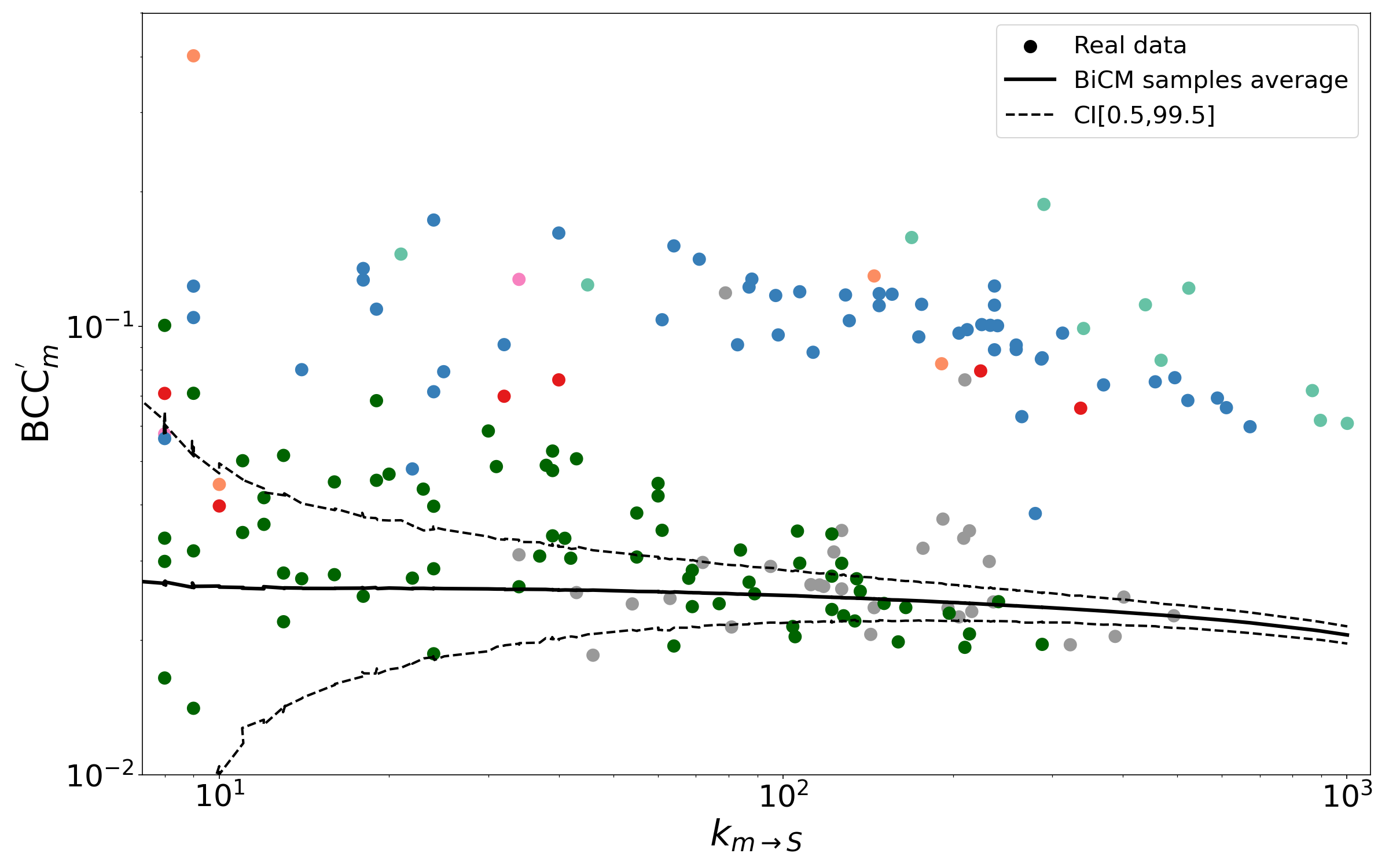
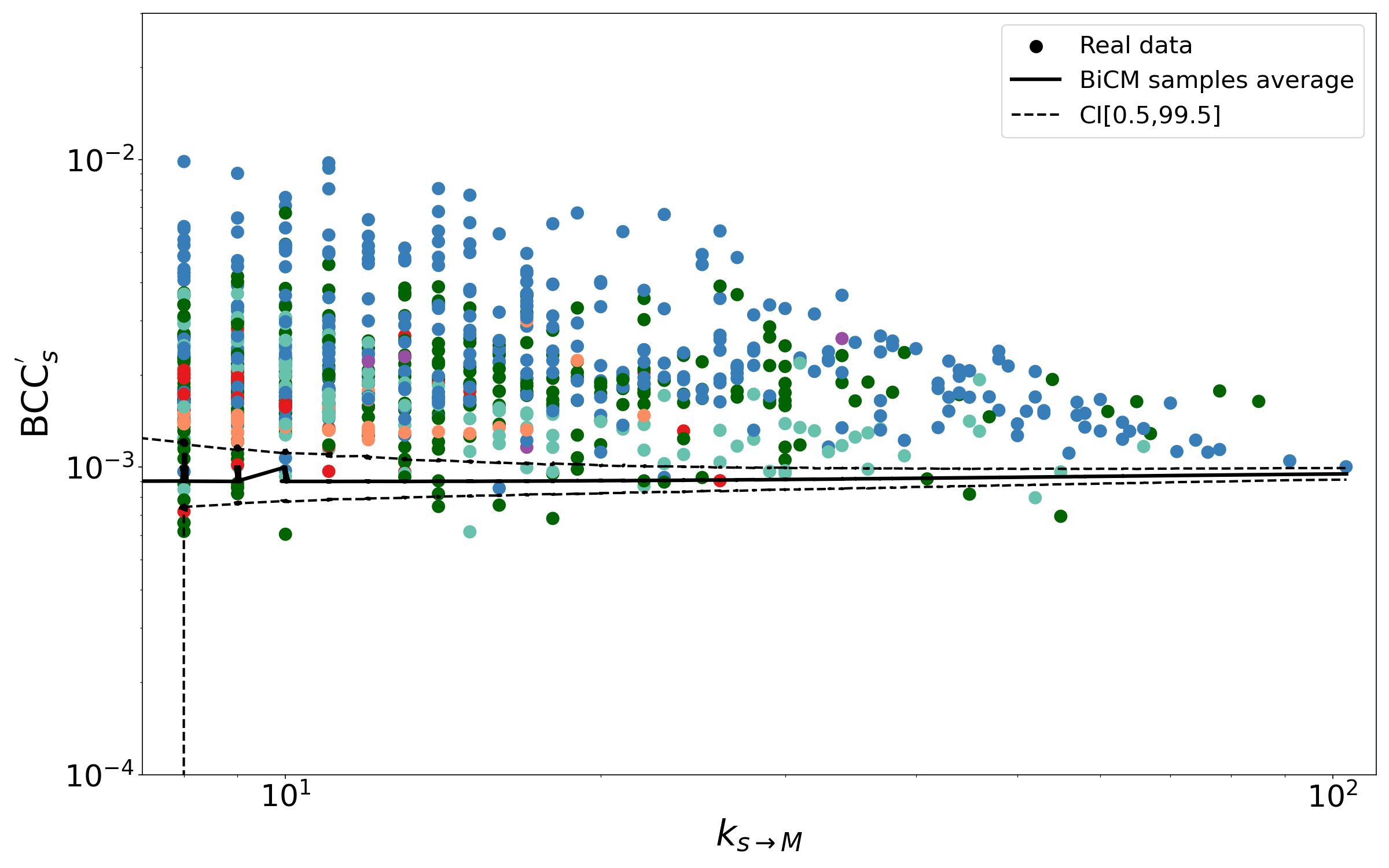
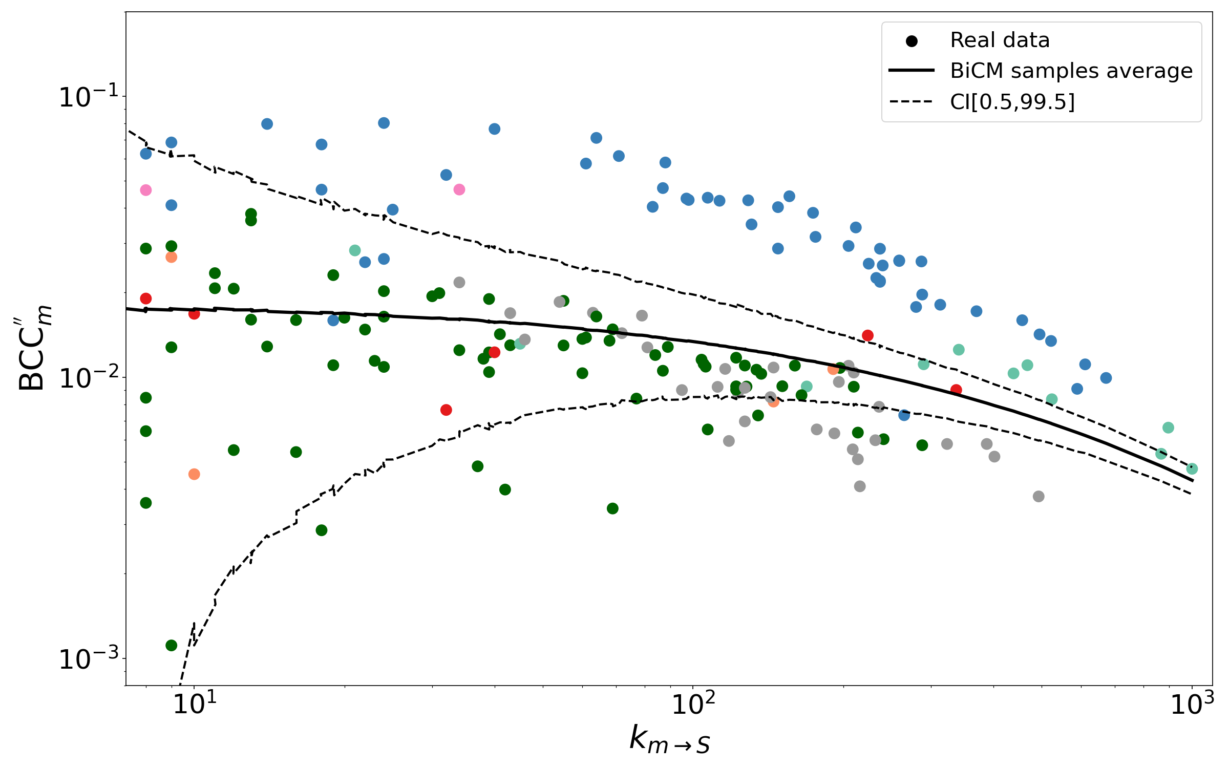
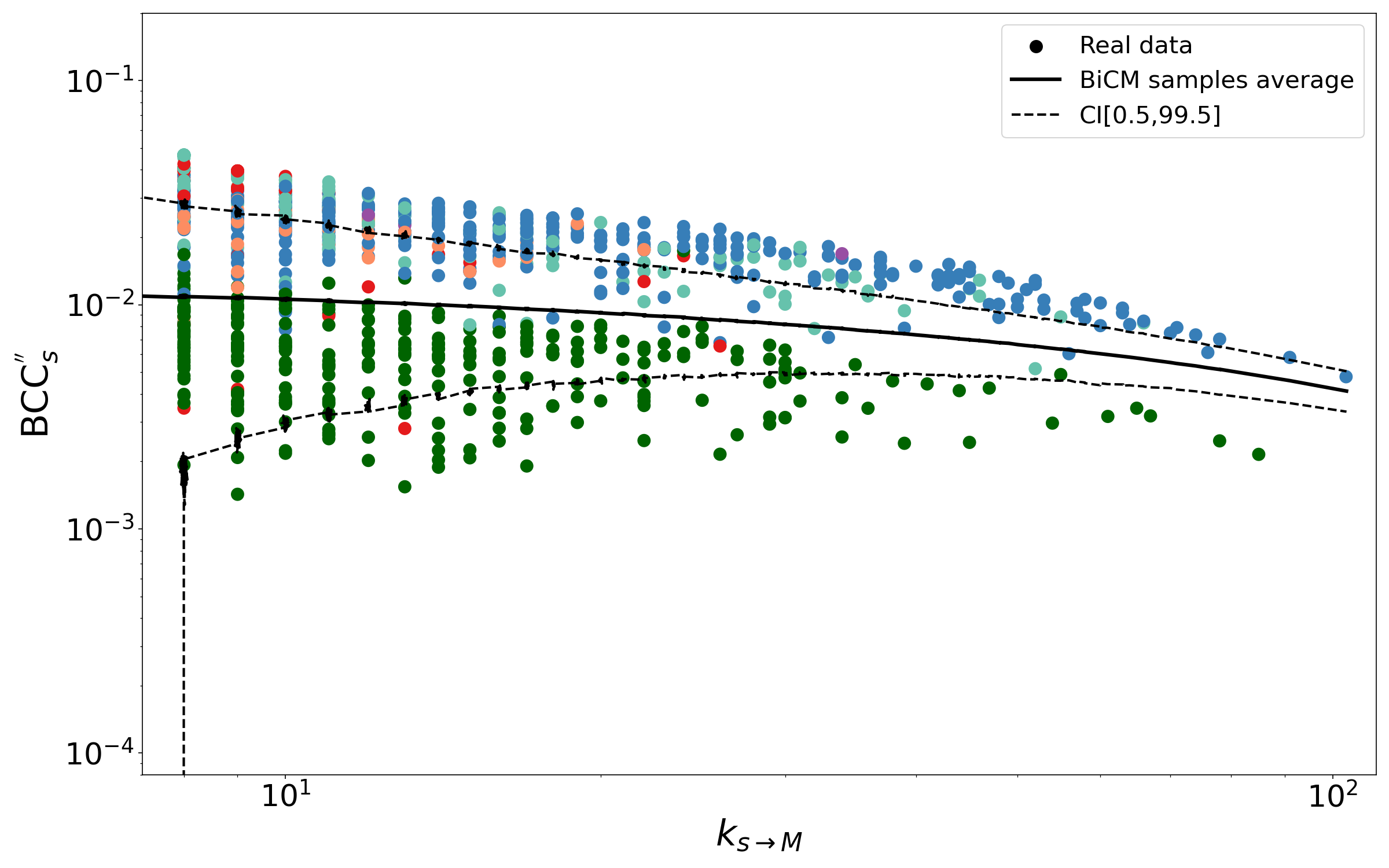
Figure 11: Bipartite clustering coefficient (top panels: (15); bottom panels: (16)) scattered versus the degree of manufacturers (left panels) and suppliers (right panels). All trends are overall decreasing, confirming that manufacturers (suppliers) having a large degree are generally closing less squares than manufacturers (suppliers) having a small degree. Again, Western and Japanese firms are clearly distinguished from Chinese firms and JVs on both layers - with definition (16) providing the neatest separation: while the clustering coefficient of the former is over-represented on both layers, the clustering coefficient of the latter is either in line with the predictions of the BiCM or under-represented. Nodes are colored according to their geographic localization: $\bullet$ Africa, $\bullet$ Asean, $\bullet$ Chinese, $\bullet$ Indian, $\bullet$ Japanese, $\bullet$ Latin America, $\bullet$ Middle East, $\bullet$ Russian, $\bullet$ Western and $\bullet$ Joint Ventures.

VI Appendix B.
Bipartite clustering coefficient: alternative definitions

Let us, now, consider two, alternative formulations of the bipartite clustering coefficient. The definition provided in [98] reads

$$\text{BCC}_{m}^{{}^{\prime}}=\frac{\sum_{s<s^{\prime}}q_{m}(s,s^{\prime})}{\sum_{s<s^{\prime}}[(u_{s}-\eta_{m}(s,s^{\prime}))(u_{s^{\prime}}-\eta_{m}(s,s^{\prime}))+q_{m}(s,s^{\prime})]}$$ (15)

where $\eta_{m}(s,s^{\prime})=1+q_{m}(s,s^{\prime})$. According to this definition, the total number of closed squares involving manufacturer $m$ is given by the product of degrees of all pairs of its neighbours, excluding the number of squares that are already closed. Otherwise stated, the total number of closed squares coincides with the number of possible ‘matchings’, achievable by rewiring existing links, between the neighbors of $s$ and those of $s^{\prime}$.

A third, possible definition reads

$$\text{BCC}_{m}^{{}^{\prime\prime}}=\frac{\sum_{s<s^{\prime}}q_{m}(s,s^{\prime})}{(M-1)d_{m}(d_{m}-1)/2};$$ (16)

according to it, the total number of closed squares involving manufacturer $m$ coincides with the number of squares that could become closed upon connecting, by adding new links, all pairs of its neighbours (e.g. $s$ and $s^{\prime}$) with the same neighbour.

As shown in figure 11, the obtained trends are very similar to those illustrated in figure 5.

 

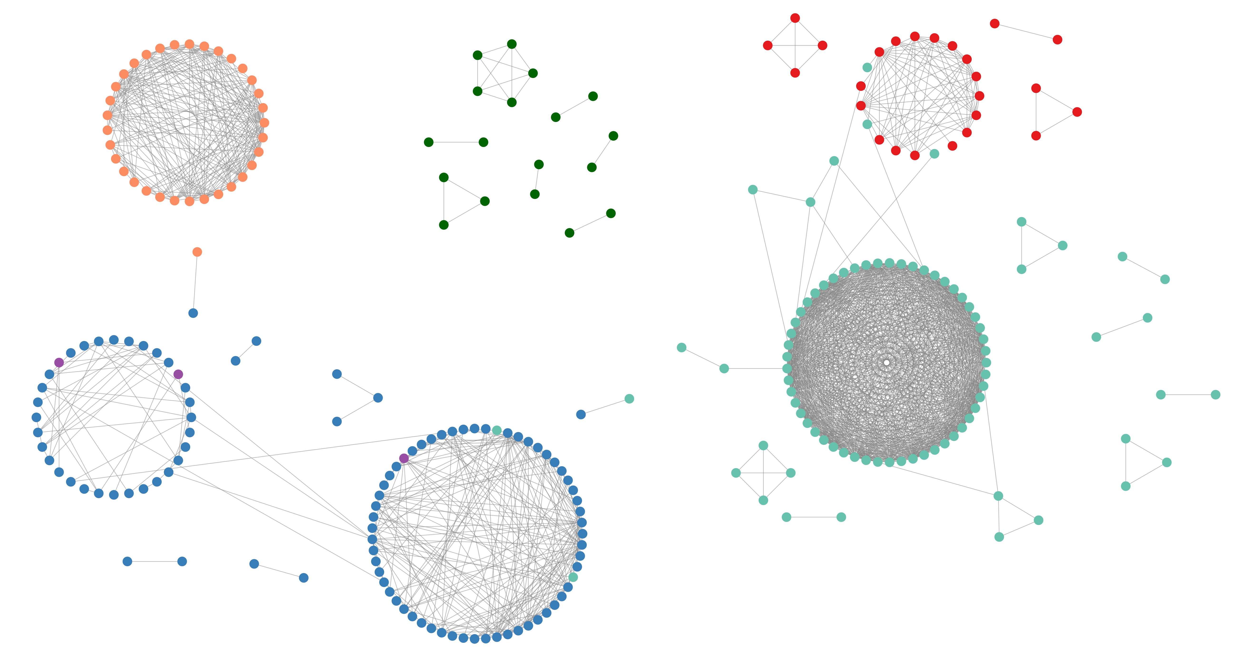
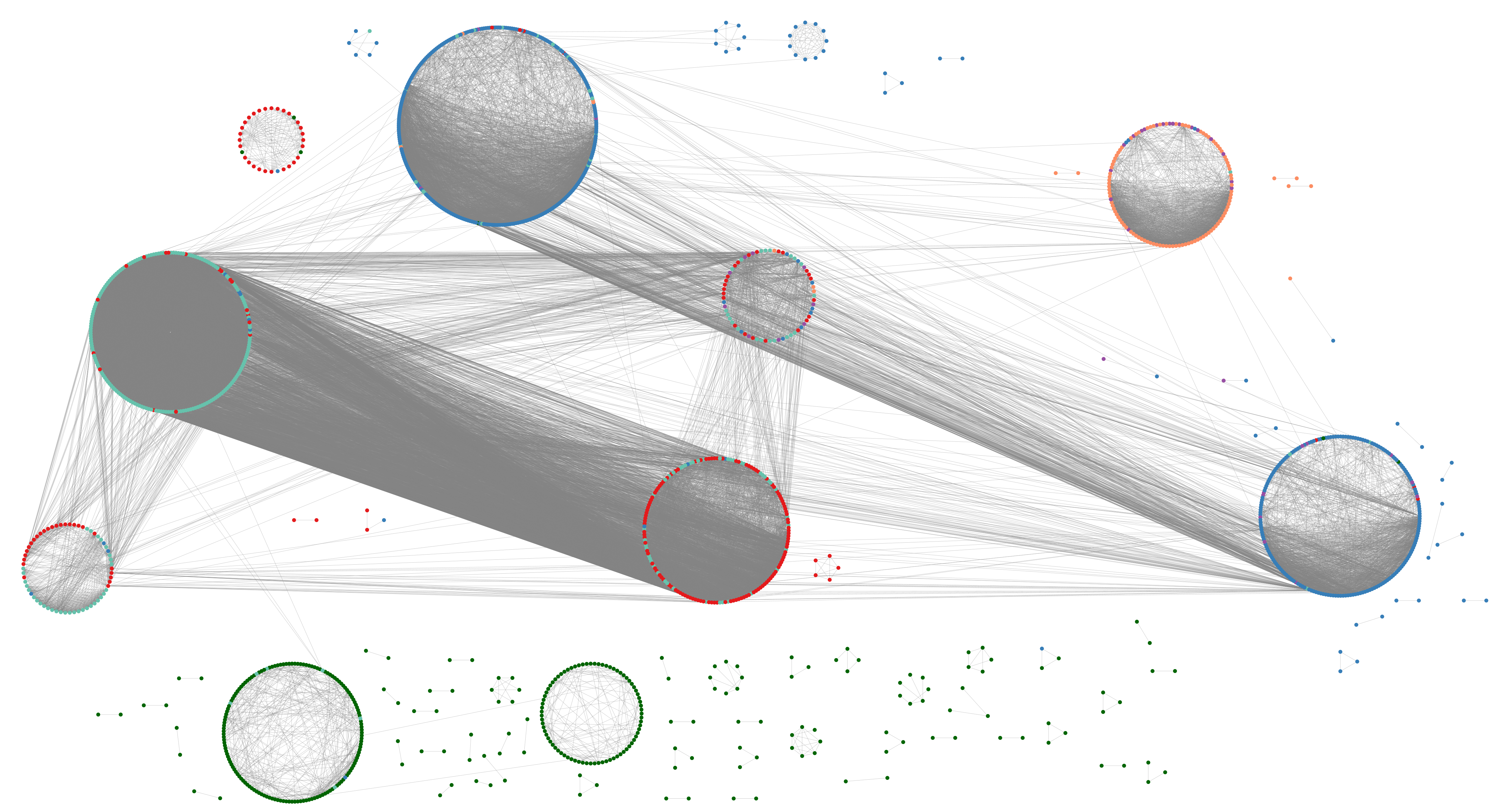
Figure 12: Validated projections of suppliers, obtained upon choosing the threshold values $t=10^{-5}$ (top panel) and $t=10^{-3}$ (bottom panel). The two projections both display similar features with respect to the one obtained with a threshold of $t=10^{-4}$ (see fig.9), such as the fragmentation of Chinese suppliers into several small connected components, the isolation of the Indian cluster, etc. Nodes are colored according to their geographic localization: $\bullet$ Africa, $\bullet$ Asean, $\bullet$ Chinese, $\bullet$ Indian, $\bullet$ Japanese, $\bullet$ Latin America, $\bullet$ Middle East, $\bullet$ Russian, $\bullet$ Western.

VII Appendix C.
Choosing the threshold for the validated projection of suppliers

When building the validated network of suppliers, the application of the FDR criterion as described in the main text yields an empty graph. In order to retain some information, we softened the validation procedure by neglecting the correction for testing multiple hypotheses while lowering the threshold $t$ - for the sake of robustness, we employed three, different values, i.e. $t=10^{-3}$, $t=10^{-4}$ and $t=10^{-5}$. The corresponding projections (i.e. figure 9, obtained upon choosing $t=10^{-4}$, and figure 12, obtained upon choosing $t=10^{-3}$ and $t=10^{-5}$) show comparable structural features - namely the fragmentation of Chinese suppliers into several small connected components, the isolation of the Indian cluster, the division of Western firms into one American and one European cluster, etc. - thus corroborating the validity of these findings.

VIII Appendix D.
Composition of products communities in the monopartite projection

Table 2: List of products populating the corresponding projection, together with their technological classification and the community they belong to. As stressed in the main text, the community structure we identify does not match with the (technological) taxonomy provided by the platform https://www.marklines.com; rather, it identifies the different ‘functional modules’ that are present in a car.

Product	Layer	Community
Boot	Interior/Exterior	Cooling System
Bush	Interior/Exterior	Cooling System
Bearing	Interior/Exterior	Cooling System
Fuel hose	Powertrain	Cooling System
Engine mount	Powertrain	Cooling System
Radiator	Powertrain	Cooling System
Radiator hose	Powertrain	Cooling System
Fuel line	Powertrain	Cooling System
Oil cooler	Powertrain	Cooling System
Cooling fan module	Powertrain	Cooling System
Engine bearing	Powertrain	Cooling System
Engine cooling module	Powertrain	Cooling System
Inter cooler	Powertrain	Cooling System
Power steering hose	Chassis/Body	Cooling System
Wheel bearing	Chassis/Body	Cooling System
Brake hose	Chassis/Body	Cooling System
Brake line	Chassis/Body	Cooling System
Heater hose	Electrical	Cooling System
Radiator fan controller	Electrical	Cooling System
AC HVAC	Electrical	Cooling System
Condenser	Electrical	Cooling System
AC hose	Electrical	Cooling System
Heater	Electrical	Cooling System
Air conditioner ECU	Electrical	Cooling System
AC compressor	Electrical	Cooling System
Inside door handle	General Parts	Doors
Outside door handle	General Parts	Doors
Shift lever	Powertrain	Doors
Side door closure	Chassis/Body	Doors
Convertible roof	Chassis/Body	Doors
Key cylinder steering lock	Chassis/Body	Doors
Back door/trunk lock	Chassis/Body	Doors
Door module	Chassis/Body	Doors
Window regulator	Chassis/Body	Doors
Side door lock	Chassis/Body	Doors
Wiper system	Chassis/Body	Doors
Wiper arm/blade	Chassis/Body	Doors
Hinge	Chassis/Body	Doors
Tailgate trunk closure	Chassis/Body	Doors
Lever combination switch	Electrical	Doors
Power tailgate trunk ECU	Electrical	Doors
Junction box	Electrical	Doors
Power sliding door ECU	Electrical	Doors
Horn	Electrical	Doors
Relay fuse	Electrical	Doors
Wiring harness	Electrical	Doors
Electrical connector	Electrical	Doors
Motor actuator	Electrical	Doors
Switch	Electrical	Doors
Keyless entry start system	Electrical	Doors

Product	Layer	Community
Pedestrian protection airbag	General Parts	Electronic Control Units
HVEV ECU	Powertrain	Electronic Control Units
Ignition coil	Powertrain	Electronic Control Units
Diesel injector	Powertrain	Electronic Control Units
Engine management system	Powertrain	Electronic Control Units
Battery control ECU	Powertrain	Electronic Control Units
On board charger	Powertrain	Electronic Control Units
Inverter	Powertrain	Electronic Control Units
DC DC converter	Powertrain	Electronic Control Units
Battery	Powertrain	Electronic Control Units
Fuel pump	Powertrain	Electronic Control Units
Glow plug	Powertrain	Electronic Control Units
Spark plug	Powertrain	Electronic Control Units
Starter motor	Powertrain	Electronic Control Units
Alternator generator	Powertrain	Electronic Control Units
Throttle body	Powertrain	Electronic Control Units
Fuel injector	Powertrain	Electronic Control Units
HVPHVEV battery	Powertrain	Electronic Control Units
Power steering motor	Chassis/Body	Electronic Control Units
Active engine mount ECU	Electrical	Electronic Control Units
Seatbelt ECU	Electrical	Electronic Control Units
Stop start system ECU	Electrical	Electronic Control Units
Air flow sensor	Electrical	Electronic Control Units
Lane keeping assist system ECU	Electrical	Electronic Control Units
Electronically controlled all wheel drive ECU	Electrical	Electronic Control Units
Cruise control	Electrical	Electronic Control Units
Camera ECU	Electrical	Electronic Control Units
Door ECU	Electrical	Electronic Control Units
Clearance sonar ECU	Electrical	Electronic Control Units
Head lamp ECU	Electrical	Electronic Control Units
Head lamp leveling ECU	Electrical	Electronic Control Units
Power seat ECU	Electrical	Electronic Control Units
Occupant detection system	Electrical	Electronic Control Units
Object detection ECU	Electrical	Electronic Control Units
Antitheft immobilizer	Electrical	Electronic Control Units
Power steering ECU	Electrical	Electronic Control Units
Milliwave and laser radar	Electrical	Electronic Control Units
Steering sensor	Electrical	Electronic Control Units
Onboard camera	Electrical	Electronic Control Units
Pedal sensor	Electrical	Electronic Control Units
Head up display	Electrical	Electronic Control Units
Pressure sensor	Electrical	Electronic Control Units
Temperature sensor	Electrical	Electronic Control Units
Knock sensor	Electrical	Electronic Control Units
Glowplug controller	Electrical	Electronic Control Units
Airbag sensor	Electrical	Electronic Control Units
ADAS ECU	Electrical	Electronic Control Units
Electronic control unit	Electrical	Electronic Control Units
Rain light sensor	Electrical	Electronic Control Units
Car navigation system	Electrical	Electronic Control Units
Body control ECU	Electrical	Electronic Control Units
Display	Electrical	Electronic Control Units
ABS ECU	Electrical	Electronic Control Units
Tire pressure monitoring system ECU	Electrical	Electronic Control Units
OBD interface	Electrical	Electronic Control Units
Park assist system	Electrical	Electronic Control Units
Airbag ECU	Electrical	Electronic Control Units
Oxygen sensor	Electrical	Electronic Control Units
Crank cam sensor	Electrical	Electronic Control Units
Transmission ECU	Electrical	Electronic Control Units
Electronically controlled suspension ECU	Electrical	Electronic Control Units
Antenna	Electrical	Electronic Control Units
In-vehicle infotainment	Electrical	Electronic Control Units
Speed sensor	Electrical	Electronic Control Units
Telematics	Electrical	Electronic Control Units
Meter	Electrical	Electronic Control Units
Car audio	Electrical	Electronic Control Units
Engine control unit	Electrical	Electronic Control Units

Product	Layer	Community
Seatbelt pretensioner	General Parts	Airbags, Wheel
Side airbag	General Parts	Airbags, Wheel
Driver airbag	General Parts	Airbags, Wheel
Knee airbag	General Parts	Airbags, Wheel
Passenger airbag	General Parts	Airbags, Wheel
Curtain airbag	General Parts	Airbags, Wheel
Seatbelt	General Parts	Airbags, Wheel
Steering wheel	Chassis/Body	Airbags, Wheel
Valve spring	Powertrain	Steering System
Rack end	Chassis/Body	Steering System
Power steering assist unit	Chassis/Body	Steering System
Tie rod end	Chassis/Body	Steering System
Suspension ball joint	Chassis/Body	Steering System
Stabilizer	Chassis/Body	Steering System
Power steering pump	Chassis/Body	Steering System
Steering gear	Chassis/Body	Steering System
Steering column	Chassis/Body	Steering System
Suspension spring	Chassis/Body	Steering System
Shock absorber	Chassis/Body	Steering System
Steering system	Chassis/Body	Steering System
Clutch master cylinder	Powertrain	Breaking System
Steering knuckle	Chassis/Body	Breaking System
Drum brake shoe	Chassis/Body	Breaking System
Brake wheel cylinder	Chassis/Body	Breaking System
Drum brake lining	Chassis/Body	Breaking System
Brake master cylinder	Chassis/Body	Breaking System
Drum brake	Chassis/Body	Breaking System
Brake booster	Chassis/Body	Breaking System
Parking brake	Chassis/Body	Breaking System
Corner module	Chassis/Body	Breaking System
Disc brake pad	Chassis/Body	Breaking System
ABS ESC	Chassis/Body	Breaking System
Disc brake caliper	Chassis/Body	Breaking System
Brake disc rotor	Chassis/Body	Breaking System
Electric park brake ECU	Electrical	Breaking System
Vehicle dynamics control	Electrical	Breaking System
Fuel filter	Powertrain	Engine
Transmission seal	Powertrain	Engine
V belt	Powertrain	Engine
Exhaust manifold gasket	Powertrain	Engine
Engine ass Y	Powertrain	Engine
EGR system	Powertrain	Engine
Piston pin	Powertrain	Engine
Timing belt/chain	Powertrain	Engine
Cylinder head	Powertrain	Engine
Cylinder head gasket	Powertrain	Engine
Air intake module	Powertrain	Engine
Connecting rod	Powertrain	Engine
Engine valve	Powertrain	Engine
Camshaft	Powertrain	Engine
Intake manifold	Powertrain	Engine
Cylinder head cover	Powertrain	Engine
Crankshaft	Powertrain	Engine
Piston ring	Powertrain	Engine
Timing system	Powertrain	Engine
Cylinder liner	Powertrain	Engine
Oil filter	Powertrain	Engine
Piston	Powertrain	Engine
Valve guide/seat	Powertrain	Engine
Carbon canister	Powertrain	Engine
Cylinder block	Powertrain	Engine
Oil pump	Powertrain	Engine
Water pump	Powertrain	Engine
Air cleaner/filter	Powertrain	Engine
Heat shield	Chassis/Body	Engine
Cabin air filter	Electrical	Engine

Product	Layer	Community
Window glass	General Parts	Windows
Sunroof	Chassis/Body	Windows
Exhaust manifold	Powertrain	Exhaust System
Fuel supply system module	Powertrain	Exhaust System
Diesel particulate filter	Powertrain	Exhaust System
Catalytic converter	Powertrain	Exhaust System
Muffler	Powertrain	Exhaust System
Exhaust system	Powertrain	Exhaust System
Fuel tank	Chassis/Body	Exhaust System
Fuel filler	Chassis/Body	Exhaust System
Head lamp cleaner	General Parts	Lighting System
High mounted stop lamp	General Parts	Lighting System
Interior mirror	General Parts	Lighting System
Fog lamp	General Parts	Lighting System
Head lamp (AFS)	General Parts	Lighting System
License plate lamp	General Parts	Lighting System
Interior lighting	General Parts	Lighting System
Exterior mirror	General Parts	Lighting System
Head lamp	General Parts	Lighting System
Rear lamp	General Parts	Lighting System
Window washer	Chassis/Body	Lighting System
Adaptive front-lighting system ECU	Electrical	Lighting System
Glass run channel	General Parts	Cabin
Sun visor	General Parts	Cabin
Roof rail	General Parts	Cabin
Trunk tailgate trim	General Parts	Cabin
Molding	General Parts	Cabin
Floor mat	General Parts	Cabin
Seat frame	General Parts	Cabin
Cockpit module	General Parts	Cabin
Floor carpet	General Parts	Cabin
Cup holder	General Parts	Cabin
Spoiler	General Parts	Cabin
Headrest	General Parts	Cabin
Wheel cover cap	General Parts	Cabin
Pedal	General Parts	Cabin
Pedal box	General Parts	Cabin
Emblem	General Parts	Cabin
Glove box	General Parts	Cabin
Body side molding	General Parts	Cabin
Door panel	General Parts	Cabin
Weatherstrip	General Parts	Cabin
Bumper	General Parts	Cabin
Seat trim	General Parts	Cabin
Seat lumbar support	General Parts	Cabin
Seat adjuster recliner	General Parts	Cabin
Radiator Grille	General Parts	Cabin
Headliner	General Parts	Cabin
Seat	General Parts	Cabin
Door trim	General Parts	Cabin
Instrument panel	General Parts	Cabin
Console	General Parts	Cabin
Duct	Interior/Exterior	Cabin
Acoustic insulator	Interior/Exterior	Cabin
Axle	Powertrain	Cabin
Subframe suspension member	Chassis/Body	Cabin
Door frame	Chassis/Body	Cabin
Bumper beam	Chassis/Body	Cabin
Chassis frame	Chassis/Body	Cabin
Cross car beam	Chassis/Body	Cabin
Suspension control arm	Chassis/Body	Cabin
Side impact beam	Chassis/Body	Cabin
Suspension module	Chassis/Body	Cabin
Crossmember	Chassis/Body	Cabin
Front end module	Chassis/Body	Cabin

Product	Layer	Community
Transfer	Powertrain	Clutch
Electric all wheel drive motor	Powertrain	Clutch
CVT	Powertrain	Clutch
All wheel drive	Powertrain	Clutch
Automated manual transmission	Powertrain	Clutch
Reduction gear for EV	Powertrain	Clutch
Clutch slave cylinder	Powertrain	Clutch
Propshaft	Powertrain	Clutch
Clutch	Powertrain	Clutch
Flywheel	Powertrain	Clutch
Torque converter	Powertrain	Clutch
Differential	Powertrain	Clutch
Manual transmission	Powertrain	Clutch
Dual clutch transmission	Powertrain	Clutch
Clutch disc	Powertrain	Clutch
Drive shaft	Powertrain	Clutch
Vehicle control unit	Powertrain	Clutch
Traction motor	Powertrain	Clutch
Automatic transmission	Powertrain	Clutch
e4WD ECU	Electrical	Clutch

References

- Serrano and Boguñá [2003] M. A. Serrano and M. Boguñá, Topology of the world trade web, Physical Review E 68, 015101 (2003).
- Garlaschelli and Loffredo [2005] D. Garlaschelli and M. I. Loffredo, Structure and evolution of the world trade network, Physica A: Statistical Mechanics and its Applications 355, 138 (2005).
- Saracco et al. [2015] F. Saracco, R. Di Clemente, A. Gabrielli, and T. Squartini, Randomizing bipartite networks: the case of the world trade web, Scientific Reports 5, 10595 (2015).
- Hidalgo and Hausmann [2009] C. A. Hidalgo and R. Hausmann, The building blocks of economic complexity, Proceedings of the National Academy of Sciences 106, 10570 (2009).
- Tacchella et al. [2018] A. Tacchella, D. Mazzilli, and L. Pietronero, A dynamical systems approach to gross domestic product forecasting, Nature Physics 14, 861 (2018).
- Pugliese et al. [2019] E. Pugliese, G. Cimini, A. Patelli, A. Zaccaria, L. Pietronero, and A. Gabrielli, Unfolding the innovation system for the development of countries: coevolution of science, technology and production, Scientific Reports 9, 16440 (2019).
- Balland et al. [2022] P.-A. Balland, T. Broekel, D. Diodato, E. Giuliani, R. Hausmann, N. O’Clery, and D. Rigby, The new paradigm of economic complexity, Research Policy 51, 104450 (2022).
- Lin et al. [2020] J.-H. Lin, K. Primicerio, T. Squartini, C. Decker, and C. J. Tessone, Lightning network: a second path towards centralisation of the bitcoin economy, New Journal of Physics 22, 083022 (2020).
- Mattsson et al. [2023] C. E. S. Mattsson, T. Criscione, and F. W. Takes, Circulation of a digital community currency, Scientific Reports 13, 5864 (2023).
- Boss et al. [2004] M. Boss, H. Elsinger, M. Summer, and S. Thurner 4, Network topology of the interbank market, Quantitative Finance 4, 677 (2004).
- Battiston et al. [2012] S. Battiston, M. Puliga, R. Kaushik, P. Tasca, and G. Caldarelli, Debtrank: Too central to fail? financial networks, the fed and systemic risk, Scientific Reports 2, 541 (2012).
- Squartini et al. [2013] T. Squartini, I. Van Lelyveld, and D. Garlaschelli, Early-warning signals of topological collapse in interbank networks, Scientific Reports 3, 3357 (2013).
- Cimini et al. [2015] G. Cimini, T. Squartini, D. Garlaschelli, and A. Gabrielli, Systemic risk analysis on reconstructed economic and financial networks, Scientific Reports 5, https://doi.org/10.1038/srep15758 (2015).
- Bargigli et al. [2015] L. Bargigli, G. di Iasio, L. Infante, F. Lillo, and F. Pierobon, The multiplex structure of interbank networks, Quantitative Finance 15, 673 (2015).
- Chase-Dunn et al. [2000] C. Chase-Dunn, Y. Kawano, and B. D. Brewer, Trade globalization since 1795: Waves of integration in the world-system, American Sociological Review 65, 77 (2000).
- Craighead et al. [2007] C. W. Craighead, J. Blackhurst, M. J. Rungtusanatham, and R. B. Handfield, The severity of supply chain disruptions: Design characteristics and mitigation capabilities, Decision Sciences 38, 131 (2007).
- Inoue and Todo [2019] H. Inoue and Y. Todo, Firm-level propagation of shocks through supply-chain networks, Nature Sustainability 2, 841 (2019).
- Guan et al. [2020] D. Guan, D. Wang, S. Hallegatte, S. J. Davis, J. Huo, S. Li, Y. Bai, T. Lei, Q. Xue, D. Coffman, et al., Global supply-chain effects of covid-19 control measures, Nature Human Behaviour 4, 577 (2020).
- Aldrighetti et al. [2021] R. Aldrighetti, D. Battini, D. Ivanov, and I. Zennaro, Costs of resilience and disruptions in supply chain network design models: A review and future research directions, International Journal of Production Economics 235, 108103 (2021).
- Carvalho et al. [2021] V. M. Carvalho, M. Nirei, Y. U. Saito, and A. Tahbaz-Salehi, Supply chain disruptions: Evidence from the great east japan earthquake*, The Quarterly Journal of Economics 136, 1255 (2021).
- Ivanov et al. [2021] D. Ivanov, A. Tsipoulanidis, and J. Schönberger, Supply chain risk management and resilience, in Global Supply Chain and Operations Management: A Decision-Oriented Introduction to the Creation of Value (Springer International Publishing, Cham, 2021) pp. 485–520.
- Chowdhury et al. [2021] P. Chowdhury, S. K. Paul, S. Kaisar, and M. A. Moktadir, Covid-19 pandemic related supply chain studies: A systematic review, Transportation Research Part E: Logistics and Transportation Review 148, 102271 (2021).
- Miller and Blair [2009] R. E. Miller and P. D. Blair, Input-output analysis: foundations and extensions (Cambridge university press, 2009).
- Bak et al. [1993] P. Bak, K. Chen, J. Scheinkman, and M. Woodford, Aggregate fluctuations from independent sectoral shocks: self-organized criticality in a model of production and inventory dynamics, Ricerche Economiche 47, 3 (1993).
- Gabaix [2011] X. Gabaix, The granular origins of aggregate fluctuations, Econometrica 79, 733 (2011).
- Acemoglu et al. [2012] D. Acemoglu, V. M. Carvalho, A. Ozdaglar, and A. Tahbaz-Salehi, The network origins of aggregate fluctuations, Econometrica 80, 1977 (2012).
- Morimoto [1970] Y. Morimoto, On aggregation problems in input-output analysis, The Review of Economic Studies 37, 119 (1970).
- Diem et al. [2023] C. Diem, A. Borsos, T. Reisch, J. Kertesz, and S. Thurner, Estimating the loss of economic predictability from aggregating firm-level production networks, arXiv preprintarXiv:2302.11451 (2023).
- Bardoscia et al. [2021] M. Bardoscia, P. Barucca, S. Battiston, F. Caccioli, G. Cimini, D. Garlaschelli, F. Saracco, T. Squartini, and G. Caldarelli, The physics of financial networks, Nature Reviews Physics 3, 490 (2021).
- Choi et al. [2001] T. Y. Choi, K. J. Dooley, and M. Rungtusanatham, Supply networks and complex adaptive systems: control versus emergence, Journal of Operations Management 19, 351 (2001).
- Surana et al. [2005] A. Surana, S. Kumara, M. Greaves, and U. N. Raghavan, Supply-chain networks: a complex adaptive systems perspective, International Journal of Production Research 43, 4235 (2005).
- Wycisk et al. [2008] C. Wycisk, B. McKelvey, and M. Hülsmann, “smart parts”supply networks as complex adaptive systems: analysis and implications, International Journal of Physical Distribution & Logistics Management 38, 108 (2008).
- Kim et al. [2015] Y. Kim, Y.-S. Chen, and K. Linderman, Supply network disruption and resilience: A network structural perspective, Journal of Operations Management 33-34, 43 (2015).
- Brintrup et al. [2017] A. Brintrup, Y. Wang, and A. Tiwari, Supply networks as complex systems: A network-science-based characterization, IEEE Systems Journal 11, 2170 (2017).
- Perera et al. [2017] S. Perera, M. G. H. Bell, and M. C. J. Bliemer, Network science approach to modelling the topology and robustness of supply chain networks: a review and perspective, Applied Network Science 2, 33 (2017).
- Brintrup and Ledwoch [2018] A. Brintrup and A. Ledwoch, Supply network science: Emergence of a new perspective on a classical field, Chaos: An Interdisciplinary Journal of Nonlinear Science 28, 033120 (2018).
- Barrot and Sauvagnat [2016] J.-N. Barrot and J. Sauvagnat, Input specificity and the propagation of idiosyncratic shocks in production networks *, The Quarterly Journal of Economics 131, 1543 (2016).
- Demirel et al. [2019] G. Demirel, B. L. MacCarthy, D. Ritterskamp, A. R. Champneys, and T. Gross, Identifying dynamical instabilities in supply networks using generalized modeling, Journal of Operations Management 65, 136 (2019).
- Demir et al. [2022] B. Demir, B. Javorcik, T. K. Michalski, and E. Ors, Financial constraints and propagation of shocks in production networks, The Review of Economics and Statistics , 1 (2022).
- Diem et al. [2022] C. Diem, A. Borsos, T. Reisch, J. Kertész, and S. Thurner, Quantifying firm-level economic systemic risk from nation-wide supply networks, Scientific reports 12, 1 (2022).
- Fujiwara et al. [2016] Y. Fujiwara, M. Terai, Y. Fujita, and W. Souma, Debtrank analysis of financial distress propagation on a production network in japan, RIETI Discussion Paper Series 16-E-046 (2016).
- Bacilieri et al. [2023] A. Bacilieri, A. Borsos, P. Astudillo-Estevez, and F. Lafond, Firm-level production networks: what do we (really) know?, Tech. Rep. 2023-08 (INET Oxford Working Paper, 2023).
- Lee et al. [2011] K.-M. Lee, J.-S. Yang, G. Kim, J. Lee, K.-I. Goh, and I.-m. Kim, Impact of the topology of global macroeconomic network on the spreading of economic crises, PLOS ONE 6, e18443 (2011).
- Mizuno et al. [2016] T. Mizuno, T. Ohnishi, and T. Watanabe, Structure of global buyer-supplier networks and its implications for conflict minerals regulations, EPJ Data Science 5, 2 (2016).
- Gephart et al. [2016] J. A. Gephart, E. Rovenskaya, U. Dieckmann, M. L. Pace, and Å. Brännström, Vulnerability to shocks in the global seafood trade network, Environmental Research Letters 11, 035008 (2016).
- Klimek et al. [2019] P. Klimek, S. Poledna, and S. Thurner, Quantifying economic resilience from input–output susceptibility to improve predictions of economic growth and recovery, Nature Communications 10, 1677 (2019).
- Starnini et al. [2019] M. Starnini, M. Boguñá, and M. Á. Serrano, The interconnected wealth of nations: Shock propagation on global trade-investment multiplex networks, Scientific Reports 9, 13079 (2019).
- König et al. [2022] M. D. König, A. Levchenko, T. Rogers, and F. Zilibotti, Aggregate fluctuations in adaptive production networks, Proceedings of the National Academy of Sciences 119, e2203730119 (2022).
- Atalay et al. [2011] E. Atalay, A. Hortaçsu, J. Roberts, and C. Syverson, Network structure of production, Proceedings of the National Academy of Sciences 108, 5199 (2011).
- Cohen and Frazzini [2008] L. Cohen and A. Frazzini, Economic links and predictable returns, The Journal of Finance 63, 1977 (2008).
- Chakraborty and Ikeda [2020] A. Chakraborty and Y. Ikeda, Testing “efficient supply chain propositions”using topological characterization of the global supply chain network, PLOS ONE 15, e0239669 (2020).
- Chakraborty et al. [2021] A. Chakraborty, T. Reisch, C. Diem, and S. Thurner, Inequality in economic shock exposures across the global firm-level supply network, arXiv preprint arXiv:2112.00415 (2021).
- Wiedmer and Griffis [2021] R. Wiedmer and S. E. Griffis, Structural characteristics of complex supply chain networks, Journal of Business Logistics 42, 264 (2021).
- Brintrup et al. [2015] A. Brintrup, A. Ledwoch, and J. Barros, Topological robustness of the global automotive industry, Logistics Research 9, 1 (2015).
- Brintrup et al. [2018] A. Brintrup, P. Wichmann, P. Woodall, D. McFarlane, E. Nicks, and W. Krechel, Predicting hidden links in supply networks, Complexity 2018 (2018).
- Dhyne et al. [2015] E. Dhyne, G. Magerman, and S. Rubínová, The Belgian production network 2002‑2012, Tech. Rep. 288 (National Bank of Belgium Working Paper, 2015).
- Mungo et al. [2023] L. Mungo, F. Lafond, P. Astudillo-Estévez, and J. D. Farmer, Reconstructing production networks using machine learning, Journal of Economic Dynamics and Control 148, 104607 (2023).
- Peydró et al. [2020] J. Peydró, G. Jiménez, H. Kenan, E. Moral-Benito, and F. Vega-Redondo, Production and financial networks in interplay: Crisis evidence from supplier-customer and credit registers, Tech. Rep. 15277 (CEPR Press Discussion Paper, 2020).
- Thiago C. Silva [2020] B. M. T. Thiago C. Silva, Diego R. Amancio, Modeling supply-chain networks with firm-to-firm wire transfers, arXiv preprint arXiv:2001.06889 (2020).
- Ohnishi et al. [2010] T. Ohnishi, H. Takayasu, and M. Takayasu, Network motifs in an inter-firm network, Journal of Economic Interaction and Coordination 5, 171 (2010).
- Fujiwara and Aoyama [2010] Y. Fujiwara and H. Aoyama, Large-scale structure of a nation-wide production network, The European Physical Journal B 77, 565 (2010).
- Ialongo et al. [2022] L. N. Ialongo, C. de Valk, E. Marchese, F. Jansen, H. Zmarrou, T. Squartini, and D. Garlaschelli, Reconstructing firm-level interactions in the dutch input–output network from production constraints, Scientific Reports 12, 1 (2022).
- Saito et al. [2007] Y. U. Saito, T. Watanabe, and M. Iwamura, Do larger firms have more interfirm relationships?, Physica A: Statistical Mechanics and its Applications 383, 158 (2007).
- Ohnishi et al. [2009] T. Ohnishi, H. Takayasu, and M. Takayasu, Hubs and authorities on japanese inter-firm network: Characterization of nodes in very large directed networks, Progress of Theoretical Physics Supplement 179, 157 (2009).
- Tamura et al. [2012] K. Tamura, W. Miura, M. Takayasu, H. Takayasu, S. Kitajima, and H. Goto, Estimation of flux between interacting nodes on huge inter-firm networks, in International Journal of Modern Physics: Conference Series, Vol. 16 (World Scientific, 2012) pp. 93–104.
- Mattsson et al. [2021] C. E. Mattsson, F. W. Takes, E. M. Heemskerk, C. Diks, G. Buiten, A. Faber, and P. M. Sloot, Functional structure in production networks, Frontiers in Big Data 4, 666712 (2021).
- Liben-Nowell and Kleinberg [2007] D. Liben-Nowell and J. Kleinberg, The link-prediction problem for social networks, Journal of the American Society for Information Science and Technology 58, 1019 (2007).
- Kovács et al. [2019] I. A. Kovács, K. Luck, K. Spirohn, Y. Wang, C. Pollis, S. Schlabach, W. Bian, D.-K. Kim, N. Kishore, T. Hao, M. A. Calderwood, M. Vidal, and A.-L. Barabási, Network-based prediction of protein interactions, Nature Communications 10, 1240 (2019).
- Hooijmaaijers and Buiten [2019] S. Hooijmaaijers and G. Buiten, A Methodology for Estimating the Dutch Interfirm Trade Network, Including a Breakdown by Commodity, Tech. Rep. (Technical report, Statistics Netherlands, 2019).
- Saracco et al. [2017] F. Saracco, M. J. Straka, R. Di Clemente, A. Gabrielli, G. Caldarelli, and T. Squartini, Inferring monopartite projections of bipartite networks: an entropy-based approach, New Journal of Physics 19, 053022 (2017).
- Vallarano et al. [2021] N. Vallarano, M. Bruno, E. Marchese, G. Trapani, F. Saracco, G. Cimini, M. Zanon, and T. Squartini, Fast and scalable likelihood maximization for exponential random graph models with local constraints, Scientific Reports 11, 15227 (2021).
- Zhang et al. [2008] P. Zhang, J. Wang, X. Li, M. Li, Z. Di, and Y. Fan, Clustering coefficient and community structure of bipartite networks, Physica A: Statistical Mechanics and its Applications 387, 6869 (2008).
- Estrada and Rodriguez-Velazquez [2005] E. Estrada and J. A. Rodriguez-Velazquez, Subgraph centrality in complex networks, Physical Review E 71, 056103 (2005).
- Park and Newman [2004] J. Park and M. E. Newman, Statistical mechanics of networks, Physical Review E 70, 066117 (2004).
- Squartini and Garlaschelli [2011] T. Squartini and D. Garlaschelli, Analytical maximum-likelihood method to detect patterns in real networks, New Journal of Physics 13, 083001 (2011).
- Cimini et al. [2019] G. Cimini, T. Squartini, F. Saracco, D. Garlaschelli, A. Gabrielli, and G. Caldarelli, The statistical physics of real-world networks, Nature Reviews Physics 1, 58 (2019).
- Zhou et al. [2007] T. Zhou, J. Ren, M. Medo, and Y.-C. Zhang, Bipartite network projection and personal recommendation, Physical Review E 76, 046115 (2007).
- Cimini et al. [2022] G. Cimini, A. Carra, L. Didomenicantonio, and A. Zaccaria, Meta-validation of bipartite network projections, Communications Physics 5, 76 (2022).
- Gualdi et al. [2016] S. Gualdi, G. Cimini, K. Primicerio, R. Di Clemente, and D. Challet, Statistically validated network of portfolio overlaps and systemic risk, Scientific Reports 6, 39467 (2016).
- Moré [2006] J. J. Moré, The levenberg-marquardt algorithm: implementation and theory, in Numerical analysis: proceedings of the biennial Conference held at Dundee, June 28–July 1, 1977 (Springer, 2006) pp. 105–116.
- Tumminello et al. [2011] M. Tumminello, S. Micciche, F. Lillo, J. Piilo, and R. N. Mantegna, Statistically validated networks in bipartite complex systems, PloS one 6, e17994 (2011).
- Thissen et al. [2002] D. Thissen, L. Steinberg, and D. Kuang, Quick and easy implementation of the benjamini-hochberg procedure for controlling the false positive rate in multiple comparisons, Journal of Educational and Behavioral Statistics 27, 77 (2002).
- Blondel et al. [2008] V. D. Blondel, J.-L. Guillaume, R. Lambiotte, and E. Lefebvre, Fast unfolding of communities in large networks, Journal of statistical mechanics: theory and experiment 2008, P10008 (2008).
- Lancichinetti and Fortunato [2009] A. Lancichinetti and S. Fortunato, Community detection algorithms: a comparative analysis, Physical review E 80, 056117 (2009).
- Fortunato [2010] S. Fortunato, Community detection in graphs, Physics Reports 486, 75 (2010).
- Clauset et al. [2009] A. Clauset, C. R. Shalizi, and M. E. Newman, Power-law distributions in empirical data, SIAM review 51, 661 (2009).
- Laudati et al. [2023] D. Laudati, M. S. Mariani, L. Pietronero, and A. Zaccaria, The different structure of economic ecosystems at the scales of companies and countries, Journal of Physics: Complexity 4, 025011 (2023).
- Albora and Zaccaria [2022] G. Albora and A. Zaccaria, Machine learning to assess relatedness: the advantage of using firm-level data, Complexity 2022 (2022).
- Taglioni and Winkler [2016] D. Taglioni and D. Winkler, Making global value chains work for development (World Bank Publications, 2016).
- Goldthau and Hughes [2020] A. Goldthau and L. Hughes, Protect global supply chains for low-carbon technologies, Nature 585, 28 (2020).
- Fajgelbaum et al. [2021] P. Fajgelbaum, P. K. Goldberg, P. J. Kennedy, A. Khandelwal, and D. Taglioni, The US-China trade war and global reallocations, Tech. Rep. (National Bureau of Economic Research, 2021).
- Veloso and Kumar [2003] F. Veloso and R. Kumar, The automotive supply chain: Global trends and asian perspectives, International Journal of Business and Society 4, 27 (2003).
- Cimini et al. [2021] G. Cimini, R. Mastrandrea, and T. Squartini, Reconstructing Networks, Elements in Structure and Dynamics of Complex Networks (Cambridge University Press, 2021).
- Wichmann et al. [2020] P. Wichmann, A. Brintrup, S. Baker, P. Woodall, and D. McFarlane, Extracting supply chain maps from news articles using deep neural networks, International Journal of Production Research 58, 5320 (2020).
- Kosasih and Brintrup [2021] E. E. Kosasih and A. Brintrup, A machine learning approach for predicting hidden links in supply chain with graph neural networks, International Journal of Production Research , 1 (2021).
- Reisch et al. [2022] T. Reisch, G. Heiler, C. Diem, P. Klimek, and S. Thurner, Monitoring supply networks from mobile phone data for estimating the systemic risk of an economy, Scientific Reports 12, 1 (2022).
- Shao et al. [2018] B. B. Shao, Z. M. Shi, T. Y. Choi, and S. Chae, A data-analytics approach to identifying hidden critical suppliers in supply networks: Development of nexus supplier index, Decision Support Systems 114, 37 (2018).
- Lind et al. [2005] P. G. Lind, M. C. Gonzalez, and H. J. Herrmann, Cycles and clustering in bipartite networks, Physical review E 72, 056127 (2005).