Prompt Tuning for Multi-View Graph Contrastive Learning

Abstract.

In recent years, “pre-training & fine-tuning” has emerged as a promising approach in addressing the issues of label dependency and poor generalization performance in traditional GNNs. To reduce labeling requirement, the “pre-train, fine-tune” and “pre-train, prompt” paradigms have become increasingly common. In particular, prompt tuning is a popular alternative to “pre-training & fine-tuning” in natural language processing, which is designed to narrow the gap between pre-training and downstream objectives. However, existing study of prompting on graphs is still limited, lacking a framework that can accommodate commonly used graph pre-training methods and downstream tasks. In this paper, we propose a multi-view graph contrastive learning method as pretext and design a prompting tuning for it. Specifically, we first reformulate graph pre-training and downstream tasks into a common format. Second, we construct multi-view contrasts to capture relevant information of graphs by GNN. Third, we design a prompting tuning method for our multi-view graph contrastive learning method to bridge the gap between pretexts and downsteam tasks. Finally, we conduct extensive experiments on benchmark datasets to evaluate and analyze our proposed method.

1. Introduction

Graph neural networks (GNNs) have achieved great success in learning representations of graph-structured data (Kipf and Welling, 2016a; Veličković et al., 2017; Xu et al., 2019). However, two fundamental challenges stand in the way of large-scale application of GNNs. One challenge is that traditional GNNs heavily depend on task-specific labeled data as supervision, which are difficult or costly to obtain in the real world, the other challenge is that GNNs show poor generalization ability when there exists a distribution shift between the training and testing data (Shen et al., 2021).

To solve the aforementioned challenges, many studies turn to pre-training strategies on graphs (Hu et al., 2019) inspired by computer vision and natural language processing applications. The pre-training of GNNs adopts self-supervised learning strategies  (Jin et al., 2020) on graph-structured data without task-specific labels and learns intrinsic properties of graphs which can be generalized to multiplex downstream tasks. Although “pre-train & fine-tune” has become the paradigm of graph learning, there still exist huge gaps between pretexts and multiple downstream tasks on graphs. From one side, the pre-training step aims to mine intrinsic graph properties (Hu et al., 2019, 2020; Lu et al., 2021; Qiu et al., 2020) (i.e., node features, node connectivity or sub-graph pattern) through pretext tasks. From the other side, the fine-tuning step aims to optimize the loss of downstream tasks (i.e., node classification or graph classification). For example, link prediction  (Kipf and Welling, 2016b) is a typical pretext at the pre-training step, which focuses on mapping the representation of adjacent nodes closer in latent space. Nevertheless, model pre-trained by link prediction may transfer negative prior knowledge  (Wang et al., 2021) to downstream tasks (i.e., node classification) since graph may be heterophilic and adjacent nodes may have different labels.

To narrow the gap between pretexts and downstream tasks, prompt learning (Brown et al., 2020) in NLP has been proposed, which modifies the input data to reduce the overhead and difficulty of the adaptation on the downstream few-shot tasks. Specifically, the naive language prompt refers to changing the downstream tasks to text generation template by appending a piece of prompt text at the rear of the input text to fully leverage the strong text generation capabilities of pre-trained large language models  (Brown et al., 2020; Schick and Schütze, 2020). Such an idea can be introduced to graphs, and related work includes GPPT (Sun et al., 2022) and GraphPrompt  (Liu et al., 2023a). They both deal with downstream tasks (e.g., node classification) using edge prediction as pretext and design a learnable prompt. This pretext overly emphasizes the topological information, thereby neglecting the important semantic information within the graph. Especially when dealing with node classification tasks on heterophilous graphs, the performance is naturally suboptimal due to the differing labels of neighboring nodes.

In this paper, our emphasis lies on the formulation between pre-training and downstream tasks and prompting methods for GNNs. Specifically, we strive for a unified framework that offers flexibility in accommodating various types of graphs and diverse downstream tasks. However, the appliacation of prompts on graphs encounters the following three challenges. First, graph data is more complex compared to text data. Graph data usually contains both graph structure and node features, which play different roles in various tasks. For example, node features in social networks have a great impact on the classification results, while in chemical substance networks, graph structure plays a more essential part. Therefore, prompt on graphs should consider both node features and graph structure and have the ability to transform any of them adaptively. Second, to fully leverage knowledge of pre-training model and transfer it, the optimization objective of pre-training step should be compatible with that of downstream tasks. The key to solving the problem is how to reformulate pre-training and downstream tasks in the same template. Specifically, prompting in NLP usually reformulate both pre-training and downstream tasks as masked language modeling  (Brown et al., 2020). However, the pre-training strategies vary for graphs under homophily and heterophily. Meanwhile, graph downstream tasks include node-level, edge-level and graph-level ones, and they often have different objectives. It is crucial but challenging to convert the pretexts and different-level task to a unified framework. Third, it is equally important to design specific prompt under unified framework to identify the distinction between different downstream tasks. Prompt tuning in NLP employed hand-crafted tokens  (Lester et al., 2021; Zhong et al., 2021) or learnable word vectors  (Li and Liang, 2021; Liu et al., 2022) to give different hints to different tasks. Accordingly, we should design task-specific prompting methods for graphs to guide downstream tasks to extract relevant prior knowledge of pre-trained models.

To address the aforementioned challenges, we proposed a multi-view graph contrastive learning method and corresponding prompt tuning strategies, namely, PGCL. More specifically, to address the first challenge, we present a common template through constructing graph instances and focus on two crucial graph components: node feature and graph structure. So we establish two views, namely, semantic view and contextual view to capture relevant information on graphs, respectively. To address the second challenge, we reformulate pre-training and downstream task into the same format, which aims to compute the similarity of graph representations from both semantic view and contextual view. In this work, we adopt contrastive learning as the self-supervised pre-training task, which can be understood as calculating the similarity between anchor and positive/negative sample with the goal of reducing the distance between anchor and positive sample, while enlarging that between anchor and negative sample in the latent space. Accordingly, downstream tasks can be reformulated to calculate the similarity of semantic and contextual views among the graph instances, which bridges the gap between the pretext and different downstream tasks. To address the third challenge, we distinguish different down-stream tasks by way of a fusion operation and a learnable prompt. First, we fuse representations from semantic view and contextual view into a comprehensive representation. Then we use a multi-view learnable prompt to extract the most relevant prior knowledge from representation of both views for downstream tasks. In summary, our main contributions can be summarized as follows:

$\bullet$ We propose PGCL, a novel multi-view pre-train and unified down-stream tasks prompting framework. To our best knowledge, PGCL  is the first graph prompt framework that can accommodate various types of graphs and downstream tasks.

$\bullet$ We propose a prompting strategy for PGCL, hinging on a fusion operation and a learnable prompt design to transfer the pre-trained knowledge to different downstream tasks for improving performance.

$\bullet$ We conduct extensive experiments on 12 benchmark datasets to evaluate the performance of PGCL. Our results show its superiority over other state-of-the-art competitors.

2. Related Work

2.1. Graph Neural Networks

Recently, GNNs have received significant attention for Web applications and there have been many GNN models proposed (Kipf and Welling, 2016a; Veličković et al., 2017; Hamilton et al., 2017) on homophilic graphs. Their key idea boils down to a message-passing framework, in which each node derives its representation by receiving and aggregating messages from its neighboring nodes recursively. Moreover, there are also many studies on designing GNNs for heterophilic graphs  (Zhu et al., 2020b; Li et al., 2022; Pei et al., 2020; Suresh et al., 2021; Bo et al., 2021). Existing graph neural network methods on heterophilic graphs can mainly be divided into two categories. One is to capture information from distant nodes  (Pei et al., 2020; Suresh et al., 2021; Li et al., 2022), the other is to adaptively aggregate useful information from the neighborhood by refining the GNN architecture  (Zhu et al., 2020b; Bo et al., 2021). At graph levels, representation learning requires an additional readout operation  (Duvenaud et al., 2015; Gilmer et al., 2017; Cai et al., 2018) which summarizes the global information of a graph by aggregating node representations. Recent research has also focused on addressing the challenges posed by insufficient data labels in order to make graph learning more adaptive. Furthermore, there is a growing interest in improving the model’s generalization when it is transferred to new domains. To tackle these issues, many studies have shifted their focus towards graph unsupervised learning and pre-training methods, as opposed to traditional supervised learning approaches.

2.2. Graph Pre-training

Inspired by pre-trained techniques in NLP, tremendous efforts have been devoted to pre-trained graph models. Some effective pre-training strategies include two types of unsupervised learning: generation-based methods and contrast-based methods. Generation-based methods such as GAE (Kipf and Welling, 2016b), GraphMAE  (Hou et al., 2022) and SeeGera  (Li et al., 2023) reconstruct the graph data from the perspectives of feature and structure of the graph, and use the input data as the supervision signal. Contrast-based methods construct representations under different views and maximize their agreement. In particular, GRACE  (Zhu et al., 2020a) pulls the representations of the same node closer under different augmentations and pushes away the representations of other nodes. GraphCL  (You et al., 2020) brings the graph-level representations closer under different views to ensure perturbation invariance. DGI  (Veličković et al., 2018) and MVGRL  (Hassani and Khasahmadi, 2020) maximize the mutual information between node-level representations and graph-level representations. For heterophilic graphs, GREET  (Liu et al., 2023b) discriminates homophilic edges from heterophilic edges and uses low-pass and high-pass filters to capture the corresponding information. NWR-GAE  (Tang et al., 2022) emphasizes the graph topology and reconstructs the neighborhoods based on the local structure and features. However, the above approaches do not consider the gap between pre-training and downstream objectives, which limits their generalization ability.

2.3. Graph Prompt Learning

Recognizing the existing gap between pre-training and downstream tasks, recent studies have aimed to bridge this gap and shifted their focus towards prompt learning. Many effective prompt methods are firstly proposed in the NLP area, including some hand-crafted prompts  (Gao et al., 2020; Schick and Schütze, 2020) and continuous prompts  (Gu et al., 2021; Li and Liang, 2021; Liu et al., 2022). However, we only find very few works like GPPT  (Sun et al., 2022) and GraphPrompt  (Liu et al., 2023a) in the graph domain. GPPT pre-trains a GNN model based on link prediction and leverages a sophisticated design of learnable prompts but it only works with node classification. GraphPrompt introduces a unification framework for pretext and down-stream tasks and employs a learnable prompt to assist downstream tasks. Both of them employ link prediction as the pre-training task, but this pretext is limited, which excessively prioritizes the emphasis on the graph topology without considering the importance of node attributes.

3. PRELIMINARIES

In this section, we introduce the notations used in this paper and also some GNN basics.

3.1. Notations

Let $G=(V,E)$ be an undirected and unweighted graph, where $V$ is the set of nodes and $E$ is the set of edges. $\mathbf{X}\in\mathbb{R}^{|V|\times d}$ is the feature matrix where the $i$-th row $x_{i}$ is the $d$-dimensional feature vector of node $v_{i}\in V$. $\mathbf{A}\in\mathbb{R}^{|V|\times|V|}$ denotes the binary adjacent matrix with $\mathbf{A}_{i,j}=1$ if $e_{i,j}\in E$ and $\mathbf{A}_{i,j}=0$ otherwise. The neighboring set of node $v$ is denoted as $\mathcal{N}(v)$. In addition, we denote a set of graphs as $\mathcal{G}=\{G_{1},G_{2},...\}$.

3.2. Graph Neural Networks

GNNs adopt a message passing mechanism, where the representation of each node is updated by aggregating messages from its local neighboring nodes, and then combining the aggregated messages with the node’s own representation. Generally, given a GNN model $f(\cdot)$, message passing in the $l$-th layer can be divided into two operations: one is to aggregate information from a node’s neighbors while the other is to update a node’s representation. Given a node $v$, these two operations are formulated as:

(1) $$m_{{v}}^{(l)}=\texttt{AGGREGATE}^{(l)}\{{h_{{v}}^{(l-1)},\forall u\in\mathcal{N}(v)}\},$$

(2) $$h_{{v}}^{(l)}=\texttt{COMBINE}^{(l)}\{h_{{v}}^{(l-1)},m_{{v}}^{(l)}\},$$

where $m_{{v}}^{(l)}$ and $h_{{v}}^{(l)}$ denote the message vector and representation of node $v$ in the $l$-th layer, respectively. AGGREGATE${}^{(l)}(\cdot)$ and COMBINE${}^{(l)}(\cdot)$ are two functions in each GNN layer. Note that in the first layer, the input node embedding $h^{0}_{v}$ can be initialized as the node features in $\mathbf{X}$. The total learnable GNN parameters can be denoted as $\Theta$. For brevity, we simply denote the output node representations of the last layer as $h_{v}$.

4. METHODOLOGIES

In this section, we introduce the proposed framework of MVP which is illustrated in Fig. 1. First, we present a common template and unify various graph tasks in the same format. Second, we propose a multi-view pre-training approach to capture relevant information from different views. Third, we design prompts for specific tasks to further narrow down the gap between pre-training and downstream phrase. Next, we elaborate on the main components.

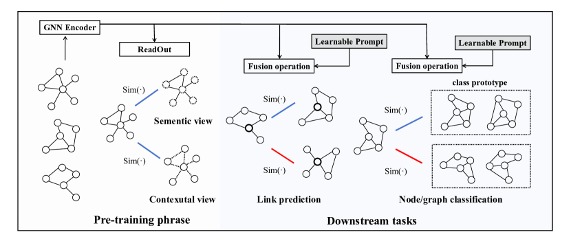
Figure 1. The overall framework of PGCL

4.1. Unified Framework

In the following, we present how the framework facilitates a unified perspective on pre-training and downstream tasks.

4.1.1. Graph instances under semantic and contextual view

Motivation of constructing graph instances. The success of prompts in NLP relies on the shared task template. However, graph-related tasks including node-level, edge-level and graph-level are far from similar. Generally, operations on graphs such as “modifying features” at node-level or “adding/deleting edges” at edge-level can both be considered as basic operations of graph-level. Compared with node-level and edge-level, graph-level tasks are more general and graph-level knowledge can be effectively transferred to other levels  (Sun et al., 2023). So we follow  (Sun et al., 2023; Liu et al., 2023a) and uniformly perform the node-level, edge-level tasks on graph-level through constructing graph instances. At node-level, we expand the target node $v$ on a graph $G=(V,E)$ into a subgraph $S_{v}=(V(S_{v}),E(S_{v}))$ of its local area, where its set of nodes and edges are respectively given by

(3) $$V(S_{v})=\{d(u,v)\leq\delta\mid u\in V\},$$

(4) $$E(S_{v})=\{(u,u^{\prime})\in E\mid u\in V(S_{v}),u^{\prime}\in V(S_{v})\},$$

where $d(u,v)$ gives the shortest distance between nodes $u$ and $v$ on $G$ and $\delta$ is a predetermined threshold. $S_{v}$ consists of nodes within $\delta$ hops from the node $v$, and the edges between those nodes. At graph-level, the maximum subgraph $S_{G}$ of a graph $G$ is the graph itself ( i.e., $S_{G}=G$), which naturally embodies the information of all nodes in $G$.
Semantic and contextual views. Since we use graph instances to represent both nodes and graphs, the (sub)graph where the graph instance resides preserves rich self-information and contextual information by neighboring node features and connections  (Huang and Zitnik, 2020; Liu et al., 2021; Zhang and Chen, 2018), which play distinct roles in various downstream tasks. Therefore, we establish two views, namely the semantic view and the contextual view, to capture the node feature information and the topological structure information of graph instances, respectively. The semantic view for a graph instance mainly focuses on the features of nodes. This view describes the nodes in the (sub)graph with their intrinsic properties. The contextual view for a graph instance primarily emphasizes the information derived from neighboring connections. This view characterizes nodes in the (sub)graph by considering their local neighborhoods, which is the main scope of most GNN encoders. By establishing and complementing semantic and contextual views, we aim to capture information from graphs in a more comprehensive manner.
Embedding of graph instances. To obtain the embedding $z_{x}$ of graph instance $x$, we follow the standard approach and employ a READOUT operation to aggregate the representations of nodes in the (sub)graph $S_{x}$ of $x$. Considering a $K$-layer GNN $f(\cdot)$ and node representation $h^{(k)}_{v}$ generated by it,

(5) $$z_{x}=f(S_{x})=\texttt{READOUT}({h^{(k)}_{v}:v\in V(S_{x}),k\in K}).$$

The choice of the aggregation scheme for READOUT is flexible, including sum, max and mean pooling and more advanced techniques  (Xu et al., 2019; Ying et al., 2018). We simply use sum pooling in our implementation.

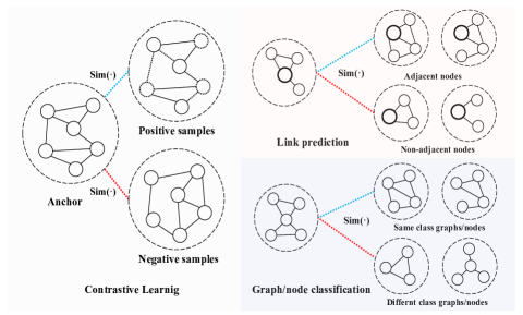
Figure 2. Illustration of the motivation.

4.1.2. Unified task template.

Motivation of adopting constrastive learning. Since we expand the target node into a graph instance, naturally we treat the target node’s label as this graph instance’s label. The same at edge-level, pair of nodes can be treated as a positive label if there is an edge connecting them, or a negative label if not. When we treat the edge’s label as this pair graph instances’ label, we can translate the edge-level task into the relationship learning between two graph instances. As can be seen in Fig. 2, link prediction is anchored on the similarity of representations for pairs of nodes. Intuitively, the representations of two adjacent nodes shall be more similar than those of non-adjacent nodes. For classification tasks, the graph/node representations of the same class shall exhibit higher similarity compared to those from different classes. It is worth noting that the core idea of contrastive learning is calculating the similarity between anchor and positive/negative sample with the goal of reducing the distance between the anchor and positive sample, while enlarging that between the anchor and negative sample. By similarity calculation in Fig. 2, we unify the graph contrastive learning as pretext with downstream tasks into a common task template.

Next, we will formally define the template for downstream tasks. Let $z_{x}$ be the representation vector of (sub)graph $S_{x}$ for graph instance $x$. How to fuse semantic and contextual information to obtain the representation of graph instance will be described in Section 4.3. Let $sim(\cdot,\cdot)$ be the cosine similarity function. Three downstream tasks (node classification, graph classification and link prediction) can be mapped to the similarity computation, which is formalized below.
Graph instance classification. Under our framework, node classification and graph classification are unified as graph instance classification. Consider a set of graph instances $\mathcal{G}$ with a set of classes $C$, and a set of labeled graph instances $\mathcal{D}=\{(G_{1},Y_{1}),(G_{2},Y_{2}),...\}$ where $G_{i}\in\mathcal{G}$ and $Y_{i}$ is the corresponding label of $G_{i}$. We follow the $k$-shot setting in  (Liu et al., 2023a), there are exactly $k$ pairs of $(G_{i},L_{i}=c)\in\mathcal{D}$ for each class $c\in C$. We define a class-prototype represented by $\tilde{z}_{c}$ for each class $c$. It is worth noting that the class-prototype is a “virtual” graph instance in the same latent space. The class-prototype representation can be obtained through representation learning (Sun et al., 2022). However, the representation learning of class-prototypes in few-shot settings poses challenges due to the limited annotated data. Therefore, we follow  (Liu et al., 2023a) and employ the mean representation of labeled graph instances for each class as class-prototypes:

(6) $$\widetilde{z_{c}}=\frac{1}{k}\sum\limits_{(G_{i},Y_{i})\in\mathcal{D},Y_{i}=c}z_{G_{i}}.$$

Given a graph instance $G_{j}$ not in the labeled set $\mathcal{D}$, its class label $Y_{j}$ shall be

(7) $$Y_{j}=\arg\max_{c\in C}sim(z_{G_{j}},\widetilde{z_{c}})$$

Intuitively, the graph instance shall belong to the class whose class-prototype is the most similar to itself.
Link prediction. Under our framework, link prediction are model as the similarity computation between pair graph instances. Given a graph $G=(V,E)$, a triplet of nodes $(v,a,b)$ such that $(a,b)\in E$ and $(v,b)\notin E$, we shall have

(8) $$sim(z_{v},z_{a})>sim(z_{v},z_{b})$$

It is worth noting that the link prediction task is based on the homophily assumption, i.e., the representation for $S_{v}$ of $v$ shall be more similar to that of a node adjacent to $v$ than that of another non-adjacent node.

In summary, we reformulated the pretext and downstream tasks on graphs into a common task template: the similarity learning among graph instances, which lays the foundation of our pre-training and prompting strategies as we will introduce in the following subsection.

4.2. Multi-View Pre-Training

In this section, we will introduce our multi-view pre-training strategy, which captures relevant information on graphs through semantic and contextual contrasts.
Semantic View. Semantic-level contrast aims to encourage the learned representations of graph instances with similar features to be consistent. Given a graph instance $x$ and its (sub)graph $S_{x}=(V,E)$, we employ a perturbation $\mathbf{\tau_{\alpha}}$ on the initial feature matrix $\mathbf{X}$ to generate a new feature matrix as the positive sample:

(9) $$\widetilde{\mathbf{X}}\sim\mathbf{\tau_{\alpha}}(\mathbf{X}),$$

where $\widetilde{\mathbf{X}}$ is the augmented feature matrix. We apply perturbations by altering only the features of nodes while keeping the graph structure unchanged. Specifically, we randomly mask the initial node features in different dimensionality with a probability. To independently encode the features without taking into account the structure information, we construct a unit matrix $\mathbf{I}\in\mathbb{R}^{|V|\times|V|}$ as the adjacency matrix and feed it into GNN $f(\cdot)$ along with features. The semantic representation obtained is denoted by $z^{s}$ and corresponding augmentation are denoted by $\widetilde{z^{s}}$:

(10) $$z^{s}=f_{\Theta}\left(\mathbf{X},\mathbf{I}\right),\widetilde{z^{s}}=f_{\Theta}\left(\widetilde{\mathbf{X}},\mathbf{I}\right),$$

where $\Theta$ denotes the parameters of GNN encoder. Then, a non-linear projection $g(\cdot)$ is used to map the representations to the latent space where the contrastive loss is applied, as advocated in (Chen et al., 2020). Specially, a two-layer perceptron (MLP) is applied to obtain $\mathbf{z}^{s}$ and $\widetilde{\mathbf{z}^{s}}$:

(11) $$\mathbf{z}^{s}=g(z^{s}),\widetilde{\mathbf{z}^{s}}=g(\widetilde{z^{s}}).$$

We construct the semantic-level contrastive loss based on the normalized temperature-scaled cross entropy loss (NT-Xent) (Chen et al., 2020). During pre-training phrase, we randomly select $N$ graph instances from the whole dataset as a mini-batch. For each graph instance $G_{i}$ in the mini-batch, we construct positive pairs $\left(\mathbf{z}_{G_{i}}^{s},\widetilde{\mathbf{z}_{G_{i}}^{s}}\right)$, negative pairs are not explicitly sampled but generated from the other graphs and their corresponding augmentations within the same minibatch. For convenience of expression, the semantic contrastive loss is formulated as:

(12) $$\mathcal{L}_{s}=-\frac{1}{N}\sum\limits_{i=1}^{N}\log\frac{exp(sim\left(\mathbf{z}_{G_{i}}^{s},\widetilde{\mathbf{z}_{G_{i}}^{s}}\right)/\tau)}{\sum^{N}_{j=1}exp(sim\left(\mathbf{z}_{G_{i}}^{s},\widetilde{\mathbf{z}_{G_{j}}^{s}}\right)/\tau)},$$

where $\tau$ denotes the temperature parameter to control the shape of the output distribution.
Contextual View. Context-level contrast aims to encourage graph instances with similar topology to be consistent. When constructing positive samples under the contextual view, it should be ensured that the semantic information of graph instances remains unchanged. Therefore, we only introduce a perturbation $\mathbf{\tau_{\beta}}$ on the adjacent matrix $\mathbf{A}$ while preserving the semantic information:

(13) $$\widetilde{\mathbf{A}}\sim\mathbf{\tau_{\beta}}\left(\mathbf{A}\right).$$

Specifically, we randomly drop some edges in the graph with a probability, which is equivalent to removing a small portion of nodes to alter the contextual information. To capture the contextual information of graph instance, we use feature matrix and adjacency matrix as the input of GNN $f(\cdot)$. The contextual representation obtained is denoted by $z^{c}$ and the corresponding augmentation are denoted by $\widetilde{z^{c}}$,

(14) $$z^{c}=f_{\Theta}\left(\mathbf{X},\mathbf{A}\right),\widetilde{z^{c}}=f_{\Theta}\left(\mathbf{X},\widetilde{\mathbf{A}}\right).$$

Similar as the contrastive loss under the semantic view, we construct the contextual contrastive loss after the non- linear projection $g(\cdot)$:

(15) $$\mathcal{L}_{c}=-\frac{1}{N}\sum\limits_{i=1}^{N}\log\frac{exp(sim\left(\mathbf{z}_{G_{i}}^{c},\widetilde{\mathbf{z}_{G_{i}}^{c}}\right)/\tau)}{\sum^{N}_{j=1}exp(sim\left(\mathbf{z}_{G_{i}}^{c},\widetilde{\mathbf{z}_{G_{j}}^{c}}\right)/\tau)}.$$

Note that we share the same GNN encoder between two views and the loss is parameterized by $\Theta$. To sum up, the pre-training loss $\mathcal{L}_{pre}$ can be defined as:

(16) $$\mathcal{L}_{pre}=\mathcal{L}_{s}+\lambda\mathcal{L}_{c},$$

where $\lambda$ are weight factors for adjusting the importance of two views. After pre-training, we freeze the model and then perform prompting on the outputs of model.

4.3. Prompt Design for Downstream Tasks

Aligning the pretext with downstream tasks can enable more effective knowledge transfer. We next show how to unify pre-training and downstream prompt-tuning.
Representation fusion and prompt design. From the macroscopic perspective, node features and graph topology are both essential components of a graph. To further enhance representation learning on graphs, we consider that the contextual information and the semantic information complement each other. We thus fuse them into a holistic representation that can adapt to different tasks. Here we simply use the CONCAT operation in our implementation. Formally, for each graph instance $x$, we fuse its semantic representation $z^{s}_{x}$ and contextual representation $z^{c}_{x}$ to obtain $x$’s representation $z_{x}=\texttt{CONCAT}(z^{s}_{x},z^{c}_{x})$. In this way, the similarity between two graph instances can be captured by their similarity in both semantic and contextual information. This also aligns with the pre-training objectives.

From the microscopic perspective, semantic view and contextual view play different roles in various tasks. For example, node classification (especially on heterophilous graphs) generally pays more attention to node features, while link prediction and graph classification focus on the structure information. Therefore, we should design prompts to extract the most relevant knowledge from representations of the two views. A naive way is to directly apply a linear transformation $\mathbf{P}$ as learnable prompt, which can be formulated as:

(17) $$z^{p}_{x}=\mathbf{P}\cdot\texttt{CONCAT}(z_{x}^{s},z_{x}^{c}),$$

where $z^{p}_{x}$ is the prompted representation for graph instance $x$. The linear transformation $\mathbf{P}$ can be regarded as a reweighting between semantic and contextual view to adjust the representation for downstream tasks.

Further, we can also introduce a prompt vector $\mathbf{p}^{s}$ for semantic view and $\mathbf{p}^{c}$ for contextual view, respectively. After that, for each view, we perform element-wise reweighting to extract more fine-grained irrelevant information and derive prompted semantic representation $z^{ps}_{x}$ and contextual representation $z^{pc}_{x}$:

(18) $$z^{ps}_{x}=z^{s}_{x}\odot\mathbf{p}^{s},z^{pc}_{x}=z^{c}_{x}\odot\mathbf{p}^{c},$$

where $\odot$ denotes the element-wise multiplication. Considering that the importance of these two views could vary in different tasks, we further employ a hyper-parameter $\alpha$ to control their weights and overload $z^{p}_{x}$ as:

(19) $$z^{p}_{x}=\texttt{CONCAT}(z^{ps}_{x},\alpha z^{pc}_{x}).$$

Note that $\alpha$ can be learned by using the attention mechanism. To align it with the pre-training objective, we set $\alpha=\lambda$ for simplicity in our implementation, where $\lambda$ is used in Equation 16 as a balance coefficient for the two views.

Prompt tuning. To optimize the learnable prompt parameters, we next formulate the loss functions in prompt tuning.

For node/graph classification, given a labeled training set $\mathcal{T}=\{(G_{1},Y_{1}),(G_{2},Y_{2}),\dots\}$ with a set of classes $C$, where $G_{i}$ is a labeled graph instance (e.g., a node or a graph) and $Y_{i}$ is the class label of $G_{i}$, the loss function for prompt tuning is then defined as:

(20) $$\mathcal{L}_{prompt}=-\sum\limits_{(G_{i},Y_{i})\in\mathcal{T}_{t}}\log\frac{exp(sim\left(z^{p}_{G_{i}},\widetilde{z^{p}_{Y_{i}}}\right)/\tau)}{\sum_{c\in Y}exp(sim\left(z^{p}_{G_{i}},\widetilde{z^{p}_{c}}\right)/\tau)},$$

where $\widetilde{z^{p}_{c}}$ denotes the prompted representation of prototype for class $c\in C$. For link prediction, given a node $v$ on graph $G$, we randomly sample one positive node $a$ from $v$’s adjacent neighbors, and one negative node $b$ that does not directly link to $v$, forming a triplet $(v,a,b)$. Our objective is to increase the similarity between graph instance $S_{v}$ and $S_{a}$, while decreasing that between $S_{v}$ and $S_{b}$. We sample a number of triplets from the graph to construct a training set $\mathcal{T}$. Then our objective is given as:

(21) $$\mathcal{L}_{prompt}=-\sum\limits_{(v,a,b)\in\mathcal{T}}\log\frac{exp(sim\left(z^{p}_{v},z^{p}_{a}\right)/\tau)}{\sum_{u\in\{x,y\}}exp(sim\left(z^{p}_{v},z^{p}_{u}\right)/\tau)}.$$

Note that, unlike fine-tuning, prompt tuning freezes parameters in the pre-training stage, while updating only a few parameters, e.g., $\mathbf{P}$ and $\mathbf{p}^{s},\mathbf{p}^{c}$ in our cases. This significantly decreases the difficulty in model training. More analysis about model complexity are presented in Appendix  6.

5. EXPERIMENTS

In this section, we perform experiments on benchmark datasets to evaluate the proposed PGCL.

5.1. Experimental Settings

Datasets. We employ 12 datasets in total, which can be divided into three groups. The first group is homophilous graphs, which include Cora, Citeseer, PubMed and DBLP (Sen et al., 2008; Bojchevski and Günnemann, 2017). These datasets are citation networks that are widely used for node classification and link predicion. In these datasets, nodes represent publications and edges are citations between them. Further, node features are the bag-of-words representations of keywords contained in the publications. The second group is heterophilous graphs. We adopt four public datasets from: Chameleon, Cornell, Texas, Wisconsin  (Pei et al., 2020). Specifically, these datasets are web networks, where nodes are web pages and edges are hyperlinks. The last group is graph classification dataset including PROTEINS, COX2, ENZYMES, BZR  (Borgwardt et al., 2005; Rossi and Ahmed, 2015; Wang et al., 2022). These datasets are a collection of molecular structure graphs.

Baselines. To evaluate the effectiveness of PGCL, we mainly compare it with the state-of-the-art approaches from three main categories (1) End-to-end GNN methods: GCN (Kipf and Welling, 2016a), GraphSAGE (Hamilton et al., 2017), GAT (Veličković et al., 2017), GIN (Xu et al., 2019) and H₂GCN (Zhu et al., 2020b). These methods directly train a GNN model on a specific task and work in an end-to-end manner. (2) Graph pre-training methods: GAE (VGAE)  (Kipf and Welling, 2016b), DGI (Veličković et al., 2018), InfoGraph (Sun et al., 2019), GRACE (Zhu et al., 2020a), MVGRL (Hassani and Khasahmadi, 2020) and GraphCL (You et al., 2020). These methods pre-train a GNN model in a self-supervised way work and fine-tune for the downstream task. (3) Graph prompt methods: GPPT  (Sun et al., 2022) and GraphPrompt  (Liu et al., 2023a). These methods utilize the link prediction task for pre-training, and reformulate downstream tasks into the common complate. Note that meta-learning methods cannot be compared in our setting, as they require labeled data in their base classes for the meta-training phase.

Setup. To evaluate the goal of PGCL  in better utilization of the capabilities of pre-trained model and generalizability of different tasks. We mainly consider three typical types of downstream tasks, i.e., node classification and graph classification in few-shot settings and link prediction. For node classification and graph classification, we follow GraphPrompt  (Liu et al., 2023a) and construct a series of $k$-shot classification tasks. The details of task construction will be elaborated later when reporting the results. For task evaluation, as the $k$-shot tasks are balanced classification, we employ accuracy as the evaluation metric. For all the baselines, based on the authors’ code and default settings, we further tune their hyper-parameters to optimize their performance.

Table 1. Node classification accuracy ($\%$) on homophilous graphs. We highlight the best score for each dataset in bold.

Method	Cora	Citeseer	PubMed	DBLP
GCN	43.04±8.06	33.83±9.53	54.38±7.59	42.93±10.85
GAT	45.33±7.01	36.72±8.52	55.74±9.12	38.63±9.83
GraphSAGE	43.27±8.05	32.68±10.23	54.32±10.11	39.91±12.68
GAE	42.51±6.53	40.68±9.23	51.72±8.92	39.73±12.05
DGI	49.41±7.72	43.19±8.73	50.30±7.89	42.38±9.57
MVGRL	56.02±7.86	46.25±8.98	54.29±8.83	45.14±10.71
GRACE	55.56±8.76	46.64±5.98	54.16±9.59	47.78±11.90
GPPT	51.63±8.76	42.89±7.93	50.98±9.12	39.48±12.08
GraphPrompt	55.32±9.56	44.19±9.73	53.49±8.68	43.32±10.87
PGCL	57.51±8.09	48.12±7.23	59.94±8.16	49.07±7.31

Table 2. Node classification accuracy ($\%$) on heterophilous graphs. For each dataset, we highlight the best result in bold.

Method	Chameleon	Cornell	Texas	Wisconsin
GCN	26.84±7.52	23.93±9.33	19.48±11.12	19.84±13.67
GAT	25.75±5.46	23.77±10.25	20.40±12.07	18.27±10.19
MLP	22.67±2.88	29.61±11.34	33.74±8.82	36.54±10.72
H2GCN	26.95±3.73	28.38±12.52	34.37±15.82	35.21±15.35
GAE	22.80±3.63	21.44±8.97	26.89±16.91	17.71±8.79
DGI	25.42±4.82	24.35±9.74	21.21±12.71	24.64±11.89
MVGRL	26.45±4.01	26.23±9.62	24.55±11.49	25.82±13.35
GRACE	24.68±3.79	19.51±8.07	18.58±9.36	19.95±9.94
GPPT	25.05±3.68	27.57±9.13	22.96±12.89	30.44±10.77
GraphPrompt	25.62±4.66	28.67±7.24	23.13±11.89	28.54±7.64
PGCL	30.45±3.14	39.52±8.71	40.17±7.88	47.48±10.24

5.2. Performance Comparison

We conduct various types of downstream task, namely, few-shot node classification on homophilous and heterophilous graphs, few-shot graph classification, and link prediction and compare the performance of PGCL  with other methods.

Few-shot on homophilous graphs. We conduct this node classification on homophilous graphs on four datasets, i.e., Cora, Citeseer, PubMed and DBLP. Following the $k$-shot setup  (Liu et al., 2023a), we generate a series of few-shot tasks for model training and validation. In particular, we randomly generate ten 1-shot node classification tasks (i.e., we randomly sample 1 node per class) for training and validation, respectively. Each training task is paired with a validation task, and the remaining nodes not sampled by the pair of training and validation tasks will be used for testing. Table  1 illustrates the results of few-shot node classification on homophilous graphs. We have the following observations:
(1) End-to-end GNN models achieve poor performance in most cases, demonstrating that they heavily depend on task-specific labeled data as supervision.
(2) Compared to end-to-end GNN models, pre-traing GNN models achieve even worse performance on PubMed. This implies that they have not effectively transferred knowledge to downstream tasks.
(3) PGCL  outperforms all the baselines across all datasets, demonstrating that the unified framework can fully leverage the capabilities of pre-trained models by aligning the objectives of pre-training and downstream tasks.
Few-shot on heterophilous graphs. We conduct this node classification on heterophilous graphs on four datasets, i.e., Chameleon, Cornell, Texas, Wisconsin. We following the $k$-shot setup of experiments on homophilous graphs. Note that we additionally consider MLP as our baseline in our experiments. Table 2 shows the results of few-shot node classification on heterophilous graphs. We have the following observations:
(1) PGCL  consistently leads to the best results on all the datasets and shows superiority over H₂GCN, which is specially designed for graphs with heterophily.
(2) GAE, GPPT and GraphPrompt achieve poor performance on heterophilic datasets. This implies that link prediction as pretext overemphasizes the structure information, thereby neglecting the important semantic information on graphs.
(3) MLP achieves good results on Cornell, Texas and Wisconsin, indicating that node features only can play a vital role. Basic GCN performs relatively well on Chameleon, suggesting that contextual information also counts too. Therefore, capturing information on graphs through semantic and contextual views in PGCL  provides a more comprehensive approach.
Few-shot on graph classification. We conduct this graph classification on four datasets, i.e., PROTEINS, ENZYMES, COX2, BZR. For each dataset, we randomly generate 100 5-shot classification tasks for training and validation, following a similar process for node classification tasks. We illustrate the results of few-shot graph classification in Table  3, and have the following observations:
(1) GraphPrompt and PGCL  outperform other baselines, once again demonstrating that the effectiveness of the prompt design and unified framework for pre-training and downstream tasks.
(2) Note that we use the raw features in these datasets to initialize input feature vectors, so PGCL  can simultaneously captures information from both features and graph structure. The superior results on graph classification demonstrate that the fusion operation of PGCL  provides more inter-class information in few-shot setting.
Link prediction. We conduct this link prediction on three datasets, i.e., Cora, Citeseer and PubMed. We follow previous studies  (Kipf and Welling, 2016b) to construct the train/valid/test edge sets. To be specific, we randomly split all edges into three sets, i.e., the training set (85%), the validation set (5%), and the test set (10%), and evaluate the performance based on AUC and AP scores. We compare our PGCL  with two generation-based methods: GAE and VGAE, and two contrastive methods: GRACE and MVGRL. Table  4 list the results and note that PGCL_np is our method without prompt tuning. We have the following observation:
(1) Generative baselines perform generally better than contrastive methods and PGCL_np, which is consistent with common belief.
(2) PGCL  leads to a much larger performance gap compared with MVP_np and performs generative baselines on Cora and Citeseer and achieves comparable results on PubMed, indicating that the prompt design effectively tune output of pre-trained model to adapt to downstream task.

Table 3. Graph classification accuracy ($\%$). For each dataset, we highlight the best result in bold.

Method	PROTEINS	ENZYMES	COX2	BZR
GCN	54.87±11.20	20.37±5.24	51.37±11.06	56.16±11.07
GAT	48.78±18.46	15.90±4.13	51.20±27.93	53.19±20.61
GraphSAGE	52.99±10.57	18.32±6.22	52.87±11.46	57.23±10.95
GIN	58.17±8.58	20.34±5.01	51.89±8.71	57.45±10.54
InfoGraph	54.12±8.20	20.90±3.32	54.04±9.45	57.57±9.93
GraphCL	56.38±7.24	28.11±4.00	55.40±12.04	59.22±7.42
GraphPrompt	64.42±4.37	31.45±4.32	59.21±6.82	61.63±7.68
PGCL	67.16±7.08	26.27±3.74	63.99±12.36	65.13±11.49

Table 4. Link prediction results. We highlight the best score on each dataset in bold.

Metric	Method	Cora	Citeseer	Pubmed
AUC	GAE	91.09±0.01	90.52±0.05	96.40±0.02
	VGAE	91.40±0.01	90.83±0.02	94.40±0.01
	MVGRL	88.21±0.50	89.95±0.40	91.43±0.59
	GRACE	87.29±0.37	88.64±0.96	94.39±0.82
	PGCL_np	84.56±0.33	75.13±0.74	88.25±0.91
	PGCL	92.70±0.15	94.53±0.30	94.86±0.25
AP	GAE	92.38±0.01	90.52±0.03	96.40±0.01
	VGAE	92.60±0.01	92.21±0.02	94.70±0.02
	MVGRL	89.61±0.70	89.37±0.35	94.66±0.45
	GRACE	85.73±0.43	89.95±0.40	93.83±1.03
	PGCL_np	85.62±0.78	77.38±0.64	89.67±0.46
	PGCL	92.81±0.40	94.62±0.21	94.74±0.40

6. Model Analysis

Time complexity. We analyze the time complexity of main components in our model. Assume an input graph has $n$ nodes and $m$ edges, let the GNN encoder contain $l$ layers. During the pre-training phrase, the time complexities of GNN encoder is $O(dml+nd^{\prime}dl)$, where $d$ is the dimensionality of initial features, $d^{\prime}$ is the dimensionality of final representations. Let $q$ be the number of selected negative samples in a batch, the complexity of contrastive loss is $O(nqd^{\prime})$. During the prompt tuning phrase, the time complexity for $k$-shot classification task with $c$ classes is $O(kc^{2}d^{\prime})$, and the time complexity for link prediction is $O(nd^{\prime})$. During the inference phrase, the time complexity for classification task is $O(cd^{\prime})$, and the time complexity for link prediction is $O(d^{\prime})$.
Parameter efficiency. We also compare the number of parameters that needs to be updated in a downstream classification task with a few representative models. As can be seen in Table  5, GCN works in an end-to-end manner, it is obvious that it involves the largest number of parameters for updating. GRACE and MVGRL employ a linear classifier for node classification, so the parameters in the classifier need to be updated in the downstream task. For our proposed PGCL, it not only outperforms the baselines GCN, GRACE and MVGRL as we have seen earlier, but also requires the least parameters, demonstrating the superiority of graph prompting.

Table 5. Study of parameter efficiency on node classification.

Method	Cora	Citeseer	PubMed	DBLP
GCN	18,430	474,752	64,384	210,304
GRACE	896	1,536	768	1,024
MVGRL	3,584	3,072	1,536	2,048
PGCL	256	256	256	256

7. CONCLUSIONS

In this paper, we proposed a multi-view pre-train and unified down-stream tasks prompting method PGCL. In particular, to narrow the gap between pre-training and downstream objectives on graph, we reformulated pre-training pretexts and downstream tasks on graphs into a common template. In the pre-training phase, we proposed a multi-view contrastive learning method to capture the semantic and contextual structure information on graphs. In the prompt tuning stage, we introduced a learnable prompt strategy to transfer the pre-trained knowledge to different downstream tasks. Finally, we extensively evaluated the performance of our method on 12 public datasets. Our experimental results demonstrate the effectiveness of our framework.

References

- (1)
- Bo et al. (2021) Deyu Bo, Xiao Wang, Chuan Shi, and Huawei Shen. 2021. Beyond low-frequency information in graph convolutional networks. In Proceedings of the AAAI Conference on Artificial Intelligence, Vol. 35. 3950–3957.
- Bojchevski and Günnemann (2017) Aleksandar Bojchevski and Stephan Günnemann. 2017. Deep gaussian embedding of graphs: Unsupervised inductive learning via ranking. arXiv preprint arXiv:1707.03815 (2017).
- Borgwardt et al. (2005) Karsten M Borgwardt, Cheng Soon Ong, Stefan Schönauer, SVN Vishwanathan, Alex J Smola, and Hans-Peter Kriegel. 2005. Protein function prediction via graph kernels. Bioinformatics 21, suppl_1 (2005), i47–i56.
- Brown et al. (2020) Tom Brown, Benjamin Mann, Nick Ryder, Melanie Subbiah, Jared D Kaplan, Prafulla Dhariwal, Arvind Neelakantan, Pranav Shyam, Girish Sastry, Amanda Askell, et al. 2020. Language models are few-shot learners. Advances in neural information processing systems 33 (2020), 1877–1901.
- Cai et al. (2018) Hongyun Cai, Vincent W Zheng, and Kevin Chen-Chuan Chang. 2018. A comprehensive survey of graph embedding: Problems, techniques, and applications. IEEE transactions on knowledge and data engineering 30, 9 (2018), 1616–1637.
- Chen et al. (2020) Ting Chen, Simon Kornblith, Mohammad Norouzi, and Geoffrey Hinton. 2020. A simple framework for contrastive learning of visual representations. In International conference on machine learning. PMLR, 1597–1607.
- Duvenaud et al. (2015) David K Duvenaud, Dougal Maclaurin, Jorge Iparraguirre, Rafael Bombarell, Timothy Hirzel, Alán Aspuru-Guzik, and Ryan P Adams. 2015. Convolutional networks on graphs for learning molecular fingerprints. Advances in neural information processing systems 28 (2015).
- Gao et al. (2020) Tianyu Gao, Adam Fisch, and Danqi Chen. 2020. Making pre-trained language models better few-shot learners. arXiv preprint arXiv:2012.15723 (2020).
- Gilmer et al. (2017) Justin Gilmer, Samuel S Schoenholz, Patrick F Riley, Oriol Vinyals, and George E Dahl. 2017. Neural message passing for quantum chemistry. In International conference on machine learning. PMLR, 1263–1272.
- Gu et al. (2021) Yuxian Gu, Xu Han, Zhiyuan Liu, and Minlie Huang. 2021. Ppt: Pre-trained prompt tuning for few-shot learning. arXiv preprint arXiv:2109.04332 (2021).
- Hamilton et al. (2017) Will Hamilton, Zhitao Ying, and Jure Leskovec. 2017. Inductive representation learning on large graphs. Advances in neural information processing systems 30 (2017).
- Hassani and Khasahmadi (2020) Kaveh Hassani and Amir Hosein Khasahmadi. 2020. Contrastive multi-view representation learning on graphs. In International conference on machine learning. PMLR, 4116–4126.
- Hou et al. (2022) Zhenyu Hou, Xiao Liu, Yukuo Cen, Yuxiao Dong, Hongxia Yang, Chunjie Wang, and Jie Tang. 2022. Graphmae: Self-supervised masked graph autoencoders. In Proceedings of the 28th ACM SIGKDD Conference on Knowledge Discovery and Data Mining. 594–604.
- Hu et al. (2019) Weihua Hu, Bowen Liu, Joseph Gomes, Marinka Zitnik, Percy Liang, Vijay Pande, and Jure Leskovec. 2019. Strategies for pre-training graph neural networks. arXiv preprint arXiv:1905.12265 (2019).
- Hu et al. (2020) Ziniu Hu, Yuxiao Dong, Kuansan Wang, Kai-Wei Chang, and Yizhou Sun. 2020. Gpt-gnn: Generative pre-training of graph neural networks. In Proceedings of the 26th ACM SIGKDD International Conference on Knowledge Discovery & Data Mining. 1857–1867.
- Huang and Zitnik (2020) Kexin Huang and Marinka Zitnik. 2020. Graph meta learning via local subgraphs. Advances in neural information processing systems 33 (2020), 5862–5874.
- Jin et al. (2020) Wei Jin, Tyler Derr, Haochen Liu, Yiqi Wang, Suhang Wang, Zitao Liu, and Jiliang Tang. 2020. Self-supervised learning on graphs: Deep insights and new direction. arXiv preprint arXiv:2006.10141 (2020).
- Kipf and Welling (2016a) Thomas N Kipf and Max Welling. 2016a. Semi-supervised classification with graph convolutional networks. arXiv preprint arXiv:1609.02907 (2016).
- Kipf and Welling (2016b) Thomas N Kipf and Max Welling. 2016b. Variational graph auto-encoders. arXiv preprint arXiv:1611.07308 (2016).
- Lester et al. (2021) Brian Lester, Rami Al-Rfou, and Noah Constant. 2021. The power of scale for parameter-efficient prompt tuning. arXiv preprint arXiv:2104.08691 (2021).
- Li et al. (2023) Xiang Li, Tiandi Ye, Caihua Shan, Dongsheng Li, and Ming Gao. 2023. SeeGera: Self-supervised Semi-implicit Graph Variational Auto-encoders with Masking. In Proceedings of the ACM Web Conference 2023. 143–153.
- Li et al. (2022) Xiang Li, Renyu Zhu, Yao Cheng, Caihua Shan, Siqiang Luo, Dongsheng Li, and Weining Qian. 2022. Finding global homophily in graph neural networks when meeting heterophily. In International Conference on Machine Learning. PMLR, 13242–13256.
- Li and Liang (2021) Xiang Lisa Li and Percy Liang. 2021. Prefix-tuning: Optimizing continuous prompts for generation. arXiv preprint arXiv:2101.00190 (2021).
- Liu et al. (2022) Xiao Liu, Kaixuan Ji, Yicheng Fu, Weng Tam, Zhengxiao Du, Zhilin Yang, and Jie Tang. 2022. P-tuning: Prompt tuning can be comparable to fine-tuning across scales and tasks. In Proceedings of the 60th Annual Meeting of the Association for Computational Linguistics (Volume 2: Short Papers). 61–68.
- Liu et al. (2023b) Yixin Liu, Yizhen Zheng, Daokun Zhang, Vincent CS Lee, and Shirui Pan. 2023b. Beyond smoothing: Unsupervised graph representation learning with edge heterophily discriminating. In Proceedings of the AAAI conference on artificial intelligence, Vol. 37. 4516–4524.
- Liu et al. (2021) Zemin Liu, Yuan Fang, Chenghao Liu, and Steven CH Hoi. 2021. Node-wise localization of graph neural networks. arXiv preprint arXiv:2110.14322 (2021).
- Liu et al. (2023a) Zemin Liu, Xingtong Yu, Yuan Fang, and Xinming Zhang. 2023a. Graphprompt: Unifying pre-training and downstream tasks for graph neural networks. In Proceedings of the ACM Web Conference 2023. 417–428.
- Lu et al. (2021) Yuanfu Lu, Xunqiang Jiang, Yuan Fang, and Chuan Shi. 2021. Learning to pre-train graph neural networks. In Proceedings of the AAAI conference on artificial intelligence, Vol. 35. 4276–4284.
- Pei et al. (2020) Hongbin Pei, Bingzhe Wei, Kevin Chen-Chuan Chang, Yu Lei, and Bo Yang. 2020. Geom-gcn: Geometric graph convolutional networks. arXiv preprint arXiv:2002.05287 (2020).
- Qiu et al. (2020) Jiezhong Qiu, Qibin Chen, Yuxiao Dong, Jing Zhang, Hongxia Yang, Ming Ding, Kuansan Wang, and Jie Tang. 2020. Gcc: Graph contrastive coding for graph neural network pre-training. In Proceedings of the 26th ACM SIGKDD international conference on knowledge discovery & data mining. 1150–1160.
- Rossi and Ahmed (2015) Ryan Rossi and Nesreen Ahmed. 2015. The network data repository with interactive graph analytics and visualization. In Proceedings of the AAAI conference on artificial intelligence, Vol. 29.
- Schick and Schütze (2020) Timo Schick and Hinrich Schütze. 2020. Exploiting cloze questions for few shot text classification and natural language inference. arXiv preprint arXiv:2001.07676 (2020).
- Sen et al. (2008) Prithviraj Sen, Galileo Namata, Mustafa Bilgic, Lise Getoor, Brian Galligher, and Tina Eliassi-Rad. 2008. Collective classification in network data. AI magazine 29, 3 (2008), 93–93.
- Shen et al. (2021) Zheyan Shen, Jiashuo Liu, Yue He, Xingxuan Zhang, Renzhe Xu, Han Yu, and Peng Cui. 2021. Towards out-of-distribution generalization: A survey. arXiv preprint arXiv:2108.13624 (2021).
- Sun et al. (2019) Fan-Yun Sun, Jordan Hoffmann, Vikas Verma, and Jian Tang. 2019. Infograph: Unsupervised and semi-supervised graph-level representation learning via mutual information maximization. arXiv preprint arXiv:1908.01000 (2019).
- Sun et al. (2022) Mingchen Sun, Kaixiong Zhou, Xin He, Ying Wang, and Xin Wang. 2022. Gppt: Graph pre-training and prompt tuning to generalize graph neural networks. In Proceedings of the 28th ACM SIGKDD Conference on Knowledge Discovery and Data Mining. 1717–1727.
- Sun et al. (2023) Xiangguo Sun, Hong Cheng, Jia Li, Bo Liu, and Jihong Guan. 2023. All in One: Multi-Task Prompting for Graph Neural Networks. (2023).
- Suresh et al. (2021) Susheel Suresh, Vinith Budde, Jennifer Neville, Pan Li, and Jianzhu Ma. 2021. Breaking the limit of graph neural networks by improving the assortativity of graphs with local mixing patterns. In Proceedings of the 27th ACM SIGKDD Conference on Knowledge Discovery & Data Mining. 1541–1551.
- Tang et al. (2022) Mingyue Tang, Carl Yang, and Pan Li. 2022. Graph auto-encoder via neighborhood wasserstein reconstruction. arXiv preprint arXiv:2202.09025 (2022).
- Veličković et al. (2017) Petar Veličković, Guillem Cucurull, Arantxa Casanova, Adriana Romero, Pietro Lio, and Yoshua Bengio. 2017. Graph attention networks. arXiv preprint arXiv:1710.10903 (2017).
- Veličković et al. (2018) Petar Veličković, William Fedus, William L Hamilton, Pietro Liò, Yoshua Bengio, and R Devon Hjelm. 2018. Deep graph infomax. arXiv preprint arXiv:1809.10341 (2018).
- Wang et al. (2021) Liyuan Wang, Mingtian Zhang, Zhongfan Jia, Qian Li, Chenglong Bao, Kaisheng Ma, Jun Zhu, and Yi Zhong. 2021. Afec: Active forgetting of negative transfer in continual learning. Advances in Neural Information Processing Systems 34 (2021), 22379–22391.
- Wang et al. (2022) Song Wang, Yushun Dong, Xiao Huang, Chen Chen, and Jundong Li. 2022. Faith: Few-shot graph classification with hierarchical task graphs. arXiv preprint arXiv:2205.02435 (2022).
- Xu et al. (2019) Keyulu Xu, Weihua Hu, Jure Leskovec, and Stefanie Jegelka. 2019. How Powerful are Graph Neural Networks?. In International Conference on Learning Representations. https://openreview.net/forum?id=ryGs6iA5Km
- Ying et al. (2018) Zhitao Ying, Jiaxuan You, Christopher Morris, Xiang Ren, Will Hamilton, and Jure Leskovec. 2018. Hierarchical graph representation learning with differentiable pooling. Advances in neural information processing systems 31 (2018).
- You et al. (2020) Yuning You, Tianlong Chen, Yongduo Sui, Ting Chen, Zhangyang Wang, and Yang Shen. 2020. Graph contrastive learning with augmentations. Advances in neural information processing systems 33 (2020), 5812–5823.
- Zhang and Chen (2018) Muhan Zhang and Yixin Chen. 2018. Link prediction based on graph neural networks. Advances in neural information processing systems 31 (2018).
- Zhong et al. (2021) Zexuan Zhong, Dan Friedman, and Danqi Chen. 2021. Factual probing is [mask]: Learning vs. learning to recall. arXiv preprint arXiv:2104.05240 (2021).
- Zhu et al. (2020b) Jiong Zhu, Yujun Yan, Lingxiao Zhao, Mark Heimann, Leman Akoglu, and Danai Koutra. 2020b. Beyond homophily in graph neural networks: Current limitations and effective designs. Advances in neural information processing systems 33 (2020), 7793–7804.
- Zhu et al. (2020a) Yanqiao Zhu, Yichen Xu, Feng Yu, Qiang Liu, Shu Wu, and Liang Wang. 2020a. Deep graph contrastive representation learning. arXiv preprint arXiv:2006.04131 (2020).